Embed Size (px)
Citation preview
International Journal of Forecasting ( ) –
Contents lists available at ScienceDirect
International Journal of Forecasting
journal homepage: www.elsevier.com/locate/ijforecast
Testing the value of probability forecasts forcalibrated combiningKajal Lahiri ∗, Huaming Peng, Yongchen ZhaoDepartment of Economics, University at Albany, SUNY, Albany, NY, 12222, USA
a r t i c l e i n f o
Keywords:SPF recession forecastsWelch-type testsAutocorrelation and skewness correctionsBeta-transfromed pool
a b s t r a c t
We combine the probability forecasts of a real GDP decline from the US Survey ofProfessional Forecasters, after trimming the forecasts that do not have ‘‘value’’, asmeasuredby the Kuiper Skill Score and in the sense of Merton (1981). For this purpose, we use asimple test to evaluate the probability forecasts. The proposed test does not require theprobabilities to be converted to binary forecasts before testing, and it accommodates serialcorrelation and skewness in the forecasts. We find that the number of forecasters makingvaluable forecasts decreases sharply as the horizon increases. The beta-transformedlinear pool combination scheme, based on the valuable individual forecasts, is shown tooutperform the simple average for all horizons on a number of performance measures,including calibration and sharpness. The test helps to identify the good forecasters ex ante,and therefore contributes to the accuracy of the combined forecasts.© 2014 International Institute of Forecasters. Published by Elsevier B.V. All rights reserved.
1. Introduction
Currently, more than forty-five years of quarterly ex-pert forecasts for a number of USmacroeconomic variablesare available in the US Survey of Professional Forecasters(SPF).1 In particular, the SPF probabilities of real GDP de-clines for the current quarter and the next four quartershave attracted special interest from economists and themass media alike. The New York Times columnist DavidLeonhardt (September 1, 2002) called the one-quarter-ahead GDP decline probability the ‘‘Anxious Index’’.Drawing on methodologies developed in statistics, theatmospheric sciences, and psychology, economists havestudied the quality and characteristics of these subjective
∗ Corresponding author.E-mail addresses: [email protected] (K. Lahiri), [email protected]
(H. Peng), [email protected] (Y. Zhao).1 The European Central Bank, the Banco de Mexico and the Reserve
Bank of India have also been collecting similar forecasts under the samename. Thus, any methodological improvement in the use of the US datawill be useful for a number of countries as well.
probabilities, and have reached a certain broad consensus.2First, a simple average of the individual probabilities seemsto encompass all of the information embedded in the in-dividual forecasts (Clements & Harvey, 2011); and second,these average forecast probabilities do not seem to haveany predictive power beyond the second quarter (Lahiri& Wang, 2013). Many researchers have noted the limita-tions of these average probabilities in forecasting economicdownturns. Stock andWatson (2003) point out that the SPFcould not foresee the 2001 recession: the signal camewitha lag in 2001:Q4, when the negative growth period had al-ready passed. Rudebusch and Williams (2009) show thatthe SPF participants do not seem to use the informationin the yield spread (i.e., the difference between long-termand short-term interest rates) in forecasting recessions, de-spite it having been well-known since at least the 1980s
2 See for instance Braun and Yaniv (1992), Clements (2008, 2009,2011), Clements and Harvey (2011), Engelberg, Manski, and Williams(2010), Galbraith and vanNorden (2011, 2012), Graham (1996), and Lahiriand Wang (2006, 2013).
http://dx.doi.org/10.1016/j.ijforecast.2014.03.0050169-2070/© 2014 International Institute of Forecasters. Published by Elsevier B.V. All rights reserved.
2 K. Lahiri et al. / International Journal of Forecasting ( ) –
that the yield spread is useful in forecasting real GDPgrowth and recessions. However, Lahiri, Monokroussos,and Zhao (2013) find that, when averaged over the rela-tively better forecasters, the combined SPF forecasts do in-corporate the information from the yield spread, as well asthat from amyriad of other economic indicators. Galbraithand van Norden (2012) use the pioneering ‘‘fan charts’’ ofthe Bank of England to calculate the probability that theannual rates of inflation and output growth will exceedgiven thresholds. They find a serious departure of these ag-gregate forecasts from perfect calibration and reasonablesharpness.
The main motivation of this paper comes from a recentfinding by Ranjan and Gneiting (2010) that the linearopinion pool is sub-optimal in terms of calibration andsharpness. Following their suggestion, we use the non-linearly recalibrated beta-transformed linear pool (BLP)to determine whether the performance of aggregatedSPF forecasts can be improved. As the fallout from therecent recession of 2007–2009 has painfully remindedus again, even a small improvement in our capability toforesee recessions is of enormous benefit to any modernsociety. Our second motivation is derived from the novelmethodological approach to forecast combination by Aiolfiand Timmermann (2006). Following their approach, anddue to the huge amount of missing data in the SPF, wefirst sort all of the forecasters into four clusters basedon their past performances. Then, we pool the forecastswithin each cluster, and follow this with an applicationof the BLP methodology to the cluster-level aggregates, inorder to obtain an improved combined forecast. However,before constructing the clusters, we trim the forecasterswhose forecasts are found to have no value in the senseof the Kuiper Skill Score (KSS), which is a sample analogof the concept of ‘‘value’’ in Merton (1981). Stekler (1994)initiated a very important line of research in this area offorecast evaluation, see also Schnader and Stekler (1990).For assessing the ‘‘value’’ of the forecasts, we proposeto use a Welch-type test3 that explicitly addresses thepotential issue of serial correlation and skewness.
The plan of the paper is as follows. In Section 2, wedescribe the nature and characteristics of the SPF proba-bility forecasts, which naturally leads on to the method-ological approach undertaken in this paper. In Section 3,we describe the test for zero forecast value and discuss itsrobustness to serial correlation and skewness. Section 4 re-ports our empirical results, including the test results, thebeta-transformed linear pool methodology, the combina-tion of the valuable forecasts, and a detailed evaluation ofthe combined forecasts in- and out-of-sample. Section 5concludes.
3 TheWelch-type t test is amodified Student’s t-test which is designedto test the equality of twomeanswith possibly unequal variances. That is,tυ =
µ1−µ2s21N1
+s22N2
, whereµi , s2i and Ni are the sample mean, sample variance
and sample size respectively for i = 1, 2, and the degrees of freedom υ is
given approximately by υ ≈
s21N1
+s22N2
2/
s41N21 (N1−1)
+s42
N22 (N2−1)
.
2. Probability forecasts in SPF
We use the probability forecasts of real GDP declinesfrom the US Survey of Professional Forecasters (SPF). TheSPF is the oldest quarterly survey of macroeconomic fore-casts in the United States.4 Since 1990Q2, the survey hasbeen being administered by the Federal Reserve Bank ofPhiladelphia. Survey respondents are asked to supply pointand density forecasts for a wide range of variables cover-ing output, prices, and employment situations. The surveyis usedwidely by researchers. Examples of recent work us-ing data from the survey include the studies by Capistranand Timmermann (2009), Clements (2011), and Lahiri andWang (2013). We examine the probability forecasts of realGDP declines for the current quarter (denoted h = 0)5 andthe following four quarters (h = 1, . . . , 4). The equally-weighted average of individual forecasts, i.e., the equally-weighted linear opinion pool (ELP), is used as a benchmarkwhen evaluating the performance of the combined fore-casts we construct. Our data spans the 174 quarters from1968Q4 to 2012Q1. A total of 32,379 forecasts are availablefrom 426 forecasters for 5 horizons.
Frequent data revisions and definitional changes affectreal GDP values after their initial release. In practice, suchchanges are rarely predictable before they are announced.The choice of actual values between an earlier data vintageand the latest vintage depends crucially on the objectivefunction of a forecasting client. We construct the binaryoutcome series (the actual values) yt using the firstvintage in the Real-Time Data Set for Macroeconomistsavailable from the Federal Reserve Bank of Philadelphia.6For a discussion of the real time data issues involvedin evaluating SPF forecasts, see Stark (2010). The sameapproach is taken by, among others, Clements and Harvey(2010). Our binary outcome series contains 24 quarters ofreal GDP declines, which is about 14% of the sample. Sincea real GDP decline is a relatively uncommon event, specialconsiderations are needed in forecast evaluation. Examplesof recent work focusing on evaluating probability forecastsinclude the studies by Galbraith and van Norden (2012)and Lahiri and Wang (2013).
The SPF contains a large amount of missing data,see Capistran and Timmermann (2009) and Lahiri, Peng,and Zhao (2012). In our case, more than 91% of the datais missing.7 To make the situation more complicated, af-ter the Federal Reserve Bank took over the survey, mostof the old forecasters stopped forecasting and many newforecasters joined the sample. As a result, for most of the
4 The survey was introduced in 1968 by the American StatisticalAssociation and the National Bureau of Economic Research. For moreinformation and background about the survey, see Croushore (1993). Thesurvey itself can be accessed from http://www.phil.frb.org/research-and-data/real-time-center/survey-of-professional-forecasters/.5 The ‘‘current quarter’’ refers to the quarter in which the survey is
conducted.6 A robustness check was conducted using the latest vintage, and our
main conclusions remained the same. Results from the robustness checkare available from the authors.7 A fully balanced panel with all forecasters who have ever partic-
ipated and all quarters would have 426 forecasters × 174 quarters ×
5 horizons = 370,620 forecasts; but we have only 32,379 forecasts.

K. Lahiri et al. / International Journal of Forecasting ( ) – 3
Table 1Descriptive statistics on individual QPS and skill scores. This table gives descriptive statistics on individual forecasters’ QPS and skill scores for thosesatisfying the participation requirement. (A naïve forecast of 14% is used to calculate skill score.)
Subsample Horizon Number of forecasters QPS Mean skill scoreMean Std. dev. Max Min
1969:I–1990:I
0 51 0.124 0.043 0.049 0.225 0.3831 48 0.170 0.040 0.084 0.255 0.1782 48 0.195 0.038 0.110 0.284 0.0743 49 0.225 0.046 0.136 0.315 −0.0374 47 0.255 0.058 0.159 0.369 −0.117
1990:II–2011:IV
0 47 0.067 0.041 0.015 0.278 0.3921 45 0.081 0.043 0.030 0.297 0.2832 44 0.101 0.049 0.041 0.263 0.1203 43 0.126 0.065 0.054 0.351 −0.0234 42 0.128 0.067 0.052 0.400 −0.074
old forecasters, no forecasts are available after 1990Q2, be-fore which there is obviously nothing available from thenewly joined forecasters. To address this issue, we split thesample at 1990Q2, thus creating two subsamples.8 Sub-sample 1 (the earlier subsample) has 275 forecasters. Sub-sample 2 has 158 forecasters. To further limit the amountof missing data, we impose a participation requirement. Asimple requirement asking formore than a certain numberof forecasts from a forecaster would not work in our case.This is because, for many forecasters who satisfy such arequirement, all of their forecasts would have come fromquarters without a real GDP decline. Therefore, we imposethe requirement separately on the quarters with andwith-out a real GDP decline: for each forecaster in subsample 1(2), we require at least 7 (3) forecasts from quarters with adecline in real GDP and at least 7 (3) forecasts from quar-ters with a growth in real GDP. This leaves us around 50forecasters for each horizon.9 Imposing this requirementdecreases the amount of missing data from 86% to 56% forsubsample 1 and from 78% to 55% for subsample 2.
Table 1 shows several descriptive statistics on individ-ual QPSs10 and skill scores for those satisfying the partici-pation requirement. As horizon increases, the mean valueof the individual QPS deteriorates from 0.12 for current-quarter forecasts to 0.26 for four-quarter-ahead forecastsin subsample 1, and from 0.07 to 0.13 in subsample 2. Thestandard deviation of the QPS scores increases slightly aswell: from 0.04 to around 0.06 as the forecast horizon in-creases in both subsamples. In general, the forecasting per-formance of these frequent forecasters seem to be betterin the later years (subsample 2) than in the earlier years.Across horizons, for both subsamples, a clear deteriora-tion in performance is observed at around the two-quarterhorizon.
8 Using the sample in its entirety does not alter our results qualitatively.9 We also carried out our analysis with this requirement increased to
10 (5) and decreased to 5 (2) for subsample 1 (2), and reached similarconclusions. Note that a requirement higher than 7 would filter out allforecasters joining the survey after the 1990s, since there have not beenmore than 7 quarters with a real GDP decline in the later period.10 The Brier’s Quadratic Probability Score (QPS) is a commonlyused measure of forecast accuracy, being a probability analog of themean squared error. See Lahiri and Wang (2013) for its definition,decomposition, and application in evaluating probability forecasts.
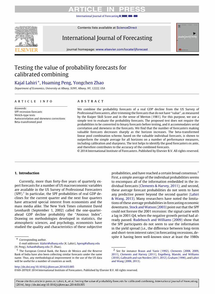
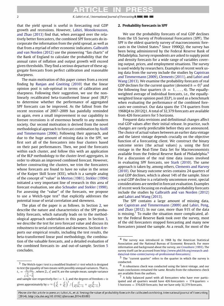
The Kuiper Skill Scores (KSS)11 for forecasters satisfyingthe participation requirement are shown in Fig. 1a for sub-sample 1 and in Fig. 1b for subsample 2. These individualKuiper scores are ranked and plotted on the vertical axisfor all five horizons, with the number of forecasters be-ing plotted on the horizontal axis. Each point in the graphrepresents one forecaster. Points joined by a curve rep-resent forecasters who are forecasting for the same hori-zon. For each horizon, forecasters are ranked based on theirKSS. The longer a curve, i.e., the more points connectedby a curve, the more forecasters there are for the horizonrepresented by the curve. Ideally, the curves for shorterhorizons should sit above the curves for longer horizons,representing a deterioration of KSS as the horizon in-creases. The steeper a curve is, the more rapidly KSS dete-riorates from the best forecaster to the worst forecaster fora given horizon. We see from the top plot in both Figs. 1aand 1b that the forecasts for the current quarter are signif-icantly better than those for the remaining quarters. Theperformance of these forecasts deteriorate greatly from thecurrent quarter to one quarter ahead for both subsamples,but only modestly from one to two quarters ahead for sub-sample 1. Little deterioration in KSSs is observed betweenthe three- and four-quarter-ahead forecasts. The best fore-casters for the two-, three-, and four-quarter-ahead hori-zons have almost the same performances. A zero or neg-ative KSS is first observed at the two-quarter horizon.Within each quarter, the KSSs of the best few forecastersand those of the worst few forecasters are widely differ-ent, while the KSSs for forecasters in the middle are rathersimilar.
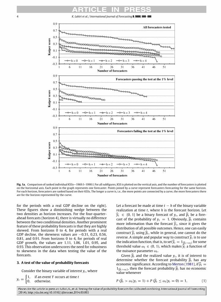
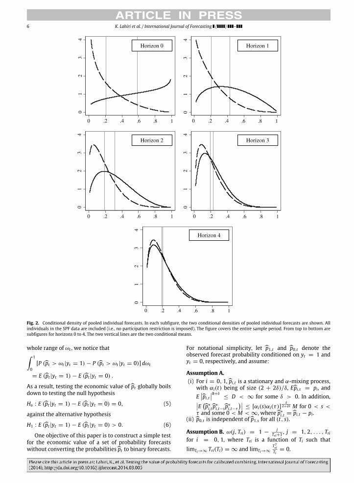
To further illustrate some common characteristics ofthese probability forecasts, we collect all of the individualforecasts horizon by horizon, conditioned on the outcome,and fit a beta distribution to them. We present these fitteddensities in Fig. 2, where two such conditional densitiesare plotted for each horizon, together with the associatedmean values (shown by vertical lines, with the mean value
11 The Kuiper (or Peirce) skill score is defined as KSS(ωt ) =Tt=1 I{pt>ωt ,yt=1}
I{yt=1}−
Tt=1 I{pt>ωt ,yt=0}
I{yt=0}for some threshold probability value
ωt > 0. Assume also that I{yt=1} , I{yt=0} , I{pt>ωt ,yt=1} , and I{pt>ωt ,yt=0}are stationary and ergodic over time; then, it can be shown that theprobability limit of KSS converges to P(pt > ωt |yt = 1)−P(pt > ωt |yt =
0), which is a function of ωt .
4 K. Lahiri et al. / International Journal of Forecasting ( ) –
Fig. 1a. Comparison of ranked individual KSSs—1969:I–1990:I. For all subfigures, KSS is plotted on the vertical axis, and the number of forecasters is plottedon the horizontal axis. Each point in the graph represents one forecaster. Points joined by a curve represent forecasters forecasting for the same horizon.For each horizon, forecasters are ranked based on their KSSs. The longer a curve is, i.e., themore points are connected by a curve, themore forecasters thereare for the horizon represented by the curve.
for the periods with a real GDP decline on the right).These figures show a diminishing wedge between thetwo densities as horizon increases. For the four-quarter-ahead forecasts (horizon 4), there is virtually no differencebetween the two conditional densities. Another prominentfeature of these probability forecasts is that they are highlyskewed. From horizons 0 to 4, for periods with a realGDP decline, the skewness values are −0.31, 0.23, 0.56,0.81, and 0.91. From horizons 0 to 4, for periods of realGDP growth, the values are 1.11, 1.06, 1.01, 0.95, and0.93. This observation underscores the need for robustnessto skewness in the data when testing the value of theforecasts.
3. A test of the value of probability forecasts
Consider the binary variable of interest yt , where
yt =
1, if an event Y occurs at time t0, otherwise.
Let a forecast be made at time t − h of the binary variablerealization at time t , where h is the forecast horizon. Letyt ∈ {0, 1} be a binary forecast of yt , andpt be a fore-cast of the probability of yt = 1. Obviously,pt containsmore information than the forecastyt , since it gives thedistribution of all possible outcomes. Hence, one can easilyconstructyt usingpt , while in general, one cannot do thereverse. A simple and popular way to constructyt is to usethe indication function, that is, to setyt = 1{pt>ωt } for somethreshold value ωt ∈ (0, 1), which makesyt a function ofthe nuisance parameter ωt .
Givenpt and the realized value yt , it is of interest todetermine whether the forecast probability pt has anyeconomic significance. According to Merton (1981), ifyt =
1{pt>ωt }, then the forecast probabilitypt has no economicvalue whenever
P (pt > ωt |yt = 1) + P (pt ≤ ωt |yt = 0) = 1, (1)
K. Lahiri et al. / International Journal of Forecasting ( ) – 5
Fig. 1b. Comparison of ranked individual KSSs—1990:II–2011:IV. For all subfigures, KSS is plotted on the vertical axis, and the number of forecasters isplotted on the horizontal axis. Each point in the graph represents one forecaster. Points joined by a curve represent forecasters forecasting for the samehorizon. For each horizon, forecasters are ranked based on their KSSs. The longer a curve is, i.e., the more points are connected by a curve, the moreforecasters there are for the horizon represented by the curve.
andpt is valuable if and only if
P (pt > ωt |yt = 1) + P (pt ≤ ωt |yt = 0) > 1. (2)
Merton (1981) argues that the larger the value ofthe sum P (pt > ωt |yt = 1) + P (pt ≤ ωt |yt = 0), themore valuable the forecasts pt .12 From the property ofdiscrete conditional probability, it can be seen that the twoconditions in Eqs. (1) and (2) are equivalent to
P (pt > ωt |yt = 1) − P (pt > ωt |yt = 0) = 0, (3)
and
P (pt > ωt |yt = 1) − P (pt > ωt |yt = 0) > 0, (4)
respectively. Note that P(pt > ωt |yt = 1) and P(pt >ωt |yt = 0) are the hit rate and the false alarm rate (or their
12 See Schnader and Stekler (1990) and Stekler (1994) for an earlyexplication of the concept and an application tomacroeconomic forecasts.
respective probability limits), becauseyt = 1 wheneverpt > ωt . Thus, the forecast probability pt has positiveeconomic value if and only if the (limit of the) Kuiper score,defined as the difference between the hit rate and the falsealarm rate, is positive. The application of the Kuiper scoreas an indication of the economic value of forecasts of binaryevents has also been justified by Granger and Pesaran(2000). Intuitively, in order for a forecast to be valuable inMerton’s sense, it is both necessary and sufficient that itshould outperform some random forecastswith an averageof zero Kuiper score.
However, the (limit of the) Kuiper score, as on theleft hand side of Eqs. (3) and (4), depends on the thresh-old probability ωt . The Kuiper score calculated using thethreshold ωt clearly has a ‘‘pointwise’’ property. Since thetest statistic, and statistical inference in general, vary withωt , it would only determine the economic value of fore-casts conditional on the specific ωt . To construct a hypoth-esis test of economic value that is globally valid for the
6 K. Lahiri et al. / International Journal of Forecasting ( ) –
01
23
4
01
23
40
12
34
01
23
4
01
23
4
.6 .8 1
0 .2 .4
0 .2 .4 .6 .8 10 .2 .4
.6 .8 10 .2 .4
.6 .8 10 .2 .4
.6 .8 1
Fig. 2. Conditional density of pooled individual forecasts. In each subfigure, the two conditional densities of pooled individual forecasts are shown. Allindividuals in the SPF data are included (i.e., no participation restriction is imposed). The figure covers the entire sample period. From top to bottom aresubfigures for horizons 0 to 4. The two vertical lines are the two conditional means.
whole range of ωt , we notice that 1
0[P (pt > ωt |yt = 1) − P (pt > ωt |yt = 0)] dωt
= E (pt |yt = 1) − E (pt |yt = 0) .
As a result, testing the economic value ofpt globally boilsdown to testing the null hypothesis
Ho : E (pt |yt = 1) − E (pt |yt = 0) = 0, (5)
against the alternative hypothesis
H1 : E (pt |yt = 1) − E (pt |yt = 0) > 0. (6)
One objective of this paper is to construct a simple testfor the economic value of a set of probability forecastswithout converting the probabilitiespt to binary forecasts.
For notational simplicity, let p1,t and p0,t denote theobserved forecast probability conditioned on yt = 1 andyt = 0, respectively, and assume:
Assumption A.(i) For i = 0, 1,pi,t is a stationary and α-mixing process,
with αi(t) being of size (2 + 2δ)/δ, Epi,t = pi, andEpi,t 8+δ
≤ D < ∞ for some δ > 0. In addition,E p∗
i,tp∗
i,t−sp∗
i,t−τ
≤ [αi(s)αi(τ )]δ
2+2δ M for 0 < s <τ and some 0 < M < ∞, wherep∗
i,t =pi,t − pi.(ii) p0,t is independent ofp1,s for all (t, s).Assumption B. ω(j, Tri) = 1 −
jTri+1 , j = 1, 2, . . . , Tri
for i = 0, 1, where Tri is a function of Ti such that
limTi→∞ Tri(Ti) = ∞ and limTi→∞
T7riTi
= 0.
K. Lahiri et al. / International Journal of Forecasting ( ) – 7
Assumption A allows for some weak dependence overtime in the probability forecast pi,t . The size of strongmixing, which controls the rate of dependence, along withthe moment condition restriction and the independencebetween the two processes, is important for derivingthe asymptotic normal distribution via the central limittheorem for dependent data. Assumption B, together withthe rate restriction on E
p∗
i,tp∗
i,t−sp∗
i,t−τ
, enables us to
obtain HAC estimators for both the long-run variance andskewness in the spirit of Newey and West (1987, 1994),and is fairly standard in the literature dealing with HACestimators. Taken together, Assumptions A and B specifythe dynamic properties of the two probability forecastprocesses and the conditions that allow us to carry out asimple one-sided test for the economic value ofpt .
A number of statistical tests for the economic valueof directional forecasts have been proposed in the liter-ature. Henriksson and Merton (1981) introduced a sta-tistical test of forecasting skill that is closely related toFisher’s exact tests for testing the null of independence be-tween two binary variables, cf. Stekler (1994). Under theassumption of serial independence, Pesaran and Timmer-mann (1992) proposed an asymptotic test for evaluatingthe economic value of binary forecasts. The asymptotic testis essentially a standardized version of the Kuiper score,as was shown by Granger and Pesaran (2000). Pesaranand Timmermann (1994) generalized the asymptotic testto multi-category variables. Recently, Pesaran and Tim-mermann (2009) (referred to as PT below) extended theasymptotic test for the economic value of directional fore-casts to the more realistic situation of serial correlation.However, as was reported by Pesaran and Timmermann(2009), this test suffers from small sample size distortions.All of these tests use the binary point forecastsyt . A thresh-old value ωt would be required in order to transformpttoyt if the latter is not observed directly. As was pointedout by Stekler (1994), these binary valueswould ignore thequantitative significance of the probability forecasts. Oneobvious choice of ωt is 0.5, but other values could also beused. In particular, the threshold value ωt is often chosenin such a way that some skill score is maximized (Sohn &Park, 2008). However, as the optimal thresholdωt dependson the chosen skill score, it would also depend on the cor-responding economic value function or objective function.Moreover, the test statistic and statistical inferencemay bemisleading if the optimal threshold ωt selected for opti-mizing the skill score is far from the unknown true value(if it exists). In addition, as ωt may vary over time, onemay not be able to obtain an optimal threshold value for allt . Furthermore, the choice of an optimal threshold ωt be-comes even more complicated if there are many forecast-ers who have potentially different thresholds. In general,one may need to allow ωt to vary across forecasters, hori-zons, and time in order to obtain valid test results usingderived binary forecasts instead of the observed probabil-ity forecasts.
Our simple z test for Eq. (5) against Eq. (6) avoidsthe tricky issue of choosing the threshold values. Withthis aim, we define, for i = 0, 1, pi =
1T1
T1t=1pit ,p∗
i,t = pi,t − pi, pi,t = pi,t − pi, s2i =1Ti
Tit=1p2i,t +
1Ti
Tris=1Ti
t=s+1 ω(s, Tri)pi,tpi,t−s, where Tri = [4(Ti/
100)2/15], and σ 2i = limTi→∞ Var(pi). Then, under the null
hypothesis that p1 = p0, the test statistic is
zT1,T0 =p1 −p0
s→d N(0, 1) as T1 → ∞, T0 → ∞,
where s =
s20
T0−1 +s21
T1−1 . The proof of the asymptotic
limit distribution follows from Corollary 5.3 (ii) of Hall and
Heyde (1980) and the fact that s/
σ 20
T0−1 +σ 21
T1−1 →p 1 as
T1 → ∞, T0 → ∞, which is implied by the consistencyof s20 and s21, established in Theorem 2 of Newey and West(1987).
It seems appealing to use zT1,T0 directly to test whetherpt has economic value. However, it has been well docu-mented that this type of test may be biased and not robustwhen the underlying true distribution ofpit is skewed likethe SPF data we use here.13 A better Type-I error coveragecould be achieved by utilizing the transformation methodof Hall (1992) or Johnson (1978) to remove the biasing ef-fect of skewness (see for example Guo & Luh, 2000; Luh &Guo, 1999). To this end, we follow Newey andWest (1987,1994) in computing the heteroscedasticity and autocorre-lation consistent skewness. That is, the skewness of T 1/3
i piis estimated by
Sk,Tri =1Ti
Tit=1
p3i,t +3Ti
Tris=1
Tit=s+1
ω(s, Tri)p2i,tpi,t−s
+3Ti
Tri−1s=1
Tit=s+1
ω(s, Tri)p2i,tpi,t−s
+6Ti
Triτ=1
Tris=τ+1
Tit=s+1
ω(τ, Tri)ω(s, Tri)pi,tpi,t−spi,t−s−τ ,
in an attempt to correct the effects of serial correlation inthe probability forecasts. Compared to the weight used inthe HAC variance estimator, the weight in the last termof the HAC skewness estimator consists of an additionpenalty term, which is needed to offset the extra term incomputing the skewness. The consistency ofSk,Tri is estab-lished and presented in the following Proposition.
Proposition 1. Under Assumptions A and B,Sk,Tri →p Sk,i asTi → ∞ for i = 0, 1, where Sk,i = limTi→∞ Sk,Ti with
Sk,Ti =1Ti
Tit=1
Ep∗3it +
3Ti
Ti−1s=1
Tit=s+1
Ep∗2
i,tp∗
i,t−s
+
3Ti
Ti−1s=1
Tit=s+1
Ep∗
i,tp∗2i,t−s
+
6Ti
Ti−2τ=1
Ti−1s=τ+1
Tit=s+1
Ep∗
i,tp∗
i,t−τp∗
i,t−s
.
13 Note that this same bias is also present if one applies GMM to aregression ofpt against yt so as to examine the economic value ofpt .
8 K. Lahiri et al. / International Journal of Forecasting ( ) –
The proof of Proposition 1 is shown in the Appendix,and is similar to the proof of the HAC estimator of the longrun variance from Newey and West (1987, 1994).
Given the consistent estimator for the skewness ofT 1/3i pi, we are now ready to propose our testing proce-
dures, which, based on Johnson’s and Hall’s transforma-tions respectively, take into account the skewness of thedata in the presence of serial correlation:
z JT1,T0 =
p1 −p0+SDk6s2
+SDk3s4
p1 −p02s
,
and
zHT1,T0 =
p1 −p0+SDk6s2
+SDk3s4
p1 −p02 +
SDk 227s8
p1 −p03s
,
whereSDk =Sk,Tr1T21
−Sk,Tr0T20
. Note that z JT1,T0 and zHT1,T0 can be
rewritten as
z JT1,T0 = zT1,T0 +
SDk6s3
+
SDk3s5
p1 −p02 , (7)
and
zHT1,T0 = zT1,T0 +
SDk6s3
+
SDk3s5
p1 −p02+
SDk 227s9
p1 −p0 . (8)
Under the null hypothesis of no economic value, boththe z JT1,T0 and zHT1,T0 statistics follow a standard normal dis-tribution as as T1 → ∞, T0 → ∞ and T0
T1→ c , for some
c such that 0 < c < ∞. The consistency ofSk,Tri and s2i ,together with the restriction on the relative growth of thesample size, guarantees that the terms other than the firstterm (zT1,T0 ) in Eqs. (7) or (8) are of order op(1). Clearly, thez JT1,T0 and zHT1,T0 tests, like the PT test, are designed specif-ically to handle serially correlated data. They are comple-mentary rather than alternative procedures to the PT test,in the sense that they deal with different data structures:the procedures proposed here deal with continuous prob-abilities, while the PT test uses binary variables.
4. Empirical exercises and results
4.1. Testing the value of the forecasts
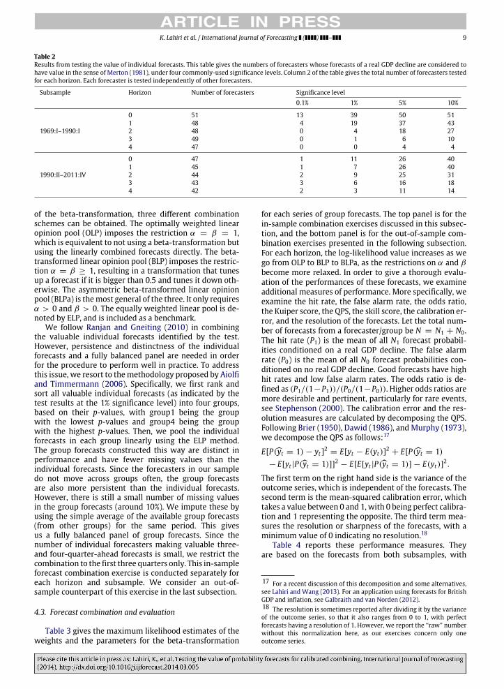
With the aimof constructing a better series of combinedforecasts based only on the valuable individual forecasts,we test the value of the forecasts for each individualforecaster who satisfies the participation requirement.The forecasts for each horizon and subsample from eachindividual are tested separately from the rest. For horizonsh = 0 to 4, for a given level of significance, the numbers offorecasters whose forecasts are considered to have valuein the sense of Merton (1981) are given in Table 2.14
14 We report only the results from the zH test, since the results from thez J test are quite similar. The omitted results are available from the authorson request.
Depending on the subsample, at 1% significance level,23% to 75% of the forecasters make valuable forecastsfor the current quarter. It is clear that the number offorecasters making valuable forecasts decreases sharplyafter two quarters (i.e., the current and the next quarter).After the third quarter, only a few forecasters are makingvaluable forecasts, but a significantly larger proportion offorecasters make valuable forecasts in subsample 2 thanin subsample 1. Surprisingly, beyond two quarters, lessthan 10% of the forecasters make valuable forecasts forsubsample 1,while around 20%of the forecasters stillmakevaluable forecasts for subsample 2. This could be due tothe later period having much less volatility in real GDP,except for the short period around the 2008 recession.Note that the aforementioned observations are made eventhough almost all of the individual series look reasonablygood whenmeasured by QPS, as is shown in Table 1.15 Ourresults are consistent with what has been reported in theliterature about the performance of the SPF forecasts (forexample, Lahiri & Wang, 2013; Stark, 2010).
4.2. Beta-transformed linear pool
It is widely accepted that combining forecasts leadsto higher accuracy. With a rich data set containing anabundance of individual series of forecasts like the SPF,forecast combination should prove to be helpful. In fact,many studies have shown that a significant performanceboost can be obtained by combining survey forecasts prop-erly.16 However, Ranjan and Gneiting (2010) show thatany non-trivially weighted average of two or more dis-tinct and calibrated probability forecasts must be uncal-ibrated and lack sharpness (i.e., have a low resolution).They propose to apply a beta-transformation to the lin-early combined probability forecasts in order to restorecalibration and resolution. Letpit be the probability fore-cast made by forecaster i for time t . The beta-transformedcombined forecastpt takes the formpt = Hα,β(
i wipit),
where Hα,β(p) = B(α, β)−1 p0 tα−1(1 − t)β−1dt for p ∈
[0, 1]. α > 0 and β > 0 are the shape parameters forthe cumulative distribution function of the beta transfor-mation. The log-likelihood function can then be writtenas l =
t yt ln[Hα,β(
i wipit)] +
t(1 − yt) ln[1 −
Hα,β(
i wipit)], where yt is the binary variable to beforecast. Ranjan and Gneiting (2010) suggest estimatingthe parameters of the beta-transformation along with theweights for linear combination by maximum likelihood.Depending on the restrictions imposed on the parameters
15 Following Seillier-Moiseiwitsch and Dawid (1993), we also testwhether the forecasts are perfect, in the sense that QPS is notunreasonably larger than its expected value of
ft (1− ft ), using the test
statistic Yn =
Tt=1(1−2ft )(xt−ft )
[T
t=1(1−2ft )2(1−ft )ft ]1/2→d N(0, 1). We find that everyone
passes the test except for a very few forecasters at long horizons. Thisapparent lack of power may be due to the fact that the test does notexplicitly accommodate serial correlation and skewness.16 For recent examples using the ECB and the US SPF data, see Genre,Kenny, Meyler, and Timmermann (2010) and Lahiri et al. (2012) respec-tively. Clements (2011) studies the properties of various combinationschemes for a number of plausible data generating processes.
K. Lahiri et al. / International Journal of Forecasting ( ) – 9
Table 2Results from testing the value of individual forecasts. This table gives the numbers of forecasters whose forecasts of a real GDP decline are considered tohave value in the sense of Merton (1981), under four commonly-used significance levels. Column 2 of the table gives the total number of forecasters testedfor each horizon. Each forecaster is tested independently of other forecasters.
Subsample Horizon Number of forecasters Significance level0.1% 1% 5% 10%
1969:I–1990:I
0 51 13 39 50 511 48 4 19 37 432 48 0 4 18 273 49 0 1 6 104 47 0 0 4 4
1990:II–2011:IV
0 47 1 11 26 401 45 1 7 26 402 44 2 9 25 313 43 3 6 16 184 42 2 3 11 14
of the beta-transformation, three different combinationschemes can be obtained. The optimally weighted linearopinion pool (OLP) imposes the restriction α = β = 1,which is equivalent to not using a beta-transformation butusing the linearly combined forecasts directly. The beta-transformed linear opinion pool (BLP) imposes the restric-tion α = β ≥ 1, resulting in a transformation that tunesup a forecast if it is bigger than 0.5 and tunes it down oth-erwise. The asymmetric beta-transformed linear opinionpool (BLPa) is themost general of the three. It only requiresα > 0 and β > 0. The equally weighted linear pool is de-noted by ELP, and is included as a benchmark.
We follow Ranjan and Gneiting (2010) in combiningthe valuable individual forecasts identified by the test.However, persistence and distinctness of the individualforecasts and a fully balanced panel are needed in orderfor the procedure to perform well in practice. To addressthis issue, we resort to themethodology proposed by Aiolfiand Timmermann (2006). Specifically, we first rank andsort all valuable individual forecasts (as indicated by thetest results at the 1% significance level) into four groups,based on their p-values, with group1 being the groupwith the lowest p-values and group4 being the groupwith the highest p-values. Then, we pool the individualforecasts in each group linearly using the ELP method.The group forecasts constructed this way are distinct inperformance and have fewer missing values than theindividual forecasts. Since the forecasters in our sampledo not move across groups often, the group forecastsare also more persistent than the individual forecasts.However, there is still a small number of missing valuesin the group forecasts (around 10%). We impute these byusing the simple average of the available group forecasts(from other groups) for the same period. This givesus a fully balanced panel of group forecasts. Since thenumber of individual forecasters making valuable three-and four-quarter-ahead forecasts is small, we restrict thecombination to the first three quarters only. This in-sampleforecast combination exercise is conducted separately foreach horizon and subsample. We consider an out-of-sample counterpart of this exercise in the last subsection.
4.3. Forecast combination and evaluation
Table 3 gives the maximum likelihood estimates of theweights and the parameters for the beta-transformation
for each series of group forecasts. The top panel is for thein-sample combination exercises discussed in this subsec-tion, and the bottom panel is for the out-of-sample com-bination exercises presented in the following subsection.For each horizon, the log-likelihood value increases as wego from OLP to BLP to BLPa, as the restrictions on α and βbecome more relaxed. In order to give a thorough evalu-ation of the performances of these forecasts, we examineadditional measures of performance. More specifically, weexamine the hit rate, the false alarm rate, the odds ratio,the Kuiper score, the QPS, the skill score, the calibration er-ror, and the resolution of the forecasts. Let the total num-ber of forecasts from a forecaster/group be N = N1 + N0.The hit rate (P1) is the mean of all N1 forecast probabil-ities conditioned on a real GDP decline. The false alarmrate (P0) is the mean of all N0 forecast probabilities con-ditioned on no real GDP decline. Good forecasts have highhit rates and low false alarm rates. The odds ratio is de-fined as (P1/(1−P1))/(P0/(1−P0)). Higher odds ratios aremore desirable and pertinent, particularly for rare events,see Stephenson (2000). The calibration error and the res-olution measures are calculated by decomposing the QPS.Following Brier (1950), Dawid (1986), and Murphy (1973),we decompose the QPS as follows:17
E[P(yt = 1) − yt ]2 = E[yt − E(yt)]2 + E[P(yt = 1)− E[yt |P(yt = 1)]]2 − E[E[yt |P(yt = 1)] − E(yt)]2.
The first term on the right hand side is the variance of theoutcome series, which is independent of the forecasts. Thesecond term is the mean-squared calibration error, whichtakes a value between 0 and 1, with 0 being perfect calibra-tion and 1 representing the opposite. The third term mea-sures the resolution or sharpness of the forecasts, with aminimum value of 0 indicating no resolution.18
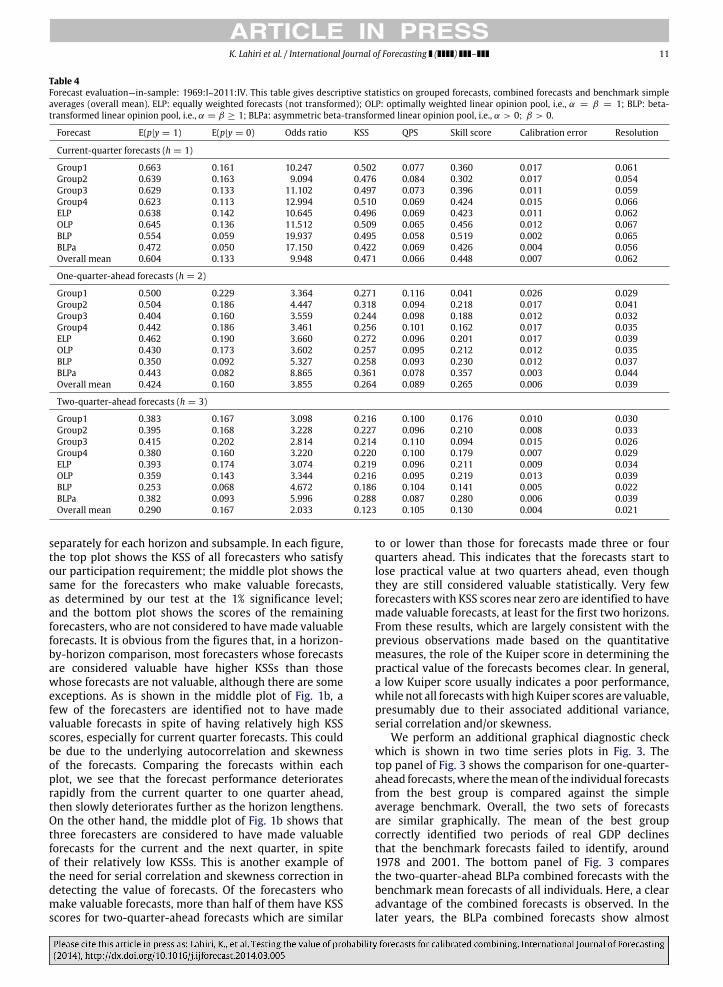
Table 4 reports these performance measures. Theyare based on the forecasts from both subsamples, with
17 For a recent discussion of this decomposition and some alternatives,see Lahiri and Wang (2013). For an application using forecasts for BritishGDP and inflation, see Galbraith and van Norden (2012).18 The resolution is sometimes reported after dividing it by the varianceof the outcome series, so that it also ranges from 0 to 1, with perfectforecasts having a resolution of 1. However, we report the ‘‘raw’’ numberwithout this normalization here, as our exercises concern only oneoutcome series.

10 K. Lahiri et al. / International Journal of Forecasting ( ) –
Table 3Estimated parameters for a beta-transformed linear combination of group forecasts. This table gives the log-likelihood value, estimated weights for eachseries of group forecasts, and estimated parameters α and β for the beta-transformation. OLP: optimally weighted linear opinion pool, i.e., α = β = 1;BLP: beta-transformed linear opinion pool, i.e., α = β ≥ 1; BLPa: asymmetric beta-transformed linear opinion pool, i.e., α > 0; β > 0.
Subsample Horizon Method Log-likelihood w1 w2 w3 w4 alpha beta
In-sample exercise
1969:I–1990:I
0OLP −22.25 0.82 0.00 0.18 0.00 1.00 1.00BLP −22.09 0.79 0.00 0.21 0.00 1.19 1.19BLPa −22.08 0.78 0.00 0.22 0.00 1.18 1.14
1OLP −32.24 0.00 0.00 0.56 0.44 1.00 1.00BLP −31.78 0.32 0.00 0.39 0.28 1.24 1.24BLPa −28.77 0.00 0.93 0.07 0.00 1.48 1.50
2OLP −32.33 0.47 0.00 0.00 0.53 1.00 1.00BLP −31.21 0.06 0.62 0.00 0.33 1.22 1.22BLPa −31.16 0.02 0.65 0.00 0.33 1.12 1.02
1990:II–2011:IV
0OLP −18.21 0.33 0.00 0.67 0.00 1.00 1.00BLP −11.01 0.20 0.00 0.40 0.40 3.59 3.59BLPa −8.84 0.30 0.00 0.23 0.47 3.39 1.84
1OLP −22.21 0.00 0.33 0.67 0.00 1.00 1.00BLP −16.66 0.03 0.00 0.97 0.00 3.08 3.08BLPa −10.81 0.67 0.00 0.33 0.00 3.73 1.50
2OLP −20.13 0.51 0.23 0.00 0.25 1.00 1.00BLP −13.65 0.00 0.67 0.00 0.33 3.72 3.72BLPa −12.43 0.00 0.67 0.00 0.33 6.64 9.87
Out-of-sample exercise
1979:I–1990:I
0OLP −12.33 0.00 0.67 0.33 0.00 1.00 1.00BLP −11.76 0.40 0.40 0.20 0.00 1.00 1.00BLPa −10.57 0.40 0.40 0.20 0.00 1.34 0.82
1OLP −19.19 0.00 0.00 0.67 0.33 1.00 1.00BLP −18.33 0.51 0.00 0.48 0.00 1.00 1.00BLPa −17.36 0.00 0.33 0.00 0.67 0.67 0.29
2OLP −14.62 0.23 0.32 0.45 0.00 1.00 1.00BLP −14.40 0.00 0.37 0.64 0.00 1.33 1.33BLPa −13.91 0.27 0.55 0.17 0.00 0.76 0.39
the second subsample appended to the end of the firstsubsample. Here, we evaluate the four group forecasts,the combined forecasts under different restrictions onthe beta-transformation, and the benchmark forecasts,i.e., the simple average of all individual forecasts (overallmean) in the original SPF data without the participationrequirement imposed. In general, the group forecastsoutperform the average individual forecasts,19 and thecombined forecasts outperform both the group and theaverage individual forecasts. Comparing the four groupforecasts across the different performance measures, wefind that a low p-value from the test does not imply a betterperformance across all of the measures, which is hardlysurprising. In fact, we do not find any single measure tobe sufficient in determining the quality of the forecasts.Looking at the performances of the combined forecasts,we find that even though the beta-transformation reducesthe calibration error onlymodestly, the combined forecastsproduced by the BLP and the BLPa methods do havemuch higher odds ratios than those produced by theOLP or ELP methods. This is especially true for longerhorizon forecasts. For two-quarter-ahead forecasts, theBLPa combined forecasts have an odds ratio of 6.0, whichis almost double that of the ELP forecasts, at 3.1. Moreover,the beta-transformed combined forecasts seem to have a
19 Statistics for individual forecasts for each subsample separately areomitted for brevity, but are available from the authors.
better performance than the average forecasts of all theindividuals at longer horizons. The BLPa combined two-quarter-ahead forecasts performed best according to six ofthe seven measures. In addition, in terms of the odds ratio,the Kuiper score, and the QPS, the BLPa two-quarter-aheadcombined forecasts are better than all four group means.
We test for calibration of the simple average and BLPacombined forecasts using the prequential test of Seillier-Moiseiwitsch and Dawid (1993) (SM-D). Lahiri and Wang(2013) report the results of this test using the overallaverage probabilities. Since many of the original proba-bility intervals contain very few observations, followingSM-D’s guideline to ensure an adequate number of ob-servations in each interval, we consolidate the elevenprobability bins into only three groups, and compute thecalibration test statistic for each forecast horizon. The cal-culated χ2 values are such that the linear opinion poolforecasts for all of the quarters are found to be uncali-brated at the usual 5% level of significance with 2 degreesof freedom. However, as designed by Ranjan and Gneiting(2010), the BLPa forecasts are found to be calibrated. Un-fortunately, due to the sparseness of observations in thehigher probability bins, we cannot make any inference oncalibration at higher deciles of forecast probabilities. Ourtest results are reported in Table 5.
4.4. Additional graphical diagnostics
As has been described, Figs. 1a and 1b show rankedindividual KSS scores for three groups of forecasters,
K. Lahiri et al. / International Journal of Forecasting ( ) – 11
Table 4Forecast evaluation—in-sample: 1969:I–2011:IV. This table gives descriptive statistics on grouped forecasts, combined forecasts and benchmark simpleaverages (overall mean). ELP: equally weighted forecasts (not transformed); OLP: optimally weighted linear opinion pool, i.e., α = β = 1; BLP: beta-transformed linear opinion pool, i.e., α = β ≥ 1; BLPa: asymmetric beta-transformed linear opinion pool, i.e., α > 0; β > 0.
Forecast E(p|y = 1) E(p|y = 0) Odds ratio KSS QPS Skill score Calibration error Resolution
Current-quarter forecasts (h = 1)
Group1 0.663 0.161 10.247 0.502 0.077 0.360 0.017 0.061Group2 0.639 0.163 9.094 0.476 0.084 0.302 0.017 0.054Group3 0.629 0.133 11.102 0.497 0.073 0.396 0.011 0.059Group4 0.623 0.113 12.994 0.510 0.069 0.424 0.015 0.066ELP 0.638 0.142 10.645 0.496 0.069 0.423 0.011 0.062OLP 0.645 0.136 11.512 0.509 0.065 0.456 0.012 0.067BLP 0.554 0.059 19.937 0.495 0.058 0.519 0.002 0.065BLPa 0.472 0.050 17.150 0.422 0.069 0.426 0.004 0.056Overall mean 0.604 0.133 9.948 0.471 0.066 0.448 0.007 0.062
One-quarter-ahead forecasts (h = 2)
Group1 0.500 0.229 3.364 0.271 0.116 0.041 0.026 0.029Group2 0.504 0.186 4.447 0.318 0.094 0.218 0.017 0.041Group3 0.404 0.160 3.559 0.244 0.098 0.188 0.012 0.032Group4 0.442 0.186 3.461 0.256 0.101 0.162 0.017 0.035ELP 0.462 0.190 3.660 0.272 0.096 0.201 0.017 0.039OLP 0.430 0.173 3.602 0.257 0.095 0.212 0.012 0.035BLP 0.350 0.092 5.327 0.258 0.093 0.230 0.012 0.037BLPa 0.443 0.082 8.865 0.361 0.078 0.357 0.003 0.044Overall mean 0.424 0.160 3.855 0.264 0.089 0.265 0.006 0.039
Two-quarter-ahead forecasts (h = 3)
Group1 0.383 0.167 3.098 0.216 0.100 0.176 0.010 0.030Group2 0.395 0.168 3.228 0.227 0.096 0.210 0.008 0.033Group3 0.415 0.202 2.814 0.214 0.110 0.094 0.015 0.026Group4 0.380 0.160 3.220 0.220 0.100 0.179 0.007 0.029ELP 0.393 0.174 3.074 0.219 0.096 0.211 0.009 0.034OLP 0.359 0.143 3.344 0.216 0.095 0.219 0.013 0.039BLP 0.253 0.068 4.672 0.186 0.104 0.141 0.005 0.022BLPa 0.382 0.093 5.996 0.288 0.087 0.280 0.006 0.039Overall mean 0.290 0.167 2.033 0.123 0.105 0.130 0.004 0.021
separately for each horizon and subsample. In each figure,the top plot shows the KSS of all forecasters who satisfyour participation requirement; the middle plot shows thesame for the forecasters who make valuable forecasts,as determined by our test at the 1% significance level;and the bottom plot shows the scores of the remainingforecasters, who are not considered to havemade valuableforecasts. It is obvious from the figures that, in a horizon-by-horizon comparison, most forecasters whose forecastsare considered valuable have higher KSSs than thosewhose forecasts are not valuable, although there are someexceptions. As is shown in the middle plot of Fig. 1b, afew of the forecasters are identified not to have madevaluable forecasts in spite of having relatively high KSSscores, especially for current quarter forecasts. This couldbe due to the underlying autocorrelation and skewnessof the forecasts. Comparing the forecasts within eachplot, we see that the forecast performance deterioratesrapidly from the current quarter to one quarter ahead,then slowly deteriorates further as the horizon lengthens.On the other hand, the middle plot of Fig. 1b shows thatthree forecasters are considered to have made valuableforecasts for the current and the next quarter, in spiteof their relatively low KSSs. This is another example ofthe need for serial correlation and skewness correction indetecting the value of forecasts. Of the forecasters whomake valuable forecasts, more than half of them have KSSscores for two-quarter-ahead forecasts which are similar
to or lower than those for forecasts made three or fourquarters ahead. This indicates that the forecasts start tolose practical value at two quarters ahead, even thoughthey are still considered valuable statistically. Very fewforecasters with KSS scores near zero are identified to havemade valuable forecasts, at least for the first two horizons.From these results, which are largely consistent with theprevious observations made based on the quantitativemeasures, the role of the Kuiper score in determining thepractical value of the forecasts becomes clear. In general,a low Kuiper score usually indicates a poor performance,while not all forecastswith highKuiper scores are valuable,presumably due to their associated additional variance,serial correlation and/or skewness.
We perform an additional graphical diagnostic checkwhich is shown in two time series plots in Fig. 3. Thetop panel of Fig. 3 shows the comparison for one-quarter-ahead forecasts,where themean of the individual forecastsfrom the best group is compared against the simpleaverage benchmark. Overall, the two sets of forecastsare similar graphically. The mean of the best groupcorrectly identified two periods of real GDP declinesthat the benchmark forecasts failed to identify, around1978 and 2001. The bottom panel of Fig. 3 comparesthe two-quarter-ahead BLPa combined forecasts with thebenchmark mean forecasts of all individuals. Here, a clearadvantage of the combined forecasts is observed. In thelater years, the BLPa combined forecasts show almost
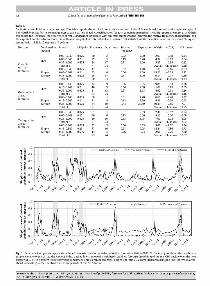
12 K. Lahiri et al. / International Journal of Forecasting ( ) –
Table 5Calibration test: BLPa vs. simple average. This table reports the results from a calibration test of the BLPa combined forecasts and simple averages ofindividual forecasts for the current quarter to two quarters ahead. At each horizon, for each combination method, the table reports the intervals and theirmidpoints, the frequency, the occurrence of real GDP declines for periods with forecasts falling into the intervals, the relative frequency of occurrence, andthe expected number of occurrences, as well as the weight of the interval and all associated test statistics. At 5%, the critical value for the overall Chi squaretest statistic is 5.99 for 2 degrees of freedom.
Horizon Combinationmethod
Interval Midpoint Frequency Occurrence Relativefrequency
Expectation Weight N(0, 1) Chi square
Current-quarterforecasts
BLPa
0.00–0.049 0.025 120 2 0.02 3.00 2.93 −0.58 0.340.05–0.349 0.2 27 5 0.19 5.40 4.32 −0.19 0.040.35–1.000 0.675 24 17 0.71 16.20 5.27 0.35 0.12Total of 3 171 24 Overall Chi square 0.50
Simpleaverage
0.00–0.049 0.025 47 1 0.02 1.18 1.15 −0.16 0.030.05–0.349 0.2 95 6 0.06 19.00 15.20 −3.33 11.120.35–1.000 0.675 28 17 0.61 18.90 6.14 −0.77 0.59Total of 3 170 24 Overall Chi square 11.73
One-quarter-aheadforecasts
BLPa
0.00–0.149 0.075 142 9 0.06 10.65 9.85 −0.53 0.280.15–0.249 0.2 10 3 0.30 2.00 1.60 0.79 0.630.25–1.000 0.625 21 12 0.57 13.13 4.92 −0.51 0.26Total of 3 173 24 Overall Chi square 1.16
Simpleaverage
0.00–0.149 0.075 96 1 0.01 7.20 6.66 −2.40 5.770.15–0.249 0.2 31 4 0.13 6.20 4.96 −0.99 0.980.25–1.000 0.625 44 19 0.43 27.50 10.31 −2.65 7.01Total of 3 171 24 Overall Chi square 13.75
Two-quarter-aheadforecasts
BLPa
0.00–0.049 0.025 101 1 0.01 2.53 2.46 −0.97 0.940.05–0.249 0.15 40 6 0.15 6.00 5.10 0.00 0.000.25–1.000 0.625 30 16 0.53 18.75 7.03 −1.04 1.08Total of 3 171 23 Overall Chi square 2.02
Simpleaverage
0.00–0.149 0.075 82 3 0.04 6.15 5.69 −1.32 1.740.15–0.349 0.25 77 16 0.21 19.25 14.44 −0.86 0.730.35–1.000 0.696 14 5 0.36 9.74 2.96 −2.76 7.60Total of 3 173 24 Overall Chi square 10.07
Fig. 3. Benchmark simple averages and combined forecasts based on valuable individual forecasts—1969:I–2011:IV. The top figure shows the benchmarksimple average forecasts (i.e., the Anxious Index, dashed line) and equally weighted combined forecasts (solid line) of the real GDP decline over the nextquarter (h = 1). The bottom figure shows the benchmark simple average forecasts (dashed line) and BLPa combined forecasts (solid line) for two-quarter-ahead forecasts (h = 2). The shaded areas are periods of real GDP decline.
K. Lahiri et al. / International Journal of Forecasting ( ) – 13
uniformly better performance, i.e., the forecasts are highduring periods with real GDP declines and low during non-decline periods, except for a few quarters around mid-2001. In the earlier years, except perhaps for the 1978period, the BLPa combined forecasts also perform betterthan the benchmark.
These observations echo the results presented inTable 4 and confirm the reasonable quality of the simpleaverage benchmark forecasts. However, more importantly,they also show the superiority of the beta-transformedoptimally-weighted forecasts, which are based on theforecasters who make valuable forecasts, as identified bythe test. We note that it may seem from the number offorecasters making valuable forecasts (as shown in Table 2and the graphical checks, especially Fig. 3) as though mostforecasters perform better in general in the later years,covered by subsample 2. Using a fixed benchmark forecastthatmatches the overall sample proportion of periodswitha real GDP decline, we can compute the skill scores for eachof the subsample periods. The results show that, except forthe current quarter forecasts (where they turn out to bealmost the same), the forecastsmade during the later yearsdo indeed display higher skill levels.
4.5. An out-of-sample evaluation
As was shown in the previous subsection, the improve-ment in the forecasting performance which is attributedto combining only the valuable forecasts, as identified bythe test, demonstrates its usefulness. While the purposeof the test is merely to assess a given set of forecasts anddetermine its value, it would be more useful if the testcould help with out-of-sample forecast combination. Toexplore this possibility, we adapt the procedure used in thein-sample forecast combination exercise in the previoussection for performing out-of-sample combination. Specif-ically, we use the part of the first subsample from 1969:I to1978:IV as the training sample, and test each forecaster’sperformance during this period.20 The forecasters that arefound to have made valuable forecasts during the train-ing sample period are retained for combination using theevaluation sample from 1979:I to 1990:I. The combinedforecasts for this out-of-sample period are then evaluatedusing the same set of performancemeasures as used in theprevious exercise.
Before we discuss the results, several remarks on thesetup of this exercise are in order. First, in order to eval-uate the value of the forecasts properly using the test, thetrack record of a forecastermust cover sufficiently long pe-riods of both real GDP declines and real GDP growth. Asthere are only three episodes of real GDP declines in thesecond subsample, the issue ofmissing datameans that notenough observations are available for most forecasters ifthe subsample is further divided into a training sample andan evaluation sample. Therefore, in our out-of-sample ex-ercise, only subsample 1 is considered. Second, it is compu-tationally feasible to apply the test to either an expanding
20 The training sample is selected so as to leave enough observationsof both real GDP declines and real GDP growth in both the training andevaluation samples.
window of forecasts or a rolling window of forecasts, thusallowing the testing and forecast combination procedureto be carried out in real time. However, for the majority ofthe periods in which there is no real GDP decline, addingonemore observation to the training sample does not alterthe test result. This dissuades us from attempting a real-time combination and evaluation, since the conclusionswewould obtain from a real time implementation could alsobe obtained from a simple out-of-sample exercise. Third,the crucial element of a successful combination of forecastsis that a forecaster’s past performance is a good predictorof her future performance. Obviously, this is a data-specificproperty and is not related to forecast combination proce-dures. Therefore, one should avoid interpreting the perfor-mance of the combined forecasts as the performance of thetest, even though, in general, a more powerful test shouldhelp to produce better combined forecasts.
The estimated combination weights are reported in thebottompanel of Table 3, and the performancemeasures arereported in Table 6. For current-quarter forecasts, the ELPand OLP combined forecasts outperform the overall meanbenchmark in terms of most of the performance mea-sures. This indicates the ability of the test to identify goodforecasters out-of-sample, based on their track record.However, for longer horizon forecasts, even though thecombined forecasts are marginally better than the bench-mark, neither the combined forecasts nor the benchmarkappear to display any skill. This suggests the basic unpre-dictability of the target variable at longer horizons. Thiscould also be due to the fact that the evaluation sample pe-riod is very volatile, with frequent real GDP declines thatare difficult to foresee. We again note that, since the pre-dictability of forecasters’ performances is a key ingredientof successful forecast combination, it is unlikely that the re-sults reported here can be generalized readily to other vari-ables and data sets, even though the empirical strategy andprocedure used here should be of value more generally.
5. Concluding remarks
In order to identify the forecasters whose forecastshave ‘‘no value’’ in a KSS sense (or in the sense of Mer-ton, 1981), we propose the use of a serial correlationand skewness-robust Welch-type test that utilizes theprobability forecasts directly, without requiring the fore-casts to be converted to binary forecasts before testing.Wethen test, combine, and analyze in detail the probabilityforecasts of a real GDP decline using data from the US Sur-vey of Professional Forecasters from 1968Q4 to 2012Q1.While the data set spans more than four decades cover-ing many recessions and cyclical downturns, it contains alarge number of missing values. In order to mitigate thisproblem,we follow themulti-stepmethodology suggestedby Aiolfi and Timmermann (2006), by first sorting the fre-quent forecasters into four clusters based on their past per-formances, then applying the BLP methodology of Ranjanand Gneiting (2010) to these clusters in order to obtaincalibrated combined forecasts. We compare the combinedforecasts based on the valuable individual forecasts to thesimple average (ELP) of all of the forecasts for current-,one-, and two-quarter horizons.
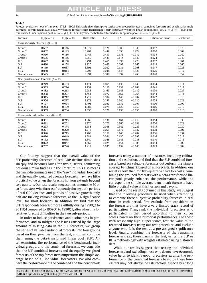
14 K. Lahiri et al. / International Journal of Forecasting ( ) –
Table 6Forecast evaluation—out-of-sample: 1979:I–1990:I. This table gives descriptive statistics on grouped forecasts, combined forecasts and benchmark simpleaverages (overall mean). ELP: equally weighted forecasts (not transformed); OLP: optimally weighted linear opinion pool, i.e., α = β = 1; BLP: beta-transformed linear opinion pool, i.e., α = β ≥ 1; BLPa: asymmetric beta-transformed linear opinion pool, i.e., α > 0; β > 0.
Forecast E(p|y = 1) E(p|y = 0) Odds ratio KSS QPS Skill score Calibration error Resolution
Current-quarter forecasts (h = 1)
Group1 0.667 0.146 11.677 0.521 0.086 0.345 0.017 0.070Group2 0.632 0.143 10.267 0.489 0.096 0.274 0.020 0.064Group3 0.596 0.186 6.445 0.410 0.133 −0.012 0.033 0.040Group4 0.595 0.156 7.959 0.439 0.114 0.136 0.024 0.049ELP 0.622 0.158 8.791 0.465 0.095 0.278 0.017 0.061OLP 0.620 0.158 8.720 0.462 0.097 0.265 0.018 0.060BLP 0.119 0.037 3.501 0.082 0.131 0.008 0.017 0.026BLPa 0.050 0.014 3.793 0.036 0.148 −0.123 0.026 0.017Overall mean 0.575 0.187 5.894 0.388 0.097 0.260 0.020 0.057
One-quarter-ahead forecasts (h = 2)
Group1 0.249 0.183 1.474 0.065 0.138 −0.049 0.014 0.011Group2 0.333 0.224 1.734 0.110 0.158 −0.201 0.041 0.017Group3 0.382 0.213 2.285 0.169 0.146 −0.112 0.039 0.027Group4 0.298 0.227 1.451 0.072 0.167 −0.268 0.044 0.011ELP 0.315 0.212 1.717 0.104 0.143 −0.087 0.022 0.013OLP 0.354 0.217 1.972 0.137 0.146 −0.110 0.033 0.022BLP 0.127 0.094 1.408 0.033 0.132 −0.001 0.006 0.009BLPa 0.214 0.139 1.683 0.075 0.125 0.050 0.006 0.015Overall mean 0.359 0.234 1.839 0.126 0.138 −0.050 0.020 0.016
Two-quarter-ahead forecasts (h = 3)
Group1 0.351 0.215 1.969 0.136 0.164 −0.419 0.054 0.036Group2 0.421 0.251 2.170 0.170 0.160 −0.382 0.036 0.022Group3 0.263 0.174 1.688 0.088 0.142 −0.225 0.015 0.020Group4 0.271 0.220 1.318 0.051 0.177 −0.532 0.038 0.007ELP 0.326 0.215 1.768 0.111 0.148 −0.282 0.036 0.034OLP 0.080 0.049 1.684 0.031 0.150 −0.297 0.016 0.012BLP 0.132 0.085 1.649 0.048 0.143 −0.238 0.010 0.013BLPa 0.072 0.047 1.565 0.025 0.151 −0.308 0.014 0.009Overall mean 0.262 0.226 1.212 0.035 0.132 −0.140 0.023 0.009
Our findings suggest that the overall value of theSPF probability forecasts of real GDP decline diminishessharply and becomes low after two quarters, confirmingprevious similar findings in the literature. This also meansthat an indiscriminate use of the ‘‘raw’’ individual forecastsand the equally weighted average forecasts may have littlepractical value when the forecast horizon extends beyondtwo quarters. Our test results suggest that, among the 50 orso forecasters who forecast frequently during both periodsof real GDP declines and periods of positive growth, onlyhalf are making valuable forecasts, at the 1% significancelevel, for short horizons. In addition, we find that theSPF respondents forecast more skillfully during 1990Q2 to2011Q4 compared to 1969Q1 to 1990Q1, after adjusting forrelative forecast difficulties in the two sub-periods.
In order to induce persistence and distinctness in per-formance, and to mitigate the issues caused by the largeamount of missing data in the SPF forecasts, we groupthe series of valuable individual forecasts into four groupsbased on their p-values from the test, and then combinethem using the beta-transformed linear pool (BLP). Af-ter examining the performance of the benchmark, indi-vidual groups, and the combined forecasts, we concludethat the BLP combined forecasts and the equally-weightedforecasts of the top forecasters outperform the simple av-erage based on all individual forecasters. We also com-pare the performance of the combined and the benchmark
forecasts using a number of measures, including calibra-tion and resolution, and find that the ELP combined fore-casts based on valuable forecasts outperform the simpleaverage benchmark based on all forecasts. In addition, ourresults show that, for two-quarter-ahead forecasts, com-bining the grouped forecasts with a beta-transformed lin-ear pool greatly enhances the performance, while thecorresponding simple average benchmark forecasts havelittle practical value at this horizon and beyond.
Based on the results obtained in this study, we suggestthat the following procedure be used when attemptingto combine these subjective probability forecasts in realtime. In each period, first exclude from considerationthe forecasters that have a very limited track record ofparticipation. Then, rank the individual forecasters whoparticipated in that period according to their Kuiperscores based on their historical performances. For thosewith reasonably high Kuiper scores, test the value of therecorded forecasts using our test procedure, and excludeanyone who fails the test at a pre-assigned significancelevel. Finally, combine the forecasts of the remainingforecasters, i.e., those passing the test, using the BLP orBLPamethodologywithweights estimated using historicaldata.
While our results suggest that testing the individualforecasters and excluding thosewho do not have economicvalue helps to identify good forecasters ex ante, the per-formance of the combined forecasts based on these fore-casters may not always be satisfactory, especially at long
K. Lahiri et al. / International Journal of Forecasting ( ) – 15
horizons. This is due to the fact that the ex ante fore-cast performance of individual forecasters is highly data-dependent, and is unrelated to the empirical method thatwe choose to compare them. Nevertheless, the test pro-posed in this paper provides an additional dimension alongwhich the economic value of potentially serially correlatedand skewed forecasts can be assessed, independent of anythreshold parameter that would be required to convert theprobabilities to binary forecasts.
Acknowledgments
This research was supported by the National Instituteon Minority Health and Health Disparities, NationalInstitutes of Health (grant number 1 P20 MD003373).The content is solely the responsibility of the authorsand does not represent the official views of the NationalInstitute on Minority Health and Health Disparities or theNational Institutes of Health. The authors thank, withoutimplicating, the anonymous referee and Prakash Lounganifor their helpful comments.
Appendix. Technical proofs
Definition:
Sk,Tri =1Ti
Tit=1
Ep∗3it +
3Ti
Tris=1
Tit=s+1
Ep∗2
i,tp∗
i,t−s
+
3Ti
Tris=1
Tit=s+1
Ep∗
i,tp∗2i,t−s
+
6Ti
Triτ=1
Tris=τ+1
Tit=s+1
Ep∗
i,tp∗
i,t−τp∗
i,t−s
Sk,Tri =
1Ti
Tit=1
p∗3it +
3Ti
Tris=1
ω(s, Tri)Ti
t=s+1
p∗2i,tp∗
i,t−s
+3Ti
Tris=1
ω(s, Tri)Ti
t=s+1
p∗
i,tp∗2i,t−s
+6Ti
Triτ=1
ω(τ, Tri)Tri
s=τ+1
ω(s, Tri)p∗
i,tp∗
i,t−τp∗
i,t−s.
Lemma 1. Under Assumption A,√Tipi − pi
→p N
0, σ 2
i
as Ti → ∞.
Proof. See Corollary 5.3(ii) in Hall and Heyde (1980). �
Lemma 2. Suppose Assumptions A and B hold. Then Sk,i =
limTi→∞ Sk,Ti < ∞, and Sk,Tri − Sk,Ti → 0 as Ti → ∞.
Proof. By definition,
Sk,Ti =1Ti
Tit=1
Ep∗3i,t +
3Ti
Ti−1s=1
Tit=s+1
Ep∗2
i,tp∗
i,t−s
+
3Ti
Ti−1s=1
Tit=s+1
Ep∗
i,tp∗2i,t−s
+
6Ti
Ti−2τ=1
Ti−1s=τ+1
Tit=s+1
Ep∗
i,tp∗
i,t−τp∗
i,t−s
,
sincep∗
i,t = pi,t − pi andpi,t is stationary with Epi,t = pi,
and Epi,t 8+δ
≤ D < ∞ for some δ > 0. It followsimmediately that 1
Ti
Tit=1 Ep∗3
i,t = Ep∗3i,t < ∞. Next, by
using the fact that Ep∗
i,t−s = 0 and Corollary 6.16 of White(1984), we obtain
Ep∗2
i,tp∗
i,t−s
= E
(p∗2
i,t − Ep∗2i,t )p∗
i,t−s
≤ [αi(s)]
δ2+2δ M
for some positive finiteM . Hence,
3Ti
Ti−1s=1
Tit=s+1
E p∗2i,tp∗
i,t−s
≤3Ti
Ti−1s=1
Tit=s+1
[αi(s)]δ
2+2δ M
= 3MTi−1s=1
[αi(s)]δ
2+2δ
Ti − sTi
≤ 3MTi−1s=1
[αi(s)]δ
2+2δ
< ∞,
because αi(s) is of size (2 + 2δ)/δ. Similarly, we have
3Ti
Ti−1s=1
Tit=s+1
E p∗
i,tp∗2i,t−s
< ∞.
Turning to the term 6Ti
Ti−2τ=1
Ti−1s=τ+1
Tit=s+1 E
p∗
i,tp∗
i,t−τp∗
i,t−s
, where 0 < τ < s, it can be seen that
6Ti
Ti−2τ=1
Ti−1s=τ+1
Tit=s+1
Ep∗
i,tp∗
i,t−τp∗
i,t−s
≤ 6M
Ti−2τ=1
Ti−1s=τ+1
[αi(s)αi(τ )]δ
2+2δ
Ti − sTi
< 6MTi−2τ=1
[αi(τ )]δ
2+2δ
Ti−1s=1
[αi(s)]δ
2+2δ
< ∞.
Thus, Sk,Ti is bounded above for all Ti, so limTi→∞ Sk,Ti existsand limTi→∞ Sk,Ti < ∞. The proof of Sk,Tri − Sk,Ti → 0 asTi → ∞parallels exactly the proof of Lemma6.17 ofWhite(1984), and hence is omitted here. �
Proposition 1. Under Assumptions A and B,Sk,Tri →p Sk,i asTi → ∞ for i = 0, 1, where Sk,i = limTi→∞ Sk,Ti .
Proof. By Lemma 1,
pi,t =p∗
i,t + (pi − pi) =p∗
i,t + Op
1
T 1/2i
, (9)
which, along with the stationarity of p∗
i,t , implies thatSk,Tri =Sk,Tri+Op
1
T1/2i
. Since Sk,Ti−Sk,Tri → 0 as Ti → ∞
and Sk,i = limTi→∞ Sk,Ti , by virtue of Lemma 2, it suffices toshowSk,Tri − Sk,Tri →p 0 as Ti → ∞. By triangle inequality,
16 K. Lahiri et al. / International Journal of Forecasting ( ) –
Sk,Tri − Sk,Tri ≤
1TiTi
t=1
p∗3it − Ep∗3
it
+
3Ti
Tris=1
|ω(s, Tri) − 1|Ti
t=s+1
E(p∗2i,tp∗
i,t−s)
+3Ti
Tris=1
|ω(s, Tri) − 1|Ti
t=s+1
E(p∗
i,tp∗2i,t−s)
+
6Ti
Triτ=1
ω(τ, Tri)Tri
s=τ+1
|ω(s, Tri) − 1|
×
Tit=s+1
E(p∗
i,tp∗
i,t−τp∗
i,t−s)+ 6
Ti
Triτ=1
|ω(τ, Tri) − 1|
×
Tris=τ+1
ω(s, Tri)Ti
t=s+1
E(p∗
i,tp∗
i,t−τp∗
i,t−s)
+6Ti
Triτ=1
|ω(τ, Tri) − 1|Tri
s=τ+1
|ω(s, Tri) − 1|
×
Tit=s+1
E(p∗
i,tp∗
i,t−τp∗
i,t−s)
+
3TiTris=1
ω(s, Tri)Ti
t=s+1
p∗2i,tp∗
i,t−s − E(p∗2i,tp∗
i,t−s)
+
3TiTri−1s=1
ω(s, Tri)Ti
t=s+1
p∗
i,tp∗2i,t−s − E(p∗
i,tp∗2i,t−s)
+
6TiTri
τ=1
ω(τ, Tri)Tri
s=τ+1
ω(s, Tri)Ti
t=s+1
[p∗
i,tp∗
i,t−τp∗
i,t−s
− E(p∗
i,tp∗
i,t−τp∗
i,t−s)]
.Sincepi,t is stationary and has αi(t) of size (2 + 2δ)/δ andEp4+δ
i,t < ∞ for some δ > 0, by Theorem 2.10 of Mcleish(1975), we have
1Ti
Tit=1
Ep∗3i,t →p. Ep∗3
i,t < ∞,
so that the first term goes to zero. Next, as was shownin Lemma 2, we have
E(p∗2i,tp∗
i,t−s) ≤ [αi(s)]
δ2+2δ M for
some finite constant M . Hence, 1Ti
Tit=s+1
E(p∗2i,tp∗
i,t−s) ≤
[αi(s)]δ
2+2δ M for all Ti and s. Sinceω(s, Tri) = 1−s
Tri+1 → 1for each s, the second term tends to zero as Ti → 0, byvirtue of the dominated convergence theorem. By simi-lar arguments, the third, fourth, fifth and sixth terms allapproach zero as Ti → 0. Next, let ztτ s =p∗
i,tp∗
i,t−τp∗
i,t−s −
E(p∗
i,tp∗
i,t−τp∗
i,t−s); then, it follows immediately from As-sumption A that Ez2+2δ
tτ s ≤ D∗ < ∞ for some constant D∗
and δ > 0. Then, using an argument similar to that in The-orem 2 of Newey and West (1987), we obtain
E
Ti
t=s+1
Eztτ s
2
≤ (Ti − s) (s + 1)∆ ≤ Ti(s + 1)∆
for s > 0 and some ∆ < ∞. Hence,
P
1TiTri
τ=1
ω(τ, Tri)Tri
s=τ+1
ω(s, Tri)Ti
t=s+1
Eztτ s
> ε
≤ P
1Ti
Triτ=1
ω(τ, Tri)Tri
s=τ+1
ω(s, Tri)
Ti
t=s+1
Eztτ s
> ε
≤
Triτ=1
Tris=τ+1
P
1TiTi
t=s+1
Eztτ s
>ε
2Tri(Tri − 1)
≤
Triτ=1
Tris=τ+1
E
1Ti
Tit=s+1
Eztτ s
2
ε
2Tri(Tri−1)
2≤
4T 2ri(Tri − 1)2
Tiε2∆
Triτ=1
Tris=1
(s + 1)
=2T 4
ri(Tri − 1)2(Tri + 2)Tiε2
→ 0,
provided T7riTi
→ 0. That is, the ninth term goes to zero if T 7ri
grows more slowly than T . By a similar argument, the sev-enth and eighth terms also go to zero under Assumptions Aand B. Therefore, we can conclude thatSk,Tri − Sk,Tri
→p 0,
which completes the proof. �
References
Aiolfi, M., & Timmermann, A. (2006). Persistence in forecasting perfor-mance and conditional combination strategies. Journal of Economet-rics, 135(1–2), 31–53.
Braun, P., & Yaniv, I. (1992). A case study of expert judgment: economists’probabilities versus base rate model forecasts. Journal of BehavioralDecision Making , 5, 217–231.
Brier, G. (1950). Verification of forecasts expressed in terms ofprobability.Monthly Weather Review, 78, 1–3.
Capistran, C., & Timmermann, A. (2009). Forecast combinationwith entryand exit of experts. Journal of Business and Economic Statistics, 27(4),428–440.
Clements, M. P. (2008). Consensus and uncertainty: using forecastprobabilities of output declines. International Journal of Forecasting ,24, 76–86.
Clements, M. P. (2009). Internal consistency of survey respondents’forecasts: evidence based on the Survey of Professional Forecasters.In J. L. Castle, N. Shephard, D. F. Hendry, J. Castle, & N. Shephard (Eds.),The methodology and practice of econometrics (pp. 206–226). Oxfordand New York: Oxford University Press.
Clements, M. P. (2011). An empirical investigation of the effects ofrounding on the SPF probabilities of decline and output growthhistograms. Journal of Money, Credit and Banking , 43(1), 207–220.
Clements, M. P., & Harvey, D. I. (2010). Forecast encompassing testsand probability forecasts. Journal of Applied Econometrics, 25(6),1028–1062.
Clements, M., & Harvey, D. I. (2011). Combining probability forecasts.International Journal of Forecasting , 27(2), 208–223.
Croushore, D. (1993). Introducing: the Survey of Professional Forecasters.Federal Reserve Bank of Philadelphia Business Review, 3–13.
Dawid, A. (1986). Probability forecasting. In Encyclopedia of statisticalsciences.
Engelberg, J., Manski, C., & Williams, J. (2010). Assessing the temporalvariation of macroeconomic forecasts by a panel of changingcomposition. Journal of Applied Econometrics, 26(7), 1059–1078.
K. Lahiri et al. / International Journal of Forecasting ( ) – 17
Galbraith, J. W., & van Norden, S. (2011). Kernel-based calibration diag-nostics for recession and inflation probability forecasts. InternationalJournal of Forecasting , 27(4), 1041–1057.
Galbraith, J. W., & van Norden, S. (2012). Assessing gross domesticproduct and inflation probability forecasts derived from Bank ofEngland fan charts. Journal of the Royal Statistical Society, Series A(Statistics in Society), 175, 713–727.
Genre, V., Kenny, G., Meyler, A., & Timmermann, A. (2010). Combiningexpert forecasts: can anything beat the simple average? InternationalJournal of Forecasting , 27(2), 108–121.
Graham, H. R. (1996). Is a group of forecasters better than one? Journal ofBusiness, 69(2), 193–232.
Granger, C.W. J., & Pesaran,M. H. (2000). A decision theoretic approach toforecast evaluation. In W.-S. Chan, W. K. Li, & H. Tong (Eds.), Statisticsand finance (pp. 261–278). London and River Edge and NJ: ImperialCollege Press and Distributed by World Scientific Pub.
Guo, J. H., & Luh, W. M. (2000). An invertible transformation two-sampletrimmed t-statistic under heterogeneity and nonnormality. Statistics& Probability Letters, 49, 1–7.
Hall, P. (1992). On the removal of skewness by transformation. Journal ofthe Royal Statistical Society, Series B, 54, 221–228.
Hall, P., & Heyde, C. (1980). Martingale limit theory and its applications.New York: Academic Press.
Henriksson, R. D., & Merton, R. C. (1981). On market timing andinvestment performance, II: Satistical procedures for evaluatingforecasting skills. Journal of Business, 54(4), 513–533.
Johnson, N. J. (1978). Modified t-tests and confidence intervals for asym-metrical populations. Journal of the American Statistical Association, 73,536–544.
Lahiri, K., Monokroussos, G., & Zhao, Y. (2013). The yield spread puzzleand the information content of SPF forecasts. Economics Letters, 118,219–221.
Lahiri, K., Peng, H., & Zhao, Y. (2012). Forecast combination in incompletepanels. Department of Economics Working Paper, University atAlbany-SUNY.
Lahiri, K., & Wang, J. G. (2006). Subjective probability forecasts forrecessions: guidelines for use. Business Economics, 41(2), 26–37.
Lahiri, K., & Wang, J. G. (2013). Evaluating probability forecasts for GDPdeclines using alternative methodologies. International Journal ofForecasting , 29, 175–190.
Luh, W. M., & Guo, J. H. (1999). A powerful transformation trimmedmean method for one way fixed effects ANOVA model under non-normality and inequality of variances. British Journal of Mathematicaland Statistical Psychology, 52, 303–320.
Mcleish, D. L. (1975). A maximal in equality and dependent strong laws.Annals of Probability, 3, 829–839.
Merton, R. C. (1981). Onmarket timing and investment performance, I: Anequilibrium theory of value for market forecasts. Journal of Business,54(3), 363–406.
Murphy, A. (1973). A new vector partition of the probability score. Journalof Applied Meteorology, 12, 595–600.
Newey, W. K., & West, K. D. (1987). A simple, positive semi-definite,heteroskedasticity and autocorrelation consistent covariancematrix.Econometrica, 55, 703–708.
Newey, W. K., &West, K. D. (1994). Automatic lag selection in covarianceestimation. Review of Economic Studies, 61, 631–654.
Pesaran, M. H., & Timmermann, A. (1992). A simple nonparametric testof predictive performance. Journal of Business and Economic Statistics,10, 461–465.
Pesaran, M. H., & Timmermann, A. (1994). A generalization of the non-parametric Henriksson–Merton test of market timing. EconomicsLetters, 44(1–2), 1–7.
Pesaran, M. H., & Timmermann, A. (2009). Testing dependence amongserially correlated multicategory variables. Journal of the AmericanStatistical Association, 104, 325–337.
Ranjan, R., & Gneiting, T. (2010). Combining probability forecasts. Journalof the Royal Statistical Society, Series B (Statistical Methodology), 72(1),71–91.
Rudebusch, G. D., & Williams, J. C. (2009). Forecasting recessions: thepuzzle of the enduring power of the yield curve. Journal of Businessand Economic Statistics, 27, 492–503.
Schnader, M. H., & Stekler, H. O. (1990). Evaluating predictions of change.Journal of Business, 63(1), 99–107.
Seillier-Moiseiwitsch, F., & Dawid, A. P. (1993). On testing the validityof sequential probability forecasts. Journal of the American StatisticalAssociation, 88(421), 355–359.
Sohn, K. T., & Park, S. M. (2008). Guidance on the choice of thresholdfor binary forecast modeling. Advances in Atmospheric Sciences, 25(1),83–88.
Stark, T. (2010). Realistic evaluation of real-time forecasts in the Surveyof Professional Forecasters. Federal Reserve Bank of PhiladelphiaResearch Special Report.
Stekler, H. O. (1994). Are economic forecasts valuable? Journal ofForecasting , 13, 495–505.
Stephenson, D. B. (2000). Use of the odds ratio for diagnosing forecastskill.Weather and Forecasting , 15, 221–232.
Stock, J. H., &Watson, M.W. (2003). Forecasting output and inflation: therole of asset prices. Journal of Economic Literature, 41, 788–829.
White, H. (1984). Asymptotic theory for econometricians. New York:Academic Press.
Kajal Lahiri is a distinguished professor of economics at the Universityat Albany-SUNY, a fellow of CESifo Research Network, and an honoraryfellow of the International Institute of Forecasters. He received hisdoctorate in economics from the University of Rochester. Author ofnumerous books and articles, Dr. Lahiri created the TransportationServices Index, a measure of output in the transportation sector thatis reported monthly by the US Department of Transportation. He ison the editorial boards of the Journal of Econometrics, the InternationalJournal of Forecasting, Empirical Economics, and the Journal of BusinessCycleMeasurement and Analysis. His current research dealswith economicforecasting, and also with minority health, with the latter research beingfunded by the National Institutes of Health.
Huaming Peng (Ph.D., Yale University) is Assistant Professor of eco-nomics at the Department of Economics of SUNY at Albany. His researchinterests include theoretical and applied econometrics, and time seriesforecasting.
Yongchen Zhao is a doctoral candidate at the Department of Economics,the University at Albany-SUNY. His research interests are in the areasof forecasting, applied econometrics, and finance. His recent work hascentered on forecasting with survey data and many predictors, includingissues in forecast combination, forecast evaluation and testing, as well asapplications to the hedge fund industry.