Embed Size (px)
Citation preview

Testing the Mediated Effect in the Pretest-Posttest Control Group Design
by
Matthew John Valente
A Thesis Presented in Partial Fulfillment
of the Requirements for the Degree
Master of Arts
Approved February 2015 by the
Graduate Supervisory Committee:
David MacKinnon, Chair
Stephen West
Leona Aiken
Craig Enders
ARIZONA STATE UNIVERSITY
May 2015

i
ABSTRACT
Methods to test hypotheses of mediated effects in the pretest-posttest control group
design are understudied in the behavioral sciences (MacKinnon, 2008). Because many
studies aim to answer questions about mediating processes in the pretest-posttest control
group design, there is a need to determine which model is most appropriate to test
hypotheses about mediating processes and what happens to estimates of the mediated
effect when model assumptions are violated in this design. The goal of this project was
to outline estimator characteristics of four longitudinal mediation models and the cross-
sectional mediation model. Models were compared on type 1 error rates, statistical
power, accuracy of confidence interval coverage, and bias of parameter estimates. Four
traditional longitudinal models and the cross-sectional model were assessed. The four
longitudinal models were analysis of covariance (ANCOVA) using pretest scores as a
covariate, path analysis, difference scores, and residualized change scores. A Monte
Carlo simulation study was conducted to evaluate the different models across a wide
range of sample sizes and effect sizes. All models performed well in terms of type 1
error rates and the ANCOVA and path analysis models performed best in terms of bias
and empirical power. The difference score, residualized change score, and cross-
sectional models all performed well given certain conditions held about the pretest
measures. These conditions and future directions are discussed.

ii
DEDICATION
This document is dedicated to my family and my girlfriend for their continued support.

iii
ACKNOWLEDGMENTS
I thank my committee chair, David MacKinnon, and the rest of my committee for their
help in the creation and execution of this project. Lastly, I thank my friends, family, and
girlfriend for their support.

iv
TABLE OF CONTENTS
Page
LIST OF TABLES……………………………………………………………………iv
LIST OF FIGURES……………………………………………………………….….vi
INTRODUCTION………………………………………………………………….....1
Statistical Mediation………………………………………………………1
Pretest-Posttest Control Group Design……………………………………3
Pretest-Posttest Control Group Design with a Mediating Variable……….4
Analysis of Change in Mediation Models and Conditions to be Met…….7
Hypotheses……………………………………………………………….14
METHOD…………………………………………………………………................15
RESULTS…………………………………………………………………................26
DISCUSSION…………………………………………………………......................62
Implications………………………………………………………………66
Limitations……………………………………………………………….68
Future Directions……………………………………………………...…70
REFERENCES...……………………………………………………….……………74

v
APPENDIX Page
A LIST OF VARIABLE NAMES AND DESCRIPTIONS……………………127
B LIST OF MODEL COEFFICIENTS AND DESCRIPTIONS………………129
C SAS MACRO FOR DATA-GENERATION…………...……………………131
D FIGURE OF DATA-GENERATING MODEL………...……………………134
E ESTIMATED QUANTITIES AND MODEL CONDITIONS….………...…136
F SAS MACRO FOR ANALYSIS OF ALL MODELS….……………………138
G SAS MACRO FOR CALLING PRODCLIN TO ESTIMATE CONFIDENCE
INTERVALS FOR THE MEDIATED EFFECT FOR THE ANCOVA
MODEL…………….……………………………………...…………………163
H SAS MACRO CREATING PERCENTILE BOOTSTRAPPED CONFIDENCE
INTERVALS FOR ALL MODELS……………..…..….………...…………165
I SAS MACRO FOR SUMMARIZING RESULTS ACROSS ALL MODELS
FOR USE IN ANOVA FOR RESULTS SECTION………............……….…173

vi
APPENDIX Page
J SAS MACRO FOR SUMMARIZING PRODCLIN RESULTS FOR USE IN
ANOVA FOR RESULTS SECTION………...………………………..…...…176
K SAS MACRO FOR SUMMARIZING RESULTS BY AVERAGING ACROSS
REPLICATIONS FOR USE IN TABLES FOR RESULTS SECTION…….182
L FIGURE OF CROSS-SECTIONAL MODEL……………………………….185
M FIGURE OF DIFFERENCE SCORE MODEL..…………...…………….....187
N FIGURE OF RESIDUALIZED CHANGE SCORE MODEL………………189
O COVARIANCE ALGEBRA…………………………………………………191
P TRUE CORRELATIONS……………………………………………………201

vii
LIST OF TABLES
Table Page
1. All Combinations of Effect Size Adopted from MacKinnon, Lockwood, and
Williams (2004)………………………………………………………………….83
2. PRODCLIN Type 1 Error Rates for N = 50……………………………………..84
3. PRODCLIN Type 1 Error Rates for N = 100………………...………………….84
4. PRODCLIN Type 1 Error Rates for N = 200……………………...…………….85
5. PRODCLIN Type 1 Error Rates for N = 500…………...……………………….85
6. Bias, Relative Bias, and Standardized Bias of the Mediated Effect for the
ANCOVA Model………………………………………………………………...86
7. Bias, Relative Bias, and Standardized Bias of the Mediated Effect for the Path
Analysis Model……………….…………………………………………..……...87
8. Bias, Relative Bias, and Standardized Bias of the Mediated Effect for the
Difference Score Model..…………………………..………………………….....88
9. Bias, Relative Bias, and Standardized Bias of the Mediated Effect for the
Residualized Change Score Model When Pretest Correlation = 0.00....………...89
10. Bias, Relative Bias, and Standardized Bias of the Mediated Effect for the
Residualized Change Score Model When Pretest Correlation = 0.50…………...90
11. Bias, Relative Bias, and Standardized Bias of the Mediated Effect for the Cross-
Sectional Model When Direct Effect = 0.00……………....………......................91
12. Bias, Relative Bias, and Standardized Bias of the Mediated Effect for the Cross-
Sectional Model When Direct Effect = 0.30 and N = 50..……….........................92

viii
Table Page
13. Bias, Relative Bias, and Standardized Bias of the Mediated Effect for the Cross-
Sectional Model When Direct Effect = 0.30 and N = 100……………….............92
14. Bias, Relative Bias, and Standardized Bias of the Mediated Effect for the Cross-
Sectional Model When Direct Effect = 0.30 and N = 200……………………….93
15. Bias, Relative Bias, and Standardized Bias of the Mediated Effect for the Cross-
Sectional Model When Direct Effect = 0.30 and N = 500……………………….93
16. PRODCLIN 95% Confidence Interval Coverage of the Mediated Effect for the
ANCOVA Model………………………………………………………………...94
17. PRODCLIN 95% Confidence Interval Coverage of the Mediated Effect for the
Path Analysis Model……………………………………………………………..94
18. PRODCLIN 95% Confidence Interval Coverage of the Mediated Effect for
Difference Score Model………………………………………………………….95
19. PRODCLIN 95% Confidence Interval Coverage of the Mediated Effect for
Residualized Change Score Model When Direct Effect = 0.00, N = 50, and N =
100.....………………………………………………………………...…...….….96
20. PRODCLIN 95% Confidence Interval Coverage of the Mediated Effect for
Residualized Change Score Model When Direct Effect = 0.00, N = 200, and N =
500....……………………………………………………………………....…….97
21. PRODCLIN 95% Confidence Interval Coverage of the Mediated Effect for
Residualized Change Score Model When Direct Effect = 0.30, N = 50, and N =
100………………………………………………………………………………..98

ix
Table Page
22. PRODCLIN 95% Confidence Interval Coverage of the Mediated Effect for
Residualized Change Score Model When Direct Effect = 0.30, N = 200, and N =
500....…….……......………………………………………………………….…..99
23. PRODCLIN 95% Confidence Interval Coverage of the Mediated Effect for Cross-
Sectional Model When Direct Effect = 0.00……………...…………………….100
24. PRODCLIN 95% Confidence Interval Coverage of the Mediated Effect for Cross-
Sectional Model When Direct Effect = 0.30………...………………………….100
25. Comparison of Sample Size Requirement for 0.80 Power to Detect the Cross-
Sectional Mediated Effect Across Current Study and Fritz & MacKinnon
(2007)…………………………………………………………………………...101
26. Significance Test Summary Indicator of the Mediated Effect for the Five
Models…………………………………………………………………………..102

x
LIST OF FIGURES
Figure Page
1. Path Diagram of Pretest - Posttest Control Group Design With Mediating
Variable…………………………………………………………………………103
2. Power Plot of ANCOVA Model Mediated Effect Results by Sample Size and
Effect Size Collapsed Across All Simulation Conditions………………………104
3. Power Plot of ANCOVA Model Mediated Effect Results by Sample Size and
Effect Size Collapsed Across All Simulation Conditions....................................105
4. Power Plot of Difference Score Model Mediated Effect Results by Sample Size,
Effect Size, and Stability Collapsed Across All Simulation Conditions.............106
5. Power Plot of Residualized Change Score Model Mediated Effect Results by
Sample Size, Effect Size, bm2y1 Path and Direct Effect = 0.00 Collapsed Across
All Simulation Conditions...................................................................................107
6. Power Plot of Residualized Change Score Model Mediated Effect Results by
Effect Size, bm2y1 Path, by2m1 Path for Sample Size N = 50 and N = 100 and
Direct Effect = 0.30 Collapsed Across All Simulation Conditions....................108
7. Power Plot of Residualized Change Score Model Mediated Effect Results by
Effect Size, bm2y1 Path, by2m1 Path for Sample Size N = 200 and N = 500 and
Direct Effect = 0.30 Collapsed Across All Simulation Conditions....................109
8. Power Plot of Cross-Sectional Model Mediated Effect Results by Sample Size
and Effect Size for Direct Effect = 0.00 Collapsed Across All Simulation
Conditions………………………………………………………….…………...110

xi
Figure Page
9. Power Plot of Cross-Sectional Model Mediated Effect Results by Sample Size
and Effect Size for Direct Effect = 0.30 Collapsed Across All Simulation
Conditions…………………………………………………………………........111
10. Power Plot of ANCOVA VS. Cross-Sectional Model Mediated Effect Results by
Sample Size and Effect Size Collapsed Across All Simulation Conditions........112
11. Power Plot of Path Analysis VS. Cross-Sectional Model Mediated Effect Results
by Sample Size and Effect Size Collapsed Across All Simulation Conditions...113
12. Power Plot of Difference Score VS. Cross-Sectional Model Mediated Effect
Results by Effect Size, Stability, and by2m1 Path for Sample Size N = 50 and N =
100 and Direct Effect = 0.00 Collapsed Across All Simulation Conditions.......114
13. Power Plot of Difference Score VS. Cross-Sectional Model Mediated Effect
Results by Effect Size, Stability, and by2m1 Path for Sample Size N = 200 and N
= 500 and Direct Effect = 0.00 Collapsed Across All Simulation Conditions....115
14. Power Plot of Difference Score VS. Cross-Sectional Model Mediated Effect
Results by Effect Size and Stability for Direct Effect = 0.30 Collapsed Across All
Simulation Conditions……………………………………….…………………116
15. Power Plot of Residualized Change Score VS. Cross-Sectional Model Mediated
Effect Results by Sample Size and Effect Size Collapsed Across All Simulation
Conditions………………………………………………………………………117

xii
Figure Page
16. Power Plot of Path Analysis VS. Difference Score Model Mediated Effect Results
by Sample Size, Effect Size, Stability, and by2m1 Path for Sample Size N = 50
and N = 100 and Direct Effect = 0.00 Collapsed Across All Simulation
Conditions……………………………………………………………………....118
17. Power Plot of Path Analysis VS. Difference Score Model Mediated Effect Results
by Sample Size, Effect Size, Stability, and by2m1 Path for Sample Size N = 200
and N = 500 and Direct Effect = 0.00 Collapsed Across All Simulation
Conditions……………………………………………………………………... 119
18. Power Plot of Path Analysis VS. Difference Score Model Mediated Effect Results
by Sample Size, Effect Size, Stability, bm2y1 Path, and by2m1 Path for Sample
Size N = 50 and Direct Effect = 0.30 Collapsed Across All Simulation
Conditions………………………………………………………………………120
19. Power Plot of Path Analysis VS. Difference Score Model Mediated Effect Results
by Sample Size, Effect Size, Stability, bm2y1 Path, and by2m1 Path for Sample
Size N = 100 and Direct Effect = 0.30 Collapsed Across All Simulation
Conditions...... ......... ......... ......... ......... ......... ......... ......... ......... ....................121
20. Power Plot of Path Analysis VS. Difference Score Model Mediated Effect Results
by Sample Size, Effect Size, Stability, bm2y1 Path, and by2m1 Path for Sample
Size N = 200 and Direct Effect = 0.30 Collapsed Across All Simulation
Conditions........... ......... ......... ......... ......... ......... ......... ......... ......... ...............122

xiii
Figure Page
21. Power Plot of Path Analysis VS. Difference Score Model Mediated Effect Results
by Sample Size, Effect Size, Stability, bm2y1 Path, and by2m1 Path for Sample
Size N = 500 and Direct Effect = 0.30 Collapsed Across All Simulation
Conditions........... ........... ........... ........... ........... ........... ........... ........... ............123
22. Power Plot of Path Analysis VS. Residualized Change Score Model Mediated
Effect Results by Sample Size, Effect Size, Stability, bm2y1 Path, and by2m1 Path
for Sample Size N = 50 and N = 100 Collapsed Across All Simulation
Conditions...... ........... ........... ........... ........... ........... ........... .............................124
23. Power Plot of Path Analysis VS. Residualized Change Score Model Mediated
Effect Results by Sample Size, Effect Size, Stability, bm2y1 Path, and by2m1 Path
for Sample Size N = 200 and N = 500 Collapsed Across All Simulation
Conditions...... ........... ........... ........... ........... ........... ........... ........... .................125
24. Multidimensional Scaling Using Tetrachoric Correlations to Categorize the Power
to Detect the Mediated Effect for the Five Models on Two
Dimensions…………………………..................................................................126

1
Introduction
Many research designs consist of two-waves of measurement and aim to test
mediation hypotheses. A PsycINFO search of the terms “two-wave or pretest posttest or
two time points” and “mediation or mediating or mediator or process variable” during the
span 2000 – 2014 resulted in 485 peer-reviewed articles. There are four commonly used
models to test mediated effects in the pretest-posttest control group design: Analysis of
covariance (ANCOVA), Path analysis, difference score, and residualized change score.
Additionally, it is possible to estimate the mediated effect using a cross-sectional model
that ignores the pretest information on both the mediator and the outcome variable.
Given the wide use of these models in mediation analysis, it is surprising that few studies
have evaluated under what conditions these models have don’t type 1 error rates above
the nominal 0.05 alpha level, produce unbiased estimates of the mediated effect, have
confidence interval coverage that is close to 95%, and have high empirical power to
detect the mediated effect. This project aims to compare tests of the mediated effect in
the pretest-posttest control group design using these four common traditional longitudinal
models and the cross-sectional model.
Statistical Mediation
Most research focuses on assessing relations between two variables, with the
research question of whether or not there is a total effect of an independent variable X on
a dependent variable Y (Sobel, 1990). Additional variables can be included to further
investigate how or why there is a relation between the two variables. When variables are
added to bivariate relations, these additional variables can result in a variety of third

2
variable effects including confounding, moderating, or mediating effects. Of particular
interest in this project are third variables that are defined as mediating variables. A
mediating variable is a variable that is both a dependent variable and an independent
variable and is intermediate in a causal sequence between two variables (Lazarsfeld,
1955; MacKinnon, 2008; Sobel 1990). Inclusion of a mediating variable in a theoretical
model and statistical analyses allows researchers to test indirect effects of an independent
variable on a dependent variable through the independent variable’s effect on the
mediating variable (Lazarsfeld, 1955; MacKinnon, 2008; Sobel 1990).
Statistical mediation is important because it allows researchers to investigate how
two variables are related. Once researchers know two variables are related (e.g., X
causes Y) it may be of theoretical interest to investigate through what mechanism X and
Y are related. Statistical mediation is a tool by which causal mechanisms can be
investigated given assumptions (MacKinnon, 2008; VanderWeele & Vansteelandt, 2009).
Statistical mediation is typically conceptualized using a series of three linear regression
equations (MacKinnon, 2008). Equation 1 represents the total effect of X on Y (c
coefficient), Equation 2 represents the effect of X on M (a coefficient), and Equation 3
represents the effect of X on Y adjusted for M (c’ coefficient) and the effect of M on Y
adjusted for X (b coefficient). Computing the product of a and b coefficients from
Equation 2 and Equation 3, respectively, represents the indirect effect of X on Y through
M (ab).
𝑌 = 𝑖1 + 𝑐𝑋 + 𝑒1 (1)
𝑀 = 𝑖2 + 𝑎𝑋 + 𝑒2 (2)

3
𝑌 = 𝑖3 + 𝑐′𝑋 + 𝑏𝑀1 + 𝑒3 (3)
These three linear regression equations are used to assess statistical mediation in cross-
sectional experimental designs. A cross-sectional experimental design is one which
researchers measure variables at a single time point. Longitudinal experimental designs
are ones in which researchers measure variables over time or treatment effects at a later
time point (Shadish, Cook, & Campbell, 2002). One type of longitudinal design that
incorporates a randomized experiment is the pretest-posttest control group design
(Bonate, 2002; Shadish, Cook, & Campbell, 2002).
Pretest-Posttest Control Group Design
The pretest-posttest control group design is common in a wide range of research
areas. This design consists of randomly assigning units to either a control group or a
treatment group, measuring theoretically relevant variables before delivery of a treatment,
and then measuring these same variables again at a later point in time after treatment
(Bonate, 2002; Shadish, Cook, & Campbell, 2002). Random assignment of units to
treatment and initial measurement of variables occur at the pretest stage of an
experiment. Variables are measured again at the posttest stage of an experiment after
delivery of a treatment to the treatment group. This document describes the two groups
as the treatment and control groups but the control condition may actually be a standard
treatment or some other comparison for the treatment investigated.
Pretest-posttest control group designs can assess how much change, or gain, in
scores on measured variables has occurred for the treatment and control group between
pretest and posttest. Because this design allows researchers to measure variables twice

4
for each unit, and units are randomly assigned to different treatment groups, researchers
can answer questions about within-group changes between pretest and posttest and
between-group differences in change between pretest and posttest (Bonate, 2002;
Shadish, Cook, & Campbell, 2002).
The timing of posttest measurement is an important aspect of experimental design
and should be determined a priori and based on previous research. If timing of posttest
measurement does not match timing of a true effect, estimates of this true effect across
pretest and posttest will typically underestimate the actual true effect (Cohen, 1991;
Collins & Graham, 1991, 2002). In reality, it may be difficult to know exactly when a
true effect is going to occur, and it is likely that true effects will diminish with time after
the true effect occurs (Collins & Graham, 2002). Because predicting timing effects can
be difficult, researchers are often advised to take many repeated measures occurring at
short time intervals (Cohen, 1991; Collins & Graham, 1991, 2002). This project assumes
the posttest measurement matches the timing of the true effect.
Pretest-Posttest Control Group Design with A Mediating Variable
The pretest-posttest control group design can be extended to research questions
regarding mediating variables (as shown in Figure 1). When X is a randomized treatment
variable coded zero or one, a common way to assess mediated effects is by estimating a
series of linear regression equations similar to those used to assess mediated effects in
cross-sectional data. Equation 4 represents the effect of X on the mediator measured at
posttest adjusted for pretest mediator (am2x coefficient) and the pretest outcome, the effect
of the mediator measured at pretest (stability) on the mediator measured at posttest (Sm2m1

5
coefficient) adjusted for X and the pretest outcome, and the effect of the outcome
measured at pretest on the mediator measured at posttest (bm2y1 coefficient) adjusted for X
and the pretest mediator. Equation 5 represents the effect of X on the outcome variable
measured at posttest (c’y2x coefficient) adjusted for the other variables in the equation, the
effect of the outcome variable measured at pretest (stability) on the outcome variable
measured at posttest (Sy2y1 coefficient) adjusted for the other variables in the equation, the
effect of the mediator measured at pretest on the outcome variable measured at posttest
(by2m1 coefficient) adjusted for the other variables in the equation, and the effect of the
mediator measured at posttest on the outcome variable measured at posttest (by2m2
coefficient) adjusted for the other variables in the equation (see Appendices A – B for
further explanation of variables and notation).
𝑀2 = 𝑖4 + 𝑎𝑚2𝑥𝑋 + 𝑆𝑚2𝑚1𝑀1 + 𝑏𝑚2𝑦1𝑌1 + 𝑒4 (4)
𝑌2 = 𝑖5 + 𝑐′𝑦2𝑥𝑋 + 𝑆𝑦2𝑦1𝑌1 + 𝑏𝑦2𝑚1𝑀1 + 𝑏𝑦2𝑚2𝑀2 + 𝑒5 (5)
Mediated effects of X on Y2 through M2 in a pretest-posttest design can be
assessed by taking the product of am2x coefficient in Equation 4 and by2m2 coefficient in
Equation 5 (am2xby2m2). This computation of mediated effects in a pretest posttest design
is similar to the computation of mediated effects in cross-sectional designs based on
Equations 1 – 3 except that it includes coefficients from regression equations with pretest
measures as predictors of M and Y at posttest. Equations 4 – 5 correspond to the
ANCOVA or path analysis model and represent all estimable parameters of the
covariance structure in the pretest – posttest control group design with a mediating
variable.

6
The pretest-posttest control group design is the focus of this study because it is
widely used for assessing mediation and little is known about the accuracy of different
models. The pretest – posttest control group design represents the simplest longitudinal
design making it ideal to compare with the commonly-used cross-sectional mediation
design. Several different models have been applied to assess mediation in pretest-posttest
control group designs such as analysis of covariance (Jang, Kim, & Reeve, 2012;
Schmiege, Broaddus, Levin, & Bryan, 2009), path analysis (Cribbie & Jamieson, 2004;
MacKinnon, 2001, 2008), difference scores (Hofmann, 2004; Jansen, et al., 2012;
MacKinnon et al., 1991), and residualized change scores (Cole, Kemeny, Fahey, Zack, &
Naliboff, 2003; Miller, Trost, & Brown, 2002; Reid & Aiken, 2013). The purpose of this
project is to evaluate models to assess mediation in the pretest-posttest control group
design which consists of two time points (i.e., pretest and posttest) assuming that timing
of posttest measurement matches timing of the true effect.
- Insert Figure 1 about here –
Analysis of Change in Mediation Models and Conditions to be Met
Assuming that there is successful randomization of units to the control group and
treatment group so that these groups do not differ systematically at pretest, any observed
change in a unit from the treatment group from pretest to posttest would not have
occurred had that unit been assigned to the control group (Van Breukelen, 2006, 2013).

7
It is also assumed that all measures of pretest and posttest variables in this study are
measured without error. Researchers have expounded on the results of violating these
assumptions using ANCOVA and difference score models outside the context of
mediation (Jamieson, 1999; Kisbu-Sakarya, MacKinnon, & Aiken, 2013; Van Breukelen,
2006, 2013; Wright, 2006).
Cross-sectional model. The cross-sectional model is the simplest of the models because
it does not take into account the pretest measures of the mediator and outcome variable
and therefore does not address a question of change across time. The cross-sectional
model assumes the stabilities of the mediator and the outcome variable are equal to zero,
there is no pretest correlation between the mediator and the outcome, and there are no
cross-lagged relations between the mediator and the outcome or the outcome and the
mediator. Equation 6 represents the relation between the treatment variable and the
posttest mediator (am2x) and Equation 7 represents the relation between the treatment
variable and the posttest outcome (c’y2x) adjusted for the posttest mediator and the
relation between the posttest mediator and the posttest outcome (by2m2) adjusted for the
treatment.
𝑀2 = 𝑖6 + 𝑎𝑚2𝑥𝑋 + 𝑒6 (6)
𝑌2 = 𝑖7 + 𝑐′𝑦2𝑥𝑋 + 𝑏𝑦2𝑚2𝑀2 + 𝑒7 (7)
The cross-sectional mediated effect is estimated by computing the product of am2x
coefficient from Equation 6 and by2m2 coefficient from Equation 7 (am2xby2m2). The cross-
sectional model does not explicitly take into account the pretest measures of the mediator

8
and the outcome in any way. This model assumes there are no relations between the
pretest measures of the mediator and the outcome and no relations between the pretest
measures of the mediator and the outcome and the posttest measures of the mediator and
the outcome.
Difference score model. Difference scores address the question “On average, how much
did each group change across time?” It can be seen that difference scores address a
question of change across time that is unconditional on pretest scores (Dwyer, 1983).
The difference score model assumes the same measure is used at pretest and at posttest
and that the correlation between the prestest and posttest measure (stability) is 1.0
(Bonate, 2002; Campbell & Kenny, 1999; Cronbach & Furby, 1970). Equation 8
represents the difference score that would be calculated for a mediator variable where ΔM
indicates difference in scores on the mediator variable measured at pretest subtracted
from scores on the mediator variable measured at posttest. Equation 9 represents the
difference scores calculated for the outcome variable where ΔY indicates change in scores
on the outcome variable measured at pretest subtracted from scores on the outcome
variable measured at posttest.
∆𝑀= 𝑀2 − 𝑀1 (8)
∆𝑌= 𝑌2 − 𝑌1 (9)
Equations 9 and 10 represent regression equations that are estimated using difference
scores for the mediator variable and outcome variable, respectively.
∆𝑀= 𝑖8 + 𝑎∆𝑋 + 𝑒8 (10)

9
∆𝑌= 𝑖9 + 𝑐′∆𝑋 + 𝑏∆𝛥𝑀 + 𝑒9 (11)
Mediated effects are estimated by computing the product of aΔ coefficient from Equation
10 and bΔ coefficient from Equation 11 (aΔbΔ). When estimating the mediated effect this
way, it becomes clear that the relations between pretest measures of the mediator variable
and the outcome variable are not explicitly taken into account and the cross-lagged
relations between pretest measures and posttest measures are not explicitly taken into
account (pretest mediator to posttest outcome and pretest outcome to posttest mediator).
Therefore, the difference score model in the context of mediation, implicitly assumes
these relations are equal to zero.
Residualized change score model. Residualized change scores are computed by
regressing posttest scores on pretest scores and then computing the difference between
observed posttest scores and predicted posttest scores (residual). No treatment group
variable is included in the regression of posttest scores on pretest scores, which means
posttest scores for units in both treatment groups are adjusted for pretest scores based on
an aggregate of pretest scores across both treatment groups. The residualized change
score model assumes there are no between group differences in the correlation between
the pretest measure and the posttest measure (Cronbach & Furby, 1970). That is, the
correlation between the pretest measure and the posttest measure for the control group is
equal to the correlation between the pretest measure and the posttest measure for the
treatment group.
Residualized change scores answer the question “How different are treatment
group posttest scores given equal treatment group pretest scores?” Residualized change

10
scores address a conditional question of change. That is, given the treatment group and
the control group have equal pretest scores, how different are the treatment group and
control group posttest scores? Equation 12 represents residualized change scores
calculated for the mediator variable, where RM indicates change in predicted scores on the
mediator variable measured at posttest subtracted from observed scores on the mediator
variable measured at posttest. Equation 13 represents residualized change scores
calculated for the outcome variable, where RY indicates change in predicted scores on the
outcome variable measured at posttest subtracted from observed scores on the outcome
variable at posttest.
𝑅𝑀 = 𝑂𝑏𝑠𝑒𝑟𝑣𝑒𝑑 𝑀2 − 𝑃𝑟𝑒𝑑𝑖𝑐𝑡𝑒𝑑 𝑀2 (12)
𝑅𝑌 = 𝑂𝑏𝑠𝑒𝑟𝑣𝑒𝑑 𝑌2 − 𝑃𝑟𝑒𝑑𝑖𝑐𝑡𝑒𝑑 𝑌2 (13)
Equations 13 and 14 represent regression equations that are estimated using residualized
change scores for the mediator variable and the outcome variable, respectively.
𝑅𝑀 = 𝑖10 + 𝑎𝑅𝑋 + 𝑒10 (14)
𝑅𝑌 = 𝑖11 + 𝑐′𝑅𝑋 + 𝑏𝑅𝑅𝑀 + 𝑒11 (15)
Mediated effects are estimated by computing the product of aR coefficient from Equation
14 and bR coefficient from Equation 15 (aRbR). Like the difference score model, the
residualized change score model does not explicitly take into account the pretest
correlation between the mediator and outcome variables and it does not explicitly take
into account the cross-lagged relations. Therefore, this model implicitly assumes these
relations are equal to zero.

11
ANCOVA. ANCOVA is used to assess change by using pretest scores as a covariate
when predicting posttest scores (Bonate, 2002; Campbell & Kenny, 2002). ANCOVA
removes the influence of pretest scores on posttest scores by computing a within-group
regression coefficient of posttest scores on pretest scores for each treatment and control
group, separately. Next, these within group regression coefficients are pooled to form a
single regression coefficient by which posttest scores are adjusted for pretest scores.
ANCOVA specifically addresses the question “On average, how different are the
treatment and control groups scores at posttest given that treatment and control groups
had equivalent pretest scores?” ANCOVA addresses a conditional question of change.
The ANCOVA model assumes that within group regression coefficients are homogenous,
there is no interaction of the covariate (e.g., pretest scores) and the treatment group, and
that the covariate is measured without error (Huitema, 2011; Maxwell & Delaney, 2004).
Equations 15 and 16 represent regression equations that are estimated using ANCOVA to
adjust for pretest scores for the mediator and the outcome variable, respectively.
𝑀2 = 𝑖4 + 𝑎𝑚2𝑥𝑋 + 𝑆𝑚2𝑚1 𝑀1 + 𝑏𝑚2𝑦1𝑌1 + 𝑒4 (16)
𝑌2 = 𝑖5 + 𝑐′𝑦2𝑥𝑋 + 𝑆𝑦2𝑦1 𝑌1 + 𝑏𝑦2𝑚1𝑀1 + 𝑏𝑦2𝑚2𝑀2 + 𝑒5 (17)
Sm2m1 in Equation 16 represents a pooled regression coefficient relating pretest scores
measured on the mediator to posttest scores measured on the mediator within each
treatment and control group and then pooled across both groups. Sy2y1 in Equation 17
represents a pooled regression coefficient relating pretest scores measured on the
outcome variable to posttest scores measured on the outcome variable within each
treatment and control group and then pooled across both groups. Mediated effects are

12
estimated by computing the product of am2x coefficient from Equation 16 and by2m2
coefficient from Equation 17 (am2xby2m2). Unlike the difference score model and the
residualized change score model, the ANCOVA model explicitly takes into account the
cross-lagged relations (as long as they are included in the model equations) and takes into
account the pretest correlation between the mediator and outcome variables because the
predictors in the equations are adjusted for their relations with the other predictors in the
same equation (Cohen, Cohen, West, & Aiken, 2003).
Path analysis. An additional approach to analyzing change in the pretest-posttest control
group design is to analyze the relations specified by equations 16 and 17 using path
analysis. Like the ANCOVA model, path analysis explicitly takes into account the
pretest correlation between the mediator and outcome variables and the cross-lagged
relations (as long they are specified in the model).
Summary. Overall, the cross-sectional, difference score, and residualized change score
model all have specific conditions that need to be met about various model parameters
when testing the mediated effect in the pretest-posttest control group design. None of
these three models take into account any potential pretest correlation between the
mediator and outcome variables and none of the three models directly take into account
any potential cross-lagged relations. The difference score model assumes the stabilities
for the mediator and outcome variables are 1.0 and the cross-sectional model assumes the
stabilities for the mediator and outcome variables are 0.0. The ANCOVA and path
analysis models explicitly estimate or take into account the correlation between the
mediator and outcome at baseline, cross-lagged relations, and stabilities. Therefore, it is

13
expected that the mediated effect estimated with the difference score, residualized change
score, and the cross-sectional model will be biased across a variety of conditions whereas
the mediated effect estimated with the ANCOVA and the path analysis model will not.
The following hypotheses reflect that the performance of the models will be
negatively affected when parameters are non-zero in the true model but are not estimated.
For example, the residualized change score model does not explicitly take into account
any cross-lagged relations between pretest measures and posttest measures therefore
when these relations exist and the residualized change score model is used to estimate the
mediated effect, it is expected that the mediated effect will be biased.
Hypotheses
The first hypothesis is the difference score, residualized change score, ANCOVA,
and path analysis models will perform better than the cross-sectional model in general
because they use the pretest information. The second hypothesis is the cross-sectional,
difference score, and residualized change score models will be biased when either or both
the by2m1 and bm2y1, cross-lagged paths, are non-zero. The third hypothesis is the
cross-sectional, difference score, and residualized change score model will have
confidence interval coverage lower than 95% when either or both the by2m1 or bm2y1
paths are present. The by2m1 and bm2y1 paths are expected to bias the results and lead
to confidence interval coverage lower than 95% for the cross-sectional, difference score,

14
and residualized change score models because these models do not directly take into
account these paths when estimating the mediated effect. The fourth hypothesis is the
cross-sectional, difference score, and residualized change score models will be biased and
have confidence interval coverage lower than 95% when there is a pretest correlation
between the mediator and outcome variables. The presence of the pretest correlation is
expected to bias the results of these models because these models do not take into
account this pretest correlation. The fifth hypothesis is that the difference score model
will have less power when the stability is low versus high because the difference score
model assumes the pretest-posttest correlation (stability) is 1.00. Overall, it is
hypothesized all models will not have type 1 error rates that are greater than the nominal
0.05 alpha level and will have increasing power as effect size of the mediated effect
increases and sample size increases.
The study hypotheses are important because if researchers use the cross-sectional,
difference score, or residualized change score model to estimate mediated effects in the
pretest – posttest control group design, there are specific conditions to be met regarding
the relations between the mediating and outcome variable at the pretest and the relations
of the pretest measures to the posttest measures (i.e., cross-lagged relations). The
conditions range from a zero pretest correlation between the mediator and the outcome to
zero cross-lagged relations between the pretest and posttest measures. It is unlikely that
these conditions are tenable in most research designs and specifically the pretest –
posttest control group design involving mediation effects. The proposed simulation is
designed to investigate how violating these conditions affects the accuracy of the five
models.

15
Method
Data-Generating Model
The SAS 9.3 programming language was used to conduct a Monte Carlo simulation of a
pretest-posttest control group design with a mediating variable. The following equations
represent the data-generating model (see Appendix C) and correspond to the
ANCOVA/path analysis model in the Monte Carlo simulation where 𝑥 is an observed
value of random variable 𝑋 and �̃� is the sample median.
𝑋 ~𝑁(0,1): 𝑥 ≥ �̃� = 1; 𝑥 < �̃� = 0 (34)
𝑀1~𝑁(0,1) (35)
𝑌1 = 𝑏𝑦1𝑚1𝑀1 + 𝑒1 (36)
𝑀2 = 𝑎𝑚2𝑥𝑋 + 𝑏𝑚2𝑦1𝑌1 + 𝑆𝑚2𝑚1𝑀1 + 𝑒2 (37)
𝑌2 = 𝑐′𝑦2𝑥𝑋 + 𝑏𝑦2𝑚1𝑀1 + 𝑏𝑦2𝑚2𝑀2 + 𝑆𝑦2𝑦1𝑌1 + 𝑒3 (38)
𝜎𝑒12 = 1 (39)
𝜎𝑒22 = 1 (40)
𝜎𝑒32 = 1 (41)
𝜎𝑒1𝑒2 = 0 (42)
𝜎𝑒1𝑒3 = 0 (43)
𝜎𝑒2𝑒3 = 0 (44)

16
The Monte Carlo simulation, varied sample size (N = 50, 100, 200, 500), effect
size of the a (am2x) (0 .10, .30, .50), b(by2m2) (0 .10, .30, .50), and c’(c’y2x) (0 and .30)
paths, effect size of the path from the pretest mediator to the posttest outcome (by2m1) (0
and .50), effect size of the path from the pretest outcome to the posttest mediator (bm2y1)
(0 and .50), stability of the mediator (Sm2m1) and the outcome (Sy2y1) (.3 and .7), and the
correlation between the mediator and outcome at pretest (0 and .5). The by1m1 coefficient
in Equation 36 was simulated to be equivalent to a correlation (ρy1m1) of 0 or .5. The
data-generating model diagram (see Appendix D) depicts a causal relation between the
mediator and outcome at pretest but this is to make the Equations 34 – 44 match exactly
with the diagram. That is, although there was a causal arrow relating the mediator at
pretest to the outcome at pretest we will investigate effects of varying the correlation
between these variables and do not assume a unidirectional causal effect between them.
To summarize, 13 combinations of effect sizes for the a, b, and c’ path were
studied. The effect sizes of these paths were all in the correlation metric and chosen to
reflect small, medium, and large effect sizes (Cohen, 1988). The 13 combinations of
effect size were adopted from MacKinnon, Lockwood, and Williams (2004) because they
demonstrated that all other combinations of effect sizes had identical results in their
study. A caveat should be made that the present study differs from the single mediator
model studied in MacKinnon et al. (2004). The combinations are as follows and
summarized in Table 1: a = b = c’=0; a = 0, b = .10, c’ = 0; a = 0, b = .30 c’ = 0; a = 0, b
= .50, c’ = 0; a = .10, b = .10, c’ = 0; a = .30, b = .30, c’ = 0; a = .50, b = .50, c’ = 0; a =
.10, b = .30, c’ = 0; a = .10, b = .50, c’ = 0; a = .30, b = .50, c’ = 0; a = .10, b = .10, c’ =
.30; a = .30, b = .30, c’ = .30; and a = .50, b = .50, c’ = .30. There was 832 conditions

17
defined by 13 effect size combinations, 4 sample sizes, 2 effect sizes of pretest mediator
on posttest outcome, 2 effect sizes or pretest outcome on posttest mediator, 2 stabilities of
mediator and outcome, and 2 correlations between mediator and outcome at pretest. This
resulted in an incomplete factorial design with all factors being fully crossed with one
another except for the last three combinations of effect sizes which included a non-zero
effect size for the c’ path. When this path is non-zero, it is known as a direct effect in the
mediation literature (MacKinnon, 2008). The presence of this direct effect did not occur
for all combinations of effect sizes for the a and b paths. Therefore, the direct effect was
not fully crossed with all the factors in this simulation study. A total of 1,000 replications
of each condition was conducted. The focus of this simulation study was to evaluate
estimator characteristics of the mediated effect (am2x by2m2) for the cross-sectional single
mediator model ignoring the pretest mediator and outcome variables and four
longitudinal models (i.e., difference scores, residualized change scores, ANCOVA, and
path analysis) for assessing change.
Bias of Parameter Estimates
For each replication in each condition, bias of the parameter estimates of the
mediated effect was the parameter estimate minus the true value of the parameter as in
Equation 45. All estimates of bias were averaged over all replications within each
condition.
𝐵𝑖𝑎𝑠(𝜃) = 𝜃 − 𝜃 (45)

18
The relative bias of the parameter estimates of the mediated effect was computed by
dividing the bias of the parameter estimate from Equation 45 by the true value of the
parameter as in Equation 46. All estimates of relative bias were averaged over
replications within each condition.
𝑅𝐵𝑖𝑎𝑠(𝜃) =(�̂�−𝜃)
𝜃 (46)
An estimator was considered acceptable in terms of bias if the absolute value of relative
bias was less than .10 (Flora & Curran, 2004; Kaplan, 1988). One drawback of
calculating relative bias (i.e., Equation 44) is that it cannot be calculated when the true
value of the parameter is equal to zero. To remedy this, the standardized bias (SBias) of
the parameter estimates was computed by dividing the bias of the parameter estimate as
obtained from Equation 45 by the standard deviation of the parameter estimate across
replications (i.e., empirical standard error of the parameter estimate). This measure of
relative bias can be calculated when the true value of the parameter is equal to zero (see
Equation 47). All estimates of standardized bias were averaged over replications within
each condition.
𝑆𝐵𝑖𝑎𝑠(𝜃) =(�̂�−𝜃)
𝑆𝐷�̂� (47)
Significance Testing
Type 1 error rates were the proportion of times across the 1000 replications per
condition a parameter estimate of the mediated effect was statistically significant at the
0.05 alpha level when the true value of the parameter estimate was 0. Bradley’s (1978)
liberal criterion was used to evaluate the performance of the methods in terms of Type 1

19
error rates. That is, Type 1 error rates will be deemed acceptable if they fall within the
range of [0.025, 0.075]. Power was the proportion of times across the 1000 replications
per condition a parameter estimate of the mediated effect was statistically significant at
the 0.05 alpha level when the true value of the parameter was not equal to 0. The best
performing estimator in terms of statistical power has the highest statistical power given
the effect size and sample size generated for a given simulation condition.
Confidence Interval Estimation
Normal theory. Confidence interval coverage will be the proportion of 95%
confidence intervals that contain the true value of the parameter estimate of the mediated
effect across replications. The width of each arm of the normal theory confidence
interval (margin of error; M.O.E) was computed using the following equation:
𝑀. 𝑂. 𝐸. (𝜃) = (1.96 ∗ 𝑆𝐸�̂�) (48)
The value of 1.96 refers to the critical value of the standard normal distribution (Z-
scores) that corresponds to an area above the value equal to 0.025 and 𝑆𝐸�̂�𝑟refers to the
estimated standard error for a given replication. In addition to confidence interval
coverage, the proportion of times the true value of the parameter fell above the upper
limit of the confidence interval was calculated and the proportion of times the true value
of the parameter fell below the lower limit of the confidence interval was calculated
across replications.

20
Percentile bootstrap. Confidence interval coverage was also computed using the
percentile bootstrap (Efron & Tibshirani, 1993). For each replication, 1000 bootstrap
samples were generated and confidence intervals were computed for each parameter
estimate in each bootstrap sample. A 95% percentile bootstrap confidence interval for
each replication was computed by rank ordering each bootstrap sample mediated effect
and taking the 25th
value from the 1000 bootstrapped samples as the lower bound of the
confidence interval and the 975th
value from the 1000 bootstrapped samples as the upper
bound of the confidence interval. Coverage was the proportion of times the true value of
the parameter fell within the percentile bootstrap confidence interval. The proportion of
times the true value fell below the lower limit of the bootstrapped confidence interval and
the proportion of times the true value fell above the upper limit of the bootstrapped
confidence interval was calculated.
Distribution of a product. Confidence interval coverage was computed using
the PRODCLIN program to create asymmetric confidence intervals based on the non-
normal distribution of the product of two regression coefficients (e.g., ab; MacKinnon,
Fritz, Williams, & Lockwood, 2007). PRODCLIN was used to compute the 95%
asymmetric confidence interval for each estimate of the mediated effect for each
replication. Coverage was the proportion of times the true value of the mediated effect
fell within the asymmetric confidence intervals. The proportion of times the true value
fell below the lower limit of the asymmetric confidence interval and the proportion of
times the true value fell above the upper limit of the asymmetric confidence interval was
calculated.

21
All else being equal, the best estimator of the mediated effect and the best method
for creating confidence intervals (i.e., normal theory, percentile bootstrap, or
PRODCLIN) had confidence interval coverage rates that fall within the range of [92.5,
97.5] and equal proportions of true values that fell above the upper limit of the
confidence interval within the range of [1.25, 3.75] and true values that fell below the
lower limit of the confidence interval within the range of [1.25, 3.75] based on Bradley’s
(1978) liberal robustness criterion.
The simulation was conducted in two parts. First, the data for each of the 832
conditions was generated with a SAS macro (see Appendix C). Second, the data for each
of the 832 conditions was analyzed using separate SAS macros (See Appendices F – K).
Data Analysis Models
Cross-Sectional Single Mediator Model. The following equations estimate the
cross-sectional mediated effect and ignore the pretest mediator and outcome variables
(see Appendix L).
𝑀2 = 𝑖6 + 𝑎𝑚2𝑥𝑋 + 𝑒6 (49)
𝑌2 = 𝑖7 + 𝑐′𝑦2𝑥𝑋 + 𝑏𝑦2𝑚2𝑀2 + 𝑒7 (50)
The estimate of the effect of treatment on the posttest mediator scores is �̂�𝑚2𝑥, the
estimate of the effect of treatment on the posttest dependent variable scores adjusted for
the effect of posttest mediator scores is 𝑐′̂𝑦2𝑥, the estimate of the effect of the posttest

22
mediator scores on the posttest dependent variable scores adjusted for the effect of the
treatment is �̂�𝑦2𝑚2, and the estimate of the cross-sectional mediated effect is �̂�𝑚2𝑥�̂�𝑦2𝑚2.
Difference Scores. Difference scores for the mediator and the dependent variable
will be computed and submitted to regression analyses using the following Equations (see
Appendix M for figure).
∆𝑀= 𝑀2 − 𝑀1 (51)
∆𝑌= 𝑌2 − 𝑌1 (52)
∆𝑀= 𝑖8 + 𝑎∆𝑋 + 𝑒8 (53)
∆𝑌= 𝑖9 + 𝑐′∆𝑋 + 𝑏∆𝛥𝑀 + 𝑒9 (54)
The estimate of the effect of treatment on the difference score for the mediator is �̂�∆, the
estimate of the effect of treatment on the difference score for the dependent variable
adjusted for the effect of the mediator change score on the difference score of the
dependent variable is 𝑐′̂∆, the estimate of the effect of the mediator difference score on
the difference score for the dependent variable adjusted for the effect of the treatment on
the difference score of the dependent variable is �̂�∆, and the estimate of the mediated
effect is 𝑎∆�̂�∆.
Residualized Change Scores. Residualized change scores for the mediator and
the dependent variable will be computed and used in regression analyses using the
following Equations (see Appendix N for figure).
𝑃𝑟𝑒𝑑𝑖𝑐𝑡𝑒𝑑 𝑀2 = 𝑆𝑚2𝑚1𝑡𝑜𝑡𝑎𝑙𝑀1 (55)

23
𝑅𝑀 = 𝑂𝑏𝑠𝑒𝑟𝑣𝑒𝑑 𝑀2 − 𝑃𝑟𝑒𝑑𝑖𝑐𝑡𝑒𝑑 𝑀2 (56)
𝑃𝑟𝑒𝑑𝑖𝑐𝑡𝑒𝑑 𝑌2 = 𝑆𝑦2𝑦1𝑡𝑜𝑡𝑎𝑙𝑌1 (57)
𝑅𝑌 = 𝑂𝑏𝑠𝑒𝑟𝑣𝑒𝑑 𝑌2 − 𝑃𝑟𝑒𝑑𝑖𝑐𝑡𝑒𝑑 𝑌2 (58)
𝑅𝑀 = 𝑖10 + 𝑎𝑅𝑋 + 𝑒10 (59)
𝑅𝑌 = 𝑖11 + 𝑐′𝑅𝑋 + 𝑏𝑅𝑅𝑀 + 𝑒11 (60)
The estimate of the effect of treatment on the residualized change score for the mediator
is �̂�𝑅, the estimate of the effect of treatment on the residualized change score for the
dependent variable adjusted for the effect of the mediator residualized change score on
the residualized change score of the dependent variable is 𝑐′̂𝑅, the estimate of the effect
of the mediator residualized change score on the residualized change score for the
dependent variable adjusted for the effect of the treatment on the residualized change
score of the dependent variable is �̂�𝑅, and the estimate of the mediated effect is 𝑎𝑅�̂�𝑅.
Analysis of Covariance. The following equations represent estimating the
effects using ANCOVA with pretest scores as the covariate for the mediator and the
dependent variable (see Appendix D).
𝑀2 = 𝑖4 + 𝑎𝑚2𝑥𝑋 + 𝑏𝑚2𝑦1𝑌1 + 𝑆𝑚2𝑚1 𝑝𝑜𝑜𝑙𝑒𝑑𝑀1 + 𝑒4 (61)
𝑌2 = 𝑖5 + 𝑐′𝑦2𝑥𝑋 + 𝑆𝑦2𝑦1 𝑝𝑜𝑜𝑙𝑒𝑑𝑌1 + 𝑏𝑦2𝑚1𝑀1 + 𝑏𝑦2𝑚2𝑀2 + 𝑒5 (62)
The estimate of the effect of treatment on the posttest mediator scores adjusted for pretest
mediator scores and pretest dependent variable scores is �̂�𝑚2𝑥, the estimate of the effect

24
of treatment on the posttest dependent variable scores adjusted for the effect of the pretest
mediator scores, posttest mediator scores, and pretest dependent variable scores is 𝑐′̂𝑦2𝑥,
the estimate of the effect of the posttest mediator scores on the posttest dependent
variable scores adjusted for the effect of the treatment, pretest mediator scores, and
pretest dependent variable scores is �̂�𝑦2𝑚2, and the estimate of the mediated effect is
�̂�𝑚2𝑥�̂�𝑦2𝑚2.
Path Analysis. The following equations represent estimating the effects using
path analysis (see Appendix D). The effects estimated with path analysis will be similar
to the effects estimated using ANCOVA except for the estimated standard errors.
Standard errors estimated using path analysis model will differ from those from the
standard errors estimated using ANCOVA because path analysis uses maximum
likelihood estimation as opposed to ANCOVA which uses ordinary least squares
estimation. The formulas for standard errors using maximum likelihood estimation differ
slightly from those used in ordinary least squares estimation. Thus, the estimated standard
errors across the path analysis model results and the ANCOVA model results will differ
slightly.
𝑀2 = 𝑖4 + 𝑎𝑚2𝑥𝑋 + 𝑏𝑚2𝑦1𝑌1 + 𝑆𝑚2𝑚1 𝑀1 + 𝑒4 (63)
𝑌2 = 𝑖5 + 𝑐′𝑦2𝑥𝑋 + 𝑆𝑦2𝑦1 𝑌1 + 𝑏𝑦2𝑚1𝑀1 + 𝑏𝑦2𝑚2𝑀2 + 𝑒5 (64)
𝐶𝑜𝑣(𝑋, 𝑀1) = 0 (65)
𝐶𝑜𝑣(𝑋, 𝑌1) = 0 (66)

25
𝐶𝑜𝑣(𝑀1, 𝑌1) = 𝜎𝑚1𝑦1 (67)
The covariance between treatment variable (X) and pretest mediator (M1) and between
treatment variable (X) and pretest outcome (Y1) will be fixed to zero under the
assumption of successful randomization of units to conditions. The covariance between
the pretest mediator and pretest outcome variable will be estimated. All covariance terms
between residuals will be fixed to zero and all residual variances will be estimated.
The estimate of the effect of treatment on the posttest mediator scores adjusted for
pretest mediator scores and pretest dependent variable scores is �̂�𝑚2𝑥, the estimate of the
effect of treatment on the posttest dependent variable scores adjusted for the effect of the
pretest mediator scores, posttest mediator scores, and pretest dependent variable scores is
𝑐′̂𝑦2𝑥, the estimate of the effect of the posttest mediator scores on the posttest dependent
variable scores adjusted for the effect of the treatment, pretest mediator scores, and
pretest dependent variable scores is �̂�𝑦2𝑚2, and the estimate of the mediated effect is
�̂�𝑚2𝑥�̂�𝑦2𝑚2(see Appendices O – P for true covariances and correlations).
Results
Organization
The results section was organized in the following way. Type 1 error rates were
discussed first followed by bias, confidence interval coverage, and then power results.
All type 1error, confidence interval coverage, and power results were reported using the
distribution of a product. The distribution of a product results were reported because they
perform better than normal theory results and they performed similarly to the percentile

26
bootstrap results when detecting mediated effects in this study and in prior research
(MacKinnon, Lockwood, & Williams, 2004). For each section (except for the type 1
error rates section) the results for a specific model were presented (e.g., ANCOVA) and
for each model there was a section of results for when there was no direct effect and a
section for when there was a direct effect. The results were analyzed separately for no
direct effect versus direct effect because the direct effect was not fully-crossed with the
other predictors in this simulation study. For example, there were 10 conditions of
different effect sizes of the mediated effect for which there was no direct effect and there
were 3 conditions of different effect sizes of the mediated effect for which there was a
direct effect. In most situations the patterns of results for different values of the direct
effect were identical. When results differed across values of the direct effect, they were
reported.
Type 1 Error Rates Regression Analyses
To assess the significant predictors of empirical type 1 error rates logistic
regression analyses were conducted with the dependent variable coded as ‘0’ for ‘non-
significant mediated effect’ and ‘1’ for ‘significant mediated effect’ for all simulation
conditions. Sample size was treated as a continuous predictor and was standardized to
have a mean of zero and a standard deviation of one prior to the analyses. Pretest
correlation was coded ‘-1’ for a pretest correlation of 0.00 and coded ‘1’ for a pretest
correlation of 0.50. Stability of the mediator and outcome variables was coded ‘-1’ for
stability of 0.30 and coded ‘1’ for stability of 0.70. The bm2y1 path was coded‘-1’ for the
bm2y1 path of 0.00 and coded ‘1’ for the bm2y1 path of 0.50. The by2m1 path was coded

27
‘-1’ for the by2m1 path of 0.00 and coded ‘1’ for the by2m1 path of 0.50. Because the
coding scheme for the categorical predictors was chosen to be contrast codes (-1 or 1),
this resulted in the mean of each categorical variable being equal to zero and the standard
deviation being equal to one given equal sample size in each simulation condition (i.e.,
1000 replications in each condition).
All possible higher-order interactions were included in these analyses and main
and interaction effects that were both statistically significant at α = 0.05 and had a
standardized beta coefficient (reported as b) of at least 0.10 were considered important
effects on type 1 error. For interaction terms, predictors were first standardized and then
products of the standardized predictors were formed to create the interaction terms.
Standardized beta coefficients were computed following the recommendations of Menard
(2004) for a fully standardized logistic regression coefficient. The coefficients were
standardized in order for all effects to be on a similar metric and 0.10 was chosen as a
cut-off point because it corresponds to a 0.20 standard deviation change for a 1-unit
change in the predictors that were coded using contrast codes (i.e., pretest correlation,
stability, cross-lags). Because the design of this study was an incomplete factorial design
with the incomplete factor being the presence of a direct effect, analyses were performed
separately for each of the two levels of direct effect.
Type 1 Error Rates
There were no significant interactions or main effects that were both statistically
significant and had standardized beta coefficients that were greater than the absolute

28
value of 0.10 for the ANCOVA, path analysis, difference score, residualized change
score, or the cross-sectional model results.
The Type 1 error rates for all methods to assess the mediated effect (i.e., Cross-
sectional model, ANCOVA, path analysis, difference scores, and residualized change
scores) are not above the nominal cut-off point of 0.05 across any combination of
simulation conditions. Therefore, the statistical method that is the least biased and has
the most power for detecting the mediated effect given a particular effect size and sample
size will be considered the best model for detecting mediated effects in pretest-posttest
control group designs.
-------------------------------
Insert Tables 2-5 about here
-------------------------------
Bias Regression Analyses
To assess which predictors in this study significantly contributed to variation in
empirical bias, relative bias, and standardized bias, Ordinary Least Squares (OLS)
regression analyses were conducted for each model with bias, relative bias, and
standardized bias as the dependent variables for each model. The predictors were coded
the same way as for the type 1 error rates analyses and separate analyses were conducted
for each level of direct effect. Omega-squared values of 0.01 in combination with a
statistically significant main or interaction effect were considered practically significant
effects. The analyses were only conducted for standardized bias and relative bias because

29
these measures of bias are generally more easily interpreted than bias because they are
not artificially inflated as the effect size of the mediated effect increases. All bias results
are presented in the tables alongside standardized bias and relative bias results.
Standardized Bias Results
ANCOVA. As shown in Table 6, there were no main or interaction effects that
were both statistically significant and had omega-squared values of 0.01 or higher and
there were no conditions for which the standardized bias exceeded 0.10.
-------------------------------
Insert Table 6 about here
-------------------------------
Path Analysis. As shown in Table 7, there were no main or interaction effects
that were both statistically significant and had omega-squared values of 0.01 or higher
and there were no conditions for which the standardized bias exceeded 0.10.
-------------------------------
Insert Table 7 about here
-------------------------------
Difference Scores. As shown in Table 8, there were no main or interaction
effects that were both statistically significant and had omega-squared values of 0.01 or
higher and there were no conditions for which the standardized bias exceeded 0.10.
30
-------------------------------
Insert Table 8 about here
-------------------------------
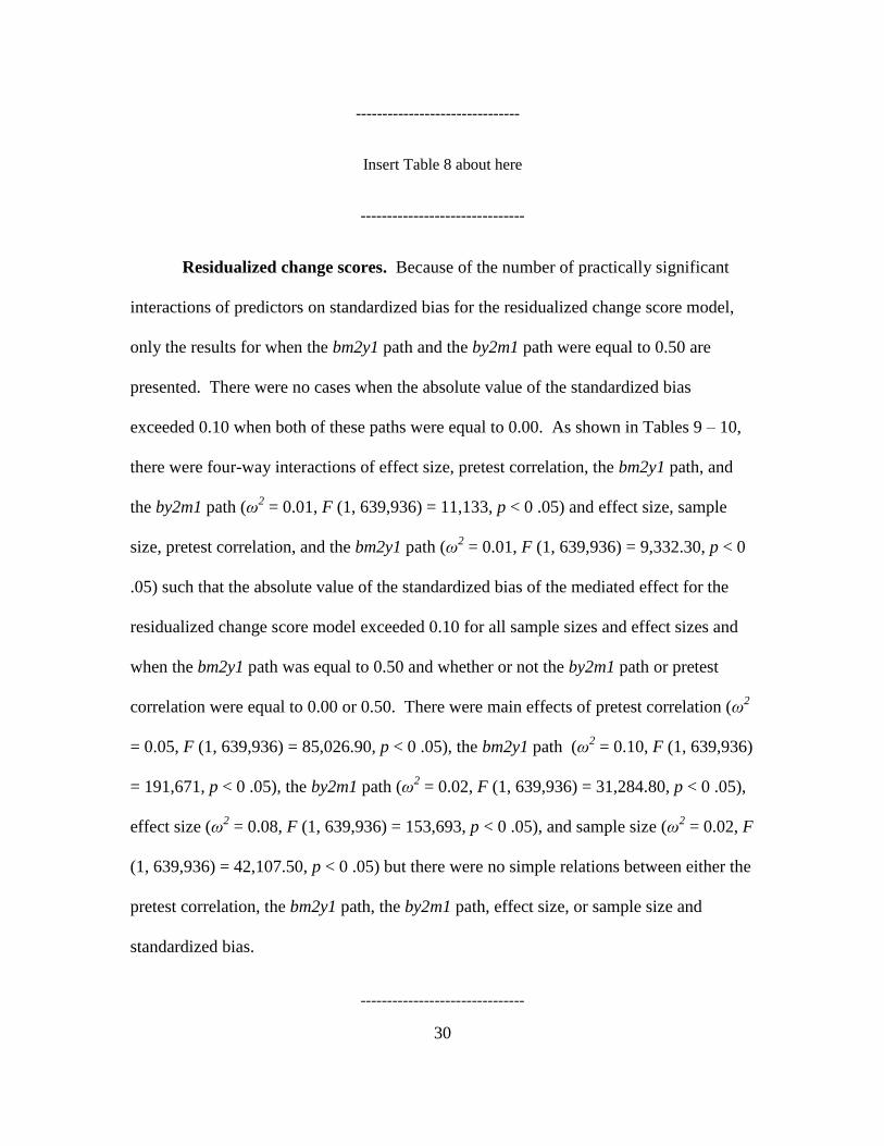
Residualized change scores. Because of the number of practically significant
interactions of predictors on standardized bias for the residualized change score model,
only the results for when the bm2y1 path and the by2m1 path were equal to 0.50 are
presented. There were no cases when the absolute value of the standardized bias
exceeded 0.10 when both of these paths were equal to 0.00. As shown in Tables 9 – 10,
there were four-way interactions of effect size, pretest correlation, the bm2y1 path, and
the by2m1 path (ω2 = 0.01, F (1, 639,936) = 11,133, p < 0 .05) and effect size, sample
size, pretest correlation, and the bm2y1 path (ω2 = 0.01, F (1, 639,936) = 9,332.30, p < 0
.05) such that the absolute value of the standardized bias of the mediated effect for the
residualized change score model exceeded 0.10 for all sample sizes and effect sizes and
when the bm2y1 path was equal to 0.50 and whether or not the by2m1 path or pretest
correlation were equal to 0.00 or 0.50. There were main effects of pretest correlation (ω2
= 0.05, F (1, 639,936) = 85,026.90, p < 0 .05), the bm2y1 path (ω2 = 0.10, F (1, 639,936)
= 191,671, p < 0 .05), the by2m1 path (ω2 = 0.02, F (1, 639,936) = 31,284.80, p < 0 .05),
effect size (ω2 = 0.08, F (1, 639,936) = 153,693, p < 0 .05), and sample size (ω
2 = 0.02, F
(1, 639,936) = 42,107.50, p < 0 .05) but there were no simple relations between either the
pretest correlation, the bm2y1 path, the by2m1 path, effect size, or sample size and
standardized bias.
-------------------------------

31
Insert Tables 9-10 about here
-------------------------------
Cross-Sectional.
Direct effect = 0.00. As shown in Table 11, the absolute value of the
standardized bias of the mediated effect with the cross-sectional model exceeded 0.10 for
all conditions and became larger when by2m1 increased from 0.00 to 0.50 and as sample
size increased (interaction of effect size, sample size, and the by2m1 path on the
standardized bias, ω2 = 0.01, F (1, 639,936) = 5,471.52, p < 0 .05). The standardized bias
was greater for effect sizes 0.01, 0.09, and 0.25 (ω2 = 0.16, F (1, 639,936) = 144,896, p <
0 .05), as sample size increased (ω2 = 0.03, F (1, 639,936) = 29,506.80, p < 0 .05), and as
the by2m1 path increased from 0.00 to 0.50 (ω2 = 0.03, F (1, 639,936) = 26,019.70, p < 0
.05).
------------------------------
Insert Table 11 about here
-------------------------------
Direct effect = 0.30. As shown in Tables 12 – 15 there was no interaction of
effect size, sample size, and the by2m1 path when the direct effect was present. There
were, however, interactions of effect size and sample size (ω2 = 0.01, F (1, 191,936) =
5,036, p < 0 .05), effect size and the by2m1 path (ω2 = 0.02, F (1, 191,936) = 7,067.87, p
< 0 .05), sample size and the by2m1 path (ω2 = 0.02, F (1, 191,936) = 7,193.63, p < 0
.05), pretest correlation and the bm2y1 path (ω2 = 0.01, F (1, 191,936) = 1,987.96, p < 0

32
.05), and the bm2y1 path and the by2m1 path (ω2 = 0.01, F (1, 191,936) = 3,990.23, p <
0 .05) such that the absolute value of the standardized bias exceeded 0.10 when the
bm2y1 path increased from 0.00 to 0.50 which increased when the pretest correlation
increased from 0.00 to 0.50, the by2m1 path increased from 0.00 to 0.50 and as effect size
and sample size increased. The standardized bias was the highest for N = 500 and large
effect sizes when the bm2y1 path was equal to 0.50, the by2m1 path was equal to 0.50,
and the pretest correlation was equal to 0.50. The only condition for which the absolute
value of the standardized bias did not exceed 0.10 was when the pretest correlation was
equal to 0.00, and both the bm2y1 path and the by2m1 path were equal to 0.00.
-------------------------------
Insert Tables 12 – 15 about here
-------------------------------
Relative Bias Results
ANCOVA. There were no main or interaction effects that were both statistically
significant and had omega-squared values of 0.01 or higher and there were no conditions
for which the relative bias exceeded 0.10.
Path Analysis. There were no main or interaction effects that were both
statistically significant and had omega-squared values of 0.01 or higher and there were no
conditions for which the relative bias exceeded 0.10.
33
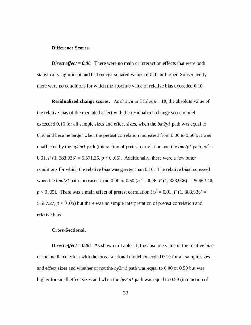
Difference Scores.
Direct effect = 0.00. There were no main or interaction effects that were both
statistically significant and had omega-squared values of 0.01 or higher. Subsequently,
there were no conditions for which the absolute value of relative bias exceeded 0.10.
Residualized change scores. As shown in Tables 9 – 10, the absolute value of
the relative bias of the mediated effect with the residualized change score model
exceeded 0.10 for all sample sizes and effect sizes, when the bm2y1 path was equal to
0.50 and became larger when the pretest correlation increased from 0.00 to 0.50 but was
unaffected by the by2m1 path (interaction of pretest correlation and the bm2y1 path, ω2 =
0.01, F (1, 383,936) = 5,571.36, p < 0 .05). Additionally, there were a few other
conditions for which the relative bias was greater than 0.10. The relative bias increased
when the bm2y1 path increased from 0.00 to 0.50 (ω2 = 0.06, F (1, 383,936) = 25,662.40,
p < 0 .05). There was a main effect of pretest correlation (ω2 = 0.01, F (1, 383,936) =
5,587.27, p < 0 .05) but there was no simple interpretation of pretest correlation and
relative bias.
Cross-Sectional.
Direct effect = 0.00. As shown in Table 11, the absolute value of the relative bias
of the mediated effect with the cross-sectional model exceeded 0.10 for all sample sizes
and effect sizes and whether or not the by2m1 path was equal to 0.00 or 0.50 but was
higher for small effect sizes and when the by2m1 path was equal to 0.50 (interaction of

34
effect size and the by2m1 path, ω2 = 0.01, F (1, 383,936) = 2,939.90, p < 0 .05). The
relative bias was larger when the pretest correlation increased from 0.00 to 0.50 (ω2 =
0.01, F (1, 383,936) = 2,443.24, p < 0 .05), when the by2m1 path increased from 0.00 to
0.50 (ω2 = 0.04, F (1, 383,936) = 17,133.80, p < 0 .05), and as effect size decreased (ω
2 =
0.02, F (1, 383,936) = 9,206.74, p < 0 .05).
Direct effect = 0.30. As shown in Tables 12 – 15, the same pattern of results
held for when there was a direct effect as compared to when there was not a direct effect.
The absolute value of relative bias of the mediated effect exceeded 0.10 for the cross-
sectional model when the by2m1 path increased from 0.00 to 0.50 and as effect size
decreased (interaction of effect size and by2m1 path, ω2 = 0.01, F (1, 191,936) = 3,265, p
< 0 .05). The relative bias increased as effect size decreased (ω2 = 0.05, F (1, 191,936) =
10,570.10, p < 0 .05), when the pretest correlation increased from 0.00 to 0.50 (ω2 = 0.01,
F (1, 191,936) = 1,342.46, p < 0 .05), when stability increased from 0.30 to 0.70 (ω2 =
0.01, F (1, 191,936) = 1,166.56, p < 0 .05), when the bm2y1 path increased from 0.00 to
0.50 (ω2 = 0.01, F (1, 191,936) = 1,138.91, p < 0 .05), and when the by2m1 path
increased from 0.00 to 0.50 (ω2 = 0.04, F (1, 191,936) = 9,089.92, p < 0 .05).
Summary.
In summary, the mediated effect was not biased when estimated with the
ANCOVA, path analysis, or difference score model. The mediated effect estimated with
the residualized change score model was biased when the pretest correlation was equal to
0.00 or 0.50 and the bm2y1 and by2m1 paths were equal to 0.50. When the bm2y1 and
by2m1 paths were equal to 0.00, the mediated effect was not biased and therefore

35
comparable to the mediated effect estimated with the ANCOVA and path analysis
models. The mediated effect was biased with the cross-sectional model when there was
no direct effect present (0.00) and became more biased as effect size increased and as the
by2m1 path increased from 0.00 to 0.50. When a direct effect was present, the only time
the mediated effect was not biased was when the pretest correlation was equal to 0.00 and
the by2m1 path was equal to 0.00. For this combination of conditions, the mediated
effect estimated with the cross-sectional model was comparable to the mediated effect
estimated with the ANCOVA and path analysis models.
Confidence Interval Coverage and Power Regression Analyses
Logistic regression analyses were conducted in the same way for confidence
interval coverage and power as for type 1 error rates with the addition of effect size of the
mediated effect as a standardized predictor in the analyses of confidence interval
coverage and power. For confidence interval coverage and power, separate analyses
were conducted for the conditions with no direct effect and for the conditions with a
direct effect because the direct effect manipulation was not completely crossed for all
levels of the other factors in this simulation study.
When assessing the performance of confidence interval coverage, coverage values
below 92.5% were considered low and were highlighted in red in the results tables.
Coverage values above 97.5% were considered high and were highlighted in green in the
results tables. These cutoff points correspond to Bradley’s (1978) robustness criterion.
The percent of cases falling above the upper limit and the percent of cases falling below
the lower limit did not differ across the models so those results were not reported here.

36
Confidence Interval Coverage.
ANCOVA. As shown in Table 16, the confidence interval coverage for the
ANCOVA model never fell below 92.5% for any combination of sample size and effect
size. There were a few instances when the coverage exceeded 97.5% which generally
happened when the effect was small (0.01) or zero and sample size was small (50 to 200).
There were no significant predictors of the confidence interval coverage of the mediated
effect with the ANCOVA model. That is, there were no significant main or interaction
effects that were both statistically significant and had a standardized beta coefficient with
an absolute value greater than 0.10.
-------------------------------
Insert Table 16 about here
-------------------------------
Path analysis. As shown in Table 17, the confidence interval coverage for the
path analysis model never fell below 92.5% for any combination of sample size and
effect size. There were a few instances when the coverage exceeded 97.5% which
generally happened when the effect size (0.01) and sample size was small (50 to 100).
There were no significant predictors of the confidence interval coverage of the mediated
effect with the path analysis model. That is, there were no significant main or interaction
effects that were both statistically significant and had a standardized beta coefficient with
an absolute value greater than 0.10.
-------------------------------

37
Insert Table 17 about here
-------------------------------
Difference scores. As shown in Table 18, the confidence interval coverage for
the path analysis model never fell below 92.5% for any combination of sample size and
effect size. There were a few instances when the coverage exceeded 97.5% which
generally happened when the effect size (0.01) and sample size was small (50 to 100).
There were no significant predictors of the confidence interval coverage of the mediated
effect with the path analysis model. That is, there were no significant main or interaction
effects that were both statistically significant and had a standardized beta coefficient with
an absolute value greater than 0.10.
-------------------------------
Insert Table 18 about here
-------------------------------
Residualized change scores.
Direct effect = 0.00. As shown in Tables 19 – 20 confidence interval coverage
fell below 92.5% as sample size, pretest correlation, and the bm2y1 path increased
(interaction of sample size, pretest correlation, and the bm2y1 path, b = -0.11, χ2 (1, N =
384,000) = 1,822.28, p < 0.05). Coverage was low for large sample sizes when the
pretest correlation the bm2y1 path both increased from 0.00 to 0.50. There was also an
interaction of pretest correlation, the bm2y1 path, and the by2m1 path (b = -0.11, χ2 (1, N
= 384,000) = 2,043.63, p < 0.05) such that as pretest correlation, the bm2y1 path, and the

38
by2m1 path all increased, coverage decreased. That is, coverage decreased when the
pretest correlation increased from 0.00 to 0.50 and when both the bm2y1 path and the
by2m1 path increased from 0.00 to 0.50. There were also main effects of the bm2y1 path
(b = -0.31, χ2 (1, N = 384,000) = 16,827.79, p < 0.05), sample size (b = -0.17, χ
2 (1, N =
384,000) = 4,303.29, p < 0.05), pretest correlation (b = -0.21, χ2 (1, N = 384,000) =
8,020.70, p < 0.05), and effect size (b = -0.13, χ2 (1, N = 384,000) = 2,529.66, p < 0.05)
but there were no simple interpretation of either the bm2y1 path, sample size, or effect
size and coverage.
The confidence interval coverage fell below 92.5% for the residualized change
score model for N = 50, when the effect size was 0.15 and 0.25 and when the bm2y1 path
was equal to 0.50 but the by2m1 path and the pretest correlation were equal to 0.00. The
confidence interval coverage was also low for N = 50, effect sizes 0.05, 0.09, 0.15, and
0.25 when the bm2y1 path and the pretest correlation were equal to 0.50 but the by2m1
path was equal to 0.00. When the by2m1 path increased from 0.00 to 0.50, the coverage
dropped to 92.5% for an additional effect size of 0.03. For N = 100, the confidence
interval coverage dropped below 92.5% for effect sizes 0.09, 0.15, and 0.25 when the
bm2y1 path, the by2m1 path, and the pretest correlation decreased from 0.50 to 0.00.
When the by2m1 path increased from 0.00 to 0.50, the coverage decreased for effect sizes
0.15 and 0.25. When the pretest correlation increased from 0.00 to 0.50, the coverage
decreased for effect sizes 0.03, 0.05, 0.09, 0.15, and 0.25 when the bm2y1 path increased
from 0.00 to 0.50 and whether or not the by2m1 path increased from 0.00 to 0.50.

39
For N = 200, the coverage was low for effect sizes 0.09, 0.15, and 0.25 when the
bm2y1 path increased from 0.00 to 0.50 but the by2m1 path and the pretest correlation
decreased from 0.50 to 0.00. When the by2m1 path increased from 0.00 to 0.50, the
coverage decreased for effect sizes 0.15 and 0.25. When the pretest correlation increased
from 0.00 to 0.50 the coverage decreased for effect sizes 0.03, 0.05, 0.09, 0.15, and 0.25
when the bm2y1 path increased from 0.00 to 0.50 but the by2m1 path decreased from
0.50 to 0.00. When the by2m1 path increased from 0.00 to 0.50, the coverage also
decreased for effect size 0.01 with the coverage decreasing to 0% in some cases. For N =
500, coverage was low for effect sizes, 0.03, 0.05, 0.09, 0.15, and 0.25 when the bm2y1
path was equal to 0.50, the pretest correlation was equal to 0.00 and whether or not the
by2m1 path increased was equal to 0.00 or 0.50. When the pretest correlation increased
from 0.00 to 0.50, coverage decreased for all effect sizes when the bm2y1 path increased
from 0.00 to 0.50 and whether or not the by2m1 path increased from 0.00 to 0.50. In
some cases, the coverage went to 0%. The confidence interval coverage exceeded 97.5%
for N = 50 and N = 100 when there was no effect or the effect size was small (0.01) and
occurred across both values of pretest correlation, the bm2y1 path, and the by2m1 path.
-------------------------------
Insert Tables 19-20 about here
-------------------------------

40
Direct effect = 0.30. As shown in Tables 21 – 22 there was an additional
interaction of sample size, pretest correlation and the by2m1 path (b = -0.10, χ2 (1, N =
192,000) = 416.01, p < 0.05) on the confidence interval coverage for the residualized
change score model when there was a direct effect present. As sample size, pretest
correlation, and the by2m1 path increased, the coverage decreased.
For N = 50 and effect size 0.25 the confidence interval coverage dropped below
92.5% when the bm2y1 path and the pretest correlation both increased from 0.00 to 0.50,
and when the by2m1 path decreased from 0.50 to 0.00. For N =100 and effect size 0.09
and 0.25, the confidence interval coverage dropped to or below 92.5% when the bm2y1
path increased from 0.00 to 0.50, and when the pretest correlation and the by2m1 path
both decreased from 0.50 to 0.00. It was also low for effect size 0.25 when the bm2y1
path and the pretest correlation both increased from 0.00 to 0.50 and when the by2m1
path decreased from 0.50 to 0.00. The coverage was also low for effect size 0.25 when
the bm2y1 path and the by2m1 path both increased from 0.00 to 0.50, and when the
pretest correlation decreased from 0.50 to 0.00. When the pretest correlation increased
from 0.00 to 0.50, the coverage decreased for effect sizes 0.01 and 0.25. A similar
pattern emerged for N = 200 and N = 500. The coverage exceeded 97.5% when the
by2m1 path increased from 0.00 to 0.50 and the bm2y1 path decreased from 0.50 to 0.00
for a range of effect sizes and exceeded 97.5% when the effect size was small (0.01).
-------------------------------
Insert Tables 21-22 about here
-------------------------------

41
Cross Sectional.
Direct effect = 0.00. As shown in Table 23, as sample size and effect size
increased, the confidence interval coverage of the cross-sectional model decreased
(interaction of sample size and effect size, b = -0.10, χ2 (1, N = 384,000) = 2,976, p <
0.05). The coverage decreased as a function of effect size more for large sample sizes
than small sample sizes. There was also an interaction of effect size and the by2m1 path
(b = -0.11, χ2 (1, N = 384,000) = 3,418.07, p < 0.05) such that as effect size and the
by2m1 path increased, coverage decreased. Coverage decreased as a function of effect
size more when the by2m1 path was equal to 0.50 than when the by2m1 path was equal
0.00 with coverage being as low as 0.02 in one case. The coverage was the lowest for
large effect sizes, large sample sizes, and when the by2m1 path was equal to 0.50. There
were also main effects of sample size (b = -0.23, χ2 (1, N = 384,000) = 16,296.86, p <
0.05), effect size (b = -0.23, χ2 (1, N = 384,000) = 16,855.86, p < 0.05), and the by2m1
path (b = -0.21, χ2 (1, N = 384,000) = 12,807.41, p < 0.05). In this case, there was no
simple relation between either sample size, effect size, or the by2m1 path and coverage.
For N = 50, confidence interval coverage fell below 92.5% for effect sizes 0.09,
0.15, and 0.25 when the by2m1 path increased from 0.00 to 0.50. For N = 100, coverage
decreased for effect size 0.25 when the by2m1 path decreased from 0.50 to 0.00 and for
effect sizes 0.09, 0.15, and 0.25 when the by2m1 path increased from 0.00 to 0.50. For N
= 200, coverage decreased for effect sizes 0.09, 0.15, and 0.25 when the by2m1 path
increased from 0.00 to 0.50 and decreased for effect sizes 0.01, 0.03, 0.09, 0.15, and 0.25
when the by2m1 path increased from 0.00 to 0.50. For N = 500, coverage decreased for

42
effect sizes 0.01, 0.09, 0.15, and 0.25 when the by2m1 path decreased from 0.50 to 0.00
and decreased for effect sizes 0.01 and higher when the by2m1 path increased from 0.00
to 0.50. Confidence interval coverage never exceeded 97.5%.
-------------------------------
Insert Table 23 about here
-------------------------------
Direct effect = 0.30. As shown in Table 24, there was an additional interaction of
sample size, effect size, and the by2m1 path (b = -0.12, χ2 (1, N = 192,000) = 2,243.01, p
< 0.05) on the confidence interval coverage of the cross-sectional model when there was
a direct effect present. That is, as sample size, effect size, and the by2m1 path increased,
the coverage decreased.
For N = 50 and N = 100 and effect sizes 0.09 and 0.25, the confidence interval
coverage dropped below 92.5% when the by2m1 path increased from 0.00 to 0.50. For N
= 200 and N=500 and effect sizes 0.01, 0.09, and 0.25, the coverage was low when the
by2m1 path increased from 0.00 to 0.50. There was a significant three-way interaction of
effect size, sample size, and by2m1 path (b = -0.12, χ2 (1, N = 192,000) = 2,243.01, p <
0.05) on the confidence interval coverage of the mediated effect for the cross-sectional
model. The confidence interval coverage never exceeded 97.5%.
-------------------------------
Insert Table 24 about here
-------------------------------

43
Summary.
In summary, the confidence interval coverage for the ANCOVA, path analysis,
and difference score model were similar and generally fell within the range of 92.5% -
97.5% coverage. The confidence interval coverage for the residualized change score
model was low when the pretest correlation and both the bm2y1 path and the by2m1 path
were equal to 0.50 and as sample size and effect size increased. The confidence interval
coverage for the residualized change score model was comparable to the confidence
interval coverage for the path analysis model when the bm2y1 path was equal to 0.00 and
whether or not the by2m1 or the pretest correlation was equal to 0.00 or 0.50. The results
for the confidence interval coverage for the cross-sectional model were low when the
by2m1 path was equal to 0.50 and as effect size and sample size increased. The
confidence interval coverage for the cross-sectional model was comparable to the
confidence interval coverage for the path analysis model when the by2m1 path was equal
to 0.00, when the sample size was small (N = 50), and when the effect size was less than
0.25.
Power Results
ANCOVA. As shown in Figure 2, as sample size and effect size increased
simultaneously, the power to detect the mediated effect increased substantially
(interaction of sample size and effect size, b = 0.25, χ2 (1, N = 384,000) = 9,748.88, p <
0.05). Power increased as a function of effect size faster for large sample sizes (N = 500)
compared to small sample sizes (N = 50). Power to detect the mediated effect using the
ANCOVA model increased as sample size (b = 0.36, χ2 (1, N = 384,000) = 27,071.26, p <

44
0.05) and effect size (b = 0.55, χ2 (1, N = 384,000) = 61,739.35, p < 0.05) increased.
Overall, power reached 0.80 or higher for N = 50 when the effect size was 0.25, for N =
100 when the effect size was 0.15 or higher, for N = 200 when the effect size was 0.09 or
higher, and for N = 500 when the effect size was 0.09 or higher.
- Insert Figure 2 about here –
Path analysis. As shown in Figure 3, as sample size and effect size increased
simultaneously, the power to detect the mediated effect increased substantially
(interaction of sample size and effect size, b = 0.24, χ2 (1, N = 384,000) = 8,738.57, p <
0.05). Power increased as a function of effect size faster for large sample sizes (N = 500)
compared to small sample sizes (N = 50). Power to detect the mediated effect using the
path analysis model increased as sample size (b = 0.35, χ2 (1, N = 384,000) = 25,179.87,
p < 0.05) and effect size (b = 0.56, χ2 (1, N = 384,000) = 61,661.44, p <0.05) increased.
Overall, power reached 0.80 or higher for N = 50 when the effect size was 0.25, for N =
100 when the effect size was 0.15 or higher, for N = 200 when the effect size was 0.09 or
higher, and for N = 500 when the effect size was 0.09 or higher.
- Insert Figure 3 about here –
Difference scores. As shown in Figure 4, as sample size, effect size, and stability
increased simultaneously, the power to detect the mediated effect increased substantially
(interaction of sample size, effect size, and stability, b = 0.12, χ2 (1, N = 384,000) =
3,220.13, p < 0.05). Power increased as sample size and effect size increased but power
increased faster when stability was equal to 0.70 compared to when stability was equal to
0.30. Power to detect the mediated effect with the difference score model increased as

45
sample size increased (b = 0.31, χ2 (1, N = 384,000) = 31,624.90, p < 0.05), effect size
increased (b = 0.41, χ2 (1, N = 384,000) = 46,292.63, p < 0.05), and stability increased (b
= 0.19, χ2 (1, N = 384,000) = 17,024.69, p < 0.05). Overall, power reached 0.80 or higher
for N = 50 and stability = 0.70 when the effect size was 0.25, for N = 100 and stability =
0.70 when the effect size was 0.15 or higher, for N = 200 and stability = 0.70 for effect
sizes 0.09 or higher, and for N = 500 and stability = 0.70 for effect sizes 0.09 or higher.
Power never reached 0.80 when stability was equal to 0.30 for any combination of effect
size and sample size.
- Insert Figure 4 about here –
Residualized change scores.
Direct effect = 0.00. A caveat should be mentioned. Because the residualized
change score model resulted in biased estimates of the mediated effect, power results
should be interpreted with caution. As shown in Figure 5, as sample size and effect size
increased simultaneously the power to detect the mediated effect with the residualized
change score model increased substantially (interaction of sample size and effect size, b =
0.29, χ2 (1, N = 384,000) = 17,289.46, p < 0.05). Power increased as effect size increased
but power increased faster for large sample sizes (N = 500) than small sample sizes (N =
50). Power to detect the mediated effect with the residualized change score model
increased as sample size increased (b = 0.36, χ2 (1, N = 384,000) = 38724.90, p < 0.05)

46
and effect size increased (b = 0.47, χ2 (1, N = 384,000) = 58207.76, p < 0.05). Power
decreased when the bm2y1 path increased from 0.00 to 0.50 (b = -0.11, χ2 (1, N =
384,000) = 1901.00, p < 0.05).
Overall, power reached 0.80 or higher for N = 50 and bm2y1 path equal to 0.00
for effect size 0.25, for N = 100 and bm2y1 path equal to 0.00 for effect size 0.15 or
higher, for N = 200 and bm2y1 path equal to 0.00 for effect size 0.09 or higher, for N =
500 and bm2y1 path equal to 0.00 for effect size 0.09 or higher. Power also reached 0.80
or higher when the bm2y1 path was equal to 0.50 for N = 200 and N = 500 and for effect
sizes 0.15 or higher.
- Insert Figure 5 about here -
Direct effect = 0.30. As shown in Figure 6 and Figure 7, power decreased when
either the by2m1 or bm2y1 paths increased from 0.00 to 0.50 for small sample sizes more
than large sample sizes (interaction of sample size and by2m1 path, b = -0.10, χ2 (1, N =
192,000) = 705.35, p < 0.05, and interaction of sample size and the bm2y1 path, b = -
0.10, χ2 (1, N = 192,000) = 739.36, p < 0.05). The decrease in power was more
pronounced for N = 50, 100, and 200 but power was still low for N = 500 when either or
both the by2m1 path and bm2y1 path increased from 0.00 to 0.50.
Power increased less as effect size increased when either the by2m1 path or the
bm2y1 path was equal to 0.50 than when either by2m1 path or the bm2y1 path was equal
to 0.00 (interactions of effect size and by2m1 path, b = -0.10, χ2 (1, N = 192,000) =
1,068.48, p < 0.05) and effect size and bm2y1 path, b = -0.10, χ2 (1, N = 192,000) =
1,047.38, p < 0.05). In general, power decreased when either the by2m1 path was equal

47
to 0.50 (b = -0.13, χ2 (1, N = 192,000) = 1,828.92, p < 0.05) or the bm2y1 path was equal
to 0.50 (b = -0.13, χ2 (1, N = 192,000) = 1,976.48, p < 0.05).
Overall, power reached 0.80 or higher for N = 50 when the bm2y1 path and the
by2m1 path were equal to 0.00 for effect size 0.25, for N = 100 when either the bm2y1
path or the by2m1 path were equal to 0.50 for effect size 0.25, for N = 200 when either
the bm2y1 path or the by2m1 path was equal to 0.50 for effect size 0.09 or higher, for N =
500 when either the bm2y1 path or the by2m1 path was equal to 0.50 for effect size 0.09.
The only case when power reached 0.80 or higher and when both the bm2y1 path and the
by2m1 path were equal to 0.50 was for N = 500 and for effect size 0.25.
- Insert Figures 6 - 7 about here -
Cross-sectional.
Direct effect = 0.00. Because the cross-sectional model resulted in biased
estimates of the mediated effect, power results should be interpreted with caution. As
shown in Figure 8, as sample size and effect size increased simultaneously, the power to
detect the mediated increased substantially (interaction of sample size and effect size, b =
0.24, χ2 (1, N = 384,000) = 10,063.63, p < 0.05). Power increased as effect size increased
faster for large sample sizes than small sample sizes. Power to detect the mediated effect
with the cross-sectional model increased as sample size increased (b = 0.32, χ2 (1, N =
384,000) = 28,117.66, p < 0.05) and effect size increased (b = 0.51, χ2 (1, N = 384,000) =
62,557.86, p < 0.05). Overall, power reached 0.80 or higher for N = 50 when the effect
size was 0.25, for N = 100 when the effect size was 0.25, for N = 200 when the effect
size was 0.09 or higher, and for N = 500 when effect size was 0.09 or higher.

48
- Insert Figure 8 about here -
Direct effect = 0.30. As shown in Figure 9, power decreased as stability
increased from 0.30 to 0.70 more for small sample sizes than large sample sizes
(interaction of sample size and stability, b = -0.10, χ2 (1, N = 192,000) = 553.42, p <
0.05) and power decreased as stability increased from 0.30 to 0.70 more for small effect
sizes than large effect sizes (interaction of effect size and stability, b = -0.10, χ2 (1, N =
192,000) = 897.22, p < 0.05). Power decreased as stability increased from 0.30 to 0.70 (b
= -0.11, χ2 (1, N = 192,000) = 1,108.92, p < 0.05). Overall, power reached 0.80 or higher
for N = 50 and stability equal to 0.30 for effect size 0.25, for N = 100 when effect size
was 0.25 regardless of stability (0.30 vs. 0.70), for N = 200 when effect size was 0.09 and
higher regardless of stability (0.30 vs. 0.70), and for N = 500 for effect size 0.09 or higher
regardless of stability (0.30 vs. 0.70).
- Insert Figure 9 about here -
Summary.
In summary, the power results for the ANCOVA, path analysis, and difference
score models were similar for direct effect equal to 0.00 and direct effect equal to 0.30
conditions. It was expected the ANCOVA and path analysis model results would be
similar because they are identical models with the exception that ANCOVA uses ordinary
least squares (OLS) to estimate model parameters whereas path analysis uses maximum
likelihood (ML) to estimate model parameters.

49
All models achieved power of 0.80 or higher for some combinations of effect size
of the mediated effect and sample size. The ANCOVA and path analysis models
achieved power of 0.80 or higher with the lowest combination of effect size for the
mediated effect and sample size. The difference score model readily achieved power of
0.80 or higher as long as stability was equal to 0.70. The difference score model did not
achieve power of 0.80 or higher for any combination of effect size and sample size when
stability was equal to 0.30. The residualized change score model achieved power of 0.80
or higher unless both the bm2y1 path and the by2m1 path were equal to 0.50. When the
bm2y1 path and the by2m1 path were equal to 0.50, the residualized change score model
did not achieve power of 0.80 or higher regardless of effect size or sample size. The
cross-sectional model performed similarly to the ANCOVA and path analysis models.
ANCOVA vs. Cross-sectional. Because the cross-sectional model resulted in
biased estimates of the mediated effect, power results should be interpreted with caution.
When comparing the significance across models for some power analyses (e.g.,
ANCOVA vs. cross-sectional), the dependent variable was created by taking the absolute
value of the difference in conclusions each model reached regarding statistical
significance of the mediated effect. For example, for each model, the dependent variable
was ‘0’ for ‘non-significant mediated effect’ and ‘1’ for ‘significant mediated effect.
When comparing the performance of one model to another (e.g., ANCOVA vs. cross-
sectional) the absolute value of the difference of this value (0 or 1) for each model was
taken as the dependent variable to use for model comparisons of statistical significance of
the mediated effect. The coding scheme resulted in a variable that was coded ‘1’ if, for
that particular observation, there was a difference in the statistical conclusion regarding

50
the significance of the mediated effect across the two models and coded ‘0’ if, for that
particular observation, there was no difference in the statistical conclusion regarding the
significance of the mediated effect. The same procedure was followed for all
comparisons across models. These new variables were analyzed with logistic regression
analyses previously described in the type 1 error rates section.
As shown in Figure 10, there was an interaction of sample size and effect size on
the differences in power across the ANCOVA and cross-sectional model (b = -0.19, χ2 (1,
N = 384,000) = 10,497.68, p < 0.05). The cross-sectional model had more power than the
ANCOVA model for effect size of 0.01 for N = 50 to 500 and for effect sizes 0.03 and
0.05 for N = 50. The ANCOVA model had more power than the cross-sectional model
across all other combinations of sample size and effect size. There were also main effects
of sample size (b = -0.11, χ2 (1, N = 384,000) = 4,357.81, p < 0.05) and effect size (b = -
0.14, χ2 (1, N = 384,000) = 7,308.63, p < 0.05) but these main effects were not interpreted
because there was no simple relation between either sample size or effect size and
differences in power across the two models.
- Insert Figure 10 about here -
Path Analysis vs. Cross-sectional. As shown in Figure 11, the cross-sectional
model had more power than the path analysis model for effect size of 0.01 for N = 50 to
500 and for effect sizes 0.03 for N = 50 (interaction of sample size and effect size, b = -
0.19, χ2 (1, N = 384,000) = 10,481.10, p < 0.05). The path analysis model had more
power than the cross-sectional model across all combinations of sample size and effect
size. There were also main effects of sample size (b = -0.11, χ2 (1, N = 384,000) =

51
4,461.01, p < 0.05) and effect size (b = -0.14, χ2 (1, N = 384,000) = 7,442.22, p < 0.05)
but there was no simple relation between either sample size or effect size and the
differences in power across the two models.
- Insert Figure 11 about here -
Difference Scores vs. Cross-sectional.
Direct effect = 0.00. As shown in Figure 12 and Figure 13, there was an
interaction of effect size, stability, and by2m1 path (b = 0.10, χ2 (1, N = 384,000) =
3,099.08, p < 0.05) such that the cross-sectional model had more power than the
difference score model for all effect sizes and values of the by2m1 path when the stability
was 0.30. When stability increased to 0.70, the power for the cross-sectional model and
difference score model became more similar except for a discrepancy at effect size 0.15
and 0.25 for N =50, when the by2m1 path was equal to 0.00, and for effect size 0.15 for N
= 100.
As sample size (b = -0.10, χ2 (1, N = 384,000) = 2,709.765, p < 0.05) and stability
(b = -0.13, χ2 (1, N = 384,000) = 6,778.41, p < 0.05) increased, the differences in power
across the difference score model and the cross-sectional model became less pronounced.
Overall, the differences in power between the two models was affected less by the
inclusion of the by2m1 path and became less discrepant as sample size and stability
increased.
- Insert Figures 12 - 13 about here -

52
Direct effect = 0.30. As shown in Figure 14, when the direct effect was present
there was no longer an interaction of effect size, stability and the by2m1 path. Power
across the difference score model and the cross-sectional model did become less
discrepant for medium to large effect sizes as sample size increased (interaction of
sample size and effect size, b = -0.23, χ2 (1, N = 192,000) = 5,551.16, p < 0.05). The
difference in power across these models was almost zero for a small effect size (0.01).
The cross-sectional model had more power than the difference score model for all
effect sizes when stability was 0.30 but as stability increased to 0.70, the power for the
cross-sectional model and difference score model was almost identical (interaction of
effect size and stability, b = -0.13, χ2 (1, N = 192,000) = 2,308.15, p < 0.05). In this case,
the difference score model had more power than the cross-sectional model for effect size
0.25 for N = 50. Overall, the difference in power between the difference score model and
the cross-sectional model became less discrepant for medium to large effect sizes as
sample size and stability increased.
- Insert Figure 14 about here -
Residualized Change scores vs. Cross-sectional. As shown in Figure 15, the
residualized change score model had more power than the cross-sectional model for
effect sizes 0.10 and 0.15 for N = 100, effect sizes 0.03, 0.05, and 0.15 for N = 200, and
for effect sizes 0.03 and 0.05 for N = 500 (interaction of sample size and effect size, b =
0.22, χ2 (1, N = 384,000) = 11,984.99, p < 0.05). The cross-sectional model had more
power than the residualized change score model for all other combinations of sample size
and effect size. There were also main effects of sample size (b = -0.13, χ2 (1, N =

53
384,000) = 5,150.72, p < 0.05) and effect size (b = -0.11, χ2 (1, N = 384,000) = 4,330.22,
p < 0.05) but there was no simple relation between either sample size or effect size and
the differences in power across the two models.
- Insert Figure 15 about here –
Path analysis vs. Difference score.
Because the path analysis model and the ANCOVA model are identical models,
only comparisons between the path analysis model and the difference score model and
the residualized change score model were presented. The path analysis model was
treated as the “ideal” model to use as a benchmark for the other models because it
estimates all the parameters of the covariance structure in the pretest – posttest control
group design with a mediating variable.
Direct effect = 0.00. As shown in Figures 16 – 17, there was more discrepancy in
the power across the path analysis and difference score models when sample sizes were
small and stability was equal to 0.30 (interaction of sample size and stability, b = -0.10, χ2
(1, N = 384,000) = 1,069.97, p < 0.05), more discrepancy in the power results for medium
to large effect sizes for small sample sizes (interaction of sample size and effect size, b =
-0.24, χ2 (1, N = 384,000) = 5,326.53, p < 0.05), and more discrepancy in the power
results for medium to large effect sizes when the stability was equal to 0.30 (interaction
of effect size and stability, b = -0.15, χ2 (1, N = 384,000) = 2,857.50, p < 0.05).
The discrepancy between the models decreased as both sample size (b = -0.14, χ2
(1, N = 384,000) = 1,935.26, p < 0.05) and stability increased (b = -0.22, χ2 (1, N =

54
384,000) = 7,394.77, p < 0.05). The discrepancy between the model became more
extreme when the by2m1 path increased from 0.00 to 0.50 (b = 0.10, χ2 (1, N = 384,000)
= 1,539.44, p < 0.05). Overall, there is a large discrepancy in power across the path
analysis and difference score model for N = 50 – 100, when stability was equal to 0.30
and when the by2m1 path was equal to 0.50 for effect size 0.09 and higher. The
discrepancy between the models became less extreme as stability increased to 0.70 and
there was less discrepancy for N = 200 – 500 regardless of the value of the by2m1 path
and effect size.
- Insert Figures 16 – 17 about here –
Direct effect = 0.30. As shown in Figures 18 – 21, when the direct effect was
present, there was no longer an interaction between sample size and stability. All effects
that were present when the direct effect equaled 0.00 were present with the addition of an
interaction of the bm2y1 path and the by2m1 path (b = -0.10, χ2 (1, N = 192,000) =
406.04, p < 0.05) such that the discrepancy between the models was more pronounced
when the bm2y1 path was equal to 0.50 and the by2m1 path was equal to 0.50. There was
an interaction of effect size and the by2m1 path (b = 0.10, χ2 (1, N = 192,000) = 493.51, p
< 0.05) such that the discrepancy was more pronounced for medium to large effect sizes
when the by2m1 path was equal to 0.50. There was a main effect of the by2m1 path (b =
0.13, χ2 (1, N = 192,000) = 690.86, p < 0.05) but there was not a simple relation between
the by2m1 path and the differences in power across the two models. Overall, there was a
large discrepancy in power across the path analysis model and the difference score model
when stability was equal to 0.30 and either the bm2y1 path or the by2m1 path were equal

55
to 0.50. As stability increased to 0.70, the discrepancy between the models virtually
disappeared for all combinations of effect size, sample size, and values of the bm2y1 path
and the by2m1 path.
- Insert Figures 18 – 21 about here –
Path analysis vs Residualized change score. Because the residualized change
score model resulted in biased estimates of the mediated effect, power results should be
interpreted with caution. As shown in Figures 22 – 23, the discrepancy between the path
analysis model and the residualized change score model was more pronounced for
medium to large effect sizes for small sample sizes than large sample sizes (interaction of
sample size and effect size, b = -0.24, χ2 (1, N = 384,000) = 3,513.36, p < 0.05). The
discrepancy between the models became less pronounced as sample size increased (b = -
0.19, χ2 (1, N = 384,000) = 2,417.01, p < 0.05), as effect size increased (b = -0.12, χ
2 (1,
N = 384,000) = 1,095.76, p < 0.05), when the bm2y1 path decreased from 0.50 to 0.00 (b
= 0.20, χ2 (1, N = 384,000) = 3761.27, p < 0.05) and when the by2m1 path decreased
from 0.50 to 0.00 (b = 0.09, χ2 (1, N = 384,000) = 813.10, p < 0.05). Overall, there was a
large discrepancy in power across the path analysis model and the residualized change
score model when either the bm2y1 path or the by2m1 path were equal to 0.50 for
medium to large effect sizes for N = 50 to 100. When the sample size increased to N =
200 and higher, there was only a discrepancy between the models when both the bm2y1
path and the by2m1 path were equal to 0.50 for medium to large effect sizes.
- Insert Figures 22 – 23 about here –
Summary.

56
In summary, the power results across the ANCOVA and path analysis models
compared to the cross-sectional model were generally not discrepant except when the
effect size of the mediated effect was small (0.01). The power results across the
difference score model compared to the cross-sectional model were discrepant when
stability was equal to 0.30 and the by2m1 path was equal to 0.50. Any discrepancies
between these two models went away when stability increased to 0.70 and sample size
increased. The power results across the residualized change score model compared to the
cross-sectional model were discrepant for numerous values of effect size of the mediated
effect and across all sample sizes. Despite the discrepancy for numerous conditions, the
two models had similar power curves across all combinations of sample size and effect
size.
The power results across the path analysis model compared to the difference score
model were discrepant when stability was equal to 0.30 and either the bm2y1 path or the
by2m1 path was equal to 0.50. Any discrepancies between these models generally went
away as stability increased to 0.70 and sample size increased regardless of the value of
the bm2y1 path or the by2m1 path. The power results across the path analysis model
compared to the residualized change score model were discrepant when the bm2y1 path
or the by2m1 path was equal to 0.50. The discrepancies between these models went away
as sample size increased and as either the bm2y1 or the by2m1 path decreased to 0.00.
Ancillary Analyses
A comparison was made between the sample size needed to detect the mediated
effect of a given effect size to achieve power of 0.80 or greater from this simulation study

57
and the sample size needed to detect a mediated effect to achieve power of 0.80 from
Fritz and MacKinnon (2007). As shown in Table 25, there was a general consensus with
the sample size and effect size combination that was needed to detect the mediated effect
with power of 0.80 or higher in this simulation study compared to the sample size and
effect size combination that was needed to detect a mediated effect with 0.80 power from
Fritz and MacKinnon (2007). One discrepancy occurs when the effect size of the
mediated effect was small (0.02 – 0.03). In this simulation study, when the effect size
was small (0.03) and sample size was equal to 500, the power to detect a significant
mediated effect with the cross-sectional model was 0.46. Fritz and MacKinnon (2007)
demonstrated that when the effect size of the mediated effect was small (0.02) a sample
size of 533 was required to detect a significant mediated effect. Therefore, the cross-
sectional estimate of the mediated effect is under-powered for small effect sizes when the
underlying model is a longitudinal mediation model.
A summary index was created that represented the percentage of times a mediated
effect was detected for each of the five models as a way to gauge the consensus regarding
the significance of the mediated effect across all five models. This index was created as a
five digit number with each digit representing one of the five models’ decision of
detecting a significant mediated effect (i.e., labeled ‘1’) or not detecting a significant
mediated effect (i.e., labeled ‘0’). The first digit in this index represented the path
analysis model, the second represented the ANCOVA model, the third represented the
residualized change score model, the fourth represented the difference score model, and
the fifth represented the cross-sectional model. For example, the first row of Table 26 is
the five digit number ‘00000’ with percent equal to 36.18% which indicates that all five

58
models reached the same conclusion of not detecting the mediated effect 36.18% of time.
The second row is the five digit number ‘00001’ with percent of occurrence of 3.79%
which indicates that less than 4% of the time the only model that indicated a significant
mediated effect was the cross-sectional model.
-------------------------------
Insert Table 25 about here
-------------------------------
For all models, the same conclusion of not detecting a mediated effect (36.18%)
and the same conclusion of detecting the mediated effect (29.29%) was observed. The
difference score model was the only model that did not detect the mediated effect 10.84%
of the time. The residualized change score model was the only model that did not detect
the mediated effect 4.14% of the time. The cross-sectional model was the only model
that did not detect the mediated effect 3.81% of the time and it was the only model to
detect the mediated effect 3.79% of the time. Further, 3.47% of the time the residualized
change score and difference score models did not detect the mediated effect while the
other models did. Lastly, 1.09% of the time the cross-sectional and difference score
models did not detect the mediated effect while the other models did and 1.17% of the
time the cross-sectional and residualized change score models did not detect the mediated
effect while the other models did. Overall, there is a high percentage of occurrence of all
models reaching the same conclusion (65.47%) regarding detecting either a significant
mediated effect or a non-significant mediated effect.

59
-------------------------------
Insert Table 26 about here
-------------------------------
A two-dimensional plot was created using tetrachoric correlations between the
power of each of the five models. The dimension on the y-axis represents whether or not
the models estimated the stability of the mediator and outcome variables across time and
how they estimated the stability and the dimension on the x-axis represents how the
models that did not measure the stability were differentially affected by the stability. The
ANCOVA, path analysis, and residualized change score models all estimated the stability
of the mediator and outcome variables but they did so differently therefore they are
clustered close together and separated from the cross-sectional and difference score
models. The cross-sectional and difference score models were affected differently by
stability because neither the cross-sectional nor difference score model estimated the
stability and they each made different assumptions regarding the stability. For example,
the difference score model assumes that the stability is equal to 1.0 and we can think of
the cross-sectional model as assuming the stability is equal to 0.0 which explains why
each of these models are opposite each other on the dimension ‘Effect of stability’.
- Insert Figure 24 about here –
Summary
Overall, the best performing models were the ANCOVA and the path analysis
model in terms of type 1 error, bias, confidence interval coverage, and power. The

60
difference score model performed well in terms of type 1 error, bias, confidence interval
coverage, and power but it never outperformed the ANCOVA or path analysis models.
The performance of the residualized change score and cross-sectional models were
negatively affected when the pretest correlation was non-zero between the mediator and
the outcome and when there were non-zero cross-lagged paths (by2m1 and bm2y1).
When the pretest correlation was zero and the cross-lagged paths were zero, the
performance of the residualized change score and cross-sectional models were
comparable to the ANCOVA and path analysis models in this simulation but these
models (residualized change score and cross-sectional) did not consistently outperform
the ANCOVA and path analysis models.
Discussion
The aim of this project was to compare four common longitudinal models and the
cross-sectional model for assessing the mediated effect in the pretest – posttest control
group design. The main conclusion of this project is that the only models that were not
biased, did not have inflated Type 1 error rates, and had high empirical power were the
ANCOVA and path analysis models. Recall the effect size of the mediated effect in this
project was the product of the effect size of the coefficient relating the treatment to the
mediator at posttest and the coefficient relating the mediator at posttest to the outcome at
posttest adjusting for all other effects in the model. The effect sizes for each of the
coefficients were picked to reflect small, medium, and large effects in the correlation
metric with the effect size of the mediated effect being the product of these effect sizes.
When the sample size was small (N = 50), the ANCOVA and path analysis models
reached 0.80 or higher when the effect size of the mediated effect was 0.25 (which

61
corresponds to a large effect for both the am2x and by2m2 paths). When the sample size
was slightly larger (N = 100), the ANCOVA and path analysis models reached 0.80 when
the effect size of the mediated effect was 0.15 (which corresponds to a medium and large
effect size for either the am2x or by2m2 path). Finally, when the sample size was large
(N = 200 to N = 500), the ANCOVA and path analysis models reached 0.80 power when
the effect size of the mediated effect was 0.09 (which corresponds to medium effects for
both the am2x and by2m2 paths) or higher.
The ANCOVA and path analysis models performed the best because they
estimated every parameter of the covariance structure for mediation in the pretest –
posttest control group design. That is, these models took into account the pretest
correlation between the mediator and the outcome, the stability of the mediator and the
outcome, and any cross-lagged relations between the pretest measures and the posttest
measures. Further, the ANCOVA and path analysis models performed the best because
they most closely matched the data-generating model of this simulation study.
Researchers should use either the ANCOVA or path analysis models when assessing the
mediated effect in the pretest – posttest control group design.
The difference score, residualized change score, and the cross-sectional model all
produced biased estimates of the mediated effect or had low empirical power for some
conditions of this simulation study. The difference score model was generally not biased
even when there was a pretest correlation and cross-lagged relations. Despite not
producing a biased estimate of the mediated effect, the difference score model did not
have as high empirical power as did the ANCOVA/path analysis model and the empirical

62
power of the difference score model decreased as stability of the mediator and outcome
decreased. The residualized change score model and the cross-sectional model produced
biased estimates of the mediated effect when either of the cross-lagged paths were
present. The estimate of the mediated effect also became more biased when there was a
pretest correlation compared to when the pretest correlation was not present for the
residualized change and cross-sectional model. However, when the cross-lagged paths
and the pretest correlation was zero in the population model, the residualized change
score and cross-sectional models did not produce biased estimates of the mediated effect.
The residualized change score model had comparable power to the ANCOVA/path
analysis model when the pretest correlation and cross-lagged paths were zero. The cross-
sectional model had lower power than the ANCOVA/path analysis model except in a few
instances when the sample size was small and the effect size of the mediated effect was
small. The empirical power to detect the mediated effect with the cross-sectional model
decreased as stability of the mediator and outcome increased.
Because the difference score model did not produce a biased estimate of the
mediated effect and because type 1 error rates were not above the nominal 0.05 alpha
level, a researcher could estimate the mediated effect with the difference score model and
have empirical power similar to the ANCOVA or path analysis models as long as the
stability of the mediator and outcome is high. The residualized change score model
requires that more conditions are met in order for unbiased estimation of the mediated
effect and empirical power similar to the ANCOVA and path analysis models. If there is
no pretest correlation and no cross-lagged relations, a researcher could estimate the
mediated effect with the residualized change score model and produce an unbiased

63
estimate of the mediated effect with comparable albeit lower power than the
ANCOVA/path analysis model. In order for the cross-sectional model to unbiasedly
estimate the mediated effect in the pretest – posttest control group design, similar
conditions are needed. The mediated effect will not be biased using the cross-sectional
model when there are no cross-lagged paths and when there is no pretest correlation
between the mediator and the outcome. Additionally, the power to detect the mediated
effect with the cross-sectional model will be comparable to the power to detect the
mediated effect using the ANCOVA/path analysis model if the pretest correlation and
cross-lags are zero and if stability of the mediator and outcome is low. Given a pretest –
posttest control group design with low stability of the mediator and outcome, no pretest
correlation, and no cross-lagged relations, a researcher could estimate the mediated effect
with the cross-sectional model and have empirical power comparable to the ANCOVA or
path analysis models and have an unbiased estimate of the mediated effect.
Although there exist conditions for which a researcher could estimate the
mediated effect for all the models mentioned, it is not recommended for researchers to
use the difference score, residualized change score, or cross-sectional models when
estimating mediated effects in the pretest – posttest control group design because there
were no conditions for which these models outperform the ANCOVA/path analysis
model. Also, it may be difficult to find evidence of these conditions in sample data
(especially with small samples) so either the ANCOVA or the path analysis model would
be the best model for this research design.

64
The results provide practical insight about the conditions needed when using the
cross-sectional, difference score, and residualized change score models. That is, when
researchers use the cross-sectional, difference score, or residualized change score model
to estimate mediated effects in the pretest – posttest control group design, there are
additional conditions that need to be met regarding the relation between the pretest
measures of the mediator and outcome variable and conditions that need to be met
regarding the relations between the pretest measures and the posttest measures of the
mediator and outcome variables. These additional conditions may be untenable but if
they are satisfied, then the estimation of mediated effects can be unbiased and have
empirical power similar to the ANCOVA or path analysis models.
Implications
Researchers can apply several different models when assessing mediated effects
in the pretest – posttest control group design including the cross-sectional model, the
difference score model, the residualized change score model, ANCOVA, and path
analysis. Given the findings of this study, anytime researchers use the cross-sectional
model (Jouriles et al., 2010), the difference score model (Hofmann, 2004; Jansen et al.,
2012; MacKinnon et al., 1991), or the residualized change score model (Cole, et al.,
2003; Miller, et al., 2002; Reid & Aiken, 2013) they are making assumptions about the
conditions that need to be met regarding the relations between the pretest variables and
any cross-lagged relations across time. In general, the assumption is there are no
relations between the pretest variables or cross-lagged relations. When these conditions
are met the cross-sectional model and residualized change score model result in biased

65
mediated effect estimates and low empirical power to detect the mediated effect even
when these conditions are met. The difference score model never resulted in biased
estimates of the mediated effect but it did have low empirical power in some case. If
researchers use the cross-sectional, change score, or residualized change score model,
they may be inadvertently missing true mediated effects that are present and they may be
reporting biased estimates of true mediated effects.
Previous research has expounded on the limitations of using cross-sectional data
to estimate mediated effects (Gollob & Reichardt, 1991; Maxwell & Cole, 2007;
Maxwell, Cole, & Mitchell, 2011). Cross-sectional estimates of mediated effects will
often be biased because they do not allow for mediating variables (M) to exert their
influence on outcome variables (Y), which presumably occurs over a specific period of
time. As time interval varies, so do estimates of mediated effects because estimates of
mediated effects depend on the time interval during which they are assessed. This study
confirms the general findings of previous literature regarding the bias of the cross-
sectional mediated effect as an estimate of a longitudinal mediated effect. The
implications of the findings of this study is that there are some conditions for which the
cross-sectional estimate of the mediated effect is unbiased (i.e., when there is no pretest
correlation or cross-lagged relations) and that there were no cases for which the cross-
sectional model ever resulted in type 1 error rates above the nominal 0.05 alpha level.
These implications build on previous research and provide a more detailed picture of
when the cross-sectional model will result in biased estimates of longitudinal mediated
effects and how this affects empirical power and type 1 error rates.

66
Limitations
This project compared longitudinal models and the cross-sectional model in the
pretest – posttest control group design. Recall, the pretest – posttest control group design
involves the random assignment of units to either a treatment or a control group.
Successful randomization of units to groups in this experimental design ensures that any
pre-existing differences between the units in the treatment and control groups are due to
chance and do not reflect systematic differences. Therefore, the results of this project do
not necessarily extend to situations for which there are systematic pre-existing
differences between the units in groups that are to be compared.
Previous research demonstrated the effect of the stability of X and M was an
important predictor of bias of the cross-sectional estimate of the mediated effect when
assessing longitudinal mediation processes such that bias of the mediated effect was
different when X was more stable than M compared to when M was more stable than X
(Maxwell & Cole, 2007; Maxwell, Cole, & Mitchell, 2011). This study only had one
measure of X because it corresponded to an experimental manipulation but the stability
of M and Y was varied in this project. The stability of M and Y was manipulated
simultaneously to the same value, so there were no conditions for which the stability of
M and the stability of Y were different from each other. Because stability of M and Y
was not varied separately, this project was unable to confirm similar findings regarding
the bias of the cross-sectional estimate of the mediated effect when variables in the model
have different stability values from one another.

67
This project assumed that the mediator variable and outcome variable were
measured without any measurement error. That is, it assumed the measures of the
mediator and outcome variable were perfectly reliable. This project also assumed that the
units randomized to the treatment and control groups fully adhered to the assigned
treatment condition. That is, this project assumed that there was complete treatment
compliance when assessing the mediated effect.
A critique of Monte Carlo simulation studies is that the results of the simulation
typically favor the model that was used to generate the simulated data. This is not
necessarily a limitation of this study. The data-generating model for this study was the
path analysis model because it was the most general model that could have been used to
generate data for this study. The cross-sectional, difference score, and residualized
change score models are each special cases of the path analysis model (when there is no
pretest correlation or cross-lagged relations present) which can each be estimated with
specific constraints put in place. Further, it would be impossible to generate data from a
purely cross-sectional model (i.e., only one time point of data generated) and be able to
estimate the parameters of the longitudinal models in this study (i.e., ANCOVA/path
analysis, difference score, and residualized change score). For example, it would be
impossible to estimate a pretest correlation between the mediator and outcome variable if
data were not generated for these pretest variables.
Recall, a fully-standardized logistic regression coefficient was used in the type 1
error, confidence interval coverage, and power analyses as a rough proxy for an effect
size measure. Standardized regression coefficients are generally not used as standardized

68
measures of effect size but do allow all the predictors in a given analysis to be on the
same metric. Because standardized regression coefficients are not true standardized
effect size measures, it is possible the standardized regression coefficients did not detect
all of the practically significant effects in this study. To further explore this possibility, a
subset of the analyses were conducted using alternate measures of effect size including:
reduction in pseudo R2
(Demaris, 2002), odds ratios (Fleiss & Berlin, 2009), and omega-
squared measure of effect size from an Ordinary Least Squares analysis. All these
methods reached the same conclusions regarding the practically significant effects in this
study. Although standardized regression coefficients are not generally used as
standardized measures of effect size, they seemed to perform similarly to more typical
standardized measures of effect size. Ideally, a more traditional measure of effect size
for binary outcomes (e.g., reduction in pseudo R2 or odds ratios) would have been used at
the outset of this study instead of fully-standardized regression coefficients to determine
the practically significant effects but it does not seem that the results of this study would
have changed.
Future Directions
Future directions for this research directly extend from the limitations of this
project. The first future direction would be to compare the performance of the models
investigated in this project to the case for which there exist systematic pre-existing
differences between the groups of interest being compared. It is known from previous
research that ANCOVA and difference score models can lead to very different results
regarding change across two-waves of data (Jamieson, 1999; Kisbu-Sakarya,

69
MacKinnon, & Aiken, 2013; Lord, 1967; Pearl, 2014; Wright, 2006) but further work is
needed in order to examine which of the four longitudinal models discussed in this
project would perform the best for estimating mediated effects when systematic pre-
existing differences exist.
Another direction of interest is the performance of these models for assessing the
mediated effect in the pretest – posttest control group design when the mediator and
outcome variable are not measured reliably. Unreliable measures of the mediator and
outcome variables can substantially bias estimates of the mediated effect in most cases
but the pattern of results can be complicated and even counter-intuitive in some cases
(Baraldi, Valente, & MacKinnon, 2014; Fritz, MacKinnon, & Kenny, 2014; Hoyle &
Kenny, 1999).
Another potential future direction would be to compare the longitudinal models
discussed in this project when there is treatment noncompliance in the pretest – posttest
control group design. Treatment noncompliance can lead to biased estimates of treatment
effects when using traditional statistical methods in experimental designs (Angrist,
Imbens, & Rubin, 1996; Efron & Feldman, 1991; Sagarin, et al., 2014). It is important to
see how the longitudinal models presented in this project perform with causal estimators
of the mediated effect in the pretest – posttest control group design when there is not
complete treatment compliance.
It is possible to extend the pretest – posttest control group design to more than
two waves of data (e.g., 3 or more waves of data) and have mediation effects across all
waves. The addition of more waves of data may complicate the estimation of mediation

70
effects (Cole & Maxwell, 2003; MacKinnon, 1994; 2008). That is, all the assumptions
and effects regarding stability, timing of effects, and cross-lagged relations across two
waves of data will now apply across three or more waves of data. For example, if there
are three waves of data, there will be stability between the mediator and outcome at wave
1 and wave 2 and wave 2 and wave 3. The cross-lagged relations between wave 1 and
wave 2 will be extended to include cross-lagged relations between wave 2 and wave 3
and the estimate of the mediated effect will vary depending on the time at which it is
estimated. For example, when there are three waves of data including a pretest measure
prior to a treatment exposure, a researcher could estimate a cross-sectional mediated
effect at wave 2 and wave 3 separately and a researcher could estimate longitudinal
mediation effects from treatment exposure to mediator at wave 2 and outcome at wave 2,
mediator at wave 2 and outcome at wave 3, and mediator at wave 3 and outcome at wave
3. Also, similar to how the difference score and residualized change score models were
used in the pretest – posttest control group design to reduce the number of waves from
two to one, these models could be used in a design consisting of three waves of data to
reduce the number of waves from 3 to 2.
Generally, there are three autoregressive longitudinal models that a researcher
could consider when estimated longitudinal mediation effects which deserve further
investigation as outlined by MacKinnon (2008) and experimental designs that vary time
lags between units which allow for the estimation of the effects of varying time lags to
address not only how variables are related but when variables are related (Selig, Preacher,
Little, 2012).

71
Finally, the longitudinal models discussed in this project all handled the pretest
information on the mediator and outcome variable in different ways (e.g., condition on it
or remove it via difference scores). There are additional ways derived from the potential
outcomes model of causal inference that would handle the pretest information in yet
different ways than the models discussed in this project. It is possible to remove the
effect of the pretest measures on the outcome variable at posttest through a series of
regression equations using Sequential G-estimation (Vansteelandt, 2009) or to inversely
weight observations based on pretest scores on the mediator and outcome using inverse
propensity weighting analyses (IPW; Coffman, 2011; Robins, Hernan, & Brumback,
2000). Both of these estimation techniques could provide new ways to unbiasedly
estimate the mediated effect in the pretest – posttest control group design.

72
References
Angrist, J. D., Imbens, G. W., & Rubin, D. B. (1996). Identification of causal effects
using instrumental variables. Journal of the American statistical
Association, 91(434), 444-455.
Baraldi, A. N., Valente, M. J., & MacKinnon, D. P. (2014). The effect of measurement
error in mediation analysis. Manuscript in preparation.
Bonate, P. L. (2000). Analysis of pretest-posttest designs CRC Press.
Bradley, J. V. (1978). Robustness?. British Journal of Mathematical and Statistical
Psychology, 31(2), 144-152.
Campbell, D. T., & Kenny, D. A. (1999). A primer on regression artifacts. New York,
NY, US: Guilford Press, New York, NY.
Coffman, D. L. (2011). Estimating causal effects in mediation analysis using propensity
scores. Structural equation modeling: a multidisciplinary journal,18(3), 357-369.
Cohen, J. (1988). Statistical power analysis for the behavioral sciences. Lawrence
Erlbaum Associates: Hillsdale, NJ.
Cohen, P. (1991). A source of bias in longitudinal investigations of change. Best Methods
for the Analysis of Change: Recent Advances, Unanswered Questions, Future
Directions, 18-25.
Cohen, J., Cohen, P., West, S. G., & Aiken, L. S. (2003). Applied multiple
regression/correlation analysis for the behavioral sciences. Routledge.

73
Cole, D. A., & Maxwell, S. E. (2003). Testing mediational models with longitudinal data:
Questions and tips in the use of structural equation modeling. Journal of Abnormal
Psychology, 112(4), 558.
Cole, S. W., Kemeny, M. E., Fahey, J. L., Zack, J. A., & Naliboff, B. D. (2003).
Psychological risk factors for HIV pathogenesis: Mediation by the autonomic
nervous system. Biological Psychiatry, 54(12), 1444-1456.
Collins, L. M., & Graham, J. W. (2002). The effect of the timing and spacing of
observations in longitudinal studies of tobacco and other drug use: Temporal design
considerations. Drug and Alcohol Dependence, 68, 85-96.
Collins, L., & Graham, J. (1991). Comments on “A source of bias in longitudinal
investigations of change.” Best Methods for the Analysis of Change: Recent
Advances, Unanswered Questions, Future Directions.Washington, DC: American
Psychological Association.
Collins, L. M., Schafer, J. L., & Kam, C. M. (2001). A comparison of inclusive and
restrictive strategies in modern missing data procedures. Psychological methods,
6(4), 330.
Cribbie, R. A., & Jamieson, J. (2004). Decreases in posttest variance and the
measurement of change. Methods of Psychological Research, 9(1), 37-55.
Cronbach, L. J., & Furby, L. (1970). How we should measure "change": Or should we?
Psychological Bulletin, 74(1), 68-80.
Efron, B., & Feldman, D. (1991). Compliance as an explanatory variable in clinical
trials. Journal of the American Statistical Association, 86(413), 9-17.

74
DeMaris, A. (2002). Explained variance in logistic regression a Monte Carlo study of
proposed measures. Sociological Methods & Research, 31(1), 27-74.
Dwyer, J. H. (1983). Statistical models for the social and behavioral sciences. New York:
Oxford University Press.
Efron, B., & Tibshirani, R. (1993). An introduction to the bootstrap (Vol. 57). CRC
press.
Fleiss, J. L., & Berlin, J. A. (2009). Effect sizes for dichotomous data. The Handbook of
Research Synthesis and Meta-Analysis, 237-253.
Flora, D. B., & Curran, P. J. (2004). An empirical evaluation of alternative methods of
estimation for confirmatory factor analysis with ordinal data. Psychological
methods, 9(4), 466.
Fritz, M. S., Kenny, D. A., & MacKinnon, D. P. (2014). The opposing effects of
simultaneously ignoring measurement error and omitting confounders in a single
mediator model. Manuscript submitted for publication.
Fritz, M. S., & MacKinnon, D. P. (2007). Required sample size to detect the mediated
effect. Psychological science, 18(3), 233-239.
Gollob, H. F., & Reichardt, C. S. (1991). Interpreting and estimating indirect effects
assuming time lags really matter. Washington, DC, US: American Psychological
Association, Washington, DC.
Hofmann, S. G. (2004). Cognitive mediation of treatment change in social phobia.
Journal of Consulting and Clinical Psychology, 72(3), 393.

75
Hoyle, R. H., & Kenny, D. A. (1999). Sample size, reliability, and tests of statistical
mediation. Statistical strategies for small sample research, 1, 195-222.
Huitema, B. (2011). The analysis of covariance and alternatives: Statistical methods for
experiments, quasi-experiments, and single-case studies (Vol. 608). John Wiley &
Sons.
James, L. R. (1980). The unmeasured variables problem in path analysis. Journal of
Applied Psychology, 65(4), 415.
Jamieson, J. (1999). Dealing with baseline differences: Two principles and two
dilemmas. International Journal of Psychophysiology, 31(2), 155-161.
Jang, H., Kim, E. J., & Reeve, J. (2012). Longitudinal test of self-determination theory's
motivation mediation model in a naturally occurring classroom context.
Jansen, B. R., Louwerse, J., Straatemeier, M., Van der Ven, Sanne HG, Klinkenberg, S.,
& Van der Maas, Han LJ. (2013). The influence of experiencing success in math on
math anxiety, perceived math competence, and math performance. Learning and
Individual Differences, 24, 190-197.
Jouriles, E. N., Brown, A. S., Rosenfield, D., McDonald, R., Croft, K., Leahy, M. M., &
Walters, S. T. (2010). Improving the effectiveness of computer-delivered
personalized drinking feedback interventions for college students.Psychology of
addictive behaviors, 24(4), 592.
Judd, C. M., & Kenny, D. A. (1981). Process analysis estimating mediation in treatment
evaluations. Evaluation review, 5(5), 602-619.
Kaplan, D. (1988). The impact of specification error on the estimation, testing, and
improvement of structural equation models. Multivariate Behavioral Research,
23(1), 69-86.

76
Kisbu-Sakarya, Y., MacKinnon, D. P., & Aiken, L. S. (2013). A monte carlo comparison
study of the power of the analysis of covariance, simple difference, and residual
change scores in testing two-wave data. Educational and Psychological
Measurement, 73(1), 47-62.
Lazarsfeld, P. F. (1955). Interpretation of statistical relations as a research operation. In
P.F. Lazarsfeld & M. Rosenburg (Eds.), The language of social research: A reader
in the methodology of social research (pp. 115 – 125). Glencoe, IL: Free Press
Lord, F. M. (1967). A paradox in the interpretation of group comparisons. Psychological
Bulletin, 68(5), 304-305.
MacKinnon, D. P. (1994). Analysis of mediating variables in prevention and intervention
research. In A. Cazares & L. A. Beatty (Eds.), Scientific methods for
prevention/intervention research (NIDA Research Monograph Series 139, DHHS
Pub 94-3631, pp. 127-153). Washington DC: U. S. Department of Health and
Human Services.
MacKinnon, D. P. (2008). Introduction to statistical mediation analysis. New York, NY:
Taylor & Francis Group/Lawrence Erlbaum Associates, New York, NY.
MacKinnon, D. P., Fritz, M. S., Williams, J., & Lockwood, C. M. (2007). Distribution of
the product confidence limits for the indirect effect: Program
PRODCLIN. Behavior Research Methods, 39(3), 384-389.
MacKinnon, D. P., Goldberg, L., Clarke, G. N., Elliot, D. L., Cheong, J., Lapin, A., ... &
Krull, J. L. (2001). Mediating mechanisms in a program to reduce intentions to
use anabolic steroids and improve exercise self-efficacy and dietary behavior.
Prevention Science, 2(1), 15-28.

77
MacKinnon, D. P., Johnson, C. A., Pentz, M. A., Dwyer, J. H., Hansen, W. B., Flay, B.
R., & Wang, E. Y. I. (1991). Mediating mechanisms in a school-based drug
prevention program: first-year effects of the Midwestern Prevention
Project. Health Psychology, 10(3), 164.
MacKinnon, D. P., Lockwood, C. M., & Williams, J. (2004). Confidence limits for the
indirect effect: Distribution of the product and resampling methods. Multivariate
behavioral research, 39(1), 99-128.
Maxwell, S. E., & Cole, D. A. (2007). Bias in cross-sectional analyses of longitudinal
mediation. Psychological Methods, 12(1), 23.
Maxwell, S. E., Cole, D. A., & Mitchell, M. A. (2011). Bias in cross-sectional analyses of
longitudinal mediation: Partial and complete mediation under an autoregressive
model. Multivariate Behavioral Research, 46(5), 816-841.
Maxwell, S. E., & Delaney, H. D. (2004). Designing experiments and analyzing data: A
model comparison perspective (Vol. 1). Psychology Press.
Menard, S. (2004). Six approaches to calculating standardized logistic regression
coefficients. The American Statistician, 58(3).
Miller, Y. D., Trost, S. G., & Brown, W. J. (2002). Mediators of physical activity
behavior change among women with young children. American Journal of
Preventive Medicine, 23(2), 98-103.
Pearl, J. (2014, October 3). Lord’s paradox revisted – (Oh Lord! Kumbaya !). Retrieved
from http://ftp.cs.ucla.edu/pub/stat_ser/r436.pdf

78
Reid, A. E., & Aiken, L. S. (2013). Correcting injunctive norm misperceptions motivates
behavior change: A randomized controlled sun protection intervention. Health
Psychology, 32(5), 551.
Robins, J. M., Hernan, M. A., & Brumback, B. (2000). Marginal structural models and
causal inference in epidemiology. Epidemiology, 11(5), 550-560.
Rogosa, D., Brandt, D., & Zimowski, M. (1982). A growth curve approach to the
measurement of change. Psychological Bulletin, 92(3), 726.
Rogosa, D. (1988). Myths about longitudinal research. Methodological issues in aging
research (pp. 171-209). New York, NY, US: Springer Publishing Co, New York,
NY.
Rogosa, D. R., & Willett, J. B. (1985). Understanding correlates of change by modeling
individual differences in growth. Psychometrika, 50(2), 203-228.
Sagarin, B. J., West, S. G., Ratnikov, A., Homan, W. K., Ritchie, T. D., & Hansen, E. J.
(2014). Treatment noncompliance in randomized experiments: Statistical approaches
and design issues. Psychological methods, 19(3), 317.
Selig, J. P., Preacher, K. J., & Little, T. D. (2012). Modeling time-dependent association
in longitudinal data: A lag as moderator approach. Multivariate behavioral
research, 47(5), 697-716.
Schmiege, S. J., Broaddus, M. R., Levin, M., & Bryan, A. D. (2009). Randomized trial of
group interventions to reduce HIV/STD risk and change theoretical mediators among
detained adolescents. Journal of Consulting and Clinical Psychology, 77(1), 38.

79
Shadish, W.R., Cook, T. D., & Campbell, D. T. (2002). Experimental and quasi-
experimental designs for generalized causal inference. Wadsworth Cengage
learning.
Sobel, M. E. (1990). Effect analysis and causation in linear structural equation models.
Psychometrika, 55(3), 495-515.
Thomas, D. R., & Zumbo, B. D. (2012). Difference scores from the point of view of
reliability and repeated-measures ANOVA in defense of difference scores for data
analysis. Educational and Psychological Measurement, 72(1), 37-43.
Van Breukelen, G. J. (2006). ANCOVA versus change from baseline had more power in
randomized studies and more bias in nonrandomized studies. Journal of clinical
epidemiology, 59(9), 920-925.
Van Breukelen, G. J. (2013). ANCOVA versus CHANGE from baseline in
nonrandomized studies: The difference. Multivariate Behavioral Research,48(6),
895-922.
Vansteelandt, S. (2009). Estimating direct effects in cohort and case–control
studies. Epidemiology, 20(6), 851-860.
VanderWeele, T., & Vansteelandt, S. (2009). Conceptual issues concerning mediation,
interventions and composition. Statistics and its Interface, 2, 457-468.
Wright, D. B. (2006). Comparing groups in a before–after design: When t test and
ANCOVA produce different results. British Journal of Educational Psychology,
76(3), 663-675.
Zimmerman, D. W., & Williams, R. H. (1982). Gain scores in research can be highly
reliable. Journal of Educational Measurement, 19(2), 149.

80
Table 1
All combinations of effect size adopted from
MacKinnon, Lockwood, and Williams
(2004)
a b c’
0 0 0
0 .10 0
0 .30 0
0 .50 0
.10 .10 0
.30 .30 0
.50 .50 0
.10 .30 0
.10 .50 0
.30 .50 0
.10 .10 .30
.30 .30 .30
.50 .50 .30
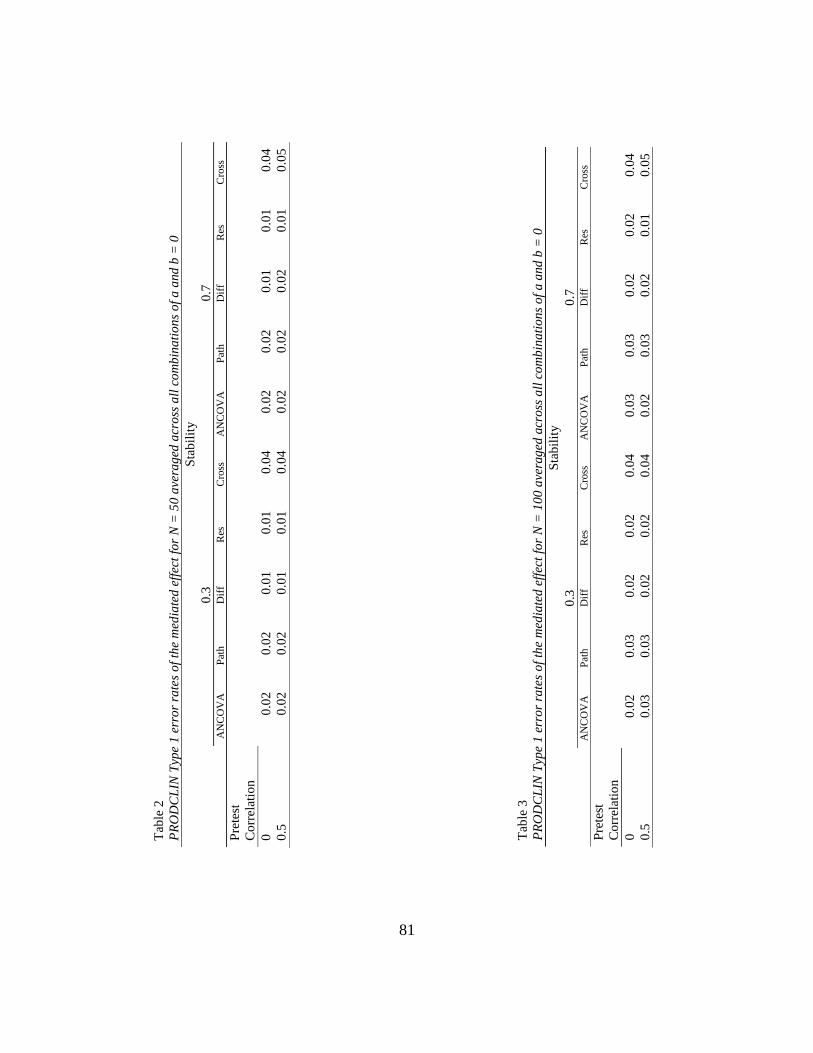
81
T
able
2
PR
OD
CL
IN T
ype
1 e
rro
r ra
tes
of
the
med
iate
d e
ffec
t fo
r N
= 5
0 a
vera
ged
acr
oss
all
co
mb
ina
tio
ns
of
a a
nd
b =
0
Sta
bil
ity
0.3
0
.7
AN
CO
VA
P
ath
Dif
f R
es
Cro
ss
AN
CO
VA
P
ath
Dif
f R
es
Cro
ss
Pre
test
Co
rrel
atio
n
0.0
2
0.0
2
0.0
1
0.0
1
0.0
4
0.0
2
0.0
2
0.0
1
0.0
1
0.0
4
0
0.5
0
.02
0.0
2
0.0
1
0.0
1
0.0
4
0.0
2
0.0
2
0.0
2
0.0
1
0.0
5
Tab
le 3
PR
OD
CL
IN T
ype
1 e
rro
r ra
tes
of
the
med
iate
d e
ffec
t fo
r N
= 1
00
ave
rag
ed a
cro
ss a
ll c
om
bin
ati
on
s o
f a a
nd
b =
0
Sta
bil
ity
0.3
0
.7
AN
CO
VA
P
ath
Dif
f R
es
Cro
ss
AN
CO
VA
P
ath
Dif
f R
es
Cro
ss
Pre
test
Co
rrel
atio
n
0.0
2
0.0
3
0.0
2
0.0
2
0.0
4
0.0
3
0.0
3
0.0
2
0.0
2
0.0
4
0
0.5
0
.03
0.0
3
0.0
2
0.0
2
0.0
4
0.0
2
0.0
3
0.0
2
0.0
1
0.0
5

82
Tab
le 4
PR
OD
CL
IN T
ype
1 e
rro
r ra
tes
of
the
med
iate
d e
ffec
t fo
r N
= 2
00
ave
rag
ed a
cro
ss a
ll c
om
bin
ati
on
s o
f a a
nd
b =
0
Sta
bil
ity
0.3
0
.7
AN
CO
VA
P
ath
Dif
f R
es
Cro
ss
AN
CO
VA
P
ath
Dif
f R
es
Cro
ss
Pre
test
Co
rrel
atio
n
0.0
3
0.0
3
0.0
3
0.0
2
0.0
4
0.0
3
0.0
3
0.0
2
0.0
2
0.0
4
0
0.5
0
.03
0.0
3
0.0
3
0.0
2
0.0
5
0.0
3
0.0
3
0.0
3
0.0
2
0.0
5
Tab
le 5
PR
OD
CL
IN T
ype
1 e
rro
r ra
tes
of
the
med
iate
d e
ffec
t fo
r N
= 5
00
ave
rag
ed a
cro
ss a
ll c
om
bin
ati
on
s o
f a a
nd
b =
0
Sta
bil
ity
0.3
0
.7
AN
CO
VA
P
ath
Dif
f R
es
Cro
ss
AN
CO
VA
P
ath
Dif
f R
es
Cro
ss
Pre
test
Co
rrel
atio
n
0.0
3
0.0
3
0.0
4
0.0
3
0.0
5
0.0
3
0.0
3
0.0
3
0.0
3
0.0
5
0
0.5
0
.03
0.0
3
0.0
4
0.0
3
0.0
5
0.0
3
0.0
3
0.0
3
0.0
3
0.0
5

83
Tab
le 6
Bia
s, R
ela
tive
bia
s, a
nd
Sta
nda
rdiz
ed b
ias
of
the
med
iate
d e
ffec
t fo
r th
e A
NC
OV
A m
od
el
N
50
10
0
20
0
50
0
Bia
s
Rel
Bia
s
Sta
nd
Bia
s B
ias
Rel
Bia
s
Sta
nd
Bia
s B
ias
Rel
Bia
s
Sta
nd
Bia
s B
ias
Rel
Bia
s
Sta
nd
Bia
s
Tru
e
Val
ue
0.0
0
N/A
0
.00
0.0
0
N/A
0
.00
0.0
0
N/A
0
.01
0.0
0
N/A
0
.00
0
0.0
1
0.0
0
0.0
3
0.0
1
0.0
0
-0.0
2
-0.0
1
0.0
0
-0.0
1
-0.0
1
0.0
0
0.0
0
0.0
0
0.0
3
0.0
0
-0.0
2
-0.0
1
0.0
0
0.0
1
0.0
0
0.0
0
0.0
0
0.0
1
0.0
0
-0.0
1
-0.0
2
0.0
5
0.0
0
-0.0
1
-0.0
1
0.0
0
0.0
0
0.0
0
0.0
0
0.0
0
0.0
0
0.0
0
0.0
1
0.0
1
0.0
9
0.0
0
0.0
0
-0.0
0
0.0
0
0.0
0
0.0
0
0.0
0
0.0
0
0.0
0
0.0
0
0.0
0
0.0
0
0.1
5
0.0
0
0.0
0
0.0
1
0.0
0
0.0
0
0.0
0
0.0
0
0.0
0
0.0
1
0.0
0
0.0
0
0.0
0
0.2
5
0.0
0
0.0
0
0.0
1
0.0
0
0.0
0
-0.0
1
0.0
0
0.0
0
-0.0
1
0.0
0
0.0
0
0.0
1
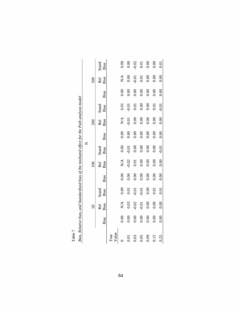
84
Tab
le 7
Bia
s, R
ela
tive
bia
s, a
nd
Sta
nda
rdiz
ed b
ias
of
the
med
iate
d e
ffec
t fo
r th
e P
ath
ana
lysi
s m
od
el
N
50
10
0
20
0
50
0
Bia
s
Rel
Bia
s
Sta
nd
Bia
s B
ias
Rel
Bia
s
Sta
nd
Bia
s B
ias
Rel
Bia
s
Sta
nd
Bia
s B
ias
Rel
Bia
s
Sta
nd
Bia
s
Tru
e
Val
ue
0.0
0
N/A
0
.00
0.0
0
N/A
0
.00
0.0
0
N/A
0
.01
0.0
0
N/A
0
.00
0
0.0
1
0.0
0
0.0
3
0.0
1
0.0
0
-0.0
2
-0.0
1
0.0
0
-0.0
1
-0.0
1
0.0
0
0.0
0
0.0
0
0.0
3
0.0
0
-0.0
2
-0.0
1
0.0
0
0.0
1
0.0
0
0.0
0
0.0
0
0.0
1
0.0
0
-0.0
1
-0.0
2
0.0
5
0.0
0
-0.0
1
-0.0
1
0.0
0
0.0
0
0.0
0
0.0
0
0.0
0
0.0
0
0.0
0
0.0
1
0.0
1
0.0
9
0.0
0
0.0
0
0.0
0
0.0
0
0.0
0
0.0
0
0.0
0
0.0
0
0.0
0
0.0
0
0.0
0
0.0
0
0.1
5
0.0
0
0.0
0
0.0
1
0.0
0
0.0
0
0.0
0
0.0
0
0.0
0
0.0
1
0.0
0
0.0
0
0.0
0
0.2
5
0.0
0
0.0
0
0.0
1
0.0
0
0.0
0
-0.0
1
0.0
0
0.0
0
-0.0
1
0.0
0
0.0
0
0.0
1

85
Tab
le 8
Bia
s, R
ela
tive
bia
s, a
nd
Sta
nda
rdiz
ed b
ias
of
the
med
iate
d e
ffec
t fo
r th
e D
iffe
ren
ce s
core
mo
del
N
50
10
0
20
0
50
0
Bia
s R
el B
ias
Sta
nd
Bia
s B
ias
Rel
Bia
s S
tand
Bia
s B
ias
Rel
Bia
s S
tand
Bia
s B
ias
Rel
Bia
s S
tand
Bia
s
Tru
e V
alue
0.0
0
N/A
0
.00
0.0
0
N/A
0
.01
0.0
0
N/A
0
.00
0.0
0
N/A
0
.00
0
0.0
1
0.0
0
0.0
1
-0.0
1
0.0
0
0.0
0
-0.0
1
0.0
0
0.0
1
0.0
1
0.0
0
0.0
0
0.0
0
0.0
3
0.0
0
0.0
7
-0.0
2
0.0
0
0.0
6
0.0
0
0.0
0
-0.0
2
0.0
0
0.0
0
0.0
0
-0.0
1
0.0
5
0.0
0
-0.0
0
-0.0
1
0.0
0
-0.0
0
-0.0
1
0.0
0
0.0
0
0.0
1
0.0
0
0.0
1
0.0
1
0.0
9
0.0
0
-0.0
8
0.0
0
0.0
0
0.0
2
-0.0
1
0.0
0
-0.0
1
0.0
1
0.0
0
0.0
0
0.0
0
0.1
5
0.0
0
0.0
1
0.0
1
0.0
0
0.0
1
0.0
0
0.0
0
0.0
0
0.0
1
0.0
0
0.0
0
0.0
0
0.2
5
0.0
0
-0.0
1
0.0
0
0.0
0
0.0
0
0.0
0
0.0
0
0.0
0
-0.0
1
0.0
0
0.0
0
0.0
0

86
Tab
le 9
Bia
s, r
ela
tive
bia
s, a
nd
sta
nd
ard
ized
bia
s o
f th
e m
edia
ted
eff
ect
for
the
resi
du
ali
zed
ch
an
ge s
core
mo
del
wh
en p
rete
st
corr
ela
tio
n =
0.0
0
N
50
10
0
20
0
50
0
Bia
s R
el B
ias
Sta
nd
Bia
s B
ias
Rel
Bia
s
Sta
nd
Bia
s B
ias
Rel
Bia
s
Sta
nd
Bia
s B
ias
Rel
Bia
s
Sta
nd
Bia
s
Tru
e V
alue
0.0
0
N/A
0
.00
0.0
0
N/A
-0
.01
0
.00
N/A
0
.00
0.0
0
N/A
0
.01
0
0.0
1
-0.0
1
-0.3
0
-0.1
1
-0.0
1
-0.3
4
-0.2
2
-0.0
1
-0.2
9
-0.3
0
-0.0
1
-0.2
9
-0.5
2
0.0
3
-0.0
2
-0.3
1
-0.2
1
-0.0
2
-0.2
4
-0.2
4
-0.0
2
-0.2
9
-0.4
5
-0.0
2
-0.2
8
-0.6
8
0.0
5
-0.0
4
-0.3
1
-0.2
5
-0.0
3
-0.2
7
-0.3
0
-0.0
3
-0.2
9
-0.4
6
-0.0
3
-0.2
6
-0.6
8
0.0
9
-0.0
6
-0.3
1
-0.5
0
-0.0
5
-0.2
7
-0.6
6
-0.0
5
-0.2
7
-0.9
9
-0.0
5
-0.2
7
-1.4
9
0.1
5
-0.1
1
-0.2
9
-0.6
0
-0.1
0
-0.2
9
-0.8
7
-0.1
0
-0.2
7
-1.1
9
-0.1
0
-0.2
6
-1.8
2
0.2
5
-0.1
9
-0.2
9
-0.7
8
-0.1
9
-0.2
9
-1.1
3
-0.1
8
-0.2
7
-1.5
2
-0.1
8
-0.2
7
-2.3
8
No
te.
bm
2y1
and
by2
m1
pat
hs
= 0
.50
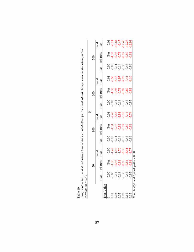
87
Tab
le 1
0
Bia
s, r
ela
tive
bia
s, a
nd
sta
nd
ard
ized
bia
s o
f th
e m
edia
ted
eff
ect
for
the
resi
du
ali
zed
ch
an
ge s
core
mo
del
wh
en p
rete
st
corr
ela
tio
n =
0.5
0
N
50
10
0
20
0
50
0
Bia
s R
el B
ias
Sta
nd
Bia
s B
ias
Rel
Bia
s
Sta
nd
Bia
s B
ias
Rel
Bia
s
Sta
nd
Bia
s B
ias
Rel
Bia
s
Sta
nd
Bia
s
Tru
e V
alue
0.0
0
N/A
0
.00
0.0
0
N/A
-0
.01
0
.00
N/A
0
.01
0.0
0
N/A
0
.01
0
0.0
1
-0.0
8
-1.3
0
-1.4
2
-0.0
9
-1.3
4
-2.4
0
-0.0
9
-1.3
3
-3.5
0
-0.0
9
-1.3
3
-6.1
4
0.0
3
-0.1
1
-0.9
6
-1.9
7
-0.1
1
-0.9
7
-3.4
3
-0.1
1
-0.9
6
-6.1
8
-0.1
1
-0.9
6
-10
.84
0.0
5
-0.1
4
-0.8
1
-1.7
0
-0.1
4
-0.8
2
-2.8
1
-0.1
4
-0.7
9
-3.9
7
-0.1
4
-0.7
9
-6.4
7
0.0
9
-0.3
5
-0.9
6
-3.3
0
-0.3
5
-0.9
7
-5.1
0
-0.3
5
-0.9
7
-7.7
9
-0.3
5
-0.9
7
-12
.46
0.1
5
-0.4
5
-0.8
1
-3.4
1
-0.4
5
-0.8
0
-5.1
4
-0.4
5
-0.8
0
-7.4
1
-0.4
5
-0.8
0
-12
.25
0.2
5
-0.8
5
-0.8
2
-3.7
7
-0.8
6
-0.8
2
-5.7
4
-0.8
5
-0.8
2
-8.1
0
-0.8
6
-0.8
2
-12
.91
No
te.
bm
2y1
and
by2
m1
pat
hs
= 0
.50

88
Tab
le 1
1
Bia
s, R
ela
tive
bia
s, a
nd
Sta
nda
rdiz
ed b
ias
of
the
med
iate
d e
ffec
t fo
r C
ross
-sec
tio
na
l m
od
el w
hen
dir
ect
effe
ct =
0.0
0
N
50
10
0
20
0
50
0
Bia
s
Rel
Bia
s
Sta
nd
Bia
s B
ias
Rel
Bia
s
Sta
nd
Bia
s B
ias
Rel
Bia
s
Sta
nd
Bia
s B
ias
Rel
Bia
s
Sta
nd
Bia
s
by2
m1
T
rue
Val
ue
0.0
0
N/A
0
.00
0.0
0
N/A
0
.00
0.0
0
N/A
0
.00
0.0
0
N/A
0
.00
0
0
0.0
1
0.0
3
1.4
3
0.2
1
0.0
3
1.3
8
0.3
2
0.0
3
1.3
9
0.4
5
0.0
3
1.4
0
0.7
2
0.0
3
0.0
3
0.4
4
0.1
3
0.0
3
0.4
7
0.1
9
0.0
3
0.4
6
0.2
7
0.0
3
0.4
5
0.4
3
0.0
5
0.0
3
0.2
4
0.0
8
0.0
3
0.2
7
0.1
4
0.0
3
0.2
9
0.2
0
0.0
3
0.2
8
0.3
2
0.0
9
0.0
9
0.4
7
0.3
9
0.0
9
0.4
7
0.5
5
0.0
9
0.4
8
0.8
1
0.0
9
0.4
7
1.2
8
0.1
5
0.1
0
0.2
8
0.2
9
0.1
0
0.2
7
0.4
2
0.1
0
0.2
7
0.5
8
0.1
0
0.2
7
0.9
1
0.2
5
0.1
9
0.2
8
0.4
9
0.1
9
0.2
8
0.6
9
0.1
8
0.2
8
0.9
6
0.1
9
0.2
8
1.5
7
0.5
0
0
.00
N/A
0
.00
0.0
0
N/A
0
.00
0.0
0
N/A
0
.00
0.0
0
N/A
-0
.01
0.0
1
0.1
0
4.8
9
0.4
1
0.1
0
4.8
4
0.5
8
0.1
0
4.9
2
0.8
6
0.1
0
4.8
8
1.3
6
0.0
3
0.1
0
1.6
3
0.3
1
0.1
1
1.6
9
0.4
7
0.1
0
1.5
9
0.6
4
0.1
0
1.5
6
0.9
8
0.0
5
0.1
0
0.8
5
0.2
3
0.1
0
0.8
8
0.3
4
0.1
0
0.8
6
0.4
7
0.1
0
0.8
9
0.7
7
0.0
9
0.3
2
1.5
9
0.8
9
0.3
2
1.6
2
1.3
2
0.3
2
1.6
1
1.8
7
0.3
2
1.6
1
2.9
9
0.1
5
0.3
3
0.9
0
0.7
1
0.3
2
0.8
8
1.0
1
0.3
2
0.8
9
1.4
5
0.3
2
0.8
9
2.2
9
0.2
5
0.6
1
0.9
1
1.2
0
0.6
1
0.9
2
1.7
4
0.6
2
0.9
2
2.4
6
0.6
2
0.9
2
3.8
9

89
Tab
le 1
2
Bia
s, R
ela
tive
bia
s, a
nd
Sta
nda
rdiz
ed b
ias
of
the
med
iate
d e
ffec
t fo
r th
e C
ross
-sec
tio
na
l m
od
el w
hen
dir
ect
effe
ct =
0.3
0 a
nd
N =
50
bm
2y1
0
0.5
by2
m1
by2
m1
0
0.5
0
0
.5
Bia
s R
el B
ias
Sta
nd
Bia
s B
ias
Rel
Bia
s
Sta
nd
Bia
s B
ias
Rel
Bia
s
Sta
nd
Bia
s B
ias
Rel
Bia
s
Sta
nd
Bia
s
Pre
test
Co
rrel
atio
n T
rue
Val
ue
0.0
0
0.0
6
0.0
2
0.0
7
3.6
6
0.4
2
0.0
4
1.8
8
0.3
1
0.0
9
4.6
1
0.4
0
0
0.0
1
0.0
9
0.0
0
0.0
0
0.0
0
0.2
4
1.2
2
0.8
6
0.1
1
0.5
7
0.5
2
0.2
9
1.4
9
0.8
7
0.2
5
0.0
0
0.0
1
0.0
1
0.4
6
0.6
9
1.0
7
0.1
9
0.2
8
0.5
4
0.5
8
0.8
7
1.2
2
0.5
0
.01
0.0
2
1.2
1
0.2
2
0.1
1
5.1
9
0.4
3
0.0
5
2.5
6
0.3
1
0.1
3
6.2
3
0.3
9
0.0
9
0.0
9
0.4
7
0.4
3
0.3
3
1.6
9
0.9
4
0.1
8
0.9
1
0.6
3
0.4
0
2.0
3
0.9
1
0.2
5
0.2
0
0.3
1
0.5
8
0.6
4
0.9
6
1.2
8
0.3
5
0.5
3
0.8
0
0.7
6
1.1
3
1.2
5
Tab
le 1
3
Bia
s, R
ela
tive
bia
s, a
nd
Sta
nda
rdiz
ed b
ias
of
the
med
iate
d e
ffec
t fo
r th
e C
ross
-sec
tio
na
l m
od
el w
hen
dir
ect
effe
ct =
0.3
0 a
nd
N =
100
bm
2y1
0
0.5
by2
m1
by2
m1
0
0.5
0
0
.5
Bia
s R
el B
ias
Sta
nd
Bia
s B
ias
Rel
Bia
s
Sta
nd
Bia
s B
ias
Rel
Bia
s
Sta
nd
Bia
s B
ias
Rel
Bia
s
Sta
nd
Bia
s
Pre
test
Co
rrel
atio
n T
rue
Val
ue
0.0
0
0.0
2
0.0
1
0.0
7
3.5
8
0.5
8
0.0
3
1.7
0
0.4
3
0.0
9
4.5
3
0.5
5
0
0.0
1
0.0
9
0.0
0
-0.0
2
-0.0
4
0.2
4
1.2
1
1.2
5
0.1
1
0.5
6
0.7
5
0.3
2
1.6
0
1.3
2
0.2
5
0.0
0
-0.0
0
-0.0
1
0.4
5
0.6
8
1.5
6
0.2
1
0.3
2
0.9
0
0.6
0
0.8
9
1.7
5
0.5
0
.01
0.0
3
1.3
4
0.3
7
0.1
0
4.9
7
0.6
2
0.0
5
2.5
6
0.4
5
0.1
2
5.9
7
0.5
4
0.0
9
0.1
0
0.4
8
0.6
3
0.3
3
1.6
5
1.3
9
0.1
7
0.8
6
0.8
2
0.4
1
2.0
7
1.3
5
0.2
5
0.2
0
0.3
0
0.8
0
0.6
8
1.0
1
1.9
2
0.3
5
0.5
2
1.0
9
0.8
0
1.1
9
1.8
8
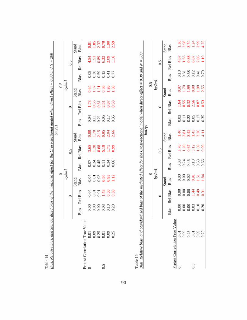
90
Tab
le 1
4
Bia
s, R
ela
tive
bia
s, a
nd
Sta
nda
rdiz
ed b
ias
of
the
med
iate
d e
ffec
t fo
r th
e C
ross
-sec
tio
na
l m
od
el w
hen
dir
ect
effe
ct =
0.3
0 a
nd
N =
200
bm
2y1
0
0.5
by2
m1
by2
m1
0
0.5
0
0
.5
Bia
s R
el B
ias
Sta
nd
Bia
s B
ias
Rel
Bia
s
Sta
nd
Bia
s B
ias
Rel
Bia
s
Sta
nd
Bia
s B
ias
Rel
Bia
s
Sta
nd
Bia
s
Pre
test
Co
rrel
atio
n T
rue
Val
ue
0.0
0
-0.0
4
-0.0
4
0.0
7
3.6
5
0.8
8
0.0
4
1.7
3
0.6
4
0.0
9
4.5
4
0.8
1
0
0.0
1
0.0
9
0.0
0
0.0
1
0.0
1
0.2
4
1.2
0
1.7
0
0.1
1
0.5
6
1.0
7
0.3
0
1.5
1
1.8
5
0.2
5
0.0
0
-0.0
1
-0.0
3
0.4
5
0.6
8
2.1
5
0.2
1
0.3
1
1.2
1
0.5
9
0.8
9
2.3
7
0.5
0
.01
0.0
3
1.4
3
0.5
6
0.1
1
5.1
9
0.9
5
0.0
5
2.5
1
0.6
0
0.1
3
6.2
2
0.7
9
0.0
9
0.1
0
0.5
0
0.9
3
0.3
4
1.7
1
2.0
4
0.1
7
0.8
7
1.2
6
0.4
1
2.0
9
1.9
0
0.2
5
0.2
0
0.3
0
1.1
2
0.6
6
0.9
9
2.6
6
0.3
5
0.5
3
1.6
0
0.7
7
1.1
6
2.5
9
Tab
le 1
5
Bia
s, R
ela
tive
bia
s, a
nd
Sta
nda
rdiz
ed b
ias
of
the
med
iate
d e
ffec
t fo
r th
e C
ross
-sec
tio
na
l m
od
el w
hen
dir
ect
effe
ct =
0.3
0 a
nd
N =
500
bm
2y1
0
0.5
by2
m1
by2
m1
0
0.5
0
0
.5
Bia
s R
el B
ias
Sta
nd
Bia
s B
ias
Rel
Bia
s
Sta
nd
Bia
s B
ias
Rel
Bia
s
Sta
nd
Bia
s B
ias
Rel
Bia
s
Sta
nd
Bia
s
Pre
test
Co
rrel
atio
n T
rue
Val
ue
0.0
0
0.0
0
0.0
0
0.0
8
3.7
6
1.4
0
0.0
3
1.6
4
0.9
7
0.1
0
4.6
7
1.3
6
0
0.0
1
0.0
9
0.0
0
0.0
0
0.0
0
0.2
4
1.2
0
2.8
1
0.1
1
0.5
5
1.7
0
0.3
1
1.5
5
2.9
8
0.2
5
0.0
0
0.0
0
0.0
2
0.4
5
0.6
7
3.4
2
0.2
2
0.3
2
1.9
9
0.5
8
0.8
8
3.7
4
0.5
0
.01
0.0
3
1.4
4
0.9
1
0.1
0
5.1
2
1.4
5
0.0
5
2.5
6
0.9
8
0.1
2
6.0
7
1.2
4
0.0
9
0.1
0
0.4
9
1.5
1
0.3
3
1.6
9
3.2
6
0.1
7
0.8
7
1.9
8
0.4
1
2.0
6
2.9
9
0.2
5
0.2
0
0.3
1
1.8
4
0.6
6
0.9
9
4.1
1
0.3
5
0.5
3
2.5
5
0.7
9
1.1
9
4.2
5

91
Table 16
PRODCLIN 95% Confidence interval coverage of the
mediated effect for the ANCOVA model
N
50 100 200 500
95% C.I.
Coverage
95% C.I.
Coverage
95% C.I.
Coverage
95% C.I.
Coverage
True Value
0.980 0.975 0.973 0.968 0
0.01 0.994 0.992 0.974 0.948
0.03 0.971 0.948 0.950 0.949
0.05 0.945 0.946 0.948 0.951
0.09 0.943 0.946 0.952 0.950
0.15 0.945 0.948 0.949 0.951
0.25 0.946 0.950 0.949 0.950
Table 17
PRODCLIN 95% confidence interval coverage of the
mediated effect for the Path analysis model
N
50 100 200 500
95% C.I.
Coverage
95% C.I.
Coverage
95% C.I.
Coverage
95% C.I.
Coverage
True Value
0.975 0.973 0.972 0.955 0
0.01 0.992 0.990 0.971 0.947
0.03 0.962 0.945 0.949 0.948
0.05 0.937 0.942 0.947 0.950
0.09 0.933 0.942 0.936 0.949
0.15 0.937 0.945 0.947 0.950
0.25 0.937 0.946 0.931 0.949

92
Table 18
PRODCLIN 95% confidence interval coverage of the
mediated effect for the Difference score model
N
50 100 200 500
95% C.I.
Coverage
95% C.I.
Coverage
95% C.I.
Coverage
95% C.I.
Coverage
True Value
0.986 0.980 0.974 0.966 0
0.01 0.991 0.983 0.971 0.954
0.03 0.983 0.971 0.963 0.953
0.05 0.970 0.962 0.957 0.950
0.09 0.955 0.950 0.951 0.948
0.15 0.956 0.952 0.950 0.950
0.25 0.948 0.948 0.950 0.950

93
Tab
le 1
9
PR
OD
CL
IN 9
5%
co
nfi
den
ce i
nte
rva
l co
vera
ge o
f th
e m
edia
ted
eff
ect
for
the
resi
du
ali
zed
ch
an
ge
sco
re m
od
el w
hen
Dir
ect
effe
ct =
0.0
0,
N =
50
, a
nd
N
= 1
00
N
50
10
0
bm
2y1
b
m2
y1
0
0.5
0
0
.5
by2
m1
by2
m1
by2
m1
by2
m1
0
0.5
0
0
.5
0
0.5
0
0
.5
95
% C
.I.
Co
ver
age
95
% C
.I.
Co
ver
age
95
% C
.I.
Co
ver
age
95
% C
.I.
Co
ver
age
95
% C
.I.
Co
ver
age
95
% C
.I.
Co
ver
age
95
% C
.I.
Co
ver
age
95
% C
.I.
Co
ver
age
Pre
test
Co
rr.
Tru
e V
alue
0.9
80
0.9
92
0.9
85
0.9
93
0
.97
8
0.9
81
0.9
79
0.9
88
0
0
0.0
1
0.9
95
0.9
99
0.9
97
0.9
98
0
.99
1
1.0
00
0.9
95
0.9
98
0.0
3
0.9
70
0.9
89
0.9
77
0.9
90
0
.94
3
0.9
65
0.9
37
0.9
62
0.0
5
0.9
50
0.9
72
0.9
32
0.9
59
0
.94
4
0.9
60
0.9
36
0.9
32
0.0
9
0.9
39
0.9
76
0.9
17
0.9
39
0
.94
9
0.9
82
0.8
85
0.9
37
0.1
5
0.9
53
0.9
72
0.8
97
0.9
18
0
.95
7
0.9
66
0.8
65
0.8
95
0.2
5
0.9
43
0.9
75
0.8
54
0.9
15
0
.95
1
0.9
79
0.7
69
0.8
65
0.5
0
0
.98
1
0.9
89
0.9
89
0.9
98
0
.97
7
0.9
82
0.9
84
0.9
93
0.0
1
0.9
95
0.9
99
0.9
96
0.9
64
0
.99
4
0.9
98
0.9
94
0.4
86
0.0
3
0.9
65
0.9
82
0.9
50
0.8
96
0
.94
1
0.9
62
0.8
65
0.3
55
0.0
5
0.9
39
0.9
55
0.8
84
0.7
32
0
.95
1
0.9
56
0.8
51
0.4
75
0.0
9
0.9
39
0.9
62
0.7
77
0.2
96
0
.94
4
0.9
66
0.6
60
0.0
59
0.1
5
0.9
40
0.9
49
0.7
17
0.3
29
0
.94
5
0.9
66
0.5
43
0.0
86
0.2
5
0.9
47
0.9
68
0.5
54
0.1
65
0
.94
4
0.9
71
0.3
13
0.0
15

94
Tab
le 2
0
PR
OD
CL
IN 9
5%
co
nfi
den
ce i
nte
rva
l co
vera
ge o
f th
e m
edia
ted
eff
ect
for
the
resi
du
ali
zed
ch
an
ge
sco
re m
od
el w
hen
Dir
ect
effe
ct =
0.0
, N
= 2
00
, a
nd
N
= 5
00
N
20
0
50
0
bm
2y1
b
m2
y1
0
0.5
0
0
.5
by2
m1
by2
m1
by2
m1
by2
m1
0
0.5
0
0
.5
0
0.5
0
0
.5
95
% C
.I.
Co
ver
age
95
% C
.I.
Co
ver
age
95
% C
.I.
Co
ver
age
95
% C
.I.
Co
ver
age
95
% C
.I.
Co
ver
age
95
% C
.I.
Co
ver
age
95
% C
.I.
Co
ver
age
95
% C
.I.
Co
ver
age
Pre
test
Co
rr.
Tru
e V
alue
0.9
73
0.9
80
0.9
75
0.9
79
0.9
67
0
.97
1
0.9
70
0.9
73
0
0
0.0
1
0.9
75
0.9
93
0.9
78
0.9
97
0.9
40
0
.97
1
0.9
22
0.9
36
0.0
3
0.9
58
0.9
68
0.9
27
0.9
25
0.9
55
0
.96
5
0.8
95
0.8
95
0.0
5
0.9
40
0.9
55
0.9
21
0.9
23
0.9
52
0
.96
2
0.8
94
0.9
02
0.0
9
0.9
59
0.9
83
0.8
39
0.9
18
0.9
58
0
.98
8
0.6
88
0.8
19
0.1
5
0.9
58
0.9
79
0.7
98
0.8
42
0.9
54
0
.98
4
0.5
69
0.6
74
0.2
5
0.9
56
0.9
78
0.6
33
0.7
69
0.9
63
0
.97
9
0.2
79
0.4
97
0.5
0
0
.97
5
0.9
77
0.9
76
0.9
86
0.9
71
0
.97
2
0.9
72
0.9
75
0.0
1
0.9
73
0.9
92
0.9
12
0.0
81
0.9
51
0
.96
8
0.8
12
0.0
00
0.0
3
0.9
55
0.9
55
0.8
12
0.0
91
0.9
53
0
.94
6
0.6
30
0.0
02
0.0
5
0.9
51
0.9
53
0.7
87
0.2
37
0.9
46
0.9
49
0.5
74
0.0
18
0.0
9
0.9
52
0.9
69
0.4
97
0.0
02
0.9
53
0
.97
3
0.1
81
0.0
00
0.1
5
0.9
48
0.9
70
0.3
06
0.0
05
0.9
55
0
.96
8
0.0
71
0.0
00
0.2
5
0.9
57
0.9
66
0.1
22
0.0
00
0.9
59
0
.97
2
0.0
05
0.0
00

95
Tab
le 2
1
PR
OD
CL
IN 9
5%
co
nfi
den
ce i
nte
rva
l co
vera
ge o
f th
e m
edia
ted
eff
ect
for
the
resi
du
ali
zed
ch
an
ge
sco
re m
od
el w
hen
Dir
ect
effe
ct =
0.3
0,
N =
50
, a
nd
N
= 1
00
N
50
10
0
bm
2y1
b
m2
y1
0
0.5
0
0
.5
by2
m1
by2
m1
by2
m1
by2
m1
0
0.5
0
0
.5
0
0.5
0
0
.5
95
% C
.I.
Co
ver
age
95
% C
.I.
Co
ver
age
95
% C
.I.
Co
ver
age
95
% C
.I.
Co
ver
age
95
% C
.I.
Co
ver
age
95
% C
.I.
Co
ver
age
95
% C
.I.
Co
ver
age
95
% C
.I.
Co
ver
age
Pre
test
Co
rr.
Tru
e V
alue
0.9
96
0.9
97
1.0
00
1.0
00
0
.99
1
0.9
99
0.9
96
1.0
00
0
0.0
1
0.0
9
0.9
49
0.9
74
0.9
12
0.9
44
0
.94
1
0.9
80
0.8
96
0.9
40
0.2
5
0.9
40
0.9
76
0.8
34
0.9
16
0
.95
9
0.9
82
0.8
10
0.8
80
0.5
0
.01
0.9
93
0.9
98
0.9
98
0.9
62
0
.99
0
0.9
96
0.9
92
0.4
64
0.0
9
0.9
48
0.9
61
0.8
02
0.3
07
0
.93
8
0.9
78
0.6
79
0.0
64
0.2
5
0.9
47
0.9
61
0.5
56
0.1
67
0.9
55
0.9
72
0.3
14
0.0
13

96
Tab
le 2
2
PR
OD
CL
IN 9
5%
co
nfi
den
ce i
nte
rva
l co
vera
ge o
f th
e m
edia
ted
eff
ect
for
the
resi
du
ali
zed
ch
an
ge
sco
re m
od
el w
hen
Dir
ect
Eff
ect
= 0
.30
, N
= 2
00
an
d
N =
50
0
N
20
0
50
0
bm
2y1
b
m2
y1
0
0.5
0
0
.5
by2
m1
by2
m1
by2
m1
by2
m1
0
0.5
0
0
.5
0
0.5
0
0
.5
95
% C
.I.
Co
ver
age
95
% C
.I.
Co
ver
age
95
% C
.I.
Co
ver
age
95
% C
.I.
Co
ver
age
95
% C
.I.
Co
ver
age
95
% C
.I.
Co
ver
age
95
% C
.I.
Co
ver
age
95
% C
.I.
Co
ver
age
Pre
test
Co
rr.
Tru
e V
alue
0.9
72
0.9
99
0.9
73
0.9
95
0.9
49
0.9
78
0.9
06
0
.95
4
0
0.0
1
0.0
9
0.9
50
0.9
84
0.8
48
0.9
19
0.9
54
0.9
82
0.6
92
0
.81
6
0.2
5
0.9
52
0.9
82
0.6
24
0.7
82
0.9
58
0.9
84
0.2
76
0
.48
8
0.5
0
.01
0.9
70
0.9
91
0.9
09
0.0
68
0.9
41
0.9
65
0.8
02
0
.00
1
0.0
9
0.9
47
0.9
73
0.4
89
0.0
01
0.9
53
0.9
70
0.1
76
0
.00
0
0.2
5
0.9
56
0.9
73
0.1
16
0.0
00
0.9
46
0.9
70
0.0
06
0
.00
0

97
Table 23
PRODCLIN 95% confidence interval coverage of the mediated effect for the cross-
sectional model when Direct effect = 0.00
N
50 100 200 500
by2m1 by2m1 by2m1 by2m1
0 0.5 0 0.5 0 0.5 0 0.5
95% C.I.
Coverage
95% C.I.
Coverage
95% C.I.
Coverage
95% C.I.
Coverage
95% C.I.
Coverage
95% C.I.
Coverage
95% C.I.
Coverage
95% C.I.
Coverage
True
Value
0.968 0.952 0.963 0.949 0.958 0.951 0.957 0.949 0
0.01 0.974 0.936 0.958 0.910 0.937 0.861 0.865 0.719
0.03 0.952 0.931 0.943 0.924 0.935 0.902 0.924 0.829
0.05 0.944 0.938 0.944 0.933 0.942 0.924 0.929 0.882
0.09 0.934 0.851 0.909 0.737 0.843 0.522 0.688 0.142
0.15 0.935 0.889 0.930 0.826 0.902 0.689 0.809 0.357
0.25 0.915 0.774 0.875 0.589 0.799 0.281 0.579 0.020
Table 24
PRODCLIN 95% confidence interval coverage of the mediated effect for the cross-
sectional model when Direct effect = 0.30
N
50 100 200 500
by2m1 by2m1 by2m1 by2m1
0 0.5 0 0.5 0 0.5 0 0.5
95% C.I.
Coverage
95% C.I.
Coverage
95% C.I.
Coverage
95% C.I.
Coverage
95% C.I.
Coverage
95% C.I.
Coverage
95% C.I.
Coverage
95% C.I.
Coverage
True
Value
0.973 0.941 0.959 0.907 0.931 0.864 0.869 0.709 0.01
0.09 0.927 0.858 0.903 0.735 0.846 0.518 0.681 0.137
0.25 0.919 0.772 0.878 0.564 0.777 0.276 0.556 0.020

98
Table 25
Comparison of sample size requirement for 0.80 power to detect the cross-
sectional mediated effect across current study and Fritz & MacKinnon (2007)
Study
Fritz & MacKinnon (2007) Current Simulation Study
N Effect size N Effect Size Observed
Empirical Power
57.5 0.23 50 0.25 0.84
105.0 0.15 100 0.15 0.72
124.5 0.10 100 – 200 0.09 0.61 – 0.92
402.5 0.05 200 – 500 0.05 0.21 – 0.44
403.0 0.08 200 – 500 0.09 0.92 – 0.99
533.0 0.02 500 0.03 0.46

99
Table 26
Significance test summary indicator of the mediated effect for the five models
Power Percent Cumulative
Percent
00000 36.18 36.18
00001 3.79 39.97
00010 0.94 40.90
00011 0.99 41.89
00100 0.14 42.03
00101 0.14 42.17
00110 0.19 42.36
00111 0.14 42.50
01001 0.00 42.50
01010 0.00 42.50
01011 0.00 42.50
01100 0.00 42.50
01101 0.00 42.51
01110 0.00 42.51
01111 0.01 42.52
10000 0.29 42.82
10001 0.17 42.98
10010 0.05 43.03
10011 0.05 43.08
10100 0.03 43.11
10101 0.03 43.14
10110 0.03 43.17
10111 0.01 43.18
11000 3.01 46.19
11001 3.47 49.66
11010 1.17 50.83
11011 4.14 54.97
11100 1.09 56.06
11101 10.84 66.90
11110 3.81 70.71
11111 29.29 100.00
Note: Order of indicator is Path analysis, ANCOVA, res. change, diff. score, and cross-sectional

100
Figure 1. Path diagram of pretest posttest control group design with mediating variable.
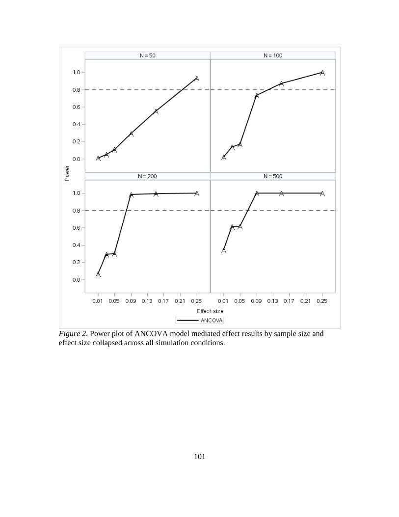
101
Figure 2. Power plot of ANCOVA model mediated effect results by sample size and
effect size collapsed across all simulation conditions.
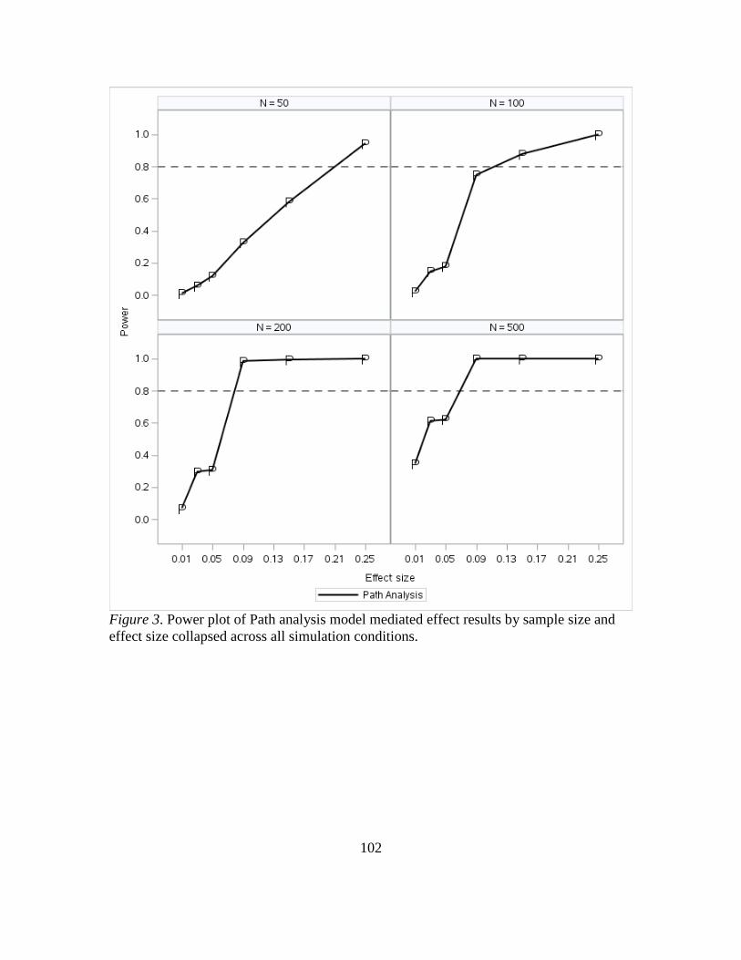
102
Figure 3. Power plot of Path analysis model mediated effect results by sample size and
effect size collapsed across all simulation conditions.
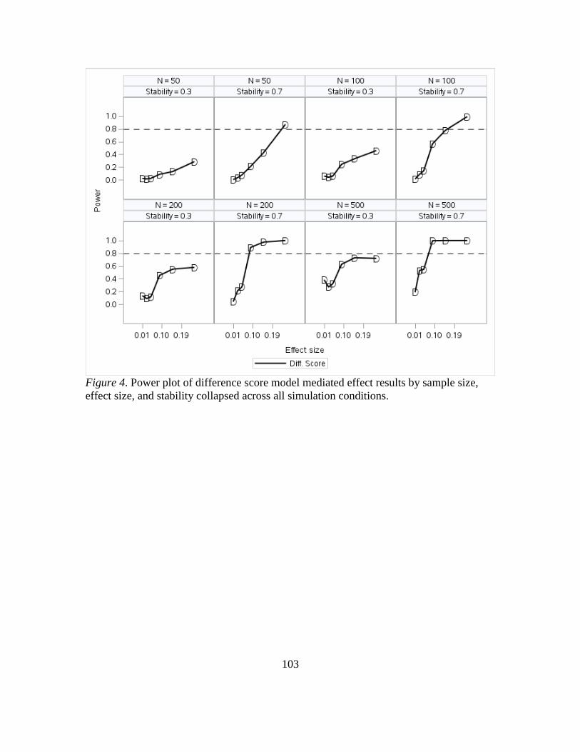
103
Figure 4. Power plot of difference score model mediated effect results by sample size,
effect size, and stability collapsed across all simulation conditions.
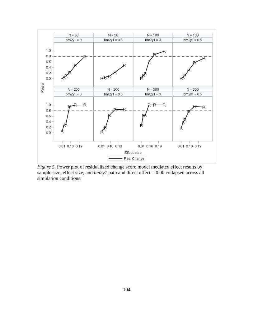
104
Figure 5. Power plot of residualized change score model mediated effect results by
sample size, effect size, and bm2y1 path and direct effect = 0.00 collapsed across all
simulation conditions.

105
Figure 6. Power plot of residualized change score model mediated effect results by effect
size, bm2y1 path, and by2m1 path for sample size N= 50 and N = 100 and direct effect =
0.30 collapsed across all simulation conditions.

106
Figure 7. Power plot of residualized change score model mediated effect results by effect
size, bm2y1 path, and by2m1 path for sample size N= 200 and N = 500 and direct effect =
0.30 collapsed across all simulation conditions.
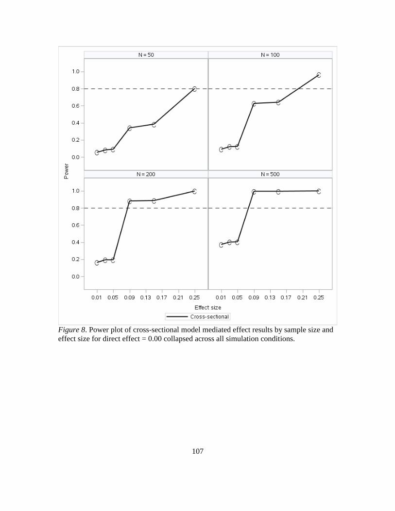
107
Figure 8. Power plot of cross-sectional model mediated effect results by sample size and
effect size for direct effect = 0.00 collapsed across all simulation conditions.

108
Figure 9. Power plot of cross-sectional model mediated effect results by sample size,
effect size, and stability for direct effect = 0.30 collapsed across all simulation conditions.

109
Figure 10. Power plot of ANCOVA vs. cross-sectional model mediated effect results by
sample size and effect size collapsed across all simulation conditions.

110
Figure 11. Power plot of path analysis vs. cross-sectional model mediated effect results
by sample size and effect size collapsed across all simulation conditions.

111
Figure 12. Power plot of difference score model mediated effect results by effect size,
stability, and by2m1 path for sample size N= 50 and N = 100 and direct effect = 0.00
collapsed across all simulation conditions.
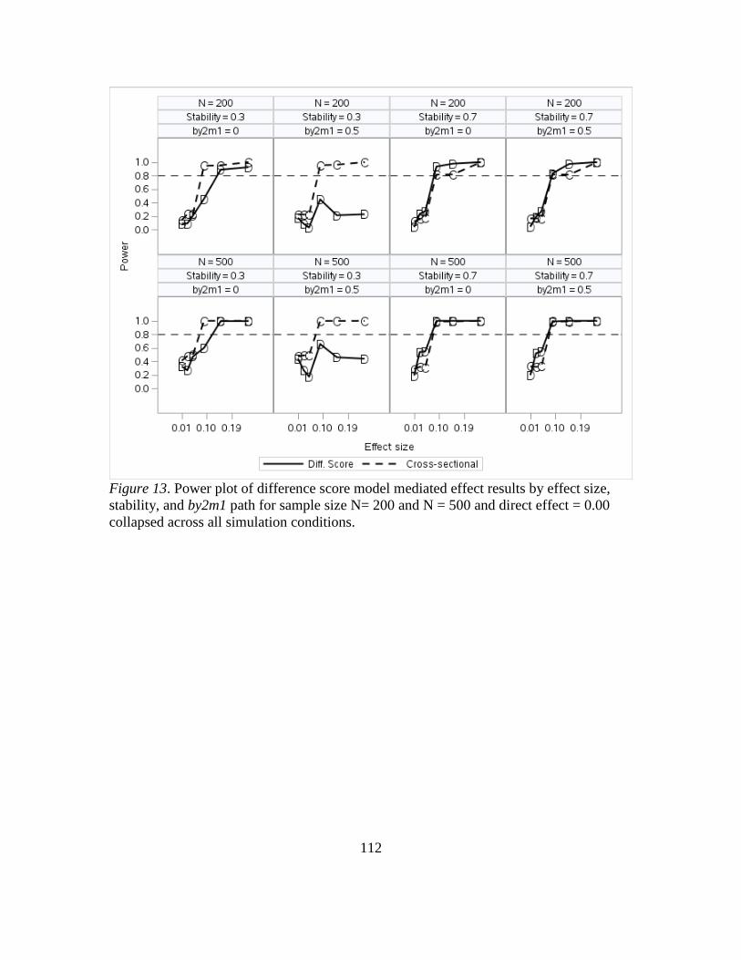
112
Figure 13. Power plot of difference score model mediated effect results by effect size,
stability, and by2m1 path for sample size N= 200 and N = 500 and direct effect = 0.00
collapsed across all simulation conditions.

113
Figure 14. Power plot of difference score vs. cross-sectional model mediated effect
results by effect size, sample size, and stability for direct effect = 0.30 collapsed across
all simulation conditions.

114
Figure 15. Power plot of residualized change score vs. cross-sectional model mediated
effect results by sample size and effect size collapsed across all simulation conditions.

115
Figure 16. Power plot of path analysis vs. difference score model mediated effect results
by sample size, effect size, stability and by2m1 path for N = 50 – 100 and direct effect =
0.00 collapsed across all simulation conditions.

116
Figure 17. Power plot of path analysis vs. difference score model mediated effect results
by sample size, effect size, stability and by2m1 path for N = 200 – 500 and direct effect =
0.00 collapsed across all simulation conditions.
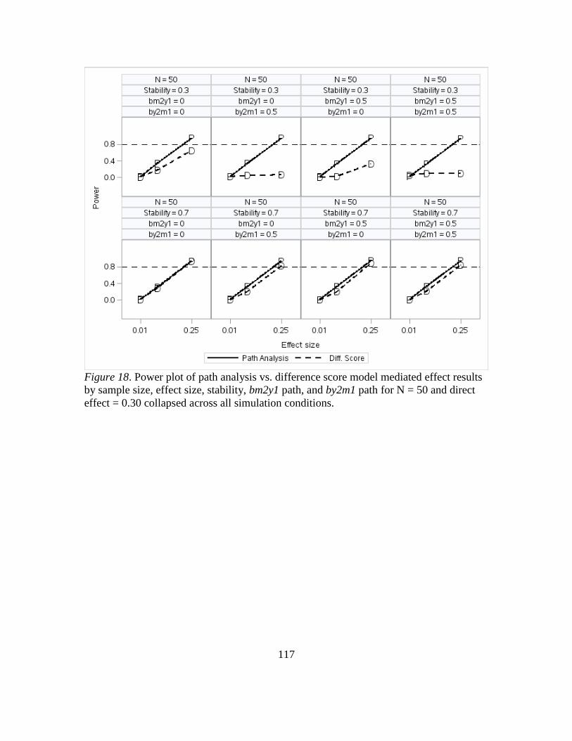
117
Figure 18. Power plot of path analysis vs. difference score model mediated effect results
by sample size, effect size, stability, bm2y1 path, and by2m1 path for N = 50 and direct
effect = 0.30 collapsed across all simulation conditions.
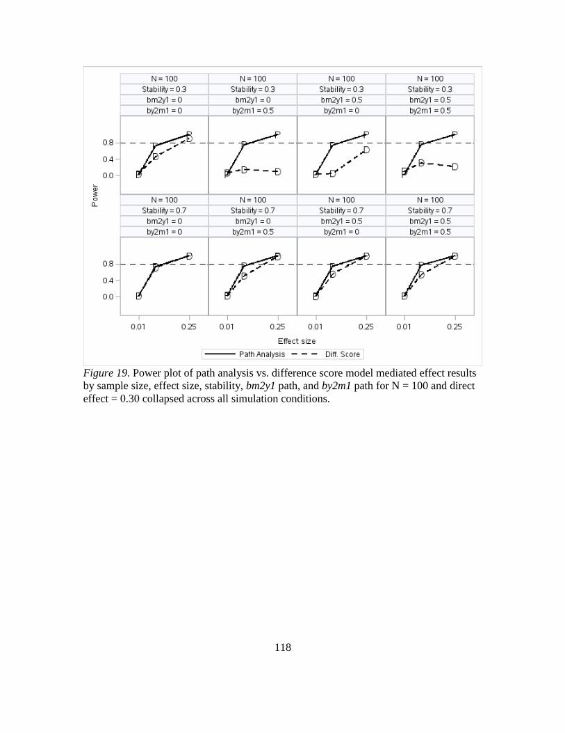
118
Figure 19. Power plot of path analysis vs. difference score model mediated effect results
by sample size, effect size, stability, bm2y1 path, and by2m1 path for N = 100 and direct
effect = 0.30 collapsed across all simulation conditions.

119
Figure 20. Power plot of path analysis vs. difference score model mediated effect results
by sample size, effect size, stability, bm2y1 path, and by2m1 path for N = 200 and direct
effect = 0.30 collapsed across all simulation conditions.

120
Figure 21. Power plot of path analysis vs. difference score model mediated effect results
by sample size, effect size, stability, bm2y1 path, and by2m1 path for N = 500 and direct
effect = 0.30 collapsed across all simulation conditions.
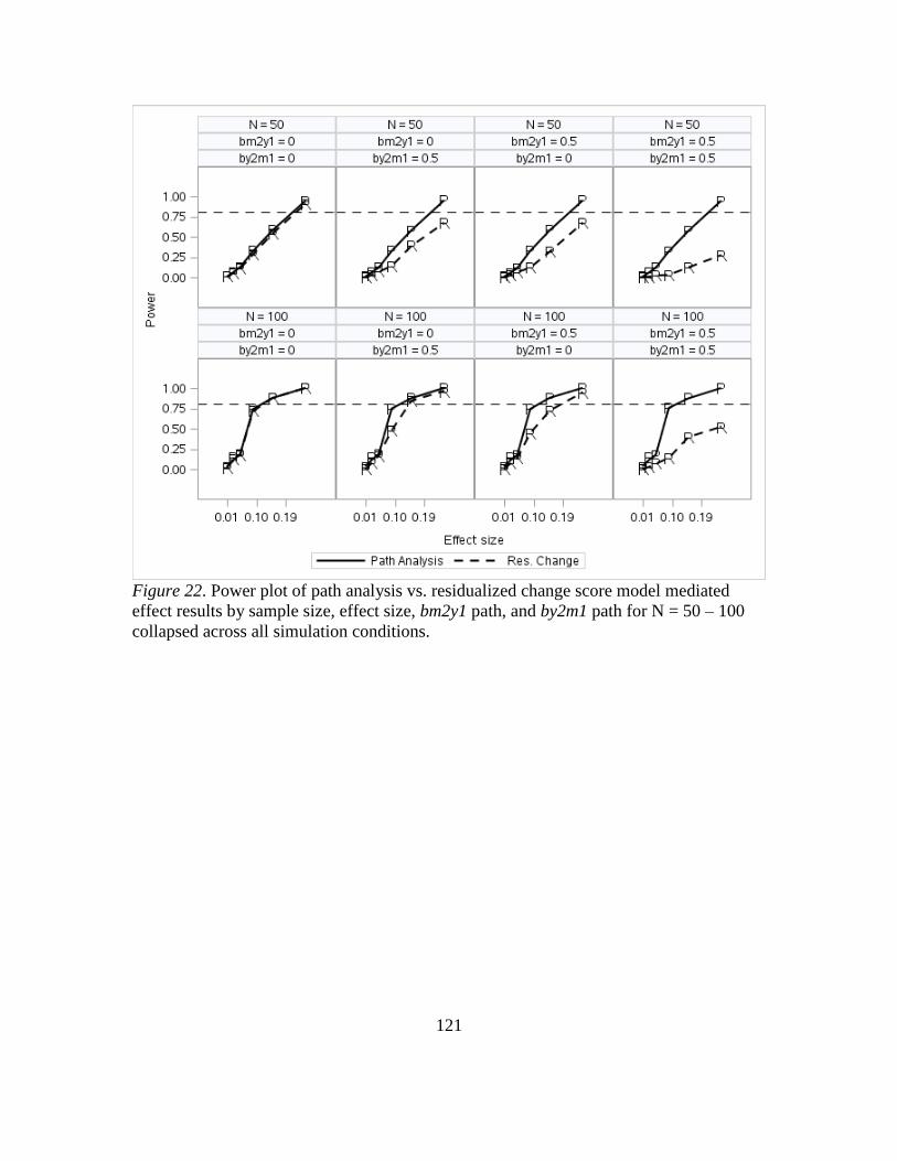
121
Figure 22. Power plot of path analysis vs. residualized change score model mediated
effect results by sample size, effect size, bm2y1 path, and by2m1 path for N = 50 – 100
collapsed across all simulation conditions.
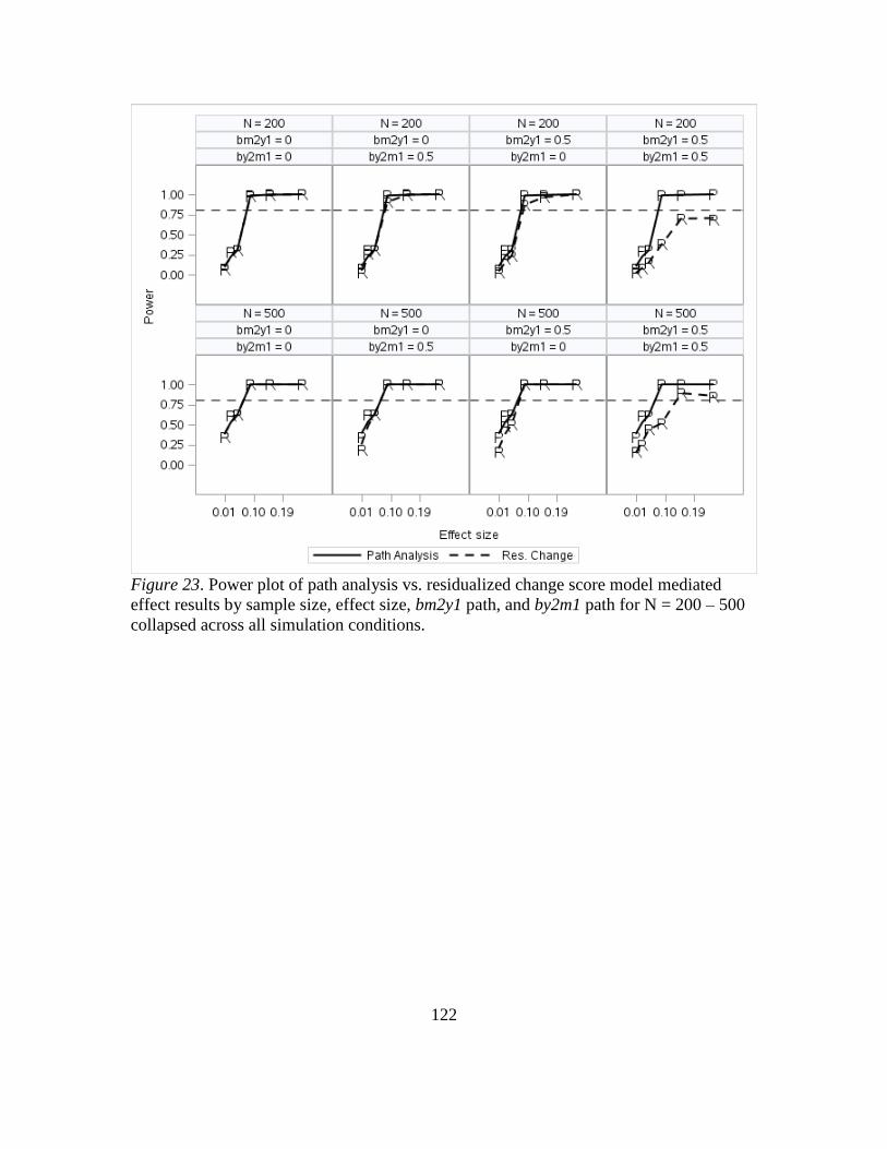
122
Figure 23. Power plot of path analysis vs. residualized change score model mediated
effect results by sample size, effect size, bm2y1 path, and by2m1 path for N = 200 – 500
collapsed across all simulation conditions.
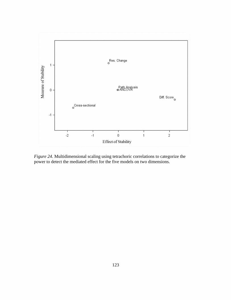
123
Figure 24. Multidimensional scaling using tetrachoric correlations to categorize the
power to detect the mediated effect for the five models on two dimensions.

124
APPENDIX A
LIST OF VARIABLE NAMES AND DESCRIPTIONS

125
Variable Description
X Treatment
M1 Pretest Mediator
Y1 Pretest Outcome
M2 Posttest Mediator
Y2 Posttest Outcome
ΔM Mediator difference score
ΔY Outcome difference score
RM Mediator residualized change
score
RY Outcome residualized change
score

126
APPENDIX B
LIST OF MODEL COEFFICIENTS AND DESCRIPTIONS

127
Coefficient Description
am2x Effect of treatment X on posttest
mediator M2 adjusting for M1 and Y1
Sm2m1 Pooled within-group stability of
mediator
Sm2m1total Stability of mediator ignoring group
information
bm2y1 Effect of pretest outcome Y1 on posttest
mediator M2 adjusting for X and M1
c’y2x Effect of treatment X on posttest
outcome Y2 adjusting for Y1, Y2, and M2
Sy2y1 Pooled within-group stability of outcome
Sy2y1total Stability of outcome ignoring group
information
by2m1 Effect of pretest mediator M1 on the
posttest outcome Y2 adjusting for X, Y1,
and M2
by2m2 Effect of posttest mediator M2 on posttest
outcome Y2 adjusting for X, Y1,and M1
by1m1 Effect of pretest mediator M1 on pretest
outcome Y1
aΔ Effect of treatment X on the mediator
difference score
bΔ Effect of the mediator difference score
on the outcome difference score
adjusting for X
c’Δ Effect of the treatment X on the outcome
difference score adjusting for mediator
difference score
aR Effect of treatment X on the mediator
residualized change score
bR Effect of the mediator residualized
change score on the outcome
residualized change score adjusting for X
c’R Effect of the treatment X on the outcome
residualized change score adjusting for
mediator residualized change score
Note. by1m1 appears in the data generating model figure but was simulated to be
equivalent to a pretest correlation between the mediator and the outcome.

128
APPENDIX C
SAS MACRO FOR DATA-GENERATION

129
libname DATAGEN "F:\ASU\Sims\";
TITLE 'DATA GENERATION OF TWO-WAVE MEDIATION';
OPTIONS PS=59 LS=80 REPLACE NONOTES;
*The following two lines of code stop the SAS log
from being saved over iterations of the macro program;
FILENAME NULLOG DUMMY 'C:\NULL';
PROC PRINTTO LOG=NULLOG;
PROC DATASETS LIBRARY=WORK KILL NOLIST; RUN;
%MACRO simulate(nsim,nobs,BMX,BYX,BYM,
aM1X,sm2m1,am2x,bm2y1,
by1m1,cy1x,cy2x,sy2y1,
by2m1,by2m2,varx,varm1,
varm2,vary1,vary2,RELM1,
RELM2, RELY1, RELY2,file,
TYPE,ERROR);
TITLE 'SIMULATION OF TWO-WAVE MEDIATION';
DATA DATAGEN.&FILE;
totaln=&NSIM*&NOBS;
DO I=1 TO totaln;
/*variances and covariances for relability - Reliability will not be
varied in this simulation!*/
VarX=0.25;
VarM1=(&aM1X**2)*VarX+(&VarM1)**2;
CovXM1=&aM1X*VarX;
CovXY1=&cY1X*VarX+&bY1M1*CovXM1;
CovXM2=&aM2X*VarX+&sM2M1*CovXM1+&bM2Y1*CovXY1;
CovXY2=&cY2X*VarX+&SY2Y1*CovXY1+&bY2M1*CovXM1+&bY2M2*CovXM2;
CovM1Y1=&aM1X*&cY1X*VarX+&aM1X*&bY1M1*CovXM1+&bY1M1*&VarM1**2;
CovM1M2=&aM1X*&SM2M1*CovXM1+&aM1X*&bM2Y1*CovXY1+&aM1X*&aM2X*VarX+&SM2M1
*&VarM1+&bM2Y1*&bY1M1*&VarM1**2;
CovM1Y2=&aM1X*&cY2X*VarX+&aM1X*&SY2Y1*CovXY1+&aM1X*&bY2M1*CovXM1+&aM1X*
&bY2M2*CovXM2+&SY2Y1*&bY1M1*&VarM1**2+&bY2M1*&VarM1**2+&bY2M2*&SM2M1*&V
arM1**2+&bY2M2*&bM2Y1*&bY1M1*&VarM1**2;
CovM2Y1=&aM2X*&bY1M1*CovXM1+&aM2X*&cY1X*VarX+&SM2M1*&bY1M1*VarM1+&SM2M1
*&cY1X*CovXM1+&bM2Y1*&bY1M1*CovM1Y1+&bM2Y1*&cY1X*CovXY1+&bM2Y1*(&VarY1)
**2;
VarY1=(&cY1X**2)*VarX+2*&cY1X*&bY1M1*CovXM1+(&bY1M1**2)*VarM1+(&VarY1)*
*2;
VarM2=(&SM2M1**2)*VarM1+2*&SM2M1*&bM2Y1*CovM1Y1+2*&SM2M1*&aM2X*CovXM1+(
&bM2Y1**2)*VarY1+2*&bM2Y1*&aM2X*CovXY1+(&aM2X**2)*VarX+(&VarM2)**2;
VarY2=(&cY2X**2)*VarX+2*&cY2X*&SY2Y1*CovXY1+2*&cY2X*&bY2M1*CovXM1+2*&cY
2X*&bY2M2*CovXM2+(&SY2Y1**2)*VarY1+2*&SY2Y1*&bY2M1*CovM1Y1+2*&SY2Y1*&bY
2M2*CovM2Y1+
(&bY2M1**2)*VarM1+2*&bY2M1*&bY2M2*CovM1M2+(&bY2M2**2)*VarM2+(&VarY2)**2
;

130
CovM2Y2=&SM2M1*&cY2X*CovXM1+&SM2M1*&SY2Y1*CovM1Y1+&SM2M1*&bY2M1*VarM1+&
SM2M1*&bY2M2*CovM1M2+&bM2Y1*&cY2X*CovXY1+&bM2Y1*&SY2Y1*VarY1+&bM2Y1*&bY
2M1*CovM1Y1+
&bM2Y1*&bY2M2*CovM2Y1+&aM2X*&cY2X*VarX+&aM2X*&SY2Y1*CovXY1+&aM2X*&bY2M1
*CovXM1+&aM2X*&bY2M2*CovXM2+&bY2M2*(&VarM2)**2;
CovY1Y2=&cY1X*&SY2Y1*CovXY1+&cY1X*&bY2M1*CovXM1+&cY1X*&bY2M2*CovXM2+&cY
1X*&cY2X*VarX+&bY1M1*&SY2Y1*CovM1Y1+&bY1M1*&bY2M1*VarM1+&bY2M2*&bY1M1*C
ovM1M2+
&bY1M1*&cY2X*CovXM1+&bY2M2*&bM2Y1*(&VarY1)**2+&SY2Y1*(&VarY1)**2;
/*model variables*/
X=&varx*rannor(0); IF X LT 0 THEN X=0; IF X GT 0 THEN X=1;
M1t=&varm1*rannor(0);
Varm1e=(Varm1/&RELM1)-Varm1;
M1e=sqrt(varm1e)*rannor(0);
M1=m1t+m1e;
M2T=&bm2y1*y1+&sm2m1*m1+&am2x*x+&varm2*rannor(0);
VarM2e=(VarM2/&RELM2)-VarM2;
M2e=sqrt(varm2e)*rannor(0);
M2=M2T+M2e;
Y1T=&by1m1*m1+&vary1*rannor(0);
Vary1e=(vary1/&RELY1)-vary1;
Y1e=sqrt(vary1e)*rannor(0);
Y1=Y1T+Y1e;
Y2T=&cy2x*x+&sy2y1*y1+&by2m1*m1+&by2m2*m2+&vary2*rannor(0);
Vary2e=(Vary2/&RELY2)-Vary2;
Y2e=sqrt(vary2e)*rannor(0);
Y2=Y2T+y2e;
Mdiff=M2-M1;
Ydiff=Y2-Y1;
OUTPUT;
END;
drop y1e y1t m1e m1t y2e y2t m2e m2t vary1e varm1e vary2e varm2e;
run;
%END;
%MEND;
run;
PROC DATASETS LIB=WORK NOLIST;
%simulate(nsim=10,nobs=200,BMX=0,BYX=0,BYM=0,
aM1X=0, sm2m1=.981,am2x=0,bm2y1=0, by1m1=.578,
cy1x=0, cy2x=0,sy2y1=.686, by2m1=.876,by2m2=0,
varx=1,varm1=1,varm2=1,vary1=1,vary2=1,
RELM1=1, RELM2=1, RELY1=1, RELY2=1,
FILE=n200cond1,TYPE='CCC',ERROR=1);
run; quit;

131
APPENDIX D
FIGURE OF DATA-GENERATING MODEL

132

133
APPENDIX E
ESTIMATED QUANTITIES AND MODEL CONDITIONS

134
Conditions
Model Quantity
Estimated
Stability M – Y
Cross-lag
Y – M
Cross-lag
Pretest
correlation
ANCOVA am2x *by2m2 Equal across
groups
None None None
Path analysis am2x *by2m2 Equal across
groups
None None None
Difference
Score
aΔ *bΔ Equal to 1 None None None
Residualized
Change score
aR *bR Equal across
groups
Equals 0 Equals 0 Equals 0
Cross-
sectional
am2x *by2m2 Equals 0 Equals 0 Equals 0 Equals 0
Note. The mediated effect estimated with the cross-sectional model consists of the same
path coefficients as the ANCOVA/path analysis model but ignores all pretest information
on M and Y when estimating these quantities.

135
APPENDIX F
SAS MACRO FOR ANALYSIS OF ALL MODELS

136
libname DATAGEN "E:\ASU\Sims\Two-wave model\Valente Masters
Sim\DATAGEN\";
libname DATAOUT "E:\ASU\Sims\Two-wave model\Valente Masters
Sim\DATAOUT";
FILENAME NULLOG DUMMY 'D:\NULL';
PROC PRINTTO LOG=NULLOG;
PROC DATASETS LIBRARY=WORK KILL NOLIST; RUN;
%MACRO ANALYZE (nsim,nobs,BMX,BYX,BYM,
aM1X,sm2m1,am2x,bm2y1,
by1m1,cy1x,cy2x,sy2y1,
by2m1,by2m2,varx,varm1,
varm2,vary1,vary2,RELM1,
RELM2, RELY1, RELY2,file,
TYPE,ERROR);
DATA SIM; SET DATAGEN.&FILE;
J=&nobs;
DO J=0 to totaln by &nobs;
IF 1+J<=I<=&NOBS+J then rep=1+(J/&nobs);
end;
run;
/***************************************************************/
/* */
/* PATH MODEL */
/* */
/***************************************************************/
PROC CALIS DATA=SIM METHOD=ML NORPINT PLC OUTEST=OUT1 outstat=out2;
by rep;
LINEQS
M2=sm2m1_ M1 + am2x_ X + bm2y1_ Y1+ E2,
y2=cy2x_ X + sy2y1_ y1 + by2m1_ M1 + by2m2_ M2 + E3;
Cov
X M1,
X Y1,
M1 Y1;
STD
E2 = EE2,
E3 = EE3;
RUN;
*SAVING THE PARAMETER VALUES OF FROM THE PATH MODEL OUTPUT. PARAMETERS
ARE DENOTED WITH _ AT THE END OF THE NAME;
DATA CALPARMS; SET OUT1;
IF _TYPE_="PARMS";
KEEP sM2M1_ aM2X_ cY2X_ sY2Y1_ bY2M1_ bY2M2_;
run;
*SAVING THE STANDARD ERRORS OF THE PARAMETERS FROM THE PATH MODEL
OUTPUT;
DATA CALSTDERR1; SET OUT1;

137
IF _TYPE_="STDERR"; SEsM2M1_= sM2M1_;
KEEP SEsM2M1_;
DATA CALSTDERR2; SET OUT1;
IF _TYPE_="STDERR"; SEaM2X_= aM2X_;
KEEP SEaM2X_;
DATA CALSTDERR3; SET OUT1;
IF _TYPE_="STDERR"; SEcY2X_= cY2X_;
KEEP SEcY2X_;
DATA CALSTDERR4; SET OUT1;
IF _TYPE_="STDERR"; SEsY2Y1_= sY2Y1_;
KEEP SEsY2Y1_;
DATA CALSTDERR5; SET OUT1;
IF _TYPE_="STDERR"; SEbY2M1_= bY2M1_;
KEEP SEbY2M1_;
DATA CALSTDERR6; SET OUT1;
IF _TYPE_="STDERR"; SEbY2M2_= bY2M2_;
KEEP SEbY2M2_;
*MERGING THE STANDARD ERROR DATA SETS FOR EACH PARAMETER VALUE INTO ONE
DATASET;
DATA CALSTDERR; MERGE CALSTDERR1 CALSTDERR2 CALSTDERR3 CALSTDERR4
CALSTDERR5 CALSTDERR6;
RUN;
*SAVING THE COVARIANCES AND VARIANCES OF THE VARIABLES FROM THE PATH
MODEL OUTPUT. COVARIANCES DENOTED CV AND VARIANCES DENOTED VARI;
DATA CALISAA; SET OUT2;
IF _TYPE_="COV";IF _NAME_= "M1";CVXM1= X;
KEEP CVXM1;
DATA CALISAB; SET OUT2;
IF _TYPE_="COV";IF _NAME_= "M2";CVXM2= X;
KEEP CVXM2;
DATA CALISAC; SET OUT2;
IF _TYPE_="COV";IF _NAME_= "Y1";CVXy1= X;
KEEP CVXy1;
DATA CALISAD; SET OUT2;
IF _TYPE_="COV";IF _NAME_= "Y2";CVXY2= X;
KEEP CVXY2;
DATA CALISAE; SET OUT2;
IF _TYPE_="COV"; IF _NAME_='M1'; CVM1M2=M2;
KEEP CVM1M2;
DATA CALISAF; SET OUT2;
IF _TYPE_="COV"; IF _NAME_='M1'; CVM1Y1=y1;
KEEP CVM1Y1;
DATA CALISAG; SET OUT2;
IF _TYPE_="COV"; IF _NAME_='M1'; CVM1Y2=Y2;
KEEP CVM1Y2;
DATA CALISAH; SET OUT2;
IF _TYPE_="COV"; IF _NAME_='M2'; CVM2Y1=y1;
KEEP CVM2Y1;
DATA CALISAI; SET OUT2;
IF _TYPE_="COV"; IF _NAME_='M2'; CVM2Y2=Y2;
KEEP CVM2Y2;
DATA CALISAJ; SET OUT2;

138
IF _TYPE_="COV"; IF _NAME_='Y1'; CVY1Y2=Y2;
KEEP CVY1Y2;
DATA CALISAK; SET OUT2;
IF _TYPE_='COV'; IF _NAME_="X"; VARIX=X;
KEEP VARIX;
DATA CALISAL; SET OUT2;
IF _TYPE_='COV'; IF _NAME_="M1"; VARIM1=M1;
KEEP VARIM1;
DATA CALISAM; SET OUT2;
IF _TYPE_='COV'; IF _NAME_="M2"; VARIM2=M2;
KEEP VARIM2;
DATA CALISAN; SET OUT2;
IF _TYPE_='COV'; IF _NAME_="Y1"; VARIY1=y1;
KEEP VARIY1;
DATA CALISAO; SET OUT2;
IF _TYPE_='COV'; IF _NAME_="Y2"; VARIY2=Y2;
KEEP VARIY2;
*MERGING THE COVARIANCES AND VARIANCES OF THE VARIABLES FROM THE PATH
MODEL OUTPUT INTO ONE DATASET;
DATA CALCOV; MERGE CALISAA CALISAB CALISAC CALISAD CALISAE CALISAF
CALISAG CALISAH CALISAI CALISAJ
CALISAK CALISAL CALISAM CALISAN CALISAO;
RUN;
*COMPUTES CORRELATIONS BASED ON PATH MODEL OUTPUT;
DATA CALCORR; SET CALCOV;
CRXM1=CVXM1/(SQRT(VARIX)*SQRT(VARIM1));
CRXM2=CVXM2/(SQRT(VARIX)*SQRT(VARIM2));
CRXY1=CVXY1/(SQRT(VARIX)*SQRT(VARIY1));
CRXY2=CVXY2/(SQRT(VARIX)*SQRT(VARIY2));
CRM1M2=CVM1M2/(SQRT(VARIM1)*SQRT(VARIM2));
CRM1Y1=CVM1Y1/(SQRT(VARIM1)*SQRT(VARIY1));
CRM1Y2=CVM1Y2/(SQRT(VARIM1)*SQRT(VARIY2));
CRM2Y1=CVM2Y1/(SQRT(VARIM2)*SQRT(VARIY1));
CRM2Y2=CVM2Y2/(SQRT(VARIM2)*SQRT(VARIY2));
CRY1Y2=CVY1Y2/(SQRT(VARIY1)*SQRT(VARIY2));
RUN;
*THIS MERGES ALL THE OUTPUT FROM THE PATH MODEL OUTPUT INTO ONE
DATASET;
DATA CALIS; MERGE CALPARMS CALSTDERR CALCORR;
/***************************************************************/
/* */
/* CHANGE SCORES */
/* */
/***************************************************************/
/*ESTIMATING (DIFFM=X Y1) REGRESSION AND SAVING THE VALUES OF THE
COEFFICIENTS AND THEIR STANDARD ERRORS*/
PROC REG DATA=SIM OUTEST=DiffFILE1 COVOUT noprint; by rep; MODEL Mdiff=
X/;
DATA DiffA; SET DiffFILE1; IF _TYPE_='PARMS'; aM2XDiff=X;
MSEAM2XDiff=_RMSE_*_RMSE_;

139
DROP _MODEL_ _NAME_ _TYPE_ _DEPVAR_ _RMSE_ INTERCEP X;
KEEP aM2XDiff MSEAM2XDiff;
DATA DiffB; SET DiffFILE1;IF _NAME_='X'; SEAM2XDiff=SQRT(X);
DROP _MODEL_ _NAME_ _TYPE_ _DEPVAR_ _RMSE_ INTERCEP X;
KEEP SEAM2XDiff;
DATA DiffMODEL1; MERGE DiffA DIffB;
*Estimating the (DiffY=X DiffM) REGRESSION AND SAVING THE VALUES OF THE
COEFFICIENTS AND THEIR STANDARD ERRORS;
PROC REG DATA=SIM OUTEST=DiffFILE2 COVOUT noprint; by rep; MODEL
Ydiff=X Mdiff/;
DATA DiffE; SET DiffFILE2;IF _TYPE_='PARMS'; cY2XDiff=X;
MSECY2XDiff=_RMSE_*_RMSE_;
DROP _MODEL_ _NAME_ _TYPE_ _DEPVAR_ _RMSE_ INTERCEP X MDiff;
KEEP cY2Xdiff MSECY2Xdiff;
DATA DiffF; SET DiffFILE2;IF _NAME_='X'; SECY2XDiff=SQRT(X);
DROP _MODEL_ _NAME_ _TYPE_ _DEPVAR_ _RMSE_ INTERCEP X MDiff;
KEEP SECY2XDiff;
DATA DiffG; SET DiffFILE2;IF _TYPE_='PARMS'; bY2M2Diff=Mdiff;
MSEBY2M2DIff=_RMSE_*_RMSE_;
DROP _MODEL_ _NAME_ _TYPE_ _DEPVAR_ _RMSE_ INTERCEP X MDiff;
KEEP bY2M2Diff MSEBY2M2Diff;
DATA DiffH; SET DiffFILE2;IF _NAME_='Mdiff'; SEBY2M2Diff=SQRT(Mdiff);
DROP _MODEL_ _NAME_ _TYPE_ _DEPVAR_ _RMSE_ INTERCEP X MDiff;
KEEP SEBY2M2Diff;
DATA DiffMODEL2; MERGE DiffE DiffF DiffG DiffH;
DATA DiffMODELS; MERGE DiffMODEL1 DiffMODEL2;
/***************************************************************/
/* */
/* RESIDUALIZED CHANGE SCORES */
/* */
/***************************************************************/
/*MODEL COMPUTING AND SAVING RESIDUALIZED DIFFERENCE SCORE OF M1 AND
M2*/
PROC REG DATA=SIM noprint; by rep; MODEL M2=M1/;
output out=resid1 r=residm;
data rchange1;set resid1;
keep residm x;
/*MODEL COMPUTING AND SAVING RESIDUALIZED DIFFERENCE SCORE OF Y1 AND
Y2*/
PROC REG DATA=SIM noprint; by rep; MODEL Y2=y1/;
output out=resid2 r=residy;
data rchange2;set resid2;
keep residy;
proc sort; by I;
data rchange; merge resid1 resid2; by I;
/*ESTIMATING (RESIDM2=X Y1) REGRESSION AND SAVING THE VALUES OF THE
COEFFICIENTS AND THEIR STANDARD ERRORS*/

140
PROC REG DATA=rchange OUTEST=RFILE1 COVOUT noprint; by rep; MODEL
residm= X/;
DATA RA; SET RFILE1; IF _TYPE_='PARMS'; aM2XRES=X;
MSEAM2XRES=_RMSE_*_RMSE_;
DROP _MODEL_ _NAME_ _TYPE_ _DEPVAR_ _RMSE_ INTERCEP X;
KEEP aM2XRES MSEAM2XRES;
DATA RB; SET RFILE1;IF _NAME_='X'; SEAM2XRES=SQRT(X);
DROP _MODEL_ _NAME_ _TYPE_ _DEPVAR_ _RMSE_ INTERCEP X;
KEEP SEAM2XRES;
DATA RESMODEL1; MERGE RA RB;
*Estimating the (RESIDY2=X RESIDM2) REGRESSION AND SAVING THE VALUES OF
THE COEFFICIENTS AND THEIR STANDARD ERRORS;
PROC REG DATA=rchange OUTEST=RFILE2 COVOUT noprint; by rep; MODEL
RESIDY=X RESIDM/;
DATA RE; SET RFILE2;IF _TYPE_='PARMS'; cY2XRES=X;
MSECY2XRES=_RMSE_*_RMSE_;
DROP _MODEL_ _NAME_ _TYPE_ _DEPVAR_ _RMSE_ INTERCEP X RESIDM;
KEEP cY2XRES MSECY2XRES;
DATA RF; SET RFILE2;IF _NAME_='X'; SECY2XRES=SQRT(X);
DROP _MODEL_ _NAME_ _TYPE_ _DEPVAR_ _RMSE_ INTERCEP X RESIDM;
KEEP SECY2XRES;
DATA RG; SET RFILE2;IF _TYPE_='PARMS';
bY2M2RES=RESIDM;MSEBY2M2RES=_RMSE_*_RMSE_;
DROP _MODEL_ _NAME_ _TYPE_ _DEPVAR_ _RMSE_ INTERCEP X RESIDM;
KEEP bY2M2RES MSEBY2M2RES;
DATA RH; SET RFILE2;IF _NAME_='residm'; SEBY2M2RES=SQRT(residm);
DROP _MODEL_ _NAME_ _TYPE_ _DEPVAR_ _RMSE_ INTERCEP X RESIDM;
KEEP SEBY2M2RES;
DATA RESMODEL2; MERGE RE RF RG RH;
DATA RESMODELS; MERGE RESMODEL1 RESMODEL2;
/***************************************************************/
/* */
/* LINEAR REGRESSION (ANCOVA) */
/* */
/***************************************************************/
*Estimating the (M1=X) regression and saving the value of aM1X and its
standard error;
/*PROC REG DATA=SIM OUTEST=FILE1 COVOUT noprint; MODEL M1=X/;
DATA B; SET FILE1;IF _TYPE_='PARMS'; aM1X=X; MSEM1X=_RMSE_*_RMSE_;
DROP _MODEL_ _NAME_ _TYPE_ _DEPVAR_ _RMSE_ INTERCEP X M1;
KEEP aM1X MSEM1X;
DATA C; SET FILE1;IF _NAME_='X'; SEAM1X=SQRT(X);
DROP _MODEL_ _NAME_ _TYPE_ _DEPVAR_ _RMSE_ INTERCEP X M1;
KEEP SEAM1X;
DATA MODEL1; MERGE B C; */
*Estimating the (M2=M1 X) regression and saving the value of sM2M1,
aM2X, and their standard errors;
PROC REG DATA=SIM OUTEST=FILE2 COVOUT noprint; by rep; MODEL M2=M1 Y1
X/;

141
DATA D; SET FILE2;IF _TYPE_='PARMS'; sM2M1=M1; MSEM2M1=_RMSE_*_RMSE_;
DROP _MODEL_ _NAME_ _TYPE_ _DEPVAR_ _RMSE_ INTERCEP X M1 M2;
KEEP sM2M1 MSEM2M1;
DATA E; SET FILE2;IF _NAME_='M1'; SESM2M1=SQRT(M1);
DROP _MODEL_ _NAME_ _TYPE_ _DEPVAR_ _RMSE_ INTERCEP X M1 M2;
KEEP SESM2M1;
DATA F; SET FILE2; IF _TYPE_='PARMS'; aM2X=X;MSEAM2X=_RMSE_*_RMSE_;
DROP _MODEL_ _NAME_ _TYPE_ _DEPVAR_ _RMSE_ INTERCEP X M1 M2;
KEEP aM2X MSEAM2X;
DATA G; SET FILE2;IF _NAME_='X'; SEAM2X=SQRT(X);
DROP _MODEL_ _NAME_ _TYPE_ _DEPVAR_ _RMSE_ INTERCEP X M1 M2;
KEEP SEAM2X;
DATA H; SET FILE2; IF _TYPE_='PARMS'; bM2Y1=Y1;MSEBM2Y1=_RMSE_*_RMSE_;
DROP _MODEL_ _NAME_ _TYPE_ _DEPVAR_ _RMSE_ INTERCEP X Y1 M1 M2;
KEEP bM2Y1 MSEBM2Y1;
DATA I; SET FILE2; IF _NAME_='y1'; SEBM2Y1=SQRT(y1);
DROP _MODEL_ _NAME_ _TYPE_ _DEPVAR_ _RMSE_ INTERCEP X Y1 M1 M2;
KEEP SEBM2Y1;
DATA MODEL2; MERGE D E F G H I;
*Estimating the (Y1=M1) regression and saving the value of bY1M1 and
its standard errors;
PROC REG DATA=SIM OUTEST=FILE3 COVOUT noprint; by rep; MODEL Y1=M1/;
DATA J; SET FILE3;IF _TYPE_='PARMS'; bY1M1=M1;MSEBY1M1=_RMSE_*_RMSE_;
DROP _MODEL_ _NAME_ _TYPE_ _DEPVAR_ _RMSE_ INTERCEP M1 Y1;
KEEP bY1M1 MSEBY1M1;
DATA K; SET FILE3;IF _NAME_='M1'; SEBY1M1=SQRT(M1);
DROP _MODEL_ _NAME_ _TYPE_ _DEPVAR_ _RMSE_ INTERCEP M1 Y1;
KEEP SEBY1M1;
/*DATA L; SET FILE3;IF _TYPE_='PARMS'; cY1X=X;MSECY1X=_RMSE_*_RMSE_;
DROP _MODEL_ _NAME_ _TYPE_ _DEPVAR_ _RMSE_ INTERCEP X M1 Y1;
KEEP cY1X MSECY1X;
DATA M; SET FILE3;IF _NAME_='X'; SECY1X=SQRT(X);
DROP _MODEL_ _NAME_ _TYPE_ _DEPVAR_ _RMSE_ INTERCEP X M1 Y1;
KEEP SECY1X;*/
DATA MODEL3; MERGE J K;
*Estimating the (Y2=X Y1 M1 M2) regression and saving the value of
sM2M1, aM2X, bM2Y1, and their standard errors;
PROC REG DATA=SIM OUTEST=FILE4 COVOUT noprint; by rep; MODEL Y2=X Y1 M1
M2/;
DATA N; SET FILE4;IF _TYPE_='PARMS'; cY2X=X;MSECY2X=_RMSE_*_RMSE_;
DROP _MODEL_ _NAME_ _TYPE_ _DEPVAR_ _RMSE_ INTERCEP X Y1 Y2 M1 M2;
KEEP cY2X MSECY2X;
DATA O; SET FILE4;IF _NAME_='X'; SECY2X=SQRT(X);
DROP _MODEL_ _NAME_ _TYPE_ _DEPVAR_ _RMSE_ INTERCEP X Y1 Y2 M1 M2;
KEEP SECY2X;
DATA P; SET FILE4;IF _TYPE_='PARMS'; sY2Y1=Y1;MSESY2Y1=_RMSE_*_RMSE_;
DROP _MODEL_ _NAME_ _TYPE_ _DEPVAR_ _RMSE_ INTERCEP X Y1 M1 M2;
KEEP sY2Y1 MSESY2Y1;
DATA Q; SET FILE4;IF _NAME_='Y1'; SESY2Y1=SQRT(Y1);
DROP _MODEL_ _NAME_ _TYPE_ _DEPVAR_ _RMSE_ INTERCEP X Y1 M1 M2;
KEEP SESY2Y1;
DATA R; SET FILE4;IF _TYPE_='PARMS'; bY2M1=M1;MSEBY2M1=_RMSE_*_RMSE_;

142
DROP _MODEL_ _NAME_ _TYPE_ _DEPVAR_ _RMSE_ INTERCEP X Y1 M1 M2;
KEEP bY2M1 MSEBY2M1;
DATA S; SET FILE4;IF _NAME_='M1'; SEBY2M1=SQRT(M1);
DROP _MODEL_ _NAME_ _TYPE_ _DEPVAR_ _RMSE_ INTERCEP X Y1 M1 M2;
KEEP SEBY2M1;
DATA T; SET FILE4;IF _TYPE_='PARMS'; bY2M2=M2;MSEBY2M2=_RMSE_*_RMSE_;
DROP _MODEL_ _NAME_ _TYPE_ _DEPVAR_ _RMSE_ INTERCEP X Y1 M1 M2;
KEEP bY2M2 MSEBY2M2;
DATA U; SET FILE4;IF _NAME_='M2'; SEBY2M2=SQRT(M2);
DROP _MODEL_ _NAME_ _TYPE_ _DEPVAR_ _RMSE_ INTERCEP X Y1 M1 M2;
KEEP SEBY2M2;
DATA MODEL4; MERGE N O P Q R S T U;
/*Estimating various total effect of X on Y2 IN PROGRESS
PROC REG DATA=SIM OUTEST-FILE5 COVOUT noprint; MODEL Y2=X/;
DATA V; SET FILE5L IF _TYPE_='PARMS'; CX=X; MSECX=_RMSE_*_RMSE_;
DROP _MODEL_ _NAME_ _TYPE_ _DEPVAR_ _RMSE_ INTERCEP X Y2;
KEEP CX MSECX;
PROC REG DATA=SIM OUTEST-FILE5 COVOUT noprint; MODEL Y2=X/;
DATA W; SET FILE5L IF _NAME_='X'; SECX=SQRT(X);
DROP _MODEL_ _NAME_ _TYPE_ _DEPVAR_ _RMSE_ INTERCEP X Y2;
KEEP SECX;
MODEL5; MERGE V W;*/
/***************************************************************/
/* */
/* CROSS SECTIONAL MEDIATOR MODEL */
/* */
/***************************************************************/
*Estimating the (M2=X) regression and saving the value of a and its
standard error;
PROC REG DATA=SIM OUTEST=FILE5 COVOUT noprint; by rep; MODEL M2= X/;
DATA V; SET FILE5; IF _TYPE_='PARMS'; a=X;MSEA=_RMSE_*_RMSE_;
DROP _MODEL_ _NAME_ _TYPE_ _DEPVAR_ _RMSE_ INTERCEP X M2;
KEEP a MSEA;
DATA W; SET FILE5;IF _NAME_='X'; SEA=SQRT(X);
DROP _MODEL_ _NAME_ _TYPE_ _DEPVAR_ _RMSE_ INTERCEP X M2;
KEEP SEA;
DATA MODEL5; MERGE V W;
*Estimating the (Y2=X M2) regression and saving the value of c b and
their standard errors;
PROC REG DATA=SIM OUTEST=FILE6 COVOUT noprint; by rep; MODEL Y2=X M2/;
DATA X; SET FILE6;IF _TYPE_='PARMS'; c=X; MSEC=_RMSE_*_RMSE_;
DROP _MODEL_ _NAME_ _TYPE_ _DEPVAR_ _RMSE_ INTERCEP X Y2 M2;
KEEP c MSEC;
DATA Y; SET FILE6;IF _NAME_='X'; SEC=SQRT(X);
DROP _MODEL_ _NAME_ _TYPE_ _DEPVAR_ _RMSE_ INTERCEP X Y2 M2;
KEEP SEC;
DATA Z; SET FILE6;IF _TYPE_='PARMS'; b=M2;MSEB=_RMSE_*_RMSE_;
DROP _MODEL_ _NAME_ _TYPE_ _DEPVAR_ _RMSE_ INTERCEP X Y2 M2;
KEEP b MSEB;
DATA AA; SET FILE6;IF _NAME_='M2'; SEB=SQRT(M2);

143
DROP _MODEL_ _NAME_ _TYPE_ _DEPVAR_ _RMSE_ INTERCEP X Y2 M2;
KEEP SEB;
DATA MODEL6; MERGE X Y Z AA;
*THIS MERGES ALL THE PREVIOUS REGRESSION, CHANGE SCORE, RES CHANGE, AND
PATH MODEL OUTPUT;
DATA ALL; MERGE MODEL2 MODEL3 MODEL4 MODEL5 MODEL6 DIFFMODELS RESMODELS
CALIS;
RUN;
*THIS COMPUTES COVARIANCES OF VARIABLES VIA PROC CORR;
PROC CORR DATA=SIM cov nocorr OUTPUT=COV noprint; by rep;
var x m1 m2 y1 y2 YDIFF MDIFF;
DATA SA; SET COV;
IF _NAME_='M1'; COVXM1=X;
KEEP COVXM1;
DATA SB; SET COV;
IF _NAME_='M2'; COVXM2=X;
KEEP COVXM2;
DATA SC; SET COV;
IF _NAME_='Y1'; COVXY1=X;
KEEP COVXY1;
DATA SD; SET COV;
IF _NAME_='Y2'; COVXY2=X;
KEEP COVXY2;
DATA SE; SET COV;
IF _NAME_='M1'; COVM1M2=M2;
KEEP COVM1M2;
DATA SF; SET COV;
IF _NAME_='M1'; COVM1Y1=y1;
KEEP COVM1Y1;
DATA SG; SET COV;
IF _NAME_='M1'; COVM1Y2=Y2;
KEEP COVM1Y2;
DATA SH; SET COV;
IF _NAME_='M2'; COVM2Y1=y1;
KEEP COVM2Y1;
DATA SI; SET COV;
IF _NAME_='M2'; COVM2Y2=Y2;
KEEP COVM2Y2;
DATA SJ; SET COV;
IF _NAME_='Y1'; COVY1Y2=Y2;
KEEP COVY1Y2;
DATA SK; SET COV;
IF _TYPE_='STD'; VAX=X*X;
KEEP VAX;
DATA SL; SET COV;
IF _TYPE_='STD'; VAM1=M1*M1;
KEEP VAM1;
DATA SM; SET COV;
IF _TYPE_='STD'; VAM2=M2*M2;

144
KEEP VAM2;
DATA SN; SET COV;
IF _TYPE_='STD'; VAY1=y1*y1;
KEEP VAY1;
DATA SO; SET COV;
IF _TYPE_='STD'; VAY2=Y2*Y2;
KEEP VAY2;
DATA SP; SET COV;
IF _TYPE_='STD'; VAYDIFF=YDIFF*YDIFF;
KEEP VAYDIFF;
DATA SQ; SET COV;
IF _TYPE_='STD'; VAMDIFF=MDIFF*MDIFF;
KEEP VAMDIFF;
DATA SR; SET COV;
IF _NAME_='Mdiff'; COVXMDIFF=X;
KEEP COVXMDIFF;
DATA SS; SET COV;
IF _NAME_='Ydiff'; COVXYDIFF=X;
KEEP COVXYDIFF;
DATA ST; SET COV;
IF _NAME_='Ydiff'; COVMDIFFYDIFF=Mdiff;
KEEP COVMDIFFYDIFF;
RUN;
PROC CORR DATA=rchange cov nocorr OUTPUT=COV2 noprint; by rep;
var X RESIDM RESIDY;
DATA SU; SET COV2;
IF _NAME_='residm'; COVXRESM=x;
KEEP COVXRESM;
DATA SV; SET COV2;
IF _NAME_='residy'; COVXRESY=x;
KEEP COVXRESY;
DATA SW; SET COV2;
IF _NAME_='residy'; COVRESMRESY=residm;
KEEP COVRESMRESY;
DATA SX; SET COV2;
IF _NAME_='residy'; VARESY=residy;
KEEP VARESY;
DATA SY; SET COV2;
IF _NAME_='residm'; VARESM=residm;
KEEP VARESM;
RUN;
*THIS MERGES ALL OF THE INDIVIDUAL COVARIANCE DATASETS INTO ONE
DATASET;
DATA SCOVS; MERGE SA SB SC SD SE SF SG SH SI SJ SK SL SM SN SO SP SQ SR
SS ST SU SV SW SX SY;
RUN;
*THIS COMPUTES THE CORRELATIONS FOR ALL THE VARIABLES VIA PROC CORR;
PROC CORR DATA=SIM OUTPUT=CORR noprint; by rep;
var x m1 m2 y1 y2;
DATA SAR; SET CORR;

145
IF _NAME_='M1'; CORRXM1=X;
KEEP CORRXM1;
DATA SBR; SET CORR;
IF _NAME_='M2'; CORRXM2=X;
KEEP CORRXM2;
DATA SCR; SET CORR;
IF _NAME_='Y1'; CORRXY1=x;
KEEP CORRXY1;
DATA SDR; SET CORR;
IF _NAME_='Y2'; CORRXY2=X;
KEEP CORRXY2;
DATA SER; SET CORR;
IF _NAME_='M1'; CORRM1M2=M2;
KEEP CORRM1M2;
DATA SFR; SET CORR;
IF _NAME_='M1'; CORRM1Y1=y1;
KEEP CORRM1Y1;
DATA SGR; SET CORR;
IF _NAME_='M1'; CORRM1Y2=Y2;
KEEP CORRM1Y2;
DATA SHR; SET CORR;
IF _NAME_='M2'; CORRM2Y1=y1;
KEEP CORRM2Y1;
DATA SIR; SET CORR;
IF _NAME_='M2'; CORRM2Y2=Y2;
KEEP CORRM2Y2;
DATA SJR; SET CORR;
IF _NAME_='Y1'; CORRY1Y2=y2;
KEEP CORRY1Y2;
RUN;
*THIS MERGES ALL THE INDIVIDUAL CORRELATION DATASETS INTO ONE DATASET;
DATA SCORRS; MERGE SAR SBR SCR SDR SER SFR SGR SHR SIR SJR;
RUN;
*P DENOTES POPULATION VALUE OF PARAMETER;
DATA TEST;SET ALL;
NSIM=&NSIM;
NOBS=&NOBS;
PaM1X=&aM1X;
PsM2M1=&sM2M1;
PaM2X=&aM2X;
PbM2Y1=&bM2Y1;
PbY1M1=&bY1M1;
PcY1X=&cY1X;
PcY2X=&cY2X;
PsY2Y1=&sY2Y1;
PbY2M1=&bY2M1;
PbY2M2=&bY2M2;
VARX=&VARX;
VARM1=&VARM1;
VARM2=&VARM2;
VARY1=&VARY1;
VARY2=&VARY2;

146
FILE=&FILE;
TYPE=&TYPE;
ERROR=&ERROR;
*The code below calculates the product of coefficients for all four
methods;
TRUEAB=PaM2X*PbY2M2;
AB=aM2X*bY2M2;
AB_=aM2X_*bY2M2_;
ABDIFF=aM2XDiff*bY2M2Diff;
ABRES=aM2XRES*bY2M2RES;
ABX=A*B;
*The code below computes the standard error for the product of the
coefficients for all four methods;
SEAB=SQRT((aM2X**2)*(SEbY2M2**2)+(bY2M2**2)*(SEaM2X**2));
SEAB_=SQRT((aM2X_**2)*(SEbY2M2_**2)+(bY2M2_**2)*(SEaM2X_**2));
SEABDIFF=SQRT((aM2XDiff**2)*(SEbY2M2Diff**2)+(bY2M2Diff**2)*(SEaM2XDiff
**2));
SEABRES=SQRT((aM2XRES**2)*(SEbY2M2RES**2)+(bY2M2RES**2)*(SEaM2XRES**2))
;
*The code below calculates empirical power of paths a, b, and c;
ZA=AM2X/SEAM2X;
PZA=1-PROBNORM(ABS(ZA));
SZA=0; IF PZA<=0.025 THEN SZA=1;
ZB=BY2M2/SEBY2M2;
PZB=1-PROBNORM(ABS(ZB));
SZB=0; IF PZB<=0.025 THEN SZB=1;
ZC=CY2X/SECY2X;
PZC=1-PROBNORM(ABS(ZC));
SZC=0; IF PZC<=0.025 THEN SZC=1;
ZADIFF=AM2XDIFF/SEAM2XDIFF;
PZADIFF=1-PROBNORM(ABS(ZADIFF));
SZADIFF=0; IF PZADIFF<=0.025 THEN SZADIFF=1;
ZBDIFF=BY2M2DIFF/SEBY2M2DIFF;
PZBDIFF=1-PROBNORM(ABS(ZBDIFF));
SZBDIFF=0; IF PZBDIFF<=0.025 THEN SZBDIFF=1;
ZCDIFF=CY2XDIFF/SECY2XDIFF;
PZCDIFF=1-PROBNORM(ABS(ZCDIFF));
SZCDIFF=0; IF PZCDIFF<=0.025 THEN SZCDIFF=1;
ZARES=AM2XRES/SEAM2XRES;
PZARES=1-PROBNORM(ABS(ZARES));
SZARES=0; IF PZARES<=0.025 THEN SZARES=1;
ZBRES=BY2M2RES/SEBY2M2RES;
PZBRES=1-PROBNORM(ABS(ZBRES));
SZBRES=0; IF PZBRES<=0.025 THEN SZBRES=1;

147
ZCRES=CY2XRES/SECY2XRES;
PZCRES=1-PROBNORM(ABS(ZCRES));
SZCRES=0; IF PZCRES<=0.025 THEN SZCRES=1;
ZA_=AM2X_/SEAM2X_;
PZA_=1-PROBNORM(ABS(ZA_));
SZA_=0; IF PZA_<=0.025 THEN SZA_=1;
ZB_=BY2M2_/SEBY2M2_;
PZB_=1-PROBNORM(ABS(ZB_));
SZB_=0; IF PZB_<=0.025 THEN SZB_=1;
ZC_=CY2X_/SECY2X_;
PZC_=1-PROBNORM(ABS(ZC_));
SZC_=0; IF PZC_<=0.025 THEN SZC_=1;
*The following code computes bias and relative bias for the four
methods (PATH MODEL, RES. CHANGE, CHANGE, ANCOVA(REGRESSION), AND CROSS
SECTIONAL MODEL);
BA=AM2X-PAM2X;
BAR=BA/PAM2X;
B2A=BA*BA;
BADIFF=AM2XDIFF-PAM2X;
BADIFFR=BADIFF/PAM2X;
B2ADIFF=BADIFF*BADIFF;
BARES=AM2XRES-PAM2X;
BARESR=BARES/PAM2X;
B2ARES=BARES*BARES;
BA_=AM2X_-PAM2X;
BA_R=BA_/PAM2X;
B2A_=BA_*BA_;
BAX=A-PAM2X;
BAXR=BAX/PAM2X;
B2AX=BAX*BAX;
BB=BY2M2-PBY2M2;
BBR=BB/PBY2M2;
B2B=BB*BB;
BBDIFF=BY2M2DIFF-PBY2M2;
BBDIFFR=BBDIFF/PBY2M2;
B2BDIFF=BBDIFF*BBDIFF;
BBRES=BY2M2RES-PBY2M2;
BBRESR=BBRES/PBY2M2;
B2BRES=BBRES*BBRES;
BB_=BY2M2_-PBY2M2;
BB_R=BB_/PBY2M2;
B2B_=BB_*BB_;
BBX=B-PBY2M2;
BBXR=BBX/PBY2M2;
B2BX=BBX*BBX;
BC=CY2X-PCY2X;
BCR=BC/PCY2X;
B2C=BC*BC;
SDBC=BC/SECY2X;
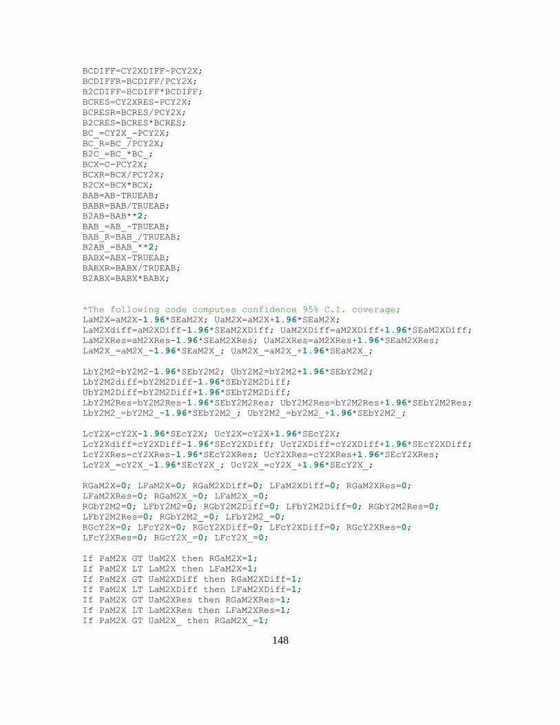
148
BCDIFF=CY2XDIFF-PCY2X;
BCDIFFR=BCDIFF/PCY2X;
B2CDIFF=BCDIFF*BCDIFF;
BCRES=CY2XRES-PCY2X;
BCRESR=BCRES/PCY2X;
B2CRES=BCRES*BCRES;
BC_=CY2X_-PCY2X;
BC_R=BC_/PCY2X;
B2C_=BC_*BC_;
BCX=C-PCY2X;
BCXR=BCX/PCY2X;
B2CX=BCX*BCX;
BAB=AB-TRUEAB;
BABR=BAB/TRUEAB;
B2AB=BAB**2;
BAB_=AB_-TRUEAB;
BAB_R=BAB_/TRUEAB;
B2AB_=BAB_**2;
BABX=ABX-TRUEAB;
BABXR=BABX/TRUEAB;
B2ABX=BABX*BABX;
*The following code computes confidence 95% C.I. coverage;
LaM2X=aM2X-1.96*SEaM2X; UaM2X=aM2X+1.96*SEaM2X;
LaM2Xdiff=aM2XDiff-1.96*SEaM2XDiff; UaM2XDiff=aM2XDiff+1.96*SEaM2XDiff;
LaM2XRes=aM2XRes-1.96*SEaM2XRes; UaM2XRes=aM2XRes+1.96*SEaM2XRes;
LaM2X_=aM2X_-1.96*SEaM2X_; UaM2X_=aM2X_+1.96*SEaM2X_;
LbY2M2=bY2M2-1.96*SEbY2M2; UbY2M2=bY2M2+1.96*SEbY2M2;
LbY2M2diff=bY2M2Diff-1.96*SEbY2M2Diff;
UbY2M2Diff=bY2M2Diff+1.96*SEbY2M2Diff;
LbY2M2Res=bY2M2Res-1.96*SEbY2M2Res; UbY2M2Res=bY2M2Res+1.96*SEbY2M2Res;
LbY2M2_=bY2M2_-1.96*SEbY2M2_; UbY2M2_=bY2M2_+1.96*SEbY2M2_;
LcY2X=cY2X-1.96*SEcY2X; UcY2X=cY2X+1.96*SEcY2X;
LcY2Xdiff=cY2XDiff-1.96*SEcY2XDiff; UcY2XDiff=cY2XDiff+1.96*SEcY2XDiff;
LcY2XRes=cY2XRes-1.96*SEcY2XRes; UcY2XRes=cY2XRes+1.96*SEcY2XRes;
LcY2X_=cY2X_-1.96*SEcY2X_; UcY2X_=cY2X_+1.96*SEcY2X_;
RGaM2X=0; LFaM2X=0; RGaM2XDiff=0; LFaM2XDiff=0; RGaM2XRes=0;
LFaM2XRes=0; RGaM2X_=0; LFaM2X_=0;
RGbY2M2=0; LFbY2M2=0; RGbY2M2Diff=0; LFbY2M2Diff=0; RGbY2M2Res=0;
LFbY2M2Res=0; RGbY2M2_=0; LFbY2M2_=0;
RGcY2X=0; LFcY2X=0; RGcY2XDiff=0; LFcY2XDiff=0; RGcY2XRes=0;
LFcY2XRes=0; RGcY2X_=0; LFcY2X_=0;
If PaM2X GT UaM2X then RGaM2X=1;
If PaM2X LT LaM2X then LFaM2X=1;
If PaM2X GT UaM2XDiff then RGaM2XDiff=1;
If PaM2X LT LaM2XDiff then LFaM2XDiff=1;
If PaM2X GT UaM2XRes then RGaM2XRes=1;
If PaM2X LT LaM2XRes then LFaM2XRes=1;
If PaM2X GT UaM2X_ then RGaM2X_=1;

149
If PaM2X LT LaM2X_ then LFaM2X_=1;
If PbY2M2 GT UbY2M2 then RGbY2M2=1;
If PbY2M2 LT LbY2M2 then LFbY2M2=1;
If PbY2M2 GT UbY2M2Diff then RGbY2M2Diff=1;
If PbY2M2 LT LbY2M2Diff then LFbY2M2Diff=1;
If PbY2M2 GT UbY2M2Res then RGbY2M2Res=1;
If PbY2M2 LT LbY2M2Res then LFbY2M2Res=1;
If PbY2M2 GT UbY2M2_ then RGbY2M2_=1;
If PbY2M2 LT LbY2M2_ then LFbY2M2_=1;
If PcY2X GT UcY2X then RGcY2X=1;
If PcY2X LT LcY2X then LFcY2X=1;
If PcY2X GT UcY2XDiff then RGcY2XDiff=1;
If PcY2X LT LcY2XDiff then LFcY2XDiff=1;
If PcY2X GT UcY2XRes then RGcY2XRes=1;
If PcY2X LT LcY2XRes then LFcY2XRes=1;
If PcY2X GT UcY2X_ then RGcY2X_=1;
If PcY2X LT LcY2X_ then LFcY2X_=1;
CVGaM2X=1-(RGaM2X+LFaM2X);
CVGaM2XDiff=1-(RGaM2XDiff+LFaM2XDiff);
CVGaM2XRes=1-(RGaM2XRes+LFaM2XRes);
CVGaM2X_=1-(RGaM2X_+LFaM2X_);
CVGbY2M2=1-(RGbY2M2+LFbY2M2);
CVGbY2M2Diff=1-(RGbY2M2Diff+LFbY2M2Diff);
CVGbY2M2Res=1-(RGbY2M2Res+LFbY2M2Res);
CVGbY2M2_=1-(RGbY2M2_+LFbY2M2_);
CVGcY2X=1-(RGcY2X+LFcY2X);
CVGcY2XDiff=1-(RGcY2XDiff+LFcY2XDiff);
CVGcY2XRes=1-(RGcY2XRes+LFcY2XRes);
CVGcY2X_=1-(RGcY2X_+LFcY2X_);
RUN;
/* This section computes the true variances and covariances for the
two-wave mediation model. X is group assigment and is
measured once, M1 is the mediator measured at Time1, M2 is the mediator
measured at Time2, Y1 is the outcome
measured at Time1, Y2 is the outcome measured at Time2. */
DATA TEST2; SET TEST;
VX=0.25;
VM1=(PaM1X**2)*VX+(&VarM1)**2;
VM1pred=(PaM2X**2)*VX;
CXM1=PaM1X*VX;
CXY1=PcY1X*VX+PbY1M1*CXM1;
CXM2=PaM2X*VX+PsM2M1*CXM1+PbM2Y1*CXY1;
CXY2=PcY2X*VX+PSY2Y1*CXY1+PbY2M1*CXM1+PbY2M2*CXM2;
CM1Y1=PaM1X*PcY1X*VX+PaM1X*PbY1M1*CXM1+PbY1M1*&VarM1**2;
CM1Y1pred=PaM1X*PcY1X*VX+PaM1X*PbY1M1*CXM1+PbY1M1;
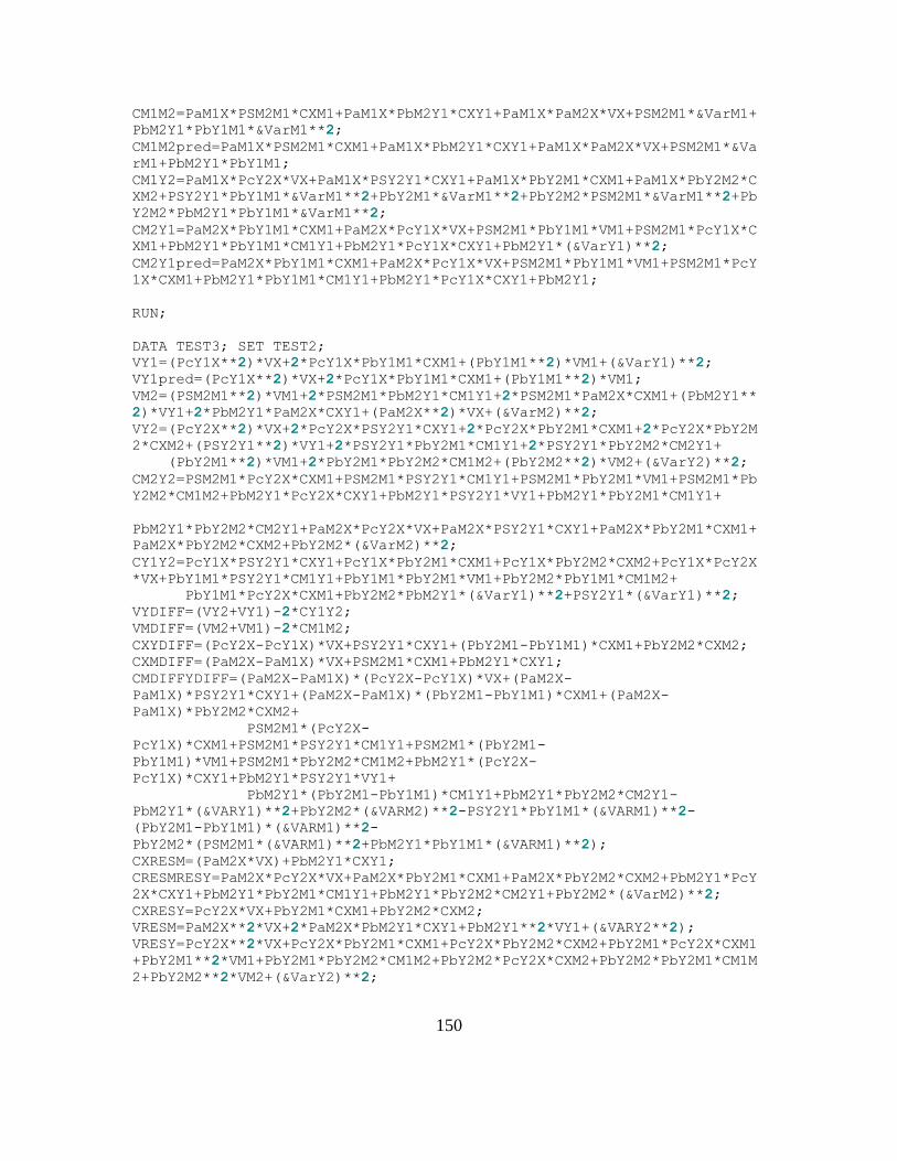
150
CM1M2=PaM1X*PSM2M1*CXM1+PaM1X*PbM2Y1*CXY1+PaM1X*PaM2X*VX+PSM2M1*&VarM1+
PbM2Y1*PbY1M1*&VarM1**2;
CM1M2pred=PaM1X*PSM2M1*CXM1+PaM1X*PbM2Y1*CXY1+PaM1X*PaM2X*VX+PSM2M1*&Va
rM1+PbM2Y1*PbY1M1;
CM1Y2=PaM1X*PcY2X*VX+PaM1X*PSY2Y1*CXY1+PaM1X*PbY2M1*CXM1+PaM1X*PbY2M2*C
XM2+PSY2Y1*PbY1M1*&VarM1**2+PbY2M1*&VarM1**2+PbY2M2*PSM2M1*&VarM1**2+Pb
Y2M2*PbM2Y1*PbY1M1*&VarM1**2;
CM2Y1=PaM2X*PbY1M1*CXM1+PaM2X*PcY1X*VX+PSM2M1*PbY1M1*VM1+PSM2M1*PcY1X*C
XM1+PbM2Y1*PbY1M1*CM1Y1+PbM2Y1*PcY1X*CXY1+PbM2Y1*(&VarY1)**2;
CM2Y1pred=PaM2X*PbY1M1*CXM1+PaM2X*PcY1X*VX+PSM2M1*PbY1M1*VM1+PSM2M1*PcY
1X*CXM1+PbM2Y1*PbY1M1*CM1Y1+PbM2Y1*PcY1X*CXY1+PbM2Y1;
RUN;
DATA TEST3; SET TEST2;
VY1=(PcY1X**2)*VX+2*PcY1X*PbY1M1*CXM1+(PbY1M1**2)*VM1+(&VarY1)**2;
VY1pred=(PcY1X**2)*VX+2*PcY1X*PbY1M1*CXM1+(PbY1M1**2)*VM1;
VM2=(PSM2M1**2)*VM1+2*PSM2M1*PbM2Y1*CM1Y1+2*PSM2M1*PaM2X*CXM1+(PbM2Y1**
2)*VY1+2*PbM2Y1*PaM2X*CXY1+(PaM2X**2)*VX+(&VarM2)**2;
VY2=(PcY2X**2)*VX+2*PcY2X*PSY2Y1*CXY1+2*PcY2X*PbY2M1*CXM1+2*PcY2X*PbY2M
2*CXM2+(PSY2Y1**2)*VY1+2*PSY2Y1*PbY2M1*CM1Y1+2*PSY2Y1*PbY2M2*CM2Y1+
(PbY2M1**2)*VM1+2*PbY2M1*PbY2M2*CM1M2+(PbY2M2**2)*VM2+(&VarY2)**2;
CM2Y2=PSM2M1*PcY2X*CXM1+PSM2M1*PSY2Y1*CM1Y1+PSM2M1*PbY2M1*VM1+PSM2M1*Pb
Y2M2*CM1M2+PbM2Y1*PcY2X*CXY1+PbM2Y1*PSY2Y1*VY1+PbM2Y1*PbY2M1*CM1Y1+
PbM2Y1*PbY2M2*CM2Y1+PaM2X*PcY2X*VX+PaM2X*PSY2Y1*CXY1+PaM2X*PbY2M1*CXM1+
PaM2X*PbY2M2*CXM2+PbY2M2*(&VarM2)**2;
CY1Y2=PcY1X*PSY2Y1*CXY1+PcY1X*PbY2M1*CXM1+PcY1X*PbY2M2*CXM2+PcY1X*PcY2X
*VX+PbY1M1*PSY2Y1*CM1Y1+PbY1M1*PbY2M1*VM1+PbY2M2*PbY1M1*CM1M2+
PbY1M1*PcY2X*CXM1+PbY2M2*PbM2Y1*(&VarY1)**2+PSY2Y1*(&VarY1)**2;
VYDIFF=(VY2+VY1)-2*CY1Y2;
VMDIFF=(VM2+VM1)-2*CM1M2;
CXYDIFF=(PcY2X-PcY1X)*VX+PSY2Y1*CXY1+(PbY2M1-PbY1M1)*CXM1+PbY2M2*CXM2;
CXMDIFF=(PaM2X-PaM1X)*VX+PSM2M1*CXM1+PbM2Y1*CXY1;
CMDIFFYDIFF=(PaM2X-PaM1X)*(PcY2X-PcY1X)*VX+(PaM2X-
PaM1X)*PSY2Y1*CXY1+(PaM2X-PaM1X)*(PbY2M1-PbY1M1)*CXM1+(PaM2X-
PaM1X)*PbY2M2*CXM2+
PSM2M1*(PcY2X-
PcY1X)*CXM1+PSM2M1*PSY2Y1*CM1Y1+PSM2M1*(PbY2M1-
PbY1M1)*VM1+PSM2M1*PbY2M2*CM1M2+PbM2Y1*(PcY2X-
PcY1X)*CXY1+PbM2Y1*PSY2Y1*VY1+
PbM2Y1*(PbY2M1-PbY1M1)*CM1Y1+PbM2Y1*PbY2M2*CM2Y1-
PbM2Y1*(&VARY1)**2+PbY2M2*(&VARM2)**2-PSY2Y1*PbY1M1*(&VARM1)**2-
(PbY2M1-PbY1M1)*(&VARM1)**2-
PbY2M2*(PSM2M1*(&VARM1)**2+PbM2Y1*PbY1M1*(&VARM1)**2);
CXRESM=(PaM2X*VX)+PbM2Y1*CXY1;
CRESMRESY=PaM2X*PcY2X*VX+PaM2X*PbY2M1*CXM1+PaM2X*PbY2M2*CXM2+PbM2Y1*PcY
2X*CXY1+PbM2Y1*PbY2M1*CM1Y1+PbM2Y1*PbY2M2*CM2Y1+PbY2M2*(&VarM2)**2;
CXRESY=PcY2X*VX+PbY2M1*CXM1+PbY2M2*CXM2;
VRESM=PaM2X**2*VX+2*PaM2X*PbM2Y1*CXY1+PbM2Y1**2*VY1+(&VARY2**2);
VRESY=PcY2X**2*VX+PcY2X*PbY2M1*CXM1+PcY2X*PbY2M2*CXM2+PbY2M1*PcY2X*CXM1
+PbY2M1**2*VM1+PbY2M1*PbY2M2*CM1M2+PbY2M2*PcY2X*CXM2+PbY2M2*PbY2M1*CM1M
2+PbY2M2**2*VM2+(&VarY2)**2;

151
/*USED TO CALCULATE MSE FOR M2 EQUATION AND Y2 EQUATION CORRESPONDING
TO TWO-WAVE MODEL*/
VM2PRED=(PaM2X**2)*VX+2*PaM2X*PSM2M1*CXM1+(PSM2M1**2)*VM1;
VY2PRED=(PcY2X**2)*VX+2*PcY2X*PSY2Y1*CXY1+2*PcY2X*PbY2M1*CXM1+2*PcY2X*P
bY2M2*CXM2+(PSY2Y1**2)*VY1pred+2*PSY2Y1*PbY2M1*CM1Y1pred+2*PSY2Y1*PbY2M
2*CM2Y1pred+
(PbY2M1**2)*VM1+2*PbY2M1*PbY2M2*CM1M2pred+(PbY2M2**2)*VM2pred;
RUN;
DATA TEST4; SET TEST3;
STDX=SQRT(VX);
STDM1=SQRT(VM1);
STDY1=SQRT(VY1);
STDM2=SQRT(VM2);
STDY2=SQRT(VY2);
STDMDIFF=SQRT(VMDIFF);
STDYDIFF=SQRT(VYDIFF);
STDMres=SQRT(VRESM);
STDYres=SQRT(VRESY);
RUN;
/*Zero-order correlations*/
DATA TEST5; SET TEST4;
RXM1=CXM1/(STDX*STDM1);
RXY1=CXY1/(STDX*STDY1);
RXM2=CXM2/(STDX*STDM2);
RXY2=CXY2/(STDX*STDY2);
RM1Y1=CM1Y1/(STDM1*STDY1);
RM1M2=CM1M2/(STDM1*STDM2);
RM1Y2=CM1Y2/(STDM1*STDY2);
RM2Y1=CM2Y1/(STDM2*STDY1);
RM2Y2=CM2Y2/(STDM2*STDY2);
RY1Y2=CY1Y2/(STDY1*STDY2);
RXMDIFF=cxmdiff/(STDX*STDMDIFF);
RXYDIFF=cxydiff/(STDX*STDYDIFF);
RMYDIFF=cmdiffydiff/(STDMDIFF*STDYDIFF);
RXMres=cxresm/(STDX*STDMres);
RXYres=cxresy/(STDX*STDYres);
RMYres=cresmresy/(STDMres*STDYres);
RUN;
/*First-Order partial correlations. Variable partialed out is at the
beginning of the variable name*/
DATA TEST6; SET TEST5;
m1RXY1=(RXY1-(RM1Y1*RXM1))/(SQRT(1-RM1Y1**2)*SQRT(1-RXM1**2));
xRM1Y1=(RM1Y1-(RXM1*RXY1))/(SQRT(1-RXM1**2)*SQRT(1-RXY1**2));
m1RXM2=(RXM2-(RXM1*RM1M2))/(SQRT(1-RXM1**2)*SQRT(1-RM1M2**2));
y1RXM2=(RXM2-(RXY1*RM2Y1))/(SQRT(1-RXY1**2)*SQRT(1-RM2Y1**2));
y1RXY2=(RXY2-(RXY1*RY1Y2))/(SQRT(1-RXY1**2)*SQRT(1-RY1Y2**2));
m2RXY2=(RXY2-(RXM2*RM2Y2))/(SQRT(1-RXM2**2)*SQRT(1-RM2Y2**2));
m1RY1M2=(RM2Y1-(RM1Y1*RM1M2))/(SQRT(1-RM1Y1**2)*SQRT(1-RM1M2**2));
xRY1M2=(RM2Y1-(RXY1*RXM2))/(SQRT(1-RXY1**2)*SQRT(1-RXM2**2));

152
xRM1M2=(RM1M2-(RXM1*RXM2))/(SQRT(1-RXM1**2)*SQRT(1-RXM2**2));
y1RM1M2=(RM1M2-(RM1Y1*RM2Y1))/(SQRT(1-RM1Y1**2)*SQRT(1-RM2Y1**2));
xRM1Y2=(RM1Y2-(RXM1*RXY2))/(SQRT(1-RXM1**2)*SQRT(1-RXY2**2));
y1RM1Y2=(RM1Y2-(RM1Y1*RY1Y2))/(SQRT(1-RM1Y1**2)*SQRT(1-RY1Y2**2));
m2RM1Y2=(RM1Y2-(RM1M2*RM2Y2))/(SQRT(1-RM1M2**2)*SQRT(1-RM2Y2**2));
xRM2Y2=(RM2Y2-(RXM2*RXY2))/(SQRT(1-RXM2**2)*SQRT(1-RXY2**2));
y1RM2Y2=(RM2Y2-(RM2Y1*RY1Y2))/(SQRT(1-RM2Y1**2)*SQRT(1-RY1Y2**2));
m1RM2Y2=(RM2Y2-(RM1M2*RM1Y2))/(SQRT(1-RM1M2**2)*SQRT(1-RM1Y2**2));
xRY1Y2=(RY1Y2-(RXY1*RXY2))/(SQRT(1-RXY1**2)*SQRT(1-RXY2**2));
m1RY1Y2=(RY1Y2-(RM1Y1*RM1Y2))/(SQRT(1-RM1Y1**2)*SQRT(1-RM1Y2**2));
m2RY1Y2=(RY1Y2-(RM2Y1*RM2Y2))/(SQRT(1-RM2Y1**2)*SQRT(1-RM2Y2**2));
m1RXY2=(RXY2-(RXM1*RM1Y2))/(SQRT(1-RXM1**2)*SQRT(1-RM1Y2**2));
y1RXM1=(RXM2-(RXY1*RM1Y1))/(SQRT(1-RXY1**2)*SQRT(1-RM1Y1**2));
xRMYDiff=(RMYdiff-(RXMdiff*RXYdiff))/(SQRT(1-RXMdiff**2)*SQRT(1-
RXYdiff**2));
/*Second-order partial correlations. Variables partialed out are at the
beginning of the variable name*/
m1y1RXM2=(m1RXM2-(m1RY1M2*m1RXY1))/(SQRT(1-m1RY1M2**2)*SQRT(1-
m1RXY1**2));
m1y1RXY2=(m1RXY2-(m1RXY1*m1RY1Y2))/(SQRT(1-m1RXY1**2)*SQRT(1-
m1RY1Y2**2));
y1m2RXY2=(y1RXY2-(y1RXM2*y1RM2Y2))/(SQRT(1-y1RXM2**2)*SQRT(1-
y1RM2Y2**2));
m1m2RXY2=(m1RXY2-(m1RXM2*m1RM2Y2))/(SQRT(1-m1RXM2**2)*SQRT(1-
m1RM2Y2**2));
xy1RM1M2=(xRM1M2-(xRM1Y1*xRY1M2))/(SQRT(1-xRM1Y1**2)*SQRT(1-
xRY1M2**2));
xy1RM1Y2=(xRM1Y2-(xRM1Y1*xRY1Y2))/(SQRT(1-xRM1Y1**2)*SQRT(1-
xRY1Y2**2));
y1m2RM1Y2=(y1RM1Y2-(y1RM1M2*y1RM2Y2))/(SQRT(1-y1RM1M2**2)*SQRT(1-
y1RM2Y2**2));
xm2RM1Y2=(xRM1Y2-(xRM1M2*xRM2Y2))/(SQRT(1-xRM1M2**2)*SQRT(1-
xRM2Y2**2));
xm1RY1M2=(xRY1M2-(xRM1Y1*xRM1M2))/(SQRT(1-xRM1Y1**2)*SQRT(1-
xRM1M2**2));
xy1RM2Y2=(xRM2Y2-(xRY1M2*xRY1Y2))/(SQRT(1-xRY1M2**2)*SQRT(1-
xRY1Y2**2));
xm1RM2Y2=(xRM2Y2-(xRM1M2*xRM1Y2))/(SQRT(1-xRM1M2**2)*SQRT(1-
xRM1Y2**2));
y1m1RM2Y2=(y1RM2Y2-(y1RM1M2*y1RM1Y2))/(SQRT(1-y1RM1M2**2)*SQRT(1-
y1RM1Y2**2));
xm1RY1Y2=(xRY1Y2-(xRM1Y1*xRM1Y2))/(SQRT(1-xRM1Y1**2)*SQRT(1-
xRM1Y2**2));
xm2RY1Y2=(xRY1Y2-(xRY1M2*xRM2Y2))/(SQRT(1-xRY1M2**2)*SQRT(1-
xRM2Y2**2));
m1m2RY1Y2=(m1RY1Y2-(m1RY1M2*m1RM2Y2))/(SQRT(1-m1RY1M2**2)*SQRT(1-
m1RM2Y2**2));
y1m2RXM1=(y1RXM1-(y1RXM2*y1RM1M2))/(SQRT(1-y1RXM2**2)*SQRT(1-
y1RM1M2**2));
m1m2RXY1=(m1RXY1-(m1RXM2*m1RY1M2))/(SQRT(1-m1RXY1**2)*SQRT(1-
m1RY1M2**2));

153
xm2RM1Y1=(xRM1Y1-(xRM1M2*xRY1M2))/(SQRT(1-xRM1Y1**2)*SQRT(1-
xRY1M2**2));
/*Third-order partial correlations. Variables partialed out are at the
beginning of the variable name*/
y1m1m2RXY2=(m1y1RXY2-(m1y1RXM2*y1m1RM2Y2))/(SQRT(1-m1y1RXM2**2)*SQRT(1-
y1m1RM2Y2**2));
y1xm2RM1Y2=(xy1RM1Y2-(xy1RM1M2*xy1RM2Y2))/(SQRT(1-xy1RM1M2**2)*SQRT(1-
xy1RM2Y2**2));
xm1m2RY1Y2=(xm1RY1Y2-(xm1RY1M2*xm1RM2Y2))/(SQRT(1-xm1RY1M2**2)*SQRT(1-
xm1RM2Y2**2));
xm1y1RM2Y2=(xm1RM2Y2-(xm1RY1M2*xm1RY1Y2))/(SQRT(1-xm1RY1M2**2)*SQRT(1-
xm1RY1Y2**2));
/*True value of bY2M2 coefficient and product of AB under the
difference score model and residualized change score model*/
TrueBYMDiff=((RMYdiff-(RXMdiff*RXYdiff))/(1-
RXMdiff**2))*(stdydiff/stdmdiff);
TrueBYMRES=((RMYRES-(RXMRES*RXYRES))/(1-RXMRES**2))*(stdyres/stdmres);
TrueABDIFF=Pam2X*TrueBYMDiff;
TrueABRes=Pam2X*TrueBYMRES;
/*Bias of AB under the difference score and residualized change score
model*/
BBDiffalt=bY2M2diff-trueBymdiff;
BBDiffaltR=BBDiffalt/trueBymdiff;
B2BDiffalt=BBDiffalt**2;
LbY2M2diffalt=bY2M2Diff-1.96*SEbY2M2Diff;
UbY2M2Diffalt=bY2M2Diff+1.96*SEbY2M2Diff;
RGbY2M2Diffalt=0; LFbY2M2Diffalt=0;
If trueBYMDiff GT UbY2M2Diffalt then RGbY2M2Diffalt=1;
If trueBYMDiff LT LbY2M2Diffalt then LFbY2M2Diffalt=1;
CVGbY2M2Diffalt=1-(RGbY2M2Diffalt+LFbY2M2Diffalt);
BABDIFF=ABDIFF-TRUEABDiff;
BABDIFFR=BABDIFF/TRUEABDiff;
B2ABDIFF=BABDIFF**2;
BABRES=ABRES-TRUEABRES;
BABRESR=BABRES/TRUEABRES;
B2ABRES=BABRES**2;
RUN;
/*Estimated partial correlations to test the analytic formulas*/
/*First-order partial correlations*/
PROC CORR DATA=SIM OUTPUT=CORRTEST NOPRINT; by rep;
VAR X Y1;
PARTIAL M1;
DATA PC1; SET CORRTEST; IF _NAME_= 'Y1'; m1CORRXY1=X;
KEEP m1CORRXY1;
PROC CORR DATA=SIM OUTPUT=CORRTEST NOPRINT; by rep;
VAR M1 Y1;
PARTIAL X;
DATA PC2; SET CORRTEST; IF _NAME_= 'Y1'; xCORRM1Y1=M1;

154
KEEP xCORRM1Y1;
PROC CORR DATA=SIM OUTPUT=CORRTEST NOPRINT; by rep;
VAR X M2;
PARTIAL M1;
DATA PC3; SET CORRTEST; IF _NAME_= 'M2'; m1CORRXM2=X;
KEEP m1CORRXM2;
PROC CORR DATA=SIM OUTPUT=CORRTEST NOPRINT; by rep;
VAR X M2;
PARTIAL y1;
DATA PC4; SET CORRTEST; IF _NAME_= 'M2'; y1CORRXM2=X;
KEEP y1CORRXM2;
PROC CORR DATA=SIM OUTPUT=CORRTEST NOPRINT; by rep;
VAR X Y2;
PARTIAL y1;
DATA PC5; SET CORRTEST; IF _NAME_= 'Y2'; y1CORRXY2=X;
KEEP y1CORRXY2;
PROC CORR DATA=SIM OUTPUT=CORRTEST NOPRINT; by rep;
VAR X Y2;
PARTIAL M2;
DATA PC6; SET CORRTEST; IF _NAME_= 'Y2'; m2CORRXY2=X;
KEEP m2CORRXY2;
PROC CORR DATA=SIM OUTPUT=CORRTEST NOPRINT; by rep;
VAR y1 M2;
PARTIAL M1;
DATA PC7; SET CORRTEST; IF _NAME_= 'M2'; m1CORRY1M2=y1;
KEEP m1CORRY1M2;
PROC CORR DATA=SIM OUTPUT=CORRTEST NOPRINT; by rep;
VAR y1 M2;
PARTIAL X;
DATA PC8; SET CORRTEST; IF _NAME_= 'M2'; xCORRY1M2=y1;
KEEP xCORRY1M2;
PROC CORR DATA=SIM OUTPUT=CORRTEST NOPRINT; by rep;
VAR M1 M2;
PARTIAL X;
DATA PC9; SET CORRTEST; IF _NAME_= 'M2'; xCORRM1M2=M1;
KEEP xCORRM1M2;
PROC CORR DATA=SIM OUTPUT=CORRTEST NOPRINT; by rep;
VAR M1 M2;
PARTIAL y1;
DATA PC10; SET CORRTEST; IF _NAME_= 'M2'; y1CORRM1M2=M1;
KEEP y1CORRM1M2;
PROC CORR DATA=SIM OUTPUT=CORRTEST NOPRINT; by rep;
VAR M1 Y2;
PARTIAL X;
DATA PC11; SET CORRTEST; IF _NAME_= 'Y2'; xCORRM1Y2=M1;

155
KEEP xCORRM1Y2;
PROC CORR DATA=SIM OUTPUT=CORRTEST NOPRINT; by rep;
VAR M1 Y2;
PARTIAL y1;
DATA PC12; SET CORRTEST; IF _NAME_= 'Y2'; y1CORRM1Y2=M1;
KEEP y1CORRM1Y2;
PROC CORR DATA=SIM OUTPUT=CORRTEST NOPRINT; by rep;
VAR M1 Y2;
PARTIAL M2;
DATA PC13; SET CORRTEST; IF _NAME_= 'Y2'; m2CORRM1Y2=M1;
KEEP m2CORRM1Y2;
PROC CORR DATA=SIM OUTPUT=CORRTEST NOPRINT; by rep;
VAR M2 Y2;
PARTIAL X;
DATA PC14; SET CORRTEST; IF _NAME_= 'Y2'; xCORRM2Y2=M2;
KEEP xCORRM2Y2;
PROC CORR DATA=SIM OUTPUT=CORRTEST NOPRINT; by rep;
VAR M2 Y2;
PARTIAL y1;
DATA PC15; SET CORRTEST; IF _NAME_= 'Y2'; y1CORRM2Y2=M2;
KEEP y1CORRM2Y2;
PROC CORR DATA=SIM OUTPUT=CORRTEST NOPRINT; by rep;
VAR M2 Y2;
PARTIAL M1;
DATA PC16; SET CORRTEST; IF _NAME_= 'Y2'; m1CORRM2Y2=M2;
KEEP m1CORRM2Y2;
PROC CORR DATA=SIM OUTPUT=CORRTEST NOPRINT; by rep;
VAR y1 Y2;
PARTIAL X;
DATA PC17; SET CORRTEST; IF _NAME_= 'Y2'; xCORRY1Y2=y1;
KEEP xCORRY1Y2;
PROC CORR DATA=SIM OUTPUT=CORRTEST NOPRINT; by rep;
VAR y1 Y2;
PARTIAL M1;
DATA PC18; SET CORRTEST; IF _NAME_= 'Y2'; m1CORRY1Y2=y1;
KEEP m1CORRY1Y2;
PROC CORR DATA=SIM OUTPUT=CORRTEST NOPRINT; by rep;
VAR y1 Y2;
PARTIAL M2;
DATA PC19; SET CORRTEST; IF _NAME_= 'Y2'; m2CORRY1Y2=y1;
KEEP m2CORRY1Y2;
PROC CORR DATA=SIM OUTPUT=CORRTEST NOPRINT; by rep;
VAR X Y2;
PARTIAL M1;
DATA PC20; SET CORRTEST; IF _NAME_= 'Y2'; m1CORRXY2=X;
156
KEEP m1CORRXY2;
PROC CORR DATA=SIM OUTPUT=CORRTEST NOPRINT; by rep;
VAR X M1;
PARTIAL M2;
DATA PC21; SET CORRTEST; IF _NAME_= 'M1'; m2CORRXM1=X;
KEEP m2CORRXM1;
PROC CORR DATA=SIM OUTPUT=CORRTEST NOPRINT; by rep;
VAR X Y1;
PARTIAL M2;
DATA PC22; SET CORRTEST; IF _NAME_= 'Y1'; m2CORRXY1=X;
KEEP m2CORRXY1;
/*Second-Order partial correlations*/
PROC CORR DATA=SIM OUTPUT=CORRTEST NOPRINT; by rep;
VAR X M2;
PARTIAL M1 y1;
DATA PC23; SET CORRTEST; IF _NAME_= 'M2'; m1y1CORRXM2=X;
KEEP m1y1CORRXM2;
PROC CORR DATA=SIM OUTPUT=CORRTEST NOPRINT; by rep;
VAR X Y2;
PARTIAL M1 y1;
DATA PC24; SET CORRTEST; IF _NAME_= 'Y2'; m1y1CORRXY2=X;
KEEP m1y1CORRXY2;
PROC CORR DATA=SIM OUTPUT=CORRTEST NOPRINT; by rep;
VAR X Y2;
PARTIAL y1 M2;
DATA PC25; SET CORRTEST; IF _NAME_= 'Y2'; y1m2CORRXY2=X;
KEEP y1m2CORRXY2;
PROC CORR DATA=SIM OUTPUT=CORRTEST NOPRINT; by rep;
VAR X Y2;
PARTIAL M1 M2;
DATA PC26; SET CORRTEST; IF _NAME_= 'Y2'; m1m2CORRXY2=X;
KEEP m1m2CORRXY2;
PROC CORR DATA=SIM OUTPUT=CORRTEST NOPRINT; by rep;
VAR M1 M2;
PARTIAL X y1;
DATA PC27; SET CORRTEST; IF _NAME_= 'M2'; xy1CORRM1M2=M1;
KEEP xy1CORRM1M2;
PROC CORR DATA=SIM OUTPUT=CORRTEST NOPRINT; by rep;
VAR M1 Y2;
PARTIAL X y1;
DATA PC28; SET CORRTEST; IF _NAME_= 'Y2'; xy1CORRM1Y2=M1;
KEEP xy1CORRM1Y2;
PROC CORR DATA=SIM OUTPUT=CORRTEST NOPRINT; by rep;
VAR M1 Y2;

157
PARTIAL y1 M2;
DATA PC29; SET CORRTEST; IF _NAME_= 'Y2'; y1m2CORRM1Y2=M1;
KEEP y1m2CORRM1Y2;
PROC CORR DATA=SIM OUTPUT=CORRTEST NOPRINT; by rep;
VAR M1 Y2;
PARTIAL X M2;
DATA PC30; SET CORRTEST; IF _NAME_= 'Y2'; xm2CORRM1Y2=M1;
KEEP xm2CORRM1Y2;
PROC CORR DATA=SIM OUTPUT=CORRTEST NOPRINT; by rep;
VAR y1 M2;
PARTIAL X M1;
DATA PC31; SET CORRTEST; IF _NAME_= 'M2'; xm1CORRY1M2=y1;
KEEP xm1CORRY1M2;
PROC CORR DATA=SIM OUTPUT=CORRTEST NOPRINT; by rep;
VAR M2 Y2;
PARTIAL X y1;
DATA PC32; SET CORRTEST; IF _NAME_= 'Y2'; xy1CORRM2Y2=M2;
KEEP xy1CORRM2Y2;
PROC CORR DATA=SIM OUTPUT=CORRTEST NOPRINT; by rep;
VAR M2 Y2;
PARTIAL X M1;
DATA PC33; SET CORRTEST; IF _NAME_= 'Y2'; xm1CORRM2Y2=M2;
KEEP xm1CORRM2Y2;
PROC CORR DATA=SIM OUTPUT=CORRTEST NOPRINT; by rep;
VAR M2 Y2;
PARTIAL Y1 M1;
DATA PC34; SET CORRTEST; IF _NAME_= 'Y2'; y1m1CORRM2Y2=M2;
KEEP y1m1CORRM2Y2;
PROC CORR DATA=SIM OUTPUT=CORRTEST NOPRINT; by rep;
VAR y1 Y2;
PARTIAL X M1;
DATA PC35; SET CORRTEST; IF _NAME_= 'Y2'; xm1CORRY1Y2=y1;
KEEP xm1CORRY1Y2;
PROC CORR DATA=SIM OUTPUT=CORRTEST NOPRINT; by rep;
VAR y1 Y2;
PARTIAL X M2;
DATA PC36; SET CORRTEST; IF _NAME_= 'Y2'; xm2CORRY1Y2=y1;
KEEP xm2CORRY1Y2;
PROC CORR DATA=SIM OUTPUT=CORRTEST NOPRINT; by rep;
VAR y1 Y2;
PARTIAL M1 M2;
DATA PC37; SET CORRTEST; IF _NAME_= 'Y2';m1m2CORRY1Y2=y1;
KEEP m1m2CORRY1Y2;
/*Third-Order partial correlations*/
PROC CORR DATA=SIM OUTPUT=CORRTEST NOPRINT; by rep;

158
VAR X Y2;
PARTIAL y1 M1 M2;
DATA PC38; SET CORRTEST; IF _NAME_= 'Y2';y1m1m2CORRXY2=X;
KEEP y1m1m2CORRXY2;
PROC CORR DATA=SIM OUTPUT=CORRTEST NOPRINT; by rep;
VAR M1 Y2;
PARTIAL y1 X M2;
DATA PC39; SET CORRTEST; IF _NAME_= 'Y2';y1xm2CORRM1Y2=M1;
KEEP y1xm2CORRM1Y2;
PROC CORR DATA=SIM OUTPUT=CORRTEST NOPRINT; by rep;
VAR Y1 Y2;
PARTIAL X M1 M2;
DATA PC40; SET CORRTEST; IF _NAME_= 'Y2';xm1m2CORRY1Y2=Y1;
KEEP xm1m2CORRY1Y2;
PROC CORR DATA=SIM OUTPUT=CORRTEST NOPRINT; by rep;
VAR M2 Y2;
PARTIAL X M1 y1;
DATA PC41; SET CORRTEST; IF _NAME_= 'Y2';xm1y1CORRM2Y2=M2;
KEEP xm1y1CORRM2Y2;
RUN;
DATA PARTCORR; MERGE PC1 PC2 PC3 PC4 PC5 PC6 PC7 PC8 PC9 PC10 PC11 PC12
PC13 PC14 PC15 PC16 PC17 PC18 PC19 PC20 PC21 PC22 PC23 PC24
PC25 PC26 PC27 PC28 PC29 PC30 PC31 PC32 PC33 PC34 PC35 PC36 PC37 PC38
PC39 PC40 PC41;
RUN;
DATA ALLCORR; MERGE SCOVS SCORRS PARTCORR;
/*True Standard errors*/
DATA TEST7; SET TEST6;
TRUEMSEM2=VM2-VM2PRED;
TRUESEA=sqrt((TRUEMSEM2/(NOBS-1))*((1/VX)/(1-m1RXM2**2)));
TRUEMSEY2=VY2-VY2PRED;
TRUESEB=SQRT((TRUEMSEY2)/((NOBS-1))*((1/VM2)/(1-xm1y1RM2Y2**2)));
TRUESEC=SQRT((TRUEMSEY2)/((NOBS-1))*((1/VX)/(1-y1m1m2RXY2**2)));
TRUESEAB=SQRT((PaM2X**2)*(TRUESEB**2)+(PbY2M2**2)*(TRUESEA**2));
*The following computes the Bias, Bias squared, and relative Bias for
the standard errors;
BSEA=SEaM2X-TrueSEA;
BSEAR=BSEA/TrueSEA;
B2SEA=BSEA**2;
BSEB=SEbY2M2-TrueSEB;
BSEBR=BSEB/TrueSEB;
B2SEB=BSEB**2;
BSEC=SEcY2X-TrueSEC;
BSECR=BSEC/TrueSEC;
B2SEC=BSEC**2;
BSEADIFF=SEaM2Xdiff-TrueSEA;
BSEADIFFR=BSEADIFF/TrueSEA;
B2SEADIFF=BSEADIFF**2;
159
BSEBDIFF=SEbY2M2Diff-TrueSEB;
BSEBDIFFR=BSEBDIFF/TrueSEB;
B2SEBDIFF=BSEBDIFF**2;
BSECDIFF=SEcY2XDIFF-TrueSEC;
BSECDIFFR=BSECDIFF/TrueSEC;
B2SECDIFF=BSECDIFF**2;
BSEARES=SEaM2XRES-TrueSEA;
BSEARESR=BSEARES/TrueSEA;
B2SEARES=BSEARES**2;
BSEBRES=SEbY2M2RES-TrueSEB;
BSEBRESR=BSEBRES/TrueSEB;
B2SEBRES=BSEBRES**2;
BSECRES=SEcY2XRES-TrueSEC;
BSECRESR=BSECRES/TrueSEC;
B2SECRES=BSECRES**2;
BSEA_=SEaM2X_-TrueSEA;
BSEA_R=BSEA_/TrueSEA;
B2SEA_=BSEA_**2;
BSEB_=SEbY2M2_-TrueSEB;
BSEB_R=BSEB_/TrueSEB;
B2SEB_=BSEB_**2;
BSEC_=SEcY2X_-TrueSEC;
BSEC_R=BSEC_/TrueSEC;
B2SEC_=BSEC_**2;
BSEAB=SEAB-TRUESEAB;
BSEABR=BSEAB/TRUESEAB;
B2SEAB=BSEAB**2;
BSEABDIFF=SEABDIFF-TRUESEAB;
BSEABDIFFR=BSEABDIFF/TRUESEAB;
B2SEABDIFF=BSEABDIFF**2;
BSEABRES=SEABRES-TRUESEAB;
BSEABRESR=BSEABRES/TRUESEAB;
B2SEABRES=BSEABRES**2;
BSEAB_=SEAB_-TRUESEAB;
BSEAB_R=BSEAB_/TRUESEAB;
B2SEAB_=BSEAB_**2;
RUN;
DATA ALLDAT; MERGE TEST7 ALLCORR;
run;
DATA DATAOUT.&FILE.outalt; SET ALLDAT;
RUN;
%MEND;
run;
PROC DATASETS LIB=WORK NOLIST;
%ANALYZE(nsim=1000,nobs=50,BMX=0,BYX=0,BYM=0,
aM1X=0, sm2m1=.981,am2x=0,bm2y1=0, by1m1=.578,
cy1x=0, cy2x=0,sy2y1=.686, by2m1=0,by2m2=0,
varx=1,varm1=1,varm2=1,vary1=1,vary2=1,
RELM1=1, RELM2=1, RELY1=1, RELY2=1,
FILE=n50cond1,TYPE='CCC',ERROR=1); run; quit;

160
APPENDIX G
SAS MACRO CALLING PRODCLIN TO ESTIMATE CONFIDENCE INTERVALS
FOR THE MEDIATED EFFECT FOR THE ANCOVA MODEL

161
*Using PRODCLIN to estimate asymmetric confidence intervals for the
mediated effect for ANCOVA;
FILENAME NULLOG DUMMY 'C:\NULL';
PROC PRINTTO LOG=NULLOG;
libname DATAOUT "D:\Valente Masters Sim\DATAOUT\";
libname PRODOUT "D:\Valente Masters Sim\PRODOUT\";
*proc printto log=dum;
*options nosource nonotes;
%MACRO CONFLIM(FILE);
PROC DATASETS LIBRARY=WORK KILL NOLIST; RUN;
DATA PRODCLIN; set DATAOUT.&file;
run;
data test; length ii $8; set PRODCLIN;
i+1;
ii=left(put(i, 8.));
call symput ('b'||ii, by2m2);
call symput ('a'||ii, am2x);
call symput ('seb'||ii,seby2m2);
call symput ('sea'||ii,seam2x);
call symput ('nobs', _n_);
run;
options noxwait ;
*Designate location of prdclinforSAS.sas and prodclinsas2.exe;
Data summary;
%macro prodclin(a, sea, b, seb, rho, alpha);
data data1;
*Change file address to match the location of the file prodclin.exe;
file "D:\Valente Masters Sim\raw.txt";
a=&a; sea=&sea; b=&b; seb=&seb; rho=ρ alpha=α
put a @; put sea @; put b @; put seb @; put rho @; put alpha @;
run;
*Change file address to match the location of the file prodclin.exe;
X cd D:\Valente Masters Sim\;
*Change file address to match the location of the file prodclin.exe;
X call "D:\Valente Masters Sim\ProdClin2_Sas.exe";
data data2;
do;

162
rc=system("D:\Valente Masters Sim\ProdClin2_Sas.exe");
end;
run;
data data2;
infile "D:\Valente Masters Sim\critval.txt";
input lowz highz;
a=&a; sea=&sea; b=&b; seb=&seb; rho=ρ alpha=α
r=rho;
da=a/sea;
db=b/seb;
sedadb=sqrt(da*da+db*db+1);
dadb=da*db;
ab=a*b;
sobelse=sqrt(a*a*seb*seb+b*b*sea*sea);
se_ab=sobelse;
MVDSE = sqrt(a*a*seb*seb+b*b*sea*sea);
prodlow=lowz;
produp=highz;
nl=probit(alpha/2);
normlow=ab+nl*se_ab;
normup=ab-nl*se_ab;
TesT_SE = sqrt(A*a*seb*seb+b*b*sea*sea+2*a*b*r*sea*seb-
(r*sea*seb)*(r*sea*seb)+sea*sea*seb*seb);
run;
*proc print data=data2 noobs;
*var a sea b seb ab rho alpha prodlow produp Test_SE;
*run;
data summary; set summary data2;
keep a b seb sea ab prodlow produp normlow normup;
run;
%mend prodclin;
%macro prodclinbootstrap;
%do i=1 %to &nobs;
%prodclin (a=&&a&i, sea=&&sea&i, b=&&b&i, seb=&&seb&i, rho=0, alpha =
.05);
%end;
%mend prodclinbootstrap;
%prodclinbootstrap;
run;
data prodout.&file.prodANCOVA; set summary;
if _n_=1 then delete;
run;
%mend CONFLIM;
%conflim(FILE=n50cond1out);

163
APPENDIX H
SAS MACRO CREATING PERCENTILE BOOTSTRAPPED CONFIDENCE
INTERVALS FOR ALL MODELS

164
*Creating Percentile Bootstrapped CIs for the mediated effect for all
models;
libname DATAGEN "C:\Users\psyripl\Desktop\";
libname DATABOOT "D:\Valente Masters Sim\DATABOOT\";
FILENAME NULLOG DUMMY 'C:\NULL';
PROC PRINTTO LOG=NULLOG; run;
%Macro Bootstrap (nsim,nobs,BMX,BYX,BYM,
aM1X, sm2m1,am2x,bm2y1,by1m1,
cy1x,cy2x,sy2y1, by2m1,by2m2,
varx,varm1,varm2,vary1,vary2,
RELM1, RELM2, RELY1, RELY2,
FILE,TYPE,ERROR);
DATA SIM; SET DATAGEN.&file;
J=&nobs;
DO J=0 to totaln by &nobs;
IF 1+J<=I<=&nobs+J then Key=1+(J/&nobs);
end;
keep I X M1 M2 Y1 Y2 MDIFF YDIFF Key file;
run;
*Resampling;
%let nboot=1000;
proc surveyselect data=SIM noprint out=outtemp method=urs
sampsize=&nobs rep=&nboot outhits;
by Key;
run;
quit;
/***************************************************************/
/* */
/* PATH MODEL */
/* */
/***************************************************************/
PROC CALIS DATA=outtemp METHOD=ML NORPINT PLC OUTEST=OUT1 outstat=out2;
by key replicate;
LINEQS
M2=sm2m1_ M1 + am2x_ X + E2,
y2=cy2x_ X + sy2y1_ y1 + by2m1_ M1 + by2m2_ M2 + E3;
Cov
X M1,
X Y1,
M1 Y1;
STD
E2 = EE2,
E3 = EE3;
RUN;
*SAVING THE PARAMETER VALUES OF FROM THE PATH MODEL OUTPUT. PARAMETERS
ARE DENOTED WITH _ AT THE END OF THE NAME;
DATA CALPARMS; SET OUT1;
IF _TYPE_="PARMS";

165
KEEP aM2X_ bY2M2_ key replicate;
run;
/***************************************************************/
/* */
/* CHANGE SCORES */
/* */
/***************************************************************/
/*ESTIMATING (DIFFM=X Y1) REGRESSION AND SAVING THE VALUES OF THE
COEFFICIENTS AND THEIR STANDARD ERRORS*/
PROC REG DATA=outtemp OUTEST=DiffFILE1 COVOUT noprint; by key
replicate; MODEL Mdiff= X/;
DATA DiffA; SET DiffFILE1; IF _TYPE_='PARMS'; aM2XDiff=X;
DROP _MODEL_ _NAME_ _TYPE_ _DEPVAR_ _RMSE_ INTERCEP X;
KEEP aM2XDiff key replicate;
run;
*Estimating the (DiffY=X DiffM) REGRESSION AND SAVING THE VALUES OF THE
COEFFICIENTS AND THEIR STANDARD ERRORS;
PROC REG DATA=outtemp OUTEST=DiffFILE2 COVOUT noprint; by key
replicate; MODEL Ydiff=X Mdiff/;
DATA DiffG; SET DiffFILE2;IF _TYPE_='PARMS'; bY2M2Diff=Mdiff;
DROP _MODEL_ _NAME_ _TYPE_ _DEPVAR_ _RMSE_ INTERCEP X MDiff;
KEEP bY2M2Diff key replicate;
run;
DATA DiffMODELS; MERGE Diffa Diffg;
run;
/***************************************************************/
/* */
/* RESIDUALIZED CHANGE SCORES */
/* */
/***************************************************************/
/*MODEL COMPUTING AND SAVING RESIDUALIZED DIFFERENCE SCORE OF M1 AND
M2*/
PROC REG DATA=outtemp noprint; by key replicate; MODEL M2=M1/;
output out=resid1 r=residm;
run;
/*MODEL COMPUTING AND SAVING RESIDUALIZED DIFFERENCE SCORE OF Y1 AND
Y2*/
PROC REG DATA=outtemp noprint; by key replicate; MODEL Y2=y1/;
output out=resid2 r=residy;
run;
data resid1; set resid1;
J=_n_;
run;
data resid2; set resid2;
J=_n_;
run;

166
data rchange; merge resid1 resid2; by J;
run;
/*ESTIMATING (RESIDM2=X Y1) REGRESSION AND SAVING THE VALUES OF THE
COEFFICIENTS AND THEIR STANDARD ERRORS*/
PROC REG DATA=rchange OUTEST=RFILE1 COVOUT noprint; by key replicate;
MODEL residm= X/;
DATA RA; SET RFILE1; IF _TYPE_='PARMS'; aM2XRES=X;
DROP _MODEL_ _NAME_ _TYPE_ _DEPVAR_ _RMSE_ INTERCEP X;
KEEP aM2XRES key replicate;
run;
*Estimating the (RESIDY2=X RESIDM2) REGRESSION AND SAVING THE VALUES OF
THE COEFFICIENTS AND THEIR STANDARD ERRORS;
PROC REG DATA=rchange OUTEST=RFILE2 COVOUT noprint; by key replicate;
MODEL RESIDY=X RESIDM/;
DATA RG; SET RFILE2;IF _TYPE_='PARMS'; bY2M2RES=RESIDM;
DROP _MODEL_ _NAME_ _TYPE_ _DEPVAR_ _RMSE_ INTERCEP X RESIDM;
KEEP bY2M2RES key replicate;
run;
DATA RESMODELS; MERGE RA RG;
/***************************************************************/
/* */
/* LINEAR REGRESSION (ANCOVA) */
/* */
/***************************************************************/
*Estimating the (M2=M1 X) regression and saving the value of sM2M1,
aM2X, and their standard errors;
PROC REG DATA=outtemp OUTEST=FILE2 COVOUT noprint; by key replicate;
MODEL M2=M1 X/;
DATA F; SET FILE2; IF _TYPE_='PARMS'; aM2X=X;
DROP _MODEL_ _NAME_ _TYPE_ _DEPVAR_ _RMSE_ INTERCEP X M1 M2;
KEEP aM2X key replicate;
run;
*Estimating the (Y2=X Y1 M1 M2) regression and saving the value of
sM2M1, aM2X, bM2Y1, and their standard errors;
PROC REG DATA=outtemp OUTEST=FILE4 COVOUT noprint; by key replicate;
MODEL Y2=X Y1 M1 M2/;
DATA T; SET FILE4;IF _TYPE_='PARMS'; bY2M2=M2;
DROP _MODEL_ _NAME_ _TYPE_ _DEPVAR_ _RMSE_ INTERCEP X Y1 M1 M2;
KEEP bY2M2 key replicate;
run;
DATA MODEL4; MERGE F T;

167
/***************************************************************/
/* */
/* CROSS SECTIONAL MEDIATOR MODEL */
/* */
/***************************************************************/
*Estimating the (M2=X) regression and saving the value of a and its
standard error;
PROC REG DATA=outtemp OUTEST=FILE5 COVOUT noprint; by key replicate;
MODEL M2= X/;
DATA V; SET FILE5; IF _TYPE_='PARMS'; a=X;
DROP _MODEL_ _NAME_ _TYPE_ _DEPVAR_ _RMSE_ INTERCEP X M2;
KEEP a key replicate;
run;
*Estimating the (Y2=X M2) regression and saving the value of c b and
their standard errors;
PROC REG DATA=outtemp OUTEST=FILE6 COVOUT noprint; by key replicate;
MODEL Y2=X M2/;
DATA Z; SET FILE6;IF _TYPE_='PARMS'; b=M2;
DROP _MODEL_ _NAME_ _TYPE_ _DEPVAR_ _RMSE_ INTERCEP X Y2 M2;
KEEP b key replicate;
run;
DATA MODEL6; MERGE V Z;
*THIS MERGES ALL THE PREVIOUS REGRESSION, CHANGE SCORE, RES CHANGE, AND
PATH MODEL OUTPUT;
DATA ALL; MERGE MODEL4 MODEL6 DIFFMODELS RESMODELS CALPARMS;
run;
DATA ALL; set ALL;
ABancovaboot=am2x*by2m2;
ABdiffboot=am2xdiff*by2m2diff;
ABresboot=am2xres*by2m2res;
ABpathboot=am2x_*by2m2_;
ABboot=a*b;
run;
proc sort data=all; by key ABancovaboot; run;
data ancova; set all;
boot+1;
by key;
if first.key then boot = 1;
run;
data ancovaout; set ancova;
if boot = 25 then ancovaLCL=ABancovaboot;
if boot = 975 then ancovaUCL=ABancovaboot;
keep key ancovaLCL ancovaUCL;

168
run;quit;
proc sort data=all; by key ABdiffboot; run;
data diff; set all;
boot+1;
by key;
if first.key then boot = 1;
run;
data diffout; set diff;
if boot = 25 then diffLCL=ABdiffboot;
if boot = 975 then diffUCL=ABdiffboot;
keep key diffLCL diffUCL;
run;quit;
proc sort data=all; by key ABresboot; run;
data res; set all;
boot+1;
by key;
if first.key then boot = 1;
run;
data resout; set res;
if boot = 25 then resLCL=ABresboot;
if boot = 975 then resUCL=ABresboot;
keep key resLCL resUCL;
run;quit;
proc sort data=all; by key ABpathboot; run;
data path; set all;
boot+1;
by key;
if first.key then boot = 1;
run;
data pathout; set path;
if boot = 25 then pathLCL=ABpathboot;
if boot = 975 then pathUCL=ABpathboot;
keep key pathLCL pathUCL;
run;quit;
proc sort data=all; by key ABboot; run;
data cross; set all;
boot+1;
by key;
if first.key then boot = 1;
run;
data crossout; set cross;
if boot = 25 then crossLCL=ABboot;
if boot = 975 then crossUCL=ABboot;
keep key crossLCL crossUCL;
run;quit;

169
DATA prodboot; merge ancovaout diffout resout pathout crossout; by key;
run;
data UCL; set prodboot;
keep key ancovaUCL diffUCL resUCL pathUCL crossUCL;
if ancovaUCL=. then delete;
if diffUCL=. then delete;
if resUCL=. then delete;
if pathUCL=. then delete;
if crossUCL=. then delete;
run;
data LCL; set prodboot;
keep key ancovaLCL diffLCL resLCL pathLCL crossLCL;
if ancovaLCL=. then delete;
if diffLCL=. then delete;
if resLCL=. then delete;
if pathLCL=. then delete;
if crossLCL=. then delete;
run;
DATA DATABOOT.&file.boot; merge UCL LCL; by key;
run;
%mend bootstrap;
run;
quit;
PROC DATASETS LIB=WORK NOLIST;
*Effect size test condition for stability of M and Y at .7 and pretest
corr at .5 and M1 on Y2 at 0;
%Bootstrap(nsim=1000,nobs=50,BMX=0,BYX=0,BYM=0,
aM1X=0, sm2m1=.981,am2x=0,bm2y1=0, by1m1=.578,
cy1x=0, cy2x=0,sy2y1=.686, by2m1=0,by2m2=0,
varx=1,varm1=1,varm2=1,vary1=1,vary2=1,
RELM1=1, RELM2=1, RELY1=1, RELY2=1,
FILE=n50cond1,TYPE='CCC',ERROR=1);

170
APPENDIX I
SAS MACRO FOR SUMMARIZING RESULTS ACROSS ALL MODELS FOR USE
IN ANOVA FOR RESULTS SECTION

171
*Summarizing Bootstrapped results across all models for use in ANOVA
for results section;
FILENAME NULLOG DUMMY 'C:\NULL';
PROC PRINTTO LOG=NULLOG;
libname DATAOUT "F:\ASU\Sims\Two-wave model\Valente Masters
Sim\DATAOUT\";
libname DATABOOT "F:\ASU\Sims\Two-wave model\Valente Masters
Sim\DATABOOT\";
libname BOOT "F:\ASU\Sims\Two-wave model\Valente Masters Sim\BOOT\";
DATA SUMMARY;
%MACRO CONFLIM(FILE1, FILE2, COND, NOBS);
DATA TRUE; set DATAOUT.&file2;
true=Pam2x*Pby2m2;
cond=&cond;
nobs=&nobs;
keep cond nobs true trueabdiff trueabres;
run;
DATA BOOT; set DATABOOT.&file1;
run;
DATA boot; merge boot true;
run;
data boot; set boot;
if true ge ancovaucl then numancovaup=1; else numancovaup=0;
if true le ancovalcl then numancovalow=1; else numancovalow=0;
if 0 ge ancovaucl then powancovaup=1; else powancovaup=0;
if 0 le ancovalcl then powancovalow=1; else powancovalow=0;
powbootancova=powancovalow+powancovaup;
SUMbootancova=numancovaup+numancovalow;
cvgbootancova=1-(numancovaup+numancovalow);
if true ge pathucl then numpathup=1; else numpathup=0;
if true le pathlcl then numpathlow=1; else numpathlow=0;
if 0 ge pathucl then powpathup=1; else powpathup=0;
if 0 le pathlcl then powpathlow=1; else powpathlow=0;
powbootpath=powpathlow+powpathup;
SUMbootpath=numpathup+numpathlow;
cvgbootpath=1-(numpathup+numpathlow);
if trueabdiff ge diffucl then numdiffup=1; else numdiffup=0;
if trueabdiff le difflcl then numdifflow=1; else numdifflow=0;
if 0 ge diffucl then powdiffup=1; else powdiffup=0;
if 0 le difflcl then powdifflow=1; else powdifflow=0;
powbootdiff=powdifflow+powdiffup;
SUMbootdiff=numdiffup+numdifflow;
cvgbootdiff=1-(numdiffup+numdifflow);
if trueabres ge resucl then numresup=1; else numresup=0;
if trueabres le reslcl then numreslow=1; else numreslow=0;

172
if 0 ge resucl then powresup=1; else powresup=0;
if 0 le reslcl then powreslow=1; else powreslow=0;
powbootres=powreslow+powresup;
SUMbootres=numresup+numreslow;
cvgbootres=1-(numresup+numreslow);
if true ge crossucl then numcrossup=1; else numcrossup=0;
if true le crosslcl then numcrosslow=1; else numcrosslow=0;
if 0 ge crossucl then powcrossup=1; else powcrossup=0;
if 0 le crosslcl then powcrosslow=1; else powcrosslow=0;
powbootcross=powcrosslow+powcrossup;
SUMbootcross=numcrossup+numcrosslow;
cvgbootcross=1-(numcrossup+numcrosslow);
run;
DATA SUMMARY; SET SUMMARY boot;
run;
%mend CONFLIM;
run;
PROC DATASETS LIB=WORK NOLIST;
%Macro loop;
%do i=1 %to 208;
%conflim(FILE1=n50cond&i.boot,FILE2=n50cond&i.out,COND=&i,NOBS=50);
%end;
%do i=1 %to 208;
%conflim(FILE1=n100cond&i.boot,FILE2=n100cond&i.out,COND=&i,NOBS=100);
%end;
%do i=1 %to 208;
%conflim(FILE1=n200cond&i.boot,FILE2=n200cond&i.out,COND=&i,NOBS=200);
%end;
%do i=1 %to 208;
%conflim(FILE1=n500cond&i.boot,FILE2=n500cond&i.out,COND=&i,NOBS=500);
%end;
%mend loop;
%loop;
run;
DATA boot.anovasummary; Set SUMMARY;
if _n_=1 then delete;
if cond=1 then do; true=0; direct=0; Y2lag=0; M2lag=0; PretestCorr=.5;
Stability=.7; end;

173
APPENDIX J
SAS MACRO FOR SUMMARIZING PRODCLIN RESULTS FOR USE IN ANOVA
FOR RESULTS SECTION

174
*Summarizing PRODCLIN results for use in ANOVA for results section;
FILENAME NULLOG DUMMY 'C:\NULL';
PROC PRINTTO LOG=NULLOG;
libname DATAOUT "C:\Users\mvalent4\Desktop\DATAOUT\";
libname PRODOUT "C:\Users\mvalent4\Desktop\PRODOUT\";
libname PRODCL "C:\Users\mvalent4\Desktop\PRODCL\";
*proc printto log=dum;
*options nosource nonotes;
PROC DATASETS LIBRARY=WORK KILL NOLIST; RUN;
DATA SUMMARY;
%MACRO CONFLIM(FILE1,FILE2,COND,NOBS,METHOD);
DATA TRUE; set DATAOUT.&file2;
if &method=1 then do; true=Pam2x*Pby2m2; end;
if &method=2 then do; true=Pam2x*Pby2m2; end;
if &method=3 then do; true=trueabdiff; end;
if &method=4 then do; true=trueabres; end;
if &method=5 then do;true=Pam2x*Pby2m2; end;
cond=&cond;
i=&i;
nobs=&nobs;
keep true cond nobs;
run;
DATA PRODBOOT; set prodout.&file1;
run;
DATA prodboot; merge prodboot true;
run;
data prodboot; set prodboot;
if true ge normup then numnormup=1; else numnormup=0;
if true le normlow then numnormlow=1; else numnormlow=0;
if true ge produp then numprodup=1; else numprodup=0;
if true le prodlow then numprodlow=1; else numprodlow=0;
if 0 ge normup then pownormup=1; else pownormup=0;
if 0 le normlow then pownormlow=1; else pownormlow=0;
pownorm=pownormlow+pownormup;
if 0 ge produp then powprodup=1; else powprodup=0;
if 0 le prodlow then powprodlow=1; else powprodlow=0;
powprod=powprodlow+powprodup;
SUMnorm=numnormup+numnormlow;
SUMprod=numprodup+numprodlow;
cvgnorm=1-(numnormup+numnormlow);
cvgprod=1-(numprodup+numprodlow);
run;

175
/*
proc means data=prodboot N mean median std min max sum noprint;
var normlow normup prodlow produp numnormlow numnormup numprodlow
numprodup
pownormlow pownormup pownorm powprodlow powprodup powprod cvgnorm
cvgprod SUMnorm SUMprod;
output out=CLs
mean=normlow normup prodlow produp numnormlow numnormup numprodlow
numprodup
pownormlow pownormup pownorm powprodlow powprodup powprod cvgnorm
cvgprod SUMnorm SUMprod;
run;
*/
DATA SUMMARY; SET SUMMARY PRODBOOT;
drop a sea b seb ab true;
run;
%mend CONFLIM;
run;
PROC DATASETS LIB=WORK NOLIST;
%Macro loop;
%do i=1 %to 208;
%conflim(FILE1=n50cond&i.outprodancova,FILE2=n50cond&i.out,COND=&i,nobs
=50,method=1);
%end;
%do i=1 %to 208;
%conflim(FILE1=n100cond&i.outprodancova,FILE2=n100cond&i.out,COND=&i,no
bs=100,method=1);
%end;
%do i=1 %to 208;
%conflim(FILE1=n200cond&i.outprodancova,FILE2=n200cond&i.out,COND=&i,no
bs=200,method=1);
%end;
%do i=1 %to 208;
%conflim(FILE1=n500cond&i.outprodancova,FILE2=n500cond&i.out,COND=&i,no
bs=500,method=1);
%end;
DATA SUMMARYANCOVA; SET SUMMARY;
merger=1;
if _n_=1 then delete;
pownormancova=pownorm;
powprodancova=powprod;
cvgnormancova=cvgnorm;
cvgprodancova=cvgprod;
run;

176
DATA SUMMARY; SET SUMMARY;
merger=1;
if merger=1 then delete;
run;
%do i=1 %to 208;
%conflim(FILE1=n50cond&i.outprodpath,FILE2=n50cond&i.out,COND=&i,nobs=5
0,method=2);
%end;
%do i=1 %to 208;
%conflim(FILE1=n100cond&i.outprodpath,FILE2=n100cond&i.out,COND=&i,nobs
=100,method=2);
%end;
%do i=1 %to 208;
%conflim(FILE1=n200cond&i.outprodpath,FILE2=n200cond&i.out,COND=&i,nobs
=200,method=2);
%end;
%do i=1 %to 208;
%conflim(FILE1=n500cond&i.outprodpath,FILE2=n500cond&i.out,COND=&i,nobs
=500,method=2);
%end;
DATA SUMMARYPATH; SET SUMMARY;
merger=1;
pownormpath=pownorm;
powprodpath=powprod;
cvgnormpath=cvgnorm;
cvgprodpath=cvgprod;
run;
DATA SUMMARY; SET SUMMARY;
merger=1;
if merger=1 then delete;
run;
%do i=1 %to 208;
%conflim(FILE1=n50cond&i.outproddiff,FILE2=n50cond&i.out,COND=&i,nobs=5
0,method=3);
%end;
%do i=1 %to 208;
%conflim(FILE1=n100cond&i.outproddiff,FILE2=n100cond&i.out,COND=&i,nobs
=100,method=3);
%end;
%do i=1 %to 208;
%conflim(FILE1=n200cond&i.outproddiff,FILE2=n200cond&i.out,COND=&i,nobs
=200,method=3);
177
%end;
%do i=1 %to 208;
%conflim(FILE1=n500cond&i.outproddiff,FILE2=n500cond&i.out,COND=&i,nobs
=500,method=3);
%end;
DATA SUMMARYDIFF; SET SUMMARY;
merger=1;
pownormdiff=pownorm;
powproddiff=powprod;
cvgnormdiff=cvgnorm;
cvgproddiff=cvgprod;
run;
DATA SUMMARY; SET SUMMARY;
merger=1;
if merger=1 then delete;
run;
%do i=1 %to 208;
%conflim(FILE1=n50cond&i.outprodres,FILE2=n50cond&i.out,COND=&i,nobs=50
,method=4);
%end;
%do i=1 %to 208;
%conflim(FILE1=n100cond&i.outprodres,FILE2=n100cond&i.out,COND=&i,nobs=
100,method=4);
%end;
%do i=1 %to 208;
%conflim(FILE1=n200cond&i.outprodres,FILE2=n200cond&i.out,COND=&i,nobs=
200,method=4);
%end;
%do i=1 %to 208;
%conflim(FILE1=n500cond&i.outprodres,FILE2=n500cond&i.out,COND=&i,nobs=
500,method=4);
%end;
DATA SUMMARYRES; SET SUMMARY;
merger=1;
pownormres=pownorm;
powprodres=powprod;
cvgnormres=cvgnorm;
cvgprodres=cvgprod;
run;
DATA SUMMARY; SET SUMMARY;
merger=1;
if merger=1 then delete;
run;

178
%do i=1 %to 208;
%conflim(FILE1=n50cond&i.outprodcross,FILE2=n50cond&i.out,COND=&i,nobs=
50,method=5);
%end;
%do i=1 %to 208;
%conflim(FILE1=n100cond&i.outprodcross,FILE2=n100cond&i.out,COND=&i,nob
s=100,method=5);
%end;
%do i=1 %to 208;
%conflim(FILE1=n200cond&i.outprodcross,FILE2=n200cond&i.out,COND=&i,nob
s=200,method=5);
%end;
%do i=1 %to 208;
%conflim(FILE1=n500cond&i.outprodcross,FILE2=n500cond&i.out,COND=&i,nob
s=500,method=5);
%end;
DATA SUMMARYCROSS; SET SUMMARY;
merger=1;
pownormcross=pownorm;
powprodcross=powprod;
cvgnormcross=cvgnorm;
cvgprodcross=cvgprod;
run;
DATA SUMMARY; SET SUMMARY;
merger=1;
if merger=1 then delete;
run;
%mend loop;
%loop;
run;
QUIT;
DATA PRODCL.ANOVASUMMARY; merge SUMMARYANCOVA SUMMARYPATH SUMMARYDIFF
SUMMARYRES SUMMARYCROSS; BY MERGER;
if cond=1 then do; true=0; direct=0; Y2lag=0; M2lag=0; PretestCorr=.5;
Stability=.7; end;

179
APPENDIX K
SAS MACRO FOR SUMMARIZING RESULTS BY AVERAGING ACROSS
REPLICATIONS FOR USE IN TABLES FOR RESULTS SECTION

180
*Summarizing results by averaging across replications for use in tables
for results section;
libname DATAOUT "C:\Users\mvalent4\Desktop\DATAOUT";
libname DATASUM "C:\Users\mvalent4\Desktop\DATASUMMARY";
FILENAME NULLOG DUMMY 'C:\NULL';
PROC PRINTTO LOG=NULLOG;
DATA SUMMARY;
%MACRO SUMMARIZE (nsim,nobs,BMX,BYX,BYM,
aM1X,sm2m1,am2x,bm2y1,
by1m1,cy1x,cy2x,sy2y1,
by2m1,by2m2,varx,varm1,
varm2,vary1,vary2,RELM1,
RELM2, RELY1, RELY2,file,
TYPE,ERROR,COND);
Data sim; set DATAOUT.&file.out;
merger=1;
cond=&cond;
nobs=&nobs;
keep BAB BAB_ BABDIFF BABRES BABX BABR BAB_R BABDIFFR BABRESR BABXR AB
AB_ ABDIFF ABRES ABX cond nobs merger;
run;
Proc means data=sim noprint;
var BAB BAB_ BABDIFF BABRES BABX BABR BAB_R BABDIFFR BABRESR BABXR AB
AB_ ABDIFF ABRES ABX;
output out=bias
mean = BAB BAB_ BABDIFF BABRES BABX BABR BAB_R BABDIFFR BABRESR BABXR
AB AB_ ABDIFF ABRES ABX
STD = STDBAB STDBAB_ STDBABDIFF STDBABRES STDBABX STDBABR STDBAB_R
STDBABDIFFR STDBABRESR STDBABXR
STDAB STDAB_ STDABDIFF STDABRES STDABX;
run;
Data bias; set bias;
merger=1;
keep STDAB STDAB_ STDABdiff STDABRes STDABX merger;
run;
data sim2; merge sim bias; by merger;
SAB=BAB/STDAB;
SAB_=BAB_/STDAB_;
SABDIFF=BABDIFF/STDABdiff;
SABRES=BABRES/STDABRES;
SABX=BABX/STDABX;
run;
Data SUMMARY; SET SUMMARY sim2;
run;

181
%MEND;
run;
PROC DATASETS LIB=WORK NOLIST;
*Effect size test condition for stability of M and Y at .7 and pretest
corr at .5 and M1 on Y2 at 0;
%SUMMARIZE(nsim=1000,nobs=50,BMX=0,BYX=0,BYM=0,
aM1X=0, sm2m1=.981,am2x=0,bm2y1=0, by1m1=.578,
cy1x=0, cy2x=0,sy2y1=.686, by2m1=0,by2m2=0,
varx=1,varm1=1,varm2=1,vary1=1,vary2=1,
RELM1=1, RELM2=1, RELY1=1, RELY2=1,
FILE=n50cond1,TYPE='CCC',ERROR=1,COND=1); run; quit;

182
APPENDIX L
FIGURE OF CROSS-SECTIONAL MODEL

183

184
APPENDIX M
FIGURE OF DIFFERENCE SCORE MODEL

185

186
APPENDIX N
FIGURE OF RESIDUALIZED CHANGE SCORE MODEL
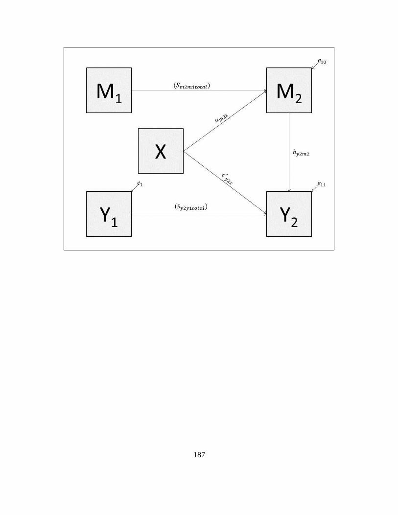
187

188
APPENDIX O
COVARIANCE ALGEBRA

189
𝑋 = 0,1
𝑀1 = 𝑎𝑀1𝑋 ∗ 𝑋 + 𝑒1
𝑌1 = 𝑐𝑌1𝑋 ∗ 𝑋 + 𝑏𝑌1𝑀1 ∗ 𝑀1 + 𝑒2
𝑀2 = 𝑎𝑀2𝑋 ∗ 𝑋 + 𝑠𝑀2𝑀1 ∗ 𝑀1 + 𝑏𝑀2𝑌1 ∗ 𝑌1 + 𝑒3
𝑌2 = 𝑐𝑌2𝑋 ∗ 𝑋 + 𝑠𝑌2𝑌1 ∗ 𝑌1 + 𝑏𝑌2𝑀1 ∗ 𝑀1 + 𝑏𝑌2𝑀2 ∗ 𝑀2 + 𝑒4
𝑇𝑟𝑢𝑒 𝑡𝑜𝑡𝑎𝑙 𝑒𝑓𝑓𝑒𝑐𝑡 𝑜𝑓 𝑋 𝑜𝑛 𝑌2 = (𝑎𝑀2𝑋 ∗ 𝑋) ∗ (𝑏𝑌2𝑀2 ∗ 𝑀2) + (𝑎𝑀1𝑋 ∗ 𝑋) ∗ (𝑠𝑀2𝑀1 ∗
𝑀1) ∗ (𝑏𝑌2𝑀2 ∗ 𝑀2) + (𝑎𝑀1𝑋 ∗ 𝑋) + (𝑏𝑌2𝑀1 ∗ 𝑀1) + (𝑎𝑀1𝑋 ∗ 𝑋) ∗ (𝑏𝑌1𝑀1 ∗ 𝑀1) ∗
(𝑏𝑀2𝑌1 ∗ 𝑌1) ∗ (𝑏𝑌2𝑀2 ∗ 𝑀2) + (𝑐𝑌1𝑋 ∗ 𝑋) ∗ (𝑏𝑀2𝑌1 ∗ 𝑌1) ∗ (𝑏𝑌2𝑀2 ∗ 𝑀2) +
(𝑐𝑌1𝑋 ∗ 𝑋) ∗ (𝑠𝑌2𝑌1 ∗ 𝑌1) + (𝑐𝑌2𝑋 ∗ 𝑋)
𝑪𝒐𝒗(𝑿, 𝑴𝟏) = 𝐶𝑜𝑣(𝑋, 𝑎𝑀1𝑋 ∗ 𝑋 + 𝑒1)
= 𝐶𝑜𝑣(𝑋, 𝑎𝑀1𝑋 ∗ 𝑋) + 𝐶𝑜𝑣(𝑋, 𝑒1)
= 𝑎𝑀1𝑋 ∗ 𝜎𝑋2
𝑪𝒐𝒗(𝑿, 𝒀𝟏) = 𝐶𝑜𝑣(𝑋, 𝑐𝑌1𝑋 ∗ 𝑋 + 𝑏𝑌1𝑀1 ∗ 𝑀1 + 𝑒2)
= 𝐶𝑜𝑣(𝑋, 𝑐𝑌1𝑋 ∗ 𝑋) + 𝐶𝑜𝑣(𝑋, 𝑏𝑌1𝑀1 ∗ 𝑀1) + 𝐶𝑜𝑣(𝑋, 𝑒2)
= 𝑐𝑌1 ∗ 𝜎𝑋2 + 𝑏𝑌1𝑀1 ∗ 𝐶𝑜𝑣(𝑋, 𝑀1)
𝑪𝒐𝒗(𝑿, 𝑴𝟐) = 𝐶𝑜𝑣(𝑋, 𝑎𝑀2𝑋 ∗ 𝑋 + 𝑠𝑀2𝑀1 ∗ 𝑀1 + 𝑏𝑀2𝑌1 ∗ 𝑌1 + 𝑒3)
= 𝐶𝑜𝑣(𝑋, 𝑎𝑀2𝑋 ∗ 𝑋) + 𝐶𝑜𝑣(𝑋, 𝑠𝑀2𝑀1 ∗ 𝑀1) + 𝐶𝑜𝑣(𝑋, 𝑏𝑀2𝑌1 ∗ 𝑌1) + 𝐶𝑜𝑣(𝑋, 𝑒3)
= 𝑎𝑀2𝑋 ∗ 𝜎𝑋2 + 𝑠𝑀2𝑀1 ∗ 𝐶𝑜𝑣(𝑋, 𝑀1) + 𝑏𝑀2𝑌1 ∗ 𝐶𝑜𝑣(𝑋, 𝑌1)
𝑪𝒐𝒗(𝑿, 𝒀𝟐) = 𝐶𝑜𝑣(𝑋, 𝑐𝑌2𝑋 ∗ 𝑋 + 𝑠𝑌2𝑌1 ∗ 𝑌1 + 𝑏𝑌2𝑀1 ∗ 𝑀1 + 𝑏𝑌2𝑀2 ∗ 𝑀2 + 𝑒4)
= 𝐶𝑜𝑣(𝑋, 𝑐𝑌2𝑋 ∗ 𝑋) + 𝐶𝑜𝑣(𝑋, 𝑠𝑌2𝑌1 ∗ 𝑌1) + 𝐶𝑜𝑣(𝑋, 𝑏𝑌2𝑀1 ∗ 𝑀1) + 𝐶𝑜𝑣(𝑋, 𝑏𝑌2𝑀2
∗ 𝑀2) + 𝐶𝑜𝑣(𝑋, 𝑒4)
= 𝑐𝑌2𝑋 ∗ 𝜎𝑋2 + 𝑠𝑌2𝑌1 ∗ 𝐶𝑜𝑣(𝑋, 𝑌1) + 𝑏𝑌2𝑀1 ∗ 𝐶𝑜𝑣(𝑋, 𝑀1) + 𝑏𝑌2𝑀2 ∗ 𝐶𝑜𝑣(𝑋, 𝑀2)

190
𝑪𝒐𝒗(𝑴𝟏, 𝒀𝟏) = 𝐶𝑜𝑣(𝑎𝑀1𝑋 ∗ 𝑋 + 𝑒1, 𝑐𝑌1𝑋 ∗ 𝑋 + 𝑏𝑌1𝑀1 ∗ 𝑀1 + 𝑒2)
= 𝐶𝑜𝑣(𝑎𝑀1𝑋 ∗ 𝑋, 𝑐𝑌1𝑋 ∗ 𝑋) + 𝐶𝑜𝑣(𝑎𝑀1𝑋 ∗ 𝑋, 𝑏𝑌1𝑀1 ∗ 𝑀1) + 𝐶𝑜𝑣(𝑎𝑀1𝑋
∗ 𝑋, 𝑒2) 𝐶𝑜𝑣(𝑒1, 𝑐𝑌1𝑋 ∗ 𝑋) + 𝐶𝑜𝑣(𝑒1, 𝑏𝑌1𝑀1 ∗ 𝑀1) + 𝐶𝑜𝑣(𝑒1, 𝑒2)
= 𝑎𝑀1𝑋 ∗ (𝑐𝑌1𝑋 ∗ 𝜎𝑋2) + 𝑎𝑀1𝑋 ∗ [𝑏𝑌1𝑀1 ∗ 𝐶𝑜𝑣(𝑋, 𝑀1)] + 𝑏𝑌1𝑀1 ∗ 𝜎𝑒1
2
𝑪𝒐𝒗(𝑴𝟏, 𝑴𝟐) = 𝐶𝑜𝑣(𝑎𝑀1𝑋 ∗ 𝑋 + 𝑒1, 𝑠𝑀2𝑀1 ∗ 𝑀1 + 𝑏𝑀2𝑌1 ∗ 𝑌1 + 𝑎𝑀2𝑋 ∗ 𝑋 + 𝑒3)
= 𝐶𝑜𝑣(𝑎𝑀1𝑋 ∗ 𝑋, 𝑠𝑀2𝑀1 ∗ 𝑀1) + 𝐶𝑜𝑣(𝑎𝑀1𝑋 ∗ 𝑋, 𝑏𝑀2𝑌1 ∗ 𝑌1) + 𝐶𝑜𝑣(𝑎𝑀1𝑋 ∗ 𝑋, 𝑎𝑀2𝑋
∗ 𝑋) + 𝐶𝑜𝑣(𝑎𝑀1𝑋 ∗ 𝑋, 𝑒3) + + 𝐶𝑜𝑣(𝑒1, 𝑠𝑀2𝑀1 ∗ 𝑀1) + 𝐶𝑜𝑣(𝑒1, 𝑏𝑀2𝑌1
∗ 𝑌1) + 𝐶𝑜𝑣(𝑒1, 𝑎𝑀2𝑋 ∗ 𝑋) + 𝐶𝑜𝑣(𝑒1, 𝑒3)
= 𝑎𝑀1𝑋 ∗ [𝑠𝑀2𝑀1 ∗ 𝐶𝑜𝑣(𝑋, 𝑀1)] + 𝑎𝑀1𝑋 ∗ [𝑏𝑀2𝑌1 ∗ 𝐶𝑜𝑣(𝑋, 𝑌1)] + 𝑎𝑀1𝑋 ∗ (𝑎𝑀2𝑋
∗ 𝜎𝑋2) + 𝑠𝑀2𝑀1 ∗ 𝜎𝑒1
2 + 𝑏𝑀2𝑌1 ∗ (𝑏𝑌1𝑀1 ∗ 𝜎𝑒12 )
𝑪𝒐𝒗(𝑴𝟏, 𝒀𝟐) = 𝐶𝑜𝑣(𝑎𝑀1𝑋 ∗ 𝑋 + 𝑒1, 𝑐𝑌2𝑋 ∗ 𝑋 + 𝑠𝑌2𝑌1 ∗ 𝑌1 + 𝑏𝑌2𝑀1 ∗ 𝑀1 + 𝑏𝑌2𝑀2
∗ 𝑀2 + 𝑒4)
= 𝐶𝑜𝑣(𝑎𝑀1𝑋 ∗ 𝑋, 𝑐𝑌2𝑋 ∗ 𝑋) + 𝐶𝑜𝑣(𝑎𝑀1𝑋 ∗ 𝑋, 𝑠𝑌2𝑌1 ∗ 𝑌1) + 𝐶𝑜𝑣(𝑎𝑀1𝑋 ∗ 𝑋, 𝑏𝑌2𝑀1
∗ 𝑀1) + 𝐶𝑜𝑣(𝑎𝑀1𝑋 ∗ 𝑋, 𝑏𝑌2𝑀2 ∗ 𝑀2) + 𝐶𝑜𝑣(𝑎𝑀1𝑋 ∗ 𝑋, 𝑒4)
+ 𝐶𝑜𝑣(𝑒1, 𝑐𝑌2𝑋 ∗ 𝑋) + 𝐶𝑜𝑣(𝑒1, 𝑠𝑌2𝑌1 ∗ 𝑌1) + 𝐶𝑜𝑣(𝑒1, 𝑏𝑌2𝑀1 ∗ 𝑀1)
+ 𝐶𝑜𝑣(𝑒1, 𝑏𝑌2𝑀2 ∗ 𝑀2) + 𝐶𝑜𝑣(𝑒1, 𝑒4)
= 𝑎𝑀1𝑋 ∗ (𝑐𝑌2𝑋 ∗ 𝜎𝑋2) + 𝑎𝑀1𝑋 ∗ [𝑠𝑌2𝑌1 ∗ 𝐶𝑜𝑣(𝑋, 𝑌1)] + 𝑎𝑀1𝑋 ∗ [𝑏𝑌2𝑀1
∗ 𝐶𝑜𝑣(𝑋, 𝑀1)] + 𝑎𝑀1𝑋 ∗ [𝑏𝑌2𝑀2 ∗ 𝐶𝑜𝑣(𝑋, 𝑀2)] + 𝑠𝑌2𝑌1 ∗ (𝑏𝑌1𝑀1
∗ 𝜎𝑒12 ) + 𝑏𝑌2𝑀1 ∗ 𝜎𝑒1
2 + 𝑏𝑌2𝑀2 ∗ [(𝑠𝑀2𝑀1 ∗ 𝜎𝑒12 ) + (𝑏𝑀2𝑌1 ∗ 𝑏𝑌1𝑀1
∗ 𝜎𝑒12 )]
𝑪𝒐𝒗 (𝑴𝟐, 𝒀𝟏) = 𝐶𝑜𝑣(𝑎𝑀2𝑋 ∗ 𝑋 + 𝑠𝑀2𝑀1 ∗ 𝑀1 + 𝑏𝑀2𝑌1 ∗ 𝑌1 + 𝑒3, 𝑏𝑌1𝑀1 ∗ 𝑀1
+ 𝑐𝑌1𝑋 ∗ 𝑋 + 𝑒2)
= 𝐶𝑜𝑣(𝑎𝑀2𝑋 ∗ 𝑋, 𝑏𝑌1𝑀1 ∗ 𝑀1) + 𝐶𝑜𝑣(𝑎𝑀2𝑋 ∗ 𝑋, 𝑐𝑌1𝑋 ∗ 𝑋) + 𝐶𝑜𝑣(𝑎𝑀2𝑋 ∗ 𝑋, 𝑒2)
+ 𝐶𝑜𝑣(𝑠𝑀2𝑀1 ∗ 𝑀1, 𝑏𝑌1𝑀1 ∗ 𝑀1) + 𝐶𝑜𝑣(𝑠𝑀2𝑀1 ∗ 𝑀1, 𝑏𝑌1𝑀1 ∗ 𝑀1)
+ 𝐶𝑜𝑣(𝑠𝑀2𝑀1 ∗ 𝑀1, 𝑐𝑌1𝑋 ∗ 𝑋) + 𝐶𝑜𝑣(𝑠𝑀2𝑀1 ∗ 𝑀1, 𝑒2) + 𝐶𝑜𝑣(𝑏𝑀2𝑌1
∗ 𝑌1, 𝑏𝑌1𝑀1 ∗ 𝑀1) + 𝐶𝑜𝑣(𝑏𝑀2𝑌1 ∗ 𝑌1, 𝑐𝑌1𝑋 ∗ 𝑋) + 𝐶𝑜𝑣(𝑏𝑀2𝑌1
∗ 𝑌1, 𝑒2) + 𝐶𝑜𝑣(𝑒3, 𝑏𝑌1𝑀1 ∗ 𝑀1) + +𝐶𝑜𝑣(𝑒3, 𝑐𝑌1𝑋 ∗ 𝑋) + 𝐶𝑜𝑣(𝑒3, 𝑒2)

191
= 𝑎𝑀2𝑋 ∗ [𝑏𝑌1𝑀1 ∗ 𝐶𝑜𝑣(𝑋, 𝑀1)] + 𝑎𝑀2𝑋 ∗ (𝑐𝑌1𝑋 ∗ 𝜎𝑋2) + 𝑠𝑀2𝑀1 ∗ (𝑏𝑌1𝑀1 ∗ 𝜎𝑀1
2 )
+ 𝑠𝑀2𝑀1 ∗ [𝑐𝑌1𝑋 ∗ 𝐶𝑜𝑣(𝑋, 𝑀1)] + 𝑏𝑀2𝑌1 ∗ [𝑏𝑌1𝑀1 ∗ 𝐶𝑜𝑣(𝑌1, 𝑀1)]
+ 𝑏𝑀2𝑌1 ∗ [𝑐𝑌1𝑋 ∗ 𝐶𝑜𝑣(𝑋, 𝑌1)] + 𝑏𝑀2𝑌1 ∗ 𝜎𝑒22
𝑪𝒐𝒗(𝒀𝟏, 𝒀𝟐) = 𝐶𝑜𝑣(𝑐𝑌1𝑋 ∗ 𝑋 + 𝑏𝑌1𝑀1 ∗ 𝑀1 + 𝑒2, 𝑠𝑌2𝑌1 ∗ 𝑌1 + 𝑏𝑌2𝑀1 ∗ 𝑀1
+ 𝑏𝑌2𝑀2 ∗ 𝑀2 + 𝑐𝑌2𝑋 ∗ 𝑋 + 𝑒4)
= 𝐶𝑜𝑣(𝑐𝑌1𝑋 ∗ 𝑋, 𝑠𝑌2𝑌1 ∗ 𝑌1) + 𝐶𝑜𝑣(𝑐𝑌1𝑋 ∗ 𝑋, 𝑏𝑌2𝑀1 ∗ 𝑀1) + 𝐶𝑜𝑣(𝑐𝑌1𝑋 ∗ 𝑋, 𝑏𝑌2𝑀2
∗ 𝑀2) + 𝐶𝑜𝑣(𝑐𝑌1𝑋 ∗ 𝑋, 𝑐𝑌2𝑋 ∗ 𝑋) + 𝐶𝑜𝑣(𝑐𝑌1𝑋 ∗ 𝑋, 𝑒4) + 𝐶𝑜𝑣(𝑏𝑌1𝑀1
∗ 𝑀1, 𝑠𝑌2𝑌1 ∗ 𝑌1) + 𝐶𝑜𝑣(𝑏𝑌1𝑀1 ∗ 𝑀1, 𝑏𝑌2𝑀1 ∗ 𝑀1) + 𝐶𝑜𝑣(𝑏𝑌1𝑀1
∗ 𝑀1, 𝑏𝑌2𝑀2 ∗ 𝑀2) + 𝐶𝑜𝑣(𝑏𝑌1𝑀1 ∗ 𝑀1, 𝑐𝑌2𝑋 ∗ 𝑋) + 𝐶𝑜𝑣(𝑏𝑌1𝑀1
∗ 𝑀1, 𝑒4) + 𝐶𝑜𝑣(𝑒2, 𝑠𝑌2𝑌1 ∗ 𝑌1) + +𝐶𝑜𝑣(𝑒2, 𝑏𝑌2𝑀1 ∗ 𝑀1)
+ 𝐶𝑜𝑣(𝑒2, 𝑏𝑌2𝑀2 ∗ 𝑀2) + 𝐶𝑜𝑣(𝑒2, 𝑐𝑌2𝑋 ∗ 𝑋) + 𝐶𝑜𝑣(𝑒2, 𝑒4)
= 𝑐𝑌1𝑋 ∗ [𝑠𝑌2𝑌1 ∗ 𝐶𝑜𝑣(𝑋, 𝑌1)] + 𝑐𝑌1𝑋 ∗ [𝑏𝑌2𝑀1 ∗ 𝐶𝑜𝑣(𝑋, 𝑀1)] + 𝑐𝑌1𝑋 ∗ [𝑏𝑌2𝑀2
∗ 𝐶𝑜𝑣(𝑋, 𝑀2)] + 𝑐𝑌1𝑋 ∗ (𝑐𝑌2𝑋 ∗ 𝜎𝑋2) + 𝑏𝑌1𝑀1 ∗ [𝑠𝑌2𝑌1 ∗ 𝐶𝑜𝑣(𝑀1, 𝑌1)]
+ 𝑏𝑌1𝑀1 ∗ (𝑏𝑌2𝑀1 ∗ 𝜎𝑀12 ) + 𝑏𝑌1𝑀1 ∗ [𝑏𝑌2𝑀2 ∗ 𝐶𝑜𝑣(𝑀1, 𝑀2)] + 𝑏𝑌1𝑀1
∗ 𝑐𝑌2𝑋 ∗ 𝐶𝑜𝑣(𝑋, 𝑀1) + 𝑏𝑌2𝑀2 ∗ (𝑏𝑀2𝑌1 ∗ 𝜎𝑒22 ) + 𝑠𝑌2𝑌1 ∗ 𝜎𝑒2
2
𝑪𝒐𝒗(𝑴𝟐, 𝒀𝟐) = 𝐶𝑜𝑣(𝑠𝑀2𝑀1 ∗ 𝑀1 + 𝑏𝑀2𝑌1 ∗ 𝑌1 + 𝑎𝑀2𝑋 ∗ 𝑋 + 𝑒3, 𝑐𝑌2𝑋 ∗ 𝑋 + 𝑠𝑌2𝑌1
∗ 𝑌1 + 𝑏𝑌2𝑀1 ∗ 𝑀1 + +𝑏𝑌2𝑀2 ∗ 𝑀2 + 𝑒4)
= 𝐶𝑜𝑣(𝑠𝑀2𝑀1 ∗ 𝑀1, 𝑐𝑌2𝑋 ∗ 𝑋) + 𝐶𝑜𝑣(𝑠𝑀2𝑀1 ∗ 𝑀1, 𝑠𝑌2𝑌1 ∗ 𝑌1) + 𝐶𝑜𝑣(𝑠𝑀2𝑀1
∗ 𝑀1, 𝑏𝑌2𝑀1 ∗ 𝑀1) + +𝐶𝑜𝑣(𝑠𝑀2𝑀1 ∗ 𝑀1, 𝑏𝑌2𝑀2 ∗ 𝑀2) + 𝐶𝑜𝑣(𝑠𝑀2𝑀1
∗ 𝑀1, 𝑒4) + 𝐶𝑜𝑣(𝑏𝑀2𝑌1 ∗ 𝑌1, 𝑐𝑌2𝑋 ∗ 𝑋) + 𝐶𝑜𝑣(𝑏𝑀2𝑌1 ∗ 𝑌1, 𝑠𝑌2𝑌1 ∗ 𝑌1)
+ 𝐶𝑜𝑣(𝑏𝑀2𝑌1 ∗ 𝑌1, 𝑏𝑌2𝑀1 ∗ 𝑀1) + 𝐶𝑜𝑣(𝑏𝑀2𝑌1 ∗ 𝑌1, 𝑏𝑌2𝑀2 ∗ 𝑀2)
+ +𝐶𝑜𝑣(𝑏𝑀2𝑌1 ∗ 𝑌1, 𝑒4) + 𝐶𝑜𝑣(𝑎𝑀2𝑋 ∗ 𝑋, 𝑐𝑌2𝑋 ∗ 𝑋) + 𝐶𝑜𝑣(𝑎𝑀2𝑋
∗ 𝑋, 𝑠𝑌2𝑌1 ∗ 𝑌1) + 𝐶𝑜𝑣(𝑎𝑀2𝑋 ∗ 𝑋, 𝑏𝑌2𝑀1 ∗ 𝑀1) + +𝐶𝑜𝑣(𝑎𝑀2𝑋
∗ 𝑋, 𝑏𝑌2𝑀2 ∗ 𝑀2) + 𝐶𝑜𝑣(𝑒3, 𝑐𝑌2𝑋 ∗ 𝑋) + 𝐶𝑜𝑣(𝑒3, 𝑠𝑌2𝑌1 ∗ 𝑌1)
+ 𝐶𝑜𝑣(𝑒3, 𝑏𝑌2𝑀1 ∗ 𝑀1) + 𝐶𝑜𝑣(𝑒3, 𝑏𝑌2𝑀2 ∗ 𝑀2) + 𝐶𝑜𝑣(𝑒3, 𝑒4)
𝑠𝑀2𝑀1 ∗ 𝑠𝑌2𝑌1 ∗ [𝐶𝑜𝑣(𝑀1, 𝑌1)] + 𝑠𝑀2𝑀1 ∗ (𝑏𝑌2𝑀1 ∗ 𝜎𝑀12 ) + 𝑠𝑀2𝑀1 ∗ [𝑏𝑌2𝑀2
∗ 𝐶𝑜𝑣(𝑀1, 𝑀2)] + 𝑏𝑀2𝑌1 ∗ (𝑠𝑌2𝑌1 ∗ 𝜎𝑌12 ) + 𝑏𝑀2𝑌1 ∗ [𝑏𝑌2𝑀1
∗ 𝐶𝑜𝑣(𝑌1, 𝑀1)] + 𝑏𝑀2𝑌1 ∗ [𝑏𝑌2𝑀2 ∗ 𝐶𝑜𝑣(𝑌1, 𝑀2)] + 𝑎𝑀2𝑋 ∗ (𝑐𝑌2𝑋
∗ 𝜎𝑋2) + 𝑎𝑀2𝑋 ∗ [𝑏𝑌2𝑀2 ∗ 𝐶𝑜𝑣(𝑋, 𝑀2)] + 𝑏𝑌2𝑀2 ∗ 𝜎𝑒3
2
𝑪𝒐𝒗(𝑴𝟏, 𝑴𝟏) = 𝐶𝑜𝑣(𝑎𝑀1𝑋 ∗ 𝑋 + 𝑒1, 𝑎𝑀1𝑋 ∗ 𝑋 + 𝑒1)
192
= 𝐶𝑜𝑣(𝑎𝑀1𝑋 ∗ 𝑋, 𝑎𝑀1𝑋 ∗ 𝑋) + 2 ∗ 𝐶𝑜𝑣(𝑎𝑀1𝑋 ∗ 𝑋, 𝑒1) + 𝐶𝑜𝑣(𝑒1, 𝑒1)
= 𝑎𝑀1𝑋2 ∗ 𝜎𝑋2 + 𝜎𝑒1
2
𝑪𝒐𝒗(𝑴𝟐, 𝑴𝟐) = 𝐶𝑜𝑣(𝑠𝑀2𝑀1 ∗ 𝑀1 + 𝑏𝑀2𝑌1 ∗ 𝑌1 + 𝑎𝑀2𝑋 ∗ 𝑋 + 𝑒3, 𝑠𝑀2𝑀1 ∗ 𝑀1
+ 𝑏𝑀2𝑌1 ∗ 𝑌1 + 𝑎𝑀2𝑋 ∗ 𝑋 + 𝑒3)
= 𝐶𝑜𝑣(𝑠𝑀2𝑀1 ∗ 𝑀1, 𝑠𝑀2𝑀1 ∗ 𝑀1) + 𝐶𝑜𝑣(𝑠𝑀2𝑀1 ∗ 𝑀1, 𝑏𝑀2𝑌1 ∗ 𝑌1) + 𝐶𝑜𝑣(𝑠𝑀2𝑀1
∗ 𝑀1, 𝑎𝑀2𝑋 ∗ 𝑋) + +𝐶𝑜𝑣(𝑠𝑀2𝑀1 ∗ 𝑀1, 𝑒3) + 𝐶𝑜𝑣(𝑏𝑀2𝑌1 ∗ 𝑌1, 𝑠𝑀2𝑀1
∗ 𝑀1) + 𝐶𝑜𝑣(𝑏𝑀2𝑌1 ∗ 𝑌1, 𝑏𝑀2𝑌1 ∗ 𝑌1) + 𝐶𝑜𝑣(𝑏𝑀2𝑌1 ∗ 𝑌1, 𝑎𝑀2𝑋 ∗ 𝑋)
+ 𝐶𝑜𝑣(𝑏𝑀2𝑌1 ∗ 𝑌1, 𝑒3) + 𝐶𝑜𝑣(𝑎𝑀2𝑋 ∗ 𝑋, 𝑠𝑀2𝑀1 ∗ 𝑀1) + 𝐶𝑜𝑣(𝑎𝑀2𝑋
∗ 𝑋, 𝑏𝑀2𝑌1 ∗ 𝑌1) + +𝐶𝑜𝑣(𝑎𝑀2𝑋 ∗ 𝑋, 𝑏𝑀2𝑌1 ∗ 𝑌1) + 𝐶𝑜𝑣(𝑎𝑀2𝑋
∗ 𝑋, 𝑎𝑀2𝑋 ∗ 𝑋) + 𝐶𝑜𝑣(𝑎𝑀2𝑋 ∗ 𝑋, 𝑒3) + +𝐶𝑜𝑣(𝑒3, 𝑠𝑀2𝑀1 ∗ 𝑀1)
+ +𝐶𝑜𝑣(𝑒3, 𝑏𝑀2𝑌1 ∗ 𝑌1) + 𝐶𝑜𝑣(𝑒3, 𝑎𝑀2𝑋 ∗ 𝑋) + 𝐶𝑜𝑣(𝑒3, 𝑒3)
= 𝑠𝑀2𝑀1 ∗ 𝜎𝑀12 + 2 ∗ 𝑠𝑀2𝑀1 ∗ [𝑏𝑀2𝑌1 ∗ 𝐶𝑜𝑣(𝑀1, 𝑌1)] + 2 ∗ 𝑠𝑀2𝑀1 ∗ [𝑎𝑀2𝑋
∗ 𝐶𝑜𝑣(𝑋, 𝑀1)] + 𝑏𝑀2𝑌12 ∗ 𝜎𝑌12 + 2 ∗ 𝑏𝑀2𝑌1 ∗ [𝑎𝑀2𝑋 ∗ 𝐶𝑜𝑣(𝑋, 𝑌1)]
+ 𝑎𝑀2𝑋2 ∗ 𝜎𝑋2 + 𝜎𝑒3
2
𝑪𝒐𝒗(𝒀𝟏, 𝒀𝟏) = 𝐶𝑜𝑣(𝑐𝑌1𝑋 ∗ 𝑋 + 𝑏𝑌1𝑀1 ∗ 𝑀1 + 𝑒2, 𝑐𝑌1𝑋 ∗ 𝑋 + 𝑏𝑌1𝑀1 ∗ 𝑀1 + 𝑒2)
= 𝐶𝑜𝑣(𝑐𝑌1𝑋 ∗ 𝑋, 𝑐𝑌1𝑋 ∗ 𝑋) + 𝐶𝑜𝑣(𝑐𝑌1𝑋 ∗ 𝑋, 𝑏𝑌1𝑀1 ∗ 𝑀1) + 𝐶𝑜𝑣(𝑐𝑌1𝑋 ∗ 𝑋, 𝑒2)
+ 𝐶𝑜𝑣(𝑏𝑌1𝑀1 ∗ 𝑀1, 𝑐𝑌1𝑋 ∗ 𝑋) + +𝐶𝑜𝑣(𝑏𝑌1𝑀1 ∗ 𝑀1, 𝑏𝑌1𝑀1 ∗ 𝑀1)
+ 𝐶𝑜𝑣(𝑏𝑌1𝑀1 ∗ 𝑀1, 𝑒2) + 𝐶𝑜𝑣(𝑒2, 𝑐𝑌1𝑋 ∗ 𝑋) + 𝐶𝑜𝑣(𝑒2, 𝑏𝑌1𝑀1 ∗ 𝑀1)
+ +𝐶𝑜𝑣(𝑒2, 𝑒2)
= 𝑐𝑌1𝑋2 ∗ 𝜎𝑋2 + 2 ∗ 𝑐𝑌1𝑋 ∗ [𝑏𝑌1𝑀1 ∗ 𝐶𝑜𝑣(𝑋, 𝑀1)] + 𝑏𝑌1𝑀12 ∗ 𝜎𝑀1
2 + 𝜎𝑒22
𝑪𝒐𝒗(𝒀𝟐, 𝒀𝟐) = 𝐶𝑜𝑣(𝑐𝑌2𝑋 ∗ 𝑋 + 𝑠𝑌2𝑌1 ∗ 𝑌1 + 𝑏𝑌2𝑀1 ∗ 𝑀1 + 𝑏𝑌2𝑀2 ∗ 𝑀2 + 𝑒4, 𝑐𝑌2𝑋
∗ 𝑋 + 𝑠𝑌2𝑌1 ∗ 𝑌1 + 𝑏𝑌2𝑀1 ∗ 𝑀1 + 𝑏𝑌2𝑀2 ∗ 𝑀2 + 𝑒4)
193
= 𝐶𝑜𝑣(𝑐𝑌2𝑋 ∗ 𝑋, 𝑐𝑌2𝑋 ∗ 𝑋) + 𝐶𝑜𝑣(𝑐𝑌2𝑋 ∗ 𝑋, 𝑠𝑌2𝑌1 ∗ 𝑌1) + 𝐶𝑜𝑣(𝑐𝑌2𝑋 ∗ 𝑋, 𝑏𝑌2𝑀1
∗ 𝑀1) + 𝐶𝑜𝑣(𝑐𝑌2𝑋 ∗ 𝑋, 𝑏𝑌2𝑀2 ∗ 𝑀2) + 𝐶𝑜𝑣(𝑐𝑌2𝑋 ∗ 𝑋, 𝑒4) + 𝐶𝑜𝑣(𝑠𝑌2𝑌1
∗ 𝑌1, 𝑐𝑌2𝑋 ∗ 𝑋) + 𝐶𝑜𝑣(𝑠𝑌2𝑌1 ∗ 𝑌1, 𝑠𝑌2𝑌1 ∗ 𝑌1) + 𝐶𝑜𝑣(𝑠𝑌2𝑌1
∗ 𝑌1, 𝑏𝑌2𝑀1 ∗ 𝑀1) + +𝐶𝑜𝑣(𝑠𝑌2𝑌1 ∗ 𝑌1, 𝑏𝑌2𝑀2 ∗ 𝑀2) + 𝐶𝑜𝑣(𝑠𝑌2𝑌1
∗ 𝑌1, 𝑒4) + 𝐶𝑜𝑣(𝑏𝑌2𝑀1 ∗ 𝑀1, 𝑐𝑌2𝑋 ∗ 𝑋) + 𝐶𝑜𝑣(𝑏𝑌2𝑀1 ∗ 𝑀1, 𝑠𝑌2𝑌1 ∗ 𝑌1)
+ 𝐶𝑜𝑣(𝑏𝑌2𝑀1 ∗ 𝑀1, 𝑏𝑌2𝑀1 ∗ 𝑀1) + 𝐶𝑜𝑣(𝑏𝑌2𝑀1 ∗ 𝑀1, 𝑏𝑌2𝑀2 ∗ 𝑀2)
+ +𝐶𝑜𝑣(𝑏𝑌2𝑀1 ∗ 𝑀1, 𝑒4) + 𝐶𝑜𝑣(𝑏𝑌2𝑀2 ∗ 𝑀2, 𝑐𝑌2𝑋 ∗ 𝑋) + 𝐶𝑜𝑣(𝑏𝑌2𝑀2
∗ 𝑀2, 𝑠𝑌2𝑌1 ∗ 𝑌1) + 𝐶𝑜𝑣(𝑏𝑌2𝑀2 ∗ 𝑀2, 𝑏𝑌2𝑀1 ∗ 𝑀1) + 𝐶𝑜𝑣(𝑏𝑌2𝑀2
∗ 𝑀2, 𝑏𝑌2𝑀2 ∗ 𝑀2) + 𝐶𝑜𝑣(𝑏𝑌2𝑀2 ∗ 𝑀2, 𝑒4) + 𝐶𝑜𝑣(𝑒4, 𝑐𝑌2𝑋 ∗ 𝑋)
+ 𝐶𝑜𝑣(𝑒4, 𝑠𝑌2𝑌1 ∗ 𝑌1) + 𝐶𝑜𝑣(𝑒4, 𝑏𝑌2𝑀1 ∗ 𝑀1) + 𝐶𝑜𝑣(𝑒4, 𝑏𝑌2𝑀2 ∗ 𝑀2)
+ 𝐶𝑜𝑣(𝑒4, 𝑒4)
= 𝑐𝑌2𝑋2 ∗ 𝜎𝑋2 + 2 ∗ 𝑐𝑌2𝑋 ∗ [𝑠𝑌2𝑌1 ∗ 𝐶𝑜𝑣(𝑋, 𝑌1)] + 2 ∗ 𝑐𝑌2𝑋 ∗ [𝑏𝑌2𝑀1 ∗ 𝐶𝑜𝑣(𝑋, 𝑀1)]
+ 2 ∗ 𝑐𝑌2𝑋 ∗ [𝑏𝑌2𝑀2 ∗ 𝐶𝑜𝑣(𝑋, 𝑀2)] + 𝑠𝑌2𝑌1 ∗ 𝜎𝑌12 + 2 ∗ 𝑠𝑌2𝑌1 ∗ [𝑏𝑌2𝑀1
∗ 𝐶𝑜𝑣(𝑌1, 𝑀1)] + 2 ∗ 𝑠𝑌2𝑌1 ∗ [𝑏𝑌2𝑀2 ∗ 𝐶𝑜𝑣(𝑌1, 𝑀2)] + 𝑏𝑌2𝑀1 ∗ 𝜎𝑀12 + 2
∗ 𝑏𝑌2𝑀1 ∗ [𝑏𝑌2𝑀2 ∗ 𝐶𝑜𝑣(𝑀1, 𝑀2)] + 𝑏𝑌2𝑀2 ∗ 𝜎𝑀22 + 𝜎𝑒4
2
𝑪𝒐𝒗[(𝑴𝟐 − 𝑴𝟏), (𝑴𝟐 − 𝑴𝟏)] = 𝑉𝐴𝑅(𝑀2) + 𝑉𝐴𝑅(𝑀1) – 2 ∗ 𝐶𝑜𝑣(𝑀1, 𝑀2)
𝑪𝒐𝒗[(𝒀𝟐 − 𝒀𝟏), (𝒀𝟐 − 𝒀𝟏)] = 𝑉𝐴𝑅(𝑌2) + 𝑉𝐴𝑅(𝑌1) – 2 ∗ 𝐶𝑜𝑣(𝑌1, 𝑌2)
𝑪𝒐𝒗[𝑿, (𝒀𝟐 − 𝒀𝟏)]
= 𝐶𝑜𝑣[𝑋, (𝑐𝑌2𝑋 ∗ 𝑋 + 𝑆𝑌2𝑌1 ∗ 𝑌1 + 𝑏𝑌2𝑀1 ∗ 𝑀1 + 𝑏𝑌2𝑀2 ∗ 𝑀2 + 𝑒4)
− (𝑐𝑌1𝑋 ∗ 𝑋 + 𝑏𝑌1𝑀1 ∗ 𝑀1 + 𝑒2)]
= 𝐶𝑜𝑣[𝑋, (𝑐𝑌2𝑋 − 𝑐𝑌1𝑋) ∗ 𝑋 + 𝑆𝑌2𝑌1 ∗ 𝑌1 + (𝑏𝑌2𝑀1 − 𝑏𝑌1𝑀1) ∗ 𝑀1 + 𝑏𝑌2𝑀2 ∗ 𝑀2
+ 𝑒4 − 𝑒2]
= 𝐶𝑜𝑣[𝑋, (𝑐𝑌2𝑋 − 𝑐𝑌1𝑋) ∗ 𝑋] + 𝐶𝑜𝑣[𝑋, 𝑆𝑌2𝑌1 ∗ 𝑌1] + 𝐶𝑜𝑣[𝑋, (𝑏𝑌2𝑀1 − 𝑏𝑌1𝑀1) ∗ 𝑀1]
+ 𝐶𝑜𝑣[𝑋, 𝑏𝑌2𝑀2 ∗ 𝑀2] + 𝐶𝑜𝑣[𝑋, 𝑒4] + 𝐶𝑜𝑣[𝑋, −𝑒2]
= (𝑐𝑌2𝑋 − 𝑐𝑌1𝑋) ∗ 𝜎𝑋2 + 𝑆𝑌2𝑌1 ∗ 𝐶𝑜𝑣(𝑋, 𝑌1) + (𝑏𝑌2𝑀1 − 𝑏𝑌1𝑀1) ∗ 𝐶𝑜𝑣(𝑋, 𝑀1)
+ 𝑏𝑌2𝑀2 ∗ 𝐶𝑜𝑣(𝑋, 𝑀2)
𝑪𝒐𝒗[𝑿, (𝑴𝟐 − 𝑴𝟏)]
= 𝐶𝑜𝑣[𝑋, (𝑎𝑀2𝑋 ∗ 𝑋 + 𝑆𝑀2𝑀1 ∗ 𝑀1 + 𝑏𝑀2𝑌1 ∗ 𝑌1 + 𝑒3) – (𝑎𝑀1𝑋 ∗ 𝑋
+ 𝑒1)]

194
= 𝐶𝑜𝑣[𝑋, (𝑎𝑀2𝑋 − 𝑎𝑀1𝑋) ∗ 𝑋 + 𝑆𝑀2𝑀1 ∗ 𝑀1 + 𝑏𝑀2𝑌1 ∗ 𝑌1 + 𝑒3 − 𝑒1]
= 𝐶𝑜𝑣[𝑋, (𝑎𝑀2𝑋 − 𝑎𝑀1𝑋) ∗ 𝑋] + 𝐶𝑜𝑣[𝑋, 𝑆𝑀2𝑀1 ∗ 𝑀1] + 𝐶𝑜𝑣[𝑋, 𝑏𝑀2𝑌1 ∗ 𝑌1]
+ 𝐶𝑜𝑣[𝑋, 𝑒3] + 𝐶𝑜𝑣[𝑋, −𝑒1]
= (𝑎𝑀2𝑋 − 𝑎𝑀1𝑋) ∗ 𝜎𝑋2 + 𝑆𝑀2𝑀1 ∗ 𝐶𝑜𝑣(𝑋, 𝑀1) + 𝑏𝑀2𝑌1 ∗ 𝐶𝑜𝑣(𝑋, 𝑌1)
𝑪𝒐𝒗[(𝑴𝟐 − 𝑴𝟏), (𝒀𝟐 − 𝒀𝟏)]
= 𝐶𝑜𝑣[(𝑎𝑀2𝑋 − 𝑎𝑀1𝑋) ∗ 𝑋 + 𝑆𝑀2𝑀1 ∗ 𝑀1 + 𝑏𝑀2𝑌1 ∗ 𝑌1 + 𝑒3
− 𝑒1, (𝑐𝑌2𝑋 − 𝑐𝑌1𝑋) ∗ 𝑋 + 𝑆𝑌2𝑌1 ∗ 𝑌1 + (𝑏𝑌2𝑀1 − 𝑏𝑌1𝑀1) ∗ 𝑀1
+ 𝑏𝑌2𝑀2 ∗ 𝑀2 + 𝑒4 – 𝑒2]
= 𝐶𝑜𝑣[(𝑎𝑀2𝑋 − 𝑎𝑀1𝑋) ∗ 𝑋, (𝑐𝑌2𝑋 − 𝑐𝑌1𝑋) ∗ 𝑋] + 𝐶𝑜𝑣[(𝑎𝑀2𝑋 − 𝑎𝑀1𝑋) ∗ 𝑋, 𝑆𝑌2𝑌1
∗ 𝑌1] + 𝐶𝑜𝑣[(𝑎𝑀2𝑋 − 𝑎𝑀1𝑋) ∗ 𝑋, (𝑏𝑌2𝑀1 − 𝑏𝑌1𝑀1) ∗ 𝑀1]
+ 𝐶𝑜𝑣[(𝑎𝑀2𝑋 − 𝑎𝑀1𝑋) ∗ 𝑋, 𝑏𝑌2𝑀2 ∗ 𝑀2] + 𝐶𝑜𝑣[(𝑎𝑀2𝑋 − 𝑎𝑀1𝑋)
∗ 𝑋, 𝑒4] + 𝐶𝑜𝑣[(𝑎𝑀2𝑋 − 𝑎𝑀1𝑋) ∗ 𝑋, −𝑒2] + 𝐶𝑜𝑣[𝑆𝑀2𝑀1 ∗ 𝑀1, (𝑐𝑌2𝑋
− 𝑐𝑌1𝑋) ∗ 𝑋] + 𝐶𝑜𝑣[𝑆𝑀2𝑀1 ∗ 𝑀1, 𝑆𝑌2𝑌1 ∗ 𝑌1] + 𝐶𝑜𝑣[𝑆𝑀2𝑀1
∗ 𝑀1, (𝑏𝑌2𝑀1 − 𝑏𝑌1𝑀1) ∗ 𝑀1] + 𝐶𝑜𝑣[𝑆𝑀2𝑀1 ∗ 𝑀1, 𝑏𝑌2𝑀2 ∗ 𝑀2]
+ 𝐶𝑜𝑣[𝑆𝑀2𝑀1 ∗ 𝑀1, 𝑒4] + 𝐶𝑜𝑣[𝑆𝑀2𝑀1 ∗ 𝑀1, −𝑒2] + 𝐶𝑜𝑣[𝑏𝑀2𝑌1
∗ 𝑌1, (𝑐𝑌2𝑋 − 𝑐𝑌1𝑋) ∗ 𝑋] + 𝐶𝑜𝑣[𝑏𝑀2𝑌1 ∗ 𝑌1, 𝑆𝑌2𝑌1 ∗ 𝑌1] + 𝐶𝑜𝑣[𝑏𝑀2𝑌1
∗ 𝑌1, (𝑏𝑌2𝑀1 − 𝑏𝑌1𝑀1) ∗ 𝑀1] + 𝐶𝑜𝑣[𝑏𝑀2𝑌1 ∗ 𝑌1, 𝑏𝑌2𝑀2 ∗ 𝑀2]
+ 𝐶𝑜𝑣[𝑏𝑀2𝑌1 ∗ 𝑌1, 𝑒4] + 𝐶𝑜𝑣[𝑏𝑀2𝑌1 ∗ 𝑌1, −𝑒2] + 𝐶𝑜𝑣[𝑒3, (𝑐𝑌2𝑋
− 𝑐𝑌1𝑋) ∗ 𝑋] + 𝐶𝑜𝑣[𝑒3, (𝑐𝑌2𝑋 − 𝑐𝑌1𝑋) ∗ 𝑋] + 𝐶𝑜𝑣[𝑒3, 𝑆𝑌2𝑌1 ∗ 𝑌1]
+ 𝐶𝑜𝑣[𝑒3, (𝑏𝑌2𝑀1 − 𝑏𝑌1𝑀1) ∗ 𝑀1] + 𝐶𝑜𝑣[𝑒3, 𝑏𝑌2𝑀2 ∗ 𝑀2]
+ 𝐶𝑜𝑣[𝑒3, 𝑒4] + 𝐶𝑜𝑣[𝑒3, −𝑒2] + 𝐶𝑜𝑣[−𝑒1, (𝑐𝑌2𝑋 − 𝑐𝑌1𝑋) ∗ 𝑋]
+ 𝐶𝑜𝑣[−𝑒1, 𝑆𝑌2𝑌1 ∗ 𝑌1] + 𝐶𝑜𝑣[−𝑒1,
(𝑏𝑌2𝑀1 − 𝑏𝑌1𝑀1) ∗ 𝑀1] + 𝐶𝑜𝑣[−𝑒1, 𝑏𝑌2𝑀2 ∗ 𝑀2] + 𝐶𝑜𝑣[−𝑒1, 𝑒4]
+ 𝐶𝑜𝑣[−𝑒1, −𝑒2]
= (𝑎𝑀2𝑋 − 𝑎𝑀1𝑋) ∗ (𝑐𝑌2𝑋 − 𝑐𝑌1𝑋) ∗ 𝜎𝑋2 + (𝑎𝑀2𝑋 − 𝑎𝑀1𝑋) ∗ 𝐶𝑜𝑣(𝑋, 𝑌1) + (𝑎𝑀2𝑋
− 𝑎𝑀1𝑋) ∗ (𝑏𝑌2𝑀1 − 𝑏𝑌1𝑀1) ∗ 𝐶𝑜𝑣(𝑋, 𝑀1) + (𝑎𝑀2𝑋 − 𝑎𝑀1𝑋) ∗ 𝑏𝑌2𝑀2
∗ 𝐶𝑜𝑣(𝑋, 𝑀2) + 𝑆𝑀2𝑀1 ∗ (𝑐𝑌2𝑋 − 𝑐𝑌1𝑋) ∗ 𝐶𝑜𝑣(𝑋, 𝑀1) + 𝑆𝑀2𝑀1
∗ 𝑆𝑌2𝑌1 ∗ 𝐶𝑜𝑣(𝑀1, 𝑌1) + 𝑆𝑀2𝑀1 ∗ (𝑏𝑌2𝑀1 − 𝑏𝑌1𝑀1) ∗ 𝜎𝑀12 + 𝑆𝑀2𝑀1
∗ 𝑏𝑌2𝑀2 ∗ 𝐶𝑜𝑣(𝑀1, 𝑀2) + 𝑏𝑀2𝑌1 ∗ (𝑐𝑌2𝑋 − 𝑐𝑌1𝑋) ∗ 𝐶𝑜𝑣(𝑋, 𝑌1)
+ 𝑏𝑀2𝑌1 ∗ 𝑆𝑌2𝑌1 ∗ 𝜎𝑌12 + 𝑏𝑀2𝑌1 ∗ (𝑏𝑌2𝑀1 − 𝑏𝑌1𝑀1) ∗ 𝐶𝑜𝑣(𝑀1, 𝑌1)
+ 𝑏𝑀2𝑌1 ∗ 𝑏𝑌2𝑀2 ∗ 𝐶𝑜𝑣(𝑌1, 𝑀2) – 𝑏𝑀2𝑌1 ∗ 𝐶𝑜𝑣(𝑌1, 𝑒2) + 𝑏𝑌2𝑀2
∗ 𝐶𝑜𝑣(𝑀2, 𝑒3) – 𝑆𝑌2𝑌1 ∗ 𝐶𝑜𝑣(𝑌1, 𝑒1) – (𝑏𝑌2𝑀1 − 𝑏𝑌1𝑀1)
∗ 𝐶𝑜𝑣(𝑀1, 𝑒1) – 𝑏𝑌2𝑀2 ∗ 𝐶𝑜𝑣(𝑀2, 𝑒1)

195
𝑪𝒐𝒗(𝒀𝟏, 𝒆𝟐) = 𝐶𝑜𝑣(𝑐𝑌1𝑋 ∗ 𝑋 + 𝑏𝑌1𝑀1 ∗ 𝑀1 + 𝑒2, 𝑒2)
= 𝐶𝑜𝑣(𝑐𝑌1𝑋 ∗ 𝑋, 𝑒2) + 𝐶𝑜𝑣(𝑏𝑌1𝑀1 ∗ 𝑚1, 𝑒2) + 𝐶𝑜𝑣(𝑒2, 𝑒2)
= 𝜎𝑒22
𝑪𝒐𝒗(𝑴𝟐, 𝒆𝟑) = 𝐶𝑜𝑣(𝑎𝑀2𝑋 ∗ 𝑋 + 𝑆𝑀2𝑀1 ∗ 𝑀1 + 𝑆𝑀2𝑌1 ∗ 𝑌1 + 𝑒3, 𝑒3)
= 𝐶𝑜𝑣(𝑎𝑀2𝑋 ∗ 𝑋, 𝑒3) + 𝐶𝑜𝑣(𝑆𝑀2𝑀1 ∗ 𝑀1, 𝑒3) + 𝐶𝑜𝑣(𝑏𝑀2𝑌1 ∗ 𝑌1, 𝑒3) + 𝐶𝑜𝑣(𝑒3, 𝑒3)
= 𝜎𝑒32
𝑪𝒐𝒗(𝒀𝟏, 𝒆𝟏) = 𝐶𝑜𝑣(𝑐𝑌1𝑋 ∗ 𝑋 + 𝑏𝑌1𝑀1 ∗ 𝑀1 + 𝑒2, 𝑒1)
= 𝐶𝑜𝑣(𝑐𝑌1𝑋 ∗ 𝑋, 𝑒1) + 𝐶𝑜𝑣(𝑏𝑌1𝑀1 ∗ 𝑀1, 𝑒1) + 𝐶𝑜𝑣(𝑒2, 𝑒1)
= 𝑏𝑌1𝑀1 ∗ 𝐶𝑜𝑣(𝑀1, 𝑒1)
𝑪𝒐𝒗(𝑴𝟏, 𝒆𝟏) = 𝐶𝑜𝑣(𝑎𝑀1𝑋 ∗ 𝑋 + 𝑒1, 𝑒1)
= 𝐶𝑜𝑣(𝑎𝑀1𝑋 ∗ 𝑋, 𝑒1) + 𝐶𝑜𝑣(𝑒1, 𝑒1)
= 𝜎𝑒12
𝑪𝒐𝒗(𝑴𝟐, 𝒆𝟏) = 𝐶𝑜𝑣(𝑎𝑀2𝑋 ∗ 𝑋 + 𝑆𝑀2𝑀1 ∗ 𝑀1 + 𝑏𝑀2𝑌1 ∗ 𝑌1 + 𝑒3, 𝑒1)
= 𝐶𝑜𝑣(𝑎𝑀2𝑋 ∗ 𝑋, 𝑒1) = 𝐶𝑜𝑣(𝑆𝑀2𝑀1 ∗ 𝑀1, 𝑒1) + 𝐶𝑜𝑣(𝑏𝑀2𝑌1 ∗ 𝑌1, 𝑒1) + 𝐶𝑜𝑣(𝑒3, 𝑒1)
= 𝑆𝑀2𝑀1 ∗ 𝐶𝑜𝑣(𝑀1, 𝑒1) + 𝑏𝑀2𝑌1 ∗ 𝐶𝑜𝑣(𝑌1, 𝑒1)
= 𝑆𝑀2𝑀1 ∗ 𝜎𝑒12 + 𝑏𝑀2𝑌1 ∗ 𝑏𝑌1𝑀1 ∗ 𝜎𝑒1
2
𝒀�̂� = SY2Y1 ∗ Y1
𝑹𝒆𝒔 𝜟𝒀 = 𝑌2 − 𝑌2̂

196
= 𝑐𝑌2𝑋 ∗ 𝑋 + 𝑆𝑌2𝑌1 ∗ 𝑌1 + 𝑏𝑌2𝑀1 ∗ 𝑀1 + 𝑏𝑌2𝑀2 ∗ 𝑀2 + 𝑒4 − 𝑆𝑌2𝑌1 ∗ 𝑌1
= 𝑐𝑌2𝑋 ∗ 𝑋 + 𝑏𝑌2𝑀1 ∗ 𝑀1 + 𝑏𝑌2𝑀2 ∗ 𝑀2 + 𝑒4
𝑴�̂� = SM2M1 ∗ M1
𝑹𝒆𝒔 𝜟𝑴 = 𝑀2 − 𝑀2̂
= 𝑎𝑀2𝑋 ∗ 𝑋 + 𝑆𝑀2𝑀1 ∗ 𝑀1 + 𝑏𝑀2𝑌1 ∗ 𝑌1 + 𝑒3 − 𝑆𝑀2𝑀1 ∗ 𝑀1
= 𝑎𝑀2𝑋 ∗ 𝑋 + 𝑏𝑀2𝑌1 ∗ 𝑌1 + 𝑒3
𝑪𝒐𝒗(𝑹𝒆𝒔𝜟𝑴, 𝑹𝒆𝒔𝜟𝑴)
= 𝐶𝑜𝑣(𝑎𝑀2𝑋 ∗ 𝑋 + 𝑏𝑀2𝑌1 ∗ 𝑌1 + 𝑒3, 𝑎𝑀2𝑋 ∗ 𝑋 + 𝑏𝑀2𝑌1 ∗ 𝑌1 + 𝑒3)
= 𝐶𝑜𝑣(𝑎𝑀2𝑋 ∗ 𝑋, 𝑎𝑀2𝑋 ∗ 𝑋) + 𝐶𝑜𝑣(𝑎𝑀2𝑋 ∗ 𝑋, 𝑏𝑀2𝑌1 ∗ 𝑌1) + 𝐶𝑜𝑣(𝑎𝑀2𝑋 ∗ 𝑋, 𝑒3)
+ 𝐶𝑜𝑣(𝑏𝑀2𝑌1 ∗ 𝑌1, 𝑎𝑀2𝑋 ∗ 𝑋) + 𝐶𝑜𝑣(𝑏𝑀2𝑌1 ∗ 𝑌1, 𝑏𝑀2𝑌1 ∗ 𝑌1)
+ 𝐶𝑜𝑣(𝑏𝑀2𝑌1 ∗ 𝑌1, 𝑒3) + 𝐶𝑜𝑣(𝑒3, 𝑎𝑀2𝑋 ∗ 𝑋) + 𝐶𝑜𝑣(𝑒3, 𝑏𝑀2𝑌1 ∗ 𝑌1)
+ 𝐶𝑜𝑣(𝑒3, 𝑒3)
= 𝑎𝑀2𝑋2 ∗ 𝜎𝑋2 + 2 ∗ 𝑎𝑀2𝑋 ∗ 𝑏𝑀2𝑌1 ∗ 𝐶𝑜𝑣(𝑋, 𝑌1) + 𝑏𝑀2𝑌12 ∗ 𝜎𝑌1
2 + 𝜎𝑒32
𝑪𝒐𝒗(𝑹𝒆𝒔𝜟𝒀, 𝑹𝒆𝒔𝜟𝒀)
= 𝐶𝑜𝑣(𝑐𝑌2𝑋 ∗ 𝑋 + 𝑏𝑌2𝑀1 ∗ 𝑀1 + 𝑏𝑌2𝑀2 ∗ 𝑀2 + 𝑒4, 𝑐𝑌2𝑋 ∗ 𝑋 + 𝑏𝑌2𝑀1
∗ 𝑀1 + 𝑏𝑌2𝑀2 ∗ 𝑀2 + 𝑒4)
= 𝐶𝑜𝑣(𝑐𝑌2𝑋 ∗ 𝑋, 𝑐𝑌2𝑋 ∗ 𝑋) + 𝐶𝑜𝑣(𝑐𝑌2𝑋 ∗ 𝑋, 𝑏𝑌2𝑀1 ∗ 𝑀1) + 𝐶𝑜𝑣(𝑐𝑌2𝑋 ∗ 𝑋, 𝑏𝑌2𝑀2 ∗ 𝑀2)
+ 𝐶𝑜𝑣(𝑐𝑌2𝑋 ∗ 𝑋, 𝑒4) + 𝐶𝑜𝑣(𝑏𝑌2𝑀1 ∗ 𝑀1, 𝑐𝑌2𝑋 ∗ 𝑋)
+ 𝐶𝑜𝑣(𝑏𝑌2𝑀1 ∗ 𝑀1, 𝑏𝑌2𝑀1 ∗ 𝑀1) + 𝐶𝑜𝑣(𝑏𝑌2𝑀1 ∗ 𝑀1, 𝑏𝑌2𝑀2 ∗ 𝑀2)
+ 𝐶𝑜𝑣(𝑏𝑌2𝑀1 ∗ 𝑀1, 𝑒4) + 𝐶𝑜𝑣(𝑏𝑌2𝑀2 ∗ 𝑀2, 𝑐𝑌2𝑋 ∗ 𝑋)
+ 𝐶𝑜𝑣(𝑏𝑌2𝑀2 ∗ 𝑀2, 𝑏𝑌2𝑀1 ∗ 𝑀1) + 𝐶𝑜𝑣(𝑏𝑌2𝑀2 ∗ 𝑀2, 𝑏𝑌2𝑀2 ∗ 𝑀2)
+ 𝐶𝑜𝑣(𝑏𝑌2𝑀2 ∗ 𝑀2, 𝑒4) + 𝐶𝑜𝑣(𝑒4, 𝑐𝑌2𝑋 ∗ 𝑋) + 𝐶𝑜𝑣(𝑒4, 𝑏𝑌2𝑀1 ∗ 𝑀1)
+ 𝐶𝑜𝑣(𝑒4, 𝑏𝑌2𝑀2 ∗ 𝑀2) + 𝐶𝑜𝑣(𝑒4, 𝑒4)
= 𝑐𝑌2𝑋2 ∗ 𝜎𝑋2 + 𝑐𝑌2𝑋 ∗ 𝑏𝑌2𝑀1 ∗ 𝐶𝑋𝑀1 + 𝑐𝑌2𝑋 ∗ 𝑏𝑌2𝑀2 ∗ 𝐶𝑋𝑀2 + 𝑏𝑌2𝑀1 ∗ 𝑐𝑌2𝑋 ∗ 𝐶𝑋𝑀1
+ 𝑏𝑌2𝑀12 ∗ 𝜎𝑀12 + 𝑏𝑌2𝑀1 ∗ 𝑏𝑌2𝑀2 ∗ 𝐶𝑀1𝑀2 + 𝑏𝑌2𝑀2 ∗ 𝑐𝑌2𝑋 ∗ 𝐶𝑋𝑀2
+ 𝑏𝑌2𝑀2 ∗ 𝑏𝑌2𝑀1 ∗ 𝐶𝑀1𝑀2 + 𝑏𝑌2𝑀22 ∗ 𝜎𝑀22 + 𝜎𝑒4
2
𝑪𝒐𝒗(𝑿, 𝑹𝒆𝒔𝜟𝑴) = 𝐶𝑜𝑣(𝑎𝑀2𝑋 ∗ 𝑋 + 𝑏𝑀2𝑌1 ∗ 𝑌1 + 𝑒3)

197
= 𝑎𝑀2𝑋 ∗ 𝜎𝑋2 + 𝑏𝑀2𝑌1 ∗ 𝐶𝑜𝑣(𝑋, 𝑌1)
𝑪𝒐𝒗(𝑹𝒆𝒔𝜟𝑴, 𝑹𝒆𝒔𝜟𝒀)
= 𝐶𝑜𝑣(𝑎𝑀2𝑋 ∗ 𝑋 + 𝑏𝑀2𝑌1 ∗ 𝑌1 + 𝑒3, 𝑐𝑌2𝑋 ∗ 𝑋 + 𝑏𝑌2𝑀1 ∗ 𝑀1 + 𝑏𝑌2𝑀2
∗ 𝑀2 + 𝑒4)
= 𝐶𝑜𝑣(𝑎𝑀2𝑋 ∗ 𝑋, 𝑐𝑌2𝑋 ∗ 𝑋) + 𝐶𝑜𝑣(𝑎𝑀2𝑋 ∗ 𝑋, 𝑏𝑌2𝑀1 ∗ 𝑀1)
+ 𝐶𝑜𝑣(𝑎𝑀2𝑋 ∗ 𝑋, 𝑏𝑌2𝑀2 ∗ 𝑀2) + 𝐶𝑜𝑣(𝑎𝑀2𝑋 ∗ 𝑋, 𝑒4)
+ 𝐶𝑜𝑣(𝑏𝑀2𝑌1 ∗ 𝑌1, 𝑐𝑌2𝑋 ∗ 𝑋) + 𝐶𝑜𝑣(𝑏𝑀2𝑌1 ∗ 𝑌1, 𝑏𝑌2𝑀1 ∗ 𝑀1)
+ 𝐶𝑜𝑣(𝑏𝑀2𝑌1 ∗ 𝑌1, 𝑏𝑌2𝑀2 ∗ 𝑀2) + 𝐶𝑜𝑣(𝑏𝑀2𝑌1 ∗ 𝑌1, 𝑒4)
+ 𝐶𝑜𝑣(𝑒3, 𝑐𝑌2𝑋 ∗ 𝑋) + 𝐶𝑜𝑣(𝑒3, 𝑏𝑌2𝑀1 ∗ 𝑀1) + 𝐶𝑜𝑣(𝑒3, 𝑏𝑌2𝑀2 ∗ 𝑀2)
+ 𝐶𝑜𝑣(𝑒3, 𝑒4)
= 𝑎𝑀2𝑋 ∗ 𝑐𝑌2𝑋 ∗ 𝜎𝑋2 + 𝑎𝑀2𝑋 ∗ 𝑏𝑌2𝑀1 ∗ 𝐶𝑜𝑣(𝑋, 𝑀1) + 𝑎𝑀2𝑋 ∗ 𝑏𝑌2𝑀2 ∗ 𝐶𝑜𝑣(𝑋, 𝑀2)
+ 𝑏𝑀2𝑌1 ∗ 𝑐𝑌2𝑋 ∗ 𝐶𝑜𝑣(𝑋, 𝑌1) + 𝑏𝑀2𝑌1 ∗ 𝑏𝑌2𝑀1 ∗ 𝐶𝑜𝑣(𝑀1, 𝑌1) + 𝑏𝑀2𝑌1
∗ 𝑏𝑌2𝑀2 ∗ 𝐶𝑜𝑣(𝑌1, 𝑀2) + 𝑏𝑌2𝑀2 ∗ 𝜎𝑒32
𝑪𝒐𝒗(𝑿, 𝑹𝒆𝒔𝜟𝒀) = 𝐶𝑜𝑣(𝑋, 𝑐𝑌2𝑋 ∗ 𝑋 + 𝑏𝑌2𝑀1 ∗ 𝑀1 + 𝑏𝑌2𝑀2 ∗ 𝑀2 + 𝑒4)
= 𝐶𝑜𝑣(𝑋, 𝑐𝑌2𝑋 ∗ 𝑋) + 𝐶𝑜𝑣(𝑋, 𝑏𝑌2𝑀1 ∗ 𝑀1) + 𝐶𝑜𝑣(𝑋, 𝑏𝑌2𝑀2 ∗ 𝑀2) + 𝐶𝑜𝑣(𝑋, 𝑒4)
= 𝑐𝑌2𝑋 ∗ 𝜎𝑋2 + 𝑏𝑌2𝑀1 ∗ 𝐶𝑜𝑣(𝑋, 𝑀1) + 𝑏𝑌2𝑀2 ∗ 𝐶𝑜𝑣(𝑋, 𝑀2)

198
APPENDIX P
TRUE CORRELATIONS

199
𝑋 = 0,1
𝑀1 = 𝑎𝑀1𝑋 ∗ 𝑋 + 𝑒1
𝑌1 = 𝑐𝑌1𝑋 ∗ 𝑋 + 𝑏𝑌1𝑀1 ∗ 𝑀1 + 𝑒2
𝑀2 = 𝑎𝑀2𝑋 ∗ 𝑋 + 𝑠𝑀2𝑀1 ∗ 𝑀1 + 𝑏𝑀2𝑌1 ∗ 𝑌1 + 𝑒3
𝑌2 = 𝑐𝑌2𝑋 ∗ 𝑋 + 𝑠𝑌2𝑌1 ∗ 𝑌1 + 𝑏𝑌2𝑀1 ∗ 𝑀1 + 𝑏𝑌2𝑀2 ∗ 𝑀2 + 𝑒4
Zero-Order Correlations
𝜌𝑥𝑚1 =𝐶𝑋𝑀1
𝑆𝑇𝐷𝑋∗𝑆𝑇𝐷𝑀1 𝜌𝑚1𝑚2 =
𝐶𝑀1𝑀2
𝑆𝑇𝐷𝑀1∗𝑆𝑇𝐷𝑀2
𝜌𝑥𝑦1 =𝐶𝑋𝑌1
𝑆𝑇𝐷𝑋∗𝑆𝑇𝐷𝑌1 𝜌𝑚1𝑦2 =
𝐶𝑀1𝑌2
𝑆𝑇𝐷𝑀1∗𝑆𝑇𝐷𝑌2
𝜌𝑥𝑚2 =𝐶𝑋𝑀2
𝑆𝑇𝐷𝑋∗𝑆𝑇𝐷𝑀2 𝜌𝑚2𝑦1 =
𝐶𝑀2𝑌1
𝑆𝑇𝐷𝑀2∗𝑆𝑇𝐷𝑌1
𝜌𝑥𝑦2 =𝐶𝑋𝑌2
𝑆𝑇𝐷𝑋∗𝑆𝑇𝐷𝑌2 𝜌𝑚2𝑦2 =
𝐶𝑀2𝑌2
𝑆𝑇𝐷𝑀2∗𝑆𝑇𝐷𝑌2
𝜌𝑚1𝑦1 =𝐶𝑀1𝑌1
𝑆𝑇𝐷𝑀1∗𝑆𝑇𝐷𝑌1 𝜌𝑦1𝑦2 =
𝐶𝑌1𝑌2
𝑆𝑇𝐷𝑌1∗𝑆𝑇𝐷𝑌2
First-order partial correlations
𝜌𝑥𝑦1.𝑚1 =𝜌𝑥𝑦1−(𝜌𝑚1𝑦1∗𝜌𝑥𝑚1)
√1−𝜌𝑚1𝑦12∗√1−𝜌𝑥𝑚1
2 𝜌𝑚1𝑦1.𝑥 =
𝜌𝑚1𝑦1−(𝜌𝑥𝑚1∗𝜌𝑥𝑦1)
√1−𝜌𝑥𝑚12∗√1−𝜌𝑥𝑦1
2
𝜌𝑥𝑚2.𝑚1 =𝜌𝑥𝑚2−(𝜌𝑥𝑚1∗𝜌𝑚1𝑚2)
√1−𝜌𝑥𝑚12∗√1−𝜌𝑚1𝑚2
2 𝜌𝑥𝑚2.𝑦1 =
𝜌𝑥𝑚2−(𝜌𝑥𝑦1∗𝜌𝑚2𝑦1)
√1−𝜌𝑥𝑦12∗√1−𝜌𝑚2𝑦1
2
𝜌𝑥𝑦2.𝑦1 =𝜌𝑥𝑦2−(𝜌𝑥𝑦1∗𝜌𝑦1𝑦2)
√1−𝜌𝑥𝑦12∗√1−𝜌𝑦1𝑦2
2 𝜌𝑥𝑦2.𝑚2 =
𝜌𝑥𝑦2−(𝜌𝑥𝑚2∗𝜌𝑚2𝑦2)
√1−𝜌𝑥𝑚22∗√1−𝜌𝑚2𝑦2
2
𝜌𝑦1𝑚2.𝑚1 =𝜌𝑦1𝑚2−(𝜌𝑚1𝑦1∗𝜌𝑚1𝑚2)
√1−𝜌𝑚1𝑦12∗√1−𝜌𝑚1𝑚2
2 𝜌𝑦1𝑚2.𝑥 =
𝜌𝑥𝑦2−(𝜌𝑥𝑚2∗𝜌𝑚2𝑦2)
√1−𝜌𝑥𝑚22∗√1−𝜌𝑚2𝑦2
2
𝜌𝑚1𝑚2.𝑥 =𝜌𝑚1𝑚2−(𝜌𝑥𝑚1∗𝜌𝑥𝑚2)
√1−𝜌𝑥𝑚12∗√1−𝜌𝑥𝑚2
2 𝜌𝑚1𝑚2.𝑦1 =
𝜌𝑚1𝑚2−(𝜌𝑚1𝑦1∗𝜌𝑚2𝑦1)
√1−𝜌𝑚1𝑦12∗√1−𝜌𝑚2𝑦1
2

200
𝜌𝑚1𝑦2.𝑥 =𝜌𝑚1𝑦2−(𝜌𝑥𝑚1∗𝜌𝑥𝑦2)
√1−𝜌𝑥𝑚12∗√1−𝜌𝑥𝑦2
2 𝜌𝑚1𝑦2.𝑦1 =
𝜌𝑚1𝑦2−(𝜌𝑚1𝑦1∗𝜌𝑦1𝑦2)
√1−𝜌𝑚1𝑦12∗√1−𝜌𝑦1𝑦2
2
𝜌𝑚1𝑦2.𝑚2 =𝜌𝑚1𝑦2−(𝜌𝑚1𝑚2∗𝜌𝑚2𝑦2)
√1−𝜌𝑚1𝑚22∗√1−𝜌𝑚2𝑦2
2 𝜌𝑚2𝑦2.𝑥 =
𝜌𝑚2𝑦2−(𝜌𝑥𝑚2∗𝜌𝑥𝑦2)
√1−𝜌𝑥𝑚12∗√1−𝜌𝑥𝑦2
2
𝜌𝑚2𝑦2.𝑦1 =𝜌𝑚2𝑦2−(𝜌𝑚2𝑦1∗𝜌𝑦1𝑦2)
√1−𝜌𝑚2𝑦12∗√1−𝜌𝑦1𝑦2
2 𝜌𝑚2𝑦2.𝑚1 =
𝜌𝑚2𝑦2−(𝜌𝑚1𝑚2∗𝜌𝑚1𝑦2)
√1−𝜌𝑚1𝑚22∗√1−𝜌𝑚1𝑦2
2
𝜌𝑦1𝑦2.𝑥 =𝜌𝑦1𝑦2−(𝜌𝑥𝑦1∗𝜌𝑥𝑦2)
√1−𝜌𝑥𝑦12∗√1−𝜌𝑥𝑦2
2 𝜌𝑦1𝑦2.𝑚1 =
𝜌𝑦1𝑦2−(𝜌𝑚1𝑦1∗𝜌𝑚1𝑦2)
√1−𝜌𝑚1𝑦12∗√1−𝜌𝑚1𝑦2
2
𝜌𝑦1𝑦2.𝑚2 =𝜌𝑦1𝑦2−(𝜌𝑚2𝑦1∗𝜌𝑚2𝑦2)
√1−𝜌𝑚2𝑦12∗√1−𝜌𝑚2𝑦2
2 𝜌𝑥𝑦2.𝑚1 =
𝜌𝑥𝑦2−(𝜌𝑥𝑚1∗𝜌𝑚1𝑦2)
√1−𝜌𝑥𝑚12∗√1−𝜌𝑚1𝑦2
2
Second-order partial correlations
𝜌𝑥𝑚2.𝑚1𝑦1 =𝜌𝑥𝑚2.𝑚1−(𝜌𝑚2𝑦1.𝑚1∗𝜌𝑥𝑦1.𝑚1)
√1−𝜌𝑚2𝑦1.𝑚12∗√1−𝜌𝑥𝑦1.𝑚1
2 𝜌𝑦1𝑚2.𝑥𝑚1 =
𝜌𝑦1𝑚2.𝑥−(𝜌𝑚1𝑦1.𝑥∗𝜌𝑚1𝑚2.𝑥)
√1−𝜌𝑚1𝑦1.𝑥2∗√1−𝜌𝑚1𝑚2.𝑥
2
𝜌𝑥𝑦2.𝑚1𝑦1 =𝜌𝑥𝑦2.𝑚1−(𝜌𝑥𝑦1.𝑚1∗𝜌𝑦1𝑦2.𝑚1)
√1−𝜌𝑥𝑦1.𝑚12∗√1−𝜌𝑦1𝑦2.𝑚1
2 𝜌𝑚2𝑦2.𝑥𝑦1 =
𝜌𝑚2𝑦2.𝑥−(𝜌𝑦1𝑚2.𝑥∗𝜌𝑦1𝑦2.𝑥)
√1−𝜌𝑦1𝑚2.𝑥2∗√1−𝜌𝑦1𝑦2.𝑥
2
𝜌𝑥𝑦2.𝑦1𝑚2 =𝜌𝑥𝑦2.𝑦1−(𝜌𝑥𝑚2.𝑦1∗𝜌𝑦2𝑚2.𝑦1)
√1−𝜌𝑥𝑚2.𝑦12∗√1−𝜌𝑦2𝑚2.𝑦1
2 𝜌𝑚2𝑦2.𝑥𝑚1 =
𝜌𝑚2𝑦2.𝑥−(𝜌𝑚1𝑚2.𝑥∗𝜌𝑚1𝑦2.𝑥)
√1−𝜌𝑚1𝑚2.𝑥2∗√1−𝜌𝑚1𝑦2.𝑥
2
𝜌𝑥𝑦2.𝑚1𝑚2 =𝜌𝑥𝑦2.𝑚1−(𝜌𝑥𝑚2.𝑚1∗𝜌𝑚2𝑦2.𝑚1)
√1−𝜌𝑥𝑚2.𝑚12∗√1−𝜌𝑚2𝑦2.𝑚1
2 𝜌𝑚2𝑦2.𝑦1𝑚1 =
𝜌𝑚2𝑦2.𝑦1−(𝜌𝑚1𝑚2.𝑦1∗𝜌𝑚1𝑦2.𝑦1)
√1−𝜌𝑚1𝑚2.𝑦12∗√1−𝜌𝑚1𝑦2.𝑦1
2
𝜌𝑚1𝑚2.𝑥𝑦1 =𝜌𝑚1𝑚2.𝑥−(𝜌𝑚1𝑦1.𝑥∗𝜌𝑦1𝑚2.𝑥)
√1−𝜌𝑚1𝑦1.𝑥2∗√1−𝜌𝑦1𝑚2.𝑥
2 𝜌𝑦1𝑦2.𝑥𝑚1 =
𝜌𝑦1𝑦2.𝑥−(𝜌𝑚1𝑦1.𝑥∗𝜌𝑚1𝑦2.𝑥)
√1−𝜌𝑚1𝑦1.𝑥2∗√1−𝜌𝑚1𝑦2.𝑥
2
𝜌𝑚1𝑦2.𝑥𝑦1 =𝜌𝑚1𝑦2.𝑥−(𝜌𝑚1𝑦1.𝑥∗𝜌𝑦1𝑦2.𝑥)
√1−𝜌𝑚1𝑦1.𝑥2∗√1−𝜌𝑦1𝑦2.𝑥
2 𝜌𝑦1𝑦2.𝑥𝑚2 =
𝜌𝑦1𝑦2.𝑥−(𝜌𝑦1𝑚2.𝑥∗𝜌𝑚2𝑦2.𝑥)
√1−𝜌𝑦1𝑚2.𝑥2∗√1−𝜌𝑚2𝑦2.𝑥
2
𝜌𝑚1𝑦2.𝑦1𝑚2 =𝜌𝑚1𝑦2.𝑦1−(𝜌𝑚1𝑚2.𝑦1∗𝜌𝑚2𝑦2.𝑦1)
√1−𝜌𝑚1𝑚2.𝑦12∗√1−𝜌𝑚2𝑦2.𝑦1
2 𝜌𝑦1𝑦2.𝑚1𝑚2 =
𝜌𝑦1𝑦2.𝑚1−(𝜌𝑦1𝑚2.𝑚1∗𝜌𝑚2𝑦2.𝑚1)
√1−𝜌𝑦1𝑚2.𝑚12∗√1−𝜌𝑚2𝑦2.𝑚1
2
𝜌𝑚1𝑦2.𝑥𝑚2 =𝜌𝑚1𝑦2.𝑥−(𝜌𝑚1𝑚2.𝑥∗𝜌𝑚2𝑦2.𝑥)
√1−𝜌𝑚1𝑚2.𝑥2∗√1−𝜌𝑚2𝑦2.𝑥
2

201
Third-order partial correlations
𝜌𝑥𝑦2.𝑦1𝑚1𝑚2 =𝜌𝑥𝑦2.𝑚1𝑦1−(𝜌𝑥𝑚2.𝑚1𝑦1∗𝜌𝑚2𝑦2.𝑦1𝑚1)
√1−𝜌𝑥𝑚2.𝑚1𝑦12∗√1−𝜌𝑚2𝑦2.𝑦1𝑚1
2
𝜌𝑚1𝑦2.𝑥𝑦1𝑚2 =𝜌𝑚1𝑦2.𝑥𝑦1−(𝜌𝑚1𝑚2.𝑥𝑦1∗𝜌𝑚2𝑦2.𝑥𝑦1)
√1−𝜌𝑚1𝑚2.𝑥𝑦12∗√1−𝜌𝑚2𝑦2.𝑥𝑚1
2
𝜌𝑦1𝑦2.𝑥𝑚1𝑚2 =𝜌𝑦1𝑦2.𝑥𝑚1−(𝜌𝑦1𝑚2.𝑥𝑚1∗𝜌𝑚2𝑦2.𝑥𝑚1)
√1−𝜌𝑦1𝑚2.𝑥𝑚12∗√1−𝜌𝑚2𝑦2.𝑥𝑚1
2
𝜌𝑚2𝑦2.𝑥𝑚1𝑦1 =𝜌𝑚2𝑦2.𝑥𝑚1−(𝜌𝑦1𝑚2.𝑥𝑚1∗𝜌𝑦1𝑦2.𝑥𝑚1)
√1−𝜌𝑦1𝑚2.𝑥𝑚12∗√1−𝜌𝑦1𝑦2.𝑥𝑚1
2