Testing the Equivalence of Regular Languages 1

Journal of Automata, Languages and Combinatorics u (v) w, x–yc© Otto-von-Guericke-Universitat Magdeburg

Testing the Equivalence of Regular Languages 1

Marco Almeida2, Nelma Moreira, Rogerio Reis

DCC-FC & LIACC, Universidade do PortoR. do Campo Alegre 1021/1055, 4169-007 Porto, Portugal

e-mail: mfa, nam, [email protected]

ABSTRACT

The minimal deterministic finite automaton is generally used to determine regularlanguages equality. Using Brzozowski’s notion of derivative, Antimirov and Mossesproposed a rewrite system for deciding regular expressions equivalence of which Almeidaet al. presented an improved variant. Hopcroft and Karp proposed an almost linearalgorithm for testing the equivalence of two deterministic finite automata that avoidsminimisation. In this paper we improve this algorithm’s best-case running time, presentan extension to non-deterministic finite automata, and establish a relationship with theone proposed in Almeida et al., for which we also exhibit an exponential lower bound.We also present some experimental comparative results.

Keywords: regular languages, minimal automata, regular expressions, derivatives

1. Introduction

The minimal deterministic finite automaton is generally used for determining regularlanguages equality. Whether the languages are represented by deterministic finiteautomata, non-deterministic finite automata, or regular expressions, the usual proce-dure uses the equivalent (unique) minimal finite automaton to decide equivalence. Thebest known algorithm, in terms of worst-case complexity analysis, for finite automataminimisation is log-linear [11], and the equivalence problem is PSPACE-complete forboth non-deterministic finite automata and regular expressions.

Based on the algebraic properties of regular expressions and the notion of deriva-tive, Antimirov and Mosses proposed a terminating and complete rewrite system fordeciding their equivalence [7]. In a paper about testing the equivalence of regularexpressions, Almeida et al. [3] presented an improved variant of this rewrite system.As suggested by Antimirov and Mosses, and corroborated by further experimentalresults, a better average-case performance may be obtained.

Hopcroft and Karp [12] presented, in 1971, an almost linear algorithm for testingthe equivalence of two deterministic finite automata that avoids their minimisation.

1This work was partially funded by Fundacao para a Ciencia e Tecnologia (FCT) and ProgramPOSI, and by project ASA (PTDC/MAT/65481/2006).

2Marco Almeida is funded by FCT grant SFRH/BD/27726/2006.

2

Considering the merge of the two automata as a single one, the algorithm computes thefinest right-invariant relation which identifies the initial states. The state equivalencerelation that determines the minimal finite automaton is the coarsest relation in thatcondition.

We present some variants of Hopcroft and Karp’s algorithm (Section 3), and estab-lish a relationship with the one proposed in Almeida et al. (Section 4). In particular,we extend Hopcroft and Karp’s algorithm to non-deterministic finite automata andpresent some experimental comparative results (Section 5).

All these algorithms are also closely related with the recent co-algebraic approach toautomata developed by Rutten [20], where the notion of bisimulation corresponds toa right-invariance. Two automata are bisimilar if there exists a bisimulation betweenthem. For deterministic (finite) automata, the coinduction proof principle is effectivefor equivalence, i.e., two automata are bisimilar if and only if they are equivalent.Both Hopcropt and Karp algorithm and Antimirov and Mosses method can be seenas instances of this more general approach (c.f. Corollary 1). This means that thesemethods may be easily extended to other Kleene Algebras, namely the ones thatmodel program properties, and that have been successfully applied in formal programverification [16].

2. Preliminaries

We recall here the basic definitions needed throughout the paper. For further detailswe refer the reader to the works of Hopcroft et al. [13] and Kozen [18].

An alphabet Σ is a nonempty set of letters. A word over an alphabet Σ is a finitesequence of symbols of Σ. The empty word is denoted by ǫ and the length of a word wis denoted by |w|. The set Σ⋆ is the set of words over Σ. A language L is a subset of Σ⋆.If L1 and L2 are two languages, then L1·L2 = xy | x ∈ L1 and y ∈ L2. The operator· is often omitted. A regular expression (r.e.) α over Σ represents a regular languageL(α) ⊆ Σ⋆ and is inductively defined by: ∅ is a r.e. and L(∅) = ∅; ǫ is a r.e. andL(ǫ) = ǫ; a ∈ Σ is a r.e. and L(a) = a; if α and β are regular expressions, (α+β),(αβ) and (α)⋆ are regular expressions, respectively with L((α + β)) = L(α) ∪ L(β),L((αβ)) = L(α)L(β) and L((α)⋆) = L(α)⋆. We adopt the usual convention that ⋆has precedence over ·, which has higher precedence than +, and omit unnecessaryparentheses. The size of α is denoted by |α| and represents the number of symbols,operators, and parentheses in α. We denote by |α|Σ the number of symbols in α. Wedefine the constant part of α as ε(α) = ǫ if ǫ ∈ L(α), and ε(α) = ∅ otherwise. Tworegular expressions α and β are equivalent, and we write α ∼ β, if L(α) = L(β).

The algebraic structure (RE, +, ·, ∅, ǫ), where RE denotes the set of regular ex-pressions over Σ, constitutes an idempotent semiring, and, with the unary operator⋆, a Kleene algebra. There are several well-known complete axiomatizations of Kleenealgebras [21, 17]. Let ACI denote the associativity, commutativity and idempotenceof +.

A non-deterministic finite automaton (NFA) A is a tuple (Q, Σ, δ, I, F ) where Q isfinite set of states, Σ is the alphabet, δ ⊆ Q×Σ×Q the transition relation, I ⊆ Q theset of initial states, and F ⊆ Q the set of final states. An NFA is deterministic (DFA)

3

if for each pair (q, a) ∈ Q × Σ there exists at most one q′ such that (q, a, q′) ∈ δ. Weconsider the size of an NFA to be its number of states. For s ∈ Q and a ∈ Σ, wedenote by δ(q, a) = p | (q, a, p) ∈ δ, and we can extend this notation to x ∈ Σ⋆, andto R ⊆ Q. For a DFA, we consider δ : Q × Σ⋆ → Q. The language accepted by A isL(A) = x ∈ Σ⋆ | δ(I, x) ∩ F 6= ∅. Two NFAs A and B are equivalent, denoted byA ∼ B, if they accept the same language. Given an NFA A = (QN , Σ, δN , I, FN ), wecan use the powerset construction to obtain a DFA D = (QD, Σ, δD, q0, FD) equivalentto A, where QD = 2QN , q0 = I, for all R ∈ QD, R ∈ FD if and only if R ∩ FN 6= ∅,and for all a ∈ Σ, δD(R, a) =

⋃

q∈R δN (q, a). This construction can be optimized byomitting states R ∈ QD that are unreachable from the initial state. A DFA such thatall states are accessible from the initial state is called initially connected (ICDFA).

Given a finite automaton (Q, Σ, δ, q0, F ), for q ∈ Q let ε(q) = 1 if q ∈ F andε(q) = 0 otherwise. We call a set of states R ⊆ Q homogeneous if for every p, q ∈ R,ε(p) = ε(q). A DFA is minimal if there is no equivalent DFA with fewer states. Twostates q1, q2 ∈ Q are said to be equivalent, denoted q1 ∼ q2, if for every w ∈ Σ⋆,ε(δ(q1, w)) = ε(δ(q2, w)). Minimal DFAs are unique up to isomorphism. Given anDFA D, the equivalent minimal DFA D/∼ is called the quotient automaton of D by theequivalence relation ∼. The state equivalence relation ∼, is a special case of a right-invariant equivalence relation w.r.t. D, i.e., a relation ≡ ⊆ Q×Q such that all classesof ≡ are homogeneous, and for any p, q ∈ Q, a ∈ Σ if p ≡ q, then δ(p, a)/≡ = δ(q, a)/≡,where for any set S, S/≡ = [s]≡ | s ∈ S. Finally, we recall that every equivalencerelation ≡ over a set S is efficiently represented by the partition of S given by S/≡.Given two equivalence relations over a set S, ≡R and ≡T , we say that ≡R is finerthen ≡T (and ≡T coarser then ≡R) if and only if ≡R⊆≡T .

3. Testing finite automata equivalence

The classical approach to the comparison of DFAs relies on the construction of theminimal equivalent DFA. In terms of worst-case complexity analysis, the best knownalgorithm for this procedure [11] runs in O(kn log n) time for a DFA with n statesover an alphabet of k symbols.

Hopcroft and Karp [12] proposed an algorithm for testing the equivalence of twoDFAs that makes use of an almost O(n) set merging method. This set mergingalgorithm assumes disjoint sets and is based on three functions: MAKE, FIND, andUNION.

Later, however, both the original authors and Tarjan [15, 22] showed that therunning-time of this algorithm is actually O(m log⋆ n) for m ≥ n FIND operationsintermixed with n − 1 UNION3 operations, where

log⋆ n = mini | log log · · · log︸︷︷︸

i times

(n) ≤ 1.

As we assume disjoint sets, it is possible to use both the union by rank and thepath compression heuristics [10], thus achieving a running time complexity O(mα(n))

3Referred to as MERGE by Hopcroft and Ullman [14].

4

for any sequence of m MAKE, UNION, or FIND operations of which n are MAKEoperations. As α(n) relates to a functional inverse of the Ackermann function, itgrows very slowly and we can consider it as a constant.

3.1. The original Hopcroft and Karp algorithm

Let A = (Q1, Σ, p0, δ1, F1) and B = (Q2, Σ, q0, δ2, F2) be two DFAs, with |Q1| = n,|Q2| = m, and such that Q1 and Q2 are disjoint, i.e., Q1 ∩ Q2 = ∅. In order tosimplify notation, we assume Q = Q1 ∪ Q2, F = F1 ∪ F2, and δ(p, a) = δi(p, a) forp ∈ Qi, i ∈ 1, 2.

First, we present the original algorithm by Hopcroft and Karp [1, 12] for testingthe equivalence of two DFAs as Algorithm 1. It does not involve any minimisationprocess and is almost linear in the worst case.

If A and B are equivalent DFAs, the algorithm computes the finest right-invariantequivalence relation over Q that identifies the initial states, p0 and q0. The associatedset partition is built using the UNION-FIND method. This algorithm assumes disjointsets and defines the three functions which follow.

• MAKE(i): creates a new set (singleton) for one element i (the identifier);

• FIND(i): returns the identifier Si of the set which contains i;

• UNION(i, j, k): combines the sets identified by i and j in a new set Sk = Si∪Sj ;Si and Sj are destroyed.

A very important subtlety of the UNION operation is that the two combined sets aredestroyed in the end. This assures that after a function call such as UNION(p, q, q′),|Sq′ | = |Sp| + |Sq| and that, in the lines 12–13 of the Algorithm 1

|⋃

i

Si| = |Q|.

It is clear that, disregarding the set operations, the worst-case running time of thealgorithm is O(k(n + m)), where k = |Σ|.

1 def HK(A, B ) :2 for q ∈ Q : MAKE(q )3 S = ∅4 UNION(p0, q0, q0 ) ; PUSH(S , (p0, q0))5 while (p, q) = POP(S ) :6 for a ∈ Σ :7 p′ = FIND(δ(p, a))8 q′ = FIND(δ(q, a))9 i f p′ 6= q′ :

10 UNION(p′ ,q′ ,q′ )11 PUSH(S , (p′, q′))12 i f ∀Si∀p, q ∈ Si ε(p) = ε(q) : return True13 else : return Fal s e

Algorithm 1 The original HK algorithm.

5

Line 2 is executed exactly n + m times. Because of the previously pointed outbehaviour of the UNION procedure, lines 12–13 are executed a number of timeswhich is bounded by n + m. The number of times that the while loop in the lines5–11 is executed is limited by the total number of elements pushed to the stack S.Each time a pair of states is pushed into the stack, two sets are merged (lines 9–11),and thus the total number of sets is decreased by one. As initially there are onlyn+m sets (and again, because of the previously pointed out behaviour of the UNIONprocedure), at most n + m − 1 pairs are placed in the stack during the execution ofthe loop. Because this while loop is executed once for each symbol in the alphabet,the total running time of the algorithm — not considering the set operations — isO(k(n + m)).

An arbitrary sequence of i MAKE, UNION, and FIND operations, j of which areMAKE operations in order to create the required sets, can be performed in worst-case time O(iα(j)), where α(j) is related to a functional inverse of the Ackermannfunction, and, as such, grows very slowly. In fact, for every practical values of j (up to

22216

), α(j) ≤ 4. When applied to Algorithm 1, this set union algorithm allows for aworst-case time complexity of O(k(n+m)+3iα(j)) = O(k(n+m)+3(n+m)α(n+m)).Considering α(n + m) constant, the asymptotic running-time of the algorithm isO(k(n + m)). The correctness of this algorithm is proved in Section 4, Theorem 2.

3.2. Improved best-case running time

By altering the FIND function in order to create the set being looked for if it does notexist, i.e., whenever FIND(i) fails, MAKE(i) is called and the set Si = i is created,we may add a refutation procedure earlier in the algorithm. This allows the algorithmto return as soon as it finds a pair of states such that one is final and the other isnot, as there exists a word recognized by one of the automata but not by the other,and thus, they are not equivalent. This alteration to the FIND procedure avoids theinitialization of m + n sets which may never actually be used. These modifications toAlgorithm 1 are presented as Algorithm 2.

Although it does not change the worst-case complexity, the best-case analysis isconsiderably better, as it goes from Ω(k(n + m)) to Ω(1). Not only is it possible todistinguish the automata by the first pair of states, but it is also possible to avoid thelinear check in the lines 12–13.

The increasingly high number of minimal ICDFAs observed by Almeida et al. [2],suggests that, when dealing with random DFAs, the probability of having two equiv-alent automata is very low, and a refutation method will be very useful (see Section5).

We present a proof that the refutation method preserves the correctness of thealgorithm in Lemma 1.

We also show in Section 3.3 that minor changes to this version of the algorithmallow it to be used with NFAs.

Lemma 1 In line 5 of Algorithm 1 (HK), all the sets Si are homogeneous if andonly if all the pairs of states (p, q) pushed into the stack are such that ε(p) = ε(q).

6

Proof. Let us proceed by induction on the number l of times line 5 is executed. Ifl = 1, it is trivial. Suppose that lemma is true for the lth time the algorithm executesline 5. If for all a ∈ Σ, the condition in line 9 is false, for the (l + 1)th time thehomogeneous character of the sets remains unaltered. Otherwise, it is clear that inlines 10–11, Sp′ ∪ Sq′ is homogeneous if and only if ε(p′) = ε(q′). Thus the lemma istrue. 2

1 def HKi(A, B ) :2 MAKE(p0 ) ; MAKE(q0 )3 S = ∅4 UNION(p0, q0, q0 ) ; PUSH(S , (p0, q0))5 while (p, q) = POP(S ) :6 i f ε(p) 6= ε(q) : return Fal s e7 for a ∈ Σ :8 p′ = FIND(δ(p, a))9 q′ = FIND(δ(q, a))

10 i f p′ 6= q′ :11 UNION(p′, q′, q′ )12 PUSH(S , (p′, q′))13 return True

Algorithm 2 HK algorithm with an early refutation step (HKi).

Theorem 1 Algorithm 1 (HK) and Algorithm 2 (HKi) are equivalent.

Proof. By Lemma 1, if there is a pair of states (p, q) pushed into the stack such thatε(p) 6= ε(q), then the algorithm can terminate and return False. That is exactly whatAlgorithm 2 does. 2

3.3. Testing NFA equivalence

It is possible to extend Algorithm 2 to test the equivalence of NFAs. The underlyingidea is to embed the powerset construction into the algorithm, but this must be donewith some caution. As any DFA is a particular case of an NFA, all the experimen-tal results presented on Section 5 use this generalized approach, whether the finiteautomata being tested are deterministic or not.

Let N1 = (Q1, Σ, δ1, I1, F1) and N2 = (Q2, Σ, δ2, I2, F2) be two NFAs. We assumethat Q1 and Q2 disjoint, and, we make QN = Q1 ∪Q2, FN = F1 ∪F2, and δN (p, a) =δi(p, a) for p ∈ Qi, i ∈ 1, 2.

The function ε must be extended to sets of states in the following way:

ε(p) = 1 ⇔ ∃p′ ∈ p : ε(p′) = 1

where p ⊆ Q, and we need to define a new transition function

∆ : 2Q × Σ → 2Q

∆(p, a) =⋃

p′∈p

δ(p′, a).

7

Notice that when dealing with NFAs it is essential to use the idea described inSubsection 3.2 and adjust the FIND operation so that FIND(i) will create the setSi if it does not yet exist. This way we avoid calling MAKE for each of the 2|Q|

sets, which would lead directly to the worst case of the powerset construction. Thisextended version, to which we call HKe, is presented in Algorithm 3.

1 def HKe(A,B) :2 MAKE(I1 )3 MAKE(I2 )4 S = ∅5 UNION(I1 ,I2 ,I2 )6 PUSH(S , (I1, I2))7 while (p, q) = POP(S ) :8 i f ε(p) = ε(q) :9 return Fal s e

10 for a ∈ Σ :11 p′ = FIND(∆(p, a))12 q′ = FIND(∆(q, a) )13 i f p′ 6= q′ :14 UNION(p′ ,q′ ,q′ )15 PUSH(S , (p′, q′))16 return True

Algorithm 3 Hopcroft and Karp’s algorithm extended to NFAs (HKe).

Lemma 2 Algorithm 3 (HKe) is an extension of Algorithm 2 (HKi) which may beapplied to NFAs as it embeds the powerset construction method.

Proof. As the correction of the algorithm for testing the equivalence of DFAs isalready done by Aho et. al [1], it suffices to show that the elements p and q (poppedfrom the stack S) are the subsets of 2Q which correspond to a single state in theassociated DFA, just like in the powerset construction method. The proof follows byinduction on the number of operations on the stack S.

Base: The sets I1 and I2 are pushed onto the stack. These correspond to theinitial state of the DFAs equivalent to N1 and N2, respectively.

Induction: By induction hypothesis, we have that at the nth call to POP(S) eachof p and q are subsets of Q which correspond to a single state in the deterministicautomaton equivalent to N1 or N2 (denoted by D1 and D2, respectively). Withoutloss of generality, let us consider only p. Notice that, by definition, ∆ corresponds tothe transition function for the deterministic automaton in the powerset constructionmethod. Thus the call ∆(p, a) returns the subset of 2Q reachable from p by consumingthe symbol a. This corresponds to the next “deterministic” state of either D1 or D2,and so we are embedding the powerset construction method in Algorithm 2. 2

4. Relationship with Antimirov and Mosses’ method

In this Section we present an algorithm to test the equivalence of regular expressionswithout converting them to the equivalent minimal automata, and relate it with the

8

algorithms presented in the previous section.

4.1. Antimirov and Mosses’s algorithm

The derivative [9] of a regular expression α with respect to a symbol a ∈ Σ, denoteda−1(α), is defined recursively on the structure of α as follows:

a−1(∅) = ∅; a−1(α + β) = a−1(α) + a−1(β);

a−1(ǫ) = ∅; a−1(αβ) = a−1(α)β + ε(α)a−1(β);

a−1(b) =

ǫ, if b = a;

∅, otherwise;a−1(α⋆) = a−1(α)α⋆.

This notion can be trivially extended to words in the following way:

ǫ−1(α) = α;

w−1(α) = (u · a)−1(α) = a−1(u−1(α)).

We also have the following properties:

L(a−1(α)) = w | aw ∈ L(α),

α ∼ ε(α) +∑

a∈Σ

a · a−1(α).

Considering regular expressions modulo the ACI axioms, Brzozowski [9] provedthat, the set of derivatives of a regular expression α, D(α), is finite. This result leadsto the definition of Brzozowski’s automaton which is equivalent to a given regularexpression α: Dα = (D(α), Σ, δα, α, Fα) where Fα = d ∈ D(α) | ε(d) = ǫ, andδα(d, a) = a−1(d), for all d ∈ D(α), a ∈ Σ.

Antimirov and Mosses [7] proposed4 a rewrite system for deciding the equivalenceof two extended regular expressions (with intersection), based on a complete ax-iomatization. This is a refutation method such that testing the equivalence of tworegular expressions corresponds to an iterated process of testing the equivalence oftheir derivatives.

Not considering extended regular expressions, Algorithm 4 (AM) presents a versionof Antimirov and Mosses method, which is, essentially, the one proposed by Almeidaet al. [3]. Further details about the notation, implementation, and comparison withthe original rewrite system may be found in the cited article.

1 def AM(α, β ) :2 S = (α, β)3 H = ∅

4The idea of testing the equivalence of two regular expressions using the notion of derivative wasalready present in Brzozowski’s PhD thesis

9

4 while (α, β) = POP(S ) :5 i f ε(α) 6= ε(β) : return Fal s e6 PUSH(H, (α, β))7 for a ∈ Σ :8 α′ = a−1(α)9 β′ = a−1(β)

10 i f (α′, β′) /∈ H : PUSH(S , (α′, β′))11 return True

Algorithm 4 A simplified version of the r.e. equivalence test (AM).

4.2. A naıve HK algorithm

We now present, as Algorithm 5, a naıve version of the HK algorithm. It will beuseful to prove its correctness and to establish a relationship to the AM method.

Definition 1 Let R be defined as follows:

R = (p, q) ∈ Q1 × Q2 | ∃x ∈ Σ⋆ : δ1(p0, x) = p ∧ δ2(q0, x) = q.

Consider Algorithm 5 and let A = (Q1, Σ, p0, δ1, F1) and B = (Q2, Σ, q0, δ2, F2)be two DFAs, with |Q1| = n and |Q2| = m, and Q1 and Q2 disjoint. To prove itscorrectness we will show that the algorithm collects in H the pairs of states from therelation R.

1 def HKn(α, β ) :2 S = (p0, q0)3 H = ∅4 while (p, q) = POP(S ) :5 PUSH(H, (p, q))6 for a ∈ Σ :7 p′ = δ1(p, a)8 q′ = δ2(q, a)9 i f (p′, q′) /∈ H: PUSH(S , (p′, q′))

10 for (p, q) in H:11 i f ε(p) 6= ε(q) : return Fal s e12 return True

Algorithm 5 The algorithm HKn, a naıve version of HK.

Lemma 3 In line 5 of Algorithm 5 (HKn), (p, q) /∈ H and no pair of states is everremoved from H.

Proof. It is obvious that no pair of states is ever removed from H , as only PUSHoperations are performed on H throughout the algorithm.

It is also easy to see that on line 5 (p, q) /∈ H , as S and H are disjoint and theelements pushed into H on line 5 are popped from S immediately before. Only on line9 are any elements, say (p′, q′), pushed into S, and this only happens if (p′, q′) /∈ H .

2

10

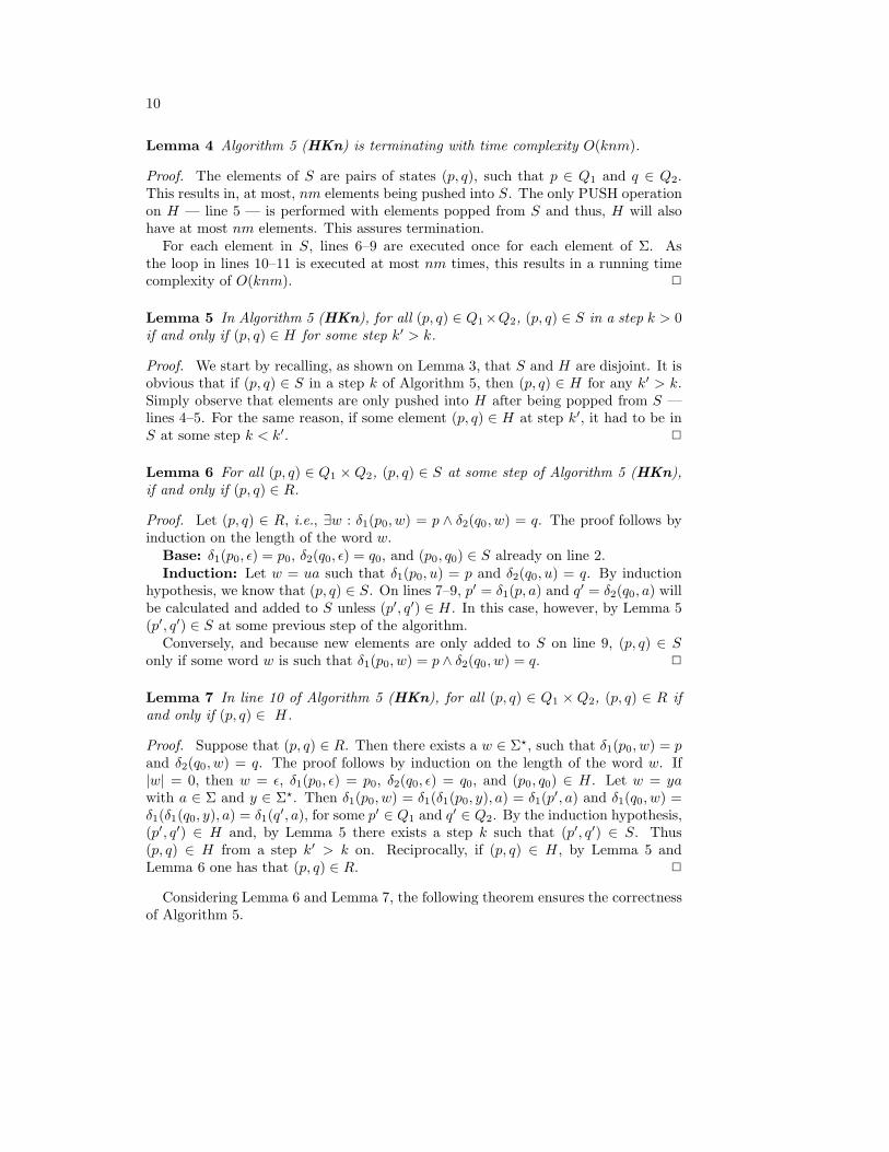
Lemma 4 Algorithm 5 (HKn) is terminating with time complexity O(knm).

Proof. The elements of S are pairs of states (p, q), such that p ∈ Q1 and q ∈ Q2.This results in, at most, nm elements being pushed into S. The only PUSH operationon H — line 5 — is performed with elements popped from S and thus, H will alsohave at most nm elements. This assures termination.

For each element in S, lines 6–9 are executed once for each element of Σ. Asthe loop in lines 10–11 is executed at most nm times, this results in a running timecomplexity of O(knm). 2

Lemma 5 In Algorithm 5 (HKn), for all (p, q) ∈ Q1×Q2, (p, q) ∈ S in a step k > 0if and only if (p, q) ∈ H for some step k′ > k.

Proof. We start by recalling, as shown on Lemma 3, that S and H are disjoint. It isobvious that if (p, q) ∈ S in a step k of Algorithm 5, then (p, q) ∈ H for any k′ > k.Simply observe that elements are only pushed into H after being popped from S —lines 4–5. For the same reason, if some element (p, q) ∈ H at step k′, it had to be inS at some step k < k′. 2

Lemma 6 For all (p, q) ∈ Q1 × Q2, (p, q) ∈ S at some step of Algorithm 5 (HKn),if and only if (p, q) ∈ R.

Proof. Let (p, q) ∈ R, i.e., ∃w : δ1(p0, w) = p ∧ δ2(q0, w) = q. The proof follows byinduction on the length of the word w.

Base: δ1(p0, ǫ) = p0, δ2(q0, ǫ) = q0, and (p0, q0) ∈ S already on line 2.Induction: Let w = ua such that δ1(p0, u) = p and δ2(q0, u) = q. By induction

hypothesis, we know that (p, q) ∈ S. On lines 7–9, p′ = δ1(p, a) and q′ = δ2(q0, a) willbe calculated and added to S unless (p′, q′) ∈ H . In this case, however, by Lemma 5(p′, q′) ∈ S at some previous step of the algorithm.

Conversely, and because new elements are only added to S on line 9, (p, q) ∈ Sonly if some word w is such that δ1(p0, w) = p ∧ δ2(q0, w) = q. 2

Lemma 7 In line 10 of Algorithm 5 (HKn), for all (p, q) ∈ Q1 × Q2, (p, q) ∈ R ifand only if (p, q) ∈ H.

Proof. Suppose that (p, q) ∈ R. Then there exists a w ∈ Σ⋆, such that δ1(p0, w) = pand δ2(q0, w) = q. The proof follows by induction on the length of the word w. If|w| = 0, then w = ǫ, δ1(p0, ǫ) = p0, δ2(q0, ǫ) = q0, and (p0, q0) ∈ H . Let w = yawith a ∈ Σ and y ∈ Σ⋆. Then δ1(p0, w) = δ1(δ1(p0, y), a) = δ1(p

′, a) and δ1(q0, w) =δ1(δ1(q0, y), a) = δ1(q

′, a), for some p′ ∈ Q1 and q′ ∈ Q2. By the induction hypothesis,(p′, q′) ∈ H and, by Lemma 5 there exists a step k such that (p′, q′) ∈ S. Thus(p, q) ∈ H from a step k′ > k on. Reciprocally, if (p, q) ∈ H , by Lemma 5 andLemma 6 one has that (p, q) ∈ R. 2

Considering Lemma 6 and Lemma 7, the following theorem ensures the correctnessof Algorithm 5.

11

Theorem 2 Let A and B be DFAs. A ∼ B if and only if for all (p, q) ∈ R, ε(p) =ε(q).

Proof. Suppose, by absurd, that A and B are not equivalent and that the conditionholds. Then, there exists w ∈ Σ⋆ such that ε(δ(p0, w)) 6= ε(δ(q0, w)). But in that casethere is a contradiction because (δ(p0, w), δ(q0, w)) ∈ R. On the other hand, if thereexists a (p, q) ∈ R such that ε(p) 6= ε(q), obviously A and B are not equivalent. 2

The relation R can be seen as a relation on Q1∪Q2 which is reflexive and symmetric.Its transitive closure R⋆ is an equivalence relation.

Lemma 8 ∀(p, q) ∈ R, ε(p) = ε(q) if and only if ∀(p, q) ∈ R⋆, ε(p) = ε(q).

Proof. Let (p, q), (q, r) ∈ R. Since R⋆ is the transitive closure of R, (p, r) ∈ R⋆ and ifε(p) = ε(q), then ε(p) = ε(r). On the other hand, as R ⊆ R⋆, if ε(p) = ε(q) ∀(p, q) ∈R⋆, the same will be true for every (p, q) ∈ R. 2

Corollary 1 A ∼ B if and only if ∀(p, q) ∈ R⋆, ε(p) = ε(q).

Algorithm HK computes R⋆ by starting with the finest partition in Q1 ∪ Q2 (theidentity). And if A ∼ B, R⋆ is a right-invariance.

Corollary 2 Algorithm 5 (HKn) and Algorithm 1 (HK) are equivalent.

4.3. Equivalence of the two methods

It is possible to use Algorithm 4 (AM) to obtain a DFA from each of the regularexpressions α and β in the following way. Let Dα = (Qα, Σ, δα, qα, Fα) and Dβ =(Qβ , Σ, δβ, qβ , Fβ) the equivalent DFAs to α and β, respectively. They are constructedin the following way:

• initialize Qα = α, Qβ = β;

• qα = α, qβ = β;

• for each instruction α′ = a−1(α), add the transition δα(α, a) = α′ and makeQα = Qα ∪ α′ (same for β and β′);

• whenever ε(α) = 1, make Fα = Fα ∪ α (same for β).

Qα and Qβ are the Brzozowski’s automata of the regular expressions α and β, respec-tively.

In order to prove the equivalence of Algorithm 1 (HK) and Algorithm 4 (AM), wewill first apply Theorem 1 to Algorithm 5 (HKn), transforming it into a refutationprocedure. This modified version is presented as Algorithm 6. We will then show thatthe regular expressions equivalence test AM actually embeds Hopcroft and Karp’smethod while constructing the equivalent DFAs.

12

1 def HK(A,B) t :2 S = (p0, q0)3 H = ∅4 while (p, q) = POP(S ) :5 i f ε(p) 6= ε(q) : return Fal s e6 PUSH(H, (p, q))7 for a ∈ Σ :8 p′ = δ1(p, a)9 q′ = δ2(q, a)

10 i f (p′, q′) /∈ H:11 PUSH(S , (p′, q′))12 return True

Algorithm 6 A naıve version of Hopcroft and Karp’s algorithm with refutation.

Lemma 9 Algorithm 4 (AM) embeds Algorithm 5 (HKn) while constructing theBrzozowski’s DFAs.

Proof. By Theorem 1, Algorithm 6 is equivalent to Algorithm 5, but including arefutation step. To verify that Algorithm 4 actually embeds Algorithm 6 while con-structing the Brzozowski’s DFAs, the following observations should be enough. Theinstructions

α′ = a−1(α); β′ = a−1(β)

from Algorithm 4 are trivially equivalent to

p′ = δ1(p, a); q′ = δ2(q, a)

in Algorithm 6, by the very definition of the method which constructs the equivalentDFAs.

The halting conditions are also the same. As p ∈ Fα if and only if ε(α) = ǫ,we know that ε(α′) 6= ε(β′) if and only if ε(p′) 6= ε(q′) when we consider the DFAsassociated to each of the regular expressions, such that p′ ∈ Qα, q′ ∈ Qβ . 2

Theorem 3 Algorithm 4 (AM) corresponds to Algorithm 1 (HK) applied to theBrzozowski’s automata of the two regular expressions.

Proof. By Corollary 2, Algorithm 5 and Algorithm 1 are equivalent. ApplyingLemma 9 we have that Algorithm 4 embeds Algorithm 5 while constructing the Br-zozowski’s DFAs. Thus, applying Algorithm 4 to two regular expressions α and β isequivalent to the application of Algorithm 1 to the Brzozowski’s automata of α andβ. 2

4.4. Improving Algorithm AM with Union-Find

Considering the Theorem 3 and the Corollary 2, we can improve the Algorithm 4(AM) for testing the equivalence of two r.e. α and β, by considering Algorithm 1applied to the Brzozowski’s automata correspondent to the two r.e. Instead of using

13

a stack (H) in order to keep an history of the pairs of regular expressions whichhave already been tested, we can build the correspondent equivalence relation R⋆ (asdefined for Lemma 8). Two main changes must be considered:

• One must ensure that the sets of derivatives of each regular expression aredisjoint. For that we consider their disjoint sum, where derivatives w.r.t. aword u are represented by tuples (u−1(α), 1) and (u−1(β), 2), respectively.

• In the UNION-FIND method, the FIND operation needs an equality test on theelements of the set. Testing the equality of two r.e.— even syntactic equality —is already a computationally expensive operation, and tuple comparison will beeven slower. On the other hand, integer comparison, can be considered to beO(1). As we know that each element of the set is unique, we may consider somehash function which assures that the probability of collision for these elements isextremely low. This allows us to safely use the hash values as the elements of theset, and thus, arguments to the FIND operation, instead of the r.e. themselves.This is also a natural procedure in the implementations of conversions from r.e.to automata.

We call equivUF to the resulting algorithm. The experimental results are pre-sented on Table 3, Section 5.

4.5. Worst-case complexity analysis

In this subsection we exhibit a family of regular expressions for which a non-deterministic version of the AM comparison method is exponential on the number ofletters |α|Σ of the regular expression α.

We proceed by showing that the NFA N of a regular expression α, obtained usingpartial derivatives [6] with the method described by Almeida et al. [5], is such that|N | ∈ O(|α|Σ) and the number of states of the smallest equivalent DFA is exponentialon |N |.

Partial derivatives are related to NFAs in the same natural way as derivativesare related to DFAs. Let α be a regular expression and α′ = a−1(α). The partialderivatives of α w.r.t. the letter a ∈ Σ, denoted by ∂a(α), can be seen as the set ofthe operands of the disjunction α′. The following recursive definition computes theset of partial derivatives of an arbitrary regular expression w.r.t a letter a.

∂a(∅) = ; ∂a(α + β) = ∂a(α) ∪ ∂a(β);

∂a(ǫ) = ; ∂a(αβ) = ∂a(α)β ∪ ε(α)∂a(β);

∂a(b) =

ǫ, if b = a;

, otherwise;∂a(α⋆) = ∂a(α)α⋆.

This definition can trivially be extended to words and clearly L(a−1(α)) =L(

∑∂a(α)). The set of all partial derivatives is finite [6] and denoted by PD(α).

Figure 1 presents a classical example of a bad behaved case (with n + 1 states) ofthe powerset construction, by Hopcroft et al. [13]. Although this example does notreach the 2n+1 states bound, the smallest equivalent DFA has exactly 2n states.

14

q0 q1 q2 qn−1 qn

a, b

a a, b a, b

Figure 1: NFA which has no equivalent DFA with less than 2n states.

Consider the regular expression family αℓ = (a+b)⋆(a(a+b)ℓ), where |αℓ|Σ = 3+2ℓ.It is easy to see that the NFA in Figure 1 is obtained directly from the application ofthe non-deterministic AM method to αℓ, with the corresponding partial derivativespresented on Figure 2.

αℓ (a + b)ℓ (a + b)ℓ−1 (a + b) ǫ

a, b

a a, b a, b

Figure 2: NFA obtained from the r.e. αℓ using the AM method.

The set of the partial derivatives PD(αℓ) = αℓ, (a+ b)ℓ, . . . , (a+ b), ǫ has ℓ+2 =n + 1 elements, which corresponds to the size of the obtained NFA. The equivalentminimal DFA has 2n = 2ℓ+1 states.

5. Experimental results

In this section we present some experimental results of the previously discussed al-gorithms applied to DFAs, NFAs, and regular expressions We also include the sameresults of the tests using Hopcroft’s (Hop) [11] and Brzozowski’s (Brz) [8] automataminimization algorithms. Due to space constraints, the full set of experimental resultscan be found in Appendix A.

The random DFAs were generated using publicly available tools5 [2]. The NFAsdataset was obtained with a set of tools described by Almeida et al. [4]. As theICDFAs datasets were obtained with a uniform random generator, the size of eachsample (10 000 elements) is sufficient to ensure a 95% confidence level within a 1%error margin. It is calculated with the formula n = ( z

2ǫ)2, where z is obtained from

the normal distribution table such that P (−z < Z < z)) = γ, ǫ is the error margin,and γ is the desired confidence level.

All the algorithms were implemented in the Python programming language. Thetests were executed in the same computer, an Intel R© Xeon R© 5140 at 2.33GHz with4GB of RAM.

Table 1 shows the results of experimental tests with 10000 pairs of complete ICD-FAs. We present the results for automata with n ∈ 5, 50 states over an alphabet ofk ∈ 2, 50 symbols. Clearly, the methods which do not rely in minimisation processesare a lot faster. Column Eff. shows the effective time spent by the algorithm itselfwhile column Total presents the total time spent, including overheads, such as making

5http://www.ncc.up.pt/FAdo/

15

n = 5 n = 50

k = 2 k = 50 k = 2 k = 50

Alg. Time (s) Iter. Time (s) Iter. Time (s) Iter. Time (s) Iter.

Eff. Total Avg. Eff. Total Avg. Eff. Total Avg. Eff. Total Avg.

Hop 5.3 7.3 - 85.2 91.0 - 566.8 572 - 17749.7 17787.5 -

Brz 25.5 28.0 - 1393.6 1398.9 - - - - - - -

HK 2.3 4.0 8.9 25.3 28.9 9.0 23.2 28.9 98.9 317.5 341.6 99.0

HKe 0.9 2.1 2.4 5.4 10.5 2.4 1.4 5.9 2.6 14.3 34.9 3.4

HKs 0.6 1.3 2.4 2.8 4.6 2.4 0.8 2.0 2.7 9.1 21.3 3.4

HKn 0.7 2.2 3.0 51.5 56.2 29.7 1.3 6.8 3.7 29.4 51.7 15.4

Table 1: Running times for tests with 10 000 uniformly generated ICDFAs.

a DFA complete, initializing auxiliary data structures, etc. All times are expressed inseconds, and the algorithms that were not finished within a 10 hours time span areaccordingly signaled. Brzozowski’s algorithm, Brz, is by far the slowest. Hopcroft’salgorithm, Hop, although faster, is still several orders of magnitude slower than anyof the algorithms of the previous sections. We also present the average number ofiterations (Iter.) used by each of the versions of algorithm HK, per pair of automata.Clearly, the refutation process is an advantage. HKn running times show that alinear set merging algorithm (such as UNION-FIND) is by far a better choice thana simple history (set) with pairs of states. HKs is a version of HKe which uses theautomata string representation proposed by Almeida et al. [2, 19]. The simplicity ofthe representation seemed to be quite suitable for this algorithm, and actually cutdown both running times to roughly half. This is an example of the impact that agood data structure may have on the overall performance of this algorithm.

n = 5 n = 50

k = 2 k = 20 k = 2 k = 20



Transition Density d = 0.1

Hop 10.3 12.5 - 1994.7 2003.2 - 660.1 672.9 - - - -

Brz 8.4 10.6 - 866.6 876.2 - 264.5 278.4 - - - -

HKe 0.8 2.9 2.2 8.4 19 4 24.4 37.8 10.2 - - -


Hop 17.9 19.8 - 2759.4 2767.5 - 538.7 572.6 - - - -

Brz 14.4 16 - 2189.3 2191.6 - 614.9 655.7 - - - -

HKe 2.6 4.3 4.9 36.3 47.3 10.3 6.8 48.9 2.5 294.6 702.3 11.5


Hop 12.5 14.3 - 376.9 385.5 - 1087.3 1134.2 - - - -

Brz 14 15.8 - 177 179.6 - 957.5 1014.3 - - - -

HKe 1.4 3.2 2.7 39 49.9 10.7 7.3 64.8 2.5 440.5 986.6 11.5

Table 2: Running times for tests with 10 000 random NFAs.

Table 2 shows the results of applying the same set of algorithms to NFAs. Thetesting conditions and notation are as before, adding only the transition density d asa new variable, which we define as the ratio of the number of transitions over the totalnumber of possible transitions (kn2). Although it is clear that HKe is faster, by atleast one order of magnitude, than any of the other algorithms, the peculiar behaviourof this algorithm with different transition densities is not easy to explain. Consideringthe simplest example of 5 states and 2 symbols, the dataset with a transition densityd = 0.5 took roughly twice as long as those with d ∈ 0.1, 0.8. On the other extreme,making n = 50 and k = 2, the hardest instance was d = 0.1, with the cases where

16

d ∈ 0.5, 0.8 present similar running times almost five times faster. In our largesttest, with n = 50 and k = 20, neither Hop nor Brz finished within the imposed timelimit. Again, d = 0.1 was the hardest instance for HKe, which also did not finishwithin the time limit, although the cases where d ∈ 0.5, 0.8 present similar runningtimes.

Size/Alg. Hop Brz AMo Equiv EquivP HKe EquivUF

k = 2 10 21.025 19.06 26.27 7.78 5.51 7.27 5.10

50 319.56 217.54 297.23 36.13 28.05 64.12 28.69

75 1043.13 600.14 434.89 35.79 23.46 139.12 60.09

100 7019.61 1729.05 970.36 60.76 48.29 183.55 124.00

k = 5 10 42.06 25.99 32.73 9.96 7.25 8.69 6.48

50 518.16 156.28 205.41 33.75 26.84 67.7 21.53

75 943.65 267.12 292.78 35.09 25.17 161.84 28.61

100 1974.01 386.72 567.39 54.79 45.41 196.13 37.02

k = 10 10 61.60 31.04 38.27 10.87 8.39 9.26 7.47

50 1138.28 198.97 184.93 34.93 28.95 72.95 22.60

75 2012.43 320.37 271.14 35.77 26.92 195.88 30.61

100 4689.38 460.84 424.67 52.97 44.58 194.01 39.23

Table 3: Running times (seconds) for tests with 10 000 random r.e.

Table 3 presents the running times of the application of HKe to regular expres-sions and their comparison with the algorithms presented by Almeida et al. [3], whereequiv and equivP are the functional variants of the original algorithm by Antimirovand Mosses (AMo). The NFAs were computed with Glushkov’s algorithm, as de-scribed by Yu [23]. equivUF is the UNION-FIND improved version of equivP.Although the results indicate that HKe is not as fast as the direct comparison meth-ods presented in the cited paper, it is clearly faster than any minimisation process.The improvements of equivUF over equivP are not significant (it is actually consid-erably slower for regular expressions of length 100 with 2 symbols). We suspect thatthis is related to some optimizations applied by the Python interpreter. We state thisbased on the fact that when both algorithms are executed using a profiler, equivUF

is almost twice faster than equivP on most tests.

We have no reason to believe that similar tests with different implementations ofthese algorithms would produce significantly different ordering of its running timesfrom the one here presented. However, it is important to keep in mind, that these areexperimental tests that greatly depend on the hardware, data structures, and severalimplementation details (some of which, such as compiler optimizations, we do notutterly control).

6. Conclusions

As minimality or equivalence for (finite) transition systems is in general intractable,right-invariant relations (bisimulations) have been extensively studied for nondeter-ministic variants of these systems. When considering deterministic systems, however,those relations provide non-trivial improvements. We presented several variants of amethod by Hopcroft and Karp for the comparison of DFAs without resorting to min-imisation and extended it to NFAs. This approach provides much more time-efficientmethods for checking the equivalence of automata and regular expressions. By placing

17

a refutation condition earlier in the algorithm we may achieve better running timesin the average case. This is sustained by the experimental results presented in thepaper. Using Brzozowski’s automata, we showed that a modified version of Antimirovand Mosses method translates directly to Hopcroft and Karp’s algorithm.

References

[1] A. V. Aho, J. E. Hopcroft, J. D. Ullman, The Design and Analysis ofComputer Algorithms. Addison-Wesley, 1974.

[2] M. Almeida, N. Moreira, R. Reis, Enumeration and Generation with a StringAutomata Representation. Theoret. Comput. Sci. 387 (2007) 2, 93–102.

[3] M. Almeida, N. Moreira, R. Reis, Antimirov and Mosses’s rewrite systemrevisited. In: O. Ibarra, B. Ravikumar (eds.), CIAA 2008: 13th InternationalConference on Implementation and Application of Automata. Number 5448 inLNCS, Springer, 2008, 46–56.

[4] M. Almeida, N. Moreira, R. Reis, On the performance of automata min-imization algorithms. In: A. Beckmann, C. Dimitracopoulos, B. Lowe

(eds.), CiE 2008: Abstracts and extended abst. of unpublished papers . 2008.

[5] M. Almeida, N. Moreira, R. Reis, Antimirov and Mosses’s rewrite systemrevisited. International Journal of Foundations of Computer Science 20 (2009)04, 669 – 684.

[6] V. M. Antimirov, Partial Derivatives of Regular Expressions and Finite Au-tomaton Constructions. Theoret. Comput. Sci. 155 (1996) 2, 291–319.

[7] V. M. Antimirov, P. D. Mosses, Rewriting Extended Regular Expressions.In: G. Rozenberg, A. Salomaa (eds.), Developments in Language Theory.World Scientific, 1994, 195 – 209.

[8] J. A. Brzozowski, Canonical Regular Expressions and Minimal State Graphsfor Definite Events. In: J. Fox (ed.), Proc. of the Sym. on Math. Theory ofAutomata. MRI Symposia Series 12, NY, 1963, 529–561.

[9] J. A. Brzozowski, Derivatives of Regular Expressions. JACM 11 (1964) 4,481–494.

[10] T. H. Cormen, C. E. Leiserson, R. L. Rivest, C. Stein, Introduction toAlgorithms . MIT, 2003.

[11] J. Hopcroft, An n log n algorithm for minimizing states in a finite automaton.In: Proc. Inter. Symp. on the Theory of Machines and Computations . AcademicPress, Haifa, Israel, 1971, 189–196.

[12] J. Hopcroft, R. M. Karp, A linear algorithm for testing equivalence of finiteautomata. Technical Report 71-114, University of California, 1971.

[13] J. Hopcroft, R. Motwani, J. D. Ullman, Introduction to Automata Theory,Languages and Computation. Addison Wesley, 2000.

18

[14] J. Hopcroft, J. D. Ullman, A linear list merging algorithm. Technical report,Princeton University, 1971.

[15] J. Hopcroft, J. D. Ullman, Set merging algorithms. SIAM J. Comput. 2

(1973) 4, 294–303.

[16] D. Kozen, On the Coalgebraic Theory of Kleene Algebra with Tests. Comput-ing and Information Science Technical Reports http://hdl.handle.net/1813/10173, Cornell University, 2008.

[17] D. C. Kozen, A completeness theorem for Kleene algebras and the algebra ofregular events. Infor. and Comput. 110 (1994) 2, 366–390.

[18] D. C. Kozen, Automata and Computability. Undergrad. Texts in ComputerScience, Springer, 1997.

[19] R. Reis, N. Moreira, M. Almeida, On the Representation of Finite Au-tomata. In: C. Mereghetti, B. Palano, G. Pighizzini, D.Wotschke (eds.),Proc. of DCFS’05 . Rap. Tec. DICO, Univ. di Studi Milano, IFIP, Como, Italy,2005, 269–276.

[20] J. Rutten, Behavioural differential equations: a coinductive calculus of streams,automata, and power series. Theoret. Comput. Sci. 208 (2003) 1–3, 1–53.

[21] A. Salomaa, Two Complete Axiom Systems for the Algebra of Regular Events.Journal of the Association for Computing Machinery 13 (1966) 1, 158–169.

[22] R. E. Tarjan, Efficiency of a Good But Not Linear Set Union Algorithm. JACM22 (1975) 2, 215 – 225.

[23] S. Yu, Regular languages. In: G. Rozenberg, A. Salomaa (eds.), Handbookof Formal Languages . 1, Springer, 1997.

19

A. Experimental results

n = 5

k = 2 k = 20 k = 50

Alg. Time (s) Iter. Time (s) Iter. Time (s) Iter.

Eff. Total Avg. Eff. Total Avg. Eff. Total Avg.

Hop 4.8 6.0 - 34.1 36.4 - 84.3 87.8 -

Brz 17.8 19.2 - 356.6 358.9 - 874.8 878.3 -

HK 2.2 3.8 8.9 11.6 13.6 9.0 24.2 28.5 9.0

HKe 0.8 2.2 2.4 2.4 4.4 2.4 4.9 8.1 2.4

HKs 0.5 1.2 2.4 1.4 2.5 2.4 3.0 4.8 2.4

HKn 0.7 1.9 3.0 7.5 9.7 11.3 42.4 46.0 25.7

n = 10

k = 2 k = 20 k = 50



Hop 16.3 17.9 - 161.7 165.1 - 425.0 431.8 -

Brz 276.5 278.2 - 30625.3 30614.6 - - - -

HK 4.9 6.7 18.9 22.5 24.0 19.0 51.8 56.2 19.0

HKe 0.9 2.7 2.5 2.8 6.3 2.6 5.7 11.5 2.6

HKs 0.5 1.3 2.5 2.0 3.6 2.6 3.6 6.7 2.6

HKn 0.6 2.4 3.2 9.0 12.1 12.2 47.9 53.2 27.0

n = 20

k = 2 k = 20 k = 50



Hop 61.6 64.3 - 742.6 748.1 - 1875.6 1886.1 -

Brz - - - - - - - - -

HK 9.3 12.1 38.9 44.9 48.9 39.0 118.4 126.7 39.0

HKe 1.2 3.7 2.7 3.7 8.9 3.0 7.0 17.1 2.9

HKs 0.6 1.6 2.7 2.5 5.6 3.0 5.2 11.1 2.9

HKn 0.9 3.3 3.6 9.4 14.6 12.3 55.2 65.3 31.3

n = 50

k = 2 k = 20 k = 50



Hop 510.8 516.1 - 6300.6 6312.4 - 16652.0 16676.3 -

Brz - - - - - - - - -

HK 23.9 29.2 98.9 124.5 135.0 99.0 298.5 318.3 99.0

HKe 1.3 7.0 2.7 5.3 18.5 3.4 10.6 36.0 3.4

HKs 0.7 2.2 2.7 4.3 10.7 3.4 8.8 23.5 3.4

HKn 1.1 6.3 3.7 14.0 26.7 17.4 28.1 53.2 15.4

Table 4: Running times for tests with 10 000 uniformly generated ICDFAs.

20

n = 5 n = 10

k = 2 k = 20 k = 2 k = 20




Hop 10.3 12.5 - 1994.7 2003.2 - 133.2 136.0 - - - -

Brz 8.4 10.6 - 866.6 876.2 - 117.4 120.3 - - - -

HKe 0.8 2.9 2.2 8.4 19 4 1.4 4.1 2.6 77.3 98.1 22.3


Hop 17.9 19.8 - 2759.4 2767.5 - 37.4 40.8 - 5617.9 5636.0 -

Brz 14.4 16 - 2189.3 2191.6 - 32.0 35.0 - 768.8 793.1 -

HKe 2.6 4.3 4.9 36.3 47.3 10.3 2.1 5.3 3.2 224.4 250.2 38.5


Hop 12.5 14.3 - 376.9 385.5 - 45.2 49.0 - 2348.0 2371.8 -

Brz 14 15.8 - 177 179.6 - 957.5 41.3 - 451.2 482.8 -

HKe 1.4 3.2 2.7 39 49.9 10.7 1.8 5.3 2.4 64.4 97.1 11.2

n = 50

k = 2 k = 20

Alg. Time (s) Iter. Time (s) Iter.


Hop 660.1 672.9 - - - -

Brz 264.5 278.4 - - - -

HKe 24.4 37.8 10.2 - - -


Hop 538.7 572.6 - - - -

Brz 614.9 655.7 - - - -

HKe 6.8 48.9 2.5 294.6 702.3 11.5


Hop 1087.3 1134.2 - - - -

Brz 957.5 1014.3 - - - -

HKe 7.3 64.8 2.5 440.5 986.6 11.5

Table 5: Running times for tests with 10 000 random NFAs.

Documents

Testing the Equivalence of Regular Languages 1