Testing for Weak Instruments in Linear IV Regressionmayoral.iae-csic.org/IV_2015/stock_yogo_2005.pdf84 Stock and Yogo bias-adjusted TSLS (BTSLS) (Nagar 1959; Rothenberg 1984). The

CHAPTER 5

Testing for Weak Instrumentsin Linear IV RegressionJames H. Stock and Motohiro Yogo

ABSTRACT

Weak instruments can produce biased IV estimators and hypothesis tests with large size distortions.But what, precisely, are weak instruments, and how does one detect them in practice? This paperproposes quantitative definitions of weak instruments based on the maximum IV estimator bias, orthe maximum Wald test size distortion, when there are multiple endogenous regressors. We tabulatecritical values that enable using the first-stage F-statistic (or, when there are multiple endogenousregressors, the Cragg–Donald [1993] statistic) to test whether the given instruments are weak.

1. INTRODUCTION

Standard treatments of instrumental variables (IV) regression stress that for in-struments to be valid they must be exogenous. It is also important, however, thatthe second condition for a valid instrument, instrument relevance, holds, for ifthe instruments are only marginally relevant, or “weak,” then first-order asymp-totics can be a poor guide to the actual sampling distributions of conventionalIV regression statistics.

At a formal level, the strength of the instruments matters because the naturalmeasure of this strength – the so-called concentration parameter – plays arole formally akin to the sample size in IV regression statistics. Rothenberg(1984) makes this point in his survey of approximations to the distributions ofestimators and test statistics. He considers the single equation IV regressionmodel

y = Yβ + u, (1.1)

where y and Y are T × 1 vectors of observations on the dependent variable andendogenous regressor, respectively, and u is a T × 1 vector of i.i.d. N (0, σ uu)errors. The reduced form equation for Y is

Y = ZΠ+ V, (1.2)

where Z is a T × K2 matrix of fixed, exogenous instrumental variables, Π isa K2 × 1 coefficient vector, and V is a T × 1 vector of i.i.d. N (0, σ V V ) errors,where corr(ut , Vt ) = ρ.

Weak Instruments in Linear IV Regression 81

The two-stage least-squares (TSLS) estimator of β is βTSLS = (Y′PZy)/(Y′PZY), where PZ = Z(Z′Z)−1Z′. Rothenberg (1984) expresses βTSLS as

µ(βTSLS − β) =(

σ uu

σ V V

)1/2ζ u + (SV u/µ)

1+ (2ζ V /µ)+ (SV V /µ2), (1.3)

where ζ u =Π′Z′u/(σ uuΠ′Z′ZΠ)1/2, ζ V =Π′Z′V/(σ V V Π′Z′ZΠ)1/2, SV u =V′PZu/(σ uuσ V V )1/2, SV V = V′PZV/σ V V , and µ is the square root of the con-centration parameter µ2 = Π′Z′ZΠ/σ V V .

Under the assumptions of fixed instruments and normal errors, ζ u and ζ V

are standard normal variables with correlation ρ, and SV u and SV V are elementsof a matrix with a central Wishart distribution. Because the distributions of ζ u ,ζ V , SV u , and SV V do not depend on the sample size, the sample size enters thedistribution of the TSLS estimator only through the concentration parameter.In fact, the form of (1.3) makes it clear that µ2 can be thought of as an effectivesample size, in the sense that µ formally plays the role usually associated with√

T . Rothenberg (1984) proceeds to discuss expansions of the distribution ofthe TSLS estimator in orders of µ, and he emphasizes that the quality of theseapproximations can be poor when µ2 is small. This has been underscored bythe dramatic numerical results of Nelson and Startz (1990a, 1990b) and Bound,Jaeger, and Baker (1995).

If µ2 is so small that inference based on some IV estimators and their con-ventional standard errors are potentially unreliable, then the instruments aresaid to be weak. But this raises two practical questions. First, precisely howsmall must µ2 be for instruments to be weak? Second, because Π, and thusµ2, is unknown, how is an applied researcher to know whether µ2 is in factsufficiently small and that his or her instruments are weak?

This paper provides answers to these two questions. First, we develop precise,quantitative definitions of weak instruments for the general case of n endoge-nous regressors. In our view, the matter of whether a group of instrumentalvariables is weak cannot be resolved in the abstract; rather, it depends on theinferential task to which the instruments are applied and how that inference isconducted. We therefore offer two alternative definitions of weak instruments.The first definition is that a group of instruments is weak if the bias of the IVestimator, relative to the bias of ordinary least squares (OLS), could exceed acertain threshold b, for example 10%. The second is that the instruments areweak if the conventional α-level Wald test based on IV statistics has an ac-tual size that could exceed a certain threshold r , for example r = 10% whenα = 5%. Each of these definitions yields a set of population parameters thatdefines weak instruments, that is, a “weak instrument set.” Because differentestimators (e.g., TSLS or LIML) have different properties when instruments areweak, the resulting weak instrument set depends on the estimator being used.For TSLS and other k-class estimators, we argue that these weak instrumentsets can be characterized in terms of the minimum eigenvalue of the matrixversion of µ2/K2.

82 Stock and Yogo

Second, given this quantitative definition of weak instrument sets, we showhow to test the null hypothesis that a given group of instruments is weak againstthe alternative that it is strong. Our test is based on the Cragg–Donald (1993)statistic; when there is a single endogenous regressor, this statistic is simply the“first-stage F-statistic,” the F-statistic for testing the hypothesis that the instru-ments do not enter the first stage regression of TSLS. The critical values for thetest statistic, however, are not Cragg and Donald’s (1993): our null hypothesis isthat the instruments are weak, even though the parameters might be identified,whereas Cragg and Donald (1993) test the null hypothesis of underidentifica-tion. We therefore provide tables of critical values that depend on the estimatorbeing used, whether the researcher is concerned about bias or size distortion,and the numbers of instruments and endogenous regressors. These critical val-ues are obtained using weak instrument asymptotic distributions (Staiger andStock 1997), which are more accurate than Edgeworth approximations whenthe concentration parameter is small.1

This paper is part of a growing literature on detecting weak instruments,surveyed in Stock, Wright, and Yogo (2002) and Hahn and Hausman (2003).Cragg and Donald (1993) proposed a test of underidentification, which (as dis-cussed earlier) is different from a test for weak instruments. Hall, Rudebusch,and Wilcox (1996), following the work by Bowden and Turkington (1984), sug-gested testing for underidentification using the minimum canonical correlationbetween the endogenous regressors and the instruments. Shea (1997) consid-ered multiple included regressors and suggested looking at a partial R2. NeitherHall et al. (1996) nor Shea (1997) provide a formal characterization of weakinstrument sets or a formal test for weak instruments, with controlled type Ierror, based on their respective statistics. For the case of a single endogenousregressor, Staiger and Stock (1997) suggested declaring instruments to be weakif the first-stage F-statistic is less than 10. Recently, Hahn and Hausman (2002)suggested comparing the forward and reverse TSLS estimators and conclud-ing that instruments are strong if the null hypothesis that these are the samecannot be rejected. Relative to this literature, the contribution of this paper istwofold. First, we provide a formal characterization of the weak instrument setfor a general number of endogenous regressors. Second, we provide a test ofwhether the given instruments fall in this set, that is, whether they are weak,where the size of the test is controlled asymptotically under the null of weakinstruments.

The rest of the paper is organized as follows. The IV regression model andthe proposed test statistic are presented in Section 2. The weak instrument setsare developed in Section 3. Section 4 presents the test for weak instruments andprovides critical values for tests based on TSLS bias and size, Fuller-k bias,and LIML size. Section 5 examines the power of the test, and conclusions arepresented in Section 6.

1 See Rothenberg (1984, p. 921) for a discussion of the quality of the Edgeworth approximationas a function of µ2 and K2.


2. THE IV REGRESSION MODEL, THE PROPOSEDTEST STATISTIC, AND WEAK INSTRUMENTASYMPTOTICS

2.1. The IV Regression Model

We consider the linear IV regression model (1.1) and (1.2), generalized to haven included endogenous regressors Y and K1 included exogenous regressors X:

y = Yβ + Xγ + u, (2.1)

Y = ZΠ+ XΦ+ V, (2.2)

where Y is now a T × n matrix of included endogenous variables, X is a T × K1

matrix of included exogenous variables (one column of which is 1’s if (2.1) in-cludes an intercept), Z is a T × K2 matrix of excluded exogenous variables tobe used as instruments, and the error matrix V is a T × n matrix. It is assumedthroughout that K2 ≥ n. Let Y = [y Y] and Z = [X Z] respectively denote thematrices of all the endogenous and exogenous variables. The conformable vec-tors β and γ and the matrices Π and Φ are unknown parameters. Throughoutthis paper, we exclusively consider inference about β.

Let Xt = (X1t · · · X K1t )′,Zt = (Z1t · · · Z K2t )′,Vt = (V1t · · · Vnt )′, and Zt =(X′

t Z′t )′ denote the vectors of the t th observations on these variables. Also let

Σ and Q denote the population second moment matrices,

E

[(ut

V t

) (u1 V′

t

)] = [σ uu ΣuV

ΣVu ΣVV

]= Σ and

E(Zt Z′t ) =

[QXX QXZ

QZX QZZ

]= Q. (2.3)

2.2. k-Class Estimators and Wald Statistics

Let the superscript “⊥” denote the residuals from the projection on X, so for ex-ample Y⊥ = MXY, where MX = I− X(X′X)−1X′. In this notation, the OLS es-timator of β is β = (Y⊥′Y⊥)−1(Y⊥′y). The k-class estimator of β is

β(k) = [Y⊥′(I− k MZ⊥ )Y⊥]−1[Y⊥′(I− k MZ⊥ )y⊥]. (2.4)

The Wald statistic, based on the k-class estimator, testing the null hypothesisthat β = β0, is

W (k) = [β(k)− β0]′[Y⊥′(I − kMZ⊥ )Y⊥][β(k)− β0]

nσ uu(k), (2.5)

where σ uu(k) = u⊥(k)′u⊥(k)/(T − K1 − n), where u⊥(k) = y⊥ − Y⊥β(k).This paper considers four specific k-class estimators: TSLS, the limited

information maximum likelihood estimator (LIML), the family of modi-fied LIML estimators proposed by Fuller (1977) (“Fuller-k estimators”), and

84 Stock and Yogo

bias-adjusted TSLS (BTSLS) (Nagar 1959; Rothenberg 1984). The values of kfor these estimators are (cf. Donald and Newey 2001):

TSLS: k = 1, (2.6)

LIML: k = kLIML is the smallest root of det (Y′MXY− kY′MZY) = 0,

(2.7)

Fuller-k: k = kLIML−c/(T−K1−K2),where c is a positive constant, (2.8)

BTSLS: k = T/(T − K2 + 2), (2.9)

where det(A) is the determinant of the matrix A. If the errors are symmetricallydistributed and the exogenous variables are fixed, LIML is median unbiasedto second order (Rothenberg 1983). In our numerical work, we examine theFuller-k estimator with c = 1, which is the best unbiased estimator to sec-ond order among estimators with k = 1+ a(kLIML − 1)− c/(T − K1 − K2)for some constants a and c (Rothenberg 1984). For further discussion, seeDonald and Newey (2001) and Stock et al. (2002, Section 6.1).

2.3. The Cragg–Donald Statistic

The proposed test for weak instruments is based on the eigenvalue of the matrixanalog of the F-statistic from the first-stage regression of TSLS,

GT = Σ−1/2′VV Y⊥′PZ⊥Y⊥Σ

−1/2VV

/K2, (2.10)

where ΣVV = (Y′MZY)/(T − K1 − K2).2 The test statistic is the minimumeigenvalue of GT :

gmin = mineval(GT ). (2.11)

This statistic was proposed by Cragg and Donald (1993) to test the nullhypothesis of underidentification, which occurs when the concentration matrixis singular. Instead, we are interested in the case that the concentration matrixis nonsingular but its eigenvalues are sufficiently small that the instrumentsare weak. To obtain the limiting null distribution of the Cragg–Donald statistic(2.11) under weak instruments, we rely on weak instrument asymptotics.

2.4. Weak Instrument Asymptotics: Assumptions and Notation

We start by summarizing the elements of weak instrument asymptotics fromStaiger and Stock (1997). The essential idea of weak instruments is that Z isonly weakly related to Y, given X. Specifically, weak instrument asymptoticsare developed by modeling Π as local to zero:

2 The definition of GT in (2.10) is GT in Staiger and Stock (1997, Equation (3.4)), divided by K2

to put it in F-statistic form.


Assumption LΠ. Π = ΠT = C/√

T , where C is a fixed K2 × n matrix.

Following Staiger and Stock (1997), we make the following assumption onthe moments:

Assumption M. The following limits hold jointly for fixed K2:

(a) (T−1u′u, T−1V′u, T−1V′V)p→ (σ uu,ΣVu,ΣVV);

(b) T−1Z′Zp→ Q;

(c) (T−1/2X′u, T−1/2Z′u, T−1/2X′V, T−1/2Z′V)d→ (ΨXu,ΨZu,ΨXV,

ΨZV), where Ψ ≡ [Ψ′Xu,Ψ

′Zu, vec(ΨXV)′, vec(ΨZV)′]′ is distributed

N (0,Σ⊗Q).

Assumption M can hold for time series or cross-sectional data. Part (c)assumes that the errors are homoskedastic.

Notation and Definitions. The following notation in effect transforms thevariables and parameters and simplifies the asymptotic expressions. Letρ = Σ−1/2′

VV ΣVuσ−1/2uu , θ = Σ−1

VVΣVu = σ1/2uu

−1/2VV ρ, λ = Ω1/2CΣ−1/2

VV , Λ =λ′λ/K2, and Ω = QZZ −QZXQ−1

XX QXZ. Note that ρ′ρ ≤ 1. Define the K2×1 and K2 × n random variables zu = Ω−1/2′(ΨZu −QZXQ−1

XXΨXu)σ−1/2uu and

zV = Ω−1/2′ (ΨZV – QZXQ−1XXΨXV)Σ−1/2

VV , so(zu

vec(zV)

)∼ N (0,Σ⊗ IK2 ), where Σ =

[1 ρ′

ρ In

]. (2.12)

Also let

ν1 = (λ+ zV)′(λ+ zV) and (2.13)

ν2 = (λ+ zV)′zu. (2.14)

2.5. Selected Weak Instrument Asymptotic Representations

We first summarize some results from Staiger and Stock (1997).

OLS Estimator. Under assumptions L and M, the probability limit of the OLS

estimator is βp→β + θ.

k-class Estimators. Suppose that T (k – 1)d→ κ . Then under assumptions L

and M,

β(k)− βd→ σ 1/2

uu −1/2VV (ν1 − κIn)−1(ν2 − κρ) and (2.15)

W (k)d→

(ν2 − κρ)′(ν1 − κIn)−1(ν2 − κρ)

n[1− 2ρ′(ν1 − κIn)−1(ν2 − κρ)+ (ν2 − κρ)′(ν1 − κIn)−2(ν2 − κρ)],

(2.16)

where (2.16) holds under the null hypothesis β = β0.

86 Stock and Yogo

For LIML and the Fuller-k estimators, κ is a random variable, while forTSLS and BTSLS κ is nonrandom. Let Ξ be the (n + 1) × (n + 1) matrix,Ξ = [zu(λ+ zV)]′[zu(λ+ zV)]. Then the limits in (2.15) and (2.16) hold with

TSLS: κ = 0, (2.17)

LIML: κ = κ∗, where κ∗ is the smallest root of det (Ξ− κΣ) = 0, (2.18)

Fuller-k: κ = κ∗ − c, where c is the constant in (2.8), and (2.19)

BTSLS: κ = K2 − 2. (2.20)

Note that the convergence in distribution of T (kLIML − 1)d→ κ∗ is joint with

the convergence in (2.15) and (2.16). For TSLS, the expressions in (2.15) and(2.16) simplify to

βTSLS − βd→ σ 1/2

uu −1/2VV ν−1

1 ν2 and (2.21)

W TSLS d→ ν ′2ν−11 ν2

n(1− 2ρ′ν−1

1 ν2 + ν ′2ν−21 ν2

) . (2.22)

Weak Instrument Asymptotic Representations: The Cragg–Donald Statistic.Under the weak instrument asymptotic assumptions, the matrix GT in (2.10)and the Cragg–Donald statistic (2.11) have the limiting distributions

GTd→ν1/K2 and (2.23)

gmind→mineval(ν1/K2). (2.24)

Inspection of (2.13) reveals that ν1 has a noncentral Wishart distribution withnoncentrality matrix λ′λ = K2Λ. This noncentrality matrix is the weak instru-ment limit of the concentration matrix

Σ−1/2VV Π′Z′ZΠΣ−1/2′

VVp→ K2Λ. (2.25)

Thus the weak instrument asymptotic distribution of the Cragg–Donaldstatistic gmin is that of the minimum eigenvalue of a noncentral Wishart, di-vided by K2, where the noncentrality parameter is K2Λ. To obtain criticalvalues for the weak instrument test based on gmin, we characterize the weakinstrument set in terms of the eigenvalues of Λ, the task taken up in the nextsection.

3. WEAK INSTRUMENT SETS

This section provides two general definitions of a weak instrument set, the firstbased on the bias of the estimator and the second based on size distortions of theassociated Wald statistic. These two definitions are then specialized to TSLS,


LIML, the Fuller-k estimator, and BTSLS, and the resulting weak instrumentsets are characterized in terms of the minimum eigenvalues of the concentrationmatrix.

3.1. First Characterization of a Weak Instrument Set: Bias

One consequence of weak instruments is that IV estimators are in general biased,so our first definition of a weak instrument set is in terms of its maximumbias.

When there is a single endogenous regressor, it is natural to discuss bias inthe units of β, but for n > 1, a bias measure must scale β so that the bias iscomparable across elements of β. A natural way to do this is to standardize theregressors Y⊥ so that they have unit standard deviation and are orthogonal or,equivalently, to rotate β by Σ1/2

Y⊥Y⊥ , where ΣY⊥Y⊥ = plim(Y⊥′Y⊥/T ). In thesestandardized units, the squared bias of an IV estimator, which we genericallydenote by βIV, is (EβIV − β)′ΣY⊥Y⊥ (EβIV – β). As our measure of bias, wetherefore consider the relative squared bias of the candidate IV estimator βIV,relative to the squared bias of the OLS estimator

B2T =

(EβIV − β)′ΣY⊥Y⊥ (EβIV − β)

(Eβ − β)′ΣY⊥Y⊥ (Eβ − β). (3.1)

If n = 1, then the scaling matrix in (3.1) drops out and the expression simpli-fies to BT = |EβIV − β|/|Eβ − β|. The measure (3.1) was proposed, but notpursued, in Staiger and Stock (1997).

The asymptotic relative bias, computed under weak instrument asymptotics,is denoted by B = lim T→∞BT . Under weak instrument asymptotics, E(β −β) → θ = σ

1/2uu Σ−1/2

VV ρ and ΣY⊥Y⊥ → ΣVV, so that the denominator in (3.1)has the limit (Eβ − β)′ΣY⊥Y⊥ (Eβ − β) → σ uuρ

′ρ. Thus for ρ′ρ > 0, thesquare of the asymptotic relative bias is

B2 = σ−1uu lim T→∞

(EβIV − β)′ΣY⊥Y⊥ (EβIV − β)

ρ′ρ. (3.2)

We deem instruments to be strong if they lead to reliable inferences forall possible degrees of simultaneity ρ; otherwise they are weak. Applied tothe relative bias measure, this leads us to consider the worst-case asymptoticrelative bias

Bmax = maxρ:0<ρ′ρ≤1

|B|. (3.3)

The first definition of a weak instrument set is based on this worst-casebias. We define the weak instrument set, based on relative bias, to consistof those instruments that have the potential of leading to asymptotic relativebias greater than some value b. In population, the strength of an instrument isdetermined by the parameters of the reduced form Equation (2.2). Accordingly,

88 Stock and Yogo

let Z = Π, ΣVV, Ω. The relative bias definition of weak instruments is

Wbias = Z: Bmax ≥ b. (3.4)

Relative Bias vs. Absolute Bias. Our motivation for normalizing the squaredbias measure by the bias of the OLS estimator is that it helps to separate thetwo problems of endogeneity (OLS bias) and weak instrument (IV bias). Forexample, in an application to estimating the returns to education, based on areading of the literature the researcher might believe that the maximum OLSbias is ten percentage points; if the relative bias measure in (3.1) is 0.1, then themaximum bias of the IV estimator is one percentage point. Thus formulatingthe bias measure in (3.1) as a relative bias measure allows the researcher toreturn to the natural units of the application using expert judgment about thepossible magnitude of the OLS bias.

This said, we will show that the maximal TSLS relative bias is also itsmaximal absolute bias in standardized units, so that for TSLS the maximalrelative and absolute bias can be treated interchangeably. We return to thispoint in Section 3.3.

3.2. Second Characterization of a Weak Instrument Set: Size

Our second definition of a weak instrument set is based on the maximal size ofthe Wald test of all the elements of β. In parallel to the approach for the biasmeasure, we consider an instrument strong from the perspective of the Wald testif the size of the test is close to its level for all possible configurations of the IVregression model. Let W IV denote the Wald test statistic based on the candidateIV estimator βIV. For the estimators considered here, under conventional first-order asymptotics, W IV has a chi-squared null distribution with n degrees offreedom, divided by n. The actual rejection rate RT under the null hypothesisis

RT = Prβ0

[W IV > χ2

n;α

/n], (3.5)

where χ2n;α is the α-level critical value of the chi-squared distribution with n

degrees of freedom and α is the nominal level of the test.In general, the rejection rate in (3.5) depends onρ. As in the definitions of the

bias-based weak instrument set, we consider the worst-case limiting rejectionrate

Rmax = maxρ:ρ′ρ≤1

R, where R = lim T→∞RT . (3.6)

The size-based weak instrument set Wsize consists of instruments that canlead to a size of at least r > α:

Wsize = Z: Rmax ≥ r. (3.7)

For example, if α = .05 then a researcher might consider it acceptable if theworst-case size is r = 0.10.


3.3. Weak Instrument Sets for TSLS

We now apply these general definitions of weak instrument sets to TSLS andargue that the sets can be characterized in terms of the minimum eigenvalueof Λ.

3.3.1. Weak Instrument Set Based on TSLS bias

Under weak instrument asymptotics,(BTSLS

T

)2 → ρ′h′hρρ′ρ

≡ (BTSLS)2

and (3.8)

(Bmax,TSLS)2 = maxρ:0<ρ′ρ≤1

ρ′h′hρρ′ρ

, (3.9)

where h = E[ν−11 (λ+ zV)′zV]. The asymptotic relative bias BTSLS depends on

ρ and λ, which are unknown, as well as on K2 and n.Because h depends on λ but not on ρ, by (3.8) we have Bmax,TSLS =

[maxeval(h′h)]1/2, where maxeval(A) denotes the maximum eigenvalue of thematrix A. By applying the singular value decomposition to λ, it is further possi-ble to show that the maximum eigenvalue of h′h depends only on K2, n, and theeigenvalues ofλ′λ/K2 = Λ. It follows that, for a given K2 and n, the maximumTSLS asymptotic bias is a function only of the eigenvalues of Λ.

When the number of instruments is large, it is possible to show further thatthe maximum TSLS asymptotic bias is a decreasing function of the minimumeigenvalue of Λ. Specifically, consider sequences of K2 and T such that K2 →∞ and T →∞ jointly, subject to K 4

2/T → 0, where Λ (which in generaldepends on K2) is held constant as K2 →∞.3 We write this joint limit as (K2,T →∞) and, following Stock and Yogo (2005), we refer to it as representing“many weak instruments.” It follows from (3.9) and Theorem 4.1(a) of Stockand Yogo (2003) that the many weak instrument limit of BTSLS

T is

lim(K2,T→∞)

(BTSLS

T

)2 = ρ′(Λ+ I)−2ρ

ρ′ρ. (3.10)

By solving the maximization problem (3.9), we obtain the many weak instru-ment limit, Bmax,TSLS = [1+mineval(Λ)]−1. It follows that, for many instru-ments, the set Wbias,TSLS can be characterized by the minimum eigenvalue ofΛ, and the TSLS weak instrument set Wbias,TSLS can be written as

Wbias,TSLS = Z: mineval(Λ) ≤ bias,TSLS(b; K2, n), (3.11)

where bias,TSLS(b; K2, n) is a decreasing function of the maximum allowablebias b.

Our formal justification for the simplification that Wbias,TSLS depends onlyon the smallest eigenvalue of Λ, rather than on all its eigenvalues, rests on

3 In Stock and Yogo (2005), the assumption that Λ is constant is generalized to consider sequencesof Λ, indexed by K2, that have a finite limit Λ∞ as K2 →∞.

90 Stock and Yogo

the many weak instrument asymptotic result (3.10). Numerical analysis forn = 2 suggests, however, that Bmax,TSLS is decreasing in each eigenvalue ofΛ for all values of K2. These numerical results suggest that the simplificationin (3.11), relying only on the minimum eigenvalue, is valid for all K2 underweak instrument asymptotics, even though we currently cannot provide a formalproof.4

3.3.2. Reinterpretation in Terms of Absolute Bias

Although Bmax was defined as maximal bias relative to OLS, for TSLS Bmax

is also the maximal absolute bias in standardized units. The numerator of(3.9) is evidently maximized when ρ′ρ = 1. Thus, for TSLS, (3.2) can be re-stated as (Bmax)2 = σ−1

uu maxρ:ρ′ρ=1 lim T→∞(EβTSLS − β)′Y⊥Y⊥ (EβTSLS −β). But (EβTSLS − β)′Y⊥Y⊥ (EβTSLS − β) is the squared bias of βTSLS, notrelative to the bias of the OLS estimator. For TSLS, then, the relative bias mea-sure can alternatively be reinterpreted as the maximal bias of the candidate IVestimator, in the standardized units of σ−1/2

uu Σ1/2Y⊥Y⊥ .

3.3.3. Weak Instrument Set Based on TSLS Size

For TSLS, it follows from (2.22) that the worst-case asymptotic size is

Rmax,TSLS = maxρ:ρ′ρ≤1

Pr

[ν ′2ν

−11 ν2

1− 2ρ′ν−11 ν2 + ν ′2ν

−21 ν2

> χ2n;α

].

(3.12)

Rmax,TSLS, and consequently Wsize,TSLS, depends only on the eigenvalues of Λas well as n and K2 (the reason is the same as for the similar assertion forBmax,TSLS).

When the number of instruments is large, the Wald statistic is maximizedwhenρ′ρ = 1 and is an increasing function of the eigenvalues ofΛ. Specifically,it is shown in Stock and Yogo (2005), Theorem 4.1(a), that the many weakinstrument limit of the TSLS Wald statistic, divided by K2, is

W TSLS/K2p→ ρ′(Λ+ In)−1ρ

n[1− 2ρ ′(Λ+ In)−1ρ+ ρ′(Λ+ In)−2ρ]. (3.13)

The right-hand side of (3.13) is maximized when ρ′ρ = 1, in which case thisexpression can be written asρ′(Λ+ In)−1ρ/n−1ρ′[In − (Λ+ In)−1]2ρ. In turn,the maximum of this ratio over ρ depends only on the eigenvalues of Λ and isdecreasing in those eigenvalues.

4 Because in general the maximal bias depends on all the eigenvalues, the maximal bias whenall the eigenvalues are equal to some value 0 might be greater than the maximal bias whenone eigenvalue is slightly less than 0 but the others are large. For this reason the set Wbias ispotentially conservative when K2 is small. This comment applies to size-based sets as well.


The many weak instrument limit of Rmax,TSLS is

Rmax,TSLS = maxρ:ρ′ρ≤1

lim(K2,T→∞)

Pr[W TSLS/K2 > χ2

n;α/nK2] = 1,

(3.14)

where the limit follows from (3.13) and from χ2n;α/(nK2) → 0. With many weak

instruments, the TSLS Wald statistic W TSLS is Op(K2), so that the boundaryof the weak instrument set, in terms of the eigenvalues of Λ, increases as afunction of K2 without bound.

For small values of K2, numerical analysis suggests that Rmax,TSLS is a non-increasing function of all the eigenvalues of Λ, which (if so) implies that theboundary of the weak instrument set can, for small K2, be characterized interms of this minimum eigenvalue. The argument leading to (3.11) thereforeapplies here and leads to the characterization

Wsize,TSLS = Z : mineval(Λ) ≤ size,TSLS(r ; K2, n, α), (3.15)

where size,TSLS(r ; K2, n, α) is decreasing in the maximal allowable size r .

3.4. Weak Instrument Sets for Other k-Class Estimators

The general definitions of weak instrument sets given in Sections 3.1 and 3.2can also be applied to other IV estimators. The weak instrument asymptoticdistribution for general k-class estimators is given in Section 2.2. What remainsto be shown is that the weak instrument sets, defined for specific estimators andtest statistics, can be characterized in terms of the minimum eigenvalue of Λ.As in the case of TSLS, the argument for the estimators considered here hastwo parts, for small K2 and for large K2.

For small K2, the argument applied for the TSLS bias can be used generallyfor k-class statistics to show that, given K2 and n, the k-class maximal relativebias and maximal size depend only on the eigenvalues of Λ. In general, thisdependence is complicated and we do not have theoretical results characterizingthis dependence. Numerical work for n = 1 and n = 2, however, indicates thatthe maximal bias and maximal size measures are decreasing in each of theeigenvalues of Λ in the relevant range of those eigenvalues.5 This in turn meansthat the boundary of the weak instrument set can be written in terms of theminimum eigenvalue of Λ, although this characterization could be conservative(see Footnote 4).

For large K2, we can provide theoretical results, based on many weak in-strument limits, showing that the boundary of the weak instrument set dependsonly on mineval(Λ). These results are summarized here.

5 It appears that there is some nonmonotonicity in the dependence on the eigenvalues for Fuller-kbias when the minimum eigenvalue is very small, but for such small eigenvalues the bias issufficiently large so that this nonmonotonicity does not affect the boundary eigenvalues.

92 Stock and Yogo

3.4.1. LIML and Fuller-k

As shown in Stock and Yogo (2003), Theorem 2(c), the LIML and Fuller-kestimators and their Wald statistics have the many weak instrument asymptoticdistributions√

K2(βLIML − β)d→ N

(0, σ uuΣ

−1/2VV Λ−1(Λ+ In − ρρ′)Λ−1Σ−1/2′

VV

), (3.16)

W LIML d→ x′(Λ+ In − ρρ′)1/2Λ−1(Λ+ In − ρρ′)1/2′x/n, where

x ∼ N (0, In), (3.17)

where these distributions are written for LIML but also apply to Fuller-k.An implication of (3.16) is that the LIML and Fuller-k estimators are consis-

tent under the sequence (K2, T ) →∞, a result shown by Chao and Swanson(2002) for LIML. Thus the many weak instrument maximal relative bias forthese estimators is zero.

An implication of (3.17) is that the Wald statistic is distributed as a weightedsum of n independent chi-squared random variables. When n = 1, it followsfrom (3.17) that the many weak instrument size has the simple form

Rmax,LIML = maxρ:ρ′ρ≤1

lim(K2,T→∞)

Pr[W LIML > χ2

1;α

]= Pr

[χ2

1 >Λ

Λ+ 1χ2

1;α

], (3.18)

that is, the maximal size is the tail probability that a chi-squared distribution withone degree of freedom exceeds [Λ/(Λ+ 1)]χ2

1;α . Evidently, this is decreasingin Λ and depends only on Λ (which, trivially, here is its minimum eigenvalue).

3.4.2. BTSLS

The many weak instrument asymptotic distributions of the BTSLS estimatorand Wald statistic are (Stock and Yogo 2003, Theorem 2(b))√

K2(βBTSLS−β)d→N

[0, σ uuΣ

−1/2VV Λ−1(Λ+ In+ρρ′)Λ−1Σ−1/2′

VV

],

(3.19)

W BTSLS d→ x′(Λ+ In + ρρ′)1/2Λ−1(Λ+ In + ρρ′)1/2′x/n, where

x ∼ N (0, In). (3.20)

It follows from (3.19) that the BTSLS estimator is consistent and that itsmaximal relative bias tends to zero under many weak instrument asymptotics.

For n = 1, the argument leading to (3.18) applies to BTSLS, except that thefactor is different: the many weak instrument limit of the maximal size is

Rmax,BTSLS = Pr

[χ2

1 >Λ

Λ+ 2χ2

1;α

], (3.21)

which is a decreasing function of Λ.


It is interesting to note that, according to (3.18) and (3.21), for a given valueof Λ the maximal size distortion of LIML and Fuller-k tests is less than that ofBTSLS when there are many weak instruments.

3.5. Numerical Results for TSLS, LIML, and Fuller-k

We have computed weak instrument sets based on maximum bias and size forseveral k-class statistics. Here, we focus on TSLS bias and size, Fuller-k (withc = 1 in (2.8)) bias, and LIML size. Additional results are reported in Stocket al. (2002). Because LIML does not have moments in finite samples, LIMLbias is not well defined so we do not analyze it here.

The TSLS maximal relative bias was computed by Monte Carlo simulationfor a grid of minimal eigenvalue of Λ from 0 to 30 for K2 = n + 2, . . . , 100,using 20,000 Monte Carlo draws. Computing the maximum TSLS bias entailscomputing h, defined following (3.8), by Monte Carlo simulation, given n, K2,and then computing the maximum bias [maxeval(h′h)]1/2. Computing the max-imum bias of Fuller-k and the maximum size distortions of TSLS and LIMLis more involved than computing the maximal TSLS bias because there is nosimple analytic solution to the maximum problem (3.6). Numerical analysisindicates that RTSLS is maximized when ρ′ρ = 1, and so the maximizationfor n = 2 was done by transforming to polar coordinates and performing agrid search over the half unit circle (half because of symmetry in (2.22)). ForFuller-k bias and LIML size, maximization was performed over this half circleand over 0 ≤ ρ′ρ ≤ 1. Because the bias and size measures appear to be de-creasing functions of all the eigenvalues, at least in the relevant range, we setΛ = In . The TSLS size calculations were performed using a grid of with 0≤ ≤ 75 (100,000 Monte Carlo draws); for Fuller-k bias, 0 ≤ ≤ 12 (50,000Monte Carlo draws); and for LIML size, 0 ≤ ≤ 10 (100,000 Monte Carlodraws).

The minimal eigenvalues of Λ that constitute the boundaries of Wbias,TSLS,Wsize,TSLS, Wbias,Fuller-k, and Wsize,LIML are plotted, respectively, in the top pan-els of Figures 5.1–5.4 for various cutoff values b and r . The figures show theboundary eigenvalues for n = 1; the corresponding plots of boundary eigenval-ues for n = 2 are qualitatively, and in many cases quantitatively, similar. Firstconsider the regions based on bias. The boundary of Wbias,TSLS is essentiallyflat in K2 for K2 sufficiently large. The boundary of the relative bias region forb = 0.1 (10% bias) asymptotes to approximately 8. In contrast, the boundary ofthe bias region for Fuller-k tends to zero as the number of instruments increases,which agrees with the consistency of the Fuller-k estimator under many weakinstrument asymptotics.

Turning to the regions based on size, the boundary of Wsize,TSLS dependsstrongly on K2; as suggested by (3.14), the boundary is approximately linear inK2 for K2 sufficiently large. The boundary eigenvalues are very large when thedegree of overidentification is large. For example, if one is willing to tolerate amaximal size of 15%, so the size distortion is 10% for the 5% level test, then

94 Stock and Yogo

Boundary of weak instrument set (n = 1)

0

4

8

12

16

20

24

0 10 20 30 40 50 60 70 80 90 100

K2

min

eval

Λ

Bias = 0.05

Bias = 0.3

Bias = 0.2

Bias = 0.1

Critical value at 5% significance (n = 1)

0

4

8

12

16

20

24

0 10 20 30 40 50 60 70 80 90 100

K2

gm

in

Bias = 0.05

Bias = 0.3

Bias = 0.2

Bias = 0.1

Figure 5.1. Weak instrument sets and critical values based on bias of TSLSrelative to OLS.

with 10 instruments the minimum eigenvalue boundary is approximately 20 forn = 1 (it is approximately 16 for n = 2). In contrast, the boundary of Wsize,LIML

decreases with K2 for both n = 1 and n = 2. Comparing these two plots showsthat tests based on LIML are far more robust to weak instruments than testsbased on TSLS.



0

50

100

150

200

250

0 10 20 30 40 50 60 70 80 90 100

K2

min

eval

Λ

Size = 0.1

Size = 0.25

Size = 0.2

Size = 0.15


0

50

100

150

200

250

0 10 20 30 40 50 60 70 80 90 100

K2

gm

in

Size = 0.1

Size = 0.25

Size = 0.2

Size = 0.15

Figure 5.2. Weak instrument sets and critical values based on size of TSLSWald test.

4. TEST FOR WEAK INSTRUMENTS

This section provides critical values for the weak instrument test based onthe Cragg–Donald (1993) statistic gmin. These critical values are based on theboundaries of the weak instrument sets obtained in Section 3 and on a boundon the asymptotic distribution of gmin.

96 Stock and Yogo


0

5

10

15

20

25

0 10 20 30 40 50 60 70 80 90 100K2

min

eval

Λ

Bias = 0.05

Bias = 0.3

Bias = 0.2Bias = 0.1


0

5

10

15

20

25

0 10 20 30 40 50 60 70 80 90 100K2

gm

in

Bias = 0.05

Bias = 0.3

Bias = 0.2

Bias = 0.1

Figure 5.3. Weak instrument sets and critical values based on bias of Fuller-krelative to OLS.

4.1. A Bound on the Asymptotic Distribution of gmin

Recall that the Cragg–Donald statistic gmin is the minimum eigenvalue ofGT , where GT is given by (2.10). As stated in (2.23), under weak in-strument asymptotics, K2GT is asymptotically distributed as a noncentralWishart with dimension n, degrees of freedom K2, identity covariance matrix,



0

3

6

9

12

15

18

0 10 20 30 40 50 60 70 80 90 100K2

min

eval

Λ

Size = 0.1Size = 0.25

Size = 0.2Size = 0.15


0

3

6

9

12

15

18

0 10 20 30 40 50 60 70 80 90 100K

2

gm

in

Size = 0.1

Size = 0.25

Size = 0.2Size = 0.15

Figure 5.4. Weak instrument sets and critical values based on size of LIMLWald test.

and noncentrality matrix K2Λ; that is,

GTd→ν1/K2 ∼ Wn(K2, In, K2Λ)/K2. (4.1)

The joint pdf for the n eigenvalues of a noncentral Wishart has an infiniteseries expansion in terms of zonal polynomials (Muirhead 1978). This joint

98 Stock and Yogo

pdf depends on all the eigenvalues of Λ, as well as n and K2. In principle thepdf for the minimum eigenvalue can be determined from this joint pdf for allthe eigenvalues. It appears that this pdf (the “exact asymptotic” pdf of gmin)depends on all the eigenvalues of Λ.

This exact asymptotic distribution of gmin is not very useful for applicationsboth because of the computational difficulties it poses and because of its de-pendence on all the eigenvalues of Λ. This latter consideration is especiallyimportant because in practice these eigenvalues are unknown nuisance param-eters, and so critical values that depend on multiple eigenvalues would producean infeasible test.

We circumvent these two problems by proposing conservative critical valuesbased on the following bounding distribution.

Proposition 4.1. Pr[mineval(Wn(k, In,A)) ≥ x] ≤ Pr[χ2k(mineval(A)) ≥ x],

where χ2k(a) denotes a noncentral chi-squared random variable with noncen-

trality parameter a.

Proof. Letα be the eigenvector of A corresponding to its minimum eigenvalue.Then α′Wα is distributed χ2

k(mineval(A)) (Muirhead 1982, Theorem 10.3.6).But α′Wα ≥ mineval(W), and the result follows.

Applying (4.1), the continuous mapping theorem, and Proposition 4.1, wehave

Pr[gmin ≥ x] → Pr[mineval(ν1/K2) ≥ x]

≤ Pr

[χ2

K2(mineval(K2Λ))

K2≥ x

]. (4.2)

Note that this inequality holds as an equality in the special case n = 1.Conservative critical values for the test based on gmin are obtained as follows.

First, select the desired minimal eigenvalue of Λ. Next, obtain the desiredpercentile, say the 95% point, of the noncentral chi-squared distribution withnoncentrality parameter equal to K2 times this selected minimum eigenvalue,and divide this percentile by K2.6

6 The critical values based on Proposition 4.1 can be quite conservative when all the eigenvalues ofΛ are small. For example, the boundary of the TSLS bias-based weak instrument set with b = 0.1,n = 2, and K2 = 4 is mineval(Λ) = 3.08, and the critical value for a 5% test with b = 0.1 basedon Proposition 1 is 7.56. If the second eigenvalue in fact equals the first, the correct criticalvalue should be 4.63, and the rejection probability under the null is only 0.1%. (Of course, it isinfeasible to use this critical value because the second eigenvalue of Λ is unknown.) If the secondeigenvalue is 10, then the rejection rate is approximately 2%. On the other hand, if the secondeigenvalue is large, the Proposition 1 bound is tighter. For example, for values of K2 from 4 to34 and n = 2, if the second eigenvalue exceeds 20 the rejection probability under the null rangesfrom 3.3% to 4.1% for the nominal 5% weak instrument test based on TSLS bias with b = 0.1.


4.2. The Weak Instruments Test

The bound (4.2) yields the following testing procedure to detect weak instru-ments. To be concrete, this is stated for a test based on the TSLS bias measurewith significance level 100δ%. The null hypothesis is that the instruments areweak, and the alternative is that they are not:

H0: Z ∈Wbias,TSLS vs. H1: Z /∈Wbias,TSLS. (4.3)

The test procedure is

Reject H0 if gmin ≥ dbias,TSLS(b; K2, n, δ), (4.4)

where dbias,TSLS(b; K2, n, δ) = K−12 χ2

K2,1−δ(K2bias,TSLS(b; K2, n)), whereχ2

K2,1−δ(m) is the 100(1− δ)% percentile of the noncentral chi-squareddistribution with K2 degrees of freedom and noncentrality parameter m, andthe function bias,TSLS is the weak instrument boundary minimum eigenvalueof Λ in (3.11).

The results of Section 3 and the bound resulting from Proposition 1 implythat, asymptotically, the test (4.4) has the desired asymptotic level:

lim T→∞Pr[gmin ≥ dbias,TSLS(b; K2, n, δ) | Z ∈Wbias,TSLS] ≤ δ.

(4.5)

The procedure for testing whether the instruments are weak from the per-spective of the size of the TSLS (or LIML) is the same, except that the criticalvalue in (4.4) is obtained using the size-based boundary eigenvalue function,size,TSLS(r ; K2, n, α) (or, for LIML, size,LIML(r ; K2, n, α)).

4.3. Critical Values

Given a minimum eigenvalue , conservative critical values for the test arepercentiles of the scaled noncentral chi-squared distribution χ2

K2,1−δ (K2)/K2.The minimum eigenvalue is obtained from the boundary eigenvalue functionsin Section 3.5.

Critical values are tabulated in Tables 5.1–5.4 for the weak instrument testsbased on TSLS bias,TSLS size, Fuller-k bias, and LIML size, respectively,for one and two included endogenous variables (and three for TSLS bias)and up to 30 instruments. These critical values are plotted in the panel be-low the corresponding boundaries of the weak instrument sets in Figures 5.1–5.4. The critical value plots are qualitatively similar to the correspondingboundary eigenvalue plots, except of course that the critical values exceed theboundary eigenvalues to take into account the sampling distribution of the teststatistic.

These critical value plots provide a basis for comparing the robustness toweak instruments of various procedures: the lower the critical value curve, the

Tabl

e5.

1.C

riti

calv

alue

sfo

rth

ew

eak

inst

rum

entt

estb

ased

onT

SLS

bias

(Sig

nific

ance

leve

lis

5%)

n=

1,b=

n=

2,b=

n=

3,b=

K2

0.05

0.10

0.20

0.30

0.05

0.10

0.20

0.30

0.05

0.10

0.20

0.30

313

.91

9.08

6.46

5.39

416

.85

10.2

76.

715.

3411

.04

7.56

5.57

4.73

518

.37

10.8

36.

775.

2513

.97

8.78

5.91

4.79

9.53

6.61

4.99

4.30

619

.28

11.1

26.

765.

1515

.72

9.48

6.08

4.78

12.2

07.

775.

354.

407

19.8

611

.29

6.73

5.07

16.8

89.

926.

164.

7613

.95

8.50

5.56

4.44

820

.25

11.3

96.

694.

9917

.70

10.2

26.

204.

7315

.18

9.01

5.69

4.46

920

.53

11.4

66.

654.

9218

.30

10.4

36.

224.

6916

.10

9.37

5.78

4.46

1020

.74

11.4

96.

614.

8618

.76

10.5

86.

234.

6616

.80

9.64

5.83

4.45

1120

.90

11.5

16.

564.

8019

.12

10.6

96.

234.

6217

.35

9.85

5.87

4.44

1221

.01

11.5

26.

534.

7519

.40

10.7

86.

224.

5917

.80

10.0

15.

904.

4213

21.1

011

.52

6.49

4.71

19.6

410

.84

6.21

4.56

18.1

710

.14

5.92

4.41

1421

.18

11.5

26.

454.

6719

.83

10.8

96.

204.

5318

.47

10.2

55.

934.

3915

21.2

311

.51

6.42

4.63

19.9

810

.93

6.19

4.50

18.7

310

.33

5.94

4.37

1621

.28

11.5

06.

394.

5920

.12

10.9

66.

174.

4818

.94

10.4

15.

944.

3617

21.3

111

.49

6.36

4.56

20.2

310

.99

6.16

4.45

19.1

310

.47

5.94

4.34

1821

.34

11.4

86.

334.

5320

.33

11.0

06.

144.

4319

.29

10.5

25.

944.

3219

21.3

611

.46

6.31

4.51

20.4

111

.02

6.13

4.41

19.4

410

.56

5.94

4.31

2021

.38

11.4

56.

284.

4820

.48

11.0

36.

114.

3919

.56

10.6

05.

934.

2921

21.3

911

.44

6.26

4.46

20.5

411

.04

6.10

4.37

19.6

710

.63

5.93

4.28

2221

.40

11.4

26.

244.

4320

.60

11.0

56.

084.

3519

.77

10.6

55.

924.

2723

21.4

111

.41

6.22

4.41

20.6

511

.05

6.07

4.33

19.8

610

.68

5.92

4.25

2421

.41

11.4

06.

204.

3920

.69

11.0

56.

064.

3219

.94

10.7

05.

914.

2425

21.4

211

.38

6.18

4.37

20.7

311

.06

6.05

4.30

20.0

110

.71

5.90

4.23

2621

.42

11.3

76.

164.

3520

.76

11.0

66.

034.

2920

.07

10.7

35.

904.

2127

21.4

211

.36

6.14

4.34

20.7

911

.06

6.02

4.27

20.1

310

.74

5.89

4.20

2821

.42

11.3

46.

134.

3220

.82

11.0

56.

014.

2620

.18

10.7

55.

884.

1929

21.4

211

.33

6.11

4.31

20.8

411

.05

6.00

4.24

20.2

310

.76

5.88

4.18

3021

.42

11.3

26.

094.

2920

.86

11.0

55.

994.

2320

.27

10.7

75.

874.

17

Not

es.T

hete

stre

ject

sif

g min

exce

eds

the

criti

calv

alue

.The

criti

calv

alue

isa

func

tion

ofth

enu

mbe

rof

incl

uded

endo

geno

usre

gres

sors

(n),

the

num

ber

ofin

stru

men

talv

aria

bles

(K2),

and

the

desi

red

max

imal

bias

ofth

eIV

estim

ator

rela

tive

toO

LS

(b).


Table 5.2. Critical values for the weak instrument test based on TSLS size(Significance level is 5%)

n = 1, r = n = 2, r =K2 0.10 0.15 0.20 0.25 0.10 0.15 0.20 0.25

1 16.38 8.96 6.66 5.532 19.93 11.59 8.75 7.25 7.03 4.58 3.95 3.633 22.30 12.83 9.54 7.80 13.43 8.18 6.40 5.454 24.58 13.96 10.26 8.31 16.87 9.93 7.54 6.285 26.87 15.09 10.98 8.84 19.45 11.22 8.38 6.896 29.18 16.23 11.72 9.38 21.68 12.33 9.10 7.427 31.50 17.38 12.48 9.93 23.72 13.34 9.77 7.918 33.84 18.54 13.24 10.50 25.64 14.31 10.41 8.399 36.19 19.71 14.01 11.07 27.51 15.24 11.03 8.85

10 38.54 20.88 14.78 11.65 29.32 16.16 11.65 9.3111 40.90 22.06 15.56 12.23 31.11 17.06 12.25 9.7712 43.27 23.24 16.35 12.82 32.88 17.95 12.86 10.2213 45.64 24.42 17.14 13.41 34.62 18.84 13.45 10.6814 48.01 25.61 17.93 14.00 36.36 19.72 14.05 11.1315 50.39 26.80 18.72 14.60 38.08 20.60 14.65 11.5816 52.77 27.99 19.51 15.19 39.80 21.48 15.24 12.0317 55.15 29.19 20.31 15.79 41.51 22.35 15.83 12.4918 57.53 30.38 21.10 16.39 43.22 23.22 16.42 12.9419 59.92 31.58 21.90 16.99 44.92 24.09 17.02 13.3920 62.30 32.77 22.70 17.60 46.62 24.96 17.61 13.8421 64.69 33.97 23.50 18.20 48.31 25.82 18.20 14.2922 67.07 35.17 24.30 18.80 50.01 26.69 18.79 14.7423 69.46 36.37 25.10 19.41 51.70 27.56 19.38 15.1924 71.85 37.57 25.90 20.01 53.39 28.42 19.97 15.6425 74.24 38.77 26.71 20.61 55.07 29.29 20.56 16.1026 76.62 39.97 27.51 21.22 56.76 30.15 21.15 16.5527 79.01 41.17 28.31 21.83 58.45 31.02 21.74 17.0028 81.40 42.37 29.12 22.43 60.13 31.88 22.33 17.4529 83.79 43.57 29.92 23.04 61.82 32.74 22.92 17.9030 86.17 44.78 30.72 23.65 63.51 33.61 23.51 18.35

Notes. The test rejects if gmin exceeds the critical value. The critical value is a function ofthe number of included endogenous regressors (n), the number of instrumental variables(K2), and the desired maximal size (r ) of a 5% Wald test of β = β0.

more robust is the procedure. For discussion and comparisons of TSLS, BTSLS,Fuller-k, JIVE, and LIML, see Stock et al. (2002, Section 6).

4.3.1. Comparison to the Staiger–Stock Rule of Thumb

Staiger and Stock (1997) suggested the rule of thumb that, in the n = 1 case,instruments be deemed weak if the first-stage F is less than 10. They motivated

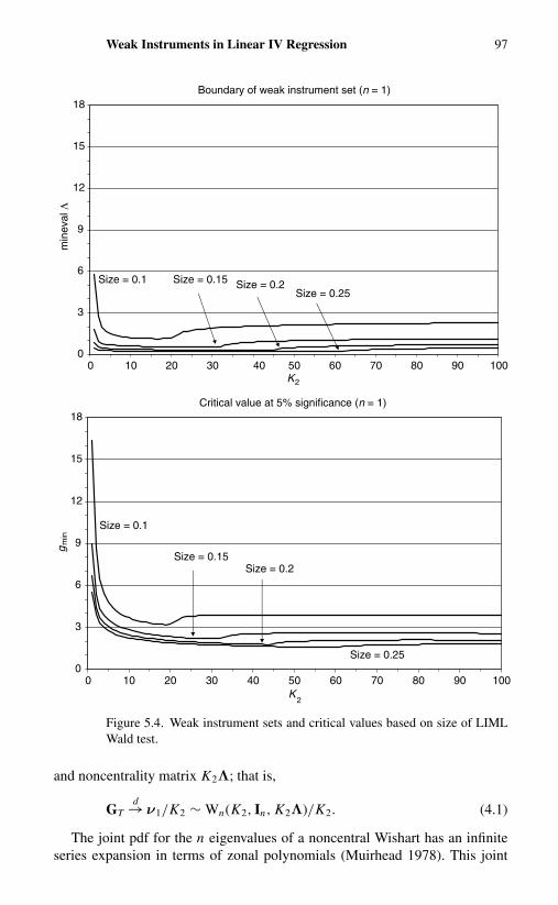
102 Stock and Yogo

Table 5.3. Critical values for the weak instrument test based on Fuller-k bias(Significance level is 5%)

n = 1, b = n = 1, b =K2 0.05 0.10 0.20 0.30 0.05 0.10 0.20 0.30

1 24.09 19.36 15.64 12.712 13.46 10.89 9.00 7.49 15.50 12.55 9.72 8.033 9.61 7.90 6.61 5.60 10.83 8.96 7.18 6.154 7.63 6.37 5.38 4.63 8.53 7.15 5.85 5.105 6.42 5.44 4.62 4.03 7.16 6.07 5.04 4.446 5.61 4.81 4.11 3.63 6.24 5.34 4.48 3.987 5.02 4.35 3.75 3.33 5.59 4.82 4.08 3.658 4.58 4.01 3.47 3.11 5.10 4.43 3.77 3.399 4.23 3.74 3.25 2.93 4.71 4.12 3.53 3.19

10 3.96 3.52 3.07 2.79 4.41 3.87 3.33 3.0211 3.73 3.34 2.92 2.67 4.15 3.67 3.17 2.8812 3.54 3.19 2.80 2.57 3.94 3.49 3.04 2.7713 3.38 3.06 2.70 2.48 3.76 3.35 2.92 2.6714 3.24 2.95 2.61 2.41 3.60 3.22 2.82 2.5815 3.12 2.85 2.53 2.34 3.47 3.11 2.73 2.5116 3.01 2.76 2.46 2.28 3.35 3.01 2.65 2.4417 2.92 2.69 2.39 2.23 3.24 2.92 2.58 2.3818 2.84 2.62 2.34 2.18 3.15 2.84 2.52 2.3319 2.76 2.56 2.29 2.14 3.06 2.77 2.46 2.2820 2.69 2.50 2.24 2.10 2.98 2.71 2.41 2.2321 2.63 2.45 2.20 2.07 2.91 2.65 2.36 2.1922 2.58 2.40 2.16 2.04 2.85 2.60 2.32 2.1623 2.52 2.36 2.13 2.01 2.79 2.55 2.28 2.1224 2.48 2.32 2.10 1.98 2.73 2.50 2.24 2.0925 2.43 2.28 2.06 1.95 2.68 2.46 2.21 2.0626 2.39 2.24 2.04 1.93 2.63 2.42 2.18 2.0327 2.36 2.21 2.01 1.90 2.59 2.38 2.15 2.0128 2.32 2.18 1.99 1.88 2.55 2.35 2.12 1.9829 2.29 2.15 1.96 1.86 2.51 2.31 2.09 1.9630 2.26 2.12 1.94 1.84 2.47 2.28 2.07 1.94

Notes. The test rejects if gmin exceeds the critical value. The critical value is a func-tion of the number of included endogenous regressors (n), the number of instru-mental variables (K2), and the desired maximal bias of the IV estimator relative toOLS (b).

this suggestion based on the relative bias of TSLS. Because the 5% criticalvalue for the relative bias weak instrument test with b = 0.1 is approximately11 for all values of K2, the Staiger–Stock rule of thumb is approximately a 5%test that the worst-case relative bias is approximately 10% or less. This providesa formal, and not unreasonable, testing interpretation of the Staiger–Stock ruleof thumb.


Table 5.4. Critical values for the weak instrument test based on LIML size(Significance level is 5%)

n = 1, r = n = 1, r =K2 0.10 0.15 0.20 0.25 0.10 0.15 0.20 0.25

1 16.38 8.96 6.66 5.532 8.68 5.33 4.42 3.92 7.03 4.58 3.95 3.633 6.46 4.36 3.69 3.32 5.44 3.81 3.32 3.094 5.44 3.87 3.30 2.98 4.72 3.39 2.99 2.795 4.84 3.56 3.05 2.77 4.32 3.13 2.78 2.606 4.45 3.34 2.87 2.61 4.06 2.95 2.63 2.467 4.18 3.18 2.73 2.49 3.90 2.83 2.52 2.358 3.97 3.04 2.63 2.39 3.78 2.73 2.43 2.279 3.81 2.93 2.54 2.32 3.70 2.66 2.36 2.20

10 3.68 2.84 2.46 2.25 3.64 2.60 2.30 2.1411 3.58 2.76 2.40 2.19 3.60 2.55 2.25 2.0912 3.50 2.69 2.34 2.14 3.58 2.52 2.21 2.0513 3.42 2.63 2.29 2.10 3.56 2.48 2.17 2.0214 3.36 2.57 2.25 2.06 3.55 2.46 2.14 1.9915 3.31 2.52 2.21 2.03 3.54 2.44 2.11 1.9616 3.27 2.48 2.18 2.00 3.55 2.42 2.09 1.9317 3.24 2.44 2.14 1.97 3.55 2.41 2.07 1.9118 3.20 2.41 2.11 1.94 3.56 2.40 2.05 1.8919 3.18 2.37 2.09 1.92 3.57 2.39 2.03 1.8720 3.21 2.34 2.06 1.90 3.58 2.38 2.02 1.8621 3.39 2.32 2.04 1.88 3.59 2.38 2.01 1.8422 3.57 2.29 2.02 1.86 3.60 2.37 1.99 1.8323 3.68 2.27 2.00 1.84 3.62 2.37 1.98 1.8124 3.75 2.25 1.98 1.83 3.64 2.37 1.98 1.8025 3.79 2.24 1.96 1.81 3.65 2.37 1.97 1.7926 3.82 2.22 1.95 1.80 3.67 2.38 1.96 1.7827 3.85 2.21 1.93 1.78 3.74 2.38 1.96 1.7728 3.86 2.20 1.92 1.77 3.87 2.38 1.95 1.7729 3.87 2.19 1.90 1.76 4.02 2.39 1.95 1.7630 3.88 2.18 1.89 1.75 4.12 2.39 1.95 1.75

Notes. The test rejects if gmin exceeds the critical value. The critical value is a function ofthe number of included endogenous regressors (n), the number of instrumental variables(K2), and the desired maximal size (r ) of a 5% Wald test of β = β0.

The rule of thumb fares less well from the perspective of size distortion.When the number of instruments is one or two, the Staiger–Stock rule of thumbcorresponds to a 5% level test that the maximum size is no more than 15%(so that the maximum TSLS size distortion is no more than 10%). However,when the number of instruments is moderate or large, the critical value is muchlarger and the rule of thumb does not provide substantial assurance that the sizedistortion is controlled.

104 Stock and Yogo

5. ASYMPTOTIC PROPERTIES OF THE TESTAS A DECISION RULE

This section examines the asymptotic rejection rate of the weak instrument testas a function of the smallest eigenvalue of Λ. When this eigenvalue exceedsthe boundary minimum eigenvalue for the weak instrument set, the asymptoticrejection rate is the asymptotic power function.

The exact asymptotic distribution of gmin depends on all the eigenvalues ofΛ.It is bounded above by (4.2). On the basis of numerical analysis, we conjecturethat this distribution is bounded below by the distribution of the minimumeigenvalue of a random matrix with the noncentral Wishart distribution Wn(K2,In , mineval(K2Λ)In)/K2. These two bounding distributions are used to boundthe distribution of gmin as a function of mineval(Λ).

The bounds on the asymptotic rejection rate of the test (4.4) (based onTSLS maximum relative bias) are plotted in Figure 5.5 for b = 0.1 and n = 2.The value of the horizontal axis (the minimum eigenvalue) at which the upperrejection rate curve equals 5% is bias(.1; K2, 2). Evidently, as the minimumeigenvalue increases, so does the rejection rate. The rejection curve becomessteeper as K2 increases. The bounding distributions give a fairly tight range forthe actual power function, which depends on all the eigenvalues of Λ.

The analogous curves for the test based on Fuller-k bias,TSLS size, orLIML size are centered differently because the tests have different critical val-ues but otherwise are qualitatively similar to those in Figure 5.5 and thus areomitted.

Interpretation as a Decision Rule

It is useful to think of the weak instrument test as a decision rule: if gmin isless than the critical value, conclude that the instruments are weak, otherwiseconclude that they are strong.

Under this interpretation, the asymptotic rejection rates in Figure 5.5 boundthe asymptotic probability of deciding that the instruments are strong. Evidently,for values of mineval(Λ) much below the weak instrument region boundary,the probability of correctly concluding that the instruments are weak is effec-tively equal to 1. Thus, if in fact the researcher is confronted by instrumentsthat are quite weak, this will be detected by the weak instruments test withprobability essentially equal to 1. Similarly, if the researcher has instrumentswith a minimum eigenvalue of Λ substantially above the threshold for the weakinstruments set, then the probability of correctly concluding that they are strongalso is essentially equal to 1.

The range of ambiguity of the decision procedure is given by the valuesof the minimum eigenvalue for which the asymptotic rejection rates effectivelyfall between 0 and 1. When K2 is small this range can be 10 or more, butfor K2 large this range of potential ambiguity of the decision rule is quitenarrow.


K2 = 4

0.0

0.2

0.4

0.6

0.8

1.0

0 2 4 6 8 10 12 14 16 18 20mineval Λ

Pow

er

K2 = 34

0.0

0.2

0.4

0.6

0.8

1.0

0 2 4 6 8 10 12 14 16 18 20mineval Λ

Pow

er

Figure 5.5. Power function for TSLS bias test (Relative bias = 0.1, n = 2).

6. CONCLUSIONS

The procedure proposed here is simple: compare the minimum eigenvalue ofGT , the first-stage F-statistic matrix, to a critical value. The critical value isdetermined by the IV estimator the researcher is using, the number of instru-ments K2, the number of included endogenous regressors n, and how muchbias or size distortion the researcher is willing to tolerate. The test statistic is

106 Stock and Yogo

the same whether one focuses on the bias of TSLS or Fuller-k or on the size ofTSLS or LIML; all that differs is the critical value.

Viewed as a test, the procedure has good power, especially when the numberof instruments is large. Viewed as a decision rule, the procedure effectivelydiscriminates between weak and strong instruments, and the region of ambiguitydecreases as the number of instruments increases.

Our findings support the view that LIML is far superior to TSLS whenthe researcher has weak instruments, at least from the perspective of coveragerates. Actual LIML coverage rates are close to their nominal rates even forquite small values of the concentration parameter, especially for moderatelymany instruments. Similarly, the Fuller-k estimator is more robust to weakinstruments than TSLS when viewed from the perspective of bias. Additionalcomparisons are made in Stock et al. (2002).

When there is a single included endogenous variable, this procedure providesa refinement and improvement to the Staiger–Stock (1997) rule of thumb thatinstruments be deemed “weak” if the first-stage F is less than 10. The differencebetween that rule of thumb and the procedure of this paper is that, instead ofcomparing the first-stage F to 10, it should be compared to the appropriateentry in Table 5.1 (TSLS bias), Table 5.2 (TSLS size), Table 5.3 (Fuller-k bias),or Table 5.4 (LIML size). Those critical values indicate that their rule of thumbcan be interpreted as a test, with approximately a 5% significance level, of thehypothesis that the maximum relative bias is at least 10%. The Staiger–Stockrule of thumb is too conservative if LIML or Fuller-k are used unless the numberof instruments is very small, but it is insufficiently conservative to ensure thatthe TSLS Wald test has good size.

This paper has two loose ends. First, the characterization of the set of weakinstruments is based on the premise that the maximum relative bias and themaximum size distortion are nonincreasing in each eigenvalue of Λ, for valuesof those eigenvalues in the relevant range. This was justified formally usingthe many weak instrument asymptotics of Stock and Yogo (2003); althoughnumerical analysis suggests it is true for all K2, this remains to be proven.Second, the lower bound of the power function in Section 5 is based on theassumption that the cdf of the minimum eigenvalue of a noncentral Wishartrandom variable is nondecreasing in each of the eigenvalues of its noncen-trality matrix. This too appears to be true on the basis of numerical analysis,but we do not have a proof, nor does this result seem to be available in theliterature.

Beyond this, several avenues of research remain open. First, the tests pro-posed here are conservative when n > 1 because they use critical values com-puted using the noncentral chi-squared bound in Proposition 4.1. Althoughthe tests appear to have good power despite this, tightening the Proposi-tion 4.1 bound (or constructing tests based on all the eigenvalues) could pro-duce more powerful tests. Second, we have considered inference based onTSLS, Fuller-k, and LIML, but there are other estimators to explore as well.Third, the analysis here is predicated upon homoskedasticity, and it remains to


extend these tests to GMM estimation of the linear IV regression model underheteroskedasticity.

ACKNOWLEDGMENTS

We thank Alastair Hall, Jerry Hausman, Takesi Hayakawa, George Judge,Whitney Newey, and Jonathan Wright for helpful comments and/or suggestions.This research was supported by NSF grants SBR-9730489 and SBR-0214131.

References

Bound, J., D. A. Jaeger, and R. M. Baker (1995), “Problems with Instrumental Vari-ables Estimation when the Correlation Between the Instruments and the EndogenousExplanatory Variable is Weak,” Journal of the American Statistical Association, 90,443–50.

Bowden, R., and D. Turkington (1984), Instrumental Variables. Cambridge: CambridgeUniversity Press.

Chao, J. C., and N. R. Swanson (2002), “Consistent Estimation with a Large Numberof Weak Instruments,” unpublished manuscript, University of Maryland.

Cragg, J. G., and S. G. Donald (1993), “Testing Identifiability and Specification inInstrumental Variable Models,” Econometric Theory, 9, 222–40.

Donald, S. G., and W. K. Newey (2001), “Choosing the Number of Instruments,” Econo-metrica, 69, 1161–91.

Fuller, W. A. (1977): “Some Properties of a Modification of the Limited InformationEstimator,” Econometrica, 45, 939–53.

Hall, A., G. D. Rudebusch, and D. Wilcox (1996), “Judging Instrument Relevance inInstrumental Variables Estimation,” International Economic Review, 37, 283–98.

Hahn, J., and J. Hausman (2002), “A New Specification Test for the Validity of Instru-mental Variables,” Econometrica, 70, 163–89.

Hahn, J., and J. Hausman (2003), “Weak Instruments: Diagnosis and Cures in Em-pirical Econometrics,” American Economic Review, Papers and Proceedings, 93,118–25.

Muirhead, R. J. (1978), “Latent Roots and Matrix Variates: A Review of Some Asymp-totic Results,” Annals of Statistics, 6, 5–33.

Muirhead, R. J. (1982), Aspects of Multivariate Statistical Theory. New York: Wiley.Nagar, A. L. (1959), “The Bias and Moment Matrix of the General k-Class Estimators

of the Parameters in Simultaneous Equations,” Econometrica, 27, 575–95.Nelson, C. R., and R. Startz (1990a), “Some Further Results on the Exact Small Sample

Properties of the Instrumental Variables Estimator,” Econometrica, 58, 967–76.Nelson, C. R., and R. Startz (1990b), “The Distribution of the Instrumental Variables

Estimator and Its t-Ratio when the Instrument is a Poor One,” Journal of Business,63, 5125–40.

Rothenberg, T. J. (1983), “Asymptotic Properties of Some Estimators in Structural Mod-els,” in (ed. by S. Karlin, T. Amemiya, and L. Goodman), Studies in Econometrics,Time Series, and Multivariate Statistics. Orlando: Academic Press.

Rothenberg, T. J. (1984), “Approximating the Distributions of Econometric Estimatorsand Test Statistics,” Chapter 15 in Handbook of Econometrics, Vol. II (ed. by Z.Griliches and M. D. Intriligator), Amsterdam: North Holland, 881–935.

108 Stock and Yogo

Shea, J. (1997), “Instrument Relevance in Multivariate Linear Models: A Simple Mea-sure,” Review of Economics and Statistics, 79, 348–52.

Staiger, D., and J. H. Stock (1997): “Instrumental Variables Regression with WeakInstruments,” Econometrica, 65, 557–86.

Stock, J. H., J. H. Wright, and M. Yogo (2002), “A Survey of Weak Instruments andWeak Identification in Generalized Method of Moments,” Journal of Business andEconomic Statistics, 20, 518–29.

Stock, J. H., and M. Yogo (2005), “Asymptotic Distributions of Instrumental VariablesStatistics with Many Weak Instruments,” Chapter 6 in this volume.

Documents

Testing for Weak Instruments in Linear IV Regressionmayoral.iae-csic.org/IV_2015/stock_yogo_2005.pdf84 Stock and Yogo bias-adjusted TSLS (BTSLS) (Nagar 1959; Rothenberg 1984). The