Testing for Unit Roots in Panel Databhhall/papers... · Panel Data: An Exploration Using Real and Simulated Data Bronwyn H. HALL UC Berkeley, Oxford University, and NBER Jacques MAIRESSE

Testing for Unit Roots in Panel Data:

An Exploration Using Real and Simulated Data

Bronwyn H. HALLUC Berkeley, Oxford University, and NBER

Jacques MAIRESSEINSEE-CREST, EHESS, and NBER

3/12/02 NSF Symposium - Berkeley 2

Introduction

! Our Research Program:! Develop simple models that describe the time series behavior of

key variables for a panel of firms:• Sales, employment, profits, investment, R&D• U.S., France, Japan

! Substantive interest: use of these variables for further modeling (productivity, investment, etc.) requires an understanding of their univariate behavior

! Technical interest: explore the use of a number of estimators and tests that have been proposed in the literature, using real data.

! This paper: a comparison of unit root tests for fixed T, large N panels, using DGPs that mimic the behavior of our real data.


Outline

! Basic features of our data! Motivation – issues in estimating a

simple dynamic panel model! Overview of unit root tests for short

panels! Simulation results! Results for real data


Dataset CharacteristicsScientific Sector, 1978-1989

Country France United States JapanData sources Enquete annuelle sur les Standard and Poor’s Needs data;

moyens consacres a la Compustat data – Data from recherche et au dev. annual industrial and OTC JDB (R&Ddans les entreprises;enq. OTC, based on 10-K data fromannuelle des entreprises filings to SEC Toyo Keizai

survey)# firms 953 863 424# observations 5,842 6,417 5,088After cleaning 5,139 5,721 4,260No jumps 5,108 5,312 4,215Balanced 1978-89

(# obs.) 1,872 2,448 2,652(# firms) 156 204 221

Positive Cash Flow(# firms) 104 174 200

The scientific sector consists of firms in Chemicals, Pharmaceuticals, Electrical Machinery, Computing Equipment, Electronics, and Scientific Instruments.


Variables! Sales (millions $)! Employment (1000s)! Investment (P&E, millions $)! R&D (millions $)! Cash flow (millions $)All variables in logarithms, overall year

means removed (so price level changes common to all firms are removed – Levin and Lin 1993).


Representative data - salesLo

g of

def

late

d sa

les

Selected U.S. Manufacturing FirmsYear

1975 1980 1985 1990

-5

0

5


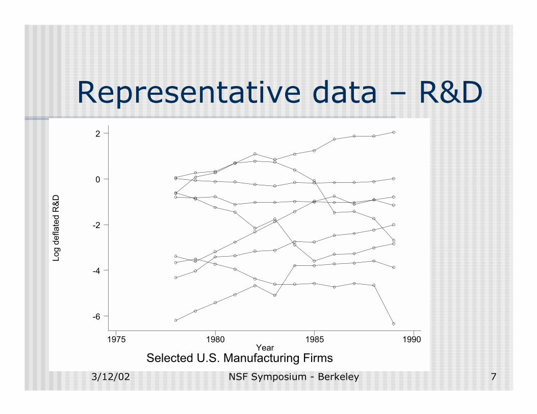
Representative data – R&DLo

g de

flate

d R

&D

Selected U.S. Manufacturing FirmsYear

1975 1980 1985 1990

-6

-4

-2

0

2


Autocorrelation Function for Real VariablesUnited States

0.0

0.2

0.4

0.6

0.8

1.0

0 1 2 3 4 5 6 7 8 9 10 11

Lag

Aut

ocor

rela

tion

Sales R&D Employment Investment Cash Flow


Autocorrelation Function for Differenced Logs of Real VariablesUnited States

-1.0

-0.8

-0.6

-0.4

-0.2

0.0

0.2

0.4

0.6

0.8

1.0

0 1 2 3 4 5 6 7 8 9 10

Lag

Aut

ocor

rela

tion

Sales R&D Employment Investment Cash Flow


Variance of Log Growth Rates

-7.0 -6.5 -6.0 -5.5 -5.0 -4.5 -4.0 -3.5 -3.0 -2.5 -2.0 -1.5 -1.0

0.05

0.10

0.15

0.20

0.25

0.30

0.35 Estimated Log(Sigsq(i)) Distribution for Differenced Log Sales - U. S.

0.000 0.025 0.050 0.075 0.100 0.125 0.150 0.175 0.200 0.225 0.250 0.275 0.300

5

10

15

20

25

Estimated Sigsq(i) for Differenced Log Sales - U.S.

Num

ber of obs.

Var(log growth rate)

σ2(i) log σ2(i)


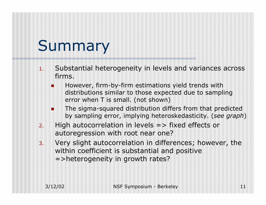
Summary1. Substantial heterogeneity in levels and variances across

firms.! However, firm-by-firm estimations yield trends with

distributions similar to those expected due to sampling error when T is small. (not shown)

! The sigma-squared distribution differs from that predicted by sampling error, implying heteroskedasticity. (see graph)

2. High autocorrelation in levels => fixed effects or autoregression with root near one?

3. Very slight autocorrelation in differences; however, the within coefficient is substantial and positive =>heterogeneity in growth rates?


A Simple Model

1 if :)(

)())(1(:)(

)1(

or 0 ),0(~

Years,...,1 ;Firms ,...,1

interest. of variable the of logarithm

1,

1,

1,1

2

1

=++∆==>

++∆++−==>

++−+−=

≠≠===

+=++=

=

−

−

−−

−

ρεδεδρδαρ

ερρδδρα

σε

ερδα

ittitit

ittittiit

ittittiit

jsitiit

ititit

ittiit

it

yyRW

yyFE

yy

ijs,t]εE[ε

TtNi

uu

uy

y


Estimation with a Firm Effect

Drop δt (means removed) and difference out αi:

OLS is inconsistent; use IV or GMM-IV for estimation with yi,t-2,…,yi1 as instruments.

Advantages: robust to heteroskedasticity and non-normality; consistent for β’s; allows for some types of transitory measurement error in y.

Disadvantages: biased in finite samples; imprecise when instruments are weakly correlated with independent variables.

ittiit yy ερ ∆+∆=∆ −1,


Three Data Generating Processes

OLS is consistent; IV with lagged instruments not identified.

OLS is inconsistent; IV or GMM with lag 2+ inst. is consistent

OLS is inconsistent; IV or GMM with lag 2+ inst. is consistent

itit

ittiit

y

yy

εδεδρ

+=∆

++=⇒≡ −

or

1.1 1,

itit

itiit

y

ty

εδεδαρ

∆+=∆++=⇒=

or

0.2

ittiit

ittiit

yy

tyy

εδρεδραρ

∆++∆=∆

+++=⇒<

−

−

1,

1,

or

effects no ,1.3


Results of SimulationN=200 T=12 No. of draws=1000

Estimated coefficient for dy on dy(-1)Instruments are y(-2)-y(-4)

-0.010 (.333)

0.440(.228)**

GMM2

-0.006(.041)

-0.047(.168)

GMM CUE

0.868 (.089)

-0.059 (.025)**

rho=0.9(no effects)

-0.028 (0.042)

0.000(.046)

-0.500(0.019)**

rho=0.0(FE)

-0.040(.175)

0.279 (.690)

-0.001(.026)

rho=1.0(RW)

GMM1IVOLSTruth

** Different from truth at 5% level of significance.


Conclusion from Simulations! As with ordinary times series, it is essential to

test first for a unit root (even though asymptotics in the panel data case are for N and not T).

! Failure to do so may lead to the use of estimators that are very biased and misleading in finite samples even though they are consistent. ! If unit root => assume no fixed effect and then OLS

level estimators appropriate.! If no unit root => fixed effect (usually) and IV.! Near unit root => OLS bias can be large.


Unit Root Tests ConsideredNote that these tests are generally valid for large N

and fixed T.! IPS: Im, Pesaran, and Shim (1995) –

alternative is ρi <1 for some i. Based on an average of augmented Dickey-Fuller tests conducted firm by firm, with or without trend.Normal disturbances assumed.

! HT: Harris-Tzavalis (JE 1999) – alternative is ρ<1. Based on the LSDV estimator, corrected for bias and normalized by the theoretical std. error under the null. Homoskedastic normal disturbances assumed.


Unit Root Tests (continued)! SUR: OLS with no fixed effects and an equation for each year

(suggested by Bond et al 2000) – consistent under the null of a unit root. Has good power. Allows for heteroskedasticity and correlation over time easily.

! CMLE:! Kruiniger (1998, 1999) – CMLE is consistent for stationary model

and for ρ=1 (fixed T). Use an LR test based on this fact. Homoskedastic normal disturbances assumed, but not necessary.

! Lancaster and Lindenhovius (1996); Lancaster (1999) – similar to Kruiniger. Bayesian estimation with flat prior on effects and 1/σ for the variance yields estimates that are consistent when ρ=1 (fixed T). σ is shrunk slightly toward zero.

! CMLE-HS: suggested in Kruiniger (1998) – heteroskedasticity of the form σi

2 σt2 can be estimated consistently.


Conditional ML Estimation (HS)Model: Or

Stacking the model:

With

ittiiit yy εραρ ++−= −1,)1(

),0(~ 21, iitittiit

itiit

Nuu

uy

σεερ

α

+=

+=

−

iii uy += ια

−==

−−

−

−

−

1...............

...

...1

...1

1]'[

21

32

2

1

2

22

TT

T

T

T

iiii VuuE

ρρ

ρρρρρρρ

ρσσ ρ


Conditional ML Estimation (HS)

Differenced:

The log likelihood function:

−−

−

==

1...000...............0...1000...1100...011

where DDuDy ii

Φ==ΣΣ⇒ 22 with ),0(~ iii D' DVNDy σσ ρ

{ }

∑

∑

=

−

=

Φ−Φ−

−−−−=

N

i i

ii

i

N

ii

DyDyN

TTNL

12

1

2

1

2

)'(21

log2

)log(2

)1()2log(

2)1(

),(log

σ

σπσρ



The σi2 can be concentrated out using

which yields

for estimation.

( ))'(1

1 12iii DyDytr

T−Φ

−=σ

)(log2

))(log(2

)1(

)12log(2

)1()(log

2

1

ρρσ

πρ

Φ−−−

+−−=

∑=

NT

TNL

i

N

i



! Kruiniger (1999) proves consistency of the CMLE-HS estimator for ρ!(-1,1].

! However, the concentrated or profile likelihood version is problematic:! Nuisance parameters (σi

2) increase with N – standard error estimates biased downward; not efficient (see B-N & Cox, ex. 4.3).

! Non-orthogonal parameters (ρ, σt2, and σi

2)

! Possible alternatives:! Modified profile likelihood - Barndorff-Nielsen and Cox

(1994), but not clear how to do this.! Integrated likelihood (Woutersen 2000).


Results of Simulations! IPS

! zero augmenting lags to be consistent with other tests. ! we found size was too large if the data were allowed to

choose the number of augmenting lags.! size slightly too large! power weak against large rho alternatives.

! HT! size correct if homoskedastic; ! power weak against large rho alternatives, with or without

FE.! SUR

! size correct; slightly too large if heteroskedastic! power weak against large rho alternatives, with or without

FE.


Results of Simulations

! CMLE! size correct if homoskedastic! power weak against large rho alternatives, with or

without FE

! CMLE-HS! size wrong! power slightly weak against large rho alternatives, with

or without FE! requires sandwich var-cov estimator; appears to have

downward-biased standard errors, so rejects too often.


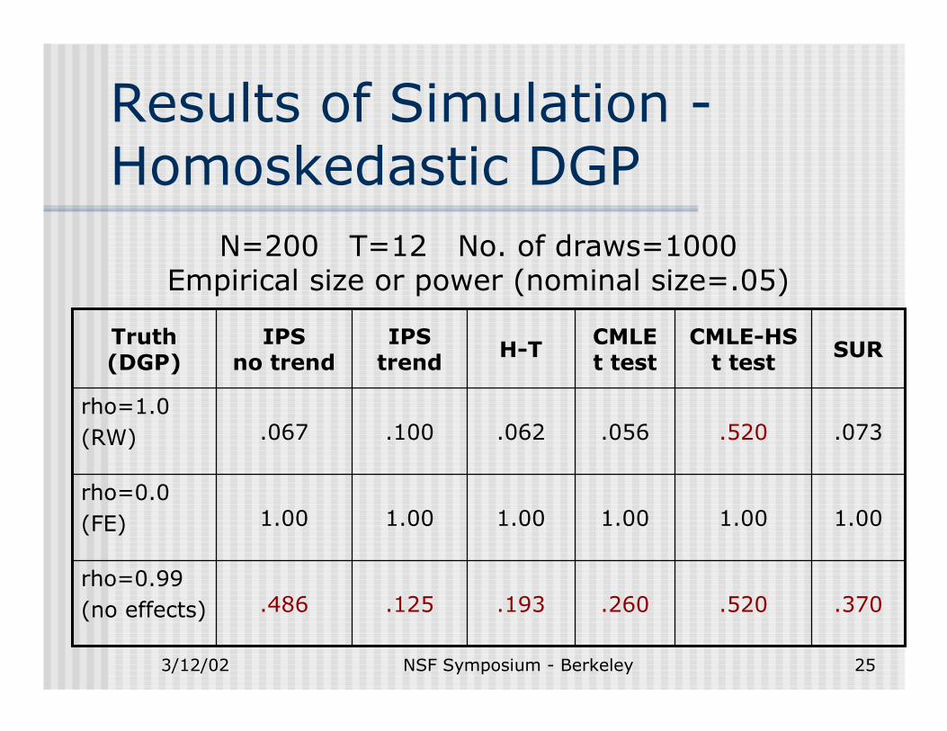
Results of Simulation -Homoskedastic DGP

N=200 T=12 No. of draws=1000Empirical size or power (nominal size=.05)

.260

1.00

.056

CMLE t test

.125

1.00

.100

IPStrend

.370.520.193.486rho=0.99(no effects)

1.001.001.001.00rho=0.0(FE)

.073.520.062.067rho=1.0(RW)

SURCMLE-HS t testH-TIPS

no trendTruth (DGP)


Results of Simulation -Heteroskedastic DGP

N=200 T=12 No. of draws=1000Empirical size or power (nominal size=.05)

.390

1.00

.200

CMLE t test

.240

1.00

.050

IPStrend

.303.550.369.125rho=0.99(no effects)

1.001.001.001.00rho=0.0(FE)

.124.450.210.090rho=1.0(RW)

SURCMLE-HS t testH-TIPS

no trendTruth (DGP)


Results of Unit Root TestsSeries with unit roots

US only

--

US only

US,F,J

US,J

IPSno

trend

--

--

US only

US,F

US,F,J

CMLE

------US,JCash flow

--------Investment

--US,F,JUS onlyUS,F,JR&D

J onlyUS,F,JUS,F,JUS,F,JEmployment

J onlyUS,F,JUS,F,JUS,F,JSales

SURCMLE with HSHT

IPSwith trend


Conclusions! A model with a very large autoregressive coefficient and

no level fixed effect may be a good description of these data – the substantive implication is that we use the initial condition rather than a permanent “effect” to describe differences across firms.

! CML estimation is feasible and may be a useful estimator in the cases where we cannot use the SUR idea.

! Next steps:! Heteroskedastic-consistent standard errors to correct size in

CMLE-HS, etc.! Further exploration of heterogeneous trends.! Modeling a more complex AR process for our data with

heteroskedasticity but no fixed effects.


Trends – real and simulated data

-0.20 -0.15 -0.10 -0.05 0.00 0.05 0.10 0.15 0.20 0.25 0.30

1

2

3

4

5

6

7

8

Estimated time trend


Intercepts – real and simulated data

-4 -3 -2 -1 0 1 2 3 4 5 6 7

0.05

0.10

0.15

0.20

0.25

0.30

0.35

0.40

Estimated Intercept

Documents

Testing for Unit Roots in Panel Databhhall/papers... · Panel Data: An Exploration Using Real and Simulated Data Bronwyn H. HALL UC Berkeley, Oxford University, and NBER Jacques MAIRESSE