Testing Equality of Several Correlation Matrices · Revista Colombiana de Estadística Diciembre2013,volumen36,no.2,pp.237a258 Testing Equality of Several Correlation Matrices Prueba

Revista Colombiana de EstadísticaDiciembre 2013, volumen 36, no. 2, pp. 237 a 258

Testing Equality of Several Correlation Matrices

Prueba de igualdad de varias matrices de correlación

Arjun K. Gupta1,a, Bruce E. Johnson2,b, Daya K. Nagar3,c

1Department of Mathematics and Statistics, Bowling Green State University,Bowling Green, USA

2Experient Research Group, Severna Park, USA3Instituto de Matemáticas, Facultad de Ciencias Exactas y Naturales, Universidad

de Antioquia, Medellín, Colombia

Abstract

In this article we show that the Kullback’s statistic for testing equalityof several correlation matrices may be considered a modified likelihood ratiostatistic when sampling from multivariate normal populations. We derivethe asymptotic null distribution of L∗ in series involving independent chi-square variables by expanding L∗ in terms of other random variables andthen inverting the expansion term by term. An example is also given toexhibit the procedure to be used when testing the equality of correlationmatrices using the statistic L∗.

Key words: Asymptotic null distribution, Correlation matrix, Covariancematrix, Cumulants, Likelihood ratio test.

Resumen

En este artículo se muestra que el estadístico L∗ de Kullback, para probarla igualdad de varias matrices de correlación, puede ser considerado como unestadístico modificado del test de razón de verosimilitud cuando se muestreanpoblaciones normales multivariadas. Derivamos la distribución asintóticanula de L∗ en series que involucran variables independientes chi-cuadrado,mediante la expansión de L∗ en términos de otras variables aleatorias yluego invertir la expansión término a término. Se da también un ejemplopara mostrar el procedimiento a ser usado cuando se prueba igualdad dematrices de correlación mediante el estadístico L∗.

Palabras clave: distribución asintótica nula, matriz de correlación, matrizde covarianza, razón de verosimilitud.

aProfessor. E-mail: [email protected]. E-mail: [email protected]. E-mail: [email protected]

237

238 Arjun K. Gupta, Bruce E. Johnson & Daya K. Nagar

1. Introduction

The correlation matrix is one of the foundations of factor analysis and hasfound its way into such diverse areas as economics, medicine, physical scienceand political science. There is a fair amount of literature on testing propertiesof correlation matrices. Tests for certain structures in a correlation matrix havebeen proposed and studied by several authors, e.g, see Aitkin, Nelson, and Rein-furt (1968), Gleser (1968), Aitkin (1969), Modarres (1993), Kullback (1997) andSchott (2007). In a series of papers, Konishi (1978, 1979a, 1979b) has developedasymptotic expansions of correlation matrix and applied them to various problemsof multivariate analysis. The exact distribution of the correlation matrix, whensampling from a multivariate Gaussian population, is derived in Ali, Fraser andLee (1970) and Gupta and Nagar (2000).

If the covariance matrix of α-th population is given by Σα and ∆α is a diagonalmatrix of standard deviations for the population α, then Pα = ∆−1α Σα∆−1α is thecorrelation matrix for the population α. The null hypothesis that all k populationshave the same correlation matrices may be stated as H : P1 = · · · = Pk.

Let the vectors xα1,xα2, . . . ,xαNα be a random sample of size Nα = nα + 1for α = 1, 2, . . . , k from k multivariate populations of dimensionality p. Further,we assume the independence of these k samples. Let xα =

∑Nαi=1 xαi/Nα, Aα =∑Nα

i=1(xαi−xα)(xαi−xα)′ and Sα = Aα/Nα. Further, letDα be a diagonal matrixof the square roots of the diagonal elements of Sα. The sample correlation matrixRα is then defined by Rα = D−1α SαD

−1α . Let n =

∑kα=1 nα and R =

∑kα=1 nαRα.

Kullback (1967) derived the statistic L∗ =∑kα=1 nα ln{det(R)/ det(Rα)} for

testing the equality of k correlation matrices based on samples from multivariatepopulations. This statistic was later examined by Jennrich (1970) who observedthat the statistic proposed by Kullback failed to have chi-square distribution as-cribed to it. For further results on this topic the reader is referred to Browne (1978)and Modarres and Jernigan (1992).

Although the Kullback’s statistic L∗ is not equal to the modified likelihood ratiocriterion, we here show that it may be considered an approximation of the modifiedlikelihood ratio statistic when sampling from multivariate normal populations.

In Section 2, we show that Kullback’s statistic can be viewed as an approxima-tion of the modified likelihood ratio statistic based on samples from multivariatenormal populations. Section 3 deals with some preliminary results and definitionswhich are used in subsequent sections. In sections 4 and 5, we obtain asymptoticnull distribution of L∗ by expanding L∗ in terms of other random variables andthen inverting the expansion term by term. Finally, in Section 6, an exampleis given to demonstrate the procedure to be used when testing the equality ofcorrelation matrices using the statistic L∗. Some results on matrix algebra anddistribution theory are given in the Appendix.

Revista Colombiana de Estadística 36 (2013) 237–258

Testing Equality of Several Correlation Matrices 239

2. The Test Statistic

In this section, we give an approximation of the likelihood ratio test statisticλ for testing equality of correlation matrices of several multivariate Gaussian pop-ulations. The test statistic λ was derived and studied by Cole (1968a, 1968b)in two unpublished technical reports (see Browne 1978, Modarres and Jerni-gan 1992, 1993). However, these reports are scarcely available, and therefore thesake of completeness and for a better understanding it seems appropriate to firstgive a concise step-by-step derivation of the test statistic λ.

If the underlying populations follow multivariate normal distributions, thenthe likelihood function based on the k independent samples, when all parametersare unrestricted, is given by

L(µ1, . . . ,µk,Σ1, . . . ,Σk)

=

k∏α=1

[(2π)pNα/2 det(Σα)Nα/2

]−1× exp

[−1

2

k∑α=1

tr(Σ−1α Aα

)− 1

2

k∑α=1

tr{

Σ−1α (xα − µα)(xα − µα)′}]

where for α = 1, . . . , k we have µα ∈ Rp and Σα > 0. It is well known that for anyfixed value of Σα the likelihood function is maximized with respect to the µα’swhen µα = xα.

Let ∆α be a diagonal matrix of standard deviations for the population α.Further, let Pα = ∆−1α Σα∆−1α be the population correlation matrix for the pop-ulation α. The natural logarithm of the likelihood function, after evaluation atµα = xα, may then be written as

ln[L(x1, . . . , xk,∆1P1∆1, . . . ,∆kPk∆k)]

= −1

2Np ln(2π)− 1

2

k∑α=1

Nα ln[det(Pα∆2α)]− 1

2

k∑α=1

tr(NαP−1α GαRαGα)

where N =∑kα=1Nα and Gα = ∆−1α Dα. Further, when the parameters are

unrestricted, the likelihood function L(x1, . . . ,xk,∆1P1∆1, . . . ,∆kPk∆k) is max-imized when − ln[det(Pα∆2

α)] − tr(P−1α GαRαGα

)is maximized for each α. This

is true when

ln[det(Pα∆2α)] + tr

(P−1α GαRαGα

)= ln[det(∆αPα∆α)] + tr

(∆−1α P−1α ∆−1α DαRαDα

)is minimized for each α. This is achieved when ∆αPα∆α = DαRαDα. From thisit follows that the maximum value of L(x1, . . . ,xk,∆1P1∆1, . . . ,∆kPk∆k), whenthe parameters are unrestricted, is given by



ln[L(x1, . . . , xk, D1R1D1, . . . , DkRkDk)]

= −1

2Np[ln(2π) + 1]− 1

2

k∑α=1

Nα ln[det(RαD2α)]. (1)

Let P be the common value of the population correlation matrices under the nullhypothesis of equality of correlation matrices. The reduced parameter space forthe covariance matrices is the set of all covariance matrices that may be writtenas ∆αP where P is a correlation matrix and ∆α is a diagonal matrix with positiveelements on the diagonal. The restricted log likelihood function is written as

ln[L(x1, . . . , xk,∆1P, . . . ,∆kP )]

= −1

2Np ln(2π)− 1

2

k∑α=1

Nα ln[det(P∆2α)]− 1

2

k∑α=1

Nα tr(P−1GαRαGα

).

Let P−1 = (ρij). Since ∆α is a diagonal matrix,

ln[det(∆α)2] = 2 ln[det(∆α)] = 2 ln

[p∏i=1

σαii

]= 2

p∑i=1

ln(σαii)

Also, since Gα = ∆−1α Dα is a diagonal matrix, we have

tr(P−1GαRαGα

)=

p∑i=1

p∑j=1

ρijgαjrαijgαi

Thus,

ln[L(x1, . . . , xk,∆1P, . . . ,∆kP )]

= −1

2Np ln(2π)− 1

2

k∑α=1

Nα

p∑i=1

ln(σαii)−1

2

k∑α=1

Nα ln[det(P )]

− 1

2

k∑α=1

Nα

p∑i=1

p∑j=1

ρijgαjrαijgαi

Since, gαi = sαii/σαii, differentiation of ln[L(x1, . . . ,xk,∆1P, . . . ,∆kP )] with re-spect to σαii yields

∂

∂σαiiln[L(x1, . . . ,xk,∆1P, . . . ,∆kP )] = − Nα

2σαii+

Nα2σαii

p∑j=1

gαigαjρijrαij

Further, setting this equal to zero gives∑pj=1 gαigαjρ

ijrαij−1 = 0. Differentiatingln[L(x1, . . . ,xk,∆1P, . . . ,∆kP )] with respect to the matrix P using Lemma 6, weobtain

∂

∂Pln[L(x1, . . . ,xk,∆1P, . . . ,∆kP )] = −1

2NP−1 +

1

2

k∑α=1

NαP−1GαRαGαP

−1



Setting this equal to zero, multiplying by 2, pre and post multiplying by P anddividing by N gives P =

∑kα=1NαGαRαGα/N so that

∑kα=1Nαg

2αi/N = 1.

The likelihood ratio test statistic λ for testing H : P1 = · · · = Pk is now derivedas

λ =

k∏α=1

det(RαD2α)Nα/2

det(P ∆2α)Nα/2

where P and ∆2α are solutions of P =

∑kα=1Nα∆−1α Sα∆−1α /N and

∑pj=1 ρ

ijsαij−1 = 0, i = 1, . . . , p, respectively.

To obtain an approximation of the likelihood ratio statistic we replace σαiiby its consistent estimator σαii. Then, it follows that gαii = sαii/σαii andGα = diag(gα1, . . . , gαp), and the estimator of P is given by P =

∑kα=1NαGαRα

Gα/N . Thus, an approximation of the maximum of ln[L(x1, . . . ,xk,∆1P, . . . ,∆kP )]is given as

− 1

2Np[ln(2π) + 1]− 1

2

k∑α=1

Nα ln[det(∆α)2]− 1

2N ln[det(P )] (2)

As the sample size goes to infinity, sαii/σαii converges in probability to 1 so thatGα converges in probability to Ip. This suggest further approximation of (2) as

− 1

2Np[ln(2π) + 1]− 1

2

k∑α=1

Nα ln[det(Dα)2]− 1

2N ln

[det

(k∑

α=1

NαNRα

)](3)

Now, using (1) and (3), the likelihood ratio statistic is approximated as

λ =

∏kα=1 det(Rα)Nα/2

det(∑kα=1NαRα/N)N/2

(4)

Further, replacing Nα by nα above, an approximated modified likelihood ratiostatistic is derived as

M =

∏kα=1 det(Rα)nα/2

det(∑kα=1 nαRα/n)n/2

=

∏kα=1 det(Rα)nα/2

det(R)n/2(5)

Since −2 lnM =∑kα=1 nα ln{det(R)/ det(Rα)} = L∗, the statistic proposed by

Kullback may be thought of as an approximated modified likelihood ratio statistic.

3. Preliminaries

Let the vectors xα1, . . . ,xαNα be a random sample of size nα for α = 1, . . . , kfrom k multivariate populations of dimensionality p and finite fourth moments.The characteristic function for the population α is given by φ∗α(t) = E[exp(ι t′x)]



where ι =√−1 and t = (t1, . . . , tp)

′. The log characteristic function for populationα may be written as

ln[φ∗α(t)] =

∞∑r1+···+rp=1

κ∗α(r1, . . . , rp)

p∏j=1

(ιtj)rj

rj !, rj ∈ I+ (6)

where I+ is the set of non-negative integers. The cumulants of the distribution arethe coefficients κ∗α(r1, . . . , rp). If r1 + · · ·+ rp = m, then the associated cumulantis of order m. The relationship between the cumulants of a distribution and thecharacteristic function provide a convenient method for deriving the asymptoticdistribution of statistic whose asymptotic expectations can be derived.

The cumulants of order m are functions of the moments of order m or lower.Thus if the mth order moment is finite, so is the mth order cumulant. Let µi =E(Xi), µij = E(XiXj), µijk = E(XiXjXk), and µijk` = E(XiXjXkX`) and κi,κij , κijk, and κijk` be the corresponding cumulants. Then, Kaplan (1952) givesthe following relationship:

κi = µi,

κij = µij − µiµj ,κijk = µijk − (µiµjk + µjµik + µkµij) + 2µiµjµk,

κijk` = µijk` −4∑µiµjk` −

3∑µijµk` + 2

6∑µiµjµk` − 6µiµjµkµ`

where the summations are over the possible ways of grouping the subscripts, andthe number of terms resulting is written over the summation sign.

Define the random matrix Vα as

Vα =√nα

(1

nα∆−1α Aα∆−1α − Pα

)(7)

Then, the random matrices V (0)α , V (1)

α and V (2)α are defined as

V (0)α = diag(vα11, vα22, . . . , vαpp) (8)

V (1)α = Vα −

1

2V (0)α Pα −

1

2PαV

(0)α (9)

and

V (2)α =

1

4V (0)α PαV

(0)α − 1

2VαV

(0)α − 1

2V (0)α Vα +

3

8(V (0)α )2Pα +

3

8Pα(V (0)

α )2 (10)

Konishi (1979a, 1979b) has shown that

Rα = Pα +1√nαV (1)α +

1

nαV (2)α +Op(n

−3/2α )

The pooled estimate of the common correlation matrix is

R =

k∑α=1

ωαRα



so thatR = P +

1√nV

(1)+

1

nV

(2)+Op(n

−3/2)

where ωα = nα/n, P =∑kα=1 ωαPα, V

(1)=

∑kα=1

√ωα V

(1)α and

V(2)

=∑kα=1 V

(2)α . The limiting distribution of Vα =

√nα(∆−1α Aα∆−1α /nα − Pα

)is normal with means 0 and covariances that depend on the fourth order cumulantsof the parent population (Anderson 2003, p. 88).

Since ∆α is a diagonal matrix of population standard deviations, ∆−1α xα1, . . . ,∆−1α xαNα may be thought of as Nα observations from a population with finitefourth order cumulants and characteristic function given by

ln[φα(t)] =

∞∑r1+···+rp=1

κα(r1, . . . , rp)

p∏j=1

(ιtj)rj

rj !, rj ∈ I+ (11)

where the standardized cumulants, κα(r1, r2, . . . , rp), are derived from the expres-sion (6) as

κα(r1, r2, . . . , rp) =κ∗α(r1, r2, . . . , rp)

σα11χr1σα22χr2 · · ·σαppχrp

with χrj = 1 if rj = 0, χrj = 1/σ(α)jj if rj 6= 0 and Σ−1α = (σ(α)jj).K-statistics are unbiased estimates of the cumulants of a distribution, and

may be used to derive the moments of the statistics which are symmetric func-tions of the observations (Kendall and Stuart 1969). Kaplan (1952) gives a seriesof tensor formulaes for computing the expectations of various functions of thek-statistics associated with a sample of size N from a multivariate population.For the definition of the k-statistics, let N (r) = N(N − 1) · · · (N − r + 1).

If si1i2···i` denotes the product Xi1Xi2 · · ·Xi` summed over the sample, thetensor formulae for the k-statistics may be shown to be as follows:

ki =siN, kij =

Nsij − sisjN (2)

, kijk =N2sijk −N

3∑sisjk + 2sisjsk

N (3)

kijk` =N(N + 1)(Nsijk` −

4∑sisjk`)−N (2)

3∑sijsk` + 2N

6∑sisjsk` − 6sisjsks`

N (4)

κ(ab, ij) = E[(kab − κab)(kij − κij)]

=κabijN

+κaiκbj + κajκbi

N − 1

κ(ab, ij, pq) = E[(kab − κab)(kij − κij)(kpq − κpq)]

=κabijpqN2

+

12∑ κabipκjqN(N − 1)

+

4∑ (N − 2)κaipκbjqN(N − 1)2

+

8∑ κaiκbpκjq(N − 1)2



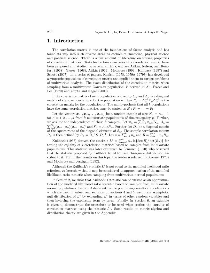
The summations are over the possible ways of grouping the subscripts, and thenumber of terms resulting is written over the summation sign.

The matrix Vα is constructed from observations from the standardized distri-bution so that vαij =

√nα(kαij − ραij) where kαij is the related k-statistic for

standardized population α. Kaplan’s formulae may be applied to derive the fol-lowing expressions for the expectations of elements of the matrices Vα (note thatκαij = ραij). We obtain

E(vαij) = 0

E(vαijvαk`) = καijk` + ραikραj` + ραi`ραjk +O(n−1α )

and

E(vαijvαk`vαab) =1√nα

[καijkàb +

12∑καijkaρα`b +

4∑καikaκαj`b

+

8∑ραikραjaρα`b

]+O(n−3/2α )

The random matrices V (0)α , V (1)

α and V (2)α are defined in (8), (9), and (10), respec-

tively. The expectations associated with these random matrices are given as

E(v(1)αij) = 0

E(v(2)αij) =

1

4ραijκαiijj −

1

2(καiiij + καijjj) +

3

8ραij(καiiii + καjjjj)

+1

2(ρ3αij − ραij) +O(n−1α )

E(v(1)αijv

(1)αk`) = καijk` −

1

2(ραijκαiik` + ραijκαjjk` + ραk`καijkk + ραk`καij``)

+1

4ραijραk`(καiikk + καii`` + καjjkk + καjj``)

− (ραk`ραikραjk + ραk`ραi`ραj` + ραijραikραi` + ραijραjkραj`)

+1

2ραijραk`(ρ

2αik + ρ2αi` + ρ2αjk + ρ2αi`)

+ (ραikραj` + ραi`ραjk) +O(n−1α ) (12)

and

E(v(1)αijv

(1)αk`v

(1)αab) =

1√nα

(tα1 −

1

2tα2 +

1

4tα3 −

1

8tα4

)+O(n−3/2α )

where

tα1 = καijkàb +

12∑καijkaκα`b +

4∑καikaκαi`b +

8∑ραikραjaρα`b



tα2 =

3∑ραij

[καiikàb + καjjkà +

12∑(καiika + καjjka)

+

3∑(καikaκαi`b + καjkaκαj`b) +

8∑(ραikραiaρα`b + ραjkραjaρα`b)

]

tα3 =

3∑ραijραk`

[καiikkab + καii`àb + καjjkkab + καjj`àb

+

12∑(καiikaραkb + καiiàρα`b + καjjkaραkb + καjjàρα`b)

+

3∑(καikaκαikb + καiàκαi`b + καjkaκαjkb + καjàκαj`b)

+

8∑(ραikραiaραbk + ραi`ραiaρα`b + ραjkραjaραbk + ραj`ραjaρα`b)

]and

tα4 = ραijραk`ραab

8∑[καiikkaa +

12∑(καiikaραka) +

3∑(καikaκαikb)

+

8∑(ραikραiaραka)

]Lemma 1. The diagonal elements of V (1)

α are zero.

Proof . Using (9) and the fact that V (0)α is a diagonal matrix, we have

v(1)αij = vαij −

1

2ραij(vαii + vαjj)

The result follows by taking j = i above and noting that diagonal elements of Pαare 1.

Lemma 2. The diagonal elements of V (2)α are zero.

Proof . Using (10) and the fact that V (0)α is a diagonal matrix, we get

v(2)αij =

1

4v(0)αiiραijv

(0)αjj −

1

2vαij(vαjj + vαii) +

3

8ραij(v

2αii + v2αjj)

The result follows by substituting j = i above and observing that ραii = 1.

4. Asymptotic Expansion of L∗

In order to derive the asymptotic distribution for L∗ the statistic is first ex-panded in terms of other random variables (see Konishi and Sugiyama 1981).



The statistic L∗ may be written as L∗ = ng(R1 . . . , Rk) where g(R1, . . . , Rk) =

ln[det(R)]−∑kα=1 ωα ln[det(Rα)]. Let

Bα =1√nαP−1α V (1)

α +1

nαP−1α V (2)

α

Since, Pα, V(1)α and V (2)

α are all positive definite, so is Bα. This insures that theeigenvalues of Bα exist and are positive. Also, as nα becomes large, the elementsin Bα become small so that the characteristic roots may be assumed to be lessthan one. Using Lemma 5,

ln[det(Rα)] = ln[det(Pα + PαBα)] +Op(n−3/2α )

= ln[det(Pα)] + tr(Bα)− 1

2tr(BαBα) +Op(n

−3/2α )

Now, BαBα = n−1α P−1α V(1)α P−1α V

(1)α +Op(n

−3/2α ) so that

ln[det(Rα)] = ln[det(Pα)] +1√nα

tr(P−1α V (1)α ) +

1

nαtr(P−1α V (2)

α )

− 1

2nαtr(P−1α V (1)

α P−1α V (1)α

)+Op(n

−3/2α )

A similar expansion for ln[det(R)] may be obtained by defining B by

B =1√n

k∑α=1

√ωαP

−1V (1)α +

1

n

k∑α=1

P−1V (2)α

Then

ln[det(R)] = ln[det(P + PB)] +Op(n−3/2)

= ln[det(P )] + tr(B)− 1

2tr(BB) +Op(n

−3/2)

Since BB = n−1∑kα=1

∑kβ=1

√ωαωβP

−1V

(1)α P

−1V

(1)β +Op(n

−3/2),

ln[det(R)] = ln[det(P )] +1√n

k∑α=1

√ωα tr(P

−1V (1)α ) +

1

n

k∑α=1

tr(P−1V (2)α )

− 1

2n

k∑α=1

k∑β=1

√ωαωβ tr(P

−1V (1)α P

−1V

(1)β ) +Op(n

−3/2)

Combining these expressions yields

g(R1, . . . , Rk) = ln[det(P )]−k∑

α=1

ωα ln[det(Pα)] +1√n

k∑α=1

√ωα tr(HαV

(1)α )

+1

n

k∑α=1

tr(HαV(2)α ) +

1

2

k∑α=1

ωαnα

tr(P−1α V (1)α P−1α V (1)

α )



− 1

2n

k∑α=1

k∑β=1

√ωαωβ tr(P

−1V (1)α P

−1V

(1)β ) +Op(n

−3/2)

where Hα = (hαij) = (P−1−P−1α ) = H ′α. Let G(R1, . . . , Rk) =

√n[g(R1, . . . , Rk)

−g(P1, . . . , Pk)]. Then, since√n(ωα/nα) = (

√n)−1, we obtain

G(R1, . . . , Rk) =

k∑α=1

√ωα tr(HαV

(1)α ) +

1√n

k∑α=1

tr(HαV(2)α )

+1

2√n

k∑α=1

tr(P−1α V (1)α P−1α V (1)

α )

− 1

2√n

k∑α=1

k∑β=1

√ωαωβ tr(P

−1V (1)α P

−1V

(1)β ) +Op(n

−1) (13)

Theorem 1. The expression G(R1, . . . , Rk) may be written as

G(R1, . . . , Rk) =

k∑α=1

∑i<j

√ωα hαijv

(1)αij +

1√n

k∑α=1

∑i<j

hαijv(2)αij

+1√n

k∑α=1

∑i<j

∑k<`

qα(ij, k`)v(1)αijv

(1)αk`

− 1√n

k∑α=1

k∑β=1

∑i<j

∑k<`

√ωαωβ q(ij, k`)v

(1)αijv

(1)βk` +Op(n

−1)

where P−1α = (ρijα ), P−1

= (ρij), hαij = 2(ρij − ρijα ), qα(ij, k`) = ρi`αρjkα +

ρikα ρj`α and q(ij, k`) = ρi`ρjk + ρikρj`.

Proof . Using results on matrix algebra, we have

k∑α=1

√ωα tr(HαV

(1)α ) =

k∑α=1

√ωα

p∑i=1

p∑j=1

hαjiv(1)αij

and since Hα is symmetric, application of Lemma 3 yields

k∑α=1

√ωα tr(HαV

(1)α ) =

k∑α=1

√ωα∑i<j

(hαji + hαij)v(1)αij =

k∑α=1

√ωα∑i<j

hαijv(1)αij

In an entirely similar manner,

k∑α=1

tr(HαV(2)α ) =

k∑α=1

∑i<j

hαijv(2)αij



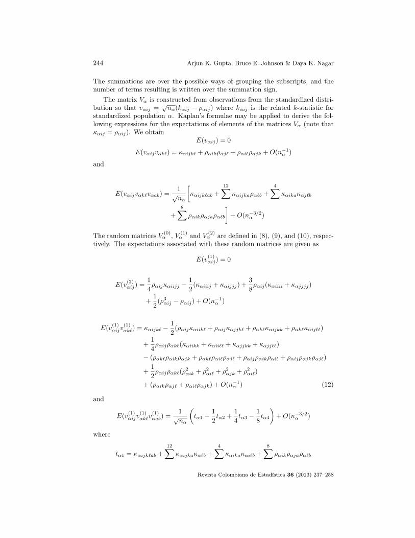
Using Lemma 4, results on matrix algebra and the symmetry of V (1)α , we have

1

2

k∑α=1

tr(P−1α V (1)α P−1α V (1)

α )

=1

2

k∑α=1

p∑i=1

p∑j=1

p∑k=1

p∑`=1

ρi`αρjkα v

(1)αijv

(1)αk`

=1

2

k∑α=1

∑i<j

∑k<`

(ρi`αρjkα + ρj`α ρ

ikα + ρikα ρ

j`α + ρi`αρ

jkα )v

(1)αijv

(1)αk`

=

k∑α=1

∑i<j

∑k<`

qα(ij, k`)v(1)αijv

(1)αk`

In a similar manner,

1

2

k∑α=1

k∑β=1

√ωαωβ tr(P

−1V (1)α P

−1V

(1)β )

=

k∑α=1

k∑β=1

∑i<j

∑k<`


(1)αijv

(1)βk`

Combining these expansions in (13) completes the proof.

Corollary 1. In the special case p = 2, G(R1, . . . , Rk) may be written as

G(R1, . . . , Rk) = 2

k∑α=1

√ωα

(ρα

1− ρ2α− ρ

1− ρ2

)v(1)α12

+2√n

k∑α=1

(ρα

1− ρ2α− ρ

1− ρ2

)v(2)α12 +

1√n

k∑α=1

1 + ρ2α(1− ρ2α)2

(v(1)α12)2

− 1√n

k∑α=1

k∑β=1

1 + ρ2

(1− ρ2)2v(1)α12v

(1)β12 +Op(n

−1).

Proof . For p = 2,∑i<j consists of single term corresponding to i = 1, j = 2.

Also, Pα =( 1 ραρα 1

)so that P−1α = (1 − ρ2α)−1

( 1 −ρα−ρα 1

). Similarly, P

−1=

(1 − ρ2)−1(

1 −ρ−ρ 1

). Thus, the off diagonal element of Hα is given by ρα(1 −

ρ2α)−1 − ρ(1 − ρ2)−1. Further, qα(12, 12) = ρ12α ρ21α + ρ11α ρ

22α = (1 + ρ2α)/(1 − ρ2α)2

and q(12, 12) = (1 + ρ2)/(1− ρ2)2. The result follows by using these values in thetheorem.

5. Asymptotic Null Distribution of L∗

In this section we derive asymptotic distribution of the statistic L∗ when thenull hypothesis is true.



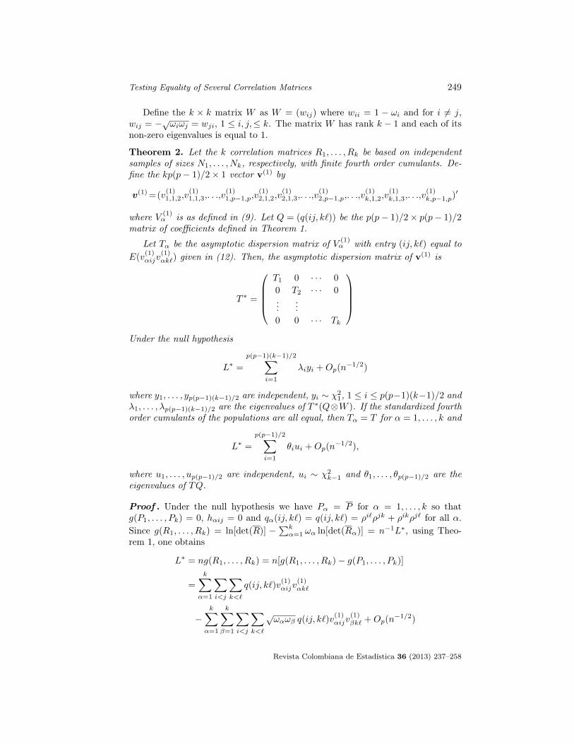
Define the k × k matrix W as W = (wij) where wii = 1 − ωi and for i 6= j,wij = −√ωiωj = wji, 1 ≤ i, j,≤ k. The matrix W has rank k − 1 and each of itsnon-zero eigenvalues is equal to 1.

Theorem 2. Let the k correlation matrices R1, . . . , Rk be based on independentsamples of sizes N1, . . . , Nk, respectively, with finite fourth order cumulants. De-fine the kp(p− 1)/2× 1 vector v(1) by

v(1) =(v(1)1,1,2,v

(1)1,1,3,. . .,v

(1)1,p−1,p,v

(1)2,1,2,v

(1)2,1,3,. . .,v

(1)2,p−1,p,. . .,v

(1)k,1,2,v

(1)k,1,3,. . .,v

(1)k,p−1,p)

′

where V (1)α is as defined in (9). Let Q = (q(ij, k`)) be the p(p− 1)/2× p(p− 1)/2

matrix of coefficients defined in Theorem 1.

Let Tα be the asymptotic dispersion matrix of V (1)α with entry (ij, k`) equal to

E(v(1)αijv

(1)αk`) given in (12). Then, the asymptotic dispersion matrix of v(1) is

T ∗ =

T1 0 · · · 0

0 T2 · · · 0...

...0 0 · · · Tk

Under the null hypothesis

L∗ =

p(p−1)(k−1)/2∑i=1

λiyi +Op(n−1/2)

where y1, . . . , yp(p−1)(k−1)/2 are independent, yi ∼ χ21, 1 ≤ i ≤ p(p−1)(k−1)/2 and

λ1, . . . , λp(p−1)(k−1)/2 are the eigenvalues of T ∗(Q⊗W ). If the standardized fourthorder cumulants of the populations are all equal, then Tα = T for α = 1, . . . , k and

L∗ =

p(p−1)/2∑i=1

θiui +Op(n−1/2),

where u1, . . . , up(p−1)/2 are independent, ui ∼ χ2k−1 and θ1, . . . , θp(p−1)/2 are the

eigenvalues of TQ.

Proof . Under the null hypothesis we have Pα = P for α = 1, . . . , k so thatg(P1, . . . , Pk) = 0, hαij = 0 and qα(ij, k`) = q(ij, k`) = ρi`ρjk + ρikρj` for all α.Since g(R1, . . . , Rk) = ln[det(R)] −

∑kα=1 ωα ln[det(Rα)] = n−1L∗, using Theo-

rem 1, one obtains

L∗ = ng(R1, . . . , Rk) = n[g(R1, . . . , Rk)− g(P1, . . . , Pk)]

=

k∑α=1

∑i<j

∑k<`

q(ij, k`)v(1)αijv

(1)αk`

−k∑

α=1

k∑β=1

∑i<j

∑k<`


(1)αijv

(1)βk` +Op(n

−1/2)



=

k∑α=1

k∑β=1

wαβ∑i<j

∑k<`

q(ij, k`)v(1)αijv

(1)βk` +Op(n

−1/2)

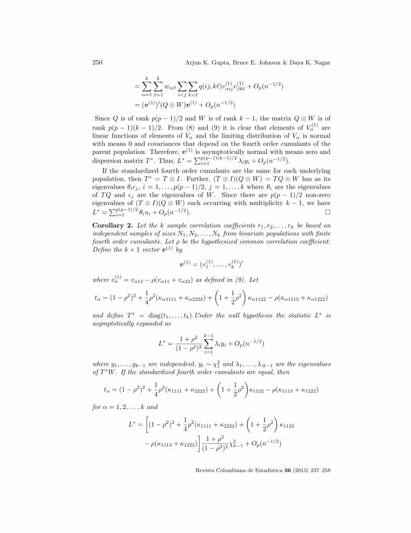
= (v(1))′(Q⊗W )v(1) +Op(n−1/2)

Since Q is of rank p(p − 1)/2 and W is of rank k − 1, the matrix Q ⊗W is ofrank p(p − 1)(k − 1)/2. From (8) and (9) it is clear that elements of V (1)

α arelinear functions of elements of Vα and the limiting distribution of Vα is normalwith means 0 and covariances that depend on the fourth order cumulants of theparent population. Therefore, v(1) is asymptotically normal with means zero anddispersion matrix T ∗. Thus, L∗ =

∑p(p−1)(k−1)/2i=1 λiyi +Op(n

−1/2).If the standardized fourth order cumulants are the same for each underlying

population, then T ∗ = T ⊗ I. Further, (T ⊗ I)(Q ⊗W ) = TQ ⊗W has as itseigenvalues θiεj , i = 1, . . . , p(p − 1)/2, j = 1, . . . , k where θi are the eigenvaluesof TQ and εj are the eigenvalues of W . Since there are p(p − 1)/2 non-zeroeigenvalues of (T ⊗ I)(Q ⊗W ) each occurring with multiplicity k − 1, we haveL∗ =

∑p(p−1)/2i=1 θiui +Op(n

−1/2).

Corollary 2. Let the k sample correlation coefficients r1, r2, . . . , rk be based onindependent samples of sizes N1, N2, . . . , Nk from bivariate populations with finitefourth order cumulants. Let ρ be the hypothesized common correlation coefficient.Define the k × 1 vector v(1) by

v(1) = (v(1)1 , . . . , v

(1)k )′

where v(1)α = vα12 − ρ(vα11 + vα22) as defined in (9). Let

tα = (1− ρ2)2 +1

4ρ2(κα1111 + κα2222) +

(1 +

1

2ρ2)κα1122 − ρ(κα1113 + κα1222)

and define T ∗ = diag(t1, . . . , tk).Under the null hypothesis the statistic L∗ isasymptotically expanded as

L∗ =1 + ρ2

(1− ρ2)2

k−1∑i=1

λiyi +Op(n−1/2)

where y1, . . . , yk−1 are independent, yi ∼ χ21 and λ1, . . . , λ,k−1 are the eigenvalues

of T ∗W . If the standardized fourth order cumulants are equal, then

tα = (1− ρ2)2 +1

4ρ2(κ1111 + κ2222) +

(1 +

1

2ρ2)κ1122 − ρ(κ1113 + κ1222)

for α = 1, 2, . . . , k and

L∗ =

[(1− ρ2)2 +

1

4ρ2(κ1111 + κ2222) +

(1 +

1

2ρ2)κ1122

− ρ(κ1113 + κ1222)

]1 + ρ2

(1− ρ2)2χ2k−1 +Op(n

−1/2)



Proof . As shown in Corollary 1, when p = 2, Q is a scalar. If ρ is the commoncorrelation coefficient, then Q = (1 + ρ2)/(1 − ρ2)2. The asymptotic variance ofv(1)α12 is given in (12). Upon simplification,

E(v(1)α12v

(1)α12) = tα = (1− ρ2)2 +

1

4ρ2(κα1111 + κα2222) +

(1 +

1

2ρ2)κα1122

− ρ(κα1113 + κα1222) +Op(n−1/2) (14)

so that T ∗ is the asymptotic covariance matrix of v(1). Further, T ∗(Q ⊗W ) =

[(1 + ρ2)/(1− ρ2)2]T ∗W . Thus L∗ = [(1 + ρ2)/(1− ρ2)2]∑k−1i=1 λiyi +Op(n

−1/2),where λi are the eigenvalues of T ∗W . If the standardized fourth order cumulantsare identical, T = tI, so that there is one eigenvalue of TQ with multiplicity k.This eigenvalue is merely t(1 + ρ2)/(1 − ρ2)2 and the result follows immediatelyfrom Theorem 2.

Corollary 3. Let the k sample correlation coefficients r1, r2, . . . , rk be based onindependent samples of sizes N1, N2, . . . , Nk from bivariate populations which areelliptically contoured with a common curtosis of 3κ and common correlation coef-ficient ρ. Then

L∗ =[(1− ρ2)2 + (1 + 2ρ2)κ

] 1 + ρ2

(1− ρ2)2χ2k−1 +Op(n

−1/2)

Proof . For elliptically contoured distributions (Muirhead 1982, Anderson 2003,Gupta and Varga 1993) the fourth order cumulants are such that κiiii = 3κiijj =3κ for i 6= j and all other cumulants are zero (Waternaux 1984). Substituting thisinto the expression for t in Corollary 2 yields t = (1−ρ2)2 +(1+2ρ2)κ. The resultthen follows from Corollary 2.

Corollary 4. Let the k sample correlation coefficients r1, . . . , rk be based on in-dependent samples of sizes N1, . . . , Nk from bivariate normal populations with acommon correlation coefficient ρ. Then

L∗ = (1 + ρ2)χ2k−1 +Op(n

−1/2)

Proof . Normal distributions are special case of elliptically contoured distribu-tions. The fourth order cumulants are all zero (Anderson 2003). The result followsby setting κ = 0 in Corollary 3.

6. An Example

This example is included to demonstrate the procedure to be used when testingthe equality of correlation matrices by using the statistic L∗. The data representrandom samples from three trivariate populations each with identical correlationmatrix P given by

P =

1.0 0.3 0.2

0.3 1.0 −0.3

0.2 −0.3 1.0



Since the statistic L∗ is an approximation of the modified likelihood ratio statisticfor samples from multivariate normal populations, it is particularly suited to pop-ulations that are near normal. The contaminated normal model has been chosento represent such a distribution.

Samples of size 25 from contaminated normal populations with mixing param-eter ε = 0.1 and σ = 2 were generated using the SAS system. These data aretabulated in Gupta, Johnson and Nagar (2012). The density of a contaminatednormal model is given by

φε(x, σ,Σ) = (1− ε)φ(x,Σ) + εφ(x, σΣ), σ > 0, 0 < ε < 1

where φ(x,Σ) is the density of a multivariate normal distribution with zero meanvector and covariance matrix Σ.

If the data were known to be from three normal populations all that wouldbe required at this point would be the sample sizes and the matrix of correctedsums of squares and cross products. A key element, however, of the modifiedlikelihood ratio procedure is that this assumption need not be made, but thefourth order cumulant must be estimated. To do this the k-statistics are calculatedusing Kaplan’s formulae summarized in Section 3. The computations are madeconsiderably easier by standardizing the data so that all of the first order sumsare zero.

The computation using original (or standardized) data yields the followingestimates of the individual correlation matrices:

R1 =

1.0000 0.5105 0.3193

0.5105 1.0000 −0.3485

0.3193 −0.3485 1.0000

, det(R1) = 0.4024

R2 =

1.0000 0.1758 0.2714

0.1758 1.0000 −0.2688

0.2714 −0.2688 1.0000

, det(R2) = 0.7975

R3 =

1.0000 0.2457 0.3176

0.2457 1.0000 −0.0331

0.3176 −0.0331 1.0000

, det(R3) = 0.8325

Since each sample is of size 25, ωi = 1/3 for i = 1, 2, 3 and the pooled correlationmatrix is merely the average of these three matrices:

R =

1.0000 0.3107 0.3028

0.3107 1.0000 −0.2168

0.3028 −0.2168 1.0000

, det(R) = 0.7240

The value of the test statistic is now easily calculated as

L∗ = 72 ln(0.7240)− 24[ln(0.4024) + ln(00.7975) + ln(0.8325)]

= 8.7473



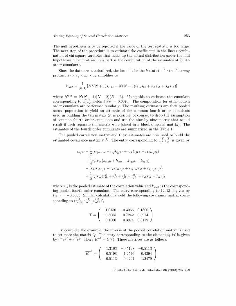
The null hypothesis is to be rejected if the value of the test statistic is too large.The next step of the procedure is to estimate the coefficients in the linear combi-nation of chi-square variables that make up the actual distribution under the nullhypothesis. The most arduous part is the computation of the estimates of fourthorder cumulants.

Since the data are standardized, the formula for the k-statistic for the four wayproduct xi × xj × xk × x` simplifies to

kijk` =1

N (4)[N2(N + 1)sijk` −N(N − 1)(sijsk` + siksj` + si`sjk)]

where N (4) = N(N − 1)(N − 2)(N − 3). Using this to estimate the cumulantcorresponding to x21x22 yields k1122 = 0.6670. The computation for other fourthorder cumulant are performed similarly. The resulting estimates are then pooledacross population to yield an estimate of the common fourth order cumulantsused in building the tau matrix (it is possible, of course, to drop the assumptionof common fourth order cumulants and use the nine by nine matrix that wouldresult if each separate tau matrix were joined in a block diagonal matrix). Theestimates of the fourth order cumulants are summarized in the Table 1.

The pooled correlation matrix and these estimates are now used to build theestimated covariance matrix V (1). The entry corresponding to v(1)ij v

(1)k` is given by

kijk` −1

2(rijkiik` + rijkjjk` + rk`kijkk + rk`kij``)

+1

4rijrk`(kiikk + kii`` + kjjkk + kjj``)

− (rk`rikrjk + rk`ri`rj` + rijrikri` + rijrjkrj`)

+1

2rijrk`(r

2ik + r2i` + r2jk + r2j`) + rikrj` + ri`rjk

where rij is the pooled estimate of the correlation value and kijk` is the correspond-ing pooled fourth order cumulant. The entry corresponding to 12, 13 is given byt12,13 = −0.3065. Similar calculations yield the following covariance matrix corre-sponding to (v

(1)α12, v

(1)α13, v

(1)α23)′,

T =

1.0150 −0.3065 0.1800

−0.3065 0.7242 0.3974

0.1800 0.3974 0.8179

To complete the example, the inverse of the pooled correlation matrix is used

to estimate the matrix Q. The entry corresponding to the element ij, k` is givenby rikrj` + ri`rjk where R−1 = (rij). These matrices are as follows:

R−1

=

1.3163 −0.5198 −0.5113

−0.5198 1.2546 0.4294

−0.5113 0.4294 1.2479



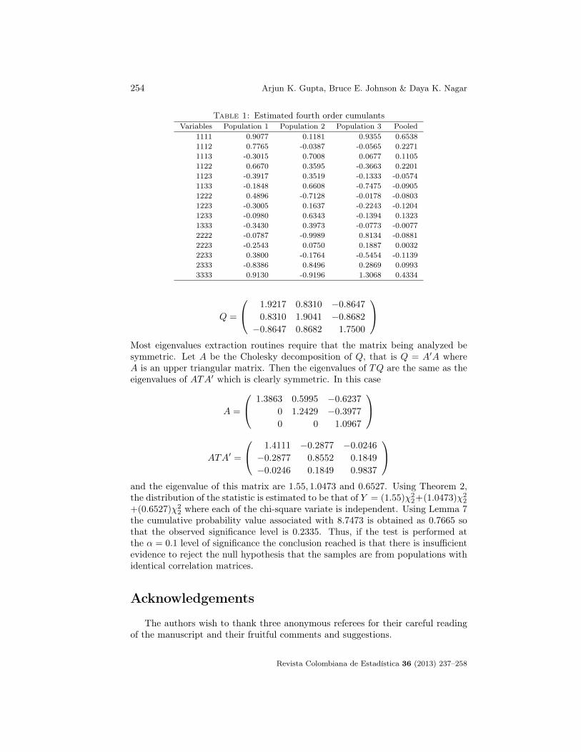
Table 1: Estimated fourth order cumulantsVariables Population 1 Population 2 Population 3 Pooled

1111 0.9077 0.1181 0.9355 0.65381112 0.7765 -0.0387 -0.0565 0.22711113 -0.3015 0.7008 0.0677 0.11051122 0.6670 0.3595 -0.3663 0.22011123 -0.3917 0.3519 -0.1333 -0.05741133 -0.1848 0.6608 -0.7475 -0.09051222 0.4896 -0.7128 -0.0178 -0.08031223 -0.3005 0.1637 -0.2243 -0.12041233 -0.0980 0.6343 -0.1394 0.13231333 -0.3430 0.3973 -0.0773 -0.00772222 -0.0787 -0.9989 0.8134 -0.08812223 -0.2543 0.0750 0.1887 0.00322233 0.3800 -0.1764 -0.5454 -0.11392333 -0.8386 0.8496 0.2869 0.09933333 0.9130 -0.9196 1.3068 0.4334

Q =

1.9217 0.8310 −0.8647

0.8310 1.9041 −0.8682

−0.8647 0.8682 1.7500

Most eigenvalues extraction routines require that the matrix being analyzed besymmetric. Let A be the Cholesky decomposition of Q, that is Q = A′A whereA is an upper triangular matrix. Then the eigenvalues of TQ are the same as theeigenvalues of ATA′ which is clearly symmetric. In this case

A =

1.3863 0.5995 −0.6237

0 1.2429 −0.3977

0 0 1.0967

ATA′ =

1.4111 −0.2877 −0.0246

−0.2877 0.8552 0.1849

−0.0246 0.1849 0.9837

and the eigenvalue of this matrix are 1.55, 1.0473 and 0.6527. Using Theorem 2,the distribution of the statistic is estimated to be that of Y = (1.55)χ2

2+(1.0473)χ22

+(0.6527)χ22 where each of the chi-square variate is independent. Using Lemma 7

the cumulative probability value associated with 8.7473 is obtained as 0.7665 sothat the observed significance level is 0.2335. Thus, if the test is performed atthe α = 0.1 level of significance the conclusion reached is that there is insufficientevidence to reject the null hypothesis that the samples are from populations withidentical correlation matrices.

Acknowledgements

The authors wish to thank three anonymous referees for their careful readingof the manuscript and their fruitful comments and suggestions.



[Recibido: junio de 2012 — Aceptado: julio de 2013

]References

Aitkin, M. (1969), ‘Some tests for correlation matrices’, Biometrika 56, 443–446.

Aitkin, M. A., Nelson, W. C. & Reinfurt, K. H. (1968), ‘Tests for correlationmatrices’, Biometrika 55, 327–334.

Ali, M. M., Fraser, D. A. S. & Lee, Y. S. (1970), ‘Distribution of the correlationmatrix’, Journal of Statistical Research 4, 1–15.

Anderson, T. W. (2003), An Introduction to Multivariate Statistical Analysis, Wi-ley Series in Probability and Statistics, third edn, Wiley-Interscience [JohnWiley & Sons], Hoboken, NJ.

Browne, M. W. (1978), ‘The likelihood ratio test for the equality of correlationmatrices’, The British Journal of Mathematical and Statistical Psychology31(2), 209–217.*http://dx.doi.org/10.1111/j.2044-8317.1978.tb00585.x

Cole, N. (1968a), The likelihood ratio test of the equality of correlation matrices,Technical Report 1968-65, The L. L. Thurstone Psychometric Laboratory,University of North Carolina, Chapel Hill, North Carolina.

Cole, N. (1968b), On testing the equality of correlation matrices, Technical Report1968-66, The L. L. Thurstone Psychometric Laboratory, University of NorthCarolina, Chapel Hill, North Carolina.

Gleser, L. J. (1968), ‘On testing a set of correlation coefficients for equality: Someasymptotic results’, Biometrika 55, 513–517.

Gupta, A. K., Johnson, B. E. & Nagar, D. K. (2012), Testing equality of severalcorrelation matrices, Technical Report 12-08, Department of Mathematicsand Statistics, Bowling Green State University, Bowling Green, Ohio.

Gupta, A. K. & Nagar, D. K. (2000), Matrix Variate Distributions, Vol. 104 ofChapman & Hall/CRC Monographs and Surveys in Pure and Applied Math-ematics, Chapman & Hall/CRC, Boca Raton, FL.

Gupta, A. K. & Varga, T. (1993), Elliptically Contoured Models in Statistics, Vol.240 of Mathematics and its Applications, Kluwer Academic Publishers Group,Dordrecht.*http://dx.doi.org/10.1007/978-94-011-1646-6

Jennrich, R. I. (1970), ‘An asymptotic χ2 test for the equality of two correlationmatrices’, Journal of the American Statistical Association 65, 904–912.

Kaplan, E. L. (1952), ‘Tensor notation and the sampling cumulants of k-statistics’,Biometrika 39, 319–323.



Kendall, M. G. & Stuart, A. (1969), The Advanced Theory of Statistics, Vol. 1 ofThird edition, Hafner Publishing Co., New York.

Konishi, S. (1978), ‘An approximation to the distribution of the sample correlationcoefficient’, Biometrika 65(3), 654–656.*http://dx.doi.org/10.1093/biomet/65.3.654

Konishi, S. (1979a), ‘Asymptotic expansions for the distributions of functions of acorrelation matrix’, Journal of Multivariate Analysis 9(2), 259–266.*http://dx.doi.org/10.1016/0047-259X(79)90083-6

Konishi, S. (1979b), ‘Asymptotic expansions for the distributions of statistics basedon the sample correlation matrix in principal component analysis’, HiroshimaMathematical Journal 9(3), 647–700.*http://projecteuclid.org/getRecord?id=euclid.hmj/1206134750

Konishi, S. & Sugiyama, T. (1981), ‘Improved approximations to distributions ofthe largest and the smallest latent roots of a Wishart matrix’, Annals of theInstitute of Statistical Mathematics 33(1), 27–33.*http://dx.doi.org/10.1007/BF02480916

Kullback, S. (1967), ‘On testing correlation matrices’, Applied Statistics 16, 80–85.

Kullback, S. (1997), Information Theory and Statistics, Dover Publications Inc.,Mineola, NY. Reprint of the second (1968) edition.

Modarres, R. (1993), ‘Testing the equality of dependent variances’, BiometricalJournal 35(7), 785–790.*http://dx.doi.org/10.1002/bimj.4710350704

Modarres, R. & Jernigan, R. W. (1992), ‘Testing the equality of correlation matri-ces’, Communications in Statistics. Theory and Methods 21(8), 2107–2125.*http://dx.doi.org/10.1080/03610929208830901

Modarres, R. & Jernigan, R. W. (1993), ‘A robust test for comparing correlationmatrices’, Journal of Statistical Computation and Simulation 43(3–4), 169–181.

Muirhead, R. J. (1982), Aspects of Multivariate Statistical Theory, John Wiley &Sons Inc., New York. Wiley Series in Probability and Mathematical Statistics.

Schott, J. R. (2007), ‘Testing the equality of correlation matrices when samplecorrelation matrices are dependent’, Journal of Statistical Planning and In-ference 137(6), 1992–1997.*http://dx.doi.org/10.1016/j.jspi.2006.05.005

Siotani, M., Hayakawa, T. & Fujikoshi, Y. (1985), Modern Multivariate StatisticalAnalysis: A Graduate Course and Handbook, American Sciences Press Se-ries in Mathematical and Management Sciences, 9, American Sciences Press,Columbus, OH.



Waternaux, C. M. (1984), ‘Principal components in the nonnormal case: The testof equality of q roots’, Journal of Multivariate Analysis 14(3), 323–335.*http://dx.doi.org/10.1016/0047-259X(84)90037-X

Appendix

Lemma 3. Let V = (vij) be a p× p symmetric matrix with zero on the diagonaland let C = (cij) be a p× p symmetric matrix. Then

tr(CV ) =

p∑i=1

p∑j=1

cijvij = 2∑i<j

cijvij

Proof . The proof is obtained by noting that vjj = 0 and cij = cji.

Lemma 4. Let Vα = (vαij) and Vβ = (vβij) be p × p symmetric matrices withzero on the diagonal. Then

p∑i=1

p∑j=1

p∑k=1

p∑`=1

cijk`vαijvβk` =∑i<j

∑k<`

(cijk` + cij`k + cjik` + cji`k)vαijvβk`.

Proof . Using Lemma 3, the sum may be written as

p∑i=1

p∑j=1

∑k<`

(cijk` + cij`k)vαijvβk`

The proof is obtained by applying Lemma 3 second time.

Lemma 5. Let A be a real symmetric matrix with eigenvalues that are less thanone in absolute value, then

− ln[det(I −A)] = tr(A) +1

2tr(A2) +

1

3tr(A3) + · · ·

Proof . See Siotani, Hayakawa and Fujikoshi (1985).

Lemma 6. Let R be a correlation of dimension p. Then

∂

∂Pln[detR] = R−1

and

∂

∂Ptr(R−1B) = R−1BR−1

where B is a symmetric non-singular matrix of order p.

Proof . See Siotani, Hayakawa and Fujikoshi (1985).



Lemma 7. Let Y1, Y2 and Y3 be independent random variables, Yi ∼ χ22, i = 1, 2, 3.

Define Y = α1Y1 + α2Y2 + α3Y3 where α1, α2 and α3 are constants, α1 > α2 >α3 > 0. Then, the cumulative distribution function FY (y) of Y is given by

FY (y) =

3∑i=1

Ci

[1− exp

(− y

2αi

)], y > 0,

where C1 = α21/(α1 − α3)(α1 − α2), C2 = −α2

2/(α2 − α3)(α1 − α2) andC3 = α2

3/(α2 − α3)(α1 − α3)

Proof . We get the desired result by inverting the moment generating functionMY (t) =

∑3i=1 Ci(1− 2αit)

−1, 2α1t < 1.


Documents

Testing Equality of Several Correlation Matrices · Revista Colombiana de Estadística Diciembre2013,volumen36,no.2,pp.237a258 Testing Equality of Several Correlation Matrices Prueba