Testing Efficient Risk Sharing with Heterogeneous Risk Preferences∗

Maurizio Mazzocco Shiv Saini

UCLA University of Wisconsin

Current Draft, January 2008. First Draft, October 2005.

Abstract

Previous papers have tested efficient risk sharing under the assumption of identical risk prefer-

ences. In this paper we show that, if in the data households have heterogeneous risk preferences,

the tests proposed in the past reject efficiency even if households share risk efficiently. To address

this issue we propose a method that enables one to test efficiency even when households have

different preferences for risk. The method is composed of three tests. The first one can be used to

determine whether in the data under investigation households have homogeneous risk preferences.

The second and third test can be used to evaluate efficient risk sharing when the hypothesis of

homogeneous risk preferences is rejected. We use this method to test efficient risk sharing in rural

India. Using the first test, we strongly reject the hypothesis of identical risk preferences. We then

test efficiency with and without the assumption of preference homogeneity. In the first case we

reject efficient risk sharing at the village and caste level. In the second case we still reject efficiency

at the village level, but we cannot reject this hypothesis at the caste level. This finding suggests

that the relevant risk-sharing unit in rural India is the caste and not the village.

1 Introduction

A good understanding of the degree of risk sharing that characterizes households in industrialized

and developing countries is important to answer policy questions. To see this consider for instance a

village in a developing country. The consumption pattern and hence the welfare of each individual

in the village is affected by a variety of idiosyncratic and aggregate shocks. Some examples of such

shocks are severe weather conditions, price fluctuations, health problems, unemployment spells, and∗We are grateful to Pierre-Andre Chiappori, Mariacristina De Nardi, Frederico Finan, James Heckman, Joseph Hotz,

John Kennan, Dennis Kristensen, Rodolfo Manuelli, Jack Porter, Bernard Salanie, Duncan Thomas, Jesus Fernandez-

Villaverde, James Walker, and participants at seminars at the Federal Reserve Bank of New York and Minneapolis,

Columbia University, Duke University, NYU, University of California at Los Angeles, University of California at San

Diego, University of California at Santa Cruz, University of Illinois at Urbana-Champaign, University of Western

Ontario, University of Wisconsin-Milwaukee, at the Conference on Macroeconomics of Imperfect Risk Sharing, at the

Society for Economic Dynamics, and at SITE for helpful comments.

1

USC FBE DEPT. MACROECONOMICS

presented by Maurizio MazzoccoFRIDAY, May 2, 20083:30 pm – 5:00 pm, Room: HOH-706

& INTERNATIONAL FINANCE WORKSHOP

crop diseases. Unless the households in the village can insure themselves against these shocks using

the existing institutions, individual consumption will fluctuate in response to them with detrimental

effects on individual welfare. The typical risk-sharing institutions available to households in rural

villages are gifts and transfers, borrowing from village lenders, saving and storage technologies, and the

diversification of crops. In addition to the existing institutions, the local and central government may

decide to provide additional insurance for instance by introducing new financial assets, by simplifying

the access to the existing financial markets, or by providing crop, health, and unemployment insurance.

A crucial step in evaluating whether there is scope for government reforms is the derivation of tests

that enable one to determine whether households are able to share risk efficiently using the existing

institutions. In the past three decades several papers have derived such tests and tested efficient risk

sharing in industrialized and developing countries. The papers in this literature have one common

feature. They assume that households have identical preferences for risk. The first contribution of the

present paper is to show that, if in the data the preferences for risk are heterogeneous, the tests used

in the past reject efficient risk sharing even if the households under investigation share risk efficiently.

The second contribution of this paper is to provide a method that enables one to test efficient risk

sharing even when households have heterogeneous preferences for risk. The method is composed of

three tests. The first one is a test of homogeneity in risk preferences. Using this test, the researcher can

determine whether the hypothesis of identical risk preferences is rejected for the group of households

that is being analyzed. If this hypothesis is not rejected one can use the tests proposed in the past.

If this hypothesis is rejected, however, new tests are required that allow for preference heterogeneity.

The second and third test derived here enable one to test efficient risk sharing when the null of

identical risk preferences is violated.

The method that we propose is based on a new approach. Instead of using the first order conditions

to derive the tests, we employ the household expenditure functions which relate household expenditure

to aggregate resources. The use of the expenditure functions has four main advantages. First, the

heterogeneity in risk preferences can be easily considered in the derivation of the tests. Second, we are

able to derive tests that are non-parametric. The only restrictions that the household utility functions

must satisfy are monotonicity and concavity. Third, the non-separability between consumption and

leisure can be easily incorporated in the tests. Fourth, the method enables one to determine the

fraction of households for which homogeneity in risk preferences and efficiency is rejected.

The third contribution of the paper is to show that the two testable implications on which the

two efficiency tests are based are the only implications of efficient risk sharing if the following two

conditions are satisfied. First, the only assumptions on the household utility functions are monotonic-

ity and concavity. Second, no longitudinal variation in wages is observed or used in the efficiency

test. This result implies that any testable implication of efficient risk sharing different from the ones

derived here must be the result of additional assumptions on household preferences or longitudinal

2

variation in wages.

As a final contribution we use the method proposed in this paper to test efficient risk sharing in

rural India. We find that it is crucial to allow for heterogeneity in risk preferences to understand

the risk-sharing arrangements in Indian villages. Using data from the International Crops Research

Institute for the Semi-Arid Tropics (ICRISAT) we strongly reject the hypothesis that households have

identical preferences for risk. We then test efficient risk sharing at the village and caste level with and

without the assumption of homogeneous risk preferences. At the village level, we reject efficiency in

both cases. At the caste level, we reject the hypothesis that caste fellows share risk efficiently when

we use the standard test. We cannot reject this hypothesis, however, when we use the non-parametric

tests that allow for preference heterogeneity.

These findings suggest that the relevant risk-sharing unit in rural India is not the village, as

previously suggested, but the caste. This result is consistent with recent evidence reported in Munshi

and Rosenzweig (2006), where it is found that to understand migration patterns in rural India one

should use the caste as the relevant social unit. In the last part of the paper we provide descriptive

evidence on some of the institutions used by caste fellows to share risk. We find that transfers and

loans between households that belong to the same caste are important sources of mutual insurance

in rural India.

Recently, heterogeneity in risk preferences and its effect on risk sharing have been investigated

in other papers. In an interesting project, Schulhofer-Wohl (2006) proposes a test of efficient risk

sharing that allows for heterogeneity in risk preferences. His analysis differs from ours in several

respects. First, the test is parametric and only valid under a particular specification of the utility

function. Second, he does not control directly for heterogeneity in risk preferences. Instead, the

heterogeneity is captured by allowing for nuisance parameters in the model. Third, because of this,

the author cannot test whether the hypothesis of homogeneity in risk preferences is violated. The

main advantage of Schulhofer-Wohl’s method relative to ours is that it requires a shorter panel

for its implementation. Dubois (2004) also allows for heterogeneity in risk preferences when he

analyzes share-cropping agreements. In the paper, households have Constant Relative Risk Aversion

(CRRA) utilities and the heterogeneity in risk preferences is introduced by allowing the coefficient

of relative risk aversion to depend on observable variables. Mazzocco (2004) investigates the effect

of heterogeneity in risk preferences on efficient risk sharing within a group. It is shown that with

heterogeneous risk preferences efficient risk sharing can increase group savings even if it reduces the

amount of uncertainty faced by the group. Hara, Huang, and Kuzmics (2006) analyze theoretically

how the efficient risk sharing rule is affected by the heterogeneity in risk attitude.

The paper proceeds as follows. In section 2 we discuss the literature on efficient risk sharing. In

section 3, we present a model of efficient risk sharing. In section 4, we derive the testable implications

of homogeneity in risk preferences and efficiency. In section 5, we discuss the semi-parametric esti-

3

mation of the household expenditure functions required for the implementation of the tests. Section

6 describes the implementation of the tests. In section 7, the data used in the tests are described.

Section 8 presents the results of a simulation study. Section 9 reports the results of the tests. Section

10 discusses the results. Section 11 concludes.

2 Tests of Efficient Risk Sharing in the Literature

In the past three decades many papers have tested efficient risk sharing using data from developed

and developing countries. Some of the papers in this literature are Altug and Miller (1990), Cochrane

(1991), Mace (1991), Altonji, Hayashi, and Kotlikoff (1992), Townsend (1994), Attanasio and Davis

(1996), Hayashi, Altonji, and Kotlikoff (1996), Ravallion and Chaudhuri (1997), Ogaki and Zhang

(2001), and Blundell, Pistaferri, and Preston (2006). The general interpretation of the findings in

this literature is that efficient risk sharing is rejected. The large number of papers that develop

models of partial insurance are evidence that this is the perception in the economic profession.1 The

papers in the risk sharing literature have one common feature. They assume that the households

under investigation have the same risk preferences. In this section we will show that if in the data

households have heterogeneous preferences for risk, tests based on the assumption of identical risk

preferences reject efficiency even if the households under consideration share risk efficiently.2

To describe the effect of the assumption of identical risk preferences on previous tests, we will use

the following simple example. Consider an economy composed of two households with heterogeneous

preferences for risk which share risk efficiently. It is assumed that their preferences are separable

across states of nature, over time, and between consumption and leisure. It is also assumed that

they belong to the Harmonic Absolute Risk Aversion (HARA) class, i.e. the marginal utility of

consumption can be written in the form uic (c) = (ai + c)−γi . The economy is characterized by both

idiosyncratic and aggregate shocks. To simplify the discussion, in this example we will assume that

the only possible source of heterogeneity across households is represented by differences between

household utility functions.

The intuition behind the efficient allocation of resources in this economy can be provided by

dividing risk sharing into two parts. First, if the households share risk efficiently it is optimal for

them to pool their resources and hence eliminate the idiosyncratic uncertainty that they face. We will1See for instance Kocherlakota (1996), Ligon (1998), Attanasio and Rios-Rull (2000), Ligon, Thomas, and Worrall

(2002), and Heathcote, Storesletten, and Violante (2007).2The only paper in this literature that partially addresses the issue of heterogeneity in risk preferences is the seminal

work by Townsend (1994). Townsend’s paper is divided into two parts. In one part, efficiency is tested under theassumption of identical risk preferences. This part is generally cited as evidence against efficient risk sharing. Inthe second part, the author allows for preference heterogeneity. This part has two limitations. First, it is assumedthat preferences belong to the Constant Absolute Risk Aversion (CARA) class, which has been frequently criticizedin the literature on decisions under uncertainty because of its inability to describe household behavior. Second, whenpreference heterogeneity is allowed, the test is performed by estimating the efficiency condition using a small number ofobservations. As a consequence the estimates on which the tests are based are imprecise and the outcome of the testdifficult to interpret.

4

refer to this component of risk sharing as income pooling. Second, under efficiency the households

should insure each other against aggregate shocks by allocating pooled resources according to their

individual preferences for risk. This component of risk sharing will be denoted by the term mutual

insurance.

Now suppose that the econometrician incorrectly assumes that the two households have identical

risk preferences. We will show that in the economy under consideration mutual insurance has a

significant effect on household behavior. The econometrician, however, by assuming that preferences

are identical is imposing the restriction that there is no mutual insurance in the economy. We will

show that this result holds by using two standard sets of conditions: the feasibility conditions and

the efficiency conditions. Denote by t an arbitrary period, by ωt a realization of a state of nature in

that period, and by ht = (ω1, ..., ωt) a history of realizations. Let ci (ht) be consumption of household

i, yi (ht) be the amount of resources available to household i, and define Y (ht) = y1 (ht) + y2 (ht).

The feasibility condition for a history ht can then be written as follows:

c1 (ht) + c2 (ht) = Y (ht) .

It indicates that under efficiency only pooled resources can affect household consumption. The effi-

ciency condition for a history ht can be written in the following form:

µ1u1c

(c1 (ht)

)= µ2u

2c

(c2 (ht)

),

where µi is the Pareto weight of household i. The efficiency condition shows that aggregate resources

are optimally allocated according to individual preferences and Pareto weights.

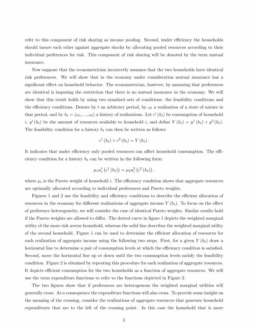
Figures 1 and 2 use the feasibility and efficiency conditions to describe the efficient allocation of

resources in the economy for different realizations of aggregate income Y (ht). To focus on the effect

of preference heterogeneity, we will consider the case of identical Pareto weights. Similar results hold

if the Pareto weights are allowed to differ. The dotted curve in figure 1 depicts the weighted marginal

utility of the more risk averse household, whereas the solid line describes the weighted marginal utility

of the second household. Figure 1 can be used to determine the efficient allocation of resources for

each realization of aggregate income using the following two steps. First, for a given Y (ht) draw a

horizontal line to determine a pair of consumption levels at which the efficiency condition is satisfied.

Second, move the horizontal line up or down until the two consumption levels satisfy the feasibility

condition. Figure 2 is obtained by repeating this procedure for each realization of aggregate resources.

It depicts efficient consumption for the two households as a function of aggregate resources. We will

use the term expenditure functions to refer to the functions depicted in Figure 2.

The two figures show that if preferences are heterogenous the weighted marginal utilities will

generally cross. As a consequence the expenditure functions will also cross. To provide some insight on

the meaning of the crossing, consider the realizations of aggregate resources that generate household

expenditures that are to the left of the crossing point. In this case the household that is more

5

risk averse consumes more than half of aggregate resources. The allocations in this region can be

interpreted as the outcome of the insurance provided by the less risk averse household against adverse

realizations of aggregate resources. Consider now the region to the right of the crossing point. In

this case, the household that is less risk averse consumes more than half of aggregate resources as

a compensation for the insurance provided against adverse aggregate shocks. To summarize, in this

economy the households first eliminate the idiosyncratic uncertainty by pooling their resources and

then insure each other against aggregate shocks by allocating the aggregate resources according to

their preferences for risk.

We will now describe the efficient allocations of resources under the assumption made by the

econometrician that households have identical risk preferences. Figures 3 and 4 depict efficient risk

sharing for the general case of different Pareto weights. They show that the weighted marginal

utilities and hence the household expenditure functions can never cross. The reason for this result is

straightforward. Since it is assumed that the two households have identical risk preferences there is no

scope for mutual insurance. As a consequence, the household with higher Pareto weight will always

consume more than half of aggregate resources. We can therefore conclude that the assumption of

identical preferences for risk is equivalent to the restriction that mutual insurance is an irrelevant

component of efficient risk sharing.

Using this result we can determine how the tests developed in the risk sharing literature perform

when they are used to test efficiency in an economy characterized by heterogeneous risk preferences.

To this end, consider the following generalization of the efficiency test initially proposed by Mace

(1991). Under the assumptions made by the econometrician that the two households in the economy

have identical HARA preferences and share risk efficiently, it is straightforward to show that the

following relationship between household and aggregate consumption must be satisfied:

f(cit+1

)− f(cit

)=

12

2∑

j=1

(f

(cjt+1

)− f

(cjt

)), (1)

where f (c) is a transformation of consumption that varies with the utility function chosen to char-

acterize the household preferences. Specifically, f (c) = c for CARA preferences, f (c) = log (c) for

CRRA preferences, and f (c) = log (a + c) for the general class of HARA preferences. This general-

ization of Mace’s test is useful because the tests used in the papers cited above are a special case of it.

To see this note that under the assumption of CARA preferences, equation (1) establishes that the

first difference in household consumption must equal the first difference in aggregate consumption,

which is the test used in Mace (1991), Townsend (1994), and Ravallion and Chaudhuri (1997). If

preferences are assumed to belong to the CRRA class, according to equation (1) household consump-

tion growth must equal aggregate consumption growth, which is the test used in Cochrane (1991),

Mace (1991), and Altonji, Hayashi, and Kotlikoff (1992).3 Finally if the utility function belongs to3Altug and Miller (1990), Hayashi, Altonji, and Kotlikoff (1996), and in part of their work Attanasio and Davis (1996)

6

the general HARA class, equation (1) still equates household consumption growth with aggregate

consumption growth, but the growth rate must be computed taking into account the subsistence level

a. This is the test used in Ogaki and Zhang (2001).4

Now consider two periods with the following features. In the first period the economy is character-

ized by an adverse realization of aggregate resources, i.e. aggregate resources are on the left of where

the expenditure functions cross. In second period the economy is characterized by a good realization

of aggregate resources, i.e. aggregate resources are on the right of the crossing point. Since the two

households have different preferences for risk, they will insure each other against aggregate shocks.

This implies that between the two periods consumption of the more risk averse household will vary

less than aggregate consumption and consumption of the less risk averse household will vary more.

Formally, the equality tested in previous papers is replaced by the following inequalities:

f(c1t+1

)− f(c1t

)<

12

2∑

j=1

(f

(cjt+1

)− f

(cjt

))< f

(c2t+1

)− f(c2t

).

This implies that, if in the data used by previous papers households have heterogeneous risk prefer-

ences, efficient risk sharing should have been rejected even if households are sharing risk efficiently.5

One additional aspect of the tests used in the past should be discussed before claiming that

heterogeneity in risk preferences may explain previous rejections. In the risk sharing literature the

efficiency condition (1) is tested by adding a variable that captures idiosyncratic shocks to the equation

and by verifying whether the coefficient on this variable is statistically significant. Most of the papers

add changes in household income to equation (1) and they find that the coefficient is statistically

significant and positive. It is important to understand whether heterogeneity in risk preferences can

explain the positive coefficient.

We will show that preference heterogeneity can explain the positive coefficient if less risk averse

households have more volatile income processes. For ease of exposition, we will further simplify the

economy considered in this section by assuming that the only heterogeneity is represented by the

curvature parameter γi, i.e. uic (c) = (a + c)−γi and the Pareto weights are identical. In this economy

the expenditure functions have two main properties. First, they are functions of aggregate resources.

Second, the functions differ across households and the variation is captured by the heterogeneity in

the curvature parameter γi. This implies that the transformation f(c) of the expenditure functions

use preferences that are non-separable between consumption and leisure. The intuition provided in this section appliesalso to those papers. However, a model with nonseparable preferences allows for more general patterns of householdconsumption. We consider this more general case starting from the next section.

4Ogaki and Zhang (2001) apply the test to two different sets of data: the data collected by the International FoodPolicy Research Institute (IFPRI) for Pakistani households and the ICRISAT data for Indian households. When theyuse the test initially introduced by Mace (1991) they do not reject efficiency in Pakistani villages, but they reject thishypothesis for Indian villages. These findings are consistent with the discussion of this section. Homogeneity in riskpreferences can be a good assumption in some environments, but a bad assumption in others.

5The test proposed by Cochrane (1991) is affected by the same problem. The assumption of identical CRRApreferences enables one to include in the constant the terms that capture aggregate quantities, (1 /γj ) log(µt+1 /µt ) inequation (8) in Cochrane (1991). If preferences are heterogeneous the constant will generally be smaller for more riskaverse households and larger for less risk averse households. Therefore the inequality will generally still hold.

7

can be written in the following form:

f i(cit

)= g (Ca

t , γi) .

We can now linearize the transformed expenditure functions by taking a first order Taylor expansion

around the average γi in the economy. We can then compute the first difference of the linearized

functions to obtain the following equation:

∆f i(cit

) ' ∆g (Cat , γ) + (γi − γ)

∂

∂γi∆g (Ca

t , γi)∣∣∣∣γ

. (2)

This equation describes the dynamics of efficient expenditure in an economy with heterogeneity in

risk preferences.

As mentioned above, in previous papers the efficiency test has generally been performed by esti-

mating the following equation:

∆f i(cit

)−∆g (Cat , γ) = α + ξ∆yi

t + εit, (3)

for some function g (.), where yi is income of household i. A comparison of equations (2) and (3)

clarifies the following two points. First, since in the economy households have heterogeneous risk

preferences, there is an omitted variable in equation (3), namely (γi − γ)∂

∂γi∆g (Ca

t , γi)∣∣∣∣γ

. Second,

since the households share risk efficiently, the coefficient ξ on income should be equal to zero. These

two points and standard results on the bias generated by omitted variables imply that the expected

value of the least square estimate of the coefficient on income can be written as follows:

E(ξ)

= V AR(∆yi

t

)−1Cov

(∆yi

t, (γi − γ)∂

∂γi∆g (Ca

t , γi)∣∣∣∣γ

).

Consequently, if the covariance on the right hand side is positive, one should expect ξ to be positive.

The sign of the covariance can be determined by observing that mutual insurance implies that ∆f i(cit

)

is larger for households with risk aversion below the average. From equation (2) it therefore follows

that (γi − γ)∂

∂γi∆g (Ca

t , γi)∣∣∣∣γ

is larger for households with risk aversion below the average. Now

suppose that households that are less risk averse have more volatile income processes. Then it must

be that

Cov

(∆yi

t, (γi − γ)∂

∂γi∆g (Ca

t , γi)∣∣∣∣γ

)> 0,

which implies that the coefficient on individual income will be on average positive. Finally, observe

that one should expect households that are less risk averse to choose income processes with higher

volatility if the following two conditions are fulfilled: households choose their income process before

entering the risk-sharing agreement and the economy is characterized by aggregate shocks.

The discussion in this section indicates that if in the economy under investigation preferences

for risk are heterogeneous the tests used in the past reject efficiency even if households share risk

8

efficiently. It is therefore important to derive a test that enables one to verify whether the null of

homogeneity in risk preferences is rejected in the data. If it is not, one can use the standard tests. If

it is rejected, a test of efficiency is required that allows for differences in risk preferences. The rest of

the paper is devoted to deriving tests that enable one to evaluate the hypotheses of homogeneity in

risk preferences and efficiency.

3 A Model of Efficient Risk Sharing

We use a standard model to characterize efficient risk sharing. In this section we outline its main

features and we derive a new result which is crucial for setting up the homogeneity and efficiency

tests. Consider an economy in which households live for τ periods. For a given history of realizations

ht, in period t household i is endowed with a wage wit (ht) and a total amount of time T i

t (ht) that

can be divided between leisure and labor. The aggregate amount of non-labor resources in the

economy is denoted by Yt (ht), where Yt (ht) may include profits and savings. Let cit (ht) and lit (ht)

be, respectively, consumption and leisure of household i in period t conditional on the history ht.

Household preferences are assumed to be separable over time and across states of nature. They are

allowed to depend on observable and unobservable heterogeneity, which will be denoted by zit (ht)

and ηit (ht). The corresponding utility function ui

[cit (ht) , lit (ht) ; zi

t (ht) , ηit (ht)

]is assumed to be

strictly increasing, strictly concave, and twice continuously differentiable in consumption and leisure.

Households have a common discount factor β and share the same beliefs over histories of realizations,

which are denoted by P (ht).

Efficient risk sharing in this economy can be described using a standard Pareto problem. Let µi be

the Pareto weight assigned to household i with∑n

i µi = 1 and suppose for simplicity that 0 < µi < 1.

The efficient allocation of resources is then the solution of the following problem:

max{ci

t(ht),lit(ht)}

n∑

i=1

µi

τ∑

t=1

βt∑

ht

P (ht) ui[cit (ht) , lit (ht) ; zi

t (ht) , ηit (ht)

](4)

s.t.n∑

i=1

(cit (ht) + wi

t (ht) lit (ht))

= Yt (ht) +n∑

i=1

wit (ht)T i

t (ht) for each t, ht

cit (ht) > 0, 0 ≤ lit (ht) ≤ T i

t (ht) for each t, ht,

where the right hand side of the resource constraint is full income in the economy.

The test of homogeneous risk preferences and the two efficiency tests will be derived using the

expenditure functions discussed in the previous section and depicted in Figures 2 and 4. With non-

separability between consumption and leisure, household expenditure in period t is equal to cit +wi

tlit.

One possible approach that can be used to derive the expenditure functions is to solve the Pareto

problem (4) with respect to consumption and leisure and then substitute the solution in household

expenditure. This approach, however, has one major limitation. The expenditure functions obtained

9

using this method depend on the wages and heterogeneity variables of each household in the economy,

i.e.

ρkt = ci

t + witl

it = ρk

(Yt; w1

t , ..., wnt , z1

t , ..., znt , η1

t , ..., ηnt

)for k = 1, ..., n,

where Y is full income.6 A test based on these expenditure functions is therefore not feasible for

two reasons. First, in every dataset one only observes a fraction of the households that compose the

economy. Some of the variables in the expenditure functions are therefore not observed. Second,

even if all the variables were observed it would generally be infeasible to estimate a function that

depends on so many variables. It is important to remark that the majority of the tests used in the

past are affected by a similar problem. In those tests one has to control for aggregate resources in the

economy, but the researcher only observes the resources of the households in the dataset. We solve

this problem by using a three-stage formulation of the economy which has the same solution as the

standard Pareto program.

We will now describe the three-stage formulation starting from the last stage. Let ρit (ht) be an

arbitrary amount of aggregate resources allocated to household i in period t conditional on the history

ht. In the last stage, conditional on ρit (ht) household i chooses consumption and leisure for period t

and history ht, by solving the following individual problem:

V i(ρi

t (ht) ;wit (ht) , zi

t (ht) , ηit (ht)

)= max

cit(ht),lit(ht)

ui[cit (ht) , lit (ht) ; zi

t (ht) , ηit (ht)

]

s.t. cit (ht) + wi

t (ht) lit (ht) = ρit (ht)

cit (ht) ≥ 0, 0 ≤ lit (ht) ≤ T i

t (ht) .

Consider now the second stage. Let ρi,jt (ht) denote an arbitrary amount of aggregate resources

allocated to the pair composed of households i and j. In the intermediate stage, conditional on

ρi,jt (ht) the pair chooses the optimal amount of resources to allocate to households i and j in period

t and history ht by solving the following problem:7

V i,j(ρi,j

t ; wit, w

jt , z

it, z

jt , η

it, η

jt

)= max

ρit,ρ

jt

µiVi(ρi

t; wit, z

it, η

it

)+ µjV

j(ρj

t ; wjt , z

jt , η

jt

)

s.t. ρit + ρj

t = ρi,jt .

It is worth discussing two features of the second-stage problem. First, since ρkt = ck

t + wkt lkt , its

solution provides the expenditure functions on which the tests will be based. Second, the expenditure

functions obtained using this stage are only function of wages and heterogeneity of households i and

j, i.e.

ρkt = ρk

t

(ρi,j

t , wit, w

jt ; z

it, z

jt , η

it, η

jt

)for k = i, j.

6Note that the assumption that preferences are separable over time and across states enables us to write the expen-diture functions only as a function of variables in period t and history ht.

7Unless required for expositional clarity, the dependence on ht will be suppressed in the rest of the paper.

10

Since in many datasets one observes wages and heterogeneity variables for all pairs of households

in the sample, tests based on expenditure functions are feasible as long as one uses the expenditure

functions obtained in the intermediate stage.

In the first stage full income is optimally allocated to each pair of households. Conditional on

the amount of resources available in the economy in period t and history ht, each pair receives an

allocation that is the solution of the following problem:8

V

(Yt +

n∑

i=1

witT

it ; wt, zt, ηt

)= max{ρ2i−1,2i

t }

n/2∑

i=1

V 2i−1,2i(ρ2i−1,2i

t ; w2i−1t , w2i

t , z2i−1t , z2i

t , η2i−1t , η2i

t

)

s.t.

n/2∑

i=1

ρ2i−1,2it = Yt +

n∑

i=1

witT

it ,

where wt, zt, and ηt are the vectors of wages and heterogeneity variables.

Under the standard assumptions that preferences are separable over time and across states of

nature, it follows that the solution of the three-stage problem is equivalent to the original Pareto

problem, i.e.

τ∑

t=1

βt∑

ht

P (ht) V

(Yt (ht) +

n∑

i=1

wit (ht) T i

t (ht) ; wt (ht) , zt (ht) , ηt (ht)

)=

max{ci

t(ht),lit(ht)}

n∑

i=1

µi

τ∑

t=1

βt∑

ht

P (ht) ui[cit (ht) , lit (ht) ; zi

t (ht) , ηit (ht)

]

s.t.n∑

i=1

(cit (ht) + wi

t (ht) lit (ht))

= Yt (ht) +n∑

i=1

wit (ht)T i

t (ht) for each t, ht

cit (ht) ≥ 0, 0 ≤ lit (ht) ≤ T i

t (ht) for each t, ht.

The intuition for this result is straightforward. Under the assumptions of this paper, the conditions

of the second welfare theorem are fulfilled. As a result the solution of the Pareto problem can be

decentralized using transfers.

4 Testable Implications

In this section we derive the testable implications on which the test of homogeneity in risk preferences

and the efficiency tests are based. They are all derived using the expenditure functions obtained from

the intermediate stage of the efficiency problem described in the previous section. The discussion will

be divided into three parts. In the first part we will consider an economy where households share risk

efficiently and derive a restriction that will enable us to test whether preferences are homogeneous8The Pareto problem can be decomposed in three stages by pairing households in different ways. Here we consider

one possible set of pairs under the assumption that there is an even number of households in the economy. If n is odd,three households will have to be arranged in one group.

11

across households. In the second part we will recover a necessary condition of efficient risk sharing

that can be used to test efficiency even if preferences are heterogeneous. In the last part, we will show

that the necessary condition is also sufficient if no intertemporal variation in real wages is observed

or used.

We will first derive a testable implication for homogeneity in risk preferences. The implication is

based on the following idea. Consider households i and j and suppose that they share risk efficiently.

The discussion in section 2 implies that if their expenditure functions cross, mutual insurance must

be a significant component of efficient risk sharing. If mutual insurance is an important feature of risk

sharing, the two households must have heterogeneous preferences. One can therefore conclude that

under efficiency if the expenditure functions cross the hypothesis of homogeneous risk preferences can

be rejected. This idea is formalized in the following proposition.

Proposition 1 Suppose that household i and j share risk efficiently. If there exist two realizations

of aggregate resources ρi,j and ρi,j such that

ρi(ρi,j , wi, wj ; zi, zj , ηi, ηj

)> ρj

(ρi,j , wi, wj ; zi, zj , ηi, ηj

)

and

ρi(ρi,j , wi, wj ; zi, zj , ηi, ηj

)< ρj

(ρi,j , wi, wj ; zi, zj , ηi, ηj

),

household i and household j cannot have identical preferences.

Proof. In the appendix.

Three remarks are in order. First, Proposition 1 can easily be used to set up a test of preference

homogeneity. For each pair of households in the data one can recover their expenditure functions

and verify whether they cross or not. Second, the preference homogeneity test is valid only under the

maintained assumption that households share risk efficiently. The test is therefore useful only if the

final goal is to test efficiency. Third, if the test does not reject homogeneity in risk preferences one

can test for efficient risk sharing using the standard approach. However, if the hypothesis is rejected

new tests of efficiency are required that allow for heterogeneity in risk preferences.

We will now derive a necessary condition of efficient risk sharing that is satisfied even if households

have different risk preferences. Consider households i and j and observe that under efficiency the

following two restrictions must be fulfilled. First, after controlling for differences across households in

real wages, observable and unobservable heterogeneity, only aggregate resources should affect the ex-

penditure of households i and j. Hence, conditional on wi, wj , zi, zj , ηi, and ηj , for each realization of

ρi,j only one value should be observed for ρi(ρi,j , wi, wj ; zi, zj , ηi, ηj

)and ρj

(ρi,j , wi, wj ; zi, zj , ηi, ηj

).

Second, an increase in aggregate resources should increase expenditure of both households. If one

of these restrictions is not satisfied, household behavior is not only affected by changes in aggregate

12

resources as predicted by efficient risk sharing, but also by idiosyncratic shocks. These two restric-

tions imply that a necessary condition for efficient risk sharing is that ρi(ρi,j , wi, wj ; zi, zj , ηi, ηj

)and

ρj(ρi,j , wi, wj ; zi, zj , ηi, ηj

)must be strictly increasing functions of aggregate resources. The following

proposition formalizes this result.

Proposition 2 Suppose that the utility functions of households i and j are strictly increasing and

concave. Then, if households i and j share risk efficiently, ρi(ρi,j , wi, wj ; zi, zj , ηi, ηj

)and

ρj(ρi,j , wj , wi; zi, zj , ηi, ηj

)are strictly increasing functions of aggregate resources.

Proof. In the appendix.

The result presented in Proposition 2 contains two testable implications. First, after controlling

for aggregate resources, wages, observable and unobservable heterogeneity the expenditure functions

should not depend on other variables that capture idiosyncratic shocks. This testable implication is

a generalization of the standard test of efficiency to an environment with heterogeneous risk pref-

erences. The second testable implication can be described as follows. After controlling for wages,

observable and unobservable heterogeneity, the expenditure functions should be increasing in aggre-

gated resources. To the best of our knowledge this is the first paper to propose this restriction as a

test of efficiency. It has the advantage relative to the first implication that there is no need to use

variables related to idiosyncratic shocks, the choice of which is often arbitrary.

The condition described in Proposition 2 is also sufficient for efficient risk sharing if no intertem-

poral variation in real wages is observed or used to test efficiency. There are two situations in which

this assumption on wages is satisfied. First, only cross-sectional variation in wages is observed or

used by the researcher. Second, household preferences are assumed to be separable between con-

sumption and leisure, which implies that the variation in wages is not exploited in the efficiency tests.

These two situations are the ones considered by the risk sharing literature. Mace (1991), Townsend

(1994), Altonji, Hayashi, and Kotlikoff (1992), Ravallion and Chaudhuri (1997), and Ogaki and Zhang

(2001) assume separability between consumption and leisure. Cochrane (1991) uses a cross-section of

households and hence ignores any longitudinal variation in real wages. Altug and Miller (1990) and

Hayashi, Altonji, and Kotlikoff (1996) exploit longitudinal consumption variation after controlling for

longitudinal variation in leisure. This is equivalent to using longitudinal variation in consumption

after having removed the portion that is explained by longitudinal variation in real wages.

The next proposition formally describes the sufficient condition for efficiency. It shows that if

ρi(ρi,j , wi, wj ; zi, zj , ηi, ηj

)and ρj

(ρi,j , wi, wj ; zi, zj , ηi, ηj

)are strictly increasing functions of ρi,j ,

then it is always possible to find increasing and concave utility functions and Pareto weights such

that efficiency is satisfied.

Proposition 3 Suppose that preferences are separable between consumption and leisure or wi and

wj do not vary. Then, if ρi(ρi,j , wi, wj ; zi, zj , ηi, ηj

)and ρj

(ρi,j , wj , wi; zi, zj , ηi, ηj

)are strictly in-

13

creasing functions of aggregate resources, there exist utility functions that are strictly increasing and

concave such that the two households share risk efficiently.

Proof. In the appendix.

Proposition 3 implies that if only variation in expenditure is used, the only testable implications

of efficient risk sharing are the two implications described in Proposition 2. Any other restriction is

the outcome of the particular functional form selected for household preferences.9

5 Estimation of the Expenditure Functions

The testable implications derived in the previous section can be used to set up tests of homogeneity in

risk preferences and efficiency only if an estimate of the household expenditure functions is available.

In this section we will discuss the method used in this paper in the estimation of these functions.

The estimation approach must allow for heterogeneity in risk preferences. In an environment with

different preferences, there are two features of the expenditure functions that must be considered.

First, households with heterogeneous preferences have expenditure functions with different functional

forms. To address this issue we will estimate the expenditure functions separately for each household.

Second, if risk preferences are heterogeneous there is no close form solution for the expenditure

functions except for the frequently criticized case of CARA utilities. For this reason we will employ

a semi-parametric estimator.

Without data limitations, the expenditure functions can be estimated non-parametrically sep-

arately for each household without making additional assumptions. The dataset employed in this

paper has, however, some limitations that will be discussed in a later section. To overcome them, we

will impose four restrictions on the way observable and unobservable heterogeneity and measurement

errors enter the expenditure functions. First, we will assume that the observable and unobservable

heterogeneity enter the expenditure functions only as a linear combination of the difference between

zi and zj , and ηi and ηj , i.e. only di,j = θi,j

(zi − zj

)+ ηi − ηj affects ρk. This assumption simplifies

significantly the estimation since all the variation in heterogeneity is captured by the single index

di,j . Second, it is assumed that the unobservable component of heterogeneity does not change over

time. Under this assumption, the effect of ηi − ηj can be captured by adding a constant for the pair

of households i and j to the vector of observables z. The constant captures unobservable preference

shocks that are very persistent.10 As a third assumption, we will impose the restriction that the

coefficients on the observable heterogeneity variables are common across households to increase the9Hara (2006) derives a similar result under the assumption that preferences are separable between consumption and

leisure. Our result is more general in the following sense. We show that without separability between consumptionand leisure the condition that expenditure is an increasing function of aggregate resources is sufficient for efficient risksharing only if there is no intertemporal variation in wages.

10The estimator can be modified to accommodate a term ηi − ηj that varies over time. In this case, one can followBlundell and Powell (2001) and consider the expectation of the expenditure functions taken over ηi − ηj .

14

precision of our estimates. Finally, we will allow for measurement errors m in individual expenditure,

which are assumed to be additive and independent of wi, wj , and di,j . Under these assumptions, the

expenditure function of household k can be written as follows:11

ρk = gk(ρi,j , wi, wj , di,j

)+ mk. (5)

Three issues are worth a discussion. First, there is a large class of utilities that generates the

expenditure function described in (5). For instance, all the utility functions that can be written in

the following form:

ui(ci, li, zi, ηi

)= vi

(ci, li

)exp

(θzi + ηi

)

produce expenditure functions consistent with (5). Second, in the model ρi,j is equal to the sum

of individual expenditures. In the estimation, ρi,j will be computed using this relationship. As a

consequence, if the data on individual expenditure are affected by measurement errors, the data on

aggregate resources will also be affected by the same problem. The method used in the estimation must

therefore allow for measurement errors in ρi,j . Third, the assumptions on observable and unobservable

heterogeneity are needed only if one is interested in the economic meaning of z and η and in whether

an economic model can generate the particular functional form imposed on the expenditure functions.

If one is not interested in these issues, observable and unobservable heterogeneity can be introduced

by simply adding a polynomial in z and η to gk(ρi,j

t , wit, w

jt

).

Under the assumptions listed above, the expenditure functions can be estimated using the combi-

nation of two estimators available in the non-parametric literature. The first one is the estimator

developed by Newey et al. (1999). For a given single index di,j it enables us to estimate non-

parametrically the expenditure functions controlling for the endogeneity of ρi,jt . The second one

is the estimator proposed by Ichimura (1993), which will be used to estimate the parameters of the

single index di,j .

We will briefly describe how the two estimators can be employed to recover the expenditure

functions. Suppose first that the parameters defining the heterogeneity term di,j are known. Observe

that the expenditure functions cannot be estimated using standard non-parametric methods because

E[mk|ρi,j

] 6= 0. To address this issue, let q be a set of instruments in the sense that the following

conditions are satisfied:

ρi,j = h(qi,j

)+ ui,j , E

[ui,j |qi,j

]= 0, and E

[mk|ui,j , qi,j

]= E

[mk|ui,j

].

Then, we have that

E[ρk|ρi,j , wi, wj , di,j , qi,j

]= gk

(ρi,j , wi, wj , di,j

)+ E

[mk|ρi,j , wi, wj , di,j , qi,j

]

= gk(ρi,j , wi, wj , di,j

)+ E

[mk|ui,j , qi,j

]= gk

(ρi,j , wi, wj , di,j

)+ λ

(ui,j

),

11The time subscript will be suppressed here and in the remaining sections to simplify the notation.

15

where λ (u) = E[mk|u]

. Newey et al. (1999) propose to estimate the function gk in two steps. In

the first step the error term u is estimated non-parametrically as ui,j = ρi,j − h(qi,j

). In the second

step, the function gk(ρi,j , wi, wj , di,j

)+ λ

(ui,j

)is estimated using the estimated residuals in place of

the true ones. An estimator of the function gk can then be recovered by isolating the components

that do not depend on the residuals u. The estimation will be performed using the series estimator

proposed by Newey et al. (1999) with polynomials.

The parameters of the heterogeneity term di,j are not known, but they can be estimated using

one of the semi-parametric methods developed for the estimation of single-index models. We use the

semi-parametric least square approach proposed by Ichimura (1993).

6 The Tests

In this section we discuss how the tests of preference homogeneity and efficiency can be implemented

using the testable implications derived in section 4. The discussion will be divided into two parts.

In the next three subsections, we will describe how one can derive test statistics for each pair of

households in the data. These test statistics can be used to evaluate preference heterogeneity and

efficiency separately for each observed pair of households. The final goal, however, is to set up tests

that can reject the null hypotheses for the entire group of households. In the last subsection we

discuss how the test statistics computed for each pair can be combined to construct these tests.

6.1 Test of Homogeneous Risk Preferences For a Pair of Households

The test of homogeneity in risk preferences for a pair of households is based on Proposition 1, which

states that under efficiency if two households have identical risk preferences their expenditure functions

should not cross. To simplify the notation we will suppress the dependence of the expenditure

functions on wages, observable and unobservable heterogeneity.

The test can be constructed using the following idea. Consider the pair composed of households i

and j, suppose that they share risk efficiently, and denote by gi,j the difference in their expenditure

functions. Under the null of identical preferences, gi,j as a function of aggregate resources should

always be either positive or negative since there cannot be a crossing. As a consequence, the area

below the positive part of gi,j multiplied by the area below the negative part of gi,j is equal to zero

under the null, but it is positive under the alternative. Formally,

ξi,j1 = −

(∫

{u:gi,j(u)≥0}gi,j (u) du

)(∫

{u:gi,j(u)<0}gi,j (u) du

) {= 0 under H0

> 0 under HA

.

Thus, if ξi,j1 is positive the null hypothesis of homogeneous risk preferences can be rejected.12

12We have also experimented with the simpler test statistic ξi,j = max{gi,j}min{gi,j}. The simulation study that willbe discussed later in the paper suggests, however, that a test based on ξi,j has less power and control than a test basedon ξi,j . The difference in power and control is especially large in the case of measurement errors with high variance.

16

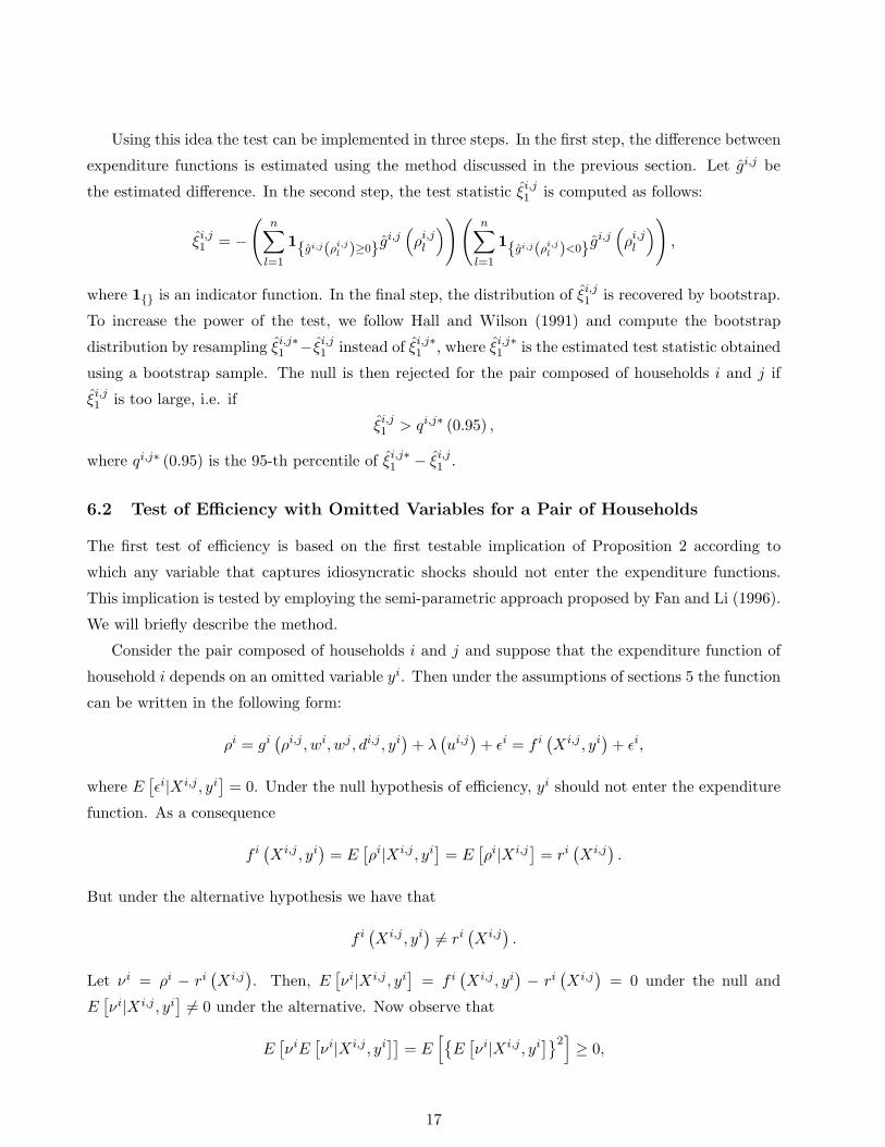
Using this idea the test can be implemented in three steps. In the first step, the difference between

expenditure functions is estimated using the method discussed in the previous section. Let gi,j be

the estimated difference. In the second step, the test statistic ξi,j1 is computed as follows:

ξi,j1 = −

(n∑

l=1

1{gi,j(ρi,jl )≥0}g

i,j(ρi,j

l

))(n∑

l=1

1{gi,j(ρi,jl )<0}g

i,j(ρi,j

l

)),

where 1{} is an indicator function. In the final step, the distribution of ξi,j1 is recovered by bootstrap.

To increase the power of the test, we follow Hall and Wilson (1991) and compute the bootstrap

distribution by resampling ξi,j∗1 −ξi,j

1 instead of ξi,j∗1 , where ξi,j∗

1 is the estimated test statistic obtained

using a bootstrap sample. The null is then rejected for the pair composed of households i and j if

ξi,j1 is too large, i.e. if

ξi,j1 > qi,j∗ (0.95) ,

where qi,j∗ (0.95) is the 95-th percentile of ξi,j∗1 − ξi,j

1 .

6.2 Test of Efficiency with Omitted Variables for a Pair of Households

The first test of efficiency is based on the first testable implication of Proposition 2 according to

which any variable that captures idiosyncratic shocks should not enter the expenditure functions.

This implication is tested by employing the semi-parametric approach proposed by Fan and Li (1996).

We will briefly describe the method.

Consider the pair composed of households i and j and suppose that the expenditure function of

household i depends on an omitted variable yi. Then under the assumptions of sections 5 the function

can be written in the following form:

ρi = gi(ρi,j , wi, wj , di,j , yi

)+ λ

(ui,j

)+ εi = f i

(Xi,j , yi

)+ εi,

where E[εi|Xi,j , yi

]= 0. Under the null hypothesis of efficiency, yi should not enter the expenditure

function. As a consequence

f i(Xi,j , yi

)= E

[ρi|Xi,j , yi

]= E

[ρi|Xi,j

]= ri

(Xi,j

).

But under the alternative hypothesis we have that

f i(Xi,j , yi

) 6= ri(Xi,j

).

Let νi = ρi − ri(Xi,j

). Then, E

[νi|Xi,j , yi

]= f i

(Xi,j , yi

) − ri(Xi,j

)= 0 under the null and

E[νi|Xi,j , yi

] 6= 0 under the alternative. Now observe that

E[νiE

[νi|Xi,j , yi

]]= E

[{E

[νi|Xi,j , yi

]}2]≥ 0,

17

where the inequality follows from the previous discussion and the inequality is replaced by an equality

if and only if the null hypothesis is correct. Fan an Li propose to test for the omitted variable yi

using this inequality and the following idea. If νi and E[νi|Xi,j , yi

]were known, one could estimate

E[νiE

[νi|Xi,j , yi

]]using its sample analog n−1

∑i ν

iE[νi|Xi,j , yi

]. The authors suggest to replace

the residuals νi with estimated ones and E[νi|Xi,j , yi

]with its kernel estimator. Finally, to overcome

the random denominator problem in the kernel estimation, they propose to replace the sample analog

with its density weighted version:

1n

∑

i

[νif

(Xi,j

)]E

[νif

(Xi,j

) |Xi,j , yi]f

(Xi,j , yi

),

where f (.) denotes the probability density function. The test statistic for each household can then

be determined by dividing the estimated sample analog by its estimated standard deviation and by

multiplying it by nhd/2, where n is the number of observations and h is a smoothing parameter in the

kernel estimator. In the present paper we estimate the residuals using the series estimator described

in section 5 and the densities using a standard gaussian kernel estimator.

At this point we have one test statistic for each household in the pair. To compute the test statistic

for the pair observe that efficiency is rejected if yi affects the expenditure function of at least one

household. We can therefore compute the test statistic for the pair ξi,j2 by taking the maximum of

the individual test statistics. Similarly to the homogeneity test, the distribution of the test statistic

for the pair is obtained using bootstrap by resampling ξi,j∗2 − ξi,j

2 . The null hypothesis is then rejected

for the pair composed of households i and j if ξi,j2 is too large, i.e. if

ξi,j2 > qi,j∗ (0.95) .

6.3 Test of Efficiency with Increasing Expenditure Functions For a Pair

The second test of efficient risk sharing is based on the implication that under efficiency the ex-

penditure functions should be increasing in total resources. To implement the test, we employ a

generalization of the monotonicity test introduced by Hall and Heckman (2000) to a model with

multiple regressors and endogeneity.

We will provide the intuition underlying the test using a simpler version of the economy considered

in this paper. Suppose that preferences are separable between consumption and leisure, there is no

observable and unobservable heterogeneity, and no measurement errors. In this case, household i’s

expenditure is only a function of ρi,j and there is no endogeneity issue, i.e.

ρi = g(ρi,j

)+ ε. (6)

Let{(

ρit, ρ

i,jt

), 1 ≤ t ≤ T

}be data generated by equations (6) and denote by

{(ρi

t, ρi,jt

), 1 ≤ t ≤ T

}

the same data sorted in increasing order of aggregate resources ρi,j . Consider a subset of the sorted

18

data{(

ρit, ρ

i,jt

), r ≤ t ≤ s

}and estimate the slope of the linear regression of ρi on ρi,j . Repeat the

last step for any subset of the sorted data that contains enough information to estimate the slope.

Hall and Heckman’s idea is that under the hypothesis that the function g(ρi,j

)is increasing, the

minimum over all the estimated slopes should not be negative.

Formally the test is implemented as follows. For a given integer m that will be defined later, let

r and s be integers that satisfy 0 ≤ r ≤ s − m ≤ T − m and let a and b be scalars. Denote by

h(wi, wj , di,j

)a polynomial in the wages and heterogeneity term, and by δ

(ui

)a polynomial in the

first stage residuals in the estimator proposed by Newey et al. (1999). Define

S (a, b, h, δ|r, s) =s∑

i=r+1

{ρi − [

a + bρi,j + h(wi, wj , di,j

)+ δ

(ui

)]}2.

For each choice of r and s, let a (r, s), b (r, s), h (r, s), and δ (r, s) be the solution of the following least

square problem: (a, b, h, δ

)= argmin S (a, b, h, δ|r, s) .

The variance matrix of the estimated coefficients is equal to σ2 (X ′X)−1, where σ2 is the variance of

the residuals in the expenditure function and X is the matrix of regressors. This implies that the

variance ofb√

(X ′X)−1b,b

is equal to σ2, where (X ′X)−1b,b is the diagonal element of the inverse matrix

that corresponds to b. The test statistic for each household in the pair can then be defined as

ξi3 = max

−

b (r, s)√(X ′X)−1

b,b

: 0 ≤ r ≤ s−m ≤ T −m

.

Note that the integer m plays the role of a smoothing parameter in the sense that larger values of m

reduce the effect of outliers. Similarly to the first efficiency test, the test statistic for the pair ξi,j3 can

be computed by taking the maximum of the two individual test statistics. The test rejects the null if

ξi,j3 is too large.

The distribution of the test statistic is derived using the bootstrap method suggested by Hall and

Heckman (2000). According to this method, the bootstrap distribution should be derived under the

hypothesis that the function under investigation is constant in ρi,j because it is the most difficult

nondecreasing function for which to test. As in the previous tests, the bootstrap distribution is

obtained by resampling ξi,j∗2 − ξi,j

2 . We can then reject the null for the pair composed by households

i and j if

ξi,j3 > qi,j∗ (0.95) .

6.4 Tests at the Economy Level

In this subsection we will explain how the test statistics derived in the previous three subsections

can be combined to obtain one test of preference homogeneity and two tests of efficiency with the

19

following two features. First, each null hypothesis is tested simultaneously for all households in the

economy. Second, if the null is rejected, the tests enable us to determine the fraction of households

for which the hypothesis is rejected.

The tests at the economy level are based on the multiple testing procedure developed in Romano

and Wolf (2005) and Romano, Shaikh, and Wolf (2006).13 Consider n hypotheses H1, ..., Hn and let

T1, ..., Tn be the associated test statistics. Suppose that one is interested in a null hypothesis H0 which

is equal to the intersection of H1, ...,Hn, in the sense that H0 is not rejected only if each individual

hypothesis Hk is not rejected. Romano and Wolf (2005) and Romano, Shaikh, and Wolf (2006)

propose two methods for testing H0. The first method controls the familywise error rate (FWE), i.e.

the probability of rejecting at least one of the true hypotheses. Romano, Shaikh, and Wolf (2006)

provide evidence that if the number of individual hypotheses is large, the method that controls for

the FWE rate is too conservative. They propose an alternative method called k-stepM method which

controls the k-FWE rate, i.e. the probability of rejecting at least k true hypotheses. Since in our

paper the number of individual hypotheses is between 396 and 428, we adopt the k-stepM method.

We will now describe the multiple testing method. Let Tr1 ≥ Tr2 ≥ ... ≥ Trn be the test statis-

tics ordered from the highest to the lowest. For any subset of individual hypotheses D, denote by

k−max {Ti} the k-th largest test statistic and by cD (1− α, k) the 1−α percentile of its sampling dis-

tribution. In the first step, all the individual hypotheses are considered, i.e. D = D1 = {Hr1 , ...,Hrn},and the following generalized confidence region is constructed:

[Tr1 − cD1 ,∞)× ...× [Trn − cD1 ,∞) .

The individual hypothesis Tri is then rejected if 0 6∈ [Tri − cD1 ,∞), or equivalently Tri > cD1 . If in

the first step no individual hypothesis is rejected, the null H0 is also not rejected and the procedure

stops. If at least one hypothesis is rejected H0 is also rejected. If the number of rejections is smaller

than k, the procedure stops. Otherwise, Romano, Shaikh, and Wolf (2006) show that the power is

increased by proceeding to the second step. Let R1 be the number of individual hypotheses rejected

in the first step. In the second step, one considers the individual hypotheses not yet rejected, i.e.

D = D2 ={

HrR1+1 , ..., HrRn

}, and construct the corresponding generalized confidence region:

[TrR1+1 − cD2 ,∞

)× ...× [

TrRn− cD2 ,∞

),

where the threshold cD2 is constructed using the following method. Construct all the possible subsets

that contain the n−R1 hypotheses that were not rejected plus k−1 of the rejected hypotheses. Denote

by D2,i the i-th subset. For each subset compute the 1 − α percentile of the sampling distribution

of the k-th largest test statistic cD2,i (1− α, k). The threshold cD2 is the maximum of all cD2,i . The

13There are other procedures that enable one to test multiple hypotheses. See for instance Holm (1979), Hochbergand Tamhane (1987), and Hommel (1988). The advantage of the methods proposed by Romano and Wolf (2005) andRomano, Shaikh, and Wolf (2006) is that they allow for dependence between the individual hypotheses.

20

hypothesis TrRiis then rejected if TrRi

> cD1 . If the number of rejected hypotheses is smaller than

k one should stop. Otherwise, one continues in this stepwise fashion until less then k hypotheses

are rejected. The 1 − α percentile of the sampling distribution of the k-th largest test statistic is

computed using the bootstrap method illustrated in Romano, Shaikh, and Wolf (2006).

7 The ICRISAT Dataset

The three tests developed in this paper are used to understand risk sharing in rural India using

the Village Level Studies (VLS) started by the ICRISAT. This dataset has been chosen for two

reasons. First, a good understanding of the effect of idiosyncratic and aggregate shocks on household

welfare is particularly important in developing countries, where shocks may have devastating effects

on household resources because of the small number of formal markets. Second, several papers in the

past have tested efficient risk sharing using this dataset. The results obtained here can therefore be

compared with the findings of previous papers.

The ICRISAT started the VLS at six locations in rural India on July 1975. The study added four

villages in 1981. In each village 40 households were selected to represent families in four land holding

classes: 10 from landless laborers; 10 from small farmers; 10 from medium farmers; 10 from large

farmers. The sample used in the estimation is composed of households from only 3 of the 10 villages:

Aurepalle, Shirapur, and Kanzara. We focus our analysis on these three villages for two reasons.

First, data for these villages are available for the entire sample period. Second, previous studies have

only considered these villages. The VLS records data on production, labor supply, assets, price of

goods, rainfall, monetary and non-monetary transaction, household size, age, education, and three

different caste rankings from 1975 to 1985. Townsend (1994) gives a detailed description of the data.

We will therefore discuss only the issues that are specific to our paper.

In the estimation we need data on consumption, labor supply, wages, demographic variables, and

non-labor income. The ICRISAT collects information on these variables approximately every month.

The expenditure functions can therefore be estimated using monthly data. We will now discuss how

these variables are constructed.

Monthly household consumption is calculated using the transaction data from the ICRISAT House-

hold Transaction Schedule. The consumption variable is the sum of consumption on grain, consump-

tion on other food items, namely oil, animal products, fruits and vegetables, and consumption on

other non-durable goods. There are two main problems with using the transaction files: the fre-

quency of the interviews varies; the dates of the interviews differ across households. For example, a

household in Aurepalle was interviewed on January 11, February 10, and March 21 in 1980, whereas

a different household in the same village was interviewed on January 17, February 13, and March

25 in the same year. It is therefore difficult to compare expenditures across households and over

time. To overcome this problem we assume that each interview is characterized by a constant rate of

21

consumption. Under this assumption we can compute monthly consumption using the consumption

data from consecutive interviews. The measure of consumption that we obtain using this method

corresponds to non-durable consumption for the entire household. Since different households have

different size and gender-age structure, we divide household consumption by an age-gender weight

which is constructed following Townsend (1994).14

The construction of the wage and labor supply variables requires a separate discussion. Three

different types of employment and wages are recorded by the ICRISAT. The Labor, Draft Animal,

and Machinery Utilization Schedule contains information on hours, days of employment, and wages

of individuals entering daily employment outside their own farm. In the Household Transaction

Schedule, labor income of individuals with regular jobs outside their own farm is recorded, but there

is no information on the days and hours of employment. We assume that the data on regular labor

income refer to the period covered by the interview and that the individual with the regular job works

8 hours a day for 5 days a week. In the Plot Cultivation Schedule, the ICRISAT records data on

the number of hours supplied by men, women, and children to their own farm and the value of their

labor. The value of own labor is imputed by the ICRISAT on the basis of the village-specific market

wages. The data in these three schedules are collected every interview. We employ this information to

construct the daily wages and labor supply that correspond to each month using the method described

for consumption. Daily labor supply is therefore the average number of hours of employment on daily

jobs, regular jobs, and jobs on own farm supplied by adult members. Daily wages are the average

of total labor income earned on any job by adult members divided by the total number of hours. In

the construction of leisure we follow Rosenzweig (1988) and Townsend (1994) and compute the time

endowment T by assuming that each individual has 26 days per month and 14 hours per day that

can be divided between labor and leisure. The remaining days and hours account for sleep, sickness,

and holidays. The first efficiency test is implemented using non-labor income as the omitted variable.

It is constructed as the sum of income from gifts, dowries, pension, theft, and profits.

The Households Member Schedule records data on demographic variables. We use this information

to construct the vector of observable heterogeneity variables, which is composed of the mean age

of adult household members, the number of infants, the age-gender weight, and the caste ranking

considered in Behrman (1988). Consumption and wages are deflated using the consumer price index

published by the Labour Bureau of India. The set of instruments is constructed using information

on lagged rainfall, lagged total expenditure, and lagged savings.

The sample period is July 1975 to July 1985 for Aurepalle and July 1975 to July 1984 for Shirapur

and Kanzara. We drop the households that leave the sample before 1985 for Aurepalle and 1984 for

Shirapur and Kanzara. This implies that we have up to 126 observations for each household in14The age-gender weight is computed by adding the following numbers: for adult males, 1.0; for adult females, 0.9;

for males aged 13-18, 0.94; for females aged 13-18, 0.83; for children aged 7-12, 0.67; for children aged 4-6, 0.52; forToddlers 1-3, 0.32; and for infants 0.05.

22

Aurepalle and up to 114 observations for each household in Shirapur and Kanzara. In all tests, we

drop a household if it has fewer than 80 data points. Table 1 reports the summary statistics of the

main variables.

8 Simulation Study

In this section we will study the performance of the three tests proposed in this paper using sim-

ulations. The results will enable us to improve the power and control of the tests when they are

implemented using the ICRISAT data. Following Romano, Shaikh, and Wolf (2006) we will focus

on three measures of test performance: the average number of false hypotheses rejected; the average

number of true hypotheses rejected; the empirical FWE rate.

All the simulations share the following features. It is assumed that the group under investigation

is composed of ten households. All households have a utility function which is nonseparable between

consumption and leisure and has the following form:

ui (c, l; z, η) =

(cσi l1−σi + ai

)1−γi

1− γiexp{θz + η}.

This utility generates expenditure functions that satisfy the restrictions discussed in section 5. The

parameters σi and ai are assumed to be identical across households with σi = 0.5 and ai = 1. The

risk aversion parameter γi is allowed to vary across households. Five households are assumed to have

γi = 1.2, whereas the corresponding parameter for the other five households is set to 2.5. Households

can save using a risk-free asset with no constraint on their borrowing ability. The interest rate is fixed

at 0.05 and the discount factor is set equal to 0.95. Each household can draw a high or low daily wage

with equal probability. The high and low wages are set equal to 3 and 5 rupees, respectively. We

allow for unobservable heterogeneity in the form of a pair fixed effect and for observable heterogeneity

using the following four variables: mean adult age, caste ranking, age-gender weight, and number of

infants. Household decisions are simulated for 160 periods. To approximate the length of the panel in

the ICRISAT, the test is then performed using the 120 periods that are between t = 21 and t = 140.

The simulation is repeated 500 times. The distribution of the test statistics is determined using 500

bootstraps.

To evaluate the effect of measurement errors on the outcome of the tests, we add measurement

errors to household expenditure ρi. We consider two types of measurement errors. In the first

case, they are drawn from a normal distribution with mean zero and a negligible standard deviation

(σm = 0.1). In the second case they are drawn from a normal distribution with the same mean

but a standard deviation that is equal to half the standard deviation of the simulated household

expenditure. We expect the two standard deviations used in the simulation to be a lower and upper

bound for the standard deviation of the measurement errors in the data.15 In the homogeneity in risk15Ravallion and Chaudhuri (1997) convincingly argue that there are measurement errors in the ICRISAT. We could

23

preferences test, the effect of measurement errors depends also on the quality of the instruments. In

the simulation of that test we consider two sets of instruments. The first set contains a larger number

of instruments and generates an average R2 for total expenditure of about 0.97, where the average

is computed across pairs. The second set contains fewer instruments and produces an average R2 of

about 0.5.

The implementation of tests requires the researcher to choose k in the k-FWE rate and the order

of the polynomial in ρij . We experimented with several values for k. We report the results for k equal

to 1, 3, and 5, since generally for k greater than 5 the loss in control more than dominates the gain in

power. We also experimented with polynomials of order 1, 2, 3, and 5. For each test, we will report

only the results that are useful to understand the relationship between the order of the polynomial

and the test performance.

To implement the test, one must control for the variation in wages, and in observable and unobserv-

able heterogeneity. We control for this variation in two steps. We first estimate semi-parametrically

the expenditure functions and their differences. We then fix wages and the heterogeneity term at the

household mean and perform the tests.

8.1 Simulations for the Test of Homogeneity in Risk Preferences

In this subsection we evaluate the performance of the test of homogeneity in risk preferences. To that

end, we simulate the decisions of the ten households under the maintained assumption of efficient

risk sharing. The Pareto weights are chosen so that the expenditure functions of households with

heterogenous risk preferences cross. The goal of the simulation study is therefore to evaluate whether

different specifications of the test can detect these crossings. The actual data may correspond to

Pareto weights for which the household expenditure functions do not cross even if preferences are

heterogeneous. The results should therefore be interpreted as an upper bound for the power of the

test.

The results indicate that the performance of the test depends on four features of the simulated

data: the severity of the measurement error problem; the quality of the instruments used to address

it; the order of the polynomial in total expenditure; the choice of k in the k-FWE rate. The results

are reported in table 2. To understand them it is important to remember that the risk aversion

parameter is equal to 1.2 for five households and to 2.5 for the remaining five. In the simulation there

are therefore 25 pairs with heterogeneous preferences and expenditure functions that cross, and 20

pairs with homogeneous risk preferences.

We start the description of the results by discussing the effect of the measurement errors on

the outcome of the test. If the standard deviation of the measurement errors is negligible, the test

can easily detect the existence of heterogeneity in risk preferences. The average rejection of false

not find a paper, however, that estimates their standard deviation.

24

hypotheses is 25 out of 25. If the standard deviation is large the average number of false hypotheses

rejected by the test drops significantly for some specifications of the test. The lowest average is

obtained when we employ the small set of instruments, a polynomial of order 2, and k = 1. For

this specification the average number of correct rejections is just 0.4 out of 25. The number increases

significantly if we use the large set of instruments, a polynomial of order 1, and we set k equal to 5. In

this case the average number of correct rejections is 24.3 out of 25. To understand why measurement

errors have a substantial effect on the power of the test, observe that the test statistic is constructed

using the difference in expenditure functions. In the simulation the difference is generally much smaller

than the actual expenditures. When the measurement errors are drawn from a distribution with a

standard deviation that equals half the standard deviation of household expenditure, the difference in

measurement errors dominates the difference in true expenditures in many instances. It is therefore

difficult for the test to detect a crossing unless a strong set of instruments is used and k is increased.

The measurement errors have very little effect on the number of true hypotheses rejected by the test.

The average number of false rejections is always very small with the highest number being 1 for the

large set of instruments, high σm, k = 5, and a polynomial of order 2.

The order of the polynomial in ρij also has a significant effect on the outcome of the test. The

best performance is obtained when the order is set equal to 1. This result can be explained by noting

that for HARA preferences the efficient expenditure functions are approximately linear in aggregate

expenditure. The difference in expenditure functions is therefore also approximately linear. As a

consequence the standard errors of the estimated difference increase with the order of the polynomial,

which explains the results.

The simulation study also indicates that the choice of k has an important effect on the power of

the test. When the standard deviation of the measurement errors is large the test is too conservative

if k is set equal to 1. When we increase k to 3 or 5 we observe a substantial gain in power with little

loss in control. For instance when we use the large set of instruments and a polynomial of order 1,

an increase in k from 1 to 3 raises the average number of correct rejections from 15.2 to 23.5. At the

same time the average number of false rejections increases only slightly from 0 to 0.4. An additional

increase in k to 5 has only a small effect on the outcome of the test. When we use a polynomial of

order 2 and the small set of instruments k = 5 appears to be the optimal choice.

The test of homogeneity in risk preferences in the ICRISAT will be set up taking into account

the results of the simulation study. In the ICRISAT we expect HARA preferences to be only an

approximation of household preferences. We also expect the standard deviation of the measurement

errors to be between the ones considered in the simulation study. Moreover, the set of instruments

that will be used produces an average R2 of about 0.71. Because of all this, we will implement the

test using two specifications. In the first one we set k equal to 345% of the total number of individual

hypotheses and the order of the polynomial to 1. In the second specification we change the order of

25

the polynomial to 2.

8.2 Simulations for the Efficiency Test with Non-labor Income

In this subsection we will discuss the performance of the efficiency test with non-labor income. Its

evaluation requires the simulation of an economy in which a first group of households share risk

efficiently, whereas efficiency is violated for a second group. We will assume that five households

behave efficiently and that the remaining five are in autarky and can insure themselves against income

shocks only by using the risk-free asset. We therefore have 45 individual hypotheses, 35 of which are

false. It is important to point out that autarky with a risk-free asset is only one possible alternative

to efficiency. Other alternatives are autarky without savings, cooperation without commitment, and

cooperation with asymmetric information. We have chosen autarky with a risk-free asset because it

has been shown in the finance literature that in this environment households can achieve a degree of

insurance similar to the degree that can be achieved in an economy with efficient risk sharing.

The ability of households in autarky to insure themselves against income shocks using the risk-free

asset depends on the properties of the non-labor income process. In the simulation we consider a

process that attempts to replicate non-labor income in the ICRISAT data. It is assumed that the

process is distributed according to a normal distribution with a mean that depends on lagged non-

labor income, mean adult age, caste, number of infants, and age-gender weight. This specification

enables us to capture the fact that non-labor income is highly persistent in the data: everything else

equal, an increase in lagged non-labor income by 100% increases current non-labor income by about

50%. Using this specification and the ICRISAT data we can estimate the mean and variance of the

process. We can then compute the probability of drawing different realizations for non-labor income.

The simulation results for the first efficiency test differ from the results obtained from the homo-

geneity test in two respects. First, in the efficiency test the measurement errors have a smaller effect

on the outcome of the test. To provide the intuition behind this result note that the present test is

based on the estimated expenditure functions and not on their differences. Consequently, measure-

ment errors drawn from the same income process have a smaller effect on the test. For this reason

we report the outcome of the simulation study for only one set of instruments which has an average

R2 slightly lower than 0.9. The second difference is that the best performance is obtained with a

polynomial in ρi,j of order 3. To understand why this test requires a polynomial of higher order,

observe that households that share risk efficiently have expenditure functions that are approximately

linear in total expenditure. A polynomial of order 1 is therefore the optimal choice for this group.

The group of inefficient households, however, have expenditure functions that are non-linear in total

expenditure. As a consequence they require a polynomial of higher order. A polynomial of order

3 enables us to approximate in the best possible way the expenditure functions of both groups of

households. We only report the results for this specification.

26

Table 3 describes the outcome of the simulation study. If the standard deviation of the measure-

ment errors is negligible, the test is able to reject almost all false hypotheses. When k = 1 we reject

on average 34.5 false hypotheses out of 35. When k is set equal to 3 or 5 we reject all false hypotheses.

When we increase the standard deviation, the average number of correct rejections decreases but only

slightly with 28.2 average rejections for k = 1, 34.9 rejections for k = 3, and 35 rejections for k = 5.

The average number of true hypotheses rejected is small for both specifications of the measurement

errors and it is between 0 and 0.56.

The results of the simulation study are used to set up the test that will be used to evaluate

efficiency in Indian villages. The test will be implemented using a polynomial of order 3 in ρij and a

k that corresponds to 345% of total hypotheses.

8.3 Simulations for the Efficiency Test with Increasing Functions

In this section we will describe the performance of the efficiency test with increasing functions. Sim-

ilarly to the non-labor income test, we simulate an economy in which five households share risk

efficiently and five households are in autarky.

The computation of the test statistics for the present test requires a choice for the smoothing

parameter m. We have experimented with different values for m. When the measurement errors have

a negligible standard deviation the power of the test is maximized without sacrificing control when

m is set as low as possible. When the measurement errors have a large standard deviation, however,

we reject too many true hypotheses if m is set too low because the test cannot reduce the impact of

outlying data values. With high standard deviation we obtain the best balance between power and

control when we set m = 15. We report the results for this value of the smoothing parameter.

After having set m = 15, the performance of the test depends on two features of the simulated

data: the choice of k for the k-FWE rate; the order of the polynomial in ρi,j . We report our findings

in table 4 for the two specifications of the measurement errors, for a polynomial in ρij of order 3,

and a polynomial of order 5. The results indicate that the efficiency test with increasing functions

has less power than the test with non-labor income. They also indicate that in this test it is crucial

to increase k to 5 and the order of the polynomial to 5. For this specification, we have the largest

number of correct rejections.

We will now provide the intuition for the lower power of this test. If efficiency is violated the

expenditure functions decrease with aggregate expenditure only if aggregate expenditure is the sum

of a high level of expenditure for one household and a low level of expenditure for the other household.

This event occurs if one household is characterized by a high level of non-labor income, wages, and

savings, whereas non-labor income, wages, and savings are low for the second household. Not all

households experience this type of event in a given simulation. As a consequence the number of false

hypotheses rejected by the test is lower than 35 in some simulations.

27

It is also important to understand why a higher order polynomial increases the power of this

efficiency test. The explanation is related to the bootstrap method used to recover the distribution of

the test statistics. The bootstrap distribution is computed using the approach proposed by Hall and

Heckman (2000). According to it, the bootstrap should be implemented under the assumption that

the function under investigation is constant in ρij . The constant function must be computed using

a non-parametric estimator of the household expenditure functions. Households for which efficiency

is violated have non-linear expenditure functions. If the non-linearities are not properly captured

by the non-parametric estimator, the constant function used in the bootstrap will contain variation

in ρij that will increase the variance of the bootstrap distribution. As a result the number of false

hypotheses rejected drops.

Given the results obtained with the simulations, we will test efficiency with increasing functions

in the ICRISAT by setting the smoothing parameter to 15, the order of the polynomial to 3 and 5,

and k equal to 545% of total individual hypotheses.

9 Results

In this section, we report the outcome of the tests for the three Indian villages considered in this paper.

We will first describe the outcome of the test of homogeneity in risk preferences. The estimation of the

household expenditure functions indicates that every pair of households can be assigned to one of three

different categories: (i) pairs whose expenditure functions do not cross; (ii) pairs with expenditure

functions that cross once; (iii) pairs whose expenditure functions cross twice. Figure 5 depicts one

pair of households for each category. This finding represents a first and informal indication that

heterogeneity in risk preferences is a significant feature of Indian villages. The outcome of the formal

test, which is reported in Table 5, supports this evidence. At the village level, homogeneity in risk

preferences is strongly rejected in all three villages. When we use a polynomial of order 1 in ρi,j we

reject the null in about 25% of possible cases in Aurepalle, in about 16% of possible cases in Shirapur,

and in about 35% of possible cases in Kanzara. When we employ a polynomial of order 2, we obtain

a similar number of rejections in Aurepalle and Shirapur. In Kanzara the number of rejections drops

to about 25% of possible cases. When we perform the test at the caste level, we reject the hypothesis

of identical risk preferences in eight out of thirteen observed castes. These results imply that previous

tests should have rejected efficient risk sharing in Indian villages as long as aggregate shocks have

a significant impact on household behavior and the variable used to capture idiosyncratic shocks is

correlated with risk preferences.

We will now discuss the outcome of the efficiency tests. Before considering the tests proposed

in this paper, we describe the results obtained using the standard test employed by the risk-sharing

literature. The results, which are reported in table 6, are obtained using the specification employed

28

by Townsend (1994). It corresponds to the following efficiency condition:

∆ρit = α0 + α1∆Xt + α2∆ρa

t + α3∆yit,

where ∆ρit, ∆ρa

t , and ∆yit are the first differences in household expenditure, village expenditure, and

household income, and Xt is a vector of control variables that includes wages, mean household age,

caste, number of infants, and age-gender weight. To be able to compare the results of the standard

test with the results of the tests developed in the present paper, expenditure is defined as expenditure

on non-durable consumption plus expenditure on leisure. We reject efficiency in all three villages,

which is consistent with the panel estimates reported in Townsend (1994). The test is also performed

at the caste level for castes that have at least two households in the sample. In this case ∆ρat measures

the first difference in caste expenditure. In Aurepalle we reject the null in two out of six castes, in

Shirapur in two out of three castes, and in Kanzara in two out of four observed castes.

We will now describe the outcome of the two efficiency tests derived in this paper. The results are

reported in Table 7. At the village level, both tests reject efficient risk sharing in all three villages.

Using the non-labor income test, efficiency is rejected for 12 pairs in Aurepalle, 18 pairs in Shirapur,

and 10 pairs in Kanzara. These numbers correspond to about 3% of possible cases in Aurepalle, 5%

of possible cases in Shirapur, and 2% of possible cases in Kanzara.16 The results obtained using the

efficiency test with increasing functions are consistent with the ones obtained using non-labor income.

The only difference worth noting is that with the second test we observe a larger number of rejections

in Kanzara, where the null is violated in about 6% of the cases. The rise in number of rejections is

explained by the increase in k in the k-FWE rate from 3 to 5. When we use k equal to 3, the number

of rejections is always lower for the test with increasing functions. To summarize, at the village level

we observe a small number of rejections, which implies that there is a significant degree of mutual

insurance in Indian villages. But the test can detect a substantial number of rejections even if one

allows for heterogeneity in risk preferences and a general class of utility functions.

Allowing for heterogeneity in risk preferences and a general class of utility functions makes a

significant difference when we test risk-sharing at the caste level. Contrary to the outcome of the

standard test, we find that castes are able to perfectly insure their members. In Aurepalle we cannot

reject efficiency in any of the six observed castes. The same result holds for Shirapur. Kanzara is the

only village in which we observe one caste for which efficiency is rejected. For this caste, the null is

rejected for 1 pair out of 78 possible cases using the non-labor income test and for 5 pairs using the

increasing function test.

One additional point should be discussed. For the caste with ranking 86.25 in Aurepalle and

for the caste with ranking 76.25 in Kanzara we cannot reject the hypothesis of homogeneity in risk16Observe that our tests control the k-FWE rate. This implies that in our tests the probability of rejecting at least

k true hypotheses is controlled to be smaller than or equal to 0.05. The statement that the tests should reject at least5% of total hypotheses is therefore incorrect in this context.

29

preferences, we reject efficiency using the standard test, but we cannot reject efficient risk sharing

using the semi-parametric tests that allow for heterogeneity in risk preferences. In these two cases

the different outcome obtained using our efficiency tests should be attributed to the general class of

utility functions allowed by our tests and not to the presence of heterogeneous risk preferences.

The results presented in this section indicate that it is crucial to allow for heterogeneity in risk

preferences and a general class of preferences if the goal is to understand the risk-sharing institutions

in rural India. The next section attempts to interpret these results using data on transfers and loans.

10 Discussion of Results

Two of the findings reported in the previous section are worth a discussion. First, households that

belong to the same caste are able to perfectly insure each other against risk. Second, efficient risk

sharing is rejected at the village level. The number of rejections is small, which suggests that the

degree of insurance is high. But there is a non-negligible number of cases in which the data indicate

that households that belong to different castes are affected by caste-specific shocks. These two findings

suggest that the relevant social unit in rural India is not the village, as indicated in previous papers,

but the caste. These results are consistent with recent evidence reported in Munshi and Rosenzweig

(2006), where it is shown that to understand mobility in India one should use the caste as the social

unit.17

We will now provide some descriptive evidence about the type or risk-sharing institutions that

castes use to insure their members against different types of shocks. A formal analysis would require

a precise description of each institution, which is beyond the scope of this paper. Using the ICRISAT

data, however, we can give some insight on two institutions that appear to be important as risk-

sharing devices at the caste level: transfers and loans. We use two types of information available in

the ICRISAT. First, the ICRISAT collects data on the amount received by or given to a household

as a transfer or loan. In the ICRISAT questionnaire a transfer is defined as a transaction in which

resources or money change ownership without compensation. A loan is a similar transaction with a

compensation. Second, in the ICRISAT we observe the partner in the transaction, where the list of

partners include caste fellows. We can therefore determine whether a loan or a transfer took place

between two households that belong to the same caste.

Table 8 reports average real per-capita transfers and loans given by and received from households

in the three villages under investigation. There are four patterns that are worth a discussion. First,

transfers are a substantial fraction of non-durable expenditure. In Aurepalle, real per-capita transfers

given and received are on average 14.5% and 13% of non-durable expenditure. In Shirapur, the

transfers given and received are also a high percentage of expenditure at 9.5% and 15%. The village17According to their paper, the correct social unit should be the sub-caste or jati. Our tests of efficiency, however,

cannot reject the hypothesis that the caste is the correct risk-sharing unit.

30

with the lower amount of transfers is Kanzara where transfers given and received are 4.8% and 11.6%.

A second pattern to consider is that the average value of loans received is a large fraction of household

expenditure, whereas the same number for loans given is negligible.

A third feature of the data is that most of the transfers are given to and received from households

that belong to the same caste. In Aurepalle, the transfers given to caste fellows are 83% of total

transfers and the transfers received from caste fellows are 70%. Shirapur and Kanzara are charac-

terized by similar percentages. These findings are different from the results reported by Munshi and

Rosenzweig (2006), where it is suggested that transfers between caste members are negligible. Our

results are more in line with Townsend’s view that transfers are an important source of insurance.

The data on loans given display a similar pattern. In all cases in which we observe some resources

being lent, the loan is given to a caste fellow. When we condition on giving a loan, it is also evident

that the amount of resources transferred to the caste fellow is a large fraction of expenditure. The

data on loans received display a different pattern. Most of the loans are received from households

that do not belong to the same caste.

A last point that should be discussed is that a large fraction of the transfers between caste

fellows is given to and received from households living outside the village boundaries. This pattern is

consistent with previous findings, see for instance Rosenzweig and Stark (1989), which indicate that

the relationship between caste members extends beyond the village.

11 Conclusions

In the paper we show that, if in the data households have heterogeneous risk preferences, the standard

test of efficient risk sharing rejects efficiency even if households share risk perfectly. To address this

problem in the paper we propose a method that enables one to test for efficiency even if risk preferences

are heterogeneous. We apply this method to Indian villages. We find strong evidence against the

common assumption of identical risk preferences. We also find that efficient risk sharing is rejected in

Indian villages, but it is not rejected for the castes that compose those villages. This finding implies

that the only policies that can improve the welfare of individuals living in Indian villages are policies

that insure households against aggregate shocks at the caste, village, or state level.

The method proposed in this paper can be used in other environments provided that a long panel

is available. For instance, the method can be used to test efficient risk sharing across countries

using the long panels that exist at the country level. The method can also be used to test efficient

risk sharing in the US at the country, state, extended-family, or household level using the CEX and

synthetic cohorts.

31

References

Altonji, Joseph G., Fumio Hayashi, and Laurence J. Kotlikoff. 1992. “Is the Extended FamilyAltruistically Linked? Direct Tests Using Micro Data.” The American Economic Review 82 (5):1177–1198 (December).

Altug, Sumru, and Robert A. Miller. 1990. “Household Choices in Equilibrium.” Econometrica 58(3): 543–570 (May).

Attanasio, Orazio, and Steven J. Davis. 1996. “Relative Wage Movements and the Distribution ofConsumption.” The Journal of Political Economy 104 (6): 1227–1262 (December).

Attanasio, Orazio, and Jose Victor Rios-Rull. 2000. “Consumption Smoothing and Extended Fam-ilies.” Manuscript, July.

Behrman, Jere R. 1988. “Intrahousehold Allocation of Nutrients in Rural India: Are Boys Favored?Do Parents Exhibit Inequality Aversion?” Oxford Economic Papers 40 (1): 32–54 (March).

Blundell, Richard, Luigi Pistaferri, and Ian Preston. 2006. “Consumption Inequality and PartialInsurance.” IFS Working Paper.

Blundell, Richard, and James L. Powell. 2001. “Endogeneity in Nonparametric and SemiparametricRegression Models.” Cemmap Working Paper.

Cochrane, John H. 1991. “A Simple Test of Consumption Insurance.” The Journal of PoliticalEconomy 99 (5): 957–976 (October).

Dubois, Pierre. 2004. “Consumption Insurance with Heterogeneous Preferences. Can SharecroppingHelp Complete Markets?” Manuscript, University of Toulouse.

Fan, Yanqin, and Qi Li. 1996. “Consistent Model Specification Tests: Omitted Variables andSemiparametric Functional Forms.” Econometrica 64 (4): 865–890 (July).

Hall, Peter, and Nancy E. Heckman. 2000. “Testing for Monotonicity of a Regression Mean byCalibrating for Linear Functions.” The Annals of Statistics 28 (1): 20–39 (February).

Hara, Chiaci. 2006. “Necessary and Sufficient Conditions for the Efficient Risk-Sharing Rules andthe Representative Consumer’s Utility Function.” Manuscript, Kyoto University.

Hara, Chiaci, James Huang, and Christoph Kuzmics. 2006. “Efficient Risk-Sharing Rules withHeterogeneous Risk Attitudes and Background Risks.” Manuscript, KIER Discussion PaperSeries.

Hayashi, Fumio, Joseph Altonji, and Laurence Kotlikoff. 1996. “Risk-Sharing between and withinFamilies.” Econometrica 64 (2): 261–294 (March).

Heathcote, Jonathan, Kjetil Storesletten, and Gianluca Violante. 2007. “Consumption and LaborSupply with Partial Insurance: An Analytical Framework.” Manuscript.

Hicks, John R. 1990. “Value and Capital.” Oxford: Oxford University Press.

Hochberg, Yosef, and Ajit C. Tamhane. 1987. Multiple Comparisons Procedures. New York: Wiley.

Holm, Sture. 1979. “A Simple Sequentially Rejective Multiple Tests Procedure.” ScandinavianJournal of Statistics 6 (1): 65–70.

32

Hommel, Gerhard. 1988. “A Stagewise Rejective Multiple Test Procedure Based on a ModifiedBonferroni Test.” Biometrika 75 (2): 383–386 (June).

Ichimura, Hidehiko. 1993. “Semiparametric Least Squares (SLS) and Weighted SLS Estimation ofSingle-Index Models.” Journal of Econometrics 58 (1-2): 71–120 (July).

Kocherlakota, Narayana R. 1996. “Implications of Efficient Risk Sharing without Commitment.”Review of Economic Studies 63 (4): 595–609 (October).

Kreps, David M. 1990. A Course in Microeconomic Theory.

Ligon, Ethan. 1998. “Risk Sharing and Information in Village Economies.” Review of EconomicStudies 65 (4): 847–864 (October).

Ligon, Ethan, Jonathan P. Thomas, and Tim Worrall. 2002. “Informal Insurance Arrangementswith Limited Commitment: Theory and Evidence from Village Economies.” Review of EconomicStudies 69 (1): 209–244 (January).

Mace, Barbara J. 1991. “Full Insurance in the Presence of Aggregate Uncertainty.” The Journal ofPolitical Economy 99 (5): 928–956 (October).

Mazzocco, Maurizio. 2004. “Savings, Risk Sharing and Preferences for Risk.” American EconomicReview 94 (4): 1169–1182 (September).

Munshi, Kaivan, and Mark Rosenzweig. 2006. “Why is Mobility in India so Low? Social Insurance,Inequality, and Growth.” CID Working Paper.

Newey, Whitney K., James L. Powell, , and Francis Vella. 1999. “Nonparametric Estimation ofTriangular Simultaneous Equations Models.” Econometrica 67 (3): 565–603 (May).

Ogaki, Masao, and Qiang Zhang. 2001. “Decreasing Relative Risk Aversion and Tests of RiskSharing.” Econometrica 69 (2): 515–526 (March).

Ravallion, Martin, and Shubham Chaudhuri. 1997. “Risk and Insurance in Village India: Comment.”Econometrica 65 (1): 171–184 (January).

Romano, Joseph P., Azeem M. Shaikh, and Michael Wolf. 2006. “Formalized Data Snooping Basedon Generalized Error Rates.” Working Paper, Stanford University.

Romano, Joseph P., and Michael Wolf. 2005. “Stepwise Multiple Testing as Formalized DataSnooping.” Econometrica 73 (4): 1237–1282 (July).

Rosenzweig, Mark R. 1988. “Risk, Implicit Contracts and the Family in Rural Areas of Low-IncomeCountries.” The Economic Journal 98 (393): 1148–1170 (December).

Rosenzweig, Mark R., and Oded Stark. 1989. “Consumption Smoothing, Migration, and Marriage:Evidence from Rural India.” The Journal of Political Economy 97 (4): 905–926 (August).

Schulhofer-Wohl, Sam. 2006. “A Test of Consumption Insurance with Heterogeneous Preferences.”Manuscript, University of Chicago.

Townsend, Robert M. 1994. “Risk and Insurance in Village India.” Econometrica 62 (3): 539–591(May).

33

A Proofs

In all the proofs we will suppress the dependence on observable and unobservable heterogeneity to

simplify the notation.

A.1 Proof of Proposition 1

Proof. This proposition will be proved by contradiction. Suppose household i and j share risk

efficiently and that there exist two income realizations ρi,j and ρi,j such that

ρi(ρi,j ; wi, wj

)> ρj

(ρi,j ; wi, wj

)

and

ρi(ρi,j ; wi, wj

)< ρj

(ρi,j ;wi, wj

).

Assume that household i and j have identical risk preferences. This implies that V i = V j = V , where

V k is the value function of household k introduced in the three-stage formulation of section 3. We

will show that under these conditions efficiency is violated.

Without loss of generality assume that ρi,j < ρi,j . Strict concavity of the household utility func-

tions implies that the corresponding value functions are strictly concave in income.18 Consequently,

Vρ

(ρj

(ρi,j ; wi, wj

))> Vρ

(ρi

(ρi,j ;wi, wj

)).

This implies,

µiVρ

(ρj

(ρi,j ; wi, wj

))> µiVρ

(ρi

(ρi,j ; wi, wj

))= µjVρ

(ρj

(ρi,j ; wi, wj

)),

where the equality follows from efficient risk sharing. Hence, µi > µj .

Now consider the realization ρi,j . Strict concavity of V implies that

Vρ

(ρi

(ρi,j ; wi, wj

))> Vρ

(ρj

(ρi,j ;wi, wj

)). (7)

Consequently,

µiVρ

(ρi

(ρi,j ; wi, wj

))> µiVρ

(ρj

(ρi,j ; wi, wj

))> µjVρ

(ρj

(ρi,j ; wi, wj

)),

where the first inequality follows from (7) and the second one from µi > µj . This implies that

efficiency is not satisfied and hence that the household utility functions cannot be identical.18For a proof see for instance Proposition 3.6 in Kreps (1990).

34

A.2 Proof of Proposition 2

Proof. The proposition will be proved by contradiction. Suppose that households i and j share risk

efficiently and assume that the expenditure function of household i is decreasing in some interval

I = [ρl, ρu]. We will show that efficiency cannot be satisfied.

Consider two realizations of aggregate income ρi,j ∈ I and ρi,j ∈ I with ρi,j > ρi,j . Since the

expenditure function of household i is decreasing in I we have,

ρi(ρi,j ; wi, wj

) ≤ ρi(ρi,j ;wi, wj

).

As a consequence,

µjV jρ

(ρj

(ρi,j ; wi, wj

))= µiV i

ρ

(ρi

(ρi,j ; wi, wj

)) ≥ µiV iρ

(ρi

(ρi,j ; wi, wj

))= µjV j

ρ

(ρj

(ρi,j ; wi, wj

)),

where the two equalities follow from efficiency and the inequality follows from the strict concavity of

V k(ρk

). Hence, by strict concavity of V k

(ρk

), we have

ρj(ρi,j ; wi, wj

) ≤ ρj(ρi,j ;wi, wj

).

This implies that

ρi(ρi,j ;wi, wj

)+ ρj

(ρi,j ; wi, wj

) ≤ ρi(ρi,j ; wi, wj

)+ ρj

(ρi,j ; wi, wj

) ≤ ρi,j < ρi,j ,

which cannot be the efficient allocation of resources since preferences are strictly increasing.

A.3 Proof of Proposition 3

Proof. Suppose that preferences are separable between consumption and leisure or that wi and wj

are constant. Then,

ρi = ρi(ρi,j ;wi, wj

)= ρi

(ρi,j

), (8)

ρj = ρj(ρi,j ;wj , wi

)= ρj

(ρi,j

), (9)

for some functions ρi and ρj .

Under the assumption that ρi and ρj are strictly increasing functions of ρi,j , equations (8) and

(9) can be solved for ρi,j and equated to obtain,

(ρi

)−1 (ρi

)=

(ρj

)−1 (ρj

), (10)

where(ρk

)−1 is the inverse function of ρk. Let g : R+ → R+ be a strictly decreasing function and

µk a scalar satisfying the following conditions: 0 < µk < 1, for k = 1, ...n, where n is the number of

households in the economy;∑n

i=1 µk = 1. Then, equation (10) implies that

µi

g((

ρi)−1 (

ρi))

µi= µj

g((

ρj)−1 (

ρj))

µj. (11)

35

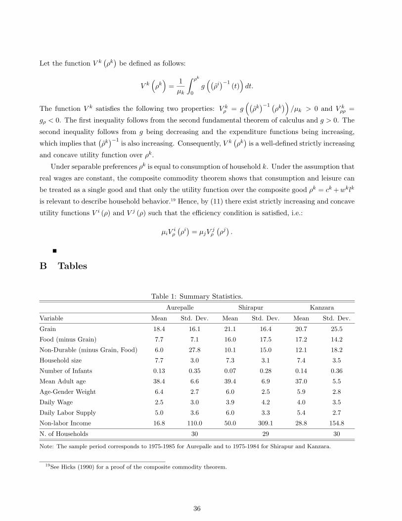
Let the function V k(ρk

)be defined as follows:

V k(ρk

)=

1µk

∫ ρk

0g

((ρi

)−1 (t))

dt.

The function V k satisfies the following two properties: V kρ = g

((ρk

)−1 (ρk

))/µk > 0 and V k

ρρ =

gρ < 0. The first inequality follows from the second fundamental theorem of calculus and g > 0. The

second inequality follows from g being decreasing and the expenditure functions being increasing,

which implies that(ρk

)−1 is also increasing. Consequently, V k(ρk

)is a well-defined strictly increasing

and concave utility function over ρk.

Under separable preferences ρk is equal to consumption of household k. Under the assumption that

real wages are constant, the composite commodity theorem shows that consumption and leisure can

be treated as a single good and that only the utility function over the composite good ρk = ck +wklk

is relevant to describe household behavior.19 Hence, by (11) there exist strictly increasing and concave

utility functions V i (ρ) and V j (ρ) such that the efficiency condition is satisfied, i.e.:

µiViρ

(ρi

)= µjV

jρ

(ρj

).

B Tables

Table 1: Summary Statistics.

Aurepalle Shirapur Kanzara

Variable Mean Std. Dev. Mean Std. Dev. Mean Std. Dev.

Grain 18.4 16.1 21.1 16.4 20.7 25.5

Food (minus Grain) 7.7 7.1 16.0 17.5 17.2 14.2

Non-Durable (minus Grain, Food) 6.0 27.8 10.1 15.0 12.1 18.2

Household size 7.7 3.0 7.3 3.1 7.4 3.5

Number of Infants 0.13 0.35 0.07 0.28 0.14 0.36

Mean Adult age 38.4 6.6 39.4 6.9 37.0 5.5

Age-Gender Weight 6.4 2.7 6.0 2.5 5.9 2.8

Daily Wage 2.5 3.0 3.9 4.2 4.0 3.5

Daily Labor Supply 5.0 3.6 6.0 3.3 5.4 2.7

Non-labor Income 16.8 110.0 50.0 309.1 28.8 154.8

N. of Households 30 29 30

Note: The sample period corresponds to 1975-1985 for Aurepalle and to 1975-1984 for Shirapur and Kanzara.

19See Hicks (1990) for a proof of the composite commodity theorem.

36

Table 2: Simulation Results for the Test of Homogeneity in Risk PreferencesNull Hypothesis Homogeneity in Risk Preferences

Average N. of False Average N. of True Empirical FamilywiseHypotheses Rejected Hypotheses Rejected Error Rate

Order of Polynomial in ρij = 1

Large Instrument Set

σm = 0.01, k=1 25.0/25.0 0.0/20.0 0.0σm = 0.5 ∗ σexp, k=1 15.2/25.0 0.0/20.0 0.0

σm = 0.01, k=3 25.0/25.0 0.1/20.0 0.0σm = 0.5 ∗ σexp, k=3 23.5/25.0 0.4/20.0 0.04

σm = 0.01, k=5 25.0/25.0 0.5/20.0 0.0σm = 0.5 ∗ σexp, k=5 24.3/25.0 0.8/20.0 0.0

Small Instrument Set

σm = 0.01, k=1 25.0/25.0 0.0/20.0 0.0σm = 0.5 ∗ σexp, k=1 3.6/25.0 0.0/20.0 0.0

σm = 0.01, k=3 25.0/25.0 0.1/20.0 0.0σm = 0.5 ∗ σexp, k==3 15.9/25.0 0.2/20.0 0.01

σm = 0.01, k==5 25.0/25.0 0.5/20.0 0.0σm = 0.5 ∗ σexp, k==5 19.2/25.0 0.5/20.0 0.0

Order of Polynomial in ρij = 2

Large Instrument Set

σm = 0.01, k=1 25.0/25.0 0.03/20.0 0.03σm = 0.5 ∗ σexp, k=1 3.6/25.0 0.0/20.0 0.0

σm = 0.01, k=3 25.0/25.0 0.2/20.0 0.0σm = 0.5 ∗ σexp, k=3 15.5/25.0 0.3/20.0 0.02

σm = 0.01, k=5 25.0/25.0 0.6/20.0 0.0σm = 0.5 ∗ σexp, k=5 19.0/25.0 1.0/20.0 0.04

Small Instrument Set

σm = 0.01, k=1 25.0/25.0 0.01/20.0 0.01σm = 0.5 ∗ σexp, k=1 0.4/25.0 0.0/20.0 0.0

σm = 0.01, k=3 25.0/25.0 0.2/20.0 0.0σm = 0.5 ∗ σexp, k==3 5.6/25.0 0.2/20.0 0.01

σm = 0.01, k==5 25.0/25.0 0.7/20.0 0.0σm = 0.5 ∗ σexp, k==5 9.7/25.0 0.8/20.0 0.02

Note: The results are obtained by simulating an economy with ten households that share risk efficiently. Five householdshave a coefficient of risk aversion equal to 1.2 and five households have a coefficient of risk aversion equal to 2.5. Thereare therefore 20 pairs for which the null of identical risk preferences is satisfied and 25 pairs for which the null is violated.

37

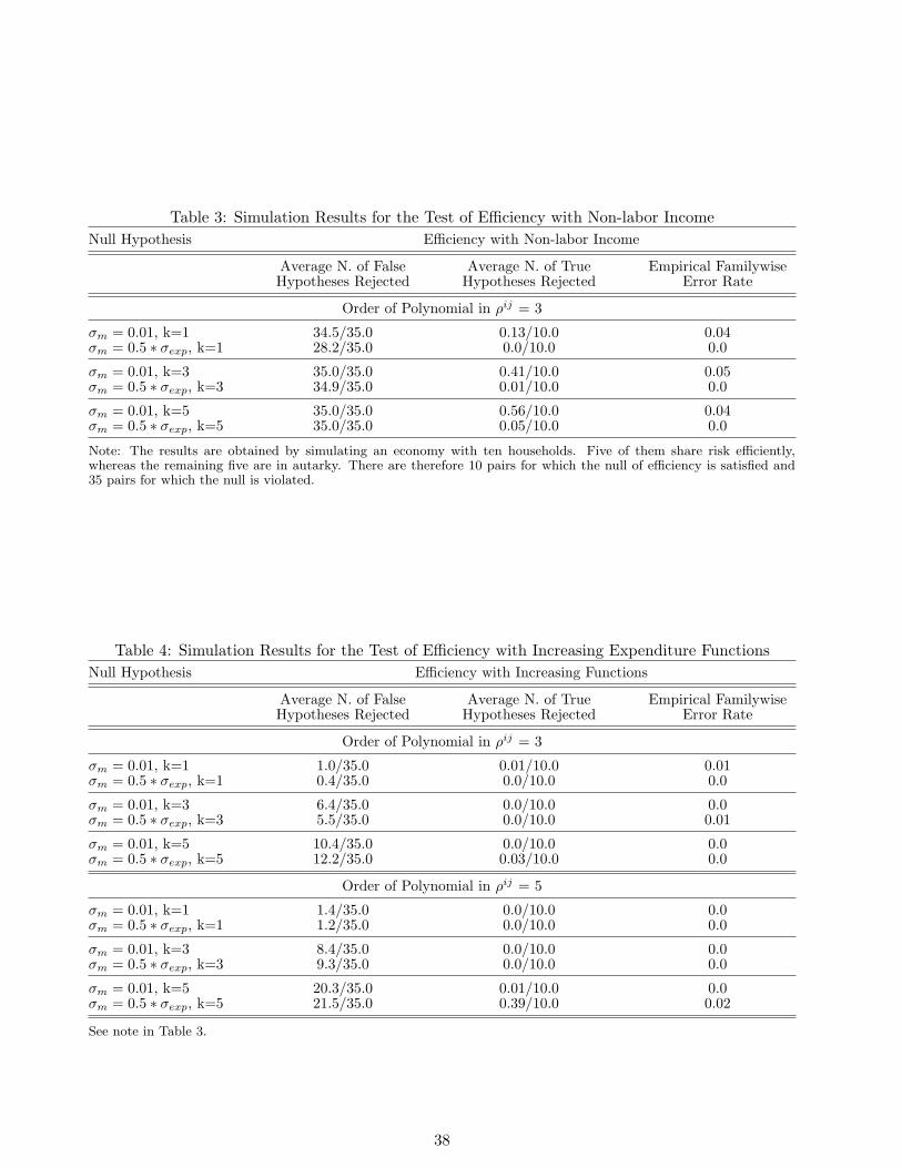
Table 3: Simulation Results for the Test of Efficiency with Non-labor IncomeNull Hypothesis Efficiency with Non-labor Income

Average N. of False Average N. of True Empirical FamilywiseHypotheses Rejected Hypotheses Rejected Error Rate

Order of Polynomial in ρij = 3

σm = 0.01, k=1 34.5/35.0 0.13/10.0 0.04σm = 0.5 ∗ σexp, k=1 28.2/35.0 0.0/10.0 0.0

σm = 0.01, k=3 35.0/35.0 0.41/10.0 0.05σm = 0.5 ∗ σexp, k=3 34.9/35.0 0.01/10.0 0.0

σm = 0.01, k=5 35.0/35.0 0.56/10.0 0.04σm = 0.5 ∗ σexp, k=5 35.0/35.0 0.05/10.0 0.0

Note: The results are obtained by simulating an economy with ten households. Five of them share risk efficiently,whereas the remaining five are in autarky. There are therefore 10 pairs for which the null of efficiency is satisfied and35 pairs for which the null is violated.

Table 4: Simulation Results for the Test of Efficiency with Increasing Expenditure FunctionsNull Hypothesis Efficiency with Increasing Functions

Average N. of False Average N. of True Empirical FamilywiseHypotheses Rejected Hypotheses Rejected Error Rate

Order of Polynomial in ρij = 3

σm = 0.01, k=1 1.0/35.0 0.01/10.0 0.01σm = 0.5 ∗ σexp, k=1 0.4/35.0 0.0/10.0 0.0

σm = 0.01, k=3 6.4/35.0 0.0/10.0 0.0σm = 0.5 ∗ σexp, k=3 5.5/35.0 0.0/10.0 0.01

σm = 0.01, k=5 10.4/35.0 0.0/10.0 0.0σm = 0.5 ∗ σexp, k=5 12.2/35.0 0.03/10.0 0.0

Order of Polynomial in ρij = 5

σm = 0.01, k=1 1.4/35.0 0.0/10.0 0.0σm = 0.5 ∗ σexp, k=1 1.2/35.0 0.0/10.0 0.0

σm = 0.01, k=3 8.4/35.0 0.0/10.0 0.0σm = 0.5 ∗ σexp, k=3 9.3/35.0 0.0/10.0 0.0

σm = 0.01, k=5 20.3/35.0 0.01/10.0 0.0σm = 0.5 ∗ σexp, k=5 21.5/35.0 0.39/10.0 0.02

See note in Table 3.

38

Table 5: Test Of Homogeneity In Risk Preferences.N. of Hypotheses/Pairs N. of Rejections N. of Rejections

1st Order Polyn. in ρij 2nd Order Polyn. in ρij

Aurepalle

All Households 424 104/424 113/424

By caste

Caste Score=7.5 10 2/10 0/10

Caste Score=18.75 1 0/1 0/1

Caste Score=30 10 0/10 0/10

Caste Score=55 26 0/26 4/26

Caste Score=86.25 10 0/10 0/10

Caste Score=97.5 1 0/1 1/1

Shirapur

All Households 396 62/396 69/396

By caste

Caste Score=5 6 0/6 1/6

Caste Score=23.75 26 1/26 1/26

Caste Score=72.5 78 7/78 6/78

Kanzara

All Households 428 148/428 107/428

By caste

Caste Score=11.25 8 0/8 0/8

Caste Score=55 78 11/78 8/78

Caste Score=76.25 1 0/1 0/1

Caste Score=91.25 6 2/6 1/6

Note: The sample period corresponds to 1975-1985 for Aurepalle and to 1975-1984 for Shirapur and Kanzara. Theresults are obtained using a k in the k-FWE rate that corresponds to 3/45% of total hypotheses. The significance levelis 0.05. Household expenditure is the sum of expenditure on non-durable consumption and expenditure on leisure. Thecaste ranking corresponds to the one considered in Behrman (1988).

39

Table 6: Standard Test of Efficient Risk Sharing

Coefficient on Non-labor Income Standard Error N. Observations

Aurepalle

All Households 0.014∗∗ 0.005 2822

By caste

Caste Score=7.5 0.075 0.062 582

Caste Score=18.75 0.032 0.032 217

Caste Score=30 0.038 0.030 493

Caste Score=55 0.038∗∗ 0.019 763

Caste Score=86.25 0.012∗ 0.007 541

Caste Score=97.5 −0.004 0.011 170

Shirapur

All Households 0.011∗∗ 0.003 2537

By caste

Caste Score=5 −0.019 0.034 378

Caste Score=23.75 0.012∗∗ 0.005 733

Caste Score=72.5 0.011∗∗ 0.004 1426

Kanzara

All Households 0.020∗∗ 0.004 2565

Caste Score=11.25 0.009 0. 017 558

Caste Score=55 0.023∗∗ 0.010 1240

Caste Score=76.25 0.030∗∗ 0.008 258

Caste Score=91.25 0.002 0.007 479

See note in Table 5. (**) and (*) indicate that the coefficient is significant, respectively, at the 5 and 10 percent level.

40

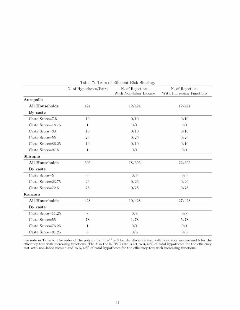
Table 7: Tests of Efficient Risk-Sharing.N. of Hypotheses/Pairs N. of Rejections N. of Rejections

With Non-labor Income With Increasing Functions

Aurepalle

All Households 424 12/424 12/424

By caste

Caste Score=7.5 10 0/10 0/10

Caste Score=18.75 1 0/1 0/1

Caste Score=30 10 0/10 0/10

Caste Score=55 26 0/26 0/26

Caste Score=86.25 10 0/10 0/10

Caste Score=97.5 1 0/1 0/1

Shirapur

All Households 396 18/396 22/396

By caste

Caste Score=5 6 0/6 0/6

Caste Score=23.75 26 0/26 0/26

Caste Score=72.5 78 0/78 0/78

Kanzara

All Households 428 10/428 27/428

By caste

Caste Score=11.25 8 0/8 0/8

Caste Score=55 78 1/78 5/78

Caste Score=76.25 1 0/1 0/1

Caste Score=91.25 6 0/6 0/6

See note in Table 5. The order of the polynomial in ρi,j is 3 for the efficiency test with non-labor income and 5 for theefficiency test with increasing functions. The k in the k-FWE rate is set to 3/45% of total hypotheses for the efficiencytest with non-labor income and to 5/45% of total hypotheses for the efficiency test with increasing functions.

41

Table 8: Average Real Per-capita Transfers and Loans in Rural Villages.

Aurepalle Shirapur Kanzara

Variable Mean % of Expen. Mean % of Expen. Mean % of Expen.

Real Per-capita Non-durable Expen. 33.1 − 47.3 − 50.0 −Real Per-capita Transfers Given

Total Transfers 4.8 14.5% 4.5 9.5% 2.4 4.8%

Total Transfers within Village 2.3 7.0% 1.5 3.2% 1.5 3%

Tr. to Relatives/Caste Fellows 4.0 12.1% 3.9 8.3% 2.1 4.2%

Tr. to Relat./Caste Fellows w. Village 2.2 6.7% 1.1 2.3% 1.4 2.8%

Real Per-capita Transfers Received

Total Transfers 4.3 13.0% 7.1 15% 5.8 11.6%

Total Transfers within Village 1.2 3.6% 1.9 4% 4.7 9.4%

Tr. to Relatives/Caste Fellows 3.0 9.1% 5.5 11.6% 3.3 6.6%

Tr. to Relat./Caste Fellows w. Village 0.5 1.5% 0.9 1.9% 3.2 6.4%

Real Per-capita Loans

Loans Given 0.0 0% 0.30 0.6% 0.04 0.1%

Loans Given to Relatives/Caste Fellows 0.0 0% 0.30 0.6% 0.04 0.1%

Loans Received 13.9 42.0% 20.0 42.0% 8.3 17.0%

Loans received from Relat./Caste Fellows 0.29 0.9% 0.74 1.6% 0.19 0.4%

Real Per-capita Loans Conditional on a Positive Amount

Loans Given 0.0 – 42.0 – 20.7 –

Loans given to Relatives/Caste Fellows 0.0 – 42.0 – 20.7 –

Loans Received 38.2 – 57.8 – 45.4 –

Loans received from Relat./Caste Fellows 0.8 – 2.1 – 1.0 –

Exchanged Laborers and Bullocks

Exchanged Laborers 0.1 0.3% 0.2 0.4% 0.1 0.2%

Exchanged Bullocks 0.32 1% 0.9 1.9% 0.4 0.8%

Note: In the ICRISAT questionnaire, a transfer is defined as a transaction in which resources or money change ownershipwithout compensation. A loan is a similar transaction with a compensation.

42

F Figures

Figure 1: Efficiency Condition with Heterogeneous HARA Preferences and µ1 = µ2.

MU of HH 1: a=–2.0,gamma1=2.50MU of HH 2: a=–2.0,gamma2=1.25

Risk Sharing

0.6

0.8

1

1.2

1.4

MU

2.8 2.9 3 3.1 3.2 3.3 3.4Household Consumption

Figure 2: Efficient Consumption with Heterogeneous HARA Preferences and µ1 = µ2.

Cons. of HH 1: a=–2,gamma1=2.50Cons. of HH 2: a=–2,gamma2=1.25

Risk Sharing

2.4

2.6

2.8

3

3.2

3.4

3.6

C

5 5.2 5.4 5.6 5.8 6 6.2 6.4 6.6 6.8 7Aggregate Resources

43

Figure 3: Efficiency Condition with Identical HARA Preferences and µ1 > µ2.

MU of HH 1: a=–2.0,gamma1=1.25MU of HH 2: a=–2.0,gamma2=1.25

Risk Sharing

0.2

0.4

0.6

0.8

1

MU

3 3.5 4 4.5 5 5.5 6Household Consumption

Figure 4: Efficient Consumption with Identical HARA Preferences and µ1 > µ2.

Cons. of HH 1: a=–2,gamma1=1.25Cons. of HH 2: a=–2,gamma2=1.25

Risk Sharing

2.4

2.6

2.8

3

3.2

3.4

3.6

3.8

C

5 5.2 5.4 5.6 5.8 6 6.2 6.4 6.6 6.8 7Aggregate Resources

44

Figure 5: Expenditures as a Function of Aggregate Resources.

050

100

150

200

Expe

nditu

re F

unct

ions

50 100 150 200 250 300Aggregate Resources

HH 1’s estimated expend. fn. HH 2’s estimated expend. fn.

050

100

150

200

250

Expe

nditu

re F

unct

ions

0 100 200 300 400Aggregate Resources

HH 1’s estimated expend. fn. HH 2’s estimated expend. fn.

050

100

150

200

250

Expe

nditu

re F

unct

ions

0 100 200 300 400Aggregate Resources

HH 1’s estimated expend. fn. HH 2’s estimated expend. fn.

45