Testing a Resolution-Independent Parameterization of Deep

Testing a Resolution-Independent Parameterization of Deep Convection

David Randall, Minoru Chikira, Donald Dazlich, and Shrinivas Moorthi

Testing a Resolution-Independent Parameterization of Deep Convection

David Randall, Minoru Chikira, Donald Dazlich, and Shrinivas Moorthi

Work carried out for a Climate Process Team led by Steve Krueger.

The nature of a model’s subgrid-scale physical processes depends on the horizontal grid spacing.

Parameterizations for low-resolution models describe the collective effects of many clouds, including strong convective transports.

Parameterizations for high-resolution models describe what happens inside individual clouds.

Low resolution High resolution

An example of resolution-dependence

Jung, J.-H. and A. Arakawa, 2004.: The resolution dependency of model physics: Illustrations from nonhydrostatic model experiments. J. Atmos. Sci., 61, 88-102.

4

atmospheric modeling is quite different from such a case because the spectrum is virtually

continuous due to the existence of mesoscale phenomena.

Fig. 2. Domain- and ensemble-averaged profiles of the "required source" for (a) moist static energy (divided by cp ) and (b) total airborne water mixing ratio (multiplied by L / cp ) due to cloud microphysics under strong large-scale forcing over land obtained with different horizontal grid sizes and different time intervals of implementing physics. The two extreme profiles shown in red and green approximately represent the true and apparent sources, respectively. Redrawn from Jung and Arakawa (2004). Jung and Arakawa (2004) showed convincing evidence for the transition of model physics

as the resolution changes by performing budget analysis of data simulated by a CRM with

different space/time resolutions. By comparing the results of low-resolution test runs without

cloud microphysics over a selected time interval with those of a high-resolution run with

cloud microphysics (CONTROL), they identified the apparent microphysical source

“required” for the low-resolution solution to be equal to the space/time averages of the high-

resolution solution. This procedure is repeated over many realizations selected from

CONTROL. Figure 2(a) shows examples of the domain- and ensemble-averaged profiles of

the required source of moist static energy obtained in this way. Here moist static energy is

defined by cpT + Lqv + gz , where T and qv are temperature and water vapor mixing ratio,

respectively, cp is the specific heat at constant pressure, L is the latent heat per unit , and

gz is geopotential energy. The profiles shown in red and green are obtained using (2km, 10

qv

Required Moist Static Energy Source

Resolution-independent cumulus parameterizations

Updrafts occupya small fraction of each grid cell.

Low resolution

Convective transport on subgrid scale

Quasi-equilibrium



Low resolution


Quasi-equilibrium

Some grid cells are almost filled by updrafts.

High resolution

Convective transport on grid scale

Non-equilibrium



Low resolution


A resolution-independent cumulus parameterization must determine , the fraction of each grid cell that is occupied by convective updrafts.

σ

Quasi-equilibrium

Some grid cells are almost filled by updrafts.

High resolution

Convective transport on grid scale

Non-equilibrium

• Individual clouds when/where the resolution is high.

• Parameterized convection when/where resolution is low.

• Continuous scaling.

•One set of equations, one code.

• Physically based.

The Unified Parameterizationof Arakawa and Wu

Goals:

Atmos. Chem. Phys., 14, 5233–5250, 2014www.atmos-chem-phys.net/14/5233/2014/doi:10.5194/acp-14-5233-2014© Author(s) 2014. CC Attribution 3.0 License.

A scale and aerosol aware stochastic convective parameterization forweather and air quality modelingG. A. Grell1 and S. R. Freitas21Earth Systems Research Laboratory of the National Oceanic and Atmospheric Administration (NOAA), Boulder,Colorado 80305-3337, USA2Center for Weather Forecasting and Climate Studies, INPE, Cachoeira Paulista, Sao Paulo, Brazil

Correspondence to: G. A. Grell ([email protected])

Received: 27 July 2013 – Published in Atmos. Chem. Phys. Discuss.: 11 September 2013Revised: 30 January 2014 – Accepted: 25 March 2014 – Published: 27 May 2014

Abstract. A convective parameterization is described andevaluated that may be used in high resolution non-hydrostaticmesoscale models as well as in modeling system with un-structured varying grid resolutions and for convection awaresimulations. This scheme is based on a stochastic approachoriginally implemented by Grell and Devenyi (2002). Twoapproaches are tested on resolutions ranging from 20 kmto 5 km. One approach is based on spreading subsidenceto neighboring grid points, the other one on a recently in-troduced method by Arakawa et al. (2011). Results frommodel intercomparisons, as well as verification with obser-vations indicate that both the spreading of the subsidenceand Arakawa’s approach work well for the highest resolu-tion runs. Because of its simplicity and its capability for anautomatic smooth transition as the resolution is increased,Arakawa’s approach may be preferred. Additionally, inter-actions with aerosols have been implemented through acloud condensation nuclei (CCN) dependent autoconversionof cloud water to rain as well as an aerosol dependent evap-oration of cloud drops. Initial tests with this newly imple-mented aerosol approach show plausible results with a de-crease in predicted precipitation in some areas, caused by thechanged autoconversion mechanism. This change also causesa significant increase of cloud water and ice detrainment nearthe cloud tops. Some areas also experience an increase of pre-cipitation, most likely caused by strengthened downdrafts.

1 Introduction

There are many different parameterizations for deep andshallow convection that exploit the current understandingof the complicated physics and dynamics of convectiveclouds to express the interaction between the larger scaleflow and the convective clouds in simple “parameterized"terms. These parameterizations often differ fundamentallyin closure assumptions and parameters used to solve theinteraction problem, leading to a large spread and uncer-tainty in possible solutions. For some interesting reviewarticles on convective parameterizations the reader is re-ferred to Frank (1984), Grell (1991), Emanuel and Raymond(1992), Emanuel (1994), and Arakawa (2004). New ideasthat have recently been implemented include built-in stochas-ticism (Grell and Devenyi, 2002; Lin and Neelin, 2003),the super parameterization approach (Grabowski and Smo-larkiewicz, 1999; Randall et al., 2003), and a lattice typestochastic multi-cloud model for convective parameteriza-tions (Khouider 2014).An additional complication that is gaining attention

rapidly is the use of convective parameterizations on socalled “gray scales” (Kuell et al., 2007; Mironov, 2009; Ger-ard et al., 2009; Yano et al., 2010). With the increase in com-puter power, high resolution numerical modeling using hor-izontal grid scales of dx < 10 km is becoming widespread,even at operational centers. On these types of resolutions,many of the assumptions that are made in deriving the theorybehind convective parameterizations are no longer valid. Onthe other hand, to properly resolve convection, the horizontalresolutions of these gray scales are also inadequate (see also

Published by Copernicus Publications on behalf of the European Geosciences Union.

The Unified Parameterizationis a “framework.”

The Unified Parameterization is built on top of a user-supplied conventional parameterization.

The conventional parameterization has to determine the updraft vertical velocity.

At low resolution, the conventional parameterization dominates.

Two ways to close a parameterization

Mc ≡ ρσ wc −w( )Closures typically determine the convective mass flux:

.


Mc ≡ ρσ wc −w( )If the updraft vertical velocity is also known, then sigma can be computed by division. With this approach, however, there is no guarantee that

σ ≤1 .

Closures typically determine the convective mass flux:

.


Mc ≡ ρσ wc −w( )

Alternatively, we can formulate a closure for sigma itself, and design the closure so that sigma cannot be larger than one.

In that case, if the updraft vertical velocity is known, then the convective mass flux can be computed by multiplication.

If the updraft vertical velocity is also known, then sigma can be computed by division. With this approach, however, there is no guarantee that

σ ≤1 .

Closures typically determine the convective mass flux:

.

What does sigma closure mean?

We can interpret sigma as the fractional area covered by one updraft, multiplied by the number of updrafts.

Closing for sigma is like closing for the number of updrafts.

The conventional parameterization

The conventional parameterization uses a conventional closure, such as quasi-equilibrium, and is based on the usual assumption of small sigma.

Mc( )E = ρσ wc −w( )

The mass flux given by the conventional parameterization is defined by

.

How do we close for sigma?

σ =Mc( )E

ρ wc −w( )assuming small sigma

For the conventional parameterization

.


σ =Mc( )E



σ =Mc( )E

ρ wc −w( )+ Mc( )E

Close the Unified Parameterization by modifying the above formula to

.

.


σ =Mc( )E



This gives small sigma and is consistent with the conventional parameterization when .Mc( )E ≪ ρ wc −w( )

It gives when .σ →1 Mc( )E ≫ ρ wc −w( )

σ =Mc( )E

ρ wc −w( )+ Mc( )E


.

.


σ =Mc( )E


It is similar but not identical to the closure proposed by Arakawa & Wu.


This gives small sigma and is consistent with the conventional parameterization when .Mc( )E ≪ ρ wc −w( )

It gives when .σ →1 Mc( )E ≫ ρ wc −w( )

σ =Mc( )E

ρ wc −w( )+ Mc( )E


.

.

What makes sigma go to one?

When the grid-scale motion is strongly upward, which can happen with high resolution, a conventional parameterization has to fight hard to stabilize the column.

This causes the mass flux determined by the conventional closure to become very large:

Mc( )E ≫ ρ wc −w( ) .

What makes sigma go to one?

When the grid-scale motion is strongly upward, which can happen with high resolution, a conventional parameterization has to fight hard to stabilize the column.

This causes the mass flux determined by the conventional closure to become very large:

Mc( )E ≫ ρ wc −w( )

This will never happen with low resolution unless the model is blowing up!

.

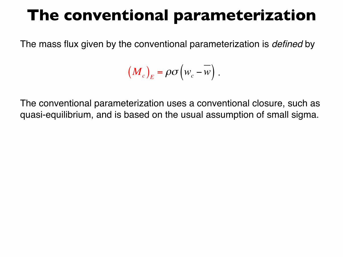
For , the parameterized fluxes become small.

Mc = 1−σ( ) Mc( )E

Combining this with our closure,

The parameterized mass flux goes to zero as sigma goes to one.

Mc = ρσ wc −w( )

For the unified parameterization,

σ =Mc( )E

ρ wc −w( )+ Mc( )E

we find that

σ →1

,

.

.

Use a CRM to test ideas.

8

becomes the gird-scale circulation. The cumulus parameterization should play no role in this

limit. More generally, it is important to remember that parameterizations are supposed to

formulate only the subgrid effects of cumulus convection, NOT its total effects involving gird-

scale motion. Otherwise the parameterization may overdo its job, over-stabilizing the grid-

scale fluctuations that are supposed to be explicitly simulated.

To visualize the problem to be addressed, we have performed two numerical simulations

using a CRM, one with and the other without background shear. The model used for these

simulations is the 3-D vorticity equation model of Jung and Arakawa (2008) applied to an

idealized horizontally-periodic domain. The horizontal domain size and the horizontal grid

size are 512 km and 2km, respectively. Other experimental settings follow the benchmark

simulations performed by Jung and Arakawa (2010).

Figure 4 shows snapshots of the vertical velocity w at 3 km height simulated (a) with and

(b) without background shear. As we can see from these snapshots, these two runs represent

quite different cloud regimes. To see the grid-size dependence of the statistics, we divide the

original CRM domain (512 km) into sub-domains of same size to repcresent the GCM grid

cells.

Fig. 4 Snapshots of the vertical velocity w at 3 km height simulated (a) with and (b) without background shear, and examples of sub-domains used to see the grid-size dependence of the statistics.

Vertical velocity 3 km above the surface Subdomain size,used to analyze dependence on grid spacing

Figure from Akio Arakawa

SGS flux as a function of grid size

10

domains (not shown). This transport may be written as < wh > , where the overbar denotes

the average over all CRM grid points in the sub-domain and, as defined earlier, < > is the

ensemble average over all sub-domains with σ > 0 . To distinguish this transport from the

eddy transport, we call this transport the “total transport” of h. The red lines in Fig. 6 show the

diagnosed total transport, again at z = 3km , for each sub-domain size d. This transport

rapidly increases as d decreases for both the (a) shear and (b) non-shear cases, showing that

active updrafts are better reoresented with higher resolutions. The green lines in the figure, on

the other hand, show the ensemble-average eddy transport given by < ′w ′h > , where

′w ≡ w −w and ′h ≡ h − h . For large sub-domain sizes, say for d ≥ 32 km , the total transport

is almost entirely due to the eddy transport < ′w ′h > . With smaller sub-domain sizes,

however, < ′w ′h > is only a fraction of < wh > and vanishes for d = 2 km. Recall that, as

indicated in the figure, what needs to be parameterized is the eddy transport, not the total

transport, and the difference between the total and eddy transports must be explicitly

simulated. We note that the contribution from the eddy transport is larger for the non-shear

case although there is no significant qualitative difference between the two cases in the way

the transports depend on the resolution.

Fig. 6 The diagnosed total transport and eddy transport of moist static energy divided by c p at z = 3 km for each sub-domain size d.

< wh >

Red curve is total flux.Green curve is subgrid flux to be parameterized.

The subgrid part is dominant at low resolution, but negligible at high resolution.


Flux partitioning

Numbers and colors show percentage of the total flux due to unresolved processes.

!

kind of transport should also exist to some extent forsmaller values of s . [Here the ‘‘internal structure’’ refersto those still resolved by the CRM, not subcloud eddiessuch as those discussed by Emanuel (1991)].Figure 8 is the same as Fig. 7, but for cpT, Lqy, and

Lql, where ql is the mixing ratio of liquid water. FromFigs. 8a and 8b, we see that the vertical transport of moiststatic energy is dominated by that of water vapor. FromFigs. 8b and 8c, on the other hand, the transports of watervapor and liquid water are almost equally responsiblefor the vertical transport of total (airborne) water. Thes dependence of the partition between the eddy- andgrid-scale transports of these variables is quite similarto that for moist static energy shown in Fig. 7.To see the situation for different values of d, Fig. 9

presents the ratio hw0h0i/hwhi, again at z5 3 km of theshear case, with the subdomain size d and the fractionalconvective cloudiness s. An empty box means that dataare not sufficient for that combination of d and s. Thefigure clearly shows that the ratio depends primarily ons rather than d. This confirms that what matters ingeneralizing the conventional cumulus parameteriza-tion is the dependence on the fractional convectivecloudiness, not directly on the grid spacing. For smallvalues of s, the total transport is almost entirely due tothe eddy transport regardless of the resolution. Thismeans that parameterization of the eddy transport isneeded even for moderately high resolutions. For largervalues of s, however, the total transport is primarily dueto explicitly simulated grid-scale vertical velocity.

b. Parameterization of the s dependence of eddytransport by homogeneous updrafts/environment

We now consider the problem of parameterizingthe s dependence of the vertical eddy transport. In ad-dition to the assumption s ! 1, most conventionalparameterizations assume that the updrafts and theenvironment within each grid cell are individually

FIG. 8. As in Fig. 7, but for (a) cpT, (b) Lqy , and (c) Lql divided by cp.

FIG. 9. The ratio hw0h0i/hwhi (%) for various combinations ofd and s. (The value exceeding 100% that appears at the bottom ofthe d 5 8 km column indicates that the ensemble-averaged grid-scale transport is weakly negative for that combination of s and d,perhaps because of the existence of stronger convective activity inthe neighboring subdomains.)

JULY 2013 ARAKAWA AND WU 1983

horizontal grid spacing, km

!

The dependence on , for a given grid spacing, is strong. The dependence on grid spacing, for a given, is weak.

!!

Small percentages

Large percentages


Arakawa and Wu considered a single updraft “type” in a uniform environment.

We need a generalization that allows multiple updraft types, and also downdrafts, sharing an environment.

A generalization is needed.

Generalization

Minoru Chikira has generalized the Unified Parameterization so that it can be used with arbitrarily many updraft and downdraft types.

σ 1 =M 1( )E

ρδw1 + M 1( )E,

σ i = 1− σ jj=1

i−1

∑⎛

⎝⎜⎜

⎞

⎠⎟⎟

M i( )Eρδwi + M i( )E

⎡

⎣⎢⎢

⎤

⎦⎥⎥for i = 2…N .

Generalization


σ 1 =M 1( )E

ρδw1 + M 1( )E,

σ i = 1− σ jj=1

i−1

∑⎛

⎝⎜⎜

⎞

⎠⎟⎟


⎡

⎣⎢⎢

⎤

⎦⎥⎥for i = 2…N .

Area not already occupied

Generalization


σ 1 =M 1( )E

ρδw1 + M 1( )E,

σ i = 1− σ jj=1

i−1

∑⎛

⎝⎜⎜

⎞

⎠⎟⎟


⎡

⎣⎢⎢

⎤

⎦⎥⎥for i = 2…N .

We can prove that sigma decreases monotonically as its subscript increases, and that the sum of all sigmas is less than or equal to one.

Area not already occupied

ImplementationWe have implemented the Unified Parameterization in both the CAM and the GFS.

We use the Chikira-Sugiyama parameterization as the “conventional parameterization.

The Chikira-Sugiyama Parameterization

A spectrum of updrafts is allowed.

The spectral parameter is cloud-base vertical velocity.

The height-dependent entrainment rate is determined using the method of Gregory.

The height-dependent updraft vertical velocity is diagnosed using the equation of vertical motion.

The cloud-base mass flux is determined using the prognostic closure of Randall and Pan.

Downdrafts are included.

The parameterization was tested first in MIROC5, then in CAM, and then in the GFS.

In the tests with GFS, we supplement the Chikira-Sugiyama parameterization of deep convection with the SAS shallow convection scheme.

Tests of CS in GFS

DJF

GPC

PCS

Cont

rol

MAM JJA SON

Tropical Variability

Wheeler-Kiladis diagrams for OLR for CERES (left column), Control (center column) and CS (right column). Top row is the anti-symmetric component, the second row is the symmetric component. Neither simulation has the power of the observations in the anti-symmetric component. In the symmetric component CS has more power in the lower frequencies.

Control CSObservedZonal propagation



Control CSObserved

Zonal (top row) and meridional (lower row) lag correlations for precip and U. Neither simulation can represent the zonal lag correlation; CS better represents the data in the meridional lag though still too weak.

CSControlObservedMeridional propagation



Control CSObservedTropical Variability


Control CSObservedTropical Variability


Control CSObserved

Joint PDFs

Joint Probability Distributions

Log10 of joint precipitation rate/precipitable water probability distributions 20S to 20N annually averaged, ocean only. Precipitation rates are daily averages, grid box sizes are 1 degree. CS has a better precipitable water distribution - more moist values and broader distributions for precipitation values < 100 mm/day - but too much intense precipitation.

Control CSTRMM/NVAP

20 40 60 80 100pw (mm)

50

100

150

200

250

300

prec

ip (m

m/d

ay)

-10

-9

-8

-7

-6

-5

-4

-3

-2

20 40 60 80 100pw (mm)

50

100

150

200

250

300

prec

ip (m

m/d

ay)

-10

-9

-8

-7

-6

-5

-4

-3

-2

20 40 60 80 100pw (mm)

50

100

150

200

250

300

prec

ip (m

m/d

ay)

-10

-9

-8

-7

-6

-5

-4

-3

-2

Implementing the UP on top of CS

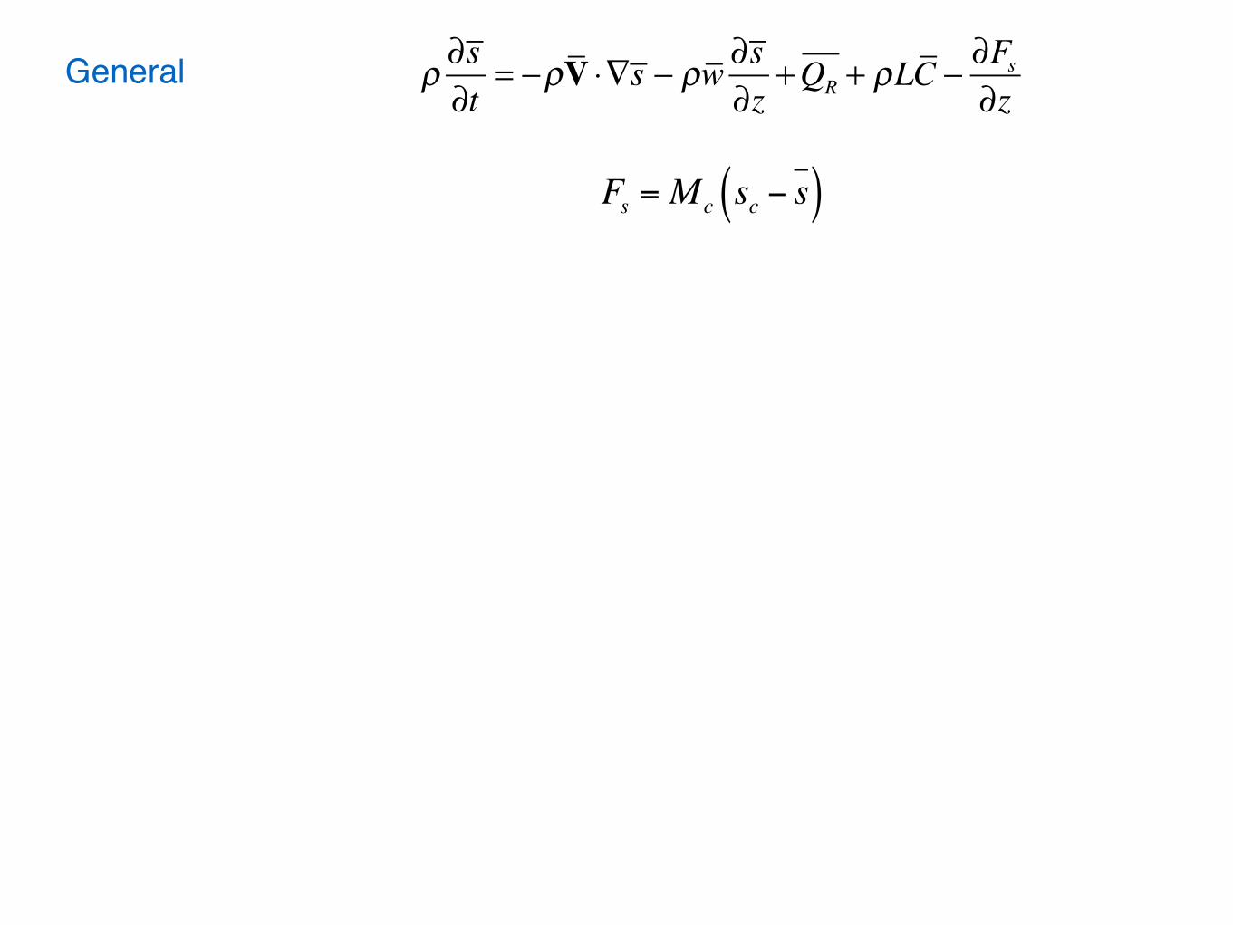
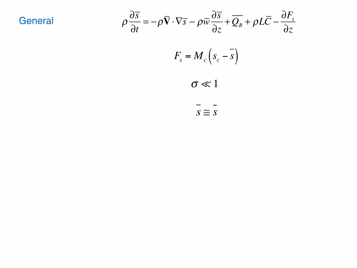
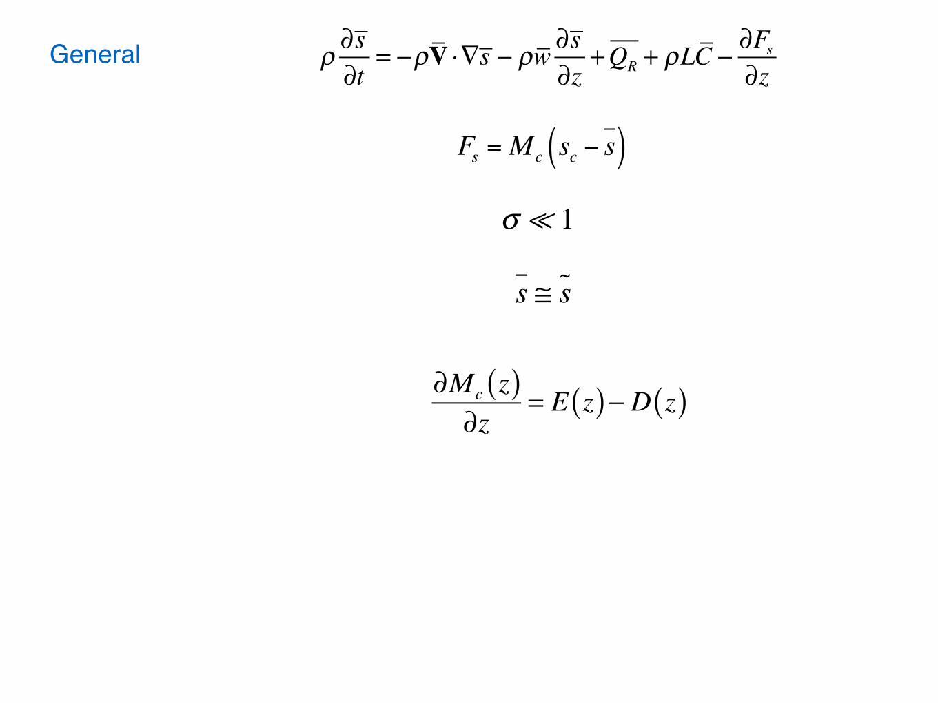
Step 1: Conversion to flux form

The original version of the CS parameterization was coded using the commonly used “compensating subsidence & detrainment” form of the equations.

That form is only valid for small sigma.

We therefore had to convert the code to the “flux divergence and source/sink” form, which is valid even for large sigma.

scale weather system. As pointed out by AS, the existence of such an area is a fundamental assumption of their theory. The area-averaged budget equations for mass, dry static energy, water vapor mixing ratio, and liquid water mixing ratio are:

0 = −∇⋅ ρV( )− ∂ ρw( )∂z

,

(56)

ρ ∂s∂t

= −ρV ⋅∇s − ρw ∂s∂z

+QR + ρLC − ∂Fs∂z

,

(57)

ρ ∂qv∂t

= −ρV ⋅∇qv − ρw ∂qv∂z

− ρC −∂Fqv∂z

,

(58)

ρ ∂l∂t

= −ρV ⋅∇l − ρw ∂l∂z

+ ρC − ∂Fl∂z

− χ .

(59)

Figure 6.12: Prof. Akio Arakawa, cruising along in mid-lecture.

! Revised Friday, January 30, 2009! 29

An Introduction to the Global Circulation of the Atmosphere

General


0 = −∇⋅ ρV( )− ∂ ρw( )∂z

,

(56)

ρ ∂s∂t

= −ρV ⋅∇s − ρw ∂s∂z


,

(57)

ρ ∂qv∂t



,

(58)

ρ ∂l∂t

= −ρV ⋅∇l − ρw ∂l∂z

+ ρC − ∂Fl∂z

− χ .

(59)




General

Fs =Mc sc − s( )

σ ≪ 1


0 = −∇⋅ ρV( )− ∂ ρw( )∂z

,

(56)

ρ ∂s∂t

= −ρV ⋅∇s − ρw ∂s∂z


,

(57)

ρ ∂qv∂t



,

(58)

ρ ∂l∂t

= −ρV ⋅∇l − ρw ∂l∂z

+ ρC − ∂Fl∂z

− χ .

(59)




General

Fs =Mc sc − s( )

s ≅ s!

σ ≪ 1


0 = −∇⋅ ρV( )− ∂ ρw( )∂z

,

(56)

ρ ∂s∂t

= −ρV ⋅∇s − ρw ∂s∂z


,

(57)

ρ ∂qv∂t



,

(58)

ρ ∂l∂t

= −ρV ⋅∇l − ρw ∂l∂z

+ ρC − ∂Fl∂z

− χ .

(59)




General

Fs =Mc sc − s( )

χ = 1−σ c( ) !χ +σ cχc .(90)

With these results, we can now rewrite (67) - (69) as

ρ ∂s∂t

= −ρV ⋅∇s − ρw ∂s∂z

+QR + ρL !C +σ cCc( )− ∂∂z

Mc sc − s( )⎡⎣ ⎤⎦ ,

(91)

ρ ∂qv

∂t= −ρV ⋅∇qv − ρw ∂qv

∂z− ρ !C +σ cCc( )− ∂

∂zMc qv( )c − qv⎡⎣ ⎤⎦{ } ,

(92)

ρ ∂l∂t

= −ρV ⋅∇l − ρw ∂l∂z

+ ρ !C +σ cCc( )− ∂∂z

Mc lc − l!( )⎡⎣ ⎤⎦ − 1−σ c( ) !χ +σ cχc⎡⎣ ⎤⎦ .

(93)

The convective condensation rate, Cc , appears in all three of these equations, as would be

expected.

A simple cumulus cloud model

To go further, we need to know the soundings inside the updrafts. For this, a simple cumulus cloud model is required. We assume that all cumulus clouds originate from the top of the PBL, carrying the mixed-layer properties upward. The mass flux changes with height according to

∂Mc z( )∂z

= E z( )− D z( ) .

(94)

Here E is the entrainment rate, and D is the detrainment rate. The in-cloud profile of moist static energy, hc z( ) , is governed by

∂∂z

Mc z( )hc z( )⎡⎣ ⎤⎦ = E z( )h! z( )− D z( )hc z( )

≅ E z( )h z( )− D z( )hc z( ) .(95)

There are no source or sink terms in (95) because the moist static energy is unaffected by phase changes and/or precipitation processes, and we neglect radiative effects. By combining (94) and (95), we can show that



s ≅ s!

σ ≪ 1


0 = −∇⋅ ρV( )− ∂ ρw( )∂z

,

(56)

ρ ∂s∂t

= −ρV ⋅∇s − ρw ∂s∂z


,

(57)

ρ ∂qv∂t



,

(58)

ρ ∂l∂t

= −ρV ⋅∇l − ρw ∂l∂z

+ ρC − ∂Fl∂z

− χ .

(59)




General

Fs =Mc sc − s( )

χ = 1−σ c( ) !χ +σ cχc .(90)


ρ ∂s∂t

= −ρV ⋅∇s − ρw ∂s∂z

+QR + ρL !C +σ cCc( )− ∂∂z

Mc sc − s( )⎡⎣ ⎤⎦ ,

(91)

ρ ∂qv


∂z− ρ !C +σ cCc( )− ∂

∂zMc qv( )c − qv⎡⎣ ⎤⎦{ } ,

(92)

ρ ∂l∂t

= −ρV ⋅∇l − ρw ∂l∂z

+ ρ !C +σ cCc( )− ∂∂z

Mc lc − l!( )⎡⎣ ⎤⎦ − 1−σ c( ) !χ +σ cχc⎡⎣ ⎤⎦ .

(93)


expected.



∂Mc z( )∂z

= E z( )− D z( ) .

(94)


∂∂z


≅ E z( )h z( )− D z( )hc z( ) .(95)




∂hc z( )∂z

=E z( )Mc

h z( )− hc z( )⎡⎣ ⎤⎦ .

(96)

This means that hc z( ) is affected by entrainment, which dilutes the cloud with environmental

air, but not by detrainment, which has been assumed to expel from the cloud air that has the cloud’s own moist static energy at each level.

Similarly, we can write

∂∂z

Mcsc( ) = Es − Dsc + ρσ cLCc ,

(97)

∂∂z

Mc qv( )c⎡⎣ ⎤⎦ = Eqv − D qv( )c − ρσCc ,

(98)

∂∂z

Mclc( ) = El!− Dlc + ρσ cCc − χc .

(99)

A simple microphysical model is needed to determine χc , i.e. to determine how much of

the condensed water is converted to precipitation, and the fate of the precipitation. The role of convectively generated precipitation, which drives convective downdrafts and moistens the lower troposphere by evaporating as it falls, is actually an important issue, but it will not be discussed here.

Compensating subsidence

By using (97)-(99), the large-scale budget equations can be rewritten in a very interesting way, as follows. First, consider the dry static energy. We write

∂∂z

Mc sc − s( )⎡⎣ ⎤⎦ =∂∂z

Mcsc( )−Mc∂s∂z

− s ∂Mc

∂z.

(100)

Substitute from (94) and (97) into (100), to obtain

∂∂z

Mc sc − s( )⎡⎣ ⎤⎦ = Es − Dsc + ρLσ cCc( )−Mc∂s∂z

− s E − D( )

= −Mc∂s∂z

− D sc − s( ) + ρLσ cCc .

(101)



s ≅ s!

σ ≪ 1


0 = −∇⋅ ρV( )− ∂ ρw( )∂z

,

(56)

ρ ∂s∂t

= −ρV ⋅∇s − ρw ∂s∂z


,

(57)

ρ ∂qv∂t



,

(58)

ρ ∂l∂t

= −ρV ⋅∇l − ρw ∂l∂z

+ ρC − ∂Fl∂z

− χ .

(59)




General

Fs =Mc sc − s( )

χ = 1−σ c( ) !χ +σ cχc .(90)


ρ ∂s∂t

= −ρV ⋅∇s − ρw ∂s∂z

+QR + ρL !C +σ cCc( )− ∂∂z

Mc sc − s( )⎡⎣ ⎤⎦ ,

(91)

ρ ∂qv


∂z− ρ !C +σ cCc( )− ∂

∂zMc qv( )c − qv⎡⎣ ⎤⎦{ } ,

(92)

ρ ∂l∂t

= −ρV ⋅∇l − ρw ∂l∂z

+ ρ !C +σ cCc( )− ∂∂z

Mc lc − l!( )⎡⎣ ⎤⎦ − 1−σ c( ) !χ +σ cχc⎡⎣ ⎤⎦ .

(93)


expected.



∂Mc z( )∂z

= E z( )− D z( ) .

(94)


∂∂z


≅ E z( )h z( )− D z( )hc z( ) .(95)




∂hc z( )∂z

=E z( )Mc

h z( )− hc z( )⎡⎣ ⎤⎦ .

(96)




∂∂z


(97)

∂∂z


(98)

∂∂z


(99)





∂∂z

Mc sc − s( )⎡⎣ ⎤⎦ =∂∂z


− s ∂Mc

∂z.

(100)


∂∂z


− s E − D( )

= −Mc∂s∂z


(101)



s ≅ s!

σ ≪ 1


0 = −∇⋅ ρV( )− ∂ ρw( )∂z

,

(56)

ρ ∂s∂t

= −ρV ⋅∇s − ρw ∂s∂z


,

(57)

ρ ∂qv∂t



,

(58)

ρ ∂l∂t

= −ρV ⋅∇l − ρw ∂l∂z

+ ρC − ∂Fl∂z

− χ .

(59)




General

This allows us to rewrite (91) as

ρ ∂s∂t

= −ρV ⋅∇s − ρw ∂s∂z

+QR + ρL !C +Mc∂s∂z

+ D sc − s( ) .

(102)

The last two terms on the right-hand side of (102) represent the cumulus effects, and the first of these in particular is quite interesting. It “looks like” an advection term. It represents the warming of the environment due to the downward advection of air from above, with higher dry static energies, by the environmental sinking motion that compensates for the rising motion in the cloudy updraft. The environmental sinking motion is often called “compensating subsidence,” because it compensates for the concentrated rising motion in the saturated updrafts. Up moist, down dry.

The role of compensating subsidence can be seen more explicitly by combining the two “vertical advection” terms of (92), and using (67), to obtain

ρ ∂s∂t

= −ρV ⋅∇s −M! ∂s∂z

+QR + ρLC" + D sc − s( ) ,

(103)

where

!M ≡ ρw −Mc

(104)

is the environmental mass flux. Why does !M appear in (103)? The reason is that the environmental subsidence is modifying !s , but s = !s . The last term on the right-hand side of (103) represents the effects of detrainment. You may be surprised to see that the cumulus condensation rate does not appear in (102) or (103). The reason is that condensation inside the updraft cannot directly warm the environment. Since almost the entire area is the environment, condensation in the updrafts does not, to any significant degree, directly affect the area-averaged dry static energy. Instead, the effects of condensation are felt indirectly, through the compensating subsidence term, which we have already explained. The physical role of condensation, then, is to make possible the convective updraft that drives the compensating subsidence, which in turn warms the environment. This is how condensation warms indirectly. Note that the vertical profile of the indirect condensation heating rate due to compensating subsidence is in general different from the vertical profile of the convective condensation rate itself.

In a similar way, we find that the water vapor budget equation can be rewritten as

ρ ∂qv

∂t= −ρV ⋅∇qv −M!

∂qv∂z

− ρC" + D qv( )c − qv⎡⎣ ⎤⎦ .

(105)



Fs =Mc sc − s( )

χ = 1−σ c( ) !χ +σ cχc .(90)


ρ ∂s∂t

= −ρV ⋅∇s − ρw ∂s∂z

+QR + ρL !C +σ cCc( )− ∂∂z

Mc sc − s( )⎡⎣ ⎤⎦ ,

(91)

ρ ∂qv


∂z− ρ !C +σ cCc( )− ∂

∂zMc qv( )c − qv⎡⎣ ⎤⎦{ } ,

(92)

ρ ∂l∂t

= −ρV ⋅∇l − ρw ∂l∂z

+ ρ !C +σ cCc( )− ∂∂z

Mc lc − l!( )⎡⎣ ⎤⎦ − 1−σ c( ) !χ +σ cχc⎡⎣ ⎤⎦ .

(93)


expected.



∂Mc z( )∂z

= E z( )− D z( ) .

(94)


∂∂z


≅ E z( )h z( )− D z( )hc z( ) .(95)




∂hc z( )∂z

=E z( )Mc

h z( )− hc z( )⎡⎣ ⎤⎦ .

(96)




∂∂z


(97)

∂∂z


(98)

∂∂z


(99)





∂∂z

Mc sc − s( )⎡⎣ ⎤⎦ =∂∂z


− s ∂Mc

∂z.

(100)


∂∂z


− s E − D( )

= −Mc∂s∂z


(101)



s ≅ s!

σ ≪ 1


0 = −∇⋅ ρV( )− ∂ ρw( )∂z

,

(56)

ρ ∂s∂t

= −ρV ⋅∇s − ρw ∂s∂z


,

(57)

ρ ∂qv∂t



,

(58)

ρ ∂l∂t

= −ρV ⋅∇l − ρw ∂l∂z

+ ρC − ∂Fl∂z

− χ .

(59)




General


ρ ∂s∂t

= −ρV ⋅∇s − ρw ∂s∂z


+ D sc − s( ) .

(102)



ρ ∂s∂t

= −ρV ⋅∇s −M! ∂s∂z

+QR + ρLC" + D sc − s( ) ,

(103)

where

!M ≡ ρw −Mc

(104)



ρ ∂qv

∂t= −ρV ⋅∇qv −M!

∂qv∂z

− ρC" + D qv( )c − qv⎡⎣ ⎤⎦ .

(105)



Fs =Mc sc − s( )

Restricted

χ = 1−σ c( ) !χ +σ cχc .(90)


ρ ∂s∂t

= −ρV ⋅∇s − ρw ∂s∂z

+QR + ρL !C +σ cCc( )− ∂∂z

Mc sc − s( )⎡⎣ ⎤⎦ ,

(91)

ρ ∂qv


∂z− ρ !C +σ cCc( )− ∂

∂zMc qv( )c − qv⎡⎣ ⎤⎦{ } ,

(92)

ρ ∂l∂t

= −ρV ⋅∇l − ρw ∂l∂z

+ ρ !C +σ cCc( )− ∂∂z

Mc lc − l!( )⎡⎣ ⎤⎦ − 1−σ c( ) !χ +σ cχc⎡⎣ ⎤⎦ .

(93)


expected.



∂Mc z( )∂z

= E z( )− D z( ) .

(94)


∂∂z


≅ E z( )h z( )− D z( )hc z( ) .(95)




∂hc z( )∂z

=E z( )Mc

h z( )− hc z( )⎡⎣ ⎤⎦ .

(96)




∂∂z


(97)

∂∂z


(98)

∂∂z


(99)





∂∂z

Mc sc − s( )⎡⎣ ⎤⎦ =∂∂z


− s ∂Mc

∂z.

(100)


∂∂z


− s E − D( )

= −Mc∂s∂z


(101)



s ≅ s!

σ ≪ 1


0 = −∇⋅ ρV( )− ∂ ρw( )∂z

,

(56)

ρ ∂s∂t

= −ρV ⋅∇s − ρw ∂s∂z


,

(57)

ρ ∂qv∂t



,

(58)

ρ ∂l∂t

= −ρV ⋅∇l − ρw ∂l∂z

+ ρC − ∂Fl∂z

− χ .

(59)




General


ρ ∂s∂t

= −ρV ⋅∇s − ρw ∂s∂z


+ D sc − s( ) .

(102)



ρ ∂s∂t

= −ρV ⋅∇s −M! ∂s∂z

+QR + ρLC" + D sc − s( ) ,

(103)

where

!M ≡ ρw −Mc

(104)



ρ ∂qv

∂t= −ρV ⋅∇qv −M!

∂qv∂z

− ρC" + D qv( )c − qv⎡⎣ ⎤⎦ .

(105)



So wewent back

Fs =Mc sc − s( )

Restricted

Do they give the same answers?

An example: One grid point on one time step.

-10 0 10 20 30 40 50 60Temperature tendency, K/day

200

300

400

500

600

700

800

900

1000

pres

sure

, hPa

90W, 6.7N

CStendMF-Cond

-20 -15 -10 -5 0 5Water vapor tendency, g/kg/day

200

300

400

500

600

700

800

900

1000

pres

sure

, hPa

90W, 6.7N

CStendMF-Cond

-10 0 10 20 30 40 50 60Temperature tendency, K/day

200

300

400

500

600

700

800

900

1000

pres

sure

, hPa

90W, 6.7N

CStendMF-Cond

OldNew

Step 2: Use the closure to calculate sigma

σ 1 =M 1( )E

ρδw1 + M 1( )E,

σ i = 1− σ jj=1

i−1

∑⎛

⎝⎜⎜

⎞

⎠⎟⎟


⎡

⎣⎢⎢

⎤

⎦⎥⎥for i = 2…N .

We already talked about this.


0 = −∇⋅ ρV( )− ∂ ρw( )∂z

,

(56)

ρ ∂s∂t

= −ρV ⋅∇s − ρw ∂s∂z


,

(57)

ρ ∂qv∂t



,

(58)

ρ ∂l∂t

= −ρV ⋅∇l − ρw ∂l∂z

+ ρC − ∂Fl∂z

− χ .

(59)




Step 3: Radiation and microphysics

Following Wu & Arakawa (2014), we area-weight the tendencies due to radiation and microphysics, including area-weighted contributions from updrafts, downdrafts, and the environment.

What the pieces look like

Temperature tendency Water vapor tendency Condensed water tendency

K day-1 g kg-1 day-1 g kg-1 day-1

CS convectionSAS shallow convectionLarge-scale microphysics

An example: One grid point on one time step.

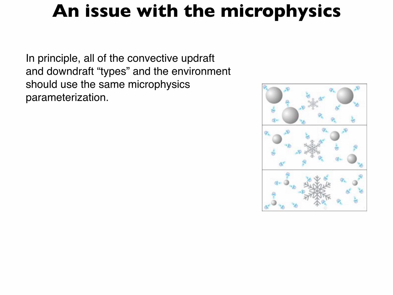
An issue with the microphysics

In principle, all of the convective updraft and downdraft “types” and the environment should use the same microphysics parameterization.



With a state-of-the-art microphysics parameterization, the cost would be prohibitive.




We have used the standard GFS microphysics parameterization for the environment, and a highly simplified scheme for the convective updrafts and downdrafts.




We have used the standard GFS microphysics parameterization for the environment, and a highly simplified scheme for the convective updrafts and downdrafts.

A better solution is needed.

Sigma increases at higher resolutionUpdraft area fraction log(PDF), 30S-30N: T62

0 0.1 0.2 0.3 0.4 0.5

100

200

300

400

500

600

700

800

900

1000

Pres

sure

, mb

-6

-5

-4

-3

-2

-1

0

Updraft area fraction log(PDF), 30S-30N: T126

0 0.1 0.2 0.3 0.4 0.5

100

200

300

400

500

600

700

800

900

1000

Pres

sure

, mb

-6

-5

-4

-3

-2

-1

0


0 0.1 0.2 0.3 0.4 0.5

100

200

300

400

500

600

700

800

900

1000

Pres

sure

, mb

-6

-5

-4

-3

-2

-1

0


0 0.1 0.2 0.3 0.4 0.5

100

200

300

400

500

600

700

800

900

1000

Pres

sure

, mb

-6

-5

-4

-3

-2

-1

0

These plots are for the sum of sigma over all cloud types. The zeros for grid cells without convection are included in the pdfs. Twelve separate time-slices over 24 hours have been used to cover the diurnal cycle.

T574 Sandy Forecasts

Sandy minimum pressure Sandy track

Future work

Move to NGGPS

Test at higher resolution

Find a better compromise for the microphysics

Conclusions

• The Unified Parameterization has a closure for sigma rather than a closure for the mass flux.

• We have generalized the closure to work with a spectrum of updrafts and downdrafts.

• We have tested the parameterization in the GFS, using the Chikira-Sugiyama parameterization as a base.

• Future work should include improving the consistency of the cloud microphysics across updrafts, downdrafts, and environment.

Documents

Testing a Resolution-Independent Parameterization of Deep