Test Taking Strategies in Computer Adaptive Testing that

Test Taking Strategies in Computer Adaptive Testing that will Improve Your Score:

Fact or Fiction?

Jennifer L. Ivie

Submitted to the Department of Psychology

and the faculty of the Graduate School of the University of Kansas

in partial fulfillment of the requirements for the degree of Doctor of Philosophy

_______________________________________ Co-Chair _______________________________________ Co-Chair _______________________________________ _______________________________________ _______________________________________ Date defended: _________________________

ii

The Dissertation Committee for Jennifer L. Ivie certifies that this is the approved version of the following dissertation:

Test Taking Strategies in Computer Adaptive Testing that will Improve Your Score: Fact or Fiction?

Committee: _______________________________________ Co-Chair

_______________________________________

Co-Chair

Date approved _________________

iii

ABSTRACT

Jennifer L. Ivie, Ph.D. Department of Psychology

University of Kansas

The purpose of this study was to examine the validity of the claim made by test

review companies that spending more time and attention on the first five or ten items

on a computer adaptive test will improve an examinee’s final ability estimate. Study 1

examined the effects of different amounts of information about how the test works

and/or how to improve your score. In this study, it was found that having information

on how to perform better on an exam does result in higher scores. Study 2 was a

series of simulation studies that examined the stability of a computer adaptive test and

the actual theta estimate when certain test parameters were varied: item bank

parameters (item pool size, discrimination parameters, and guessing parameters);

examinee parameters (whether or not the examinee has an artificially boosted ability

level); and testing algorithm parameters, in particular how the first items are selected.

Overall, evidence was found to support this test taking strategy taught to improve test

scores. Finally, these results were compared to current average GRE scores for

graduate schools across the United States. It was found that this artificial boost can

result in admittance when the true theta might have resulted in non-admittance.

iv

Acknowledgments

Blah blah blah

v

Table of Contents

1. Introduction………………………………………………………………1

Literature Review……………………………………………………..

2.1 Item Response Theory………………………………………………...

2.1.1 IRT Assumptions…………………………………………………………….

2.1.2 Item calibration……………………………………………………………..

2.1.3 Person calibration………………………………………………………….

2.1.4 Joint Person and Item Calibration……………………………………….

2.1.5 The role of IRT in CAT…………………………………………………….

2.1.5.1 Ability level estimation………………………………………….

2.1.5.2 Item bank development………………………………………….

2.2 Computerized Adaptive Testing………………………………………..

2.2.1 Introduction………………………………………………………………….

2.2.2 The procedure……………………………………………………………….

2.2.2.1 Step 1 – The starting rule……………………………………….

2.2.2.2 Step 2 – The continuation rule…………………………………

2.2.2.3 Step 3 – The stopping rule……………………………………...

2.2.3 Previous Research on CAT………………………………………………..

2.2.3.1 Technical issues within CAT…………………………………...

2.2.3.2 Practical issues within CAT……………………………………

2.2.3.3 Research and development of the CAT-ASVAB……………...

2.3 Abstract Reasoning Test

vi 2.3.1 What is intelligence?

2.3.2 Measures of Intelligence

2.3.2.1 Raven’s Progressive Matrices

2.3.2.2 Abstract Reasoning Test

2.4 Conclusion

3. Study 1

3.1 Methods

3.1.1 Participants

3.1.2 Materials and Apparatus

3.1.2.1 Item Pool

3.1.2.2 Testing Program

3.1.2.3 Instructions

3.1.3 Procedure

3.2 Results

3.2.1 Descriptive Statistics

3.2.2 Inferential Statistics

3.3 Discussion

4. Study 2

4.1 Methods


4.1.2 Starting rules

4.1.3 Continuation rule

vii 4.1.4 Stopping rule

4.1.5 Data Generation

4.1.5.1 Item parameter generation

4.1.5.2 Examinee parameter generation

4.1.5.3 Adaptive test generation

4.1.6 Outcome Measures

4.2 Results

4.2.1 Descriptive Statistics for Final Theta Estimation

4.2.2 Overall Differences in Dependent Variables

4.2.2.1 Root mean squared error

4.2.2.2 Bias

4.2.2.3 Standard deviation

4.2.3 Null versus Boost Conditions


4.2.3.2 Bias


4.2.4 Condition Type


4.2.4.2 Bias


4.2.5 Item Pool Size

4.2.5.1 Root mean squared deviation

viii

4.2.5.2 Bias


4.2.6 Discrimination Parameter Levels


4.2.6.2 Bias


4.2.7 Guessing Parameter Levels


4.2.7.2 Bias


4.2.8 Differences between True Theta Levels


4.2.8.2 Bias


4.3 Discussion

5. Conclusion

References

Appendix A

Appendix B

Appendix C

Appendix D

ix

List of Tables

Table 3.1. Descriptive statistics for Study 1 (after removing outliers)……..

Table 3.2. Crosstabs analysis of the proportion of each sample (and

number of participants from each sample) who answered

yes/no to the questions regarding prior exposure to a CAT..……….

Table 3.3. Planned comparison significance tests and effect sizes for

each dependent variable…………………………………………………..

Table 4.1. Descriptive statistics for ability level boosts for items 1

through 10.………………………………………………………….

Table 4.2. Descriptive statistics for average GRE-Q and GRE-V scores

for 340 graduate programs broken down by selection ratio………..

x

List of Figures

Figure 2.1. Example ICCs for five items……………………………………..

Figure 2.2. Flowchart representing an adaptive test (adapted from …………

Thissen & Mislevy, 2000)

Figure 2.3. Examples of each of the five rules for solving RPM test items…

Figure 3.1. Example Abstract Reasoning Test item similar to those ………..

created for Study 1. The correct answer is 3

Figure 4.1. Spaghetti plot of mean ability level boost for each theta level…..

for Items 1 through 10

Figure 4.2a. Average theta estimate for boost condition at each theta ……….

interval at each item interval of the test

Figure 4.2b. Standard deviation of the theta estimate for boost conditions at

each theta interval at each item interval of the test

Figure 4.3. Estimated marginal means for RMSE for the null versus boost

conditions over the 35 item test

Figure 4.4. Estimated marginal means for the bias between the null and boost

conditions

Figure 4.5. Estimated marginal means for differences in standard deviation

between null and boost conditions

Figure 4.6a. Estimated marginal means for the root mean squared error for each

null condition type for items over the test

xi Figure 4.6b. Estimated total root mean squared error for each boost condition

type for items over the test

Figure 4.7a. Estimated marginal means for the RMSE at each item interval

for the linear test null conditions

Figure 4.7b. Estimated marginal means for the RMSE at each item interval

for the linear test boost conditions

Figure 4.8a. Estimated marginal means for bias between condition types for

the null conditions

Figure 4.8b. Estimated marginal means for bias between condition types for

the boost conditions

Figure 4.9a. Estimated marginal means for bias between linear fixed test

conditions for null conditions.

Figure 4.9b. Estimated marginal means for bias between linear fixed test

conditions for boost conditions

Figure 4.10a. Estimated marginal means for standard deviation between

condition types for null conditions

Figure 4.10b. Estimated marginal means for standard deviation between

condition types for boost conditions

Figure 4.11a. Estimated marginal means for standard deviation between linear

test types for null conditions

Figure 4.11b. Estimated marginal means for standard deviation between linear

test types for boost conditions

xii Figure 4.12a. Estimated marginal means for RMSE for the item pool size for

the null conditions

Figure 4.12b. Estimated marginal means for RMSE for the item pool size for

the boost conditions

Figure 4.13a. Estimated marginal means for standard deviation between item

pool sizes for null conditions

Figure 4.13b. Estimated marginal means for standard deviation between item

pool sizes for boost conditions

Figure 4.14a. Estimated marginal means for RMSE between discriminating

parameters for the null conditions

Figure 4.14b. Estimated marginal means for RMSE between discriminating

parameters for the boost conditions

Figure 4.15a. Estimated marginal means for bias between discrimination

parameter levels for null conditions

Figure 4.15b. Estimated marginal means for bias between discrimination

parameter levels for boost conditions


discrimination parameter levels for null conditions


discrimination parameter levels for boost conditions

Figure 4.17a. Estimated marginal means for the RMSE between guessing

parameters for the null conditions

xiii Figure 4.17b. Estimated marginal means for the RMSE between guessing

parameters for the boost conditions

Figure 4.18a. Estimated marginal means for bias between guessing parameter

levels for null conditions

Figure 4.18b. Estimated marginal means for bias between guessing parameter

levels for boost conditions

Figure 4.19a. Estimated marginal means for standard deviation between guessing

parameter levels for null conditions

Figure 4.19b. Estimated marginal means for standard deviation between guessing

parameter levels for boost conditions

Figure 4.20a. Estimated marginal means for root mean squared error for each true

theta level across the test for the null conditions

Figure 4.20b. Estimated marginal means for root mean squared error for each true

theta level across the test for the boost conditions

Figure 4.21a. Estimated marginal means for bias throughout the test for each true

theta level for the null conditions

Figure 4.21b. Estimated marginal means for bias throughout the test for each true

theta level for the boost conditions

Figure 4.22a. Estimated marginal means for squared deviation throughout the test

for each true theta level for the null conditions

Figure 4.22b. Estimated marginal means for squared deviation throughout the test

for each true theta level for the boost conditions

xiv Figure 4.23. GRE-V scores for all true theta values compared to average GRE-V

scores corresponding to each college selection ratio

Figure 4.24. GRE-Q scores for all true theta values compared to average GRE-Q

scores corresponding to each college selection ratio

1

1. Introduction

High stakes testing is a large area of research and debate in today’s society,

especially in the United States. With most institutions of higher education requiring

the reporting of test scores, such as the GRE, SAT, ACT, LSAT, MCAT, etc.,

students spend a lot of time worrying about and studying for these tests prior to

application into institutions of higher education. Many of these students will do

anything necessary or suggested to improve their scores on these exams, often paying

hundreds of dollars to tutors and/or test review companies for classes or books that

are supposed to help students prepare for these tests. Many of these tests have more

recently become computer adaptive (CAT), a format that is administered on a

computer and adapts itself to the apparent ability level of the examinee.

The purpose of this study is to examine a particular test taking strategy taught

by such test review companies that claim the strategy will improve the overall score

for the individual on such a computer adaptive test. This strategy involves paying

more attention to the items at the beginning of the test. This includes spending more

time on these items, sacrificing the items near the end of the test. The claim is made

that the adaptive nature of the test is such that larger changes or adaptations are made

earlier in the test as the program is attempting to narrow in on an examinee’s ability

level. Thus, it is easier for an examinee to improve his/her score at this point in the

test. Later in the test, it is claimed that these jumps are smaller and thus will result in

less change in the ability estimate. This claim was tested through two studies looking

at the problem from two different perspectives.

2

The goal of the first study was to examine the possibility that examinees who

have learned this test taking strategy will score higher on an adaptive test than their

counterparts who have not been taught the strategy. To reach this goal, college-aged

participants were administered a computer adaptive abstract reasoning test. Some of

the participants were taught the strategy while others were not.

This first study aimed to find differences due to knowledge of a strategy to

“beat” the test. It could be hypothesized that just knowledge on that a person can beat

a test will improve his/her score because it will lower test anxiety and increase test

motivation. Research has also shown that test anxiety and test performance have an

indirect relationship (Shermis & Lombard, 1998). Research has shown a direct

relationship between test motivation and test performance (Kim & McLean, 1995;

Cohen, 1998). found that increased test motivation improved test scores. Finally,

research has shown that strategy training has a direct relationship with test

performance (Embretson, 1992).

The goal of the second study was to examine the stability of a computer

adaptive test at different places throughout the test to examine the claim that larger

jumps are made earlier in the test, with smaller jumps later in the test. Also, in the

second study, differences in final ability estimates between subjects with some sort of

artificial boost (in terms of this series of studies, the artificial boost refers to

knowledge on how to beat the test) and those without this boost in ability level was

examined under varying testing algorithm conditions. This goal was reached using a

CAT simulator that simulated examinee responses to items that were selected and

3 “administered” through adaptive procedures. The adaptive algorithm was varied on

starting rule (i.e., how the first item(s) was selected), item discrimination and

guessing parameter levels, and item pool size. Simulated participants’ true ability

levels ranged from -3.25 to 3.25.

Research has been conducted on the role of the starting rule used in a CAT

algorithm. Much of this research has focused on issues of test security rather than the

affect on test stability. Arguments have been made for randomly selecting the first

item from a particular number of items or particular item difficulty range (Hulin,

Drasgow, & Parsons, 1983; Embretson & Reise, 2000). Others have argued for an

extension of the previous suggestion—that is, to randomly select the first 5 or 10

items from a given number of items (McBride, Wetzel & Hetter, 2001). Finally,

others have argued for fixed testlets that could be used at the beginning of a CAT

(Wainer & Kiely, 1987).

Many researchers have examined the affects of differing discrimination and

guessing parameters on the accuracy of ability estimates in a computer adaptive

framework (e.g., Vale & Weiss, 1975; Urry, 1974, 1975; Jensema, 1974; Chang,

1999; and Hau & Chang, 2001). Most research has shown that higher discrimination

parameters and lower guessing parameters are ideal. Finally, research has shown that

larger item pools are better in terms of ensuring more accurate ability estimates

(Embretson & Reise, 2000).

As stated above, the purpose of this set of studies is to examine the efficacy of

a commonly taught test taking strategy for high-stakes computer adaptive tests. In

4 Chapter 2 previous research on issues related to the purpose of this study are outlined

including: the history of adaptive testing, previous research on the development and

administration of computer adaptive tests, the item response theory concepts utilized

by CAT algorithms, and information on the abstract reasoning test used in Study 1. In

Chapter 3 and 4 the methods, results and discussion of Study 1 and Study 2

(respectively) are described. And, finally, the overall conclusions are discussed in

Chapter 5.

5

2. Literature Review

Written proficiency testing became widespread throughout the United States

and Western Europe in the mid-nineteenth century. In the early 1900s, testing began

the shift from individualized testing to mass testing. This allowed for more efficient

testing and more homogenous testing environments. In a paper-and-pencil group

testing situation, the entire group receives the same items. As a result, enough items

of all proficiency levels must be present on the exam to ensure close estimation of

person parameters for all people taking the test. However, most paper-and-pencil

(P&P) exams have a majority of items near average proficiency levels because most

of the population falls within two standard deviations of the average proficiency

level. In addition, ensuring valid and reliable P&P tests requires test developers to

include a large number of items on the test (Wainer, 2000).

Creating more accurate and reliable P&P tests typically includes adding more

items to the test at different ability levels. For this reason, as well as others which I

will expand upon later, research on adaptive testing formats began as early as the

1950’s. The first sign of adaptive testing was in the late 1950s, 1960s and early 1970s

when several kinds of branching tests were designed. These were tests for which trees

of items were developed that branched from one item to the next based on the

examinee’s answer to the previous item, that is whether or not the examinee answered

the item correctly (Krathwol & Huyser, 1956; Hansen, 1969; and Hulin, Drasgow &

Parsons, 1983). While many of today’s adaptive tests are computer-based, many early

6 inventive formats were developed to implement adaptive procedures without the use

of computers.

In the early 1970’s researchers began developing and examining testing

systems that allowed a examinee to take a shorter test with better measurement

precision by giving examinees items based on their estimated proficiency level. Four

examples of these sorts of tests include the flexilevel test (Lord, 1971a), the two-stage

test (Lord, 1971b), the pyramidal test (Larkin & Weiss, 1974, as cited in McBride,

2001b), and a stratadaptive test (Weiss, 1974, as cited in McBride, 2001b). Each of

these tests, as well as other predecessors of the computer adaptive test, will be

discussed now.

Lord (1971a) designed a P&P test called the self-scoring flexilevel test which

required the examinee to adjust their progress based on the accuracy of their answers.

This test requires complex instructions because the adjusted scoring is the job of the

examinee. On the other hand, this test allows for adaptive testing without the use of

computationally complex scoring algorithms (Thissen & Mislevy, 2000). In the

flexilevel test, each examinee responds to half of the items on the complete test. The

selected half of the items depends on the examinee’s proficiency level; difficult items

are answered by more proficient examinees while easier items are answered by the

less proficient.

An example of a flexilevel test is as follows. Items are ordered by difficulty

level on a two-column sheet of paper with the item of middle difficulty centered at

the top of the page, the more difficult items listed in the right-hand column increasing

7 in difficulty, and the easier items listed in the left-hand column decreasing in

difficulty. The examinee begins with the middle difficulty question at the top of the

page. The examinee marks the sheet, if they answer correctly, the answer turns a

particular color signifying he/she to proceed to the first item in the more difficult

column. If the examinee answers incorrectly, the color shown signifies to proceed to

the first item in the easier column. The examinee then proceeds to the next available

item in the column signified by the color shown with each answer. All examinees

answer the same number of questions, and their final score is based on the difficulty

of the last item answered (Lord, 1971a). Simply put, each time an examinee answers

a question, he or she is routed to an easier or harder item based on the correctness of

his/her previous answer (Schoonman, 1989).

Olivier (1974) conducted a study comparing the flexilevel test to conventional

P&P tests. He found that the flexilevel test had lower reliability and validity than the

conventional test. He also found about 15 percent of the examinees who took the

flexilevel test had to be removed from the study due to errors made in the self-scoring

mechanism (as cited in McBride, 2001b). Betz and Weiss (1975) also compared the

flexilevel test to a conventional test. However, unlike the previous study, the tests

were administered on the computer to remove self-scoring errors. In this study, they

found that both tests demonstrated the same degree of test-retest reliability (as cited in

McBride, 2001b).

The two-stage adaptive testing system, another predecessor proposed by Lord

(1971b), involves giving examinees two sets of items. The examinee’s performance

8 on the first set of items decides whether he/she will receive the harder or easier

second set of items. Betz and Weiss (1973) compared a computer-based, conventional

40-item test, to a computer-based, two-stage test with two 20-item sets. They found

similar test-retest reliability between these two types of tests. Possibly degrading

these results, they also found that the first set of items in the two-stage test were too

easy for the sample of examinees used in this study (as cited in McBride, 2001b).

Another testing system that utilizes this adaptive concept is that of a fixed

branching system. This system is known as pyramidal or staircase adaptive testing

(Larkin & Weiss, 1974). In a test of this type, one item is always the starting point.

This item branches into two other items: one harder and one easier. These items

branch into two more items each—one harder and one easier per item—continuing on

to result in a lattice-like branching system. This continues on for as many levels as the

number of items the test developer would like the examinee to answer. This differs

from the systems of interest in this study because the branching order is pre-specified

and everyone with the same response pattern receives the same items.

There are some important disadvantages to the pyramidal testing system. One

major disadvantage is the enormous number of items required. If an administrator

wants the examinees to answer n items, the number of items necessary for the

branching system is equal to (2n – 1). Thus, an 8 item test would require 255 items.

Another disadvantage is that the first few items in the test would have much higher

exposure rates than the items at the end of the test, leading to decreased security on

these items, which could also lead to inflated final scores. Also, if an examinee makes

9 simple errors on the first few items by answering the first couple of items incorrectly,

he/she cannot increase his/her score beyond this lower set of items. This is a major

drawback of any fixed-item selection adaptive testing system (Schoonman, 1989).

Larkin and Weiss (1974) compared this test to the two-stage test discussed

previously. They found both tests to have comparable test-retest reliability, but they

found that the two-stage test resulted in higher proportion correct scores due to the

tailoring properties of the test (as cited in McBride, 2001b).

Similar to the pyramidal test, with a prespecified branching system, the

stratadaptive (or stratified adaptive) method branches from one set of items to

another, rather than from one item to another. In this method, proposed by Weiss

(1974), the item pool must first be sorted into strata, or mutually exclusive groups,

based on item difficulty. Rather than branching from one item to the next depending

on correctness of answer, the test branches (in the same manner as the pyramidal test)

from one strata to the next. The examinee is given only one item from each strata. In

the original design, Weiss (1974) proposed this test as a variable length, variable

entry test. Waters (1974) conducted a study comparing three forms of the

stratadaptive test to a conventional computer based test. He found the reliability and

external validity to be higher for the stratadaptive tests than for the conventional test.

He also found these tests to be 36 to 60 percent shorter on average than the 50-item

conventional test.

Vale and Weiss (1975) also conducted an empirical study comparing the

stratadaptive test to the conventional test. They found the stratadaptive test to be 34%

10 shorter than the conventional test. Also, they found the stratadaptive test to have

higher internal consistency (.94 versus .91), and similar test-retest reliability. They

followed this empirical study with a simulation study in which they systematically

varied item discriminations, test length, and the availability and quality of prior

examinee ability information. They conducted separate studies of fixed and variable

length tests. In the fixed length test simulation study, they found the fidelity

coefficient for the peaked conventional test to be superior to that of the stratadaptive

test for items with low discriminating power (α = .50). However, at the higher levels

(α = 1.0 and 2.0), the stratadaptive test had higher fidelity than the conventional test.

In the variable length studies, they found similar results. At the lower discriminating

items (α = .50 and 1.0), they found that the stratadaptive test had lower fidelity

coefficients than the conventional, even with more than 40 items. Yet, at the high

discrimination parameters (α = 2.0), they found much higher fidelity coefficients for

the stratadaptive tests even though the tests were much shorter (28 items) than the 40-

item conventional test (as cited in McBride, 2001b).

Another early adaptive testing system is the Implied Orders Tailored Testing,

originally developed by Cliff (1975). While this method is more valid than the fixed

item selection methods discussed above, it lacks the psychometric model of the

outcome when a person of a certain proficiency level meets an item with certain

characteristics; this method as well as the others mentioned above does not utilize the

IRT methods used by current CAT systems to explain the interactions between

persons and items (Cudeck, McCormick, & Cliff, 1980; Schoonman, 1989). Thus,

11 further research was conducted in attempts to utilize these IRT methods to better

adjust item administration to the proficiency level of the examinee.

Based on the principles of this new testing system, in the early 1980s military

researchers began creating computer-based tests that would choose items at the

appropriate proficiency level for the examinees. The tests would administer items

based on the accuracy of the previously answered items and adapt themselves to the

examinee’s performance. Thus, they have been named Computer Adaptive Tests or

CATs (Wainer, 2000). Unlike these previous tests, these new systems would utilize

IRT methods for scoring tests and choosing items. They found that utilizing CAT

methodology in their recruitment testing procedure would improve the person-job

match due to increased validity of the test. This 12-year military research project

which began in 1979 on CAT (Martin & Hoshaw, 2001) will be expanded upon in

later sections. While this was the first large scale CAT research program, other

smaller CAT research programs will also be discussed in future sections.

Due to this wealth of research, CATs are beginning to replace traditional P&P

tests in many fields of measurement. In education, research on converting the GRE to

CAT form began in the late 1980’s (Schaeffer et al., 1995). As well, tests like the

Graduate Management Admissions Test (GMAT) is currently in CAT form. In

psychology, cognitive measures (e.g., the ART developed by Embretson, 2005) as

well as personality measures have been transferred to computer format. In the

medical field, some questionnaires have been developed in CAT form (e.g., the HIT

12 developed by Bjorner, Kosinski & Ware, 2003). As mentioned above, in the military,

the largest high stakes CAT program has been developed (CAT-ASVAB).

Computer adaptive tests have many advantages over the traditional P&P tests:

shorter tests, enhanced measurement precision, testing on demand, and immediate test

scoring and reporting, to name a few (Meijer & Nering, 1999). In terms of test

construction, computer-administration of tests allows for easy pilot testing of new

items and immediate removal of faulty items. Another advantage to a CAT is that,

because it is administered on the computer, graphics, sounds, running video, and text

can be combined to present tasks that resemble real-life tasks (Green, 1983). It is

important to note that the first advantage, shorter tests, might seem contradictory to

the fundamental principle of test development which states that longer tests provide

more reliable estimates of trait level. But, because of the IRT procedure that is

followed in a CAT, the proficiency level is more accurately estimated with fewer

items (Straetmans & Eggen, 1998). I will outline this procedure in the next section.

Considering the advantages of CAT over traditional P&P tests, there are still

some practical aspects that can be seen as disadvantages to examinees who are used

to P&P tests. First, while computers are becoming more and more available in today’s

society, many examinees are still unfamiliar with the use of computers which could

give them a disadvantage over those who are familiar with the computer. A second

possible disadvantage of CAT when compared with P&P tests is that examinees are

no longer given all items at one time allowing them to return to items they might have

skipped or to change their answers on items they have already attempted. Rather, they

13 are given one item at a time, and must choose a final answer before continuing on to

the next item. Another possible disadvantage to taking the test in the CAT format is

one of motivation and anxiety—if the examinees understand the process the computer

goes through to pick subsequent items, and they are given an item that they consider

to be easy, they could assume they got the previous question incorrect. This could

affect their future performance on the test.

Part of this knowledge about the inner workings of CATs comes from training

courses and books like those put out by Princeton Review and Kaplan. One piece of

advice that is given by these companies, especially for taking high stakes tests like the

GRE, is that “one of the most important things to know is that the first few questions

are the most important on the test (Kaplan, 1997, pp. 174).” They continue on to

explain how paying extra attention to the first “five or so” problems, leaving the later

questions to guessing if necessary, will improve your score. This is based on the

assumption that earlier in the test bigger adjustments are made to the estimated

proficiency level and increasing your score at the beginning makes it more difficult to

get a lower score than starting off with a lower score and returning to a higher score

in the end. Or as Princeton Review (Still, 2003) states it:

“The computer weighs your performance on earlier questions more heavily

than it does later ones. Early in the test, your score will move up and down

(hopefully, up!) in large increments, but as you near the end, your score will

change only by small amounts…This means you’ll need to concentrate

hardest on answering the early questions correctly, even if this means

14

spending more time on them than you’d like. You can make this time up by

moving more quickly on later questions, when you’ll affect your score less

dramatically (p. 10-11).”

This test-taking strategy leads to multiple questions. Will an examinee get a

better overall score if they only get the first items correct versus a steadier pattern of

correctness throughout the test? Or in a more real-world sense, will an examinee get a

better overall score if they pay much closer attention to the first items on the test

giving them a sort of boost in their proficiency level earlier on the test? This question

is important to the testing community because of the impact it will have on test taking

strategies as more and more tests become computer adaptive. These questions were

the focus of this set of studies.

I have briefly outlined the advantages and disadvantages to using a CAT

system for testing, as well as some of the history of adaptive testing. The rest of this

chapter will focus first on the psychometric theory behind a working CAT, including

the Item Response Theory (IRT) methodology underlying this system. Secondly, it

will look at the actual procedure that the testing algorithm follows when

administering a CAT, as well as some of the issues in test design that affect this

process. The third section will be dedicated to studies that have been conducted on

CATs: for example, human factors and computer adaptive testing and simulation

studies on particular testing algorithms. Finally, there will be a short section that

focuses on the Abstract Reasoning Test that is currently in CAT form.

15

2.1 Item Response Theory

In a traditional P&P test, in line with Classical Testing Theory (CTT), a

person’s proficiency score is usually number correct or some linear transformation of

number correct. With a CAT, examinees receive different items, and in some CATs

even a different number of items. Some examinees receive harder items while others

receive easier items. Thus, it would be inequitable if examinees receive scores based

solely on number of correct responses. To deal with this problem, Item Response

Theory (IRT) is used to calculate scores. Item Response Theory “presents a

mathematical characterization of what happens when an individual meets an item

(Wainer, 2000, pp. 12)”; IRT is a mathematical modeling methodology that allows

researchers to compare a person’s proficiency with the item’s difficulty in order to

predict the probability of a correct response on the item (Wainer, 2000).

One major advantage to IRT methods over CTT methods is parameter

invariance. In CTT, the proportion correct or easiness parameter of an item is based

solely on the subpopulation that took the test. The methods used to estimate item and

person parameters in IRT remedy this dependence. The property of parameter

invariance refers to the independence of the ability distribution of the examinees from

the item parameters, that is the true value estimation of the person’s proficiency level

is not dependent on the particular set of test items administered and an item’s true

value parameters are not the result of the subpopulation of examinees used to estimate

these parameters (Hambleton, Swaminathan & Rogers, 1991).

16 In summary, IRT is a model-based methodology that can be used to estimate

the parameters of each item in an item pool, a person’s proficiency level, the

reliability and precision of a test, as well as the validity of the item selection

algorithm (Wainer, 2000). IRT also allows us to deal with three challenges in

adaptive testing. The first is to find a useful way to characterize the variation among

items in the item pool. The second challenge is to determine efficient rules for item

selection during test administration. The third challenge is arriving at proficiency

scores on a common scale regardless of the subset of items the examinees received

(Wainer & Mislevy, 2000).

2.1.1 IRT Assumptions

Before getting into the particulars of the methodology, I will discuss the

assumptions that must be met when using IRT: item fungibility, test

unidimensionality, local item independence, known item parameters, and no

differential item functioning (DIF). The first assumption, item fungibility, relates to

the order of the items. This assumption states that regardless of the order in which

you present the items, the person’s proficiency estimate should not be affected

(Wainer & Mislevy, 2000).

Unidimensionality refers to the assumption that all items in the test (or

subtest) measure only one ability or trait. This assumption is never strictly met due to

outside cognitive, personality, and test-taking factors that can affect test performance.

(If there are other significant factors playing a role in the measure, they can be

modeled using Multidimensional Item Response Theory (MIRT).) For purposes of

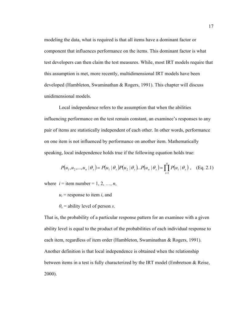
17 modeling the data, what is required is that all items have a dominant factor or

component that influences performance on the items. This dominant factor is what

test developers can then claim the test measures. While, most IRT models require that

this assumption is met, more recently, multidimensional IRT models have been

developed (Hambleton, Swaminathan & Rogers, 1991). This chapter will discuss

unidimensional models.

Local independence refers to the assumption that when the abilities

influencing performance on the test remain constant, an examinee’s responses to any

pair of items are statistically independent of each other. In other words, performance

on one item is not influenced by performance on another item. Mathematically

speaking, local independence holds true if the following equation holds true:

( ) ( ) ( ) ( ) ( )∏=

==n

isisnsssn uPuPuPuPuuuP

12121 ||...|||,...,, θθθθθ , (Eq. 2.1)

where i = item number = 1, 2, …, n,

ui = response to item i, and

θs = ability level of person s.

That is, the probability of a particular response pattern for an examinee with a given

ability level is equal to the product of the probabilities of each individual response to

each item, regardless of item order (Hambleton, Swaminathan & Rogers, 1991).

Another definition is that local independence is obtained when the relationship

between items in a test is fully characterized by the IRT model (Embretson & Reise,

2000).

18 The local independence assumption can also be called conditional

independence. This name refers to the fact that the independence of item responses is

only considered independent after you take into consideration the person’s ability

level. In other words, after you statistically partial out the ability level, the examinee’s

responses should be independent; an examinee’s responses are independent after

conditioning on ability (Hambleton, Swaminathan & Rogers, 1991).

There are three IRT models that will be focused on in this paper: the one-,

two- and three-parameter logistic models. The next assumption requires that the item

parameters required for each model are known, and that these item parameters are the

only item parameters that influence examinee performance on that item (Hambleton,

Swaminathan & Rogers, 1991). This assumption can also be described in terms of the

item characteristic curve (ICC). The ICC is a non-linear probability distribution that

demonstrates the relationship between ability level and probability of a correct

response on the item. This assumption states that the ICC has a specified form,

determined by the item parameter(s) in the model (Embretson & Reise, 2000).

The final assumption that should be met for each item is that items must

display no differential item functioning (DIF). That is, an item must perform the same

for each person regardless of the subgroup of the population they belong to. Stated

another way, “an item shows DIF if individuals having the same ability, but from

different groups, do not have the same probability of getting the item right

(Hambleton, Swaminathan & Rogers, 1991, pp. 110).”

19 2.1.2 Item calibration

As stated above, IRT is a model-based methodology. The first challenge to

developing a successful CAT, finding a useful way to characterize the variation

among items in the item pool, is met through the use of mathematical models that

allow us to estimate the item’s difficulty, discrimination and guessing parameter. A

mathematical model is one that specifies the scale for the observations (dependent

variables), specifies the design variables (independent variables), and specifies the

numeric combination of how the dependent variables are predicted by the

independent variables. These mathematical models are graphically displayed by an S-

shaped logistic or normal ogive curve (the ICC) whose properties are defined by the

item parameters (Embretson & Reise, 2000).

The first item parameter of mention is the location or difficulty of the item.

Item difficulty is the point of inflection on the ICC, or the point where the probability

of answering the item correct is equal to the probability of answering incorrectly. The

slope of the line is defined by the second parameter—item discrimination. The greater

the slope, the more the probability of getting the item correct is affected by the exact

ability level of the examinee. The third parameter is the guessing parameter. This

parameter defines a lower asymptote of the ICC. The better the probability of

answering the item correctly by chance alone, the farther from zero this asymptote

will become (Embretson & Reise, 2000).

Each item can be defined in terms of one of three IRT models that utilize

some or all of these item parameters. The first of these three models is the simplest—

20 the one-parameter logistic (1PL) or Rasch model. This model defines the probability

of success on an item by the item’s difficulty level. Equation 2.2 shows this

relationship:

( ) ( )( )is

isisisUP

βθβθ

βθ−+

−==

exp1exp,|1 , (Eq. 2.2)

where βi = difficulty level of item i,

θs = ability level of person s, and

P(Uis = 1) = the probability that person s responds correctly to item i.

This equation is derived from the log odds ratio of the probability of getting an item

correct to that of getting the item incorrect as a function of the relationship between

the person’s ability level and the item’s difficulty level. This equation can be seen in

Equation 2.3, where Pis is the probability of success on the item i for person s:

.1

ln isis

is

PP

βθ −=⎟⎟⎠

⎞⎜⎜⎝

⎛−

(Eq. 2.3)

When the difference between trait and difficulty levels is equal to zero, the odds of

success versus failure is 1.0 or 50/50. When the difference is positive, the numerator

of the ratio is larger than the denominator, implying that there is a greater chance of

success if a person’s trait level exceeds the item’s difficulty level. The opposite is true

if the difference is negative (Embretson & Reise, 2000).

The next model incorporates item discrimination as well as item difficulty.

Thus, it is aptly called the two-parameter logistic (2PL) model. The 2PL model can be

seen in Equation 2.4:

21

( ) ( )( )( )( )isi

isiiisisUP

βθαβθα

αβθ−+

−==

7.1exp17.1exp

,,|1 , (Eq. 2.4)

where αi = discrimination of item i.

The item discrimination is a multiplier of the difference between trait level and item

difficulty. The impact of this difference depends on the discriminating power of the

item; with highly discriminating items this difference has greater impact on the

probability of success (Embretson & Reise, 2000).

The final model includes a third item parameter—a guessing parameter (γi).

This parameter allows for a lower asymptote for the ICC due to the chance of

guessing the correct answer on a multiple choice item. Yet, estimates of this

parameter typically come out smaller than the value that would result from random

guessing on an item. For this reason, this parameter is sometimes called the pseudo-

chance-level parameter. The addition of this new parameter into the 2PL model can

be seen in Equation 2.5 for the 3PL model (Embretson & Reise, 2000).

( ) ( ) ( )( )( )( )isi

isiiiiiisisUP

βθαβθα

γγγαβθ−+

−−+==

7.1exp17.1exp

1,,,|1 , (Eq. 2.5)

where γi = guessing parameter for item i.

The relationship between these three models can be seen by the fixing of one

or two of the parameters. The 1PL model is the same as the 2 and 3PL models with αi

fixed at 1.0 and γi fixed at 0.0. Example ICCs for each of these models can be seen in

Figure 2.1. Items 1 and 2 were estimated with the 1PL model (β1 = 0.0, β2 = 1.0).

Items 3 and 4 were both estimated using the 2PL model (β3 = -2.0, α3 = 0.4, and β4 =

0.0, α4 = 0.5). Item 5 used the 3PL model (β5 = -2.0, α5 = 1.0, γ5 = 0.2). While looking

22 at this example, it should be noted that, in general, item difficulties tend to range

between -3 and 3, with item discriminations usually between 0.2 and 2.0. Guessing

parameters are rarely greater than 0.3.

_____________________________________________________________________

0

0.1

0.2

0.3

0.4

0.5

0.6

0.7

0.8

0.9

1

-4.00 -3.00 -2.00 -1.00 0.00 1.00 2.00 3.00 4.00

Abillity

Prop

ortio

ns

Item 1Item 2Item 3Item 4Item 5

Figure 2.1. Example ICCs for five items.

_____________________________________________________________________

To estimate these parameters, items must be administered to many examinees

with known ability estimates (θs). Then, a log-likelihood function (Equation 2.6) can

be obtained from the responses to the item by the N examinees. This likelihood

function is the product of the probabilities of a correct/incorrect response by each

examinee as a function of their ability level and the item’s parameters (Embretson &

Reise, 2000).

23

( ) ( )( )[ ],11ln,,,|,...,,ln1

21 ∑=

−−+=N

sssssiiisN PuPuuuuL γβαθ (Eq. 2.6)

where us = the response to item s (1=correct, 0=incorrect), and

Ps = the probability of a correct answer to item s.

Maximum likelihood estimation (MLE) is then used to estimate the most

likely values for the parameters. When estimating the 3PL model for an item, the

most likely value for all three parameters must be estimated simultaneously. Thus,

MLE is an iterative procedure that attempts to locate the maximum value of a surface

(represented by the likelihood function) in three dimensions (Hambleton,

Swaminathan & Rogers, 1991). This estimation procedure will be discussed further in

the next section.

A successful CAT should have available to it an extensive and calibrated item

pool. Item calibration should be done prior to item use, with each item being tested on

a large number of examinees—Wainer and Mislevy (2000) suggest upwards of 1,000

examinees with a proficiency distribution similar to the difficulty distribution of the

items being calibrated. After the item parameters have been estimated, we can then

use this information to calculate proficiency scores for examinees.

2.1.3 Person calibration

We denote a person’s proficiency level with the Greek capital letter, θ. As

with item difficulties, person trait levels tend to range between -3 and 3, with the

majority of the population falling between -2 and 2. As well, trait levels are estimated

24 from a similar likelihood function (see Equation 2.7) based on the same probability

functions as item parameters (Embretson & Reise, 2000).

( ) ( )( )[ ]∑=

−−+=n

sssssiiisn PuPuuuuL

121 11ln,,,|,...,,ln γβαθ (Eq. 2.7)

We can estimate θ using a maximum likelihood method or using a Bayes

Modal estimation procedure. The maximum likelihood procedure is essentially a

Bayes Modal estimator with a uniform prior. The maximum likelihood estimate of θ

is the mode or the maximum value of the likelihood function (Wainer & Mislevy,

2000). The Bayes Modal estimator is also known as the Maximum A Posteriori

(MAP) (Embretson & Reise, 2000).

When finding the maximum value of the log-likelihood function above, it

would be intuitive to find the first derivative of the function and set that to zero and

solve for θs. This, however, results in an unsolvable equation. Thus, maximum

likelihood estimation is a procedure that utilizes the Newton-Raphson scoring

algorithm. The first step in this procedure is to specify a start value for θs (e.g., θs =

0.0). The next step is to calculate the first and second derivatives of the log-likelihood

function at this value of θs. The ratio of the first derivative to the second derivative ,

which we denote as ε, is calculated. This new value is then subtracted from the

original estimate of θs. This value is then used as the new start value for θs. This

iterative procedure is repeated until ε is less than some small value (e.g., ε < 0.001)


25 Maximum likelihood estimates have well-known asymptotic properties. That

is, as test length increases, the MLE of θs (θ̂ ) becomes distributed normally with a

mean equal to the true value of θs and a standard error that is a function of the test

information, I(θs) (see Equation 2.12 for I(θs)) (Hambleton, Swaminathan & Rogers,

1991):

( )( )

.1ˆsI

SEθ

θ = (Eq. 2.8)

When a person answers all items correctly or all items incorrectly, the MLE

procedure will be unable to calculate an accurate estimate, and rather will estimate the

trait level as equal to positive or negative infinity. Other aberrant response patterns

can result in this same estimation problem when using the 3PL model. This problem

can be overcome using the Bayes Modal estimation method. This method

incorporates prior information about the ability parameters into the likelihood

function. It is important to note that when a uniform prior distribution is used for all

examinees, the estimate computed will be numerically identical to the MLE found

(Hambleton, Swaminathan & Rogers, 1991).

For this method, prior information is expressed in terms of a density function

denoted as f(θ). The posterior density function found using this method is seen in

Equation 2.9:

( ) ( ) ( )θθθ fuLuf || ∝ , (Eq. 2.9)

where u = the vector of responses to all items on the test.

26 The mode of this new function is the most probable value for θ, and is then used as an

estimate for θ (Hambleton, Swaminathan & Rogers, 1991).

The mean can also be calculated for this distribution by approximating the

posterior distribution of θ by forming a frequency distribution with k values of θ. The

frequency at any given value of θ is given by the posterior density function. The mean

can then be calculated as follows (Bock & Mislevy, 1982):

( )( )

( )∑

∑

=

== k

jj

k

jjj

uf

ufu

1

1

|

||

θ

θθθμ . (Eq. 2.10)

This estimate is called the Expected A Posteriori (EAP) estimate. Wainer and Thissen

(1987) found that the EAP estimate of ability had the smallest mean squared errors

when compared to the other methods.

The accuracy of the proficiency estimate is a measurement of the width of the

posterior likelihood distribution. If the distribution is very narrow, then the

proficiency estimate is considered more accurate than if the distribution is very broad.

Adaptive testing tends to decrease the width of this distribution by judiciously

selecting each item on the test. When comparing the two methods of proficiency

estimation, the maximum likelihood estimator to the Bayes Modal estimator, it is seen

that the Bayes Modal estimate is typically more precise than MLE (Wainer &

Mislevy, 2000).

27 2.1.4 Joint Person and Item Calibration

When ability estimates are known, the item parameters can be estimated.

When item parameters are known, the ability estimates can be estimated. When

neither are known, they must be estimated jointly. In this situation, the data for all

items and all examinees must be considered at the same time. This is done using the

following joint likelihood function (Hambleton, Swaminathan & Rogers, 1991):

( ) ( )∏∏=

−

=

−=n

i

uis

uis

N

s

isis PPuL1

1

1

1,,,| γαβθ , (Eq. 2.11)

where u = the vector of responses for each person,

θ = the vector of ability estimates,

β = the vector of item difficulty estimates,

α = the vector of item discrimination estimates, and

γ = the vector of item guessing parameter estimates.

Estimation for these parameters begins with a major issue: item difficulty and

item discrimination are both arbitrary scaling constants, which means that there is no

unique maximum for the likelihood function. This issue of indeterminacy can be dealt

with by first choosing an arbitrary scale for either the ability estimates or for the item

difficulty. Typically, the mean and standard deviation for the N ability estimates are

set to 0 and 1, respectively. Then, the procedure joint maximum likelihood estimation

(JMLE) can be used to estimate the unknown parameters.

JMLE is completed in two cyclical stages. The first stage is to choose initial

values for the ability parameters. This is calculated as the standardized logarithm of

28 the ratio of the number correct to the number wrong for each examinee. Then, treating

the ability parameters as known, the item parameters are estimated. In the second

stage, these known item parameters are used to estimate the ability parameters. This

cycle is repeated using the estimated ability parameters to estimate item parameters,

and so forth, until there is no change in the estimates.

As with MLE, JMLE cannot estimate parameters for people with perfect or

zero scores or for items that everyone got correct or everyone got incorrect. Another

disadvantage is that JMLE does not yield consistent person or item parameter

estimates when using the 2- or 3PL model. For the 3PL, this procedure may fail

entirely if some restrictions are not placed on the ability or item parameters.

This first disadvantage, that of perfect or zero scores, can be overcome with

Bayesian methods as with MLE. The problem of inconsistent estimates can be

overcome using a method called marginal maximum likelihood estimation (MMLE).

This procedure requires specifying a distribution for the ability parameters and

integrating them out of the likelihood function before estimating the item parameters.

This requires a large pool of examinees from which to estimate this ability

distribution. Once the item parameters have been estimated, they can be used to then

estimate the ability parameters. MMLE can fail when it is necessary to estimate the

guessing parameter. This issue can be dealt with through placing priors on the

guessing parameter (Embretson & Reise, 2000). Bayesian methods, however, do not

encounter this problem (Hambleton, Swaminathan & Rogers, 1991).

29 2.1.5 The role of IRT in CAT

2.1.5.1 Ability level estimation. This summary of IRT demonstrates some of

the psychometric properties used in developing and implementing a CAT. The

combination of the availability of computers and the usefulness of IRT allows test

developers to create tests that will find more precise estimates of a person’s

proficiency level with fewer items. As well, computer adaptive testing uses the IRT

invariance property to create an algorithm by which examinees can take a test that

appropriately measures their ability level. These use of IRT methods versus CTT

methods also provide more useful information for distinguishing between examinees

within a certain range of a trait. Examinees are given items that are more appropriate

and, thus, more defining at their proficiency level (Embretson & Reise, 2000). In

other words, IRT provides a basis for tailoring the difficulty of the test to the ability

level of the examinee, locating items and examinees on the same scale, and

expressing all scores on the same scale even when examinees have taken tests

consisting of different items. These advantages of IRT result in much more efficient

adaptive tests than those based on CTT methods (McBride, 2001a).

Further, IRT plays three important roles in the process an adaptive test

follows. These include (1) estimating the examinee’s ability level, (2) selecting items

sequentially, and (3) deciding when to stop testing. Within the IRT-based adaptive

testing system framework, there have been two ability estimation methods used

extensively: maximum likelihood estimation (MLE) (Lord, 1980), and Bayesian

30 sequential estimation (Owen, 1969, 1975; Urry, 1983). Both of which were discussed

above and will be touched on further in later sections.

2.1.5.2 Item bank development. Another issue that should be touched upon in

this discussion of the role of IRT in CAT deals with developing the item bank. The

important question here is which of the three aforementioned models to use when

characterizing your items (1-, 2-, or 3-PL models). If enough item response data is

available to estimate an item’s parameters, it is advisable to use the 3PL model when

your test items are in multiple-choice format (McBride, 2001a). Lord (1970)

demonstrated that the 3PL model is more efficient than using the 1PL model to

estimate a person’s proficiency score on a multiple choice test, because the 1PL

model sacrifices measurement precision, making the results less reliable. Urry (1974)

also demonstrated this increase in reliability when comparing the 3PL to the 1PL

model. He found this to be especially true when all items in the adaptive item bank

had discrimination parameters equal to or above .80.

In summary, when developing a CAT testing program, as previously alluded

to, there are some important components that must be taken into consideration. The

first is developing a firm psychometric foundation—that is, a valid, defensible

theoretical basis for administering different questions to different people, yet

expressing all results on a single scale. The second consideration is that of the item

bank. A large set of items, which measure the domain of interest and has

psychometric characteristics that will make them useful for adaptive testing, must be

developed or available. A third important component is that of choosing a strategy or

31 set of procedures for sequentially choosing which item to administer at each stage of

the test. A fourth component in developing a successful CAT is providing a body of

research that justifies the usefulness and validity of adaptive testing as an alternative

to the conventional version (McBride, 2001a). While the first two components have

been discussed in this section, these third and fourth components will be expanded

upon in the next section.

The next section will explain the procedure a CAT follows when

administering a test. Many of the properties of IRT that were discussed here will be

helpful for understanding this explanation.

2.2 Computerized Adaptive Testing

2.2.1 Introduction

With a conventional paper-and-pencil test, one major assumption is that all

examinees receive the same or parallel items. As a result, many of the items that an

examinee receives are not very informative at their proficiency or trait level. For

example, if they are more proficient, items at the lower end of the difficulty scale do

not tell the administrator much about their proficiency. Using the IRT principles

described in the previous section, CAT addresses these inefficiencies by attempting to

administer each examinee items for which their chance of answering correctly is

approximately 0.50 (Embretson & Reise, 2000).

Before discussing the actual procedure a CAT algorithm can follow to

administer items, I will discuss some of the issues that must be dealt with prior to

developing a successful CAT program. One such issue is item pool development and

32 testing. As with P&P testing, it is very important that items are carefully written, that

item content does not discriminate against particular subsets of the population and

does not function differently for different subsets of the population, a problem known

as differential item functioning. It is also important these items are not flawed in

some way, because individual items impact a person’s proficiency score much more

in a CAT than in a P&P test due to the fact that people receive less items and each

item helps direct the test toward a particular score (Wainer, 2000).

Another issue to consider is the extensiveness of the item pool. Ideally, an

item pool should include enough highly discriminating items with difficulty

parameters over the entire trait range. This is necessary to ensure that the entire trait

range is measured well (Weiss, 1982). Ree (1977) suggested a ratio of 5 to 10

calibrated items in the item bank to every 1 item an examinee will have to encounter.

Embretson and Reise (2000) suggest a rough estimate of around 100 highly

discriminating items, with difficulty parameters spread widely across the trait range,

for dichotomously scored items. Urry (1971) suggested that an ideal item bank should

consist of items with a wide and uniform distribution of difficulty parameters, with

high discrimination (none less than .80), and low guessing parameters (none greater

than .33). Jensema (1974) demonstrated that the fidelity coefficient varied directly

with the magnitude of the discrimination parameter, inversely with the size of the

guessing parameter, and directly with the test length.

A third issue surrounding the item pool is one of item calibration. It is

important to consider how the item parameters were estimated for the items in the

33 item pool. Research has shown that item parameters estimated using results from a

P&P test are not directly translatable to computer administered tests (e.g., Green et

al., 1984; Mead & Drasgow, 1993; Neuman & Baydoun, 1998; Spray, Ackerman,

Reckase & Carlson, 1989). Part of this issue could be due to possible order effects.

With P&P tests, all examinees receive the same items in the same order. With CATs,

the order is variable for all examinees. Thus, when using a CAT, researchers must

make the assumption that presentation-order does not affect item parameter estimates


Another issue that must be dealt with in a CAT system is that of item

exposure control. One of the first methods for dealing with this issue was proposed by

McBride and Martin (1983). In this method, the program chooses the first item of a

test at random from the five most appropriate possibilities, the second item is chosen

from the four remaining best possibilities, the third from the three best, and the fourth

from the two best. Then, beginning with the fifth item, the best possible item is

chosen for the remainder of the test. This allows for 5 x 4 x 3 x 2 x 1 = 120 possible

item response patterns for any likelihood of response at any given ability level.

A more complex method involves the calculation of an exposure control

parameter, ki, for each item (Sympson & Hetter, 1985, as cited in Thissen & Mislevy,

2000). Each item in the pool is assigned an intended maximum probability of

exposure value, r. This value is the maximum proportion of the examinee population

that should receive this item. The smaller the value of ki, the less likely it is that item i

is administered. Thus, when any item is chosen as the most informative at the current

34 estimate of θ , a random number between 0 and 1 is also chosen; if that number is

larger than ki, then the item is administered; if it is smaller, then the item is not

administered and the next most informative item is chosen. This value of ki is

empirically derived through simulation studies to ensure that the use of the item by a

randomly selected examinee is approximately equal to r.

Content balancing is another important issue to be considered when designing

a CAT. A parameter for the content of the item must be included in tests of ability

that covers a range of aspects. In a fixed-length test, this can be done by separating

the item pool into bundles of items based on content and then setting the testing

algorithm to choose the most informative item from the content bundles for pre-

specified locations on the test. This also ensures that all examinees receive items of

particular content in the same order, ridding the outcome measure of any ordering

effects. For a variable-length test, the testing algorithm can be set to rotate through

the bundles to help ensure equal content balancing throughout the test (Thissen &

Mislevy, 2000).

Because the first high-stakes testing program to take CAT form was the

Armed Services Vocational Aptitude Battery (ASVAB) much of that research will be

discussed throughout the following sections. It is important to note that this

development program that began in 1979 included a number of “firsts” in CAT

research. The CAT-ASVAB research and development (R&D) program was the first

to develop a complete multiple-aptitude battery of adaptive tests. They were the first

to develop a micro-computer based adaptive testing system, which was capable of

35 displaying graphical test items. They were the first to deliver adaptive tests on a

network of personal computers. In terms of evaluating adaptive tests, they were also

the first to demonstrate the construct equivalence of conventional and adaptive

multitest batteries, establish the predictive validity of a battery of adaptive tests,

develop technical standards for evaluating adaptive tests, and develop and apply

technology for equating conventional and adaptive tests (McBride, 2001a).

I will now discuss this procedure through which a CAT administers

appropriate items to examinees to better estimate their proficiency or trait level.

2.2.2 The procedure

In short, the administration of a computer adaptive test is a cyclical process

that follows a basic three-step procedure. In the first step, the computer administers

an item at the difficulty level matched to the current estimate of the examinee’s trait

level. After the examinee attempts the item, the trait level is re-estimated based on

this new information (e.g., whether or not the response was correct on an achievement

battery). Then the program administers an item at this newly estimated trait level.

These steps are repeated until a prespecified stopping criterion is met (Wise &

Kingsbury, 2000). The general logic behind an adaptive test can be seen in Figure 2.2.

I will now expand upon this process. When developing a CAT, one must

choose the testing algorithm that consists of three major parts: starting rules,

continuing rules, and stopping rules (Wainer, 2000). Each step will be discussed in

more detail.

36 _____________________________________________________________________

Figure 2.2. Flowchart representing an adaptive test (adapted from Thissen & Mislevy,

2000).

_____________________________________________________________________

1. Begin with provisional Proficiency Estimate

2. Select & Display Optimal Test Item

3. Observe & Evaluate Response

4. Revise Proficiency Estimate

5. Is Stopping Rule

Satisfied?

7. End of Battery?

6. End of Test

9. Stop

8. Administer Next Test

No

NoYes

Yes

37

2.2.2.1 Step 1 – The starting rule. There are multiple rules to choose from

when deciding on the first item to be administered. Given that the program uses

information about the examinee to choose an item, the first starting rule could be to

use some prior information on the examinee and find an item that has a difficulty

level close to the trait level previously identified for the examinee (Straetmans &

Eggen, 1998). This method can be utilized through the use of scores on tests similar

to the current test being administered. This can be done by exploiting the

relationships between the tests in question—that is, using the examinee’s score on the

previous exam and converting that score to the scale of the current exam and using

this score as a starting point for choosing the first item(s) for the test (Thissen &

Mislevy, 2000).

Another version of this rule is to use prior information from the tested

population when there is no prior information for the examinee. An item with

difficulty located at the mean proficiency level for the group of examinees who have

already completed the exam is an option for a starting point. This could also be done

by first specifying group memberships of the examinee through demographic

information gathered on all examinees. The examinee could then receive an item

located at the mean proficiency level for the identified group.

If this last method is utilized throughout the testing algorithm, it provides

higher expected precision over the population of examinees but it also invokes issues

of fairness. While smaller error variances result, there are expected tendencies toward

certain types of biases when starting examinees with different proficiency estimates.

38 One type of bias is underprediction of higher-scoring individuals who belong to

lower-average proficiency groups due to the combination of individual responses with

the initial use of group membership information—a sort of regression towards the

mean of the group the examinee belongs to. These issues of fairness disappear if this

method is only used for selecting a first item for an examinee, though this will result

in higher mean squared error rates (Thissen & Mislevy, 2000).

If no prior information is available for the examinee or the population the

examinee is from, other starting rules should be considered. One such rule is to use an

item of average difficulty level (b = 0.0). If this rule is used, the item pool must

contain enough items at this average difficulty level to ensure that examinees do not

receive the same first items. If the same items are given to all examinees, the items

could easily be made public resulting in inflated success rates and decreased validity

of the item(s) in question. Hulin, Drasgow, and Parsons (1983) suggested randomly

selecting from a set of 30 or more items at or near this average ability. Another way

to remedy this problem, Embretson and Reise (2000) suggested choosing an item

from within the initial difficulty range of -0.5 to 0.5 if the examinee population can be

assumed to be normally distributed over the trait continuum. Other methods for item

exposure control could also be considered (Thissen & Mislevy, 2000).

Another rule is not based on psychometric properties but is rather based on

old habit by test developers: give easy items initially to the examinees to help reduce

test anxiety (Straetmans & Eggen, 1998). Many P&P tests begin with the easiest

39 items and get harder as the examinee proceeds through the test. This particular

starting rule would conform to this sort of test format.

There are many issues to consider when choosing a starting rule. One such

issue is whether different proficiency estimates and different items adversely affect

final estimates. As we will see in later discussions, the method of initial item selection

does not adversely affect final score estimates when using a likelihood based

estimator, but could affect the estimates when using a Bayesian method (Thissen &

Mislevy, 2000). It has been shown that the longer the test, however, the less the initial

item will affect the final estimate of proficiency level (Lord, 1980).

As discussed previously, another consideration in choosing an algorithm

starting or continuation rule is that of test security. If the same item is used to start all

examinees (i.e., the item at the average ability level), then the succeeding item should

also be the same for those who answer the first item correctly, as well for those who

answer incorrectly. This pattern could continue, resulting in identical item

administration patterns due to identical response patterns. This, in turn, could become

a security issue (and item exposure rate issue) if this information is shared among

examinees. One way to combat this issue is through a fixed-set size or shrinking set

size selection procedure (mentioned in the previous section). McBride, Wetzel and

Hetter (2001) summarized these two methods. In the fixed-set size procedure, rather

than choosing the one item that provides the maximum information for the examinee,

the item would be randomly chosen from k items that would come close to

maximizing this information function. This could be continued for the first 5 or so

40 items. One important thing to remember is while that the larger value of k, the more

random the sequence of items administered, but also the larger the loss of precision.

Another version of this method is to use a shrinking set size. For this method, the first

item would be randomly chosen from k items that come close to maximizing the

information function at that ability level. For the succeeding items, k would be

reduced by some increment until each item administered was the best item at that

ability level.

2.2.2.2 Step 2 – The continuation rule. After the examinee responds to the first

item, the adaptive algorithm usually begins. Using the parameters of the IRT model,

the computer now administers items based on the examinee’s previous pattern of

correct/incorrect responses. There are two decisions that must be made: how to score

the responses and how the next item is chosen for administration (Embretson &

Reise, 2000). Thus, after the first item is presented, there are also multiple methods

for choosing the succeeding items. Before detailing these methods, some important

issues should be discussed.

All of the methods described in this section choose the single “best” item at

each stage for administration. However, while there are multiple psychometric

methods for item selection, there are other item selection constraints that should be

considered. The first, most obvious constraint that must be applied to the testing

algorithm is that no item, though it may be the best item, should be given to the same

examinee twice. Another issue that can be dealt with through item exposure

constraints is that the methods listed below tend to choose items with high

41 discrimination values. This results in overexposure of those items in comparison to

items with lower discrimination values. The third constraint that should be

considered, which is especially important in the achievement/aptitude testing fields, is

placed upon item content. It is very important in these fields that a certain number of

topics are covered on the test to ensure a broad enough measure of a person’s

proficiency in that domain (Thissen & Mislevy, 2000). Many studies have been

conducted that look at item exposure constraints (see, Stocking and Swanson, 1993;

Kingsbury & Zara, 1991; Theunissen, 1986).

The choices available for how to score responses on items include Maximum

Likelihood Estimation (MLE), Maximum A Posteriori (MAP), and Expected A

Posteriori (EAP). As mentioned in the previous section, MLE is not ideal when all

items have been answered correctly or all have been answered incorrectly, thus MLE

cannot be used for scoring responses until an examinee has gotten at least one item

correct and one incorrect. Bock and Mislevy (1982) found that EAP can be used to

avoid this problem when scoring examinees, because this algorithm allows the

estimation of examinees’ trait levels based on just one response by using prior

information distributions. Some researchers disagree with the use of prior information

due to the possible effect the prior information might have on outcome scores, like

regression toward the mean when a limited number of items are administered


Dodd (1990) discussed another method for overcoming this problem. In this

step-wise method, the responses on the initial items are not scored. Rather, a

42 particular step-size, or change in difficulty level, is chosen (e.g., increments 0.25). If

an examinee gets the item incorrect they are given an item chosen randomly from the

item pool with a difficulty level 0.25 less than the current item. If they answer

correctly, they receive an item with a difficulty level that is increased by 0.25, thus,

starting the test with a more pyramidal-type testing system. After enough have been

administered, the MLE method can then be used to begin estimating an examinee’s

score after each item.

One of the earliest versions of a maximum likelihood approach to adaptive

testing was proposed by Urry (1977). In this method, at each stage of the test, the next

item to be selected was chosen by matching the item ability level to the item

difficulty level. Another early version of a maximum likelihood approach was

proposed by Lord (1977). The Broad Range Tailored Test (BRTT) utilized MLE to

estimate the examinee’s ability level after each item. The closest discrete ability level

to this estimate is located, and the first unused item in the sorted list that corresponds

to this ability level is administered. These MLE approaches do not always yield the

maximum information at θ̂ (Weiss, 1982). Thus, the maximum information approach

was proposed for this process.

The maximum information approach corresponds to the MLE approach for

estimating examinee score by choosing the item that provides the most information at

the current estimate of ability. When unconstrained, this approach selects an item i

that maximizes the item information (see Equation 2.12) evaluated at the provisional

proficiency estimate for examinee s after n preceding items.

43

( ) ( )[ ]( ) ( )[ ]{ }sisi

sisi PP

PIθθ

θθ ˆ1ˆ

ˆˆ2'

−= , (Eq. 2.12)

where sθ̂ = the provisional proficiency estimate for examinee s,

( )siP θ̂ = the probability of a correct response to item i, and

( )siP θ̂' = the first derivate of ( )θiP with respect to θ evaluated at θ̂ .

Thus, the next item is chosen that will maximize this equation. As with MLE, this

approach fails when no finite value of θ exists (usually due to perfect or zero scores).

This procedure is computationally burdensome, but very efficient (Thissen &

Mislevy, 2000).

A less efficient, but also less computationally burdensome approach uses an

Info Table, which lists all items and their information at a number of proficiency

levels scanning the continuum of proficiency scores. This approach chooses the item

that maximizes information for proficiency levels at or around the particular scores

listed in the table. Equation 2.12 is used to calculate the information for each item at

each of the predetermined values of θ , and these values are then listed in the Info

Table (Lord, 1980).

Another approach, the Bayesian or maximum expected precision attempts to

minimize the standard error of the examinee’s expected posterior. This approach is

most often accredited to Owen (1975). Through this method, the posterior distribution

of θ after n preceding items is calculated after each stage of the test. The selection of

44 the next item to be administered is based on maximizing the expected a posterior

precision:

( )[ ]( )( ) ( ) ( )∫∑ =+⋅=

=

−

+−

θθγβαθθ

θ

dupuuPuisVar

uisVarE

niiiu

n

nnu

|,,,|1,,|

,,|1

0

1

11

, (Eq. 2.13)

where u = the response to item i,

sn = the information available for the person on all preceding items,

un = the vector of responses to items 1 through n, and

p(θ |un) = the posterior distribution of θ .

In a group of simulation studies, Vale (1975) compared several adaptive

testing strategies as well as two conventional test designs. In his study, in terms of

test information throughout the normal range of ability, he found the fixed-length

Bayesian strategy superior to all other testing strategies (as cited in McBride, 2001b).

Jensema (1974) conducted a simulation study comparing the fixed- and

variable-length Bayesian adaptive format. He found that, in the fixed-length tests, the

magnitude of fidelity coefficient was a function of the discriminating power of the

items, while in the variable-length tests, this coefficient was determined by the target

posterior variance. McBride and Weiss (1976) examined the role that the relationship

of difficulty and discrimination parameters played in variable-length Bayesian

adaptive testing. They found that when these two parameters were positively

correlated, the test length decreased as ability level increased. For negatively related

difficulty and discrimination parameters, they found the opposite: test length

increased as ability level decreased (as cited in McBride, 2001b).

45 The maximum information approach and the maximum expected precision

approach do not always yield the same results (Embretson & Reise, 2000). Many

CAT systems are hybrids of these methods. Many of the currently used CAT systems

use Owen’s EAP method for estimating θ after each item and use maximum

information for item selection (Thissen & Mislevy, 2000).

After a starting and continuation rule has been decided upon, a stopping rule

must also be chosen. I will now outline some possible stopping rules.

2.2.2.3 Step 3 – The stopping rule. The final decision that has to be made

when designing a CAT algorithm is what criteria to use to end the test. The stopping

criterion is usually a predetermined number of items, a predetermined time limit, a

desired level of measurement precision, or a combination of any of these (Wise &

Kingsbury, 2000). At the most basic level, a mixture of measurement precision and

limited number of items must be used, otherwise, a examinee could exhaust the entire

item pool without reaching the desired precision level (Thissen & Mislevy, 2000).

Using the fixed test length method, that is a predetermined number of items,

has some advantages over the other methods. First, it is easy to implement. Second,

item usage rates can be more easily predicted. However, this comes at the price of

measurement precision. Using this method allows for varying degrees of

measurement precision, and this variability should increase the farther from average a

person’s proficiency score is. Simulation studies can look at this effect of test length

on measurement precision for any given set of items (Thissen & Mislevy, 2000).

46 When the chosen stopping rule is a particular level of measurement precision,

the test administrator can choose any level of precision. This results in a variable

number of items each examinee might encounter, but a constant measurement

precision across all ability levels (McBride, 2001a). In the maximum information

framework, this precision would be reached when a target response pattern

information is reached. In the EAP or MAP framework, this target is reached based

on the target posterior precision. Simulation studies can be conducted to determine

the expected length of a test necessary to reach this precision for examinees at various

proficiency levels.

This stopping method has one major advantage—by measuring all examinees

to the same level of precision, the data then conforms to the traditional test theory

assumption of equal measurement error variance (Thissen & Mislevy, 2000). As well,

Bock and Mislevy (1982) found that when using the EAP-based stopping rule, the

reliability of the estimates is the same for all examinees, as long as enough items have

been administered.

The third method, a fixed time limit, seems only to be appropriate for speeded

tests. For power tests, choosing this method alone can defeat the purpose of the test

(Thissen & Mislevy, 2000). Yet, this method is used in most standardized CATs.

Typically, the predetermined amount of time allowed is based on previous studies

that allow for the majority of examinees to finish the exam. As well, with most CATs

used for achievement or aptitude testing, all examinees have the potential to receive

47 the same number of items, but are limited in the amount of time in which they have to

complete the test.

It should be noted that the method used to estimate the final proficiency score

need not be the same method that is used throughout the test to estimate current

proficiency level in order to select the next item. Though there are some definite

advantages (better stability in estimates and better use of available information during

testing) to using the Bayesian estimators, rarely do the final estimates from an MLE

method and a Bayesian method differ significantly. This is found to be especially true

after at least 20 items have been administered (Thissen & Mislevy, 2000).

2.2.3 Previous Research on CAT

Since its inception, CAT has been the focus of much research in the field of

testing and measurement. Its advantages over other testing methods make it a prime

target for researchers. Here I will outline some of this recent research on this testing

method including research comparing CAT to other computer based testing designs,

research comparing IRT models within CAT, research on other testing algorithms,

and research on practical issues within computer adaptive testing. As well, probably

some of the most large scale research that has been conducted on CAT that has been

by the military in developing a CAT-ASVAB (Armed Services Vocational Aptitude

Battery) will be discussed (Sellman & Arabian, 2001).

2.2.3.1 Technical issues within CAT. Earlier in this chapter, methods for large

scale testing were outlined and discussed. As well, technical issues dealing with the

role of IRT in CAT and the algorithms used in CAT were discussed. A few studies

48 have been conducted directly comparing CAT with other methods for computer-based

testing. As well, some studies have been conducted comparing IRT models and

various testing algorithms within the CAT framework. Here I will discuss some of

these studies.

Jodoin (2005) compared the linear fixed (LFT), multi-stage (MST, Luecht &

Nungester, 1998), and adaptive (CAT) computer-based testing methods under varying

levels of item pool quality, test length, and exposure control expected. He conducted

a simulation study looking at multiple indices of unconditional measurement

precision. The LFT design is a computer-based version of a P&P test. Items are

delivered in the same order, one at a time, and can be skipped and returned to later in

the testing session. The MST design is similar to the two-stage branching design

discussed earlier. Blocks or modules of items are administered to the examinee, then,

based on their performance on that block of items, the examinee is directed to another

module of easier items, harder items, or items of the same difficulty level. Thus,

unlike CATs, the test is adapted after a collection of items is administered. Similar to

CATs, where item exposure rates are partially dealt with through creating items that

are matched on content and statistical specification, MSTs deal with item exposure

rates through matching modules on content and statistical specification. MSTs

provide a balance between LFTs and CATs in that they allow a examinee to return to

items within a module before moving on to the next module (Jodoin, 2005).

In his comparison of these three designs, Jodoin (2005) found that test

reliability was uniformly high (.91 to .98) across all conditions; test reliability was

49 highest for CAT, second highest for MST, and lowest for LFT. Within test designs,

more stringent exposure control resulted in lower reliability. He also found in the

simulations that to gain comparable reliability as a CAT, the LFT design needed to be

over twice as long.

Lu and colleagues (2003) conducted a simulation study comparing the 1-, 2-

and 3-PL IRT models between CAT and P&P testing formats, with or without set

trimming (that is, removing items from the CAT item sets that exhibited poor model-

data fit and those that differed from other items within the set in difficulty). They

reported a reliability of 0.85 for the P&P test. When compared to the CAT with and

without trimming the reliability for the three IRT models increased from the 1-PL

model (0.78 for both CATs) to the 2-PL model (0.84 with trimming vs. 0.83 without

trimming), and then leveled out at the 3-PL model (0.85 with trimming vs. 0.84

without trimming). These findings suggest that the 2-PL model is the most

parsimonious model; the 2-PL model is much more reliable than the 1-PL model, and

the increase in reliability with the 3-PL model is not large enough to justify adding a

third parameter to the model. Other findings from this study include a great reduction

in bias through set trimming, consistent exposure rate frequencies across the three

IRT models, very little difference in exposure rate frequencies between trimmed and

non-trimmed sets, slightly better measurement precision through set trimming, and

fewer violations of content constraints through non-trimming.

Deng and Ansley (2003) conducted a simulation study that compared the item

usage and test efficiency of four item selection algorithms used in CATs. The four

50 methods they examined included: the maximum Fisher information procedure (F), the

a-stratified multistage CAT (STR), a refined stratification procedure that allows more

items from the high a strata and fewer items from the low a strata (USTR), and a

completely random item selection procedure (RAN). They compared these methods

over multiple conditions that varied the level of exposure constraints, the test lengths,

and the target maximum exposure rates. They found that RAN yielded the best item

usage, yet had the lowest test efficiency, over most conditions. Under no item

constraints, F proved to be more efficient that STR and USTR, but had poor item

usage. USTR resulted in lower error variances over STR with little compromise in

item usage. USTR also improved item usage with comparable efficiency when

compared to F under certain circumstances: the exposure control only condition, long

tests, or a stringent security criterion.

Many adaptive tests use a method of content balancing within the item

selection algorithm to account for topics to be covered within the test. Davey (2005)

presented an alternative to this method—bin-structured item selection. This process

requires first constructing equivalence classes, or item bins. These bins contain items

that meet the same criteria for content constraints and thus can be interchanged with

other items in the bin to meet requirements of content coverage without over

exposure. Then, the test is designed by selecting one item from each bin. The number

of bins necessary is equal to the number of each type of item that fulfills each desired

item type.

51

Davey (2005) outlined five advantages to the bin-structured design over

typical CAT designs. (1) Bin-structured pools are simple and straightforward. (2) Test

sequencing can be constant across examinees. (3) Bins do not interact with one

another; thus, item enemies can be put in the same bin and then do not become a

problem in test administration. (4) Exposure rates can be made analytically rather

than empirically. (5) Finally, bin-structured pools allow for simplified item pool

development, as a result of more predictable test outcomes due to the above-

mentioned advantages. If built correctly, the bin-structured design allows for a more

appropriate and balanced sampling of the domain. Thus, with this sort of design,

items are chosen from within previously decided upon bins, but are still adapted to

the ability level of the examinee.

2.2.3.2 Practical issues within CAT. The previous section outlines some

studies that have been completed examining various technical issues with computer

adaptive testing. Now, I will outline some studies that have been done on the more

practical side of computer adaptive testing, such as scale stability over time, racial

bias within testing, and the effects of guessing on test scores.

One of the issues in any large scale testing program is that of scale stability

over time. Guo and Wang (2003) conducted a study using both real data and

simulated data to detect scale drift that might result from errors in item calibration

and parameter scaling procedures over time in CAT. If the scale does drift over time,

the original interpretation of scores may become invalid. In the real data portion of

their study, Guo and Wang found little drift from the first administration to the

52 second when looking at the ICCs, implying little change in item performance between

the two time points. When looking at the items’ RMSDs, they found very little

change in performance over a 20-month period. At the test level, they did, however,

find the test to be slightly harder at the second time point, though this difference was

not significant. Guo and Wang had similar findings from the simulation portion of

their study. Their simulated sample of examinees scored slightly lower at the second

time point suggesting the first test was harder. They found slight negative bias from

time point 1 to time point 2.

In 2003, Freedle argued that the SAT’s known bias toward white males could

be overcome by scoring only the harder questions on the test. His theory followed the

controversial idea that while, African Americans and other minorities tend to score

lower overall on high-stakes tests, such as the SAT, they tend to score equal to, if not

better than, their White counterparts on the more difficult questions on these tests.

Bridgeman and Burton (2005) challenged this claim through a real data study of the

SAT. They identified a sample of students who took the CAT SAT in May of their

junior year of high school and then again in November of their senior year. When

looking at the students who scored in the 200-400 range (out of 800) on the verbal

section, and then only scoring the hard items on the test (which they called the SAT

Hard Test), they found a test-retest reliability of only .07, suggesting that low scoring

examinees ability on harder items is a product of random guessing. They also looked

at the rate of minority students who scored above a 600 on the regular test and those

53 who scored above a 600 on the Hard Test. The number of students scoring above 600

only increased by less than 1% when scoring the Hard Test only.

Bridgeman and Cline (2004) conducted a study that examined the impact of

guessing on the final items of a CAT due to time constraints. In their study, they

inspected the results from examinees who took the Graduate Record Examination

Analytical section (GRE-A). They found that not only did examinees whose tests

ended with a string of guesses result in lower test scores for those examinees, but that

examinees with higher ability levels tended to receive items which required more

time to complete. This forced these examinees to guess on their final questions,

resulting in lower scores. Thus, examinees who received more time-consuming items,

earned lower scores than examinees with equal ability levels who received less time-

consuming items. They found that taking the examinees estimated ability level after

29 items was more accurate than accounting for all 35 items that were administered

on the test, thus reducing the effect of guessing on the final items due to time

constraints. They found that 3.4 to 34% of examinees had over a 0.5 drop in their

theta level due to guessing on the last 6 questions. This suggests that these additional

items “add more noise than signal (p. 144)” to the estimate of theta for examinees.

2.2.3.3 Research and development of the CAT-ASVAB. Some of the most

notable research done in the field of computerized adaptive testing was conducted by

the United States military beginning in the late 1970’s. A series of studies, both

empirical and simulated will be discussed now.

54 In the early 1980’s, the first adaptive tests were administered to military

recruits. McBride and Martin (1983) conducted an empirical study to test the

feasibility of CAT-ASVAB in the recruit population, and to substantiate the

theoretical advantages of adaptive testing. In their study, recruits were given either a

50-item conventional ASVAB test, or a 30-item adaptive test, which used a Bayesian

sequential adaptive testing procedure to select subsequent items. After receiving their

respective tests, recruits were also administered a criterion measure. McBride and

Martin found that the adaptive tests had considerably higher alternate forms reliability

when the only looking at the first 5 to 20 items administered. At the longer test

lengths, the difference in reliability was reduced dramatically, but the adaptive tests

still had slightly higher reliability.

Moreno and colleagues (1983) conducted a study comparing a battery of

adaptive tests to their conventional ASVAB counterparts. In this empirical study of

over 300 Marine Corps recruits, a factor analysis of the data demonstrated that all

three tests in the CAT battery behaved the same as those in their conventional

ASVAB counterparts. The loadings on the CAT tests were almost identical to the

loadings on the factors derived from the P&P conventional version (as cited in

McBride, 2001c).

McBride, Wetzel and Hetter (2001) summarized a series of simulation studies

that looked at the role of the size and characteristics of the item banks as well as the

distribution of ability for choosing the best item selection strategy. In the first study,

they evaluated whether the mathematical strategies maintained their superiority in

55 conditions characterized by realistic errors in item parameter estimates. In this study,

data for a conventional peaked test, Bayesian sequential algorithm, a hybrid Bayesian

algorithm and the stratadaptive procedure were compared on the test information

provided at each level of ability. The Bayesian hybrid algorithm utilized the Bayesian

estimation procedure to estimate an ability score after each item, but the next item

was chosen by selecting an item that best matched this ability level from an

Information Table of items (a method discussed in an earlier section). Each simulated

test was 15 items long. The difference between the two Bayesian methods was

minimal at all levels of ability. At the lower and higher ability levels, the TIF was

much greater for every adaptive strategy when compared with the conventional

peaked test.

The second study in this series compared refinements to enhance test security.

As mentioned previously, test security could be breached if examinees learned the

appropriate responses to items resulting in the same patterns of item administration,

thus inflating test scores. Avoiding this predictability of item sequence, especially in

the earlier items, might help to remedy this situation. Because of the results of the

first study, the testing algorithm chosen for this study was the Bayesian hybrid

algorithm. For this study, five fixed-set size item selection procedures (1, 5, 10, 20,

and 40 items), and two shrinking set size procedures (“5-4-3-2-1” and “10-8-6-4-2”)

were compared. Again, the TIFs for each test type were compared. Though the TIF

patterns across the entire range of ability levels were similar; the 40-item, fixed-set

size resulted in the lowest TIF, followed by the 20-item, fixed-set size, and then the

56 10-item, fixed-set size. The shrinking set sizes and 5-item and 1-item, fixed set sizes,

resulted in almost identical TIFs.

The third study summarized by McBride, Wetzel and Hetter (2001) examined

the differences between fixed- and variable length tests. In this study, they compared

the final test lengths of two variable-length tests stopped with a stopping criterion of a

Bayes posterior variance equal to .0638 and .0526 to a fixed-length test with 15 items

over a simulated ability level range between -2.25 and +2.25. They found that the

more rigorous stopping rule (.0526) resulted in an average test length between 10 and

30. This stopping rule resulted in an average test length of less than 15 for ability

levels from -2.25 to +1.75, with a steep increase in test length for higher ability

levels. The less rigorous stopping criterion (.0638) had an average test length between

10 and 30 as well. However, for ability levels below +0.25, the average test length

was around 18; for ability levels between +0.25 and +1.75, the average test length

dropped below that of the 15-item fixed-length test; and for ability levels above

+1.75, the test length increased dramatically as ability level increased.

Overall the studies conducted by the CAT-ASVAB R&D program reached the

following general conclusions. First, mathematically complex strategies are more

reliable and efficient than simpler, mechanical strategies. Second, the Bayesian

sequential and maximum likelihood procedures are equally efficient, but each comes

with its own technical problems. Third, these technical problems can be overcome

using a hybrid technique combining the best properties of both. Fourth, this hybrid

technique has its own issues when dealing with test security. Thus, the shrinking-set

57 size procedure should be used in conjunction with this hybrid strategy. Finally, the

variable-length test yields the same efficiency as a fixed-length test overall, and is not

overly advantageous. Thus, a fixed-length test can be used (McBride, Wetzel, &

Hetter, 2001).

Another test that has been converted into a CAT format is the Abstract

Reasoning Test (ART, Embretson, 1995, 1998). The next section will discuss this test

in further detail.

2.3 Abstract Reasoning Test

The Abstract Reasoning Test (ART, Embretson, 1995, 1998) was developed

as a non-verbal measure of reasoning ability. The test is similar in form to the

Raven’s Advanced Progressive Matrices (RAPM, Raven, 1962, 1976) test, which is

considered one of the best measures of general intelligence (Prabhakaran et al., 1997;

Carpenter, Just, & Shell, 1990; Burke, 1958). Before getting into the details of the

ART, I will define intelligence and introduce other similar matrices tests.

2.3.1 What is intelligence?

Since the early 1900’s, measuring the construct known as intelligence has

become a major focus for some researchers. Even as far back as the philosophers of

ancient Greece, people have asked the questions: What is intelligence? How can a

person become more intelligent? And, finally, how can we measure the level of a

person’s intelligence? Without a strong definition of the construct, we can hardly

begin attempting to develop measurements of intelligence. Thus, we must first look at

the definitions of this construct.

58 Some researchers have defined intelligence unidimensionally. Thorndike and

colleagues (1927) defined intelligence as the ability to give responses that are true or

factual. Colvin (1921), Pintner (1927), and Thurstone (1938) all defined intelligence

in terms of an ability to adapt to new information or new experiences in a productive

manner. Henmon (1921), Woodrow (1921), and Dearborne (1921) defined

intelligence as the ability to acquire information or the capacity to which a person

could acquire information. Terman (1916) defined intelligence in terms of the ability

to carry on abstract thinking. Finally, Raven defined intelligence as the ability to

reason by analogy from awareness of relations between experienced characters

(Burke, 1958).

Other definitions of intelligence have taken a more factorial approach.

Spearman’s (1927) factorial model of intelligence gave way to a hierarchy of factors.

At the top stratum, Stratum I, is general intelligence, with the following specific

factors at Stratum II: fluid intelligence, crystallized intelligence, general memory and

learning, broad visual perception, broad auditory perception, broad retrieval ability,

broad cognitive speededness, and processing speed. Each of these factors in Stratum

II is divided into even more specific abilities. Thurstone (1938) divided intelligence

into seven “primary mental abilities”: verbal comprehension, verbal fluency,

numerical reasoning, spatial visualization, memory, reasoning, and perceptual speed.

Guilford (1982) proposed that there are 150 possible factors to human intelligence—

each composed of some degree of each of three categories: operation, content, and

product.

59 In 1936, Raven set out to design a test to measure such a construct. His

purpose was to develop a test that was easy to administer and interpret and was not

dependent upon language development. The result, the Raven’s Progressive Matrices

(RPM) scale was developed to measure eductive ability, which is one of the two main

components of general cognitive ability, according to Spearman (1927). Eductive

ability is the ability to make meaning out of confusion, to generate high-level

schemata making it easy to handle complexity. This ability is at the center of

Guttman’s radex of intelligence and has been found to mediate between verbal,

numerical, and spatial abilities (Raven, 2000). Other tests similar to the RPM and

Raven’s Advanced Progressive Matrices (RAPM) have been designed to measure this

non-verbal reasoning ability (e.g., Naglieri & Das, 1997; ART, Embretson, 1995,

1998).

2.3.2 Measures of Intelligence

2.3.2.1 Raven’s Progressive Matrices. Most researchers agree, RPM is

considered to be one of the best measures of general cognitive ability (g). It can be

administered to large numbers of people and used for guidance purposes, clinical

practice, and many research settings (Ward & Fitzpatrick, 1973). Due to its nonverbal

attribute, it is also considered to be one of the only measures of g with a low level of

culture-loading (Arthur et al., 1999). The RPM scale correlates between .4 and .7 with

other measures of intelligence, and occurs as an independent variable or covariate in

multiple experimental studies of cognitive ability (Hunt, 1974).

60

Hornke and Habon (1986) attempted to identify rules that could be used to

solve items from the RPM. They devised the following rules: identity, addition,

subtraction, intersection, unique addition, seriation, variation of closed Gestalts,

variation of open Gestalts, separated components, integrated components and

embedded components. They used the rules to build a pool of items similar to the

RPM item pool.

Carpenter and colleagues (1990) simplified Hornke and Habon’s rules into

five that could be used, together or separately, to solve most RPM items. Those rules

include: identity, progression, figure addition or subtraction, distribution of 3 and

distribution of 2. The first rule, identity, is defined by having a constant object or

attribute across a row and/or a column (see Figure 2.3a). The second rule,

progression, occurs when there is an attributal increment or decrement (change in

size, number, shading, position, etc.) occurring between adjacent entries across a row

or down a column (see Figure 2.3b). Figure addition or subtraction occurs when a

figure from the first entry is either added to or subtracted from an adjacent figure to

make the third figure in the row or column (see Figure 2.3c). Distribution of 3 exists

when three values from a categorical attribute (figure type, fill color, etc.) are

distributed throughout every row and column (see Figure 2.3d). The final rule,

distribution of 2, occurs when one value from a categorical attribute is found twice in

a row and the third value is null (see Figure 2.3e).

61 _____________________________________________________________________

Figure 2.3. Examples of each of the five rules for solving RPM test items. _____________________________________________________________________

62

In a study of performance on items of this type, Carpenter and colleagues

(1990) found that processing of these items was an incremental task. They also found

that error rates for individuals were affected by the number of rules necessary to solve

an item. But, their results were unable to explain the wide variety of individual

differences in performance on this test. In this same study, they found a relationship

of r(43) = .77, p < .01, between error rates on the RPM and error rates on the Tower

of Hanoi puzzle. The errors on both were related to the load on working memory to

solve the particular item or puzzle. A larger number of errors were made on items

involving multiple rules or multiple occurrences of the same rule on the RPM.

Additionally, a larger number of errors were made when there were more moves

involved in solving the puzzle. This research suggests that not only is the RPM a

measure of general intelligence or cognitive ability, but it is also a measure of the

ability to generate and maintain goals in working memory. Based on their findings,

they proposed two possible sources of individual differences: working memory and

abstraction complexity.

While Carpenter and colleagues were unable to find a definitive source of the

individual differences exhibited in their study, Verguts and De Boeck (2002)

proposed two factors of individual differences in problem solving ability on the RPM.

The first factor was the number of rules the examinee has cognitively available at any

point in the test. The second factor was the working memory load, or number of sub-

routines the examinee can store simultaneously. Rules used early in the test were

usually found easily by the examinee and were then available for the rest of the test.

63 The test is commonly setup to become progressively more difficult, with the harder

rules, more of the rules per item, and more abstract use of the rules, as the examinee

nears the end of the test. Verguts and De Boeck found that learning effects played a

role in solving problems of this type, that is, the more a person encounters a particular

rule the easier problems with those rules become.

2.3.2.2 Abstract Reasoning Test. Rather than applying these rules to already

designed tests, Embretson (1998) was able to generate a bank of matrix items (she

called Abstract Reasoning items) through cognitive design system theories using

Carpenter and colleagues’ research on these tests. The cognitive design system

approach uses both conceptual and procedural information as a framework for

interfacing item design principles with test validity. She utilized this method to design

items similar to those found on the RPM using the five rules defined by Carpenter

and colleagues. Embretson found evidence to support the proposed sources of

individual differences, working memory load and abstraction complexity. Embretson

designed her item pool to maximize the use of rules individually as well as in

combination with other rules. As a result, she found that working memory load was a

function of the number of rules necessary to complete the item. She also found that

the abstraction complexity load stems from relationships involving null values

(distribution of 2 rule), relationships based on attributes rather than objects, and the

distortion of corresponding objects.

64

2.4 Conclusion

In this review of the literature, it is apparent that computerized adaptive

testing has been a major emphasis in testing and measurement research, especially

since the late 1970’s. While multiple research projects examining issues in CAT were

summarized in this paper, the most notable research was conducted through the

United States military that produced the largest working CAT in use today. As well,

many ground-breaking findings were brought about through this research. These

findings should be put to use when developing a computerized adaptive testing

program in any field (be it educational, psychological, or medical). This body of

research also lends itself to many more questions that need to be answered in future

CAT research endeavors.

The purpose of this study was to look at the affects of test taking strategies on

outcome scores in computer adaptive tests. To examine this issue, two studies were

conducted. The first was an empirical study looking at real world differences that

might occur due to instructional differences. The second study was a series of

simulation studies that looked at the stability of testing algorithms at different ability

levels over different test lengths.

65

3. Study 1

In Study 1, differences in trait estimates due to varying levels of test

information given prior to an examinee was examined by administering a computer

adaptive test with three different sets of instructions. It could be hypothesized that the

amount of information an examinee has on how a test is scored and administered

should improve their performance on the test. Also, it could be hypothesized that an

increased amount of information on how an examinee could improve his/her score

should result in a higher score.

Schaeffer and colleagues (1998) conducted a study that demonstrated that the

test taking strategy described in Chapter 2 (spending more time on and attention on

the first items) worked on the earlier scoring methods used by the CAT-GRE. Under

what was called the 80% scoring method, scores were based only on the first 80% of

the test so examinees were not punished for not finishing the test. This resulted in

inflated estimates for examinees who spent more time on the beginning items. As a

result, the CAT-GRE was changed to use the proportional scoring method which

allows for not finishing the test to factor into an examinee’s final estimate.

Other research has shown that an examinee’s score on a test is a result of not

only the ability level of that examinee on the content of the test, but also motivation

and anxiety levels. Powers (2001) compared test anxiety and confidence differences

between the GRE-CAT and the traditional P&P GRE. He found no significant

difference between the two testing methods on multiple anxiety and confidence

measures. Vispoel (1998) found that feedback on a test results in better scores for

66 examinees with higher levels of test anxiety. Shermis and Lombard (1998) found that

test anxiety significantly lowered performance on a computer-based math and reading

placement test. Kim and McLean (1995) found that test motivation reduced test

anxiety and improved estimate ability.

In this study, the impact of instructions about the testing procedure and about

how to improve scores was examined, using an experimental procedure. Examinees

were randomly assigned to a control condition (i.e., standard instructions), a condition

with additional testing-procedure information, or a condition with additional test-

taking strategy information. Differences in final theta estimates were compared

between the three groups, taking into account possible confounding effects of prior

CAT experience, to test the two hypotheses outlined above. Due to the nature of a

computer adaptive test, another hypothesis that was tested was that there would be no

significant difference in proportion of items answered correctly between the

conditions. Finally, it was hypothesized that the more information an examinee is

given prior to the test, the longer it will take them to read the instructions.

3.1 Methods

3.1.1 Participants

Participants were college students participating for credit in an introduction to

psychology course at a large Midwestern university. Because the population of

interest is college age adults who would be likely to take a high-stakes tests (for

admission to college, or graduate school, or other post graduate programs), the

participant pool was expanded to include students from junior level classes (statistics

67 in psychology, upper-level English and linguistics classes). Students from these

classes participated for extra credit in their respective courses. The participants were

randomly assigned to each of three conditions (n1 = 71, n2 = 64, n3 = 71).


3.1.2.1 Item Pool. A pool of Abstract Reasoning Test (Section 1.3) items was

used for this study. The item pool consisted of 150 items, 30 sets of 5 items each.

Each set of items was generated following a design template that designated which

and how many of each rule would be used to create the item set. As discussed in the

previous chapter, these rules include Identity, Addition/Subtraction, Progression,

Distribution of 3, and Distribution of 2. The items were randomly generated based on

these designated templates. This resulted in items with difficulties ranging from -3.39

to +3.54. Each item was a 3 x 3 matrix, with 1 correct answer and 7 distractors,

similar to the example in Figure 3.1.

68

Figure 3.1. Example Abstract Reasoning Test item similar to those created for Study

1. The correct answer is 3.

3.1.2.2 Testing Program. A computer adaptive test version of ART was

developed using a trial version of FastTEST Professional version 1.6 (Assessment

Systems Corporation, 2002). This program allowed for many testing algorithm

choices. Based on these choices, the design of the test used is described next.

For this study, Maximum Likelihood Estimation (discussed in the previous

chapter) was used with a 1-PL model. Each examinee received 25 items and had a 35-

minute time limit to complete the test. Only one participant did not complete the test

in the allotted time. Through pilot testing, it was found that assuming an average

69 initial theta value resulted in the administration of the same first item for all

examinees. Though test security issues were not of interest for this study, they are

very important in the field of testing. Thus, the program was set to randomly choose

an initial theta value between -1.00 and 1.00. The fixed set size starting rule discussed

in the previous chapter was used to help deal with over item exposure rates for test

security purposes. For the first 10 items of the test, the item administered was selected

randomly from the 10 items that gave the most information at the current estimate of

theta.

Items were displayed individually on the screen. Participants were not allowed

to return to items they had already answered, and they were forced to choose an

answer before moving on to the next item. The mouse was used to select their answer

and to move on to the next item (as discussed in more detail later). Instructions and

other pertinent test information were presented prior to the items, and a thank you

screen was presented when the test was completed. The amount of time left on the

test was visible on the computer monitor, however the item number was not. The

exact procedure and instructions are discussed next.

3.1.2.3 Instructions. Every participant received the same adaptive test (though

the items administered varied based on ability level and response pattern). The only

difference between the three conditions was the instructions the examinee received.

The entire set of instructions, including example problems and the rules are available

in Appendix A. Each of the instructions particular to a specific condition are outlined

next.

70

Participants in Condition 1 were told only that they were taking a computer

adaptive abstract reasoning test: “This is a computer adaptive test that measures your

ability to reason on a nonverbal matrix completion task… You will not be allowed to

skip any items or return to any items you have already answered.”

Participants in Condition 2 were told that they were taking a CAT-ART, and

were briefly told how a CAT procedure adapts to the test takers performance. These

instructions were as follows:

“This is a computer adaptive test that measures your ability to reason on a

nonverbal matrix completion task… A computer adaptive test "adapts" itself

to test takers by selecting the next item to be presented on the basis of

performance on preceding items. This means that each item you receive on

the test is chosen from a large number of items and the choice is made based

on whether you answered previous questions correctly or incorrectly. This

also means that the items you receive may not be the same items or they may

not be given to you in the same order as others taking this test. Because of the

nature of this test, you will not be allowed to skip any items or return to any

items you have already answered.”

Participants in Condition 3 received the longest set of instructions. These

instructions included the same explanation about how a CAT works (the paragraph

above), but in addition the test taking strategy as taught by Kaplan for “beating” the

computer adaptive GRE was explained as follows:

71

“One test taking strategy that you should keep in mind when taking this test is

as follows... Because of the nature of a computer adaptive test, you will want

to spend time and concentration on the first ten questions of the test. The

reason for this is that a computer adaptive test relies heavily on the first ten

questions in determining your score. This is because the computer knows

nothing about your ability before you start the test. Because of the short

length of this test, the needs to use pretty big jumps in judgment in the first

ten questions and then use the remaining questions to "fine-tune" your score.”

As stated above, the three conditions only differ in the extent to which a CAT

is explained. What is shown here is only the parts that differ, the rest of the

instructions can be seen in Appendix A.

3.1.3 Procedure

The ART-CAT was installed on the computers in a free-use computer lab. All

three conditions were run during each time slot and participants were randomly

assigned to each condition. This was done by rotating which computers had which

conditions and allowing the subjects to select the computer they took the test on.

Because the log in screen looked alike for all conditions, the participants were

unaware that there were multiple conditions to select from.

When the participants arrived, they were asked to have a seat at any computer,

to read and sign a consent form, and to log in to the program on the computer. They

were then given a brief description of the study, including a statement that the

computer would present the test instructions. They were also told that they could

72 summon the researcher if they had any questions before starting the test and that they

should also summon the researcher when the test was complete.

Then, the participants logged in to the computer (with their name and ID

number), the computer displayed the instructions page corresponding to their test

condition. At the bottom of the instructions page, they had to use the mouse to click

on the button stating that “by clicking this button you have given their consent to

participate in this study.” Then, the participant needed to hit “Next” to move to the

next screen. The next two screens presented the following two yes/no questions:

(1) Have you ever taken a computer adaptive test before?

(2) Have you ever taken a class (e.g., Kaplan, Princeton Review, etc.) to help

prepare for a computer adaptive test?

This provided information as to whether the participants had already been exposed to

these test taking strategies. This information is especially important for the

participants in Conditions 1 and 2 who did not receive instructions that included these

test taking strategies.

Once the participants answered those questions, they were shown an example

ART item. Next, they received a demonstration of each of the five rules and then they

were shown the original example and asked to attempt to solve it. After attempting to

solve the example item, they were shown the correct answer and how to apply the

rules to that particular item. The reason for teaching the rules prior to the test was

done to equalize the participants on the familiarity of knowledge necessary to succeed

on the test. This is consistent with the high-stakes tests of interest, which measure

73 knowledge that the test takers should either possess or at least be familiar with

through previous coursework or studying. These slides are presented in Appendix A.

Once they finished the instruction slides, the test was started. The clock on the

screen was set for 35 minutes, and began counting down when the first item was on

screen. They received 25 items. Each item appeared individually on the screen. The

examinees used the left mouse button to select the alternative they believed to be

correct, and then they used the left mouse button to select the “Next” button to move

on to the next item.

Once they reached the end of the test, a thank you screen appeared. After

which, they received their respective class credit (participation credit for introductory

psychology courses, and extra credit for the other courses).

3.2 Results

Analyses were conducted to determine if there were differences between the

three conditions in overall performance on the CAT. Multiple versions of this

outcome measure (MLE theta estimate, CTT percent correct, etc.) were investigated.

To examine whether the instructions were read and/or followed, the amount of time

spent on the instructions, the scored items, and the entire test were considered as

outcome measures in these analyses. Unfortunately, due to the nature of the trial

version of the testing program used, individual response time data per item were not

available. The independent variable for these analyses was condition. Possible

covariates examined were whether or not participants had attended a class that

74 covered how a CAT works and whether participants had taken a CAT. Due to the

small sample size in this study, a more lenient alpha level (α = .10) was used.

3.2.1 Descriptive Statistics

Prior to testing the hypotheses, descriptive statistics were run for the entire

group of participants, and within each condition. These statistics can be seen in Table

3.1. No variables were found to be significantly skewed or kurtotic. However, under

the dependent variable, MLE theta, one outlier in each condition was found and

deleted from the samples. Sample size slightly varied between groups, due to the

randomization procedure.

As can be seen in Table 3.1, the three conditions differed little in proportion

correct scores. This was to be expected with a CAT due to the nature of the

procedure. It should also be noted that there was no noticeable difference in standard

errors of the theta estimate. This suggests that the length of the test was appropriate to

ensure stable measurement precision across conditions. These standard errors are

similar to the resulting root mean squared error found at the end of the thirty-five item

test simulated in Study 2.

As expected by the design of the study, it can be seen in Table 3.1 that the

average amount of time spent on the instructions for the study differed little between

Condition 1 and Condition 2. However, participants in Condition 3, on average, spent

more time reading the instructions. This is consistent with the differences in length of

the instructions between the conditions. This same pattern was seen when looking at

75 the amount of time spent answering scored items (that is, taking the actual computer

adaptive ART). Tests for significant differences are discussed in the next section.

A chi-square test of independence was conducted to examine the presence of

participants within each condition who might have had prior exposure to computer

adaptive testing. The breakdown within each question by condition is displayed in

Table 3.2. As can be seen in this table, very few people had previous exposure to a

CAT. The proportions of participants in each group are virtually equal across

conditions. Also, neither of these variables was found to be significant covariates for

the outcome variables of interest with p-values ranging between .427 and .975. As a

result, they were left out of further analyses. However, it should be noted that given

the small sample sizes, the true impact of these possible covariates may not have been

uncovered.

76 Table 3.1

Descriptive statistics for Study 1 (after removing outliers)

Condition DV Statistic 1 (N = 70) 2 (N = 63) 3 (N = 70) Proportion correct Mean

(SD) .547

(.138) .529

(.129) .562

(.144) Median .560 .560 .560 Minimum .200 .200 .300 Maximum .800 .800 .800 MLE theta Mean

(SD) .983

(.958) .863

(.904) 1.204 (.838)

Median 1.081 1.096 1.257 Minimum -.919 -1.556 -.462 Maximum 2.932 2.445 3.268 MLE theta standard error Mean

(SD) .263

(.017) .263

(.018) .270

(.027) Median .256 .259 .261 Minimum .244 .242 .247 Maximum .314 .344 .392 Total test time (in minutes) Mean

(SD) 20.204

(7.871) 19.138

(6.683) 22.722

(7.909) Median 19.850 18.071 22.522 Minimum 10.138 7.075 10.454 Maximum 39.290 41.429 42.490 Time for scored items (in minutes) Mean

(SD) 16.454

(7.483) 15.368

(6.097) 18.416

(7.686) Median 15.736 13.663 18.061 Minimum 6.463 4.982 6.635 Maximum 35.461 35.390 35.471 Time for instructions (in minutes) Mean

(SD) 3.750

(1.245) 3.770

(1.072) 4.306

(1.100) Median 3.525 3.794 4.253 Minimum 1.890 1.587 2.505 Maximum 8.839 6.039 9.095

77 Table 3.2

Crosstabs analysis of the proportion of each sample (and number of participants from

each sample) who answered yes/no to the questions regarding prior exposure to a

CAT

Condition Question Answer 1 (N = 70) 2 (N = 63) 3 (N = 70) Have you ever taken a computer adaptive test before? Yes .057

(4) .079 (5)

.071 (5)

No .943 (66)

.921 (58)

.929 (65)

Have you ever taken a class (e.g., Kaplan, Princeton Review, etc.) to help prepare for a computer adaptive test? Yes .186

(13) .222 (14)

.186 (13)

No .814 (57)

.778 (49)

.814 (57)

3.2.2 Inferential Statistics

Two hypotheses were outlined above: 1) the amount of information an

examinee has on how a test is scored and administered should improve their

performance on the test; and 2) an increased amount of information on how an

examinee could improve his/her score should result in a higher score when compared

to examinee’s who only know how the test works. These hypotheses were examined

for all dependent measures, proportion correct, MLE theta estimate, standard error of

the estimate, time spent on the instructions and time spent on the scored items,

through planned comparisons. The first compared Condition 1 (the control condition)

78 to Condition 2 and 3 combined, and the second compared Condition 2 (the how-a-

test-works condition) to Condition 3 (the how-to-beat-the-test condition).

In examining the overall F-tests for each dependent variable, there were no

significant differences between conditions in the percentage of items scored (F(2,

200) = 1.027, p = .360). There was a significant difference found for each of the other

dependent variables: time spent reading the instructions (F(2, 200) = 5.240, p = .006,

partial-η2 = .050); MLE theta (F(2, 200) = 2.472, p = .087, partial-η2 = .024); and

time spent on scored items (F(2, 200) = 3.128, p = .046, partial-η2 = .030). The results

from the planned comparisons are discussed next.

Two comparisons were made: 1) Condition 1 to Condition 2 and 3 combined;

and 2) Condition 2 to Condition 3. For each of the differences reported as significant,

Cohen’s d was calculated to give an estimate of effect size. Also, a 90% confidence

interval was calculated and reported around this effect size. A summary of these

findings can be seen in Table 3.3.

For Comparison 1, the only significant difference was found on time spent

reading instructions. Examinees spent significantly more time reading the instructions

in Conditions 2 and 3 than those in Condition 1. This is consistent with the length of

the instructions. For Comparison 2, Condition 2 was found to result in significantly

higher values than Condition 3 on all dependent variables except for proportion

scored as correct. As discussed in the previous section, no differences are expected

for proportion correct on a computer adaptive test. Also, as expected given the design

of the test, examinees in Condition 3 spent more time reading the instructions than

79 those in Condition 2. The findings for this dependent variable suggest that the

participants were reading the instructions. Also, participants who received

information on how to “beat” the test spent more time on test items than those who

were only told how the test works. Information on how to “beat” the test also

resulted in higher estimates of theta and standard errors of theta than those who only

received information on how the test works. This supports the claim that this test

taking strategy does result in higher final estimates of ability.

Table 3.3

Planned comparison significance tests and effect sizes for each dependent variable.

DV Comp. MD SEMD T df p d dUB dLB Proportion Scored Correctly 1 -0.002 0.040 -0.061 200 0.952 2 0.034 0.023 1.433 200 0.153 MLE Theta 1 0.101 0.266 0.378 200 0.706 2 0.341 0.156 2.178 200 0.031 0.366 0.192 0.539Theta SE 1 0.006 0.006 1.034 200 0.302 2 0.008 0.004 2.111 200 0.036 0.052 -0.122 0.225Time on scored items 1 0.876 2.115 0.414 200 0.679 2 3.049 1.243 2.453 200 0.015 1.158 0.984 1.331Time on instructions 1 0.576 0.338 1.705 200 0.090 0.281 0.133 0.428 2 0.536 0.199 2.698 200 0.008 0.514 0.340 0.688

3.3 Discussion

In this study, real-world implications of different levels of information about

the testing procedure were examined. The goal of this study was to add to the

literature on how the amount of knowledge an examinee has about the testing

80 procedure impacts the testing outcome. Examinees differed only in the information

about the testing procedures, not the domain the test was measuring. Briefly,

significant differences were found in the outcome measure of interest, especially

between those who were told only how a computer adaptive test works, and those

who were also given a strategy to improve their scores on a computer adaptive test.

These findings are discussed below.

As expected, no significant difference was found between conditions in the

proportion of items answered correctly. While this might seem contradictory to

individuals who are unfamiliar with CAT principles, if there is a significant

difference between any conditions on the theta estimate, proportion correct scores are

still expected to be equal. An adaptive test tends to bounce back-and-forth between

items a person can and cannot answer correctly to attempt to narrow in on the items

of a difficulty level that a person would have a 50/50 chance of answering correctly.

Thus, it is not surprising that, on average, the participants answered correctly slightly

more than 50 percent of the items they were administered regardless of their

condition.

In agreement with the design of the study, it was also found that the longer the

instructions were the more time participants spent reading the instructions. These

results also were expected due to the difference in length between the instructions for

the conditions. Condition 2 was longer than Condition 1 by one paragraph and

Condition 3 was longer than Condition 2 by one paragraph. These results suggest that

the participants were reading the instructions prior to taking the test.

81 Significant differences were found in the final theta estimates between

Condition 2, the testing procedure knowledge condition, and Condition 3, the test-

taking strategy knowledge condition. As can be seen in Table 3.1, theta estimates for

Condition 3 were higher than those for Condition 2. This suggests that extra

knowledge about the test procedure somehow improves performance on a test. There

are at least two plausible explanations for this effect. First, the differences could be

due to motivational or anxiety issues, consistent with general findings on test anxiety

(e.g., Powers, 2001; Vispoel, 1998; Shermis & Lombard, 1998; Cohen, 1998; Kim &

McLean, 1995; etc.). That is, examinees may perform better on the exam because

they feel more comfortable knowing a trick to “beat” the exam rather than assuming

they will not do well. However, a second explanation is that the instructions changed

the test-taking strategy, which then impacted CAT estimation. This is supported by

the significantly greater amount of time spent on the test for the examinees in the test-

taking strategy condition. That is, the particular CAT algorithm used in the study

might lend itself to inflated theta estimates if performance is better on the first set of

items than if performance was consistent across items.

Something to note from these findings is that Condition 1, the control

condition, mean estimated theta fell in between Condition 2, the testing-procedure

knowledge condition, and Condition 3, the test-taking strategy knowledge condition.

This suggests that having knowledge about the testing program’s procedure may, in

fact, be detrimental to performance on the exam. Examinees in the first condition

were told only that they were taking a computer adaptive test. Without any prior

82 knowledge, this could mean nothing to an examinee, and the information would be

treated the same as if it were just part of the title of the exam. This suggests that there

might be a motivational or emotional reaction affecting performance on this exam.

Perhaps receiving information about how the procedure works, without receiving

information about how to approach the procedure, increases anxiety, or decreases

motivation. Elliot and Dweck (1988) found that children who received feedback

about mistakes reacted in a learned helplessness manner. They believed that the

mistake they had made implied a lack of ability. This is consistent with the findings

of Study 1, in that students who are informed about how an adaptive test functions

know that if they get an item wrong, they will get an easier item. In other words, if an

examinee receives an easier item (especially early in the test were bigger jumps are

made) he/she can assume that his/her answer on the previous item was incorrect.

Thus, receiving an easier item could be interpreted by the examinee as proof of a lack

of ability, resulting in less motivation for the remainder of the exam.

Overall, these findings are consistent with current literature on test anxiety

and motivation. As discussed earlier in this chapter, Kim and McLean (1995) found

that increased test motivation improved test scores. Shermis and Lombard (1998)

found that lower anxiety scores were associated with better performance on both math

and reading tests. Cohen (1998) found motivation to be associated with learning test

taking strategies. Embretson (1992) found that strategy training improved

performance on the spatial learning ability test (SLAT).

83 The pattern of response time differences between the conditions further

supports this explanation. Small significant differences were found between

Condition 2 and 3 in amount of time spent on scored items. No significant differences

were found between these two conditions and the control condition. The amount of

time spent on items in the control condition was one minute more than the testing

procedure knowledge condition and two minutes less than the test-taking strategy

knowledge condition. These differences could become more apparent with future

studies involving more than 25 items. This also supports the motivation theory

mentioned above that those with a particular strategy are actually more motivated to

do the test than others. The examinees who were given instructions on how to beat the

test, spent more time on the test as a whole than those who were just told how the test

works. Those who were given no special instructions or information spent more time

than those who were told how the test works, but less time than those who were told

how to “beat” the test.

Vispoel (1998) conducted a study in which students were given answer

correctness feedback after each item. He found that higher test anxiety resulted in

lower final theta estimates. He also found that when participants were given answer

feedback, they took significantly less time on the test than when they were not given

answer feedback. This is consistent with the findings of this study. Those who were in

the testing procedure knowledge condition knew that if they answered incorrectly

they would receive an easier item, and vice-versa. Those participants took less time

overall on the test than those who had no information to this effect. While the

84 participants in the third condition received this same information, they were also told

to spend more time on the items, which should counteract the answer feedback effect

found by Vispoel (1998).

Again, power was relatively low for this study (ranging from .17 to .48).

Future studies should use larger sample sizes to see if these findings are

representative of the testing taking population as a whole. Also, future studies should

add a fourth condition where participants are given the strategies for beating the test

without being told the procedure of an adaptive test to distinguish any interactions

between these two pieces of information. Also, future studies should use longer tests

to see if those time differences become larger.

How instructions impact examinee behavior and performance on a test were

examined here in Study 1. In Study 2, the testing algorithm and the claim made by

these study guides as to how the tests work were examined. The results from the set

of simulation studies will help to determine which testing algorithm might be more

susceptible to these strategies. If certain testing algorithms are found to be more

stable earlier during the course of the exam, these algorithms might be more

preferable to developers of high stakes tests. These studies might also add to the

literature on the length of a test necessary to ensure accurate estimation of a person’s

ability level.

85

4. Study 2

In the first study, differences were found between examinees who received

information on a test-taking strategy that should increase a person’s ability estimate.

These differences help support the claim of the efficacy of this test-taking strategy.

However, the first study was limited to only one testing procedure and the 1-PL

model. Also, it was limited by the fact that true ability estimates were unknown, thus

making a true causal inference was impossible. A simulation study was conducted

next to overcome these limitations.

In this second study, the impact of an artificial boost on ability estimates, such

as those obtained from adaptive test-taking strategies, was examined using simulation

methods. Trait estimates were compared at different stages of the test from a selected

set of adaptive testing algorithms. It was hypothesized that less stable testing

algorithms would result in inaccurate estimates of ability level. If the test is less stable

earlier on, then it should be easier to increase your score earlier in the test (i.e., there

is more movement up or down in the theta estimate). Kaplan and other test review

companies inform examinees that less stable estimates earlier in the test provide an

opportunity to increase scores at this point if extra effort is allocated. As the test

continues and stability in the estimate increases, it will be harder for the estimate to

decrease. Thus, if this test-taking strategy works, the final estimate of an ability level

should be inflated. If evidence is found to support this hypothesis, administrators

making decisions for admissions, licensure and/or scholarships based on test scores

may have to re-examine their criteria. To test this hypothesis, a series of simulation

86 studies were conducted varying the starting rules to examine the stability of the theta

estimate at different test lengths.

4.1 Methods

For this portion of the study, multiple conditions were tested using a program

written to simulate a computer adaptive test. There were multiple components in this

study. The first component was the ability boost for the first ten items that varied in

the population of examinees. The second component was the composition of the item

bank, with varied size and item difficulty parameters. The 3-PL model was used with

specified discrimination and guessing parameters. Finally, the third component of the

study consisted of varying starting rules. Each of these components will be discussed

further in later sections.

The outcome measure of interest is the stability and accuracy with which the

particular testing algorithm estimates true theta at each point in the test. To examine

this, each condition was replicated over 1000 examinees with true theta values at each

of 29 intervals of theta values from -3.5 to +3.5 (interval size = .25) and random boost

levels (discussed later in Section 4.1.5.2). This resulted in N = 29,000 examinees

under each of the 288 conditions discussed later. These conditions will be referred to

as “boost” conditions. To examine whether this stability is significantly different from

conditions with no artificial boost, these 288 conditions were replicated over 10

examinees with true theta values at each of the same 29 intervals (N = 290). These

conditions will be referred to as “null” conditions. Fewer replications were used for

87 the null conditions because there was less variability in response patterns when all

simulated examinees at a particular theta level had equal boosts of zero.


As stated above, a computer program was adapted from a program written by

Xiangdong Yang that would simulate a computer adaptive test. This program was

written in C++ to interactively compute trait level (using MLE) and its standard error

and then select an item from the bank that provides maximum information at the

current estimated trait level. This is done by calculating an index for all items. This

index is the difference between an item’s difficulty level and the target difficulty level

(see Equation 4.1). The target difficulty level is a function of the current theta

estimate and the item’s guessing and discrimination parameters (see Equation 4.2).

The item with the smallest index value (called Minimum Index) is administered.

These equations were as follows:

4.2) (Eq. , 7.1

2811

log

4.1) (Eq. ,

currenttarget

arg

⎟⎟⎟

⎠

⎞

⎜⎜⎜

⎝

⎛ ++−=

−=

i

i

etti

a

cb

bbIndex

θ

where bi = difficulty parameter,

θcurrent = current estimate of theta,

ci = guessing parameter, and

ai = discrimination parameter.

88

A bank of items was generated through the program by first designating the

size of the bank and whether the items were randomly generated or set to constant

values. The item bank size could be designated in this program (see Section 4.1.5.1).

The parameters could be randomly generated or set constant for all items. For this

study, the difficulty parameter was randomly generated by the program while the

other two parameters were set constant depending on the condition (see Section

4.1.5.1). The starting rule (see Section 4.1.2) and stopping rule (see Section 4.1.4)

could also be designated in this program. The program was written to output the theta

estimate and standard error for each item administered. The item pool parameters

were also outputted.

4.1.2 Starting rules

As discussed in Chapter 2, the first step in developing a CAT is to decide how

to start the test. There are many options for this starting rule. For this study, many of

these possibilities were examined to see which starting rule would provide more

stable estimates throughout the test. For this study, it was assumed that there was no

prior information about the examinee.

The first starting rule with no prior information discussed in Chapter 2 was to

begin with an item of average difficulty level, or an item selected randomly from a

range of difficulty levels. The first three conditions fell into this category, which will

be referred to as “Random” for this study. The first condition, “Random, b=0,”

involved choosing the first item as one with a difficulty level close to or equal to 0.

The second condition, “Random, -.5<b<.5,” involved randomly choosing the first

89 item from all items with difficulty levels between -0.5 and +0.5 (as suggested by

Embretson and Reise, 2000). The third condition, “Random, -1<b<1,” in this set

involved randomly selecting the first item from all items with difficulty levels ranging

from -1.0 to +1.0. For these three conditions, the second item will be selected as the

“best” item based on the MLE estimation procedure used.

The second set of starting rules involved choosing items randomly from a

certain number of items that are considered best estimates, and continuing this

process for the first so many items of the test. This type of starting rule is used to help

ensure test security by reducing the exposure of the first items used. For this set of

conditions, both the fixed-set size (“Fixed”) and shrinking-set size (“Shrinking”)

procedures were looked at, as summarized by McBride, Wetzel, and Hetter (2001).

For the fixed-set size procedure, three fixed-set sizes (10, 20, or 30 items) were

examined over the first five items (“Fixed, 10,” “Fixed, 20,” and “Fixed, 30,”

respectively). In other words, the best fitting item was selected randomly from a

certain number of items that all provide close to maximum information at the current

estimate of theta for the first five items on the test.

The second version of this starting rule used was the shrinking-set size

procedure. In this procedure, the first item was selected randomly from a designated

number of items at the current estimate of theta. The second item was selected

randomly from a smaller designated number of items at the current estimate of theta.

The third item was selected randomly from an even smaller number of items at the

current theta estimate, and so on. For this set of conditions, two different shrinking-

90 set sizes were examined: the first item is selected from 20 items, then reducing the set

size by 4 for each consecutive item (“Shrinking, 20 to 4”); and the first item is

selected from 10 items, then reducing the set size by 2 for each consecutive item

(“Shrinking, 10 to 2”). Once the set size is reduced to one item, the continuation rule

selects the best item at the current theta estimate. The shrinking set size condition has

one advantage over the fixed set size, as discussed in Chapter 2. When an item is

selected from a set of items that provide close to maximum information, rather than

choosing the item that provides the most information, there is a loss of precision in

the estimate. By using a shrinking set size, more and more precision is gained with

each succeeding item.

A third set of starting rules examined was to give a constant, miniature linear

fixed test at the beginning and then use an estimate based on all items in the initial

fixed item test (“Linear”). This condition is similar to the starting rule described by

Straetmans and Eggen (1998). There were three conditions under this starting rule.

These conditions were based on the difficulty level (easy, easy-to-medium, or

medium) of the items. Each of these linear fixed tests was 5 items long. For ease of

programming, these conditions were created by picking a first item number and

adding an increment of 5 to the item number each time to pick the next item. Because

the item pool was ordered by item difficulty, the earlier items provided for easier

linear tests.

For the 1000-item pool, the easy set consisted of item numbers 100, 105, 110,

115, and 120 (“Linear, easy”); the easy-to-medium set consisted of item numbers

91 250, 255, 260, 265, and 270 (“Linear, easy-to-medium”); and the medium level set

consisted of item numbers 500, 505, 510, 515, and 520 (“Linear, medium”). For the

500-item pool, the easy set consisted of item numbers 25, 30, 35, 40, and 45; the

easy-to-medium set consisted of item numbers 100, 105, 110, 115, and 120; and the

medium set consisted of item numbers 200, 205, 210, 215, and 220. Because of the

limited number of items in the 100-item pool, only an easy set and medium set were

used. The easy set consisted of item numbers 5, 10, 15, 20, and 25, and the medium

set consisted of item numbers 20, 25, 30, 35, and 40.

Considering that the test taking strategy under investigation involves the role

of the first set of items, the majority of variation in this test was in the starting rule.

There were 11 possible starting rules considered in this study.

4.1.3 Continuation rule

The continuation rule refers to the theta estimation algorithm used throughout

the test. For this study, the Maximum Likelihood Estimation procedure was used. As

mentioned in the earlier chapters, this procedure utilizes information from the

previously answered items to estimate a theta level at any particular point in the

exam. This MLE procedure was selected to stay consistent with Study 1.

4.1.4 Stopping rule

Because the outcome measure of this particular set of simulation studies is the

precision of an estimate at different points in the test, the stopping rule was not

varied. Rather, the stability and accuracy of the theta estimate was examined at every

92 fifth item up to 35 items. In other words, each condition was examined on each of

three outcome measures (discussed below) at the 5th, 10th, 15th,…, and 35th item.

4.1.5 Data Generation

4.1.5.1 Item parameter generation. Consistent with computer adaptive tests,

the item parameters were treated as known. The CAT program used simulated item

data with difficulty levels varying from -4 to +4. The discrimination and guessing

parameters were treated as constant across all items but were varied as an

independent variable across conditions to see if these parameters would influence the

stability of the test. Three levels of discrimination (a = 1.0, 1.5, and 2.0) and three

levels of guessing (c = 0, .1, and .2) were used. This resulted in 9 item parameter

conditions (3 a values x 3 c values). Finally, 3 item pools were generated differing in

the size of the item pool (100, 500, and 1000 items). Ultimately, these variations

resulted in 27 possible conditions times the 11 variations of starting rules. Thus, there

were 291 minus the three easy-to-medium linear test conditions not simulated for the

small item pool, resulting in 288 conditions overall.

4.1.5.2 Examinee parameter generation. To create the artificial boost in the

examinees ability level for the first 10 items, a second theta level was randomly

generated for each replication from a log-normal distribution (M = 1, SD = .8). A log-

normal distribution was used because of its non-negative property. This theta level

was then divided by two times the item number (for items 1 through 10) and added to

the actual ability level estimated at each item to create a diminishing artificial boost in

ability level. A diminishing boost was created to attempt to mimic what would

93 happen in the real world. It is unlikely that an examinee who was taught this strategy

would focus more attention consistently for the first ten items. Rather, they would

focus more attention to the first item, and a little less to the second and so forth. This

would be especially true if the examinee was unaware of which item he/she was on.

The average boost for each theta level can be found in Appendix B.

There were no significant differences in this boost between each true theta

value group (F (28, 28971) = .982, p = .492). Also, there was no significant

difference over the ten items between the theta value groups in the amount of boost

they received (F (252, 260739) = .982, p = .571). Average boost levels at each item (1

through 10) can be seen in Table 4.1. Also, these mean boosts can be seen for each

theta level in Figure 4.1. (For means and standard deviations at each theta level, see

Appendix B.)

Table 4.1

Descriptive statistics for ability level boosts for items 1 through 10

Minimum Maximum Mean SD Boost0 .04 32.34 1.364 1.293 Boost1 .02 16.17 .682 .646 Boost2 .01 8.09 .341 .323 Boost3 .01 5.39 .227 .215 Boost4 .01 4.04 .171 .162 Boost5 .00 3.23 .136 .129 Boost6 .00 2.70 .114 .108 Boost7 .00 2.31 .098 .092 Boost8 .00 2.02 .085 .081 Boost9 .00 1.80 .076 .072 Boost10 .00 1.62 .068 .065

94 __________________________________________________________________________________________________________

Figure 4.1. Spaghetti plot of mean ability level boost for each theta level for Items 1

through 10.

4.1.5.3 Adaptive test generation. Responses were generated interactively

depending on the parameters of the item that was selected and the simulee’s trait level

given that item difficulty levels were known for every item in the pool. Each item was

“administered” to the “examinee” based on the conditions outlined above. To review,

for each item, there is an item characteristic curve that is the function of the known

item parameters. Depending on the theta level of the examinee, the probability of

answering the item correctly is equal to the y-axis coordinate for the particular theta

value. To generate item response patterns, a random probability was drawn, from 0 to

1. If that random probability is equal to or less than the known probability of correctly

answering the item, then the program will treat that as a correct answer and adapt

95 accordingly. If the random probability is greater than the known probability, the

program will consider the examinee to have answered incorrectly, and adapt

accordingly. For example, if an examinee has an ability level of 1.5, and he/she has a

0.85 chance of answering an item correctly, by choosing a random probability, 85%

of these drawings should result in a correct answer.

This process was repeated for each item over 35 items for all replications

resulting in a distribution of pattern responses and final theta estimates. These final

theta estimates were then be compared to the known theta estimates for each

examinee. This gave outcome measures that were used to evaluate the stability of

CAT algorithms at the different test lengths.

4.1.6 Outcome Measures

The dependent variable for this study was the amount of variability between

the true theta level and the estimated theta level at each fifth item interval of the test.

This dependent variable was measured in three ways: total variability as measured by

the average root mean squared error over the replications; systematic variability as

measured by the average bias over the replications; and random variability as

measured by the average standard deviation over the replications. Each of these is

discussed in more detail next.

The first measure of discrepancy between the known theta values and the final

theta estimates used was the root mean square error (RMSE). The RMSE is a measure

of total variability; this measure of the recovery of the examinee’s true ability level is

the total of random variability and systematic variability as follows:

96

3.3) (Eq. ,222iii

SDBIASRMSE θθθ +=

where the RMSE is the measure of total variation of ability estimates over R

replications. This total variability (RMSE2) is equal to the sum of the systematic

variability (BIAS2) and the random variability (SD2).

Computationally, the RMSE within each theta interval is equal to the square

root of the average squared error of estimation over R replications:

( )3.4) (Eq. .

ˆ2

1

1

2

⎥⎥⎥⎥

⎦

⎤

⎢⎢⎢⎢

⎣

⎡−

=∑=

RRMSE

R

riir

i

θθ

θ

The average RMSE over N examinees yields an overall measure of error:

3.5) (Eq. .1

N

RMSERMSE

N

ii∑

==θ

The second measure of estimate recovery used was that of bias. Bias gives a

measure of the systematic variability. Bias gives a direct average of error in the

estimation of θi, including the direction and magnitude of this error. An overall

measure of this systematic variability over R replications within each theta value was

found as follows:

( )3.6) (Eq. .

ˆ1

⎥⎥⎥⎥

⎦

⎤

⎢⎢⎢⎢

⎣

⎡−

=∑=

RBIAS

R

riir

i

θθθ

An overall average bias for all true theta values was calculated as follows:

97

3.7) (Eq. .1

N

BIASBIAS

N

ii∑

==θ

The third outcome measure was the standard deviation, which measures the

random variability of the theta estimates. The SD of θi is equal to the standard

deviation of estimates over R replications:

( )3.8) (Eq. .

ˆˆ2

1

1

2

⎥⎥⎥⎥

⎦

⎤

⎢⎢⎢⎢

⎣

⎡−

=∑=

RSD

R

ririr

i

θθθ

Then, to test for differences between conditions, an overall measure of standard

deviation was calculated over all N examinees:

3.9) (Eq. .1

N

SDSD

N

ii∑

==θ

The analyses involved looking at the value of these measures of error at Item

5, 10,…, 35 for each condition. Repeated-measures factorial ANOVAs were

conducted to test for significant differences between conditions in each of the

outcome measures. Also, a series of repeated-measures factorial ANOVAs was

conducted to test for significant differences in the amount of variability from all

sources discussed about between the null and boost conditions.

Also of interest in this study was whether the final estimate of theta was

inflated due to this artificial boost. A repeated-measures factorial ANOVA was

conducted to test for significant differences in theta estimation between the boost and

null conditions.

98

4.2 Results

There were three measures of the stability of ability estimates in this study: 1)

root mean square error, 2) bias, and 3) standard deviation. As mentioned in the

previous section, each of these is a measure of the differences between estimated

theta and true theta. These three outcome measures were used to test for significant

differences between null versus boost conditions at each true theta level. Also, the

three outcome measures were used to test for significant differences between null

versus boost conditions, starting rule condition types, item pool sizes, discrimination

levels, guessing parameters, and any possible interactions between the null versus

boost condition variable and the other 4 condition variants. Each of these measures

was examined at each interval of 5 items throughout the test to demonstrate the

course of a computer adaptive test. To test for these differences between conditions

over the course of the test, a repeated-measures factorial ANOVA was run for each of

the outcome measures. Also, the theta estimate at each of seven points throughout the

test was examined. The null and boost conditions were compared using a repeated-

measures factorial ANOVA to see if there was significant inflation in the theta

estimate over the course of the test in the boost conditions. These results are

explained in the following sections. Due to the large number of simulated examinees,

an alpha level of .01 was used.

4.2.1 Descriptive Statistics for Final Theta Estimation

First, to demonstrate the affect of this boost, descriptive statistics were run

from the average theta estimate for each of the 288 boost conditions. Appendix C

99 summarizes these findings. Also, Appendix D shows the mean and 95% confidence

intervals for the estimated theta at each true theta interval.

As can be seen in Appendix C and Figure 4.2a, there is an apparent regression

toward the mean for the estimate at Item 5. Negative true theta values have higher

estimates, and positive true theta values have lower estimates of theta. By Item 10,

the average theta estimate boost is positive (as in Figure 4.2a). This boost does slowly

reduce by the end of the test, but there seems to be an asymptote for boost around

0.03 with a mean of 0.046 (SD = .008). Also, at Item 5, Figure 4.2b shows that the

standard deviation of the average theta estimate ranges from around 0.18 to as high as

1.7. After Item 10, this variability drops below .1 (M = .019, SD = .005).

100 ___________________________________________________________________

-1.0

-0.8

-0.6

-0.4

-0.2

0.0

0.2

0.4

0.6

0.8

1.0

Item5 Item10 Item15 Item20 Item25 Item30 Item35

-3.50-3.25-3.00-2.75-2.50-2.25-2.00-1.75-1.50-1.25-1.00-0.75-0.50-0.250.000.250.500.751.001.251.501.752.002.252.502.753.003.253.50Average

Figure 4.2a. Average theta estimate for boost condition at each theta interval at each

item interval of the test.

101 ___________________________________________________________________

0.0

0.2

0.4

0.6

0.8

1.0

1.2

1.4

1.6

1.8

Item5 Item10 Item15 Item20 Item25 Item30 Item35

-3.50-3.25-3.00-2.75-2.50-2.25-2.00-1.75-1.50-1.25-1.00-0.75-0.50-0.250.000.250.500.751.001.251.501.752.002.252.502.753.003.253.50Average

Figure 4.2b. Standard deviation of the theta estimate for boost conditions at each

theta interval at each item interval of the test.

102 4.2.2 Overall Differences in Dependent Variables

4.2.2.1 Root mean squared error. A repeated-measures ANOVA was

conducted. A large significant reduction in root mean squared error over time was

found for all conditions (F(6, 3324) = 7059.848, p = .000, partial-η2 = .927). As stated

above, root mean squared error is a measure of total variability in the estimate of

theta. As expected with a CAT, there was significantly more variability earlier in the

test when there was greater error in the estimate. The following sections outline the

differences found due to the independent variables of interest in this study.

4.2.2.2 Bias. The second outcome measure of interest was bias. As the

difference between estimated theta and true theta, bias is the directional measure of

systematic variability. As expected with a CAT, a small significant reduction in bias

over time was found (F(6, 3318) = 44.115, p = .000, partial-η2 = .074). The following

sections outline the differences found due to the independent variables of interest in

this study.

4.2.2.3 Standard deviation. As stated above, standard deviation is a measure

of random variability in the estimate of theta. As expected with a CAT, a very large,

significant reduction in the standard deviation over time was found for all conditions

(F(6, 3324) = 11484.961, p = .000, partial-η2 = .954). As the test continued, the

amount of error between the individual’s theta estimate and the group’s theta estimate

became smaller. The following sections outline the differences found due to the

independent variables of interest in this study.

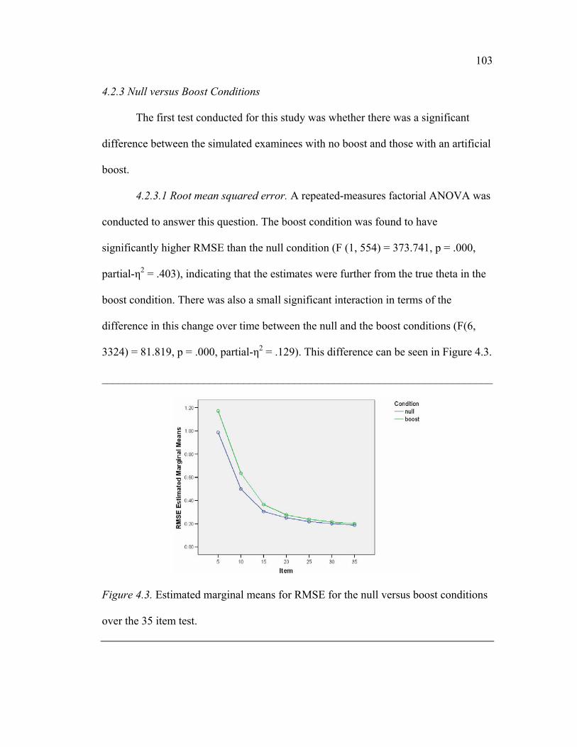
103 4.2.3 Null versus Boost Conditions

The first test conducted for this study was whether there was a significant

difference between the simulated examinees with no boost and those with an artificial

boost.

4.2.3.1 Root mean squared error. A repeated-measures factorial ANOVA was

conducted to answer this question. The boost condition was found to have

significantly higher RMSE than the null condition (F (1, 554) = 373.741, p = .000,

partial-η2 = .403), indicating that the estimates were further from the true theta in the

boost condition. There was also a small significant interaction in terms of the

difference in this change over time between the null and the boost conditions (F(6,

3324) = 81.819, p = .000, partial-η2 = .129). This difference can be seen in Figure 4.3.

_____________________________________________________________________

Figure 4.3. Estimated marginal means for RMSE for the null versus boost conditions

over the 35 item test.

104 4.2.3.2 Bias. The first test conducted for this study was whether there was a

significant difference between the simulated examinees with no boost and those with

an artificial boost. A repeated-measures factorial ANOVA was conducted. A

significant difference was found between the null and boost conditions in bias (F(1,

553) = 530.016, p = .000, partial-η2 = .489). There was a significant interaction of

time with the null and boost conditions (F(6, 3318) = 65.121, p = .000, partial-η2 =

.105). As can be seen in Figure 4.4, the null conditions started out with negative bias

compared to a large amount of positive bias for the boost conditions. By the tenth

item, both the null and boost conditions had positive bias, however, the boost

conditions consistently had significantly more positive bias than the null conditions.

This is important to note, because it suggests that examinees with a boost will have a

consistent positive error in their score estimates in comparison to those without the

boost.

105 _____________________________________________________________________

Figure 4.4. Estimated marginal means for the bias between the null and boost

conditions.

4.2.3.3 Standard deviation. The first test conducted for each independent

variable was whether there was a significant difference between the simulated

examinees with no boost and those with an artificial boost. A repeated-measures

factorial ANOVA was conducted. A large, significant difference was found between

these two groups in SD (F(1, 554) = 1970.239, p = .000, partial-η2 = .781). There was

also a significant interaction between reduction in SD over time and the null versus

boost condition variable (F(6, 3324) = 145.560, p = .000, partial-η2 = .208). As can be

seen in Figure 4.5, a large portion of the RMSE found earlier is apparent in the SD.

As well, the boost conditions consistently had a higher standard deviation than the

null conditions.

106 _____________________________________________________________________

Figure 4.5. Estimated marginal means for differences in standard deviation between

null and boost conditions.

4.2.4 Condition Type

The first independent variable of interest was type of starting rule used for the

computerized adaptive test. As stated above, there were four types of starting rules

varied: 1) RANDOM, i.e., the first item selected randomly with difficulty level close

or equal to zero (b = 0, -.5 to .5, or -1.0 to 1.0); 2) FIXED, i.e., a fixed set size for the

first five items (set size = 10, 20, or 30); 3) SHRINKING, i.e., a shrinking set size for

the first five items (set size = 10 to 2 or 20 to 4); and 4) LINEAR, i.e., a linear fixed

five-item test (difficulty level = easy, easy-to-medium, or medium).

4.2.4.1 Root mean squared error. A significant difference was found in

overall RMSE due to condition type for the conditions (F(3, 554) = 264.464, p = .000,

107 partial-η2 = .589). There was a very small significant interaction between condition

type and null versus boost (NULLBOOST) conditions (F(3, 554) = 8.331, p = .000,

partial-η2 = .043). Also, a significant interaction in terms of the change over time of

RMSE due to condition type was found for the conditions (F(18, 3324) = 132.861, p

= .000, partial-η2 = .418). This significant effect was also found to interact

significantly with the null and boost conditions (F(18, 3324) = 4.661, p = .000,

partial-η2 = .025).

Through post hoc comparisons it was found that the linear fixed test resulted

in significantly more RMSE than all three other condition types. Figure 4.6a and 4.6b

show that RMSE was greater for the linear fixed test until the twenty-fifth item at

which point the amount of RMSE was virtually the same for all condition types. Also,

comparing Figure 4.6a to 4.6b elucidates the sources of the interaction: it can be seen

that the LINEAR test type resulted in more RMSE than the other test types, and the

boost conditions resulted in more RMSE at the earlier items than did the null

conditions.

108 _____________________________________________________________________

Figure 4.6a. Estimated marginal means for the root mean squared error for each null

condition type for items over the test.

Figure 4.6b. Estimated total root mean squared error for each boost condition type

for items over the test.

109 In closer examination of the different versions of the condition types, no

significant differences were found between the first three condition types for the

conditions. However, a large significant difference was found between the linear

fixed test condition types (F(2, 132) = 436.831, p = .000, partial-η2 = .869). This

difference did not interact with the NULLBOOST variable. That is, the null and boost

conditions showed the same pattern of differences between the LINEAR starting

rules. Through post hoc comparisons, it was found that all three LINEAR starting

rules were significantly different from each other. The easy test resulted in

significantly more RMSE than the medium test (MD = .079, SED = .005, p = .000),

and the medium test resulted in significantly more RMSE than the hard test (MD =

.056, SED = .005, p = .000). These differences can be seen in Figures 4.7a and 4.7b.

Figure 4.7a. Estimated marginal means for the RMSE at each item interval for the

linear test null conditions.

110 _____________________________________________________________________

Figure 4.7b. Estimated marginal means for the RMSE at each item interval for the

linear test boost conditions.

_____________________________________________________________________

4.2.4.2 Bias. A significant difference in bias was found due to starting rule

condition type (F(3, 553) = 336.168, p = .000, partial-η2 = .646). A small significant

difference between null and boost conditions in bias due condition type was found

(F(3, 553) = 10.903, p = .000, partial-η2 = .056). A significant difference in change of

bias over time was found due to condition type (F(18, 3318) = 312.918, p = .000,

partial-η2 = .629). A very small, significant interaction between change of bias over

time due to condition type was also found between the null and boost conditions

(F(18, 3318) = 3.203, p = .000, partial-η2 = .017). Overall, the amount of bias was

more dramatic for the boost conditions than the null conditions, especially for Items 5

and 10.

111 Through post hoc comparisons it was found that the linear fixed test condition

resulted in significantly less bias than all other condition types. This can be seen in

Figures 4.8a and 4.8b. However, the amount of bias becomes almost equal to zero for

all condition types after Item 5.

Figure 4.8a. Estimated marginal means for bias between condition types for the null

conditions.

112 _____________________________________________________________________

Figure 4.8b. Estimated marginal means for bias between condition types for the boost

conditions.

In examining possible differences due to the versions of each of the condition

types, no significant differences were found between the versions of the first three

starting rule condition types. However, significant differences were found between

the linear fixed test conditions (F(2, 132) = 404.317, p = .000, partial-η2 = .860).

Through post hoc comparisons it was found that all three linear fixed tests conditions

were significantly different from each other. The easy test resulted in significantly

more negative bias than the easy-to-medium test (MD = -.075, SED = .009, p = .000)

and the medium test (MD = -.215, SED = .008, p = .000). The easy-to-medium test

resulted in significantly more negative bias than the medium test (MD = -.139, SED =

.009, p = .000). As can be seen in Figures 4.9a and 4.9b, this difference only exists

113 _____________________________________________________________________

Figure 4.9a. Estimated marginal means for bias between linear fixed test conditions

for null conditions.

Figure 4.9b. Estimated marginal means for bias between linear fixed test conditions

for boost conditions.

_____________________________________________________________________

114 at Item 5—linear fixed test with average difficulty level items (medium linear test

condition) resulted in less bias than the other two types. The easy test resulted in the

most bias. Bias begins to converge between these condition types within the null and

boost conditions around Item 10. However, at Item 10, the boost conditions had

slightly higher positive bias than the null conditions. Both the null and boost

conditions had virtually zero bias after Item 10.

4.2.4.3 Standard deviation. A significant difference was found between the

four types of conditions for starting rules (F(3, 554) = 113.692, p = .000, partial-η2 =

.381). A small, significant interaction was found between the condition types and the

null versus boost condition variable (F(3, 554) = 11.147, p = .000, partial-η2 = .057).

A large, significant interaction was also found between the change of SD over time

and the type of condition (F(18, 3324) = 736.995, p = .000, partial-η2 = .800). Finally,

a significant interaction between change over time and condition type and the null

versus boost condition variable was found (F(18, 1608) = 6.307, p = .000, partial-η2 =

.033). Overall, the amount of standard deviation is greater for the boost conditions

than the null conditions.

Through post hoc comparisons it was found that over the entire test, the linear

fixed test starting condition resulted in significantly lower SD than the other condition

types. However, in looking at Figures 4.10a and 4.10b, it can be seen that this result is

misleading. At the fifth item, the linear fixed test has significantly lower SD. At the

tenth item, the linear fixed test has significantly higher SD. Beginning around the

115 twenty-fifth item, the SD of the linear fixed test begins to converge with the other

starting conditions. This is true for both the null and boost conditions.

_____________________________________________________________________

Figure 4.10a. Estimated marginal means for standard deviation between condition

types for null conditions.

_____________________________________________________________________

116 _____________________________________________________________________

Figure 4.10b. Estimated marginal means for standard deviation between condition

types for boost conditions.

The repeated-measures, factorial ANOVA was conducted within each starting

condition type to look for differences between each version of the starting rule

condition. No significant differences were found between the versions of the starting

rules including administering a first item with difficulty level equal or close to zero

(RANDOM), a fixed set size (FIXED), or a shrinking set size (SHRINKING).

However, a significant difference was found between the three types of linear fixed

tests for the null conditions (F(2, 132) = 41.999, p = .000, partial-η2 = .389).

Through a post hoc comparison of these linear test types for the null

conditions it was found that all three test levels were significantly different from each

other. Figure 4.11a shows that at Item 5, the medium level test has significantly more

117 SD than the other two. However, at Item 10, the easy test resulted in more SD with

the easy-to-medium and medium tests having similar amounts of SD. At Items 15 and

20, the easy test still has slightly more SD and then converges with the other two

around Item 25. As can be seen in Figure 4.11b, the SD is higher for the medium

difficulty test at Item 5, then lower at Item 10. Finally, the SD becomes very similar

for all tests beginning at the fifteenth item. However, there is slightly more SD in the

medium difficulty test after the twenty-fifth item.

_____________________________________________________________________

Figure 4.11a. Estimated marginal means for standard deviation between linear test

types for null conditions.

_____________________________________________________________________

118 _____________________________________________________________________

Figure 4.11b. Estimated marginal means for standard deviation between linear test

types for boost conditions.

4.2.5 Item Pool Size

As discussed previously, three item pool sizes (ni = 100, 500, and 1000) were

examined for possible differences in RMSE, bias and standard deviation of the theta

estimate at different points in the test.

4.2.5.1 Root mean squared deviation. There was a very small significant main

effect of pool size (F( 2, 554) = 11.200, p = .000, partial-η2 = .039). There was a

marginally significant interaction between the null versus boost conditions variable

and item pool size (F(2, 554) = 3.464, p = .032, partial-η2 = .012). The RMSE was

higher at Items 5 and 10 for the boost conditions than for the null conditions.

119

Through post hoc comparisons it was found that the largest item pool (ni =

1000) resulted in significantly less RMSE than the medium item pool (ni = 500) (MD

= -.012, SED = .004, p = .002) and the small item pool (ni = 100) (MD = -.019, SED =

.004, p = .000). Also, there was a significant interaction between change over time

and the item pool sizes (F(12, 3324) = 23.186, p = .000, partial-η2 = .077). This

difference is apparent in Figures 4.12a and 4.12b which show that after the 15th item,

the 100-item pool results in significantly more RMSE than the other two pool sizes.

Also, it should be noted that for the null conditions, there is less RMSE earlier in the

test than for the boost conditions. After the 15th item, this difference is no longer

noticeable.

Figure 4.12a. Estimated marginal means for RMSE for the item pool size for the null

conditions.

_____________________________________________________________________

120 _____________________________________________________________________

Figure 4.12b. Estimated marginal means for RMSE for the item pool size for the

boost conditions.

4.2.5.2 Bias. Item pool size was varied to examine possible differences in

error of theta estimation due to having enough items. As outlined in above, three

variants of item pool size were examined: 100, 500, and 1000 items. No significant

differences were found due to pool size.

4.2.5.3 Standard deviation. Item pool size was varied to examine possible

differences in error of theta estimation due to having enough items. Three variants of

item pool size were examined: 100, 500, and 1000 items. A significant difference

between item pool sizes was found (F(2, 554) = 156.856, p = .000, partial-η2 = .362).

This difference was also found to significantly interact with the null and boost

121 conditions variable (F(2, 554) = 25.892, p = .000, partial-η2 = .085). As with the

overall differences in SD found, the null conditions resulted in less SD than the boost

conditions. Also, a small, significant interaction between reduction of SD over time

and item pool size was found (F(12, 3324) = 26.010, p = .000, partial-η2 = .086). This

change over time in SD was found to slightly interact with the null and boost

conditions variable (F(12, 3324) = 4.055, p = .000, partial-η2 = .014). Overall, the

amount of standard deviation was greater for the boost conditions.

Through post hoc comparisons it was found that all three pool sizes resulted in

significantly different levels of SD for the null conditions. It can be seen in Figure

4.13a that for the null conditions the medium sized item pool resulted in more SD for

the first 15 items, and the smallest item pool resulted in more SD for the remainder of

the test. This same pattern can be seen in Figure 4.13b for the boost conditions,

however, the amount of SD earlier in the test is larger for these conditions in

comparison to the null conditions.

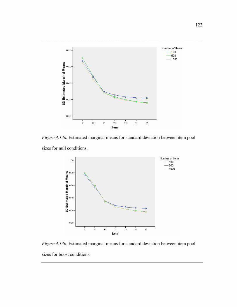
122 _____________________________________________________________________

Figure 4.13a. Estimated marginal means for standard deviation between item pool

sizes for null conditions.

Figure 4.13b. Estimated marginal means for standard deviation between item pool

sizes for boost conditions.

123 4.2.6 Discrimination Parameter Levels

To examine differences in the error of the estimation of theta value due to the

discriminating power of an item, three variants for the a-parameter were used: 1.0,

1.5, and 2.0.

4.2.6.1 Root mean squared error. The discriminating power of the item was

examined for its effect on the amount of RMSE in the theta estimate throughout the

test. A significant difference in RMSE was found due to the discrimination parameter

(F(2, 554) = 804.373, p = .000, partial-η2 = .744). There was no significant

differences interaction between the null versus boost condition variable and the

discrimination parameters. However, a small significant interaction was found

between change over time of the RMSE differing and the discrimination parameter

levels (F(12, 3324) = 9.131, p = .000, partial-η2 = .032). The differences found

between discrimination parameter levels is greater during the middle part of the test

than at the beginning and end of the test.

Through post hoc comparisons it was found that all three parameter levels were

significantly different from each other. As seen in Figures 4.14a and 4.14b,

significantly less RMSE resulted from larger discrimination parameters. Also, in

comparing these two figures, it can be seen that the null conditions had less RMSE

overall when compared to the boost conditions regardless of the level of

discrimination.

124 _____________________________________________________________________

Figure 4.14a. Estimated marginal means for RMSE between discriminating

parameters for the null conditions.

Figure 4.14b. Estimated marginal means for RMSE between discriminating

parameters for the boost conditions.

125

4.2.6.2 Bias. A very small, significant difference was found between levels of

the discrimination parameters (F(2, 553) = 15.243, p = .000, partial-η2 = .052). Also,

there was a very small significant interaction between the amount of reduction over

time in bias and the discriminating power of the items (F(12, 3318) = 10.119, p =

.000, partial-η2 = .035). The differences due to discriminating power were much

greater at Item 5 than the rest of the items.

Post hoc comparisons were conducted to find where these differences existed.

All three levels of discrimination were significantly different from each other. As can

be seen in Figures 4.15a and 4.15b, larger discrimination parameters resulted in

significantly lower bias. For the null conditions, estimates at Item 5 were much lower

than the true estimate for discrimination levels of 1.5 and 2.0. At Item 10, all three

levels resulted in average estimates slightly higher than the true theta estimate. After

Item 15, the differences between the estimates and the true thetas were virtually equal

to zero. For the boost conditions, average bias was never negative. Lower

discrimination parameters resulted in higher biases. At Item 10, these biases

converged. They continued to decrease over the length of the test, reaching an

apparent asymptote around a positive bias of .05.

126 _____________________________________________________________________

Figure 4.15a. Estimated marginal means for bias between discrimination parameter

levels for null conditions.

Figure 4.15b. Estimated marginal means for bias between discrimination parameter

levels for boost conditions.

127

4.2.6.3 Standard deviation. A large, significant difference in SD due to

discriminating ability of the items was found (F(2, 554) = 7695.878, p = .000, partial-

η2 = .965). A very small, significant interaction between the SD due to discrimination

level and the null and boost conditions variable was found (F(2, 554) = 6.915, p =

.001, partial-η2 = .024). Also, a significant interaction between change in SD over

time and discriminating ability of the items was found (F(12, 3324) = 149.059, p =

.000, partial-η2 = .350). This change was also found to significantly interact with the

null and boost conditions variable (F(12, 3324) = 3.437, p = .000, partial-η2 = .012).

Overall, the amount of standard deviation was greater for the boost conditions than

for the null conditions.

Through post hoc comparisons it was found that all three discrimination levels

were significantly different from each other. As can be seen in Figures 4.16a and

4.16b, the less discriminating an item, the more SD there is associated with the

resulting theta estimate at any point in the test. As with the other independent

variables, the amount of SD was greater for the boost conditions than for the null

conditions. This is consistent with the design of the boost conditions.

128 _____________________________________________________________________


discrimination parameter levels for null conditions.


discrimination parameter levels for boost conditions.

129 4.2.7 Guessing Parameter Levels

Analyses were conducted to examine differences in RMSE due to three

different levels of the guessing parameter (c = 0.0, 0.1, and 0.2).

4.2.7.1 Root mean squared error. Different guessing parameters resulted in

significantly different amounts of RMSE (F(2, 554) = 306.434, p = .000, partial-η2 =

.525). These differences were found to be consistent for both the null and boost

conditions; there was no interaction between the null versus boost condition variable

and the guessing parameter variable. However, a small but significant interaction was

found between change in RMSE over time and guessing parameter levels (F(12,

3324) = 30.291, p = .000, partial-η2 = .099). Differences in RMSE due to guessing

parameter levels were greater during the first half of the test. Those differences grew

smaller later in the test.

Through post hoc comparisons it was found that all three values of the

guessing parameter were significantly different from each other. Figures 4.17a and

4.17b show that the larger guessing parameters resulted in significantly more RMSE.

Also, in comparing these two figures, it can be seen that the null conditions had less

RMSE overall when compared to the boost conditions regardless of the level of the

guessing parameter.

130

Figure 4.17a. Estimated marginal means for the RMSE between guessing parameters


Figure 4.17b. Estimated marginal means for the RMSE between guessing parameters

for the boost conditions.

131

4.2.7.2 Bias. A very small, significant difference was found in bias due to

magnitude of the guessing parameter (F(2, 553) = 12.276, p = .000, partial-η2 = .043).

A very small, significant interaction between change over time and guessing

parameter level was also found (F(12, 3318) = 3.102, p = .000, partial-η2 = .011).

Differences in bias due to guessing level were greater at Items 5 and 10 than the rest

of the test.

Post hoc comparisons were conducted to see where these differences existed.

The largest discrimination parameter (c = .20) resulted in significantly higher bias

levels than the middle level (c = .10, MD = .016, SED = .006, p = .005) and the lowest

level (c = .00, MD = .028, SED = .006, p = .000). As can be seen in Figures 4.18a and

4.18b, similar differences existed for the guessing parameters as those found for the

discrimination parameter. For the null conditions (Figure 4.18a), all three levels of the

guessing parameter resulted in negative bias (that is, lower estimates of theta when

compared to the true theta value) at Item 5. At Item 10, these biases became slightly

positive. After Item 15, these biases leveled out around zero. For the boost conditions

(Figure 4.18b), the bias was very positive for the first ten items. Bias began to drop

over the subsequent items and began to level out around .05 during the last 10 items

or so.

132

Figure 4.18a. Estimated marginal means for bias between guessing parameter levels

for null conditions.

Figure 4.18b. Estimated marginal means for bias between guessing parameter levels

for boost conditions.

133

4.2.7.3 Standard deviation. A significant difference in SD due to the guessing

parameter was found (F(2, 554) = 1983.091, p = .000, partial-η2 = .877). This

difference was consistent between the null and boost conditions, that is, there was no

significant interaction between guessing parameter and the NULLBOOST variable.

However, a significant interaction between the change in SD over time and the size of

the guessing parameter was found (F(12, 3324) = 88.191, p = .000, partial-η2 = .241).

This difference was found to slightly interact with the null and boost conditions

variable (F(12, 3324) = 4.230, p = .000, partial-η2 = .015). Overall, the amount of

standard deviation was slightly greater for the boost conditions than the null

conditions.

Through post hoc comparisons it was found that all parameter levels were

significantly different from each other. As can be seen in Figures 4.19a and 4.19b, the

higher guessing parameters resulted in a higher level of SD. For both the null and

boost conditions, the SD levels out around .20. However, for the first half of the test,

consistent with the design of the study, the SD is higher for the boost conditions than


134 _____________________________________________________________________

Figure 4.19a. Estimated marginal means for standard deviation between guessing

parameter levels for null conditions.

Figure 4.19b. Estimated marginal means for standard deviation between guessing

parameter levels for boost conditions.

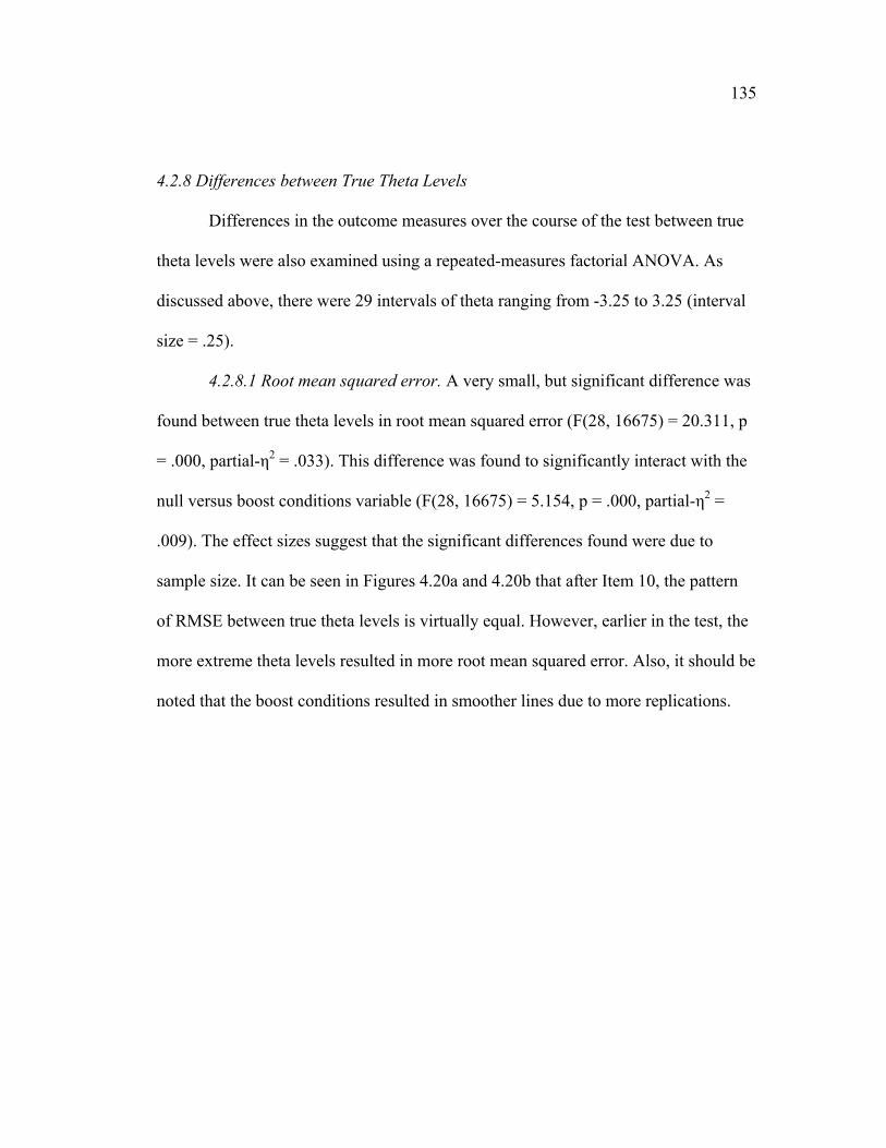
135

4.2.8 Differences between True Theta Levels

Differences in the outcome measures over the course of the test between true

theta levels were also examined using a repeated-measures factorial ANOVA. As

discussed above, there were 29 intervals of theta ranging from -3.25 to 3.25 (interval

size = .25).

4.2.8.1 Root mean squared error. A very small, but significant difference was

found between true theta levels in root mean squared error (F(28, 16675) = 20.311, p

= .000, partial-η2 = .033). This difference was found to significantly interact with the

null versus boost conditions variable (F(28, 16675) = 5.154, p = .000, partial-η2 =

.009). The effect sizes suggest that the significant differences found were due to

sample size. It can be seen in Figures 4.20a and 4.20b that after Item 10, the pattern

of RMSE between true theta levels is virtually equal. However, earlier in the test, the

more extreme theta levels resulted in more root mean squared error. Also, it should be

noted that the boost conditions resulted in smoother lines due to more replications.

136 _____________________________________________________________________

Figure 4.20a. Estimated marginal means for root mean squared error for each true

theta level across the test for the null conditions.

Figure 4.20b. Estimated marginal means for root mean squared error for each true

theta level across the test for the boost conditions.

137 4.2.8.2 Bias. Differences in bias over the course of the test between true theta

levels were also examined using a repeated-measures factorial ANOVA. A small,

significant difference was found between true theta levels in amount of bias (F(28,

16675) = 120.319, p = .000, partial-η2 = .169). A slightly significant interaction was

also found between true theta levels and the null versus boost conditions variable

(F(28, 16675) = 6.959, p = .000, partial-η2 = .012). The effect sizes suggest that the

differences found were due to sample size rather than the main effects. It can be seen

in Figures 4.21a and 4.21b that at Item 5, for both the null and boost conditions, there

was regression to the mean in terms of bias. That is, lower theta levels were biased in

a positive direction, and higher theta levels were biased in a negative direction. By

Item 10, all bias was in the positive direction. By Item 35, there were no noticeable

differences in amount of bias between the theta levels. It should also be noted that the

amount of bias for the boost conditions is consistently greater than that of the null

conditions. Also, it should be noted that the boost conditions resulted in smoother

lines due to more replications.

138

Figure 4.21a. Estimated marginal means for bias throughout the test for each true

theta level for the null conditions.

Figure 4.21b. Estimated marginal means for bias throughout the test for each true

theta level for the boost conditions.

139

4.2.8.3 Standard deviation. A very small, but significant difference was found

between true theta levels in squared deviation (F(28, 16675) = 24.562, p = .000,

partial-η2 = .040). This difference was found to significantly interact with the null

versus boost conditions variable (F(28, 16675) = 6.294, p = .000, partial-η2 = .011).

Overall, the standard deviation across theta levels is greater for the boost conditions

than it is for the null conditions. The effect sizes suggest that the significant

differences found were due to sample size. It can be seen in Figures 4.22a and 4.22b

that for both the null and boost conditions, there is less standard deviation for the

greater theta levels early in the test. At the tenth item, standard deviation becomes

virtually equal across theta levels. Also, it should be noted that the boost conditions

resulted in smoother lines due to more replications.

These results are discussed in more detail in the next section.

140

Figure 4.22a. Estimated marginal means for squared deviation throughout the test for

each true theta level for the null conditions.

Figure 4.22b. Estimated marginal means for squared deviation throughout the test for

each true theta level for the boost conditions.

_____________________________________________________________________

141

4.3 Discussion

In this study, possible differences in stability of latent trait estimate due to

varying testing parameters were examined to determine the impact of an artificial

theta boost for the first 10 items of an exam. Four testing parameters were varied: the

starting rule, the size of the item pool, the discriminating power of the items, and the

guessing parameter of the items. The patterns of differences within most of these

testing parameters were found to be slightly different between the null and the boost

conditions. Prior to discussing these testing parameters, the differences between the

null and boost conditions are discussed.

As described in Section 4.2.1, on average, the final theta estimates for the

boost conditions was about .05 points above the true theta value. As discussed later, it

can be seen that this difference reflects the systematic variability (bias) between the

boost and null conditions. These results imply that by the end of a CAT, the estimated

theta is slightly increased by the artificial boost at the beginning of the test. The boost

also impacted the stability of the latent trait estimates. Also, the general pattern of this

instability was regression toward an average theta level. That is, examinees with

negative theta levels were given much higher estimates for their ability level, while

those with very positive theta levels were estimated as much lower. The closer to an

average theta level (around zero), the less difference there was between the estimated

values and the true values. After the tenth item, the boost in estimated theta level was

pretty stable, but small. This suggests that this difference might not be worth

worrying about in practice. However, the actual effect of this boost might need to be

142 taken into account depending on the scale of the actual test used. Inferential tests are

now discussed in terms of the three outcome measures.

One important finding to discuss is that the boost conditions resulted in

significantly greater total variability (RMSE) than did the null conditions. This effect

arose from both systematic variability (bias) and random variability (SD). However,

the larger impact on the RMSE found was due to the random variability. Because the

boost was randomly varied across replications, it logically follows that this set of

conditions would have more random variability than the null set with no variation in

boost (i.e., all boosts were equal to zero). Bias is an average measure of the difference

between the estimated theta and the true theta. The difference in this measure of bias

suggests that boost and null conditions differed in the average disparity between the

estimated theta and the true theta by the amount suggested by the descriptive

statistics. Also, the pattern of differences due to starting conditions differed only

slightly between both the null and boost sets of conditions. The effect size was small

enough to suggest that the significant differences found were a function of the large

sample sizes.

For all measures of variability, the only starting rule condition that resulted in

significantly more variability were the linear fixed test conditions. Within these linear

test condition types, all three were significantly different from each other. The

medium level difficulty test always resulted from the least amount of variability. This

evidence of possible differences in test outcomes when using small fixed tests (also

known as testlets) has been addressed before (Wainer & Kiely, 1987). For all other

143 conditions, the stability of the test over time was the same. This suggests that the

starting rule does not affect the outcome of a computer adaptive test. By the twentieth

item of the test, the variability measure converged on the same value across all

conditions. Also, it should be noted that bias was close to zero after the fifteenth item;

most of the RMSE was due to random variability (SD) after the fifteenth item. These

results suggest that choosing a linear fixed test that would be too easy for the majority

of the population could result in less stable estimates earlier in the test. The main

instability is due to systematic variability after the first five items. Overall, these

findings suggest that any of the starting rules tested in this study will result in the

same outcome measure of theta after about the twentieth item.

The second independent variable in this study was the size of the item pool.

The findings of this study suggest that early on, a smaller item pool resulted in more

stable estimates, but as that pool gets smaller due to items being removed, the theta

estimates become less stable. This is probably due to a lack of items that give

maximum information at an estimated theta level after many of the items have been

removed. There was no evidence to suggest any stability differences between larger

item pool sizes. These findings give support for the argument for large item pools

when developing a computerized adaptive test (e.g., Embretson & Reise, 2000).

These differences were only apparent for the RMSE and SD measures. There were no

differences in bias (systematic variability) due to item pool sizes. It should also be

mentioned that these patterns were the same for both null and boost conditions. Thus,

144 estimates that might be affected by an artificial boost will not differ from those

without a boost due to item pool sizes.

The third independent variable of interest was the discrimination parameter of

the items. Three variants were tested (a = 1.0, 1.5, or 2.0). As would be expected, the

more discriminating items resulted in more stable estimates of theta. The

discrimination parameter gives the ability of an item to differentiate examinees with

close estimates of ability. It would logically follow that estimates based on more

discriminating items would result in more accurate estimates. Early adaptive testing

research found evidence to suggest that more discriminating items result in more

reliable theta estimates for adaptive tests (Vale & Weiss, 1975). Urry (1974, 1975)

found the 3-PL model to be more reliable than the 1-PL model for estimating theta as

long as the discrimination parameters were at least greater than .80. Jensema (1974)

also found that reliability of a test increased with larger discrimination parameters.

These findings are similar to those by other researchers who suggest using low

discriminating items earlier in the test when there is more room for error and highly

discriminating items later in the test when the CAT is fine-tuning a score. This helps

deal with the issue of item exposure rates (Chang, 1999; Hau & Chang, 2001). The

only differences found between the null and boost conditions were in the SD (random

variability) and were very slight. These results suggest that the affect that the

discrimination parameter has on the stability of the CAT is the same for both null and

boost conditions.

145 Finally, the fourth independent variable of interest was the guessing parameter

of the item. This study showed that larger guessing parameters resulted in less stable

estimates. Similar to the logic of the discrimination parameter, this makes intuitive

sense. If there is a better chance of guessing the correct answer without the true

ability to answer correctly, then this should affect the estimate of the ability level. In

this study, strong evidence was found to support the idea that creating items with less

chance for guessing the item correctly will result in more stable estimates of theta.

Jensema (1974) found that the reliability of an adaptive test increased as the size of

the guessing parameter decreased.

This inverse relationship between the reliability or stability of an estimate and

the guessing parameter is also consistent with the findings of Bridgeman and Cline

(2004) that guessing later in the test can decrease an examinee’s score. In this study,

it was found that higher guessing parameters decreased the stability of a test at all

points in the test, which supports their findings that guessing would have a potential

to dramatically affect an examinee’s final theta estimate. These results in combination

with the findings for the discrimination parameter variable suggest that creating items

with more discriminating power and less guessing possibility is optimal for stable

theta estimates. These findings were consistent for both the null and boost conditions.

Analyses were conducted to look at possible differences in these outcome

measures at different levels of true latent trait level. Although the analyses found

significant differences on all accounts, effect sizes found suggest that the significance

found was due to the number of degrees of freedom (which are a function of the

146 number of conditions examined) used to determine the significance level.

Considering that the simulated item pool was created from a normal distribution of

difficulty parameters, this might seem counterintuitive. It could be assumed that since

there are fewer items at the more extreme levels of ability, the estimates of trait at

these later points in the test would be less stable than those at a more average ability

level. However, results from this study found evidence to suggest that this is not the

case.

Overall, evidence was found to suggest that given enough items (at least 20 to

25) the maximum likelihood estimation procedure results in stable estimates of theta

no matter the starting rule selected. This is consistent with Jensema’s (1974) findings

that the reliability of an adaptive test is directly related to the length of the test. Also,

when developing an item pool for a computerized adaptive test, care should be given

to create enough items with good discriminating power and low possibilities for

guessing. If the evidence for stability of the estimates leveling out after twenty items

is coupled with the findings of Bridgeman and Cline (2004), this would suggest that

tests with 35 items could be unnecessarily long. There is also evidence that an

artificial boost to an examinee’s ability level can affect the outcome estimate of

ability level, but whether this difference is large enough is discussed next.

The important question arising from the simulation study is whether or not

this boost has a meaningful impact on scores. To examine this, GRE subtest score and

selection ratio information was collected from The Princeton Review Complete Book

of Graduate Programs (Princeton Review, 2005). Of the 1482 graduate programs

147 outlined in this book, GRE-Quantitative, GRE-Verbal and percent accepted data were

only reported for 340 programs. The average GRE score for each subtest and other

descriptive data can be found in Table 4.2. In this table, it can be seen for the GRE-V

(M = 467, SD = 118) and GRE-Q (M = 591, SD = 148) that more selective schools

have higher average scores on both subtests.

Figures 4.23 and 4.24 superimpose the results of bias from a boost on various

cutlines for selection. The mean ability estimate obtained for each true theta level

from the null and boost conditions is plotted, along with the 67% confidence interval.

These means are then compared to the average GRE-V (Figure 4.23) and GRE-Q

(Figure 4.24) for schools at certain selection ratio levels. The whiskers for the null

conditions are noticeably longer than those for the boost conditions. Considering that

there were fewer replications for the null conditions, this should be expected.

For the GRE-V, it can be seen that at a 20% selection rate, the average GRE

score falls between the null conditions and the boost conditions. Also, at the 50-90%

selection rates, examinees in the null conditions are scoring lower than the average

score, and the examinees in the boost conditions are scoring above the average score.

Given the frequency data in Table 4.2, this would affect decisions for around 200

schools. For the GRE-Q, it can be seen that this same pattern is occurring for the 30,

50 and 100% selection rate programs. At these three selection rates, there are almost

100 schools affected by this boost difference.

While these data are based on average information, they indicate that this

boost can impact selection into graduate programs. Thus, although the boost created

148 only a small inflation in final score estimates, this slight increase could very well be

enough to enhance an applicant’s chances of acceptance at a more selective school.

Given the high priority placed on test scores in our society for admissions, licensure

and scholarship purposes, future research is necessary to support this study.

Table 4.2

Descriptive statistics for average GRE-Q and GRE-V scores for 340 graduate

programs broken down by selection ratio

Selection

Ratio N Mean SD Min. Max. 0.10 3 609.3 35.92 579 649 0.20 17 588.3 48.92 528 730 0.30 29 564.4 43.82 465 621 0.40 40 542.8 43.31 475 650 0.50 35 500.9 45.09 377 598 0.60 53 499.8 54.98 300 601 0.70 57 495.7 57.61 300 659 0.80 41 488.1 56.81 323 632 0.90 33 486.8 47.40 402 581

GRE-V

1.00 28 472.4 60.97 344 600 0.10 3 649.0 78.89 600 740 0.20 17 676.3 64.08 550 773 0.30 29 636.4 73.58 451 760 0.40 40 611.2 57.76 500 750 0.50 35 596.3 80.80 392 757 0.60 53 577.3 73.56 350 770 0.70 57 585.6 79.16 380 760 0.80 41 577.0 88.14 400 728 0.90 33 531.7 57.29 450 638

GRE-Q

1.00 28 528.9 61.57 376 614

149 _____________________________________________________________________

Figure 4.23. GRE-V scores for all true theta values compared to average GRE-V

scores corresponding to each college selection ratio.

_____________________________________________________________________

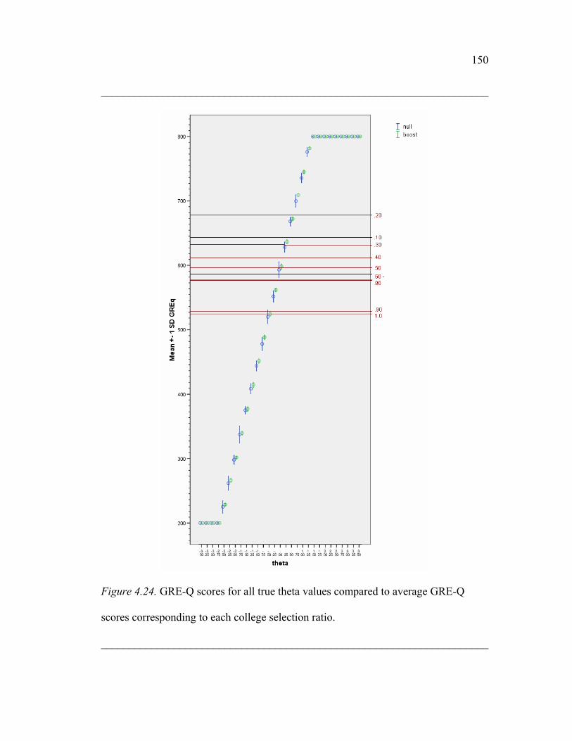
150 _____________________________________________________________________

Figure 4.24. GRE-Q scores for all true theta values compared to average GRE-Q

scores corresponding to each college selection ratio.

_____________________________________________________________________

151

5. Conclusion

In this set of studies, the impact of a test taking strategy on computerized

adaptive testing outcomes was examined. The test taking strategy of interest was one

that is taught by companies like Kaplan and Princeton Review to help “beat the test.”

Briefly, the strategy is to spend more time ensuring a correct answer on the first five

or ten items to help improve the final estimation of your ability level.

Two studies were conducted to test possible effects of this test taking strategy.

The first study looked at real world effects of knowledge of test taking strategies by

comparing three groups of examinees who differed only in the amount of instructions

they received prior to taking the same computer adaptive test. The second study

looked at the effects of an artificial boost in ability on computer adaptive test

outcomes under varying test procedure conditions.

In Study 1, differences were found in final trait estimates between conditions

that. Those examinees who were taught the test taking strategy performed better than

those without this knowledge. The examinees who performed the worst were those

who knew how the test works but were given no information on how to “beat” the

test. As discussed in Chapter 3, these differences could be due to outside examinee

factors like motivation and/or anxiety levels that might result from the knowledge, or

lack there of, of this test taking strategy. This is consistent with current literature on

test anxiety and motivation.

In Study 2, it was found that test stability patterns only differed slightly

between the two types of examinees. There was a significant difference in random

152 variability of theta estimates between the two groups of examinees, and there were

slightly significant differences in systematic variability or bias between the two

groups. This suggests that the biggest amount of differences found were due to the

variability in the initial theta boost. It was found that examinees with an artificial

boost in their ability at the beginning of the test did, on average, have an inflated final

theta estimate when compared to examinees without an artificial boost. While this

difference was significant, it was small. However, when applying these differences to

average GRE scores of graduate programs in the U.S., for schools with selection

rations especially around 50-100% this difference could result in the acceptance of

some students whose scores are not true reflections of their quantitative or verbal

reasoning ability levels.

It was also found in Study 2 that larger item pools resulted in more stable

estimates of theta. Items with higher discrimination parameters and lower guessing

parameters resulted in more stable estimates. These results are consistent with the

literature on computer adaptive testing. Also, if a test developer is interested in using

a fixed linear test to begin an adaptive test, it was found in this study that a test with

items at a more average difficulty level will result in more stable estimates of theta.

Finally, as long as tests are at least 20 items in length, the stability of the theta

estimates is virtually equal no matter the starting rule used or the presence of an

artificial boost in ability level early in the test.

Separately, these two studies lend to some interesting results. But, combining

the findings in Study 1 with those in Study 2 begins to suggest this test taking strategy

153 on average does result in inflated final ability estimates. It was found in Study 1 that

those who knew the test taking strategy had significantly better ability estimates than

those who only knew how the test works; in Study 2 that an artificial boost resulted in

significantly higher theta estimates. These results support the claim by the test review

companies that spending more time at the beginning of the test will increase your

score on the test. However, there were limitations in this set of studies that require

further attention. These limitations are discussed next.

The first of these limitations is apparent in Study 1. This study lacked the

capability to detect if the participants in the third group really followed the test taking

strategy explained to them at the beginning of the test. That is, there was no data to

see if those examinees spent more time on the first items in the test than the other

participants did. So, while there were differences found, there is no way in this study

to know for sure that these differences were due to following the test taking strategy

taught prior to the test or if they were the effects of lowered anxiety and/or higher

motivation levels.

Secondly, this study was limited to the maximum likelihood estimation

procedure. This estimation procedure is limited to examinees who answer at least one

item correctly and at least one item incorrectly. Also, this is not the only estimation

procedure in use by CAT developers and administrators. Future simulation studies

should look at other estimation procedures (e.g., EAP).

Finally, only one test taking strategy was examined in this study. In the

simulation study, this test-taking strategy was mimicked in only one way. Future

154 simulation studies should vary how this boost is applied to the true trait level. Future

studies should also attempt to isolate other human factors that could affect ability

estimates for high-stakes tests. This last point is of greatest importance given the large

role high-stakes testing plays in our society today.

155

References Arthur, Jr., W., Tubre, T. C., Paul, D. S., & Sanchez-Ku, M. L. (1999). College-

sample psychometric and normative data on a short form of the Raven

Advanced Progressive Matrices test. Journal of Psychoeducational

Assessment, 17, 354-361.

Assessment Systems Corporation. (2002). FastTEST Professional Testing System,

version 1.6.

Betz, N. E., & Weiss, D. J. (1973). An empirical study of computer-administered two-

stage ability testing (RR 73-4). Minneapolis, MN: Psychometric Methods

Program, Department of Psychology, University of Minnesota.

Betz, N. E., & Weiss, D. J. (1974). Simulation studies of two-stage ability testing (RR

74-4). Minneapolis, MN: Psychometric Methods Program, Department of

Psychology, University of Minnesota.

Betz, N. E., & Weiss, D. J. (1975). Empirical and simulation studies of flexilevel

ability testing (RR 75-3). Minneapolis, MN: Psychometric Methods Program,

Department of Psychology, University of Minnesota.

Bjorner, J. B., Kosinski, M., & Ware, Jr., J. E. (2003). Calibration of an item pool for

assessing the burden of headaches: An application of item response theory to

the Headache Impact Test (HIT). Quality of Life Research, 12, 913-933.

Bock, R. D. & Mislevy, R. J. (1982). Adaptive EAP estimation of ability in a

microcomputer environment. Applied Psychological Measurement, 6, 431-

444.

156 Bridgeman, B., & Burton, N. (2005, April). Does scoring only the hard questions on

the SAT make it fairer? Paper presented at the annual meeting of the

American Educational Research Association, Montreal.

Bridgeman, B., & Cline, F. (2004). Effects of differentially time-consuming tests on

computer-adaptive test scores. Journal of Educational Measurement, 41(2),

137-148.

Burke, H. R. (1958). Raven’s progressive matrices: A review and critical evaluation.

Journal of Genetic Psychology, 93, 199-228.

Carpenter, P. A., Just, M. A., & Shell, P. (1990). What one intelligence test measures:

A theoretical account of processing in the Raven Progressive Matrices Test.

Psychological Review, 97, 404-431.

Chang, H. H., & Ying, Z. (1999). A-stratified multistage computerized adaptive

testing. Applied Psychological Measurement, 23 (3), 211-222.

Cliff, N. (1975). Complete orders from incomplete data: Interactive ordering and

tailored testing. Psychological Bulletin, 82, 289-302.

Colvin, S. S. (1921). Intelligence and its measurement. Journal of Educational

Psychology, 12, 136-139.

Cudeck, R., McCormick, J., & Cliff, N. (1980). Implied orders tailored testing:

simulation with the Stanford-Binet. Applied Psychological Measurement, 4,

157-163.

157 Davey, T. (2005, April). An introduction to bin-structured adaptive testing. Paper

presented at the annual meeting of the National Council on Measurement in

Education, Montreal.

De Ayala, R. J. (1992). The nominal response model in computerized adaptive

testing. Applied Psychological Measurement, 16, 327-343.

Dearborne, D. F. (1921). Intelligence and its measurement: A symposium. Journal of

Educational Psychology, 12, 123-147.

Deng, H., & Ansley, T. (2003, April). To stratify or not: An investigation of CAT item

selection procedures under practical constraints. Paper presented at the

annual meeting of the National Council on Measurement in Education,

Chicago, IL.

Dodd, B. G. (1990). The effect of item selection procedure and stepsize on

computerized adaptive attitude measurement using the rating scale model.

Applied Psychological Measurement, 14, 355-366.

Elliot, E. S., & Dweck, C. S. (1988). Goals: An approach to motivation and

achievement. Journal of Personality and Social Psychology, 54 (1), 5-12.

Embretson, S. E. (1992). Measuring and validating cognitive modifiability as an

ability: A study in the spatial domain. Journal of Educational Measurement,

29 (1), 25-50.

Embretson, S. E. (1995). Working memory capacity versus general central processes

in intelligence. Intelligence, 20, 169-189.

158 Embretson, S. E. (1998). A cognitive design system approach to generating valid

tests: Application to abstract reasoning. Psychological Methods, 3(3), 380-

396.

Embretson, S. E., & Reise S. P. (2000). Item response theory for psychologists.

Mahwah, NJ: Lawrence Erlbaum Associates, Publishers

Erdfelder, E., Faul, F., & Buchner, A. (1996). GPOWER: A general power analysis

program. Behavior Research Methods, Instruments, & Computers, 28, 1-11.

Freedle, R. O. (2003). Correcting the SAT’s ethnic and social-class bias: A method

for reestimating SAT scores. Harvard Educational Review, 73(1), 1-43.

Green, B. F., Bock, R. D., Humphreys, L. G., Linn, R. L., & Reckase, M. D. (1984).

Technical guidelines for assessing computerized adaptive tests. Journal of

Educational Measurement, 21, 347-360.

Green, B. F., Jr. (1983). The promise of tailored tests. In H. Wainer & S. Messick

(Eds.), Principals of modern psychological measurement. Hillsdale, NJ:

Lawrence Earlbaum Associates.

Guilford, J. P. (1982). Cognitive psychology’s ambiguities: Some suggested

remedies. Psychological Review, 89, 48-59.

Guo, F., & Wang., L. (2003, April). Online calibration and scale stability of a CAT

program. Paper presented at the annual meeting of the National Council on

Measurement in Education, Chicago, IL.

Hambleton, R. K., Swaminathan, H., & Rogers, H. J. (1991). Fundamentals of item

response theory. Newbury Park, CA: SAGE Publications, Inc.

159 Hambleton, R. K., Zaal, J. N. & Pieters, J. P. M. (1991). Computerized adaptive

testing: Theory, application, and standards. In R. K. Hambleton & J. N. Zaal

(Eds.), Advances in educational and psychological testing: Theory and

applications. Boston, MA: Kluwer Academic Publishers.

Hansen, D. N. (1969). An investigation of computer-based science testing. In R. C.

Atkinson & H. A. Wilson (Eds.), Computer-assisted instruction: A book of

readings (pp. 209-226). New York: Academic Press.

Hau, K. T., & Chang, H. H. (2001). Item selection in computerized adaptive testing:

Should more discriminating items be used first? Journal of Educational

Measurement, 38 (3), 249-266.

Henmon, V. A. C. (1921). Intelligence and its measurement: A symposium. Journal

of Educational Psychology, 12, 195-198.

Hornke, L. F. & Habon, M. W. (1986). Rule-based item bank construction and

evaluation within the linear logistic framework. Applied Psychological

Measurement, 10(4), 369-380.

Hulin, C. L., Drasgow, F., & Parsons, C. K. (1983). Item response theory:

Application to psychological measurement. Homewood, IL: Dow-Jones Irwin.

Hunt, E. B. (1974). Quote the Raven? Nevermore. In L. W. Gregg (Ed.), Knowledge

and cognition. Hillsdale, NJ: Erlbaum. 129-158.

Jensema, C. J. (1974). An application of latent trait mental test theory. British Journal

of Mathematical Statistical Psychology, 27, 29-48.

160 Jodoin, M. G. (2005, April). A comparison of linear fixed, multi stage and adaptive

test designs. Paper presented at the annual meeting of the American

Educational Research Association, Montreal.

Kaplan. (1997). GRE: Power strategies to help you score higher, 1997-98 Ed. New

York: Kaplan Educational Centers and Simon & Schuster.

Kim, J., & McLean, J. E. (1995, April). The influences of examinee test-taking

motivation in computerized adaptive testing. Paper presented at the annual

meeting of the National Council on Measurement in Education, San

Francisco, CA.

Kingsbury, G. G. & Zara, A. R. (1991). A comparison of procedures for content-

sensitive item selection in computerized adaptive tests. Applied Measurement

in Education, 4, 241-261.

Krathwol, D. R. & Huyser, R. J. (1956). The sequential item test (SIT). American

Psychologist, 2, 419.

Larkin, K. C., & Weiss, D. J. (1974). An empirical investigation of computer-

administered pyramidal ability testing (RR 74-3). Minneapolis, MN:

Psychometric Methods Program, Department of Psychology, University of

Minnesota. (NTIS No. AD-A006 733)

Lord, F. M. (1970). Some test theory for tailored testing. In W. Holtzman (Ed.),

Computer-assisted instruction, testing, and guidance (pp. 139-183). New

York, NY: Harper & Row.

161 Lord, F. M. (1971a). The self-scoring flexilevel test. Journal of Educational

Measurement, 8, 147-151.

Lord, F. M. (1971b). A theoretical study of two-stage testing. Psychometrika, 36,

227-241.

Lord, F. M. (1977). A broad range tailored test of verbal ability. Applied

Psychological Measurement, 95-100.

Lord, F. M. (1980). Application of item response theory to practical testing problems.

Hillsdale, NJ: Lawrence Erlbaum Associates.

Lu, Y., Pitoniak, M., Rizavi, S., Way, W. D., & Steffen, M. (2003, April). Evaluating

computer adaptive testing design for the MCAT with realistic simulated data.

Paper presented at the annual meeting of the National Council on

Measurement in Education, Chicago, IL.

Luecht, R. M., & Nungester, R. (1998). Some practical examples of computer-

adaptive sequential testing. Journal of Educational Measurement, 35, 239-

249.

Maier, C. (2005). Complete Book of Graduate Programs, 2006 Ed. New York, NY:

The Princeton Review, Inc.

Martin, C. J., & Hoshaw, C. R. (2001). Policy and program management perspective.

In W. Sands, B. K. Waters, and J. R. McBride (Eds.), Computerized adaptive

testing: From inquiry to operation (pp. 11-20). Washington, DC: American

Psychological Association.

162 McBride, J. R. (2001a). Technical Perspective. In W. Sands, B. K. Waters, and J. R.

McBride (Eds.), Computerized adaptive testing: From inquiry to operation

(pp. 29-44). Washington, DC: American Psychological Association.

McBride, J. R. (2001b). Research antecedents of applied adaptive testing. In W.

Sands, B. K. Waters, and J. R. McBride (Eds.), Computerized adaptive



McBride, J. R. (2001c). The marine corps exploratory development project: 1977-

1982. In W. Sands, B. K. Waters, and J. R. McBride (Eds.), Computerized

adaptive testing: From inquiry to operation (pp. 59-67). Washington, DC:

American Psychological Association.

McBride, J. R., & Martin, J. T. (1983). Reliability and validity of adaptive ability

tests in a military setting. In D.J. Weiss (Ed.), New horizons in testing: Latent

trait theory and computerized adaptive tests (pp. 223-236). New York:

Academic Press.

McBride, J. R., & Weiss, D. J. (1976). Some properties of a Bayesian adaptive ability

testing strategy (RR 76-4). Minneapolis, MN: Psychometric Methods

Program, Department of Psychology, University of Minnesota. (NTIS No.

AD-A022 964)

163 McBride, J. R., Wetzel, C. D., & Hetter, R. D. (2001). Preliminary psychometric

research for CAT-ASVAB: Selecting an adaptive testing strategy. In W.

Sands, B. K. Waters, and J. R. McBride (Eds.), Computerized adaptive



Mead, A. D. & Drasgow, F. (1993). Equivalence of computerized and paper-and-

pencil cognitive ability tests: A meta-analysis. Psychological Bulletin, 114,

449-458.

Meijer, R. R. & Nering, M. L. (1999). Computerized adaptive testing: Overview and

introduction. Applied Psychological Measurement, 23(3), 187-194.

Moreno, K. E., Wetzel, C. D., McBride, J. R., & Weiss, D. J. (1983). Relationship

between corresponding Armed Services Vocational Aptitude Battery (ASVAB)

and computerized adaptive testing (CAT) subtests (NPRDC TR 83-27). San

Diego, CA: Navy Personnel Research and Development Center. (NTIS AD-

A131 683)

Naglieri, J. A., & Das, J. P. (1997). Das-Naglieri cognitive assessment system. Itasca,

IL: Riverside Publishing.

Neuman, G., & Baydoun, R. (1998). Computerization of paper-and-pencil tests:

When are they equivalent? Applied Psychological Measurement, 22, 71-83.

Owen, R. J. (1969). A Bayesian approach to tailored testing (RB-69-92). Princeton,

NJ: Educational Testing Services.

164 Owen, R. J. (1975). A Bayesian sequential procedure for quantal response in the

context of adaptive mental testing. Journal of the American Statistical

Association, 70, 351-356.

Pintner, R. (1927). Intelligence testing: Methods and results. New York: H. Holt and

Company.

Powers, D. E. (2001). Test anxiety and test performance: Comparing paper-based and

computer-adaptive versions of the Graduate Record Examination (GRE)

General Test. Journal of Educational Computing Research, 24 (3), 249-273.

Prabhakaran, V., Smith, J. A. L., Desmond, J. E., Glover, G. H., & Gabrieli, J. D. E.

(1997). Neural substrates of fluid reasoning: An fMRI study of neocortical

activation during performance of the Raven’s Progressive Matrices Test.

Cognitive Psychology, 33(1), 43-63.

Raven, J. (2000). The Raven’s Progressive Matrices: Change and stability over

culture and time. Cognitive Psychology, 41, 1-48.

Raven, J. C. (1962). Advanced progressive matrices Sets I and II. London: HK Lewis.

Raven, J. C., & Raven, J. (1976). Advanced progressive matrices. Oxford: Oxford

Psychologists Press.

Ree, M. J. (1977). Implementation of a model adaptive testing system at an Armed

Forces Entrance and Examining Station. In D. J. Weiss (Ed.), Proceedings of

the 1977 Computerized Adaptive Testing Conference (pp. 216-220).

Minneapolis, MN: Psychometric Methods Program, Department of

Psychology, University of Minnesota.

165 Schaeffer, G. A., Bridegman, B., Golub-Smith, M. L., Lewis, T. P., & Steffen, M.

(1998). Comparability of paper-and-pencil and computer adaptive test scores

on the GRE General Test (RR 98-38). Princeton, NJ: Educational Testing

Services. (GRE Board Professional Report No. 95-08P)

Schaeffer, G. A., Steffen, M., Golub-Smith, M. L., Mills, C. N., & Durso, R. (1995).

The introduction and comparability of the computer adaptive GRE General

Test (RR 95-20). Princeton, NJ: Educational Testing Services. (GRE Board

Professional Report No. 88-08aP)

Schoonman, W. (1989). An applied study on computerized adaptive testing.

Amsterdam: Swets & Zeitlinger B.V.

Sellman, W. S. & Arabian, J. M. (2001). Foreword. In W. Sands, B. K. Waters, and

J. R. McBride (Eds.), Computerized adaptive testing: From inquiry to

operation (pp. xv-xvii). Washington, DC: American Psychological

Association.

Shermis, M. D., & Lombard, D. (1998). Effects of computer-based test administration

on test anxiety and performance. Computers in Human Behavior, 14 (1), 111-

123.

Spearman, C. (1927). The abilities of man. New York: Macmillan.

Spray, J. A., Ackerman, T. A., Reckase, M. D., & Carlson, J. E. (1989). Effect of the

medium of item presentation on examinee performance and item

characteristics. Journal of Educational Measurement, 26, 261-271.

166 Sternberg, R. J. (1985). General intellectual ability. In R. J. Sternberg (Ed.) Human

abilities: An information processing approach. New York: W.H. Freeman

and Company, 5-29.

Still, C. (2003). The Princeton Review Crash Course for the GMAT: The Last-Minute

Guide to Scoring High, 2nd Ed (pp. 10-11). New York: Random House, Inc.

Stocking, M. L., & Swanson, L. (1993). A method for severely constrained item

selection in adaptive testing. Applied Psychological Measurement, 17, 277-

292.

Straetmans, G. J. J. M., & Eggen, T. J. H. M. (1998). Computerized adaptive testing:

What it is and how it works. Educational Technology, January-February, 45-

52.

Sympson, J. B., & Hetter, R. D. (1985). Controlling item-exposure rates in

computerized adaptive testing. Proceedings of the 27th annual meeting of the

Military Testing Association (pp. 973-977). San Diego, CA: Navy Personnel

Research and Development Center.

Terman, L. M. (1916). The measurement of intelligence. Boston, MA: Houghton

Mifflin.

Theunissen, T. J. J. M. (1986). Some applications of optimization algorithms in test

design and adaptive testing. Applied Psychological Measurement, 10, 381-

389.

167 Thissen, D., & Mislevy, R. J. (2000). Testing algorithms. In H. Wainer (Ed.),

Computer adaptive testing: A primer, 2nd Ed. (pp. 101-133). Mahwah, NJ:

Lawrence Erlbaum Associates.

Thorndike, E. L., Bregman, E. O., Cobb, M. V., & Woodyard, E. (1927). The

measurement of intelligence. New York: Bureau of Publications.

Thurstone, L. L. (1938). Primary mental abilities. Chicago: University of Chicago

Press.

Urry, V. W. (1974). Approximations to item parameters of mental test models and

their uses. Educational and Psychological Measurement, 34, 253-269.

Urry, V. W. (1977). Tailored testing: A successful application of item response

theory. Journal of Educational Measurement, 14, 181-196.

Urry, V. W. (1983). Tailored testing and practice: A basic model, normal ogive

models, and tailored testing algorithms. Washington, DC: Office of Personnel

Management.

Vale, C. D. (1975). Problem: Strategies of branching through an item pool. In D. J.

Weiss (Ed.), Computerized adaptive trait measurement: Problems and

prospects (RR 75-5). Minneapolis, MN: Psychometric Methods Program,

Department of Psychology, University of Minnesota. (AD-A018 675)

Vale, C. D., & Weiss, D. J. (1975). A simulation study of stradaptive ability testing

(RR 75-6). Minneapolis, MN: Psychometric Methods Program, Department

of Psychology, University of Minnesota. (AD-A020 961)

168 Verguts, T. & De Boeck, P. (2002). The induction of solution rules in Raven’s

Progressive Matrices Test. European Journal of Cognitive Psychology, 14(4),

521-547.

Vispoel, W. P. (1998). Psychometric characterisitcs of computer-adaptive and self-

adaptive vocabulary tests: The role of answer feedback and test anxiety.

Journal of Educational Measurement, 35 (2), 155-167.

Wainer, H. (2000). Introduction and History. In H. Wainer (Ed.), Computerized

adaptive testing: A primer, 2nd Ed (pp. 1-22). Mahwah, NJ: Lawrence

Erlbaum Associates.

Wainer, H., & Kiely, G. L. (1987). Item clusters and computerized adaptive testing: A

case for testlets. Journal of Educational Measurement, 24 (3), 185-201.

Wainer, H., & Mislevy, R. J. (2000). Item Response Theory, item calibration, and

proficiency estimation. In H. Wainer (Ed.), Computerized adaptive testing: A

primer, 2nd Ed (pp. 23-36). Mahwah, NJ: Lawrence Erlbaum Associates.

Wainer, H., & Thissen, D. (1987). Estimating ability with the wrong model. Journal

of Educational Statistics, 12, 339-368.

Ward, J., & Fitzpatrick, T. F. (1973). Characteristics of matrices items. Perceptual

and Motor Skills, 36, 987-993.

Waters, B. K. (1974). An empirical investigation of the stradaptive testing model for

the measurement of human ability. Unpublished doctoral dissertation, Florida

State University, Tallahassee, FL.

169 Weiss, D. J. (1974). The stratified adaptive computerized ability test (RR 73-3).

Minneapolis, MN: Psychometric Methods Program, Department of

Psychology, University of Minnesota. (AD 768 376)

Weiss, D. J. (1982). Improving measurement quality and efficiency with adaptive

testing. Applied Psychological Measurement, 6, 473-492.

Wise, S. L., & Kingsbury, G. G. (2000). Practical issues in developing and

maintaining a computerized adaptive testing program. Psicologica, 21, 135-

155.

170

Appendix A

Instructions for Conditions Introduction – Condition 1 – Screen 1 Thank you for agreeing to participate in this study on abstract reasoning ability. This is a computer adaptive test that measures your ability to reason on a nonverbal matrix completion task. The test you are about to take has 25 matrix completion items. Before beginning the test, you will be given examples of the rules necessary to complete all items in the test. You will also be given an example item to practice these rules before beginning the test. You will not be allowed to skip any items or return to any items you have already answered. Please click on the button below to acknowledge that you have signed and received a copy of the informed consent form with information on how to contact the researchers in this study at any point after completion of this study. Then, click "Next" in the upper, right-hand corner of the screen to move on.

171 Introduction – Condition 2 – Screen 1 Thank you for agreeing to participate in this study on abstract reasoning ability. This is a computer adaptive test that measures your ability to reason on a nonverbal matrix completion task. The test you are about to take is computer adaptive and has 25 matrix completion items. Before beginning the test, you will be given examples of the rules necessary to complete all items in the test. You will also be given an example item to practice these rules before beginning the test. A computer adaptive test "adapts" itself to test takers by selecting the next item to be presented on the basis of performance on preceding items. This means that each item you receive on the test is chosen from a large number of items and the choice is made based on whether you answered previous questions correctly or incorrectly. This also means that the items you receive may not be the same items or they may not be given to you in the same order as others taking this test. Because of the nature of this test, you will not be allowed to skip any items or return to any items you have already answered. Please click on the button below to acknowledge that you have signed and received a copy of the informed consent form with information on how to contact the researchers in this study at any point after completion of this study. Then, click "Next" in the upper, right-hand corner of the screen to move on.

172 Introduction – Condition 3 – Screen 1 Thank you for agreeing to participate in this study on abstract reasoning ability. This is a computer adaptive test that measures your ability to reason on a nonverbal matrix completion task. The test you are about to take is computer adaptive and has 25 matrix completion items. Before beginning the test, you will be given examples of the rules necessary to complete all items in the test. You will also be given an example item to practice these rules before beginning the test. A computer adaptive test "adapts" itself to test takers by selecting the next item to be presented on the basis of performance on preceding items. This means that each item you receive on the test is chosen from a large number of items and the choice is made based on whether you answered previous questions correctly or incorrectly. This also means that the items you receive may not be the same items or they may not be given to you in the same order as others taking this test. Because of the nature of this test, you will not be allowed to skip any items or return to any items you have already answered. One test taking strategy that you should keep in mind when taking this test is as follows... Because of the nature of a computer adaptive test, you will want to spend time and concentration on the first ten questions of the test. The reason for this is that a computer adaptive test relies heavily on the first ten questions in determining your score. This is because the computer knows nothing about your ability before you start the test. Because of the short length of this test, the needs to use pretty big jumps in judgment in the first ten questions and then use the remaining questions to "fine-tune" your score. Please click on the button below to acknowledge that you have signed and received a copy of the informed consent form with information on how to contact the researchers in this study at any point after completion of this study. Then, click "Next" in the upper, right-hand corner of the screen to move on.

173

174 Instructions – Screen 2 The matrix completion items you will be given throughout this test are similar the one below. There are three rows and three columns of pictures that follow particular patterns. You must first figure out the pattern then choose the correct answer (numbered 1 through 8) that fulfills this pattern to fill in the ninth spot (represented by the "?").

Please click "Next" to learn the rules necessary to complete these items.

175 Instructions – Screen 3 The first rule is known as Identity. This rule states that the same element is found across the rows and/or down the columns. As in the picture below, there is a square in every element of the first row, a triangle in every element of the second row and a circle in every element of the third row. This rule can be applied down the columns as well if there were a same attribute down every element of a column.

Please click "Next" to move on to the next rule.

176 Instructions – Screen 4 The second rule for these items is Progression. As can be seen in the example below, this rule implies a change in the attribute from the first to the third element in that row or column. For this example, the shapes get bigger as you move from left to right. This rule could consist of changes in number of shapes (e.g., one square to three squares) or shade of the shape (e.g., white to grey to black).


177 Instructions – Screen 5 The third rule for these items is Addition/Subtraction. As can be seen in the first example below, this rule results in adding the attributes in each of the first elements of each row AND column to create the third element (e.g., the horizontal line added to the vertical line creates the plus sign at the end of the first row). Or, in the second example, looking at the first column, if you take the asterisk looking element, and remove from it the diagonal lines (the second element in the column), the resulting element is the plus sign.


178 Instructions – Screen 6 The fourth rule for these items is Distribution of 3. As can be seen in the example below, each row and column contains one of three attributes that are evenly distributed over every row and column. Each row and column contains one square, one circle and one triangle.

Please click "Next" to move on to the final rule.

179 Instructions – Screen 7 The final rule for these items is Distribution of 2. As can be seen in the example below, each row and column has two elements with identical attributes and the third element consists of some contrasting attribute. For example, the first row consists of two elements with triangles and the third element contains a circle.

Please click "Next" to move on to an example item.

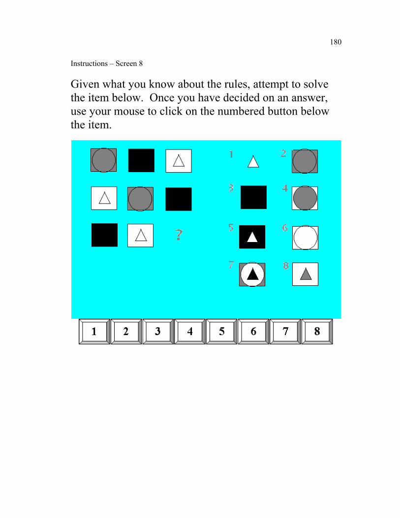
180 Instructions – Screen 8 Given what you know about the rules, attempt to solve the item below. Once you have decided on an answer, use your mouse to click on the numbered button below the item.

181 Instructions – Screen 9 If you answered 2, you are correct. Remembering the rules from earlier, we can see that the identity rule is used (a square in every row and column). As well, there are two Distribution of 3 rules in play. Each row and column has one element that's grey, one that's white and one that's black. As well, each row and column has one element containing a circle, one containing a square and one containing a triangle.

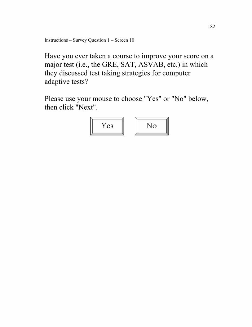
182 Instructions – Survey Question 1 – Screen 10 Have you ever taken a course to improve your score on a major test (i.e., the GRE, SAT, ASVAB, etc.) in which they discussed test taking strategies for computer adaptive tests? Please use your mouse to choose "Yes" or "No" below, then click "Next".

183 Instructions – Survey Question 1 – Screen 11 Have you ever taken a computer adaptive test before (e.g., the GRE, ASVAB, etc.)? Please use your mouse to choose "Yes" or "No" below, then click "Next".

184

Appendix B

Means (and standard deviations) for theta boosts for each level of theta

Theta Item1 Item2 Item3 Item4 Item5 Item6 Item7 Item8 Item9 Item10 -3.50 .687 .343 .229 .172 .137 .114 .098 .086 .076 .069

(.650) (.325) (.217) (.163) (.130) (.108) (.093) (.081) (.072) (.065) -3.25 .675 .337 .225 .169 .135 .112 .096 .084 .075 .068

(.618) (.309) (.206) (.154) (.124) (.103) (.088) (.077) (.069) (.062) -3.00 .670 .335 .223 .167 .134 .112 .096 .084 .074 .067

(.577) (.289) (.192) (.144) (.115) (.096) (.082) (.072) (.064) (.058) -2.75 .690 .345 .230 .173 .138 .115 .099 .086 .077 .069

(.653) (.326) (.218) (.163) (.131) (.109) (.093) (.082) (.073) (.065) -2.50 .653 .327 .218 .163 .131 .109 .093 .082 .073 .065

(.708) (.354) (.236) (.177) (.142) (.118) (.101) (.089) (.079) (.071) -2.25 .682 .341 .227 .170 .136 .114 .097 .085 .076 .068

(.614) (.307) (.205) (.154) (.123) (.102) (.088) (.077) (.068) (.061) -2.00 .667 .334 .222 .167 .134 .111 .095 .083 .074 .067

(.676) (.338) (.225) (.169) (.135) (.113) (.097) (.085) (.075) (.068) -1.75 .675 .338 .225 .169 .135 .113 .096 .084 .075 .068

(.627) (.313) (.209) (.157) (.125) (.104) (.090) (.078) (.070) (.063) -1.50 .697 .349 .232 .174 .139 .116 .100 .087 .078 .070

(.602) (.301) (.201) (.150) (.120) (.100) (.086) (.075) (.067) (.060) -1.25 .667 .334 .222 .167 .133 .111 .095 .083 .074 .067

(.580) (.290) (.193) (.145) (.116) (.097) (.083) (.072) (.064) (.058) -1.00 .662 .331 .221 .165 .132 .110 .095 .083 .074 .066

(.633) (.317) (.211) (.158) (.127) (.106) (.090) (.079) (.070) (.063) -.75 .693 .347 .231 .173 .139 .116 .099 .087 .077 .069

(.703) (.352) (.234) (.176) (.141) (.117) (.100) (.088) (.078) (.070) -.50 .705 .352 .235 .176 .141 .118 .101 .088 .078 .071

(.716) (.358) (.239) (.179) (.143) (.119) (.102) (.089) (.080) (.072) -.25 .668 .334 .223 .167 .134 .111 .096 .084 .074 .067

(.629) (.314) (.210) (.157) (.126) (.105) (.090) (.079) (.070) (.063) .00 .691 .345 .230 .173 .138 .115 .099 .086 .077 .069

(.622) (.311) (.207) (.156) (.124) (.104) (.089) (.078) (.069) (.062) .25 .720 .360 .240 .180 .144 .120 .103 .090 .080 .072

(.665) (.332) (.222) (.166) (.133) (.111) (.095) (.083) (.074) (.066) .50 .675 .338 .225 .169 .135 .113 .096 .084 .075 .068

(.584) (.292) (.195) (.146) (.117) (.097) (.083) (.073) (.065) (.058) .75 .729 .364 .243 .182 .146 .121 .104 .091 .081 .073

(.699) (.350) (.233) (.175) (.140) (.117) (.100) (.087) (.078) (.070)

185

Appendix B (continued)

Means (and standard deviations) for theta boosts for each level of theta

Theta Item1 Item2 Item3 Item4 Item5 Item6 Item7 Item8 Item9 Item10 1.00 .670 .335 .223 .168 .134 .112 .096 .084 .075 .067

(.611) (.305) (.204) (.153) (.122) (.102) (.087) (.076) (.068) (.061) 1.25 .689 .344 .230 .172 .138 .115 .098 .086 .077 .069

(.667) (.333) (.222) (.167) (.133) (.111) (.095) (.083) (.074) (.067) 1.50 .701 .351 .234 .175 .140 .117 .100 .088 .078 .070

(.702) (.351) (.234) (.176) (.140) (.117) (.100) (.088) (.078) (.070) 1.75 .636 .318 .212 .159 .127 .106 .091 .080 .071 .064

(.574) (.287) (.191) (.144) (.115) (.096) (.082) (.072) (.064) (.057) 2.00 .661 .331 .220 .165 .132 .110 .095 .083 .074 .066

(.635) (.317) (.212) (.159) (.127) (.106) (.091) (.079) (.071) (.063) 2.25 .708 .354 .236 .177 .142 .118 .101 .089 .079 .071

(.671) (.336) (.224) (.168) (.134) (.112) (.096) (.084) (.075) (.067) 2.50 .663 .332 .221 .166 .133 .111 .095 .083 .074 .066

(.635) (.317) (.212) (.159) (.127) (.106) (.091) (.079) (.071) (.063) 2.75 .696 .348 .232 .174 .139 .116 .100 .087 .077 .070

(.670) (.335) (.223) (.168) (.134) (.112) (.096) (.084) (.074) (.067) 3.00 .694 .347 .231 .173 .139 .116 .099 .087 .077 .069

(.624) (.312) (.208) (.156) (.125) (.104) (.089) (.078) (.069) (.062) 3.25 .690 .345 .230 .172 .138 .115 .099 .086 .077 .069

(.745) (.372) (.248) (.186) (.149) (.124) (.106) (.093) (.083) (.074) 3.50 .671 .336 .224 .168 .134 .112 .096 .084 .075 .067

(.610) (.305) (.203) (.152) (.122) (.102) (.087) (.076) (.068) (.061)

186

Appendix C Means (and standard deviations) for the theta estimate at seven points throughout the

test within each true theta level

Theta Item5 Item10 Item15 Item20 Item25 Item30 Item35 -3.50 -2.678 -3.222 -3.379 -3.417 -3.431 -3.437 -3.444

(.354) (.075) (.020) (.020) (.023) (.025) (.028) -3.25 -2.515 -3.003 -3.134 -3.172 -3.189 -3.197 -3.202

(.292) (.054) (.016) (.016) (.018) (.021) (.022) -3.00 -2.307 -2.746 -2.881 -2.921 -2.938 -2.946 -2.953

(.251) (.049) (.0167) (.014) (.015) (.016) (.019) -2.75 -2.075 -2.498 -2.631 -2.668 -2.681 -2.691 -2.698

(.221) (.048) (.017) (.013) (.012) (.013) (.014) -2.50 -1.888 -2.264 -2.387 -2.419 -2.435 -2.443 -2.449

(.201) (.045) (.019) (.016) (.014) (.014) (.015) -2.25 -1.665 -1.990 -2.117 -2.160 -2.176 -2.188 -2.194

(.172) (.042) (.023) (.019) (.017) (.017) (.019) -2.00 -1.463 -1.763 -1.884 -1.924 -1.939 -1.949 -1.954

(.171) (.039) (.022) (.016) (.013) (.014) (.015) -1.75 -1.245 -1.512 -1.627 -1.666 -1.685 -1.694 -1.699

(.184) (.041) (.024) (.019) (.017) (.018) (.019) -1.50 -.980 -1.244 -1.374 -1.411 -1.429 -1.439 -1.446

(.227) (.042) (.020) (.020) (.021) (.022) (.023) -1.25 -.761 -.993 -1.119 -1.158 -1.177 -1.187 -1.193

(.261) (.046) (.029) (.028) (.026) (.026) (.027) -1.00 -.561 -.753 -.865 -.908 -.928 -.938 -.943

(.299) (.045) (.031) (.025) (.023) (.024) (.025) -.75 -.320 -.500 -.621 -.659 -.677 -.687 -.693

(.363) (.054) (.032) (.028) (.025) (.024) (.024) -.50 -.100 -.267 -.386 -.420 -.437 -.445 -.451

(.423) (.047) (.036) (.029) (.025) (.025) (.025) -.25 .114 -.003 -.128 -.166 -.182 -.190 -.197

(.489) (.051) (.028) (.023) (.021) (.020) (.020) .00 .341 .256 .123 .082 .065 .055 .049

(.562) (.053) (.036) (.031) (.028) (.027) (.026) .25 .570 .508 .383 .345 .327 .315 .308

(.648) (.052) (.031) (.025) (.023) (.022) (.023) .50 .755 .744 .620 .582 .566 .555 .549

(.720) (.047) (.032) (.025) (.023) (.021) (.021)

187

Appendix C (continued)

Means (and standard deviations) for the theta estimate at seven points throughout the

test within each true theta level

Theta Item5 Item10 Item15 Item20 Item25 Item30 Item35 .75 .977 1.002 .867 .830 .813 .805 .798

(.811) (.056) (.030) (.023) (.021) (.019) (.017) 1.00 1.139 1.222 1.103 1.070 1.053 1.046 1.041

(.881) (.058) (.034) (.025) (.021) (.019) (.018) 1.25 1.334 1.482 1.354 1.317 1.300 1.293 1.288

(.962) (.053) (.031) (.022) (.018) (.016) (.015) 1.50 1.534 1.722 1.602 1.565 1.551 1.542 1.538

(1.049) (.056) (.023) (.019) (.015) (.015) (.013) 1.75 1.713 1.957 1.849 1.816 1.801 1.792 1.787

(1.133) (.059) (.027) (.021) (.017) (.014) (.013) 2.00 1.908 2.219 2.106 2.071 2.055 2.046 2.040

(1.226) (.070) (.023) (.017) (.013) (.011) (.010) 2.25 2.114 2.447 2.343 2.313 2.298 2.288 2.284

(1.327) (.063) (.032) (.026) (.019) (.017) (.015) 2.50 2.248 2.663 2.584 2.557 2.543 2.535 2.530

(1.395) (.071) (.023) (.015) (.014) (.011) (.010) 2.75 2.421 2.906 2.844 2.814 2.797 2.789 2.784

(1.490) (.105) (.028) (.020) (.016) (.015) (.015) 3.00 2.517 3.140 3.090 3.066 3.051 3.042 3.036

(1.550) (.121) (.032) (.022) (.018) (.016) (.015) 3.25 2.638 3.360 3.338 3.315 3.299 3.292 3.286

(1.618) (.122) (.033) (.022) (.019) (.017) (.018) 3.50 2.760 3.555 3.582 3.566 3.555 3.547 3.541

(1.688) (.172) (.035) (.026) (.022) (.020) (.020)

188

Appendix D Estimated theta value mean and 95% confidence interval for each true theta for boost

conditions

True theta = -3.25

-3.21

-3.11

-3.01

-2.91

-2.81

-2.71

-2.61

-2.51

MeanLower BoundUpper Bound

Mean -2.5154 -3.0029 -3.1337 -3.1717 -3.1885 -3.1967 -3.2019

Lower Bound -2.5492 -3.0092 -3.1356 -3.1736 -3.1905 -3.1991 -3.2045

Upper Bound -2.4815 -2.9966 -3.1318 -3.1699 -3.1864 -3.1943 -3.1992

item5 item10 item15 item20 item25 item30 item35

Thet

a

189

True theta = -3.00

-2.97

-2.87

-2.77

-2.67

-2.57

-2.47

-2.37

-2.27


Mean -2.3067 -2.7459 -2.8811 -2.9205 -2.9384 -2.9464 -2.9526

Lower Bound -2.3358 -2.7516 -2.8831 -2.9221 -2.9401 -2.9483 -2.9548

Upper Bound -2.2776 -2.7403 -2.8792 -2.9189 -2.9367 -2.9445 -2.9504


Thet

a

190

True theta = -2.75

-2.7

-2.6

-2.5

-2.4

-2.3

-2.2

-2.1


Mean -2.0748 -2.4981 -2.6307 -2.6675 -2.681 -2.6907 -2.6979

Lower Bound -2.1005 -2.5036 -2.6327 -2.6691 -2.6824 -2.6922 -2.6995

Upper Bound -2.0492 -2.4925 -2.6287 -2.6659 -2.6796 -2.6893 -2.6962


Thet

a

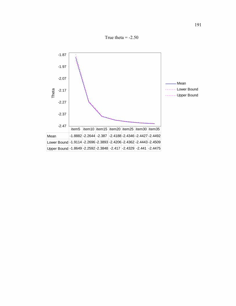
191

True theta = -2.50

-2.47

-2.37

-2.27

-2.17

-2.07

-1.97

-1.87


Mean -1.8882 -2.2644 -2.387 -2.4188 -2.4346 -2.4427 -2.4492

Lower Bound -1.9114 -2.2696 -2.3893 -2.4206 -2.4362 -2.4443 -2.4509

Upper Bound -1.8649 -2.2592 -2.3848 -2.417 -2.4329 -2.441 -2.4475


Thet

a

192

True theta = -2.25

-2.21

-2.11

-2.01

-1.91

-1.81

-1.71


Mean -1.6649 -1.9902 -2.1173 -2.1595 -2.1763 -2.1877 -2.1939

Lower Bound -1.6849 -1.9951 -2.1199 -2.1616 -2.1783 -2.1897 -2.1961

Upper Bound -1.6449 -1.9854 -2.1146 -2.1573 -2.1744 -2.1857 -2.1918


Thet

a

193

True theta = -2.00

-1.97

-1.87

-1.77

-1.67

-1.57

-1.47


Mean -1.4633 -1.7631 -1.8837 -1.9235 -1.9394 -1.949 -1.9544

Lower Bound -1.4831 -1.7676 -1.8862 -1.9253 -1.9409 -1.9506 -1.9562

Upper Bound -1.4435 -1.7585 -1.8811 -1.9217 -1.938 -1.9474 -1.9527


Thet

a

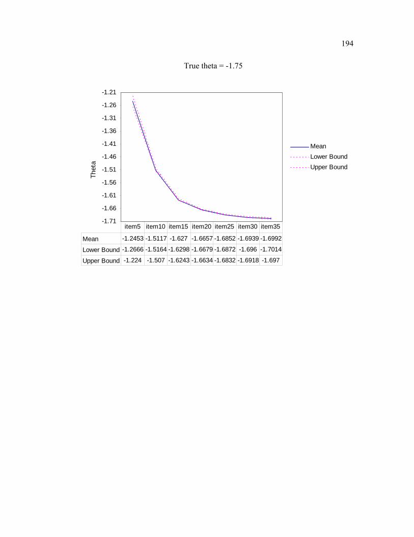
194

True theta = -1.75

-1.71

-1.66

-1.61

-1.56

-1.51

-1.46

-1.41

-1.36

-1.31

-1.26

-1.21


Mean -1.2453 -1.5117 -1.627 -1.6657 -1.6852 -1.6939 -1.6992

Lower Bound -1.2666 -1.5164 -1.6298 -1.6679 -1.6872 -1.696 -1.7014

Upper Bound -1.224 -1.507 -1.6243 -1.6634 -1.6832 -1.6918 -1.697


Thet

a

195

True theta = -1.50

-1.455

-1.355

-1.255

-1.155

-1.055

-0.955


Mean -0.9803 -1.2435 -1.3737 -1.411 -1.429 -1.4385 -1.4462

Lower Bound -1.0066 -1.2484 -1.3761 -1.4134 -1.4315 -1.441 -1.4489

Upper Bound -0.954 -1.2386 -1.3714 -1.4087 -1.4265 -1.436 -1.4435


Thet

a

196

True theta = -1.25

-1.2

-1.15

-1.1

-1.05

-1

-0.95

-0.9

-0.85

-0.8

-0.75


Mean -0.7606 -0.9928 -1.1186 -1.1584 -1.1766 -1.1866 -1.1932

Lower Bound -0.7908 -0.9982 -1.122 -1.1617 -1.1796 -1.1897 -1.1964

Upper Bound -0.7304 -0.9874 -1.1152 -1.1552 -1.1735 -1.1836 -1.19


Thet

a

197

True theta = -1.00

-0.95

-0.9

-0.85

-0.8

-0.75

-0.7

-0.65

-0.6

-0.55


Mean -0.561 -0.7533 -0.8651 -0.9082 -0.928 -0.9375 -0.9432

Lower Bound -0.5956 -0.7585 -0.8687 -0.9111 -0.9307 -0.9404 -0.9461

Upper Bound -0.5263 -0.748 -0.8614 -0.9052 -0.9253 -0.9347 -0.9402


Thet

a

198

True theta = -0.75

-0.71

-0.66

-0.61

-0.56

-0.51

-0.46

-0.41

-0.36

-0.31


Mean -0.3196 -0.5004 -0.6208 -0.6593 -0.6767 -0.6865 -0.6932

Lower Bound -0.3617 -0.5066 -0.6245 -0.6626 -0.6795 -0.6892 -0.696

Upper Bound -0.2775 -0.4942 -0.6171 -0.656 -0.6738 -0.6838 -0.6904


Thet

a

199

True theta = -0.50

-0.46

-0.41

-0.36

-0.31

-0.26

-0.21

-0.16

-0.11

-0.06


Mean -0.0998 -0.2669 -0.3857 -0.4202 -0.4365 -0.445 -0.4509

Lower Bound -0.1489 -0.2724 -0.3899 -0.4236 -0.4394 -0.4479 -0.4538

Upper Bound -0.0508 -0.2614 -0.3815 -0.4168 -0.4336 -0.442 -0.4479


Thet

a

200

True theta = -0.25

-0.205

-0.155

-0.105

-0.055

-0.005

0.045

0.095

0.145


Mean 0.1141 -0.0028 -0.1282 -0.1662 -0.1816 -0.1901 -0.1966

Lower Bound 0.0574 -0.0088 -0.1315 -0.1689 -0.184 -0.1924 -0.1989

Upper Bound 0.1708 0.0031 -0.125 -0.1635 -0.1792 -0.1878 -0.1943


Thet

a

201

True theta = 0.00

0.04

0.09

0.14

0.19

0.24

0.29

0.34

0.39


Mean 0.3407 0.2559 0.1233 0.0817 0.0646 0.0552 0.0486

Lower Bound 0.2756 0.2498 0.1191 0.0782 0.0613 0.0521 0.0456

Upper Bound 0.4059 0.262 0.1275 0.0853 0.0678 0.0583 0.0516


Thet

a

202

True theta = 0.25

0.3

0.35

0.4

0.45

0.5

0.55

0.6

0.65


Mean 0.5704 0.5083 0.383 0.345 0.3265 0.315 0.3081

Lower Bound 0.4952 0.5023 0.3793 0.3421 0.3239 0.3124 0.3055

Upper Bound 0.6456 0.5143 0.3866 0.348 0.3291 0.3176 0.3107


Thet

a

203

True theta = 0.50

0.54

0.59

0.64

0.69

0.74

0.79

0.84


Mean 0.7553 0.7435 0.62 0.5822 0.5664 0.5548 0.5485

Lower Bound 0.6719 0.7381 0.6163 0.5793 0.5638 0.5524 0.546

Upper Bound 0.8388 0.749 0.6238 0.5851 0.5691 0.5573 0.5509


Thet

a

204

True theta = 0.75

0.79

0.84

0.89

0.94

0.99

1.04


Mean 0.9766 1.0015 0.8674 0.8298 0.8134 0.8048 0.7983

Lower Bound 0.8826 0.995 0.8638 0.8271 0.811 0.8026 0.7963

Upper Bound 1.0706 1.008 0.8709 0.8325 0.8158 0.807 0.8003


Thet

a

205

True theta = 1.00

1.03

1.08

1.13

1.18

1.23


Mean 1.1392 1.2223 1.103 1.0704 1.0533 1.0455 1.0405

Lower Bound 1.037 1.2156 1.0991 1.0676 1.0509 1.0433 1.0384

Upper Bound 1.2414 1.229 1.1069 1.0733 1.0558 1.0477 1.0426


Thet

a

206

True theta = 1.25

1.22

1.27

1.32

1.37

1.42

1.47


Mean 1.3339 1.4818 1.3535 1.3165 1.3002 1.2931 1.2877

Lower Bound 1.2223 1.4756 1.35 1.3139 1.2981 1.2913 1.286

Upper Bound 1.4454 1.4879 1.3571 1.3191 1.3023 1.295 1.2894


Thet

a

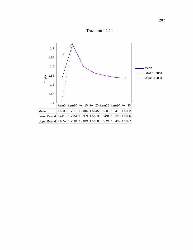
207

True theta = 1.50

1.4

1.45

1.5

1.55

1.6

1.65

1.7


Mean 1.5335 1.7219 1.6016 1.5645 1.5508 1.5415 1.5382

Lower Bound 1.4118 1.7154 1.5989 1.5623 1.5491 1.5398 1.5366

Upper Bound 1.6552 1.7284 1.6043 1.5668 1.5524 1.5432 1.5397


Thet

a

208

True theta = 1.75

1.575

1.625

1.675

1.725

1.775

1.825

1.875

1.925


Mean 1.7132 1.9567 1.8491 1.8162 1.8011 1.7921 1.7868

Lower Bound 1.5818 1.9499 1.846 1.8138 1.7992 1.7905 1.7853

Upper Bound 1.8447 1.9635 1.8523 1.8186 1.8031 1.7937 1.7883


Thet

a

209

True theta = 2.00

1.76

1.81

1.86

1.91

1.96

2.01

2.06

2.11

2.16

2.21


Mean 1.9076 2.2193 2.1055 2.0707 2.0554 2.046 2.0396

Lower Bound 1.7655 2.2111 2.1029 2.0687 2.0538 2.0447 2.0384

Upper Bound 2.0498 2.2274 2.1082 2.0727 2.0569 2.0472 2.0408


Thet

a

210

True theta = 2.25

1.955

2.005

2.055

2.105

2.155

2.205

2.255

2.305

2.355

2.405

2.455


Mean 2.1138 2.4472 2.3432 2.3131 2.2981 2.2884 2.2838

Lower Bound 1.9598 2.4399 2.3395 2.3101 2.2959 2.2865 2.2821

Upper Bound 2.2678 2.4545 2.3469 2.3161 2.3002 2.2903 2.2856


Thet

a

211

True theta = 2.50

2.08

2.18

2.28

2.38

2.48

2.58

2.68


Mean 2.2483 2.6626 2.584 2.5566 2.5428 2.5348 2.5298

Lower Bound 2.0865 2.6544 2.5813 2.5549 2.5412 2.5335 2.5286

Upper Bound 2.4101 2.6708 2.5867 2.5584 2.5444 2.5361 2.531


Thet

a

212

True theta = 2.75

2.245

2.345

2.445

2.545

2.645

2.745

2.845


Mean 2.4213 2.9064 2.8439 2.8135 2.7972 2.7892 2.7839

Lower Bound 2.2485 2.8942 2.8407 2.8112 2.7953 2.7874 2.7822

Upper Bound 2.5942 2.9187 2.8472 2.8159 2.7991 2.791 2.7856


Thet

a

213

True theta = 3.00

2.335

2.435

2.535

2.635

2.735

2.835

2.935

3.035

3.135


Mean 2.5172 3.14 3.0895 3.0656 3.0506 3.0419 3.0364

Lower Bound 2.3374 3.126 3.0858 3.063 3.0485 3.04 3.0346

Upper Bound 2.6969 3.154 3.0932 3.0682 3.0527 3.0437 3.0382


Thet

a

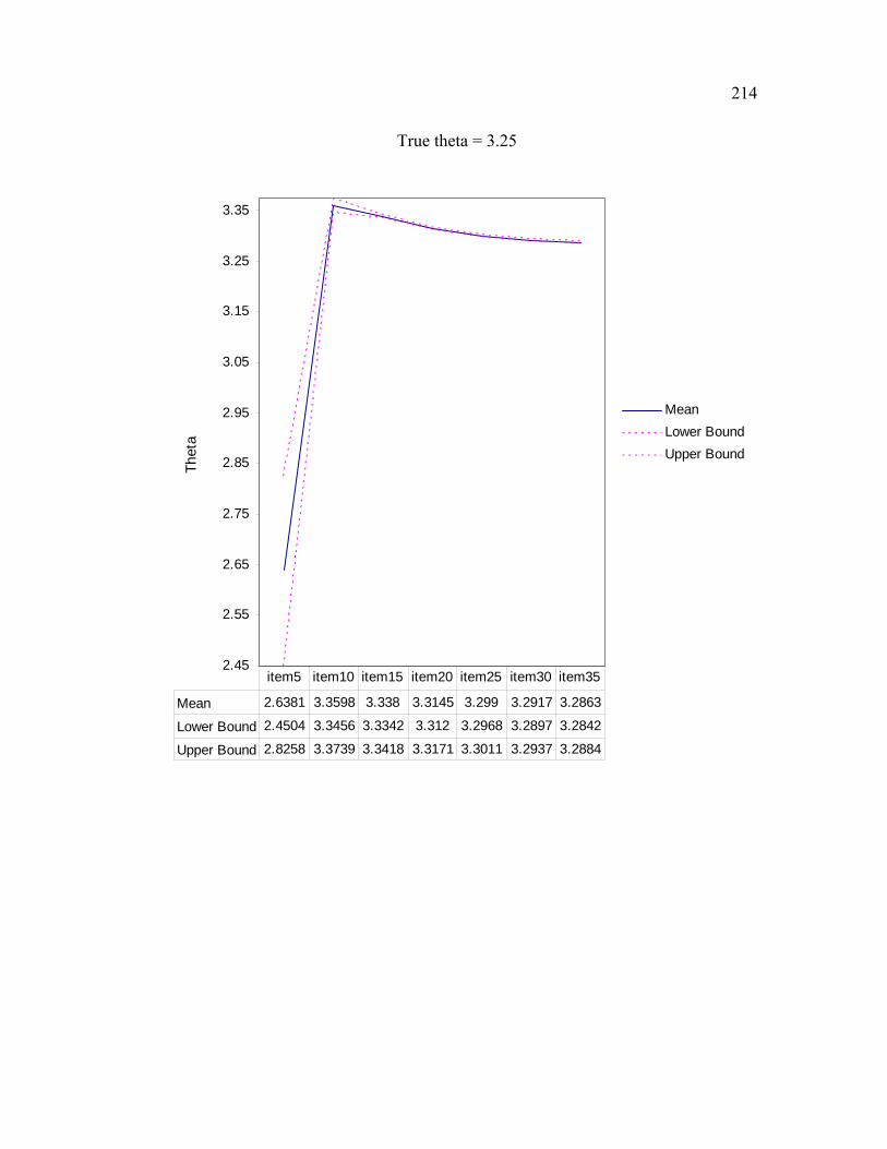
214

True theta = 3.25

2.45

2.55

2.65

2.75

2.85

2.95

3.05

3.15

3.25

3.35


Mean 2.6381 3.3598 3.338 3.3145 3.299 3.2917 3.2863

Lower Bound 2.4504 3.3456 3.3342 3.312 3.2968 3.2897 3.2842

Upper Bound 2.8258 3.3739 3.3418 3.3171 3.3011 3.2937 3.2884


Thet

a

Documents

Test Taking Strategies in Computer Adaptive Testing that