Embed Size (px)
Citation preview
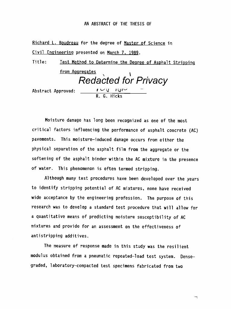
AN ABSTRACT OF THE THESIS OF
Richard L. Boudreau for the degree of Master of Science in
Civil Engineering presented on March 7, 1989.
Title: Test Method to Determine the Degree of Asphalt Stripping
from AggregatesI
Redacted for PrivacyAbstract Approved: FL'k.1 PU1"
R. G. Hicks
Moisture damage has long been recognized as one of the most
critical factors influencing the performance of asphalt concrete (AC)
pavements. This moistureinduced damage occurs from either the
physical separation of the asphalt film from the aggregate or the
softening of the asphalt binder within the AC mixture in the presence
of water. This phenomenon is often termed stripping.
Although many test procedures have been developed over the years
to identify stripping potential of AC mixtures, none have received
wide acceptance by the engineering profession. The purpose of this
research was to develop a standard test procedure that will allow for
a quantitative means of predicting moisture susceptibility of AC
mixtures and provide for an assessment on the effectiveness of
antistripping additives.
The measure of response made in this study was the resilient
modulus obtained from a pneumatic repeatedload test system. Dense
graded, laboratorycompacted test specimens fabricated from two

aggregate sources in the state of Oregon were evaluated in this
research.
The test procedure and specimen preparation developed was
implemented with a saturation and freezethaw moisture condition
cycling. Results indicate that the procedure can significantly
differentiate between a proven stripping aggregate and a proven non
stripping aggregate. The comparison can be made following full
saturation plus one freezethaw cycle. Results also indicate that
caution must be used when comparing mixes of different air void
contents. The results of the procedure developed appear to over
predict moisture susceptibility of low air void groups (<6.5%) and
under predict moisture susceptibilty of high air void groups (>8.5%).
The procedure also has a strong potential to assess the effectiveness
of antistripping additives, although some of the additives evaluated
in this study generally did not improve the mixtures sensitivity to
moisture damage.

Test Method to Determine theDegree of Asphalt Stripping from Aggregates
by
Richard L. Boudreau
A THESIS
submitted to
Oregon State University
in partial fulfillment ofthe requirements for the
degree of
Master of Science
Completed March 7, 1989
Commencement June 1990

APPROVED: \\
Redacted for PrivacyProfessor of Civil Engineering in Charge of Major
Redacted for PrivacyHeii_jp.fibepartmeniWcTv1)6WeeTT
111111111111111k
Redacted for PrivacyDean of Graduge School
Date Thesis is Presented March 7.1989
Typed by researcher for Richard L. Boudreau

1
ACKNOWLEDGEMENTS
The author wishes to express his sincere gratitude to his project
advisor, Dr. Gary Hicks, for his guidance, patience, encouragement, and
criticism over the long haul.
A special thank you is extended to Bud Furber, Andy Brickman, and
Todd Scholz for technical input and needed support.
The author is also grateful to Professor David Faulkenberry, Dr.
Chris Bell, and Dr. Bob Leichti for their active participation on the
graduate committee.
Joanne Heddlesten deserves special recognition for her excellent
organization of tables included in this document.
Finally, I must thank my conscience, my strong will to achieve, my
patience, my wife Mimi, who possesses more of these characteristics
than me. She should be as proud of this thesis as I.

11
TABLE OF CONTENTS
Page
1 INTRODUCTION 1
1.1 Problem Statement 1
1.2 Study Objective 3
1.3 Scope of Study 4
2 MATERIALS AND TEST METHODS 6
2.1 Diametral Modulus Testing Apparatus 8
2.1.1 The Load System 8
2.1.2 Testing Accessories 11
2.1.3 Recording Device 14
2.2 Test Procedures 14
2.2.1 Repeated-Load Diametral Test 14
2.2.2 Moisture Conditioning 21
2.3 Materials 26
2.3.1 Parametric Study 26
2.3.2 Compaction Study 28
2.3.3 Factorial Study 33
3 PARAMETRIC STUDY 39
3.1 Experimental Design 39
3.1.1 Material Variables 41
3.1.2 Procedural Variables 43
3.2 Specimen Preparation 45
3.3 Test Results 47
3.4 Analysis of Results 52
3.5 Conclusions and Recommendations 60
4 COMPACTION STUDY 61
4.1 Experimental Design 61
4.2 Mixing and Curing 62
4.3 Compaction Method 65
4.3.1 Static Compaction (ASTM D1074) 654.3.2 Marshall Compaction (ASTM D1559) 66
4.3.3 Kneading Compaction (ASTM D1561) 69

111
TABLE OF CONTENTS
Page
4.3.4 Gyratory-shear Compaction (ASTM D4013) 71
4.4 Analysis and Results 74
4.5 Conclusions and Recommendations 80
5 PRIMARY FACTORIAL STUDY 81
5.1 Objectives 81
5.2 Experimental Design 83
5.2.1 Materials 85
5.2.2 Specimen Preparation 88
5.3 Test Results 89
5.4 Discussion of Results 102
5.5 Conclusions and Recommendations 108
6 CONCLUSIONS AND FINAL RECOMMENDATIONS 115
6.1 Conclusions 116
6.2 Recommendations 119
7 BIBLIOGRAPHY 122

iv
LIST OF FIGURES
Number Page
1.1 Schematic of Stripping Process 2
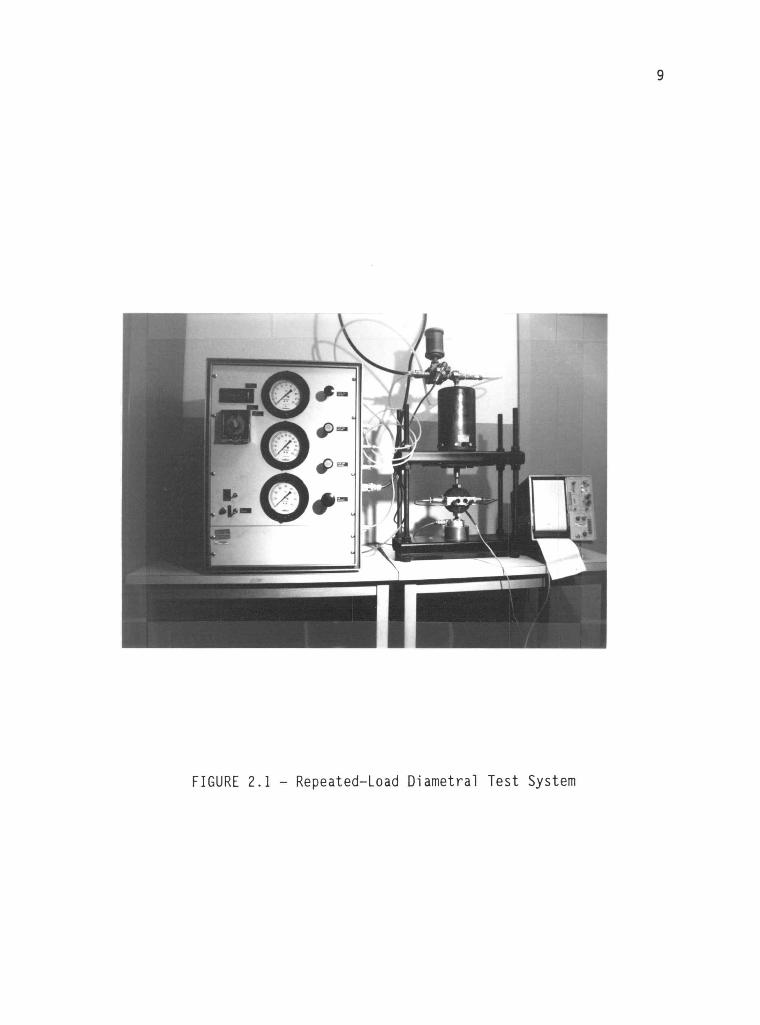
2.1 Repeated-Load Diametral Test System 9
2.2 Load Frame with Loading Components 10
2.3 Air Control Cabinet 12
2.4 Test Specimen with Diametral Yoke and Loading Ram . . 13
2.5 Signal Conditioning Device 15
2.6 Typical Load-Deflection Response Trace 18
2.7 Temperature Control Cabinet 20
2.8 Moisture Conditioning Process 22
2.9 Vacuum Saturation Apparatus 24
4.1 Laboratory Program Compaction Study 64
4.2 Static Compaction Equipment (ASTM D1074) 67
4.3 Marshall Compaction Equipment (ASTM D1559) 68
4.4 Kneading Compaction Equipment(ASTM D1561) 70
4.5 Gyratory-shear Compaction Equipment (ASTM D4013) 72
5.1 Laboratory Program - Factorial Study 84
5.2 IRMr vs. Condition Cycles Aggregate A 92
5.3 IRMr vs. Condition Cycles Aggregate B 93
5.4 Typical Specimen at Low Air Void ContentsFollowing 5 Freeze-thaw Cycles 109
5.5 Typical Specimen at Intermediate Air Void ContentsFollowing 5 Freeze-thaw Cycles 110
5.6 Typical Specimen at High Air Void ContentsFollowing 5 Freeze-thaw Cycles 111

LIST OF TABLES
Number Page2.1 Summary of Laboratory Procedures to Determine
Water Sensitivity of Asphalt Concrete 7
2.2 ODOT Mix Designs for Dense Graded C-mixParametric Study 27
2.3 Summary of Aggregate Properties Parametric Study . . 27
2.4 Physical Properties of AR-4000W Parametric Study andCompaction Study 29
2.5 Chemical Composition of AR-4000W Parametric Study andCompaction Study 30
2.6 Properties of Ash Grove "Kemilime" Hydrated Lime 31
2.7 ODOT Mix Designs for Dense Graded C-mix - Compactionand Factorial Studies 32
2.8 Summary of Aggregate Proprties Compaction andFactorial Studies 32
2.9 Physical Properties of AR-4000W Factorial Study . . . 35
2.10 Chemical Composition of AR-4000W Factorial Study . . 36
2.11 Properties of AC-20R Factorial Study 37
3.1 Procedural and Material Variables 40
3.2 Experimental Design ANOVA 42
3.3 Test Conditions for Parametric Study 44
3.4 Summary of Specific Gravities and Air Void ContentsParametric Study 46
3.5 Effects of Temperature on Mr Group A4 48
3.6 Effects of Load Duration on Mr Group A4 48
3.7 Effects of Load Frequency on Mr Group A4 48
3.8 Effects of Temperature on Mr Group A10 49
3.9 Effects of Load Duraton on Mr Group A10 49

vi
LIST OF TABLES
Number Page
3.10 Effects of Load Frequency on Mr - Group A10 49
3.11 Effects of Temperature on Mr Group BL4 50
3.12 Effects of Load Duration on Mr Group BL4 50
3.13 Effects of Load Frequency on Mr Group BL4 50
3.14 Effects of Temperature on Mr Group B10 51
3.15 Effects of Load Duration on Mr Group B10 51
3.16 Effects of Load Frequency on Mr Group B10 51
3.17 Summary of Analysis of Variance Instantaneous Mr . . . . 53
3.18 Summary of Analysis of Variance Total Mr 54
3.19 Mean Instantaneous M of Four Material GroupsUnder Different Levels of Settings 55
3.20 Mean Total Mr of Four Material Groups UnderDifferent Levels of Settings 55
3.21 Supplemental Temperature Study Total Mr 58
4.1 Experimental Design ANOVA Compaction Study 63
4.2 Total Mr Test Results Compaction Study 75
4.3 ANOVA for Total Mr at 40°F 76
4.4 ANOVA for Total Mr at 73°F 77
4.5 Summary of M Means, Standard Errors, andSignificant Differences at 40°F 78
5.1 Experimental Design ANOVA Primary FactorialStudy 86
5.2 Summary of Kneading Compaction Effort andAir Voids Achieved Factorial Study 90
5.3 Summary of IRMr (%) Test Results and Analysis 94
5.4 Summary of IRMr (%) Test Results and StatisticalAnalysis for Aggregate B 96

vii
LIST OF TABLES
Number Page
5.5 Summary of IRMr (%) Test Results and StatisticalAnalysis for Aggregate A 97
5.6 Summary of IRMr Results Following OneFreeze-thaw Cycle 99
5.7 Significant Differences of Treatment MeansFollowing One Freeze-thaw Conditioning Cycle 100
5.8 Air Void Content Comparison Before and AfterConditioning 106
5.9 Correction to the IRMr Due to Air Void Changes 107

TEST METHOD TO DETERMINE THEDEGREE OF ASPHALT STRIPPING FROM AGGREGATES
1 INTRODUCTION
1.1 Problem Statement
The durability of an asphalt concrete (AC) pavement depends to a
great degree on the adhesion between the asphalt cement and the
aggregate. Although construction methods, traffic, environmental
conditions and mix properties contribute to the deterioration of an AC
pavement, the presence of water or water vapor (moisture) often is one
of the most critical factors affecting the durability of asphalt
concrete mixtures (Lottman, 1982).
Water or moisture damage in AC pavements may be associated with
two mechanisms (Kennedy et al., 1983). First, aggregates generally
have a greater affinity for water than asphalt. Water can get between
the asphalt and aggregate and "strip" the asphalt film away. This
mechanism for loss of adhesion may be viewed in terms of a reduction
in the contact angle between the asphalt and aggregate surface, as
shown in Figure 1.1. The rate at which adhesion stripping takes place
is a function of temperature, type of aggregate and viscosity and
composition of the asphalt (Tyler, 1938). This theory suggests that
"bare" aggregates at the extreme may be the result of adhesion loss.
The second probable mechanism identified is the interaction of water
with the asphalt cement (or emulsification) which causes a reduction
in cohesion with a severe reduction in integrity and strength of the

2
(a) The moment at which the aggregate, with the drop of bitumen, is immersed1 in water. The contact angle is less than 90'.
(b) The water begins to remove the bitumen drop from the aggregate surfaceand the contact angle decreases.
(c) Finally, the stage is reached where the contact angle is 0' and thebitumen loses contact with the aggregate surface.
FIGURE 1.1 Schematic of the Stripping Process (after Tyler, 1938).

3
mixture (White, 1987). This type of stripping is not as visible to
the human eye as the loss of adhesion mechanism. Graf (1986) reports
that the cohesive failure theory can further be divided into two
distinctly different types of failure. The first involves a softening
of the AC in the presence of water which will lead to failure within
the asphalt film of the aggregate matix. The other involves the
softening of the AC which weakens the bond between the AC and the
aggregate, causing a seperation of the film from the aggregate.
Therefore an adhesion failure may be thought of as a combination of
cohesion loss and adhesion loss.
1.2 Study Objective
A wide variety of test procedures have been developed to predict
the moisture susceptibility of asphalt concrete pavements. Although
many of the test procedures have produced good results in localized
regions of the country, a common test procedure has not been developed
that is widely accepted by the engineering profession. This study is
concerned with the development of a standard test procedure to be used
to determine the stripping potential of a compacted AC mixture by
means of a RepeatedLoad Diametral Test System.
The overall goal of this study is to develop an improved test
method to quantify the susceptibility of an asphalt concrete mixture
to stripping which allows a quantitative assessment of the
effectiveness of antistripping additives. Specific objectives
include:

4
1. Selection of test conditions that will discriminate between
material characteristics (ie: air voids, asphalt type and
content, aggregate type, etc.) while yielding repeatable
results.
2. Selection of a laboratory compaction method that results in
a high degree of replication in air void contents and
repeatability in resilient modulus.
3. Implementation and evaluation of a moistureconditioning
process and test method that will meet the overall goals of
this study as mentioned above.
1.3 Scope of Study
A detailed discussion of the RepeatedLoad Diametral Test
equipment and procedure is presented in Chapter 2. Also presented in
Chapter 2 is a description of the materials used to prepare the
laboratory compacted specimens and the moistureconditioning process
to initiate stripping.
The Parametric Study presented in Chapter 3 is a quantitative
study of controlled laboratory compacted AC specimen subjected to a
series of variable resilient modulus test conditions. The variable
conditions include temperature, load duration and frequency, and
induced strain level desired to perform the test. The resilient
modulus at each combination of test conditions is recorded and
evaluated. The conclusions derived in this portion of the study are
intended to meet the criteria of specific objective number one listed
previously.

5
The presentation of the Compaction Study in Chapter 4 is intended
to aid in the development of sample preparation. Four methods of
compaction and two curing procedures are evaluated for specimen
consistency including air void contents and resulting resilient
modulus values. The method of compaction and curing which result in
the highest degree of repeatability will be used as the method of
compaction for the proposed improved test method.
The Factorial Study presented in Chapter 5 is a concentrated
laboratory testing effort using the testing conditions and compaction
method developed in Chapters 3 and 4. In this study, the test method
incorporates an accelerated moistureconditioning process on mixtures
containing two separate aggregate types, two asphalt types and two
antistripping agents. The results of the resilient modulus tests are
analyzed and evaluated for additive effectiveness, and the ability of
the improved test method to be sensitive to moisture damage.
Finally, the conclusions and recommendations resulting from this
study are given in Chapter 6.

6
2 MATERIALS AND TEST METHODS
A number of test methods have been developed over the years to
identify the susceptibility of an AC mixture to moisture. The number
of tests have recently increased with greater concern for stripping
and evaluation of antistripping agents. Available tests range from a
qualitative inspection of coated aggregates in a loose mixture
submerged in water at ambient or elevated temperatures to more
quantitative mechanical responses to moisture of compacted AC
mixtures. A summary of some of the available tests are listed in
Table 2.1 (after Taylor and Khosla, 1983).
This paper presents an evaluation of a repeatedload diametral
test procedure to detect the susceptibility of AC mixtures to moisture
damage. The repeatedload diametral procedure to determine the
resilient modulus (Mr) was selected over the methods briefly outlined
in Table 2.1 because the test is nondestructive. The nondestructive
nature of the test allows measurement of strength loss over repetitive
cycles of conditioning on the same sample. This will decrease the
number of samples required for testing over the destructive testing
alternatives, and variations in strength loss should only be
attributed to the conditioning of the samples, and not slight
differences in replication of samples (i.e., by testing the same sets
of sample => exact replication!).
The Mr concept provides support for the more recent acceptance
the Mr incorporated in the new AASHTO pavement design guide (AASHTO,
1986). The Mr of a compacted AC mixture is believed to be a measure of

7
TABLE 2.1 -Summary of Laboratory Procedures to Determine WaterSensitivity of Asphalt Concrete (modified after Taylor andKhosla, 1983)
Dynamic Immersion TestsNicholson TestDow or Tyler Wash Test
Technique
Static Immersion TestsASTM D-1664Lee TestHolmes Water DisplacementOberbach TestGerman U-37 Test
Boiling TestsASTM D-3625Riedel and Weber Test
Chemical Immersion TestsRiedel and Weber Test
Abrasion TestsCold Water Abrasion TestAbrasion-Displacement TestSurface Water Abrasion Test
Simulated Traffic TestsEnglish Trafficking TestsTest Tracks
Quantitative Coating Evaluation TestsDye Absorption TestMechanical Integration MethodRadioactive Isotope Tracer
Tracer-Salt with Flame PhotometerAnalysis
Light-Reflection Method
Nondestructive TestsSonic TestResilient Modulus Test
Immersion-Mechanical TestsMarshall Immersion TestMoistureVaporSusceptibilityTestWater Susceptibility TestIndirect Tension (Diametral
Compression) TestImmersion-Compression Test
ASTM D-1075 or AASHTO T-165
Miscellaneous TestsDetachment TestsBriquet Soaking TestStripping Coefficient MeasurementPeeling TestTexas Freeze-Thaw Pedestal Test

8
the elastic response of a pavement under conditions which simulate
repeated traffic loads. Therefore, the Mr has been employed in the
mechanistic design procedure for asphalt concrete pavements.
The following sections describe the equipment used to determine
the Mr of compacted AC mixtures. Also a discussion of the Mr test
procedure and the moistureconditioning process employed to initiate
stripping is presented. Lastly, presented in this chapter is a
description of the materials used to prepare laboratory test specimens
for the 1) Parametric Study, 2) Compaction Study and 3) Factorial
Study. The materials used include aggregates, asphalt and
antistripping additives.
2.1 Diametral Modulus Testing Apparatus
The Mr used to identify the stripping potential and effectiveness
of antistripping additives for this study were determined with a
RepeatedLoad Diametral Test System (ASTM, 1987a). The RepeatedLoad
System consists of three basic units: (1) the load system, (2) testing
accessories, and (3) recording devices. Each of these units are
described below.
2.1.1 The Load System
The load system is shown in Figure 2.1. It includes an air
powered testing apparatus and a control cabinet from which dynamic and
static load can be controlled. Figure 2.2 shows the electropneumatic
system used to apply loads. It consists of a Bellofram air cylinder,
a shuttle valve and a MAC valve. Operation of the MAC valve requires
9
FIGURE 2.1 RepeatedLoad Diametral Test System

10
FIGURE 2.2 Load Frame with Loading Components

11
a 110 volt power supply, a pilot air supply, and a main air supply
(100-125 psi air pressure). The Bellofram air cylinder can be
activated either by the MAC valve line or the static load line. The
shuttle valve regulates airflow to the Bellofram air cylinder and is
designed to allow the line of highest pressure to flow into the air
cylinder. Because the MAC valve is normally closed, the static load
line is connected to the Bellofram air cylinder when the MAC valve is
not activated by an electrical signal. If the MAC valve is activated,
the shuttle valve closes the static load line and opens the MAC valve
line to the Bellofram air cylinder. Static and dynamic load pressure
lines, and electrical signals to the MAC valve are monitored from the
control cabinet.
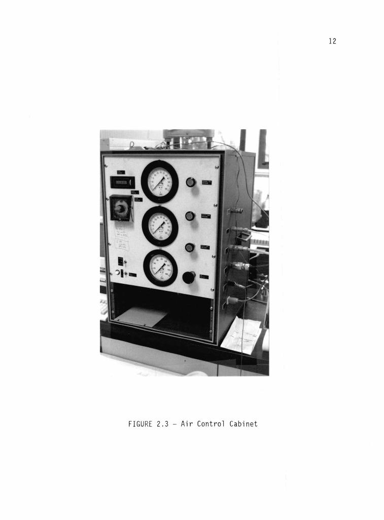
The control cabinet, shown in Figure 2.3, contains a pneumatic
system able to supply air to the Bellofram cylinder and an electrical
system designed primarily to monitor the MAC valve. Precision air
regulators and pressure gauges control the static and dynamic air
pressure lines. A dual timer controls the electrical signal to the
MAC valve (pulse interval and pulse duration) and a counter to record
the number of load pulses.
2.1.2 Testing Accessories
A diametral yoke (Figure 2.4) is required to conduct repeated
load diametral tests. The yoke is used to mount LVDT's (Sangamo
Linear Variable Differential Transformers [LVDT's], model no. AG/2.5)
which measure the horizontal deformation of cylindrical samples
subjected to dynamic vertical load. The sample horizontal deformation
12
FIGURE 2.3 Air Control Cabinet

13
LVDTGauge Head
LVDTAdjustmentKnob
DiametralYoke
Loading Ram
Diametral Attachment
Top Loading Strip
To Strip ChartRecorder
Thumb Screws
Bottom Loading Strip
Platen (Rests On,..-Load Frame Base
Plate)
FIGURE 2.4 Test Specimen with Diametral Yoke and Loading Ram

14
is measured by the LVDT's. The dynamic load is measured using a flat
load cell (Strainsert Universal Load Cell, model no. FL2.5 U2SGKT, 2.5
kip capacity).
2.1.3 Recording Device
A two channel oscillographic stripchart recorder (Figure 2.5),
with A/C carrier preamplifiers, is used for the diametral test
transducer LVDT's and the load cell. Detailed information on both the
oscillographic recorder and the A/C preamplifiers is presented in the
operating and service manuals supplied by the manufacturer (e.g.,
HewlettPackard, Gould, etc.).
2.2 Test Procedures
The following sections describe the test procedure used to
determine the Mr of compacted AC mix specimen, and the moisture
conditioning process used to simulate field moisture conditions. The
moistureconditioning process was only used for the Primary Factorial
Study presented in Chapter 5.
2.2.1 RepeatedLoad Diametral Test
The test procedure used in this study to determine the Mr was
done in accordance with ASTM D4123 (1987a). In this procedure, a
nominal 4inch diameter cylindrical specimen undergoes a repeated load
along its vertical diametral plane. The load and the horizontal
elastic deformation are measured with a calibrated signal conditioner
(i.e., a twochannel oscillographic stripchart recorder) after a

15
FIGURE 2.5 Signal Conditioning Device (Hewlett Packard 2channelStrip Chart Recorder)

16
series of preconditioning loads. The purpose of preconditioning a
specimen is to eliminate early plastic flow and achieve good contact
between the specimen and the platen. This should result in a stable
deformation readout, and typically takes 50 100 load pulses at room
temperature. Fewer preconditioning load pulses are required for low
temperature testing (less plastic), and more may be required for
higher temperatures (more plastic).
The load and deflection data obtained from an individual test is
used to calculate the Mr using equation 2.1:
Mr = P(v+0.27)/Ht (2.1)
where Mr = Resilient modulus, psi.t = specimen thickness, in.P = dynamic pulse load, lbs.H = horizontal elastic deformation, in.v = Poisson's Ratio
The tensile strain at the center of the specimen is given by:
Et = [(0.16+0.48v)/(0.27+v)] x H (2.2)
Equations 2.1 and 2.2 are supported by work done by Hadley et
al.(1970). A typical value of Poisson's ratio for asphaltic concrete
is 0.35 (Yoder and Witczak, 1975); therefore equations 2.1 and 2.2 can
be reduced to:
Mr = 0.62 (P/Ht) (2.3)
Et = 0.52H (2.4)
The testing operator can control the magnitude of the applied
pulse load by using the pulse load regulator on the front panel of the
control cabinet. By adjusting the load, the operator can target the

17
horizontal elastic deformation required to achieve a predetermined
strain level (eq 2.4). Note that the load reading and the horizontal
deformation occur simultaneously on the twochannel stripchart
recorder (Figure 2.6). The Mr test mobilizes small strains in the
specimen. Under small strains the material approaches the elastic
range of its stressstrain response (Heinicke and Vinson, 1988).
Further, it is desirable to test at small strain levels as this
condition will avoid damage to the specimen, hence making the test
nondestructive. A microstrain level of 50 150 (1 microstrain =
1x10⁻⁶ in/in) was determined to satisfy this case (ASTM, 1987a).
The horizontal displacement that the test specimen undergoes as a
result of an applied vertical load may be measured either upon load
application or release. The former measurement leads to determination
of the socalled total Mr while the latter is used to determine the so
called instantaneous Mr (ASTM, 1987a). A typical load and displacement
response trace from a 2channel stripchart recorder is shown in
Figure 2.6.
It is somewhat simpler to measure the total displacement (HT)
than it is to measure the instantaneous (HI) as the instantaneous
displacement is smaller and strain relaxation must be accounted for in
determining the measurement. The instantaneous Mr is preferred from a
theoretical viewpoint, because it represents the elastic response and
should be more sensitive to the degree adhesion (and loss of cohesion)
than is the total Mr, which is influenced by plastic strain that occurs
at load application (Kelley et al., 1986). Both measurements were
made in the Parametric Study. Results were analyzed to determine

18
1 (r NI) 5
E=."."-INEEMISEMENIIIMENEMEM=-"-=E=1-..W.IMMEMMENIMEMEffireig..2=m=
Mal=M =W-IMENE W um111 En mem umailligim
.=:L.:=nE M-MW.,
=. :IE::===iiME=E Eas.,1=We En=Effmew,UM EE =REM E:=-Ia.:=_...........siBEE==leffi=e====== emme =me=ram=fammaiswaimmin=COQ=
.525icora=EE=. E=E.= g===Eiffi ara= = = mm.I=Essal ..0.1..
m_mmumws gEnpi,I5t- (A)
MI 1111111111111 ' 1 ==E=.1=1, =
zulemE
Emni4=1=...._............
.-.--MME_.--.1rIEElmni
....i..n...= mrismEm.d-4MN IIMINNIMI11.11
moi=w--=6.==.9n.TE=E=2L:...i.m........fflia1......,.. ".". SIL.1.' MUM
1la---Em----.._...i
mi_E-massmeastanimmliti
,-- 1 ,.1=
--___#-,.----,-,e
Sample Calculation for pulse (A): Specimen thickness, t = 2.5 in.
1. Load Pen Displacement = 17 mm Load Calibration = 10 lb/mm =>Load (P)=170 lbs.
2. Instantaneous DeflectionPen Displacement = 12mm Defl. Calibration = 9 Ain/mm => HI = 108 Ain.
3. Total DeflectionPen Displacement = 15 mm Defl. Calibration = 9 Ain/mm => HT = 135 gin
Diametral Strain et = 0.52 HT = 0.52 (135 Ain) = 70.2 microstrain
Instantaneous Mr = 0.62 [P /(H1)(t)] = 0.62 [1701b/(135 x 10 6 in)(2.5 in)] = 390,370 psi
Total Mr = 0.62 [P/(HT)(t)] = 0.62 [1701b./(108 x 106 in)(2.5in)] = 312,296 psi
FIGURE 2.6 Typical LoadDeflection Response Trace

19
which measurement is most sensitive to material changes while yielding
reliable results. Because the instantaneous Mr better characterizes
the elastic response of the asphalt concrete mixture it should be used
in instances where the test data is to be used for evaluation of
structural performance of pavements.
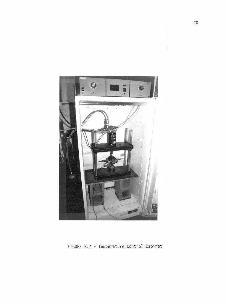
Testing temperatures of 40, 73 and 100° F were selected for Mr
testing for the Parametric Study. The range of temperatures was
selected in order to analyze the effects of temperature on the Mr as
well as to determine the testing temperature that produces repeatable
results within similar material groups. Test temperatures can be
controlled by performing the tests inside a control cabinet. A
refrigerator with temperature control was used (Figure 2.7). Test
temperatures of 55 and 73°F for derived Emodulus values from the
indirect tensile strength test were studied in the development of the
Lottman procedure. The 55°F test temperature was found to give a
stronger indication of moisture susceptibility for Emodulus ratios
(Lottman, 1982).
The advantage of the nondestructive testing is that the Mr can
be calculated from test specimen response to low strain levels. This
is significant because the same test specimen can be tested throughout
the conditioning cycles described in the following section, reducing
the number of specimens required in the moisturesusceptibility test
procedures developed by Lottman. This is also significant in the fact
that errors associated with testing socalled "replicated" groups is
minimized.
20
FIGURE 2.7 Temperature Control Cabinet

21
2.2.2 Moisture Conditioning
The laboratory specimens used in this study were moisture
conditioned following the procedure set forth in the National
Cooperative Highways Research Program (NCHRP) Report Number 192
(Lottman, 1978). This procedure was used in NCHRP 192 with the
indirect tensile strength test as the tool for strength loss
measurement due to moisture damage. This study incorporates the
moisture process and evaluates the use of the Mr as a viable tool to
measure moisture induced strength loss. A recommendation for
saturation level made in NCHRP 274 (Tunnicliff and Root, 1984) is also
incorporated into the moisture conditioning process, and appropriate
comparisons are made. Figure 2.8 shows the steps taken to moisture
condition the compacted specimen used in this study.
In the Lottman procedure, a compacted specimen is first measured
for response (Mr in this study) in its original dry state at the
appropriate testing temperature. This measurement is recorded as
Mrbase, the reference base that all strength ratios are computed from.
The strength ratio, termed the Index of Retained Resilient Modulus
(IRMr), is given by equation 2.5:
IRMr = Mr conditioned/Mr base (2.5)
The first moisture treatment is intended to achieve a partially
saturated condition. This was recommended by Tunnicliff and Root
(1984) to avoid damage to the specimen that is not stripping. The
procedure involves vacuum saturation in distilled water using a

i=i+1
Obtain compacted laboratory specimen
Perform dry state Mr andrecord as the Mr base
Determine bulk specific gravity ofeach specimen per ASTM D2726
Compute air void contents ofeach specimen
Partially saturate 1/2 of the specimenin each group. (Partial vacuumfor 5 min. Trial and error toachieve 55-70% saturation)
Test for Mr following partialsaturation and record as Mr part. sat.
Fully saturated all specimen(full 28in. Hg vacuum for 30 min.followed by a 30 min. static soak)
Recommended osModified LottmanSaturation
Test for Mr following full saturationand record as the Mr full sot.
Calculate IRMr part. sat.= Mr port. sat./Mr base
i= 1 freeze thaw
Wrap individual specimen in a double layerof thin plastic and tape secure. Place
each group of specimen together in o large2 gallon ziplock bog w/ 20-30m1 distilledwater and seal shut. Place in 0(+/)5 F
freezer for 15 hr. minimum.
Unwrap specimen and place inside individualquart size ziplock bags filled with distilled
water. Place in a 140 F bath for 24 hr.
Submerge hot bogged specimen in a cold waterbath, allow to cool and harden. Remove fromplastic bag and place in a 60 F water bath.Allow 3 hr. minimum soak prior to testing
Test for Mr following freezethaw cycle.Record as Mr FT#i
Calculate IRMr full sot.= Mr full sat./Mr base
NO
Calculate IRMr FT#i= Mr FT#i/Mr base
Is IRMr FT#i < 50%?
YES
Stop
FIGURE 2.8 Moisture Conditioning Process
22

23
partial vacuum (15-20 in. Hg.) for 5 minutes. The saturation process
used is shown in Figure 2.9. By trial and error, one can achieve the
recommended degree of saturation (55-70% for air voids greater than
6.5% and 70-80% for air voids less than 6.5%). The degree of
saturation is defined as the volume of water permeating the specimen
as a percentage of the volume of air voids in the specimen. When the
desired saturation is achieved, the specimen is sealed in plastic and
placed in a constant temperature water bath (at the appropriate
testing temperature) for 3 hours prior to testing for Mr. The Mr was
recorded as Mrpart.sat. and the ratio IRMrpart.sat. was computed and
labeled.
The second moisture treatment is intended to achieve full satura
tion, and requires the specimen to be subjected to a 26inch vacuum in
distilled water for 30 minutes, followed by a 30 minute static soak at
ambient pressure (Lottman, 1978). At the conclusion, the specimen is
transferred to the constant water bath for 3 hours, then tested for
resilient modulus. The Mr is recorded as Mrfull sat. and the ratio
IRMr full sat. is computed. It should be noted that specimen partially
saturated were tested for Mr then fully saturated.
The following cycles are successive freeze plus thaw
conditionings that are intended to induce substantial volume changes
which in turn lead to displacement, detachment and other stripping
mechanisms. Some consider this moisture conditioning to be too severe
(Tunnicliff and Root, 1984; Dukatz, 1987). However, Lottman presents
considerable evidence demonstrating a good match between the
microstructure of conditioned specimens and that of field

a) Water Asperator Apparatus
b) Vacuum Pot Closeup
FIGURE 2.9 Vacuum Saturation Apparatus
24

25
specimens (Lottman, 1978). The procedure involves wrapping a fully
saturated specimen in a double layer of thin plastic and sealing
closed by tape. The wrap is intended to hold the pore moisture in
place and prevent drying (evaporation) of the specimen during the
freeze cycle. The wrapped specimen then is placed in a plastic bag
with an additional 10 milliliters of distilled water and sealed shut.
This is intended to further reduce evaporation of the specimen while
freezing. The specimen is then placed in a 0° ± 3.6° F freezer for a
minimum of 15 hours. Following the freeze, the specimen is
transferred to a 140° ± 1° F distilled water bath. The specimen is
unwrapped after 3 minutes of immersion in the hot bath and allowed to
soak for 24 hours. The specimen is then carefully transferred to the
constant water bath for 3 hours prior to testing for Mr. Following Mr
testing, the specimen is wrapped as before and subjected to additional
freezethaw conditionings. The Mr obtained following each successive
freezethaw cycle is recorded and the ratio IRMr is computed.
Coplantz (1987) reported that vacuum saturation without freeze
thaw cycling was is not severe enough to cause a loss of cohesive
strength of AC mixtures, and concluded that vacuum saturation alone
does not seem to initiate a stripping mechanism.
An IRMr of less than 70% represents a substantial strength loss
that is interpreted to indicate stripping susceptibility (Hicks et
al., 1985).

26
2.3 Materials
Preparation of the laboratory compacted test specimens occurred
over a period of two years, January 1986 to January 1988. Because of
this time spread, it was not possible to use the same materials for
each aspect of the research. Therefore, this section is divided to
correspond to the three studies: 1) Parametric, 2) Compaction and 3)
Factorial.
2.3.1 Parametric Study
Aggregates. Two aggregate sources were used for the Parametic
Study: Ross Island Sand and Gravel (a known nonstripper from
Portland, Oregon) referred to as Aggregate A, and Tigard Sand and
Gravel (a known stripper from Tigard, Oregon) referred to as Aggregate
B. These aggregates were separated into 7 stockpiles and recombined
to match mix design gradation recommendations supplied by the Oregon
Department of Transportation (ODOT, 1984). Mix designs (gradation and
optimum asphalt content) for the dense graded Cmix were determined by
the Hveem Method of Mix Design at ODOT (TAI, 1984). The mix designs
are shown in Table 2.2.
In addition, the following properties were measured by ODOT for
each aggregate:
1. L.A. Rattler (ASTM C131)
2. Sodium Sulfate (ASTM C88)
3. Oregon Air Degradation (OSHD 208)
4. Friable Particles (ASTM C142)
These results are given in Table 2.3.

27
TABLE 2.2 ODOT Mix Designs for Dense Graded C-Mix Parametric Study
Percent PassingPercentages of Total Aggregate (by weight)
SeiveSize Aggregate A Aggregate B
ODOTSpecifications
3/4" 100 100 1001/2" 98 99 95 1003/8" 81 871/4" 65 66 60 80#10 32 33 26 46#40 12 16 9 25#200 5.0 4.8 3 - 8
OptimumAsphalt*Content 6.0 6.7 4 8
*Percent of total mix by weight
TABLE 2.3 Summary of Aggregate Properties Parametric Study
Aggregate SourceProperties
Aggregate ACourse Fine
Aggregate BCourse Fine
L A Rattler, % 14.0 22.8
Sodium Sulfate, % 0.7 3.7 3.8 5.2
Degredation
height, in. 0.5 0.6 0.8 0.7
P20, % 10.9 12.7 12.0 13.0
Friable Particles, % 0.1 0.4 0.6

28
Asphalt Cement. One asphalt cement was used in the Parametric
Study, an AR-4000W supplied by Chevron USA, Wilbridge Refinery in
Portland,Oregon. The asphalt cement was tested for its physical
properties and chemical composition, and the results are summarized in
Table 2.4 and Table 2.5 respectively. The asphalt, sampled at the
refinery on January 20, 1986, was batched with each aggregate per the
following ODOT recommendation:
1. Aggregate A mixes 6.0% AC ( % by wt. of total mix).
2. Aggregate B mixes 6.7 % AC (% by wt. of total mix).
Antistripping Additives. One additive was used in the parametric
study, a hydrated lime supplied by Ash Grove Cement West, Portland,
Oregon. Typical properties of the hydrated lime are shown in Table
2.6.
2.3.2 Compaction Study
Aggregates. The aggregate sources used in the Parametric Study
were also used in the Compaction Study. However, these sources were
sampled at nearly 1 1/2 years later than those used in the Parametric
Study. As a result, mix designs supplied by ODOT differed slightly.
The updated mix design gradations and asphalt contents that were used
for batching in this study are shown in Table 2.7.
The following properties were measured for each aggregate source:
1. L.A. Rattler (ASTM C131)
2. Sodium Sulfate (ASTM C88)
3. Oregon Air Degradation (OSHD 208)
4. Friable Particles (ASTM C142)
These results are given in Table 2.8

TABLE 2.4 Physical Properties of AR-4000W Parametric Studyand Compaction Study
Original Asphalt
Absolute Vis @ 140°F, Poises(ASTM D-2171)
Kinematic Vis (ASTM D2170), Cs
Penetration (ASTM D-5)
Flash Point, COC, (ASTM D-92), °F
Solubility (ASTM D-2042), %
29
SpecificationActual Value (ASTM D-3387)
1465
268
84
580
99.8 99% min.
Residue from RTFC
Absolute Vis @ 140°F, Poises 3497 4000 ± 1000
Kinematic Vis @ 275°F, Cs 406 275 min.
Penetration @ 77°F, dmm 48 25 min.
Percent of original penetration 57.1 45 min.
Ductility at 145°F (ASTM D-113) 13.8

30
TABLE 2.5 Chemical Composition of AR-4000W Parametric Study andCompaction Study
(a) Rostler Analysis (ASTM D-2006)
Composition Percent
Asphaltenes 20.4
Polar Compounds (nitrogen bases) 33.1
First acidaffins 16.7
Second acidaffins 19.6
Paraffins (saturates) 10.2 (waxy)
(b) Clay Gel (ASTM D-2007)
Asphaltenes 14.95
Polar Aromatics 44.37
Napthene Aromatics 30.55
Saturates 9.65
Total Analysis 99.52

31
TABLE 2.6 Properties of Ash Grove "Kemilime" Hydrated Lime*
Available Calcium Hydroxide Cal(OH)2 96.50%
Equivalent to Calcium Oxide CaO 73.10%
Magnesium Hydroxide Mg(OH)2 00.31%
Calcium Sulphate CaSO4 00.04%
Calcium Carbonate CaCO3 01.04%
Silicon Dioxide Si02 00.40%
Ferric Oxide Fe203 00.07%
Aluminum Oxide A1203 00.27%
Sulphur Trioxide SO3 00.12%
Carbon Dioxide CO2 00.95%
Mechanical Moisture H2O 00.60%
Chemically Combined Water H2O 23.53%
Arsenic As Less than 2 p.p.m.
Fluorine F Less than 250 p.p.m.
Lead Pb Less than 5 p.p.m.
Specific Gravity
Specific Heat
Solubility
Settling Rate
Bulk Density
Basicity Factor
Fineness:
Passing 400 mesh screen
Passing 200 mesh screen
2.3 to 2.4
0.30
0.07(100°C)
2.67 mm per minute
28-30 lbs./cu.ft.
0.736
99.6%
99.8%
Results supplied by Ash Grove Cement West, Inc.

32
TABLE 2.7 ODOT Mix Designs for Dense Graded C-mixCompaction and Factorical Studies
Percent PassingPercentages of Total Aggregate (by weight)
SieveSize Aggregate A Aggregate B
ODOTSpecifications
3/4" 100 100 100
1/2" 99 99 95 1003/8"
83 87
1/4" 66 66 60 80
#10 33 33 26 46
#40 14 16 9 25
#200 5.0 4.8 3 8
Optimum*AsphaltContent 5.9 6.6 4 8
*Percent of total mix by weight
TABLE 2.8 Summary of Aggregate Properties
Aggregate SourceProperties
Compaction and Factorial Studies
Aggregate A Aggregate BCourse Fine Course Fine
L A Rattler, % 22.0 18.6
Sodium Sulfate, % 1.0 2.7 9.4 3.6
Degredation
height, in. 0.5 0.6 1.2 0.8
P20, % 13.6 13.0 26.6 16.1
Friable Particles, % 0.2 0.0 0.3 0.1

33
Asphalt Cement. The same AR-4000W asphalt cement used for the
Parametric Study was also used for the Compaction Study (see Section
2.3.1 and Tables 2.5 and 2.6). However, recommended asphalt content
supplied by ODOT for each aggregate was updated as follows:
1. Aggregate A mixes 5.9% AC (% by wt. of total mix).
2. Aggregate B mixes 6.6 % AC (% by wt. of total mix).
These slight changes in asphalt content are best explained by the
small changes in gradation of each aggregate due to the difference in
time of sampling and performing mix designs.
Antistripping Additives. Antistripping additives were not used
for this study. The Compaction Study is intended to examine the
effects of different compaction methods on the resilient modulus.
Stripping and the effectiveness of antistripping additives were not
concerns in this phase of the laboratory study.
Specimen Preparation. Specimen preparation for 4 compaction
methods evaluated are discussed in detail in Chapter 4. All specimens
were prepared to approximately 8% air voids, so the effects of
differing resilient modulus values should only be attributed to the
differing methods of compaction, not changes in the materials.
2.3.3 Factorial Study
Aggregates. The same two aggregates that were used in the
Compaction study were also used in the Factorial Study. These
aggregates were batched to the same proportions used in the Compaction
Study (Table 2.7).

34
Asphalt Cement. Two asphalt cements were used in batching the
test specimen for this study. An AR-4000W from Chevron USA, Wilbridge
Refinery in Portland, Oregon was drawn on October 30, 1987. The
asphalt cement was tested for both its physical and chemical
properties and the results are summarized in Tables 2.9 and 2.10
respectively. An AC-20R rubberized asphalt from Asphalt Services and
Supplies in Vancouver, Washington was used as the second asphalt. The
AC-20R is a latex modified AR-4000 grade asphalt cement. Properties
of the AC-20R are summarized in Table 2.11. Both asphalts were
batched with each aggregate per recommendations supplied by ODOT:
1. Aggregate A mixes 5.9% AC (% by wt. of total sample)
2. Aggregate B mixes 6.6% AC (% by wt. of total sample)
Antistripping Additives. Two antistripping additives were used
with the Tigard aggregate as a treatment with the AR-4000W asphalt
cement. The hydrated lime used in the Parametric Study was also used
in the Factorial Study. Typical properties of the hydrated lime were
given in Table 2.6. The lime was added to the aggregate in a slurry
at a rate of 1.0 percent lime by dry weight of aggregate, and the
slurry composition was 35% lime in 65% water. The slurried aggregate
was allowed to cure in a moist state at room temperature for 24 hours,
then dried and heated at mixing temperature to a dry constant weight
prior to mixing and compacting. This type of treatment is a
pretreatment of the aggregate. The theory involves the replacement of
the aggregate surface ions with calcium cations which seeks to promote
a stronger bond between the asphalt and aggregate (Schmidt and Graf,
1972). It is believed that the lime produces a sharp decrease in the

TABLE 2.9 Physical Properties of AR-4000W Factorial Study
Specification(ASTM D-3387)Original Asphalt Actual Value
35
Absolute Vis @ 140°F, Poises 1215(ASTM D-2171)
Kinematic Vis (ASTM D2170), Cs
Penetration (ASTM D-5) 92
Flash Point, COC, (ASTM D-92), °F 545
Solubility (ASTM D-2042), % 99.7 99% min.
Residue from RTFC
Absolute Vis @ 140°F, Poises 3309 4000 ± 1000
Kinematic Vis @ 275°F, Cs 275 min.
Penetration @ 77°F, dmm 49 25 min.
Percent of original penetration 53 45 min.
Ductility at 145°F (ASTM D-113) 13.5

36
TABLE 2.10 Chemical Composition of AR-4000W - Factorial Study
(a) Rostler Analysis (ASTM D-2006)
Composition Percent
Asphaltenes 20.5
Polar Compounds (nitrogen bases) 25.5
First acidaffins 21.0
Second acidaffins 22.7
Paraffins (saturates) 10.3
Asphaltenes
Polar Aromatics
Napthene Aromatics
Saturates11.5
(b) Clay Gel (ASTM D-2007)
19.7
28.4
40.4
Total Analysis 100.0

37
TABLE 2.11 Properties of AC-20R Factorial Study
SpecificationASTM No Result Min. Max.Property
Viscosity @ 140°F., Poises
Viscosity @ 275°F., CSt
Ductility @ 39.2°F., (5cm/min)cm
Rolling thin film circulating
Oven test
Tests on residue:
Viscosity @ 140°F., Poise
Ductility @ 39.2°F.,(5cm/min)cm
D2171
D2170
D113
*
D2872
D2171
D113
1783
660
85.5
5864
25.5
1600
325
50
25
2400
8000
*
TFOT ASTM D 1754 may be used. Rolling Thin Film Circulating oven shallbe the preferred method.

38
interfacial tension between the asphalt cement and water, thus result
ing in stronger adhesive forces.
Also used as an additive was PaveBond Special. The PaveBond
Special was added to the asphalt as 0.5% by weight of the total
asphalt content. The PaveBondtreated asphalt was then added to the
heated aggregate at the proportions given above. The PaveBond Special
additive is a surface active agent (surfactant). This agent is
supplied in liquid form containing amines, which are strongly basic
compounds derived from amonia (Majizadeh and Brovold, 1968). The
theory of surfactants as an asphalt treatment involves the reduction
of the surface tension of the asphalt and make it better able to "wet"
the aggregate (Tunnicliff and Root, 1984).
39
3 PARAMETRIC STUDY
This chapter presents results of a laboratory study along with a
statistical summary in order to aid in the selection of RepeatedLoad
Diametral Test parameters to be used as the standard test conditions
in the subsequent studies. The purpose of this study is to determine
test conditions that yield Mr values with the highest degree of
sensitivity to material changes while minimizing testing error. By
meeting this objective, one can be relatively confident that the
procedure will also be sensitive to the degree of Mr loss associated
with moisture damage. The results obtained in this study will be
adapted as the standard test parameters to be used in the proposed
test procedure.
3.1 Experimental Design
In order to evaluate the objective of this phase of the research,
several variables were used in the Parametric Study. These test
variables can be divided into two general groups: 1) material
variables and 2) procedural variables. These groups of variables are
summarized in Table 3.1 and are described in more detail below.
The experimental design used to analyze the test results was a
completely randomized design (CRD) and a twoway analysis of variance
(ANOVA) was selected as the statistical tool to aid in the evaluation
of the results (Devore and Peck, 1986a). For this design the
procedural variables or settings were assigned as Factor A, and the
material variables, or simply materials, were assigned as Factor B.

40
TABLE 3.1 Procedural and Material Variables
a) Procedural Variables (Settings)
Load Duration Load Frequency Microstrain Level Temperature
(s.) (hz) (x10-6 in/in) ( °F)
0.1 0.33 50 40
0.2 0.50 75 73
0.4 1.00 100 100
b) Material Variables (Materials)
Aggregate Type Asphalt Additive Air Voids, %
Ross Island A AR-4000W None 4
Tigard B 1% lime 10

41
Therefore 13 levels of Factor A, 4 levels of Factor B and 52 total
treatments (AxB interactions) could be evaluated.
An assumption of ANOVA is that experimental errors are random,
independent and normally distributed about zero mean with common
variance (Devore and Peck, 1986a). The Fratio, a statistic computed
from the ANOVA error terms, is the ratio of two independent estimates
of the same variance. Where the Fratio is used, a null hypothesis of
equal factor means is assumed. In general terms, the ratio represents
a comparison between a biased estimated variance (mean square for
factors, MSA, MSB, or MSAB) of the experiment and an unbiased estimate
of variance (mean square for error, MSE) of the experiment. The
hypothesis of equal means is rejected in favor of unequal means if the
computed Fratio is larger than critical Fratios for any combination
of degrees of freedom and significance levels associated with a given
experiment. Critical Fratios are tabularized in most statistics text
books.
Because the total and instantaneous Mr were measured, two ANOVA
tables were generated similar to the one shown in Table 3.2. A
comparison of precision between the two measurements can be made using
the coefficient of variation, CV (Peterson, 1985a). The CV is defined
by equation 3.1:
CV=[(MSE)1/2/x)*100% (3.1)
3.1.1. Material Variables
The specimens tested in this study were laboratory Marshall
compacted AC specimen (ASTM, 1987b) composed of materials stated in

42
TABLE 3.2 Experimental Design ANOVA
Source ofVariation
Degrees ofFreedom
Sum ofSquares
MeanSquare Fratio
Settings k-1 SSA MSA FA
(Factor A)
Materials 1-1 SSB MSB FB
(Factor B)
Treatments (k-1)(1-1) SSAB MSAB FAB(A x B)
Error kl(m-1) SSE MSE
Total klm-1 SSTot
Variable definitions:k = No. of levels of settings = 131 = No. of levels of materials = 4kl = No. of treatments (each one a combination of settings level
and materials level) = 52m = No. of observations on each treatment = 3 replicates
Calculations:
CT = Correction term = klmx2.. where x.. = Grand mean of
SSA = ml2A2k CT all observations
SSB = mkEB21 CT
SSAB = mEEAB2k, SSA SSB CT
SSTot 222x2kim CT
SSE = SSTot SSA SSB SSAB
Mean squares are determined by dividing the sum of squares by theirassociated degrees of freedom.
Fratios are determined by dividing the mean squares by the mean squarefor error.

43
Section 2.3.1. Each specimen was wrapped in plastic and stored at
room temperature for 1 1/2 years. These specimens were used as
controls in work done in the Phase I portion of this study (Kelly et
al., 1986).
The variables of the test specimen were air void content and
aggregate type. The air void contents were determined by the standard
procedure given in ASTM D3203 (1987c), "Percent Air Voids in Compacted
Dense and Open Bituminous Paving Mixtures", and reported as a percent
of total specimen volume. Bulk specific gravities were determined
using ASTM D2726 (1987d), "Bulk Specific Gravity and Density of
Compacted Bituminous Mixtures Using Saturated SurfaceDry Specimens".
Two air void contents, 4 and 10%, were used in this study. The
purpose of using varying air void contents for the test program was to
detect if the test procedure will be sensitive enough to differentiate
between Mr values of varying voids. The expected trend is a decrease
in Mr with an increase in air voids (Hicks et al., 1985; Dukatz, 1987).
3.1.2 Procedural Variables
The RepeatedLoad Diametral Test System was described and
illustrated in Section 2.1. As noted in that section, the test
operator can control a fairly wide range of values for the load
duration, frequency and amplitude, along with the testing temperature.
Each test specimen, therefore, was subjected to a series of tests over
a range of controlled variables, as shown in Table 3.3. The range was
selected in order to investigate the full range of variables specified
by ASTM (1987a). The table shows that 13 test combinations out of a

44
Table 3.3 Test Conditions for Parametric Study
El%lo
C),6:A
4;?e
A
Ni, "\14 40 73 100
0 1 75 1 100 50 [ 75 1 100 50I
75 1 100
0.1
0.33
0.5
1.0
X X X X
X
X
X
X X X X
0.2
0.33
0.5
1.0
X
0.4
0.33
0.5
1.0
A
X
45
81 total test combinations were selected for the evaluation. The
selection of the 13 test conditions was made with the assumption that
trends of Mr with respect to duration, frequency and strain level are
the same for any given material at any temperature. Therefore the
effects of duration, frequency and strain level were only observed at
73°F, and the most typical combination which includes 0.1 second load
duration, 0.5 hertz load frequency was observed at all temperatures,
and the effects of strain level were observed. If this assumption is
correct, the Fratio for the AxB interaction should not be
significant.
3.2 Specimen Preparation
Specimens from each aggregate source were batched and compacted
to 4 and 10% air voids with predetermined variable blows using the
Marshall Compaction Method. Triplicates were used for testing at each
air void content for both aggregate sources. Specimen constituents
were given in Table 2.2. The specimens were labeled for
identification by aggregate type as follows:
1. A Aggregate A, and
2. B Aggregate B.
Further, the B specimens batched and compacted to 4% air voids
contain 1% lime (sample group BL-4). There is not a significance of
the lime additive in this phase of the study as it pertains to the
effectiveness to prevent stripping. A summary of bulk specific
gravities and actual air void contents of the compacted specimens are
shown in Table 3.4.

46
TABLE 3.4 Summary of Specific Gravities andAir Void Contents Parametric Study
Aggregate A Ross Island Sand and Gravel
Specimen ID
BulkSpecificGravity
ASTM D-2726
MaximumSpecificGravity
ASTM D-2041Air Voids,%ASTM D-3203
A4 1
A4 3
A4 7
A10 1
A10 4
A10 6
2.4112.4172.406
2.2142.2222.227
2.479
2.480
2.742.502.95
Avg. = 2.73
10.7310.4010.20
Avg. = 10.44
Aggregate B Tigard Sand and Gravel
Specimen ID
BulkSpecificGravity
ASTM D-2726
MaximumSpecificGravity
ASTM D-2041Air Voids,%ASTM D-3203
BL4 2 2.301 5.35BL4 6 2.327 2.431 4.28BL4 7 2.333 4.03
Avg. = 4.55
B10 5* 2.224 9.63
B10 6* 2.227 2.461 9.51
B10 7* 2.228 9.47Avg. = 9.54
* Not lime treated.

47
3.3 Test Results
Mr tests were performed on each test specimen (4 groups x 3
replicates/group = 12 total specimens) using the Repeated Load Test
System. The specimens were tested at each of the 13 test conditions
identified in Table 3.3, and corresponding total and instantaneous Mr
values were recorded. The values were averaged for the three
replicated specimens in each group (ie. A4, A10, BL4, and B10) and the
results are presented in Tables 3.5 3.16. The right side of these
tables show summary statistics for the three replicated specimens
tested at each combination of procedural variable conditions.
By general observation of these tables, it appears that the total
Mr measurement may be more accurate than the instantaneous measurement
based on the relative ranking of the cv columns. This was expected in
that the interpretation of the instantaneous measurement deflection is
more judgemental than the total measurement of deflection, as
illustrated in section 2.2.1, leaving more chance for error when
obtaining instantaneous Mr results.
As previously stated, Mr values are expected to vary with varying
air void contents. One might also expect to observe Mr differences in
aggregate type (ie. surface texture, percent fracture, etc.) for a
given level of air voids, asphalt type and content (Akhter and
Witczak, 1985).
It should be noted that tests performed at 100°F were only
marginally successful for the 4% air void samples and could not be
performed for the 10% air void samples. This temperature was found to
be too warm, and all samples exhibited flow (excessive permanent

413
TABLE 3.5 Effects of Temperature on Mr Group A4 at 50, 75 and
100 gstrain. (n=3)
Load Load
Temp. Duration Frequency
F sec. hz.
Total Strain
Ave. Stnd Dev. C.V.
Instantaneous Mr (ksi)
Ave. Stnd Dev. C.V.
Total Mr (ksi)
Ave. Stnd Dev. C.V.
SILLIIMUSUIC.
40 0.1 0.5 49.86 2.13 4.27 2085.31 51.22 2.46 1801.10 85.13 4.73
40 0.1 0.5 73.79 0.67 0.91 2082.59 32.12 1.54 1801.30 76.45 4.24
40 0.1 0.5 96.07 1.49 1.55 2121.07 117.69 5.55 1840.05 91.79 4.99
73 0.1 0.5 48.15 3.47 7.21 1282.71 85.52 6.67 409.82 50.26 12.26
73 0.1 0.5 74.01 1.83 2.47 947.81 104.96 11.07 396.31 6.98 1.76
73 0.1 0.5 98.61 3.07 3.11 934.52 64.12 6.86 409.28 9.61 2.35
100 0.1 0.5 52.70 0.47 0.89 113.15 55.25 48.83 97.32 41.97 43.13
100 0.1 0.5 77.96 1.29 1.65 138.69 17.12 12.34 95.18 8.60 9.04
100 0.1 0.5 103.01 4.61 4.48 191.77 23.79 12.41 92.44 6.34 6.86
TABLE 3.6 Effects of Load Duration on Mr Group A4 at 75 Astrain,
0.5 hz., and 73°F. (n=3)
Load Load I
Temp. Duration Frequency I Total Strain I Instantaneous Mr (ksi) I Total Mr (ksi)
F sec. hz. 1 Ave. Stnd Dev. C.V. I Ave. Stnd Dev. C.V. I Ave. Stnd Dev. C.V.
73 0.1 0.5 I 74.01 1.63 2.47 I 947.81 104.96 11.07 I 396.31 6.98 1.76
73 0.2 0.5 I 73.94 1.23 1.66 I 784.92 34.52 4.40 I 255.64 6.29 2.46
73 0.4 0.5 I 74.83 2.88 3.85 1 581.97 27.46 4.72 I 182.95 27.63 15.10
TABLE 3.7 Effects of Load Frequency on Mr Group A4 at 75 Astrain,
0.1 sec., and 73°F. (n=3)
Load Load I
Temp. Duration Frequency I Total Strain 1 Instantaneous Mr (ksi) I Total Mr (ksi)
F sec. hz. I Ave. Stnd Dev. C.V. 1 Ave. Stnd Dev. C.V. I Ave. Stnd Dev. C.V.
=SSE
73 -0.1 0.3 1 71.55 6.15 8.60 1 1109.30 266.88 24.06 1 397.96 95.64 24.03
73 0.1 0.5 1 74.01 1.83 2.47 1 947.81 104.96 11.07 1 396.31 6.98 1.76
73 0.1 1.0 1 71.04 2.91 3.73 I 866.35 75.11 0.67 1 392.17 23.33 5.95

49
TABLE 3.8 Effects of Temperature on Mr Group A10 at 50, 75 and 100
Astrain. (n=3)
Low load
Temp. Duration Frequency
sec. ha.
Total Strain
Ave. Stnd 0ev. C.V.
Instantaneous Mr (ksi)
Ave. -Stnd 0ev. C.V.
Total Mr (ksi)
Ave. Stnd Dev. C.V.
MISWM1a1.11011.011MMM. AftiOMMIPMMINUOMMUUSSMUU
40 0.1 0.S S0.01 2.88 5.76 1336.42 336.00 25.14 1063.44 197.80 18.60
40 0.1 0.S 73.94 3.85 5.21 1222.51 33.75 2.76 1032.75 37.05 3.59
40 0.1 0.S 94.66 4.20 4.44 1283.65 11.87 0.92 1016.81 22.79 2.24
73 0.1 0.S 51.58 2.46 4.77 502.94 67.25 13.37 187.36 13.73 7.33
73 0.1 0.5 76.25 0.39 0.51 671.63 90.93 13.54 192.31 21.42 11.14
73 0.1 0.5 103.68 7.08 6.83 738.12 134.70 18.25 210.64 19.46 9.24
100 0.1 0.5
100 0.1 0.5
100 0.1 0.5
Test performed on these samples at 100 F exhibited excessive plastic flow with
only a ten pound static load.
TABLE 3.9 Effects of Load Duration on Mr Group A10 at 75 Astrain,0.5 hz., and 73°F. (n=3)
Load Load I
Temp. Duration Frequency I Total Strain
sec. hz. I Ave. Stnd Dev.
I Instantaneous Mr (ksi) I Total Mr (ksi)
C.V. I Ave. Stnd 0ev. C.V. I Ave. Stnd Dev. C.V.
Zi"ZZ
73 0.1 0.5 I 76.25 0.39 0.51 I 671.63 90.93 13.54 I 192.31 21.42 11.14
73 0.2 0.5 j 74.01 2.54 3.43 I 280.72 72.31 25.76 I 108.06 17.78 16.45
73 0.4 0.5 I 73.94 6.61 8.94 I 198.61 12.96 6.53 I 74.47 10.94 14.69
TABLE 3.10 Effects of Load Frequency on Mr Group A10 at 75Astrain, 0.1 sec., and 73°F. (n=3)
Load Load
Temp. Duration Frequency I Total Strain
sec. hz. I Ave. Stnd Dev. C.Y. I Ave. Stnd Dev. C.V. I Ave. Stnd Dev. C.V.
I instantaneous Nr (ksi) I Total Mr (ksi)
iltZiiiiiiESSUUSSUSXXS MUMMUSAMSIMSSMWSU MMUMWMUSISSOMBSSUSUEUUMME*WWWWSOUSItiligi
73 0.1 0.3 I 74.01 2.91 3.93 I 576.09 90.57 15.72 I 175.44 20.06 11.43
73 0.1 0.5 I 76.25 0.39 0.51 I 671.63 90.93 13.54 I 192.31 21.42 11.14
73 0.1 1.0 I 76.55 2.80 3.66 I 819.90 211.58 25.81 I 231.08 15.85 6.86

50
TABLE 3.11 Effects of Temperature on Mr Group BL4 at 50, 75 and
100 Astrain. (n=3)
load load
Temp. Duration Frequency
f sec. Oz.
Total Strain
Ave. Stnd 0ev.
Instantaneous Kr (ksi)
Ave. Stnd 0ev.
Total Nr (ksi)
Ave. Stnd 0ev. C.V.
40 0.1 0.5 50.38 2.24 4.45 1742.54 51.71 2.97 1641.68 89.34 5.44
40 0.1 0.5 74.16 1.27 1.71 1758.93 143.47 8.16 1610.34 128!94 8.01
40 0.1 0.5 97.79 3.64 3.72 1571.43 199.24 12.68 1405.73 202.91 14.43
73 0.1 0.5 51.43 1.77 3.44 1125.13 221.50 19.69 432.54 23.05 5.33
73 0.1 0.5 74.31 2.51 3.38 1032.72 90.10 8.72 428.53 13.12 3.06
73 0.1 0.5 99.73 3.29 3.30 928.24 231.48 24.94 408.87 23.76 5.81
100 0.1 0.5 50.68 5.74 11.33 176.58 21.40 12.12 143.21 12.77 8.92
100 0.1 0.S 76.55 1.27 1.66 211.03 13.30 6.30 121.24 1.76 1.45
100 0.1 0.5 105.32 0.81 0.77 299.65 20.55 6.86 114.94 4.51 3.92
TABLE 3.12 - Effects of Load Duration on Mr Group BL4 at 75 Astrain,0.5 hz., and 73°F. (n=3)
Load Load 1
T. Duration Frequency 1 Total Strain 1 Instantaneous Kr (ksi) 1 Total Kr (ksi)
sec. hz. 1 Ave. StndDev. C.Y. 1 Ave. Stnd Dev. C.V. 1 Ave. . Stnd Dew. C.V.
73 0.1 0.5 1 74.31 2.51 3.38 1032.72 90.10 8.72 1 428.53- 13.12 3.06
73 0.2 0.5 I 75.20 3.42 4.55 1 713.93 86.60 12.13 1 283.39 30.96 10.92
73 0.4 0.5 I 72.37 1.74 2.40 I 725.82 57.20 7.88 1 214-06 11.69 4.36
TABLE 3.13 Effects of Load Frequency on Mr Group BL4 at 75Astrain, 0.1 sec., and 73°F. (n=3)
toed load
T. Duration Frequency 1 Total Strain
F sec. hz. 1 Ave. StndOev.
1 Instantaneous Mr (ksil 1 Tote( Mt (ksi)
C.V. 1 Ave. Stnd Dew. C.V. 1 Ave. Send Oev. C.V.
SMZSZMWSCW=MZSZViiiiiMMIMMUSUSIBUSIENUSMUZZIEZZUMUSZSAMSSMIS
73 0.1 0.3 1 72.30 3.57 4.94 1 867.00 145.51 16.78 I 503.99 92.75 18.40
73 . 0.1 0.5 1 74.31 2.51 3.38 1 1032.72 90.10 8.72 1 428.53 13.12 3.06
73 0.1 1.0 I 73.71 4.81 633 1 920.71 122.14 13.36 1 435.81 11.43 2.42

51
TABLE 3.14 Effects of Temperature on Mr Group B10 at 50, 75 and
Load Load
Temp. Duration Frequency
f sec. hi.
100 Astrain.
Total Strain
Ave. Stnd 0ev.
(n=3)
C.V.
Instantaneous Mr (ksi)
Ave. Strad 0ev. C.V.
Total Mr (ksi)
Ave. StndOev. C.V.
SZWItiai:11121WinailEaff..
40 0.1 0.S 51.65 1.47 2.85 1327.37 161.78 12.19 1224.09 161.59 13.20
40 0.1 0.S 74.38 1.81 2.43 1435.25 166.79 11.62 1251.06 105.26 8.36
40 0.1 0.5 99.13 3.77 3.80 1361.68 125.46 9.21 1211.08 131.62 10.67
73 0.1 0.5 53.29 0.93 1.75 745.88 88.17 11.82 300.47 88.44 29.43
73 0.1 0.5 75.87 2.02 2.66 667.96 155.90 23.34 307.53 74.77 24.31
73 0.1 0.5 100.10 3.05 3.05 699.25 32.62 4.66 310.30 38.14 12.29
100 0.1 0.5 a
100 0.1 0.5 a
100 0.1 0.5
Tests performed on these samples at 100 F exhibited excessive. plastic flow with
only a ten pound static load.
TABLE 3.15 Effects of Load Duration on Mr Group B10 at 75 Astrain,0.5 hz., and 73°F. (n=3)
Load Load 1
Temp. Duration Frequency 1 Total Strain 1 instantaneous Mr (ksi) 1
F sec. hi. I Ave. Stnd 0ev. C.V. I Ave. SW Ovv. C.V. I A
Total Mr (ksi)
Stnd Dev. C.V.
73 0.1 0.5 1 75.87 2.02 2.661 667.96 155.90 23.341 307.53 74.77 24.31
73 0.2 0.5 I 73.86 2.85 3.061 624.27 7.78 1.151 214.22 28.41 13.26
73 0.4 0.S 75.13 4.26 5.671 489.13 51.86 10.59 172.96 4.52 2.61
TABLE 3.16 Effects of Load Frequency on Mr Group B10 at 75Astrain, 0.1 sec., and 73°F. (n=3)
Load load 1
Temp. Duration Frequency I Total Strain instantaneous Mr (ksi) 1 Total Mr (ksi)
sec. hi. I Ave. Stnd 0ev. C.V. I Ave. Stnd Dev. C.V. 1 Ave. Stnd Dev. C.V.
iss.ssammastawssmassawas itsszszacrnizausarstrmszwassmasIgumumerastassms messmisssaussassum
73 0.1 0.3 1 72.89 2.68 3.68 1 758.68 62.68 8.26 1 352.80 27.15 7.70
73 0.1 0.5 1 75.87 2.0e 2.66 1 667.96 155.90 23.34 I 307.53 74.77 24.31
73 .1 1.0 75.110 0.81 1.07 1 771.87 38.28 4.96 1 344.09 28.22 8.20

52
deformation) with only a 10 pound static seating load. Therefore, the
100°F test temperature was removed from consideration as a practical
temperature, and the ANOVA table presented in Table 3.2 was adjusted
accordingly.
3.4 Analysis of Results
The specific objectives of the testing and analysis of the
results are:
1. Determine which measurement, total or instantaneous
Mr, is most sensitive to material changes (material
variables) while minimizing overall testing error.
2. Determine which combination of test conditions
(procedural variables) will result in the strongest
differentiation in test results among material
changes.
3. Explore the need for additional testing.
The overall goal, as stated previously, is to select one test
temperature,load duration and frequency, and one microstrain level to
meet the standards presented in the above objectives.
Two ANOVA tables were generated at the conclusion of the Mr
testing. Table 3.17 contains a summary of the analysis for the
instantaneous measurement. Similarly, Table 3.18 represents the total
measurement. These tables show a highly significant interaction
(shown as a significant FAB), suggesting that Factors A and B do not
act independently of each other. Therefore, the results can be
summarized in a twoway table of AB means as shown in Tables 3.19 and
3.20 for the instantaneous and total measurements respectively.

53
TABLE 3.17 Summary of Analysis of Variance Instantaneous Mr
Source ofVariation
Degrees ofFreedom
Sum ofSquares
MeanSauare Fratio
Settings 9 19,808,201 2,200,911 135.7
(Factor A)
Materials 3 4,956,958 1,652,319 101.9
(Factor B)
Treatments 27 1,738,808 64,400 3.97**
(A x B)
Error 80 1,297,769 16,222
Total 119 27,801.736** significant at the a = 0.01 level
Grand mean, x.. = 1017.4 ksi
CV = [(16,222)1/271017.4] * 100% = 12.5%

54
TABLE 3.18 Summary of Analysis of Variance Total Mr
Source ofVariation
Degrees ofFreedom
Sum ofSquares
MeanSquare Fratio
Settings 9 31,487,797 3,498,644 611.8
(Factor A)
Materials 3 2,454,355 818,118 143.1
(Factor B)
Treatments 27 1,404,254 52,009 9.1**
(A x B)
Error 80 457,486 5,719
Total 119 35,803,892
** significant at the a = 0.01 level
Grand mean, x.. = 632.3 ksi
CV = [(5,719)1/2/632.3] * 100% = 11.9%

55
TABLE 3.19 Mean Instantaneous M of Four Types of Materials UnderDifferent Levels of Settings
Instantaneous Resilient Modulus. ksi (n -3)
SEllINGS
1 1 2 1 3 4 1 5 1 6 1 7 1 8 1 9 1 10
Temp. 4O 73,
Freq.(hz) 0.5 0.5 0.33 0.5 I 1.0 0.5
duration (sec.) 0.1 0.1 0.1
I
0.1 1 0.2 1 0.4 0.1 0.1
icrostrain 50 75 100 W 75 100
MATERIALS**
2065
1743
1-1336
g-1327
2063
1759
1223
1435
2121
1571
r-1284
L-13i2
1283
1125
503
746
1109
867
r-576
g-759
r-948
g-1033
r-.672
L-668
r-785
281
624
1"821.726
199
490
rg-921
r-820
L-772
r935I-928
r-738
g-699
A4
BL4
410
810
mean 1623 1625 1585 914 828 830 601 499 845 825
* Settings are combinations of temperature, load frequency and duration, and microstrain level.
** Materials are combinations of aggregate type, air void content and additive type
TABLE 3.20 Mean Total M of Four Types of Materials UnderDifferent Levels of Settings
Total Resilient Modulus. ksi (n-3)
SETTINGS*
1 1 2 1 3 4 1516 1 718 1 9 1 10
Temp. 40 F 73 F
Freo.(hz1 0.5 0.5 0.5 1.0 0.5
duration (sec.) 0.1 0.1 0.1 1 0.1 1 0.2 1 0.4 0.1 0.1
microstrain 50 75 100 so 75 100
MATERIALS**
1601
1642
1063
1224
1601
1610
1033
1259
1640
1406
1017
1211
r410LAWf.- 187
L 300
r39411.-- SO4
175
353
r 396Lr-192L 308
r 256
r 108L 214
r 163L 2
r- 74447
r392L[231
r 4091p 409
r 211
I.-310
MB1.4
Al0810
mean 1433 1426 1349 333 356 331 215 175 351 335
Settings are combinations of temperature. load frequency and duration, and microstrain level.
* Materials are combinations of aggregate type, air voitrcentent and additive type

56
At the onset of the experiment, both measurements were expected
to detect significant differences between material groups at any
setting. Differences between material groups at any level of setting
combinations can be made using the ttest statistic. The ttest tests
the hypothesis that means are equal against the alternative that the
means are different (Devore and Peck, 1986b). The tstatistic is
computed as follows:
t = (xii xvi.)/(2MSE/m) L2 (5.2)
where X iJ.= mean M at the ith level of material andthe jth level of settings.
x T= mean M at the ith' level of material andthe jth' level of settings. x13 =
(2MSE/m) 1/2= standard error for differences between ABmeans.
MSE= mean square for error of the appropriateexperiment.
m= number of replications at each AB level
The computed tstatistic is compared to a tabularized critical t
value at the appropriate level of significance and associated degrees
of freedom. These critical tvalues can be found in most statistics
text books. Differences of material means at each level of setting
combinations were compared in Tables 3.19 and 3.20, and the means that
were not significantly different were marked as shown. These
comparisons were made at the 0.05 alevel. The tables illustrate that
differences between material groups are most apparent at the 40°F test
temperature. It is also apparent from these tables that the total Mr
measurement differentiates between material changes more than the
instantaneous Mr measurement at the lower temperature. Also, the
computed CV of the total Mr experiment was 11.9% as compared to the

57
12.5% CV computed from the instantaneous experiment, suggesting that
the total measurement is relatively more precise.
The full range of frequency, duration and microstrain levels were
only observed at the 73°F testing temperature. Because the ANOVA
presented in Table 3.18 showed that materials and settings did not act
independently on the total Mr, conclusions on settings at 40°F are
limited to the settings investigated at this temperature.
The conclusions based on the analysis of variance strongly
suggest 40°F as the preferred testing temperature. The conclusion is
supported by the fact that at this temperature, the test procedure
yields Mr values that differ significantly between material changes.
The test procedure does not give a strong differentiation of Mr results
at 73°F.
The 40°F test procedure requires special conditions, namely a
cold environment to work in. The closer the test temperature is to
ambient temperature, the more practical the test will be. If the test
temperature is significantly different than ambient, heat loss or gain
becomes a problem and an individual test will take an unrealistic
amount of time. Therefore, a temperature between 40° and 73°F needed
to be explored as a practical alternative.
This was done with samples compacted to 4% and 8% air voids for
each aggregate type. Four replicates were compacted and tested for
total Mr at temperatures of 40, 50, 60, and 73°F. A summary of the
results is shown in the ANOVA Table 3.21. The analysis was done by
partitioning the temperatures as blocks in a randomized block design

58
Table 3.21 Supplemental Temperature Study Total Mr
Total Resilient Modulus, ksi
Treatments
Blocks of Temperature
1 2 3 4
40 F 50 F 60 F 73 F
A4 2595.1 1881.5 1270.5 495.5
84 2717.3 2213.2 1685.6 771.0
A8 1768.1 1188.9 724.8 208.3
88 1831.2 1420.6 959.9 321.5
block mean= 2228 1676 1160 449
SS(Tr)j= 743135 633310 517904 180039
MS(Tr)j= 247712 211103 172635 60013
F(Tr)j= 13.53 11.53 9.43 3.28
ANALYSIS OF VARIANCE TABLE
Source of
variation
degrees of
freedom
sum of
squares
mean
square F-ratio
Treatments
Blocks
Error
Total
3
3
9
15
1909595
6886178
164793
636532
2295393
18310
34.76**
125.36**
** significant at the 0.01 level

59
(RBD) and selecting the 4 material groups as treatments (Peterson,
1985b). This table shows that there exists highly significant
differences between treatment means, and blocking was successful in
removing one source of variation from the experimental error (shown as
significant Fratios).
The primary concern in this supplemental temperature study was to
determine if some intermediate temperature between 40 and 73°F would
lead to Mr values which strongly differentiate between treatment means.
This was done by computing the individual contribution of variability
amoung blocks (MSTbi) to the overall variability of the experiment
(MSE), shown as a partial Fratio in Row (1) of Table 3.21. This
analysis suggests choosing the largest Fratio amoung blocks, which
implies the largest contribution to the overall experimental
variability, or in other words, the block (temperature) which results
in Mr values most different with respect to material groups.
The 40°F temperature again leads to the most discriminate Mr
values, shown as a high Fratio in Table 3.21, Row(1). However, by
elevating the test temperature to 50 and 60°F, the results still appear
to highly discriminate between material groups, but at 73°F, this
generalization does not seem warranted. The relationship between 40
and 73° with respect to material sensitivity are consistent with those
found earlier.

60
3.5 Conclusions and Recommendations
From this study, the following conclusions can be made:
1. Mr results obtained showed a high degree of material
sensitivity at 40°F and a low degree of sensitivity at
73°F.
2. The total measurement led to results with a higher degree
of material sensitivity than did the instantaneous
measurement. The total measurement is also comparitively
more precise than the instantaneous measurement.
3. There is no significant change in the ability of the test
procedure to differentiate between material changes when
testing total Mr at 40, 50, or 60°F. This is shown in
Row(1) of Table 3.21.
4. There is insufficient evidence that indicates differentia
tion between material changes at 73°F testing temperature,
shown as a low Fratio in Row(1) of Table 3.21.
Based on the evaluation of these study results, it is recommended
that the test conditions of 0.1 second load duration, 0.33 hertz load
frequency, between 50 and 75 microstrain at 60°F be employed as the
standard test procedure to be used with the RepeatedLoad Test System
and the Mr reported as a total Mr.

61
4 COMPACTION STUDY
This chapter presents an evaluation on the effects of compaction
methods on the total Mr. Four methods of compaction are studied
together with two types of precompaction mixture conditionings. The
overall goal of this study is to determine which combination of
compaction and conditioning will tend to yield the most consistent Mr
values within a group of replicated specimens.
Of secondary concern is the ability of the Mr test procedure to
be sensitive enough to discriminate between Mr values of the
conditioning treatments for the method of compaction selected. By
meeting the overall goal of this study, a method of sample preparation
can be applied with the proposed test method which will lead to the
highest potential of exact replication. The selection will tend to
reduce errors associated with sample sets that are "nonreplicated".
This inturn will maximize the potential of the test method to detect
differences in Mr values associated with changes in mechanical proper
ties due to the randomness of the AC sample matrix (i.e., maximize
changes in Mr values due soley to moisture damage, which is evaluated
in the following chapter).
4.1 Experimental Design
A threefactor factorial analysis of variance (Peterson, 1985c)
was performed on the Mr data collected in this study. Factor A
represents the 2 aggregate types, factor B represents the 2 curing
procedures, and factor C represents the 4 methods of compaction.

62
Therefore, sixteen treatments (factor A x factor B x factor C = 2 x 2
x 4 = 16) where analyzed in this factorial design. The ANOVA table
used for the evaluation is given in Table 4.1.
The objective of this evaluation is to determine if any of the
three factors act independently on the Mr, or if the interaction of any
three factors affect the Mr. By performing this type of analysis, one
can compare treatment means by testing the significance of differences
between means with their associated standard errors.
The test program followed for this study is shown in Figure 4.1.
The following sections describe the preparation of the specimens
tested with a detailed description of the following methods of
compaction evaluated in this study:
1. Static Compaction (ASTM D1074)
2. Marshall Compaction (ASTM D1559)
3. Kneading Compaction (ASTM D1561)
4. Gyratoryshear Compaction (ASTM D4013)
4.2 Mixing and Curing
The specimens were batched individually to mix design
recommendations supplied by the Oregon Department of Transportation,
previously identified in Table 2.7.
Mixing time was 2 minutes at 305°F, using a heated, mechanical
mixer. Four samples for each aggregate type and each compaction
method were compacted after mixing (noted "no cure"). The remaining

63
TABLE 4.1 Experimental Design ANOVA Compaction Study
Source ofVariation
Degrees ofFreedom
Sum ofSquares
MeanSquare Fratio
Total rabc-1 SSTot
A a-1 SSA MSA FA
B b-1 SSB MSB FB
AxB (a-1)(b-1) SSAB MSAB FAB
C c-1 SSC MSC Fc
AxC (a-1)(c-1) SSAC MSAC FAc
BxC (b-1)(c-1) SSBC MSBC FBc
AxBxC (a-1)(b-1)(c-1) SSABC MSABC FABC
Error (r-1)(abc) SSE MSE
CV = [(MSE)112jx..] * 100%

Ross Island Type A ITigard Type
Recombine aggregates in exact fractionsto match mix design recommendations.
Heat aggregate to constant weight in 310 F ovenAdd recommended asphalt, % of total sample
weight (batch specimen individually for best control)
Prepare trial batches to determine effortrequired to yield 8% air voids
Perform maximum specific gravities on trialsamples (ASTM 02041)
8 specimen per compaction method
Static Marshall Kneading Gyratory Shear
Compact 4 specimen at the predeterminedcompaction effort following mixing.
64
Allow 4 specimen to oven cure at 140 Ffor 24 hr. after mixing and prior to compacting
Heat to the predetermined compactiontemperature and compact
Extrude specimens from compaction moldsand cool for 24 hrs. at room temperature
Determine bulk specific gravities andair voids for each specimen (ASTM 02726)
Test for total resilient modulus usingthe Repeated Load Test System
FIGURE 4.1 Laboratory Program Compaction Study

65
four specimen in each set were oven cured for 24 hours at 140°F after
mixing. Prior to compaction, the cured samples were heated to a
predetermined temperature and compacted (noted "24 hour cure").
4.3 Compaction Methods
Four methods of compaction and 2 curing procedures were used in
this study. Each compaction method was broken into 2 subsets, oven
cured and no cure, as previously stated. In each subset, 4 replicate
specimens were compacted to 8% air voids. Air voids were determine in
accordance with ASTM 03203 (1987c). Bulk specific gravities were
determined using ASTM D2726 (1987d).
The following sections describe the standard compaction methods
used, and the deviations from those standards to achieve 8% air voids.
4.3.1 Static Compaction (ASTM 01074)
The standard test procedure followed for static compaction was in
general accordance with ASTM D1074 (1987e), "Compressive Strength of
Bituminous Mixtures". This procedure recommends a compaction
temperature of 255°F. The compaction is done by a double plunger,
static compressive load. The loose mix is first allowed to cool to
255°F in a 4inch diameter mold. A Marshall mold and collar were used.
The mix is first subjected to a 150 psi (1,885 lb for 4in. diam.)
seating load, followed by a 3,000 psi (37,700 lb) double plunge load
applied at a rate of 0.05 inch per minute per inch of sample height,
or 0.125 inch per minute for a 2.5 inch sample. The compressive
stress of 3,000 psi is held for 2 minutes and then released. The

66
sample is allowed to cool, then extracted from the mold. A Tinius
/Olsen Super "L" compression machine was used (capacity = 400,0001bs)
to apply the static load at the recommended rate (see Figure 4.2).
No deviations from this procedure were needed to achieve
approximately 8% air voids. A summary of the air voids achieved are:
ave. s.dev. cv
Aggregate A (no cure) 7.36 0.07 1.0%
Aggregate A (24 hr. cure) 6.94 0.35 5.0%
Aggregate B (no cure) 8.00 0.16 2.0%
Aggregate B (24 hr. cure) 7.60 0.16 2.1%
(statistics based on 4 specimen/group)
4.3.2 Marshall Compaction (ASTM D1559)
The standard test procedure followed for Marshall Compaction was
in general accordance with ASTM D1559 (1987b), "Resistance to Plastic
Flow of Bituminous Mixtures Using the Marshall Apparatus".
In this procedure, a 10 pound hammer with a 3 7/8 inch diameter
face is dropped 18 inches, and this is termed a blow. The equipment
used is shown in Figure 4.3. The recommended compaction is 50
blows/face at a compaction temperature equal to the temperature
required to obtain an asphalt viscosity of 280±30 centistokes. For
the AR-4000W asphalt used for this study, the compaction temperature
was 275°F.

67
GM
FIGURE 4.2 Static Compaction Equipment (ASTM D1074)
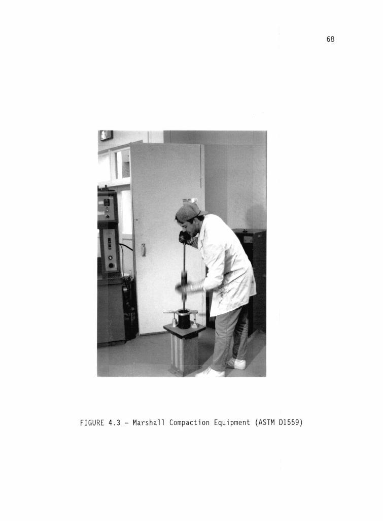
68
FIGURE 4.3 Marshall Compaction Equipment (ASTM D1559)

69
By trial, the required effort for aggregate A was 18 blows/face
and for aggregate B was 23 blows/face to yield approximately 8% air
voids. A summary of the air voids achieved are:
ave. s.dev. cv
Aggregate A (no cure) 9.37 0.34 3.6%
Aggregate A (24 hr cure) 9.10 0.32 3.5%
Aggregate B (no cure) 8.32 0.37 4.5%
Aggregate B (24 hr cure) 8.17 0.41 5.0%
(statistics based on 4 specimen/group)
4.3.3 Kneading Compaction (ASTM D1561)
The standard test procedure followed for preparation of AC mix
specimens by the Kneading Compactor was in general accordance with
ASTM D1561 (1987f), "Preparation of Bituminous Mixture Test Specimen
by Means of the California Kneading Compactor".
In this procedure, a 3.1 in.2 compactor foot is applied to the
mix surface in a 4inch diameter mold by a hydraulic ram. A Cox CS-
1000 California Kneading Compactor was used for compaction (see Figure
4.4). The standard ASTM procedure recommends compaction of the
asphaltaggregate mix at 230°F. A precompaction effort of 20 tamping
blows at 250 psi is required prior to the full compaction of 150
tamping blows at 500 psi. The precompaction effort is recommended to
"form the mixture into a semicompacted condition so that it will not
be unduly disturbed by the full pressure..."(ASTM, 1987f). Following
the precompaction, the compaction mold is allowed to move sidetoside
1/8 inch during the full compaction effort. This allows the kneading
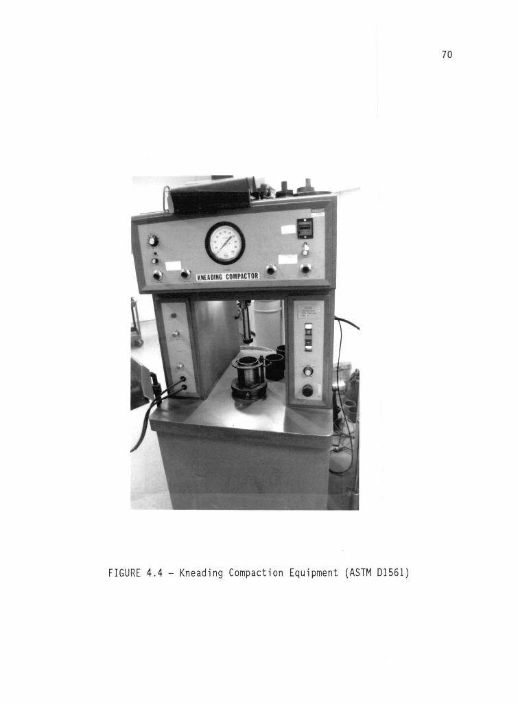
70
FIGURE 4.4 Kneading Compaction Equipment (ASTM D1561)

71
action. The base and sample mold unit are rotated 50° between tamping
blows to assure equal coverages per sample surface. At the conclusion
of the full compaction, the specimen and mold together are placed in a
constant temperature oven at 140°F for 90 minutes. Following the
constant temperature conditioning, the faces of the molded specimen
are "leveled" by means of a double plunge static load of 12,000 pounds
applied at a rate of 0.25 inch per minute. The specimen is allowed to
cool prior to extruding from its compaction mold.
In order to achieve the desired 8% air voids, deviations from
these standards were necessary. By trial, the required effort for
aggregate A was 20 tamping blows precompaction and 50 tamping blows
full compaction, and for aggregate B was 20 and 100. A summary of the
air voids achieved are:
ave. s.dev. cv
Aggregate A (no cure) 7.09 0.27 3.8%
Aggregate A (24 hr cure) 7.07 0.13 1.8%
Aggregate B (no cure) 8.40 0.28 3.3%
Aggregate B (24 hr cure) 8.19 0.29 3.5%
(statistics based on 4 specimen/group)
4.3.4 Gyratoryshear Compaction (ASTM D4013)
The Gyratoryshear specimen were compacted in general accordance
with the specifications presented as ASTM D4013 (1987g), "Preparation
of Test Specimens of Bituminous Mixtures by Means of Gyratory Shear
Compactor" (see Figure 4.5).

72
FIGURE 4.5 Gyratoryshear Compaction Equipment (ASTM D4013)

73
The loose mix is first cured in an oven at 140+10°F to a constant
weight, then transferred to a heated mold and base plate beneath the
ram of the press. The ram is pumped down into the center of the fl
inch diameter mold until the 3.985inch diameter face of the ram makes
contact with the surface of the mixture. Pumping is continued until
the low pressure gage reaches the pregyration stress point of 31.8 psi
(400 lbf.). The mold is immediately tilted to a specified angle of
gyration (up to 12°). The mold is then gyrated 3 times, stopped, and
squared back to a 0° tilt. One full stroke of the metering pump is ap
plied. By observation of the low pressure gage, when an end point
stress of 95.3 psi (1,200 lbf.) is obtained after one full stroke, the
gyratoryshear compaction is completed. If the end point stress is
not achieved, the method is repeated.
After completion of the gyratoryshear compaction, at
approximately one stroke per second, the pressure is pumped up to 1590
psi (20,000 lbf.) for consolidating the mix. The specimen is allowed
to cool in the mold, then extruded.
In order to compact the specimen to 8% air voids, a 1° angle of
gyration was used at a compaction temperature of 275°F. An end point
stress of 100 psi was also used. A summary of the air voids achieved
are:
ave. s.dev. cv
Aggregate A (no cure) 8.07 0.26 3.2%
Aggregate A (24 hr cure) 7.83 0.22 2.8%
Aggregate B (no cure) 7.95 0.25 3.1%
Aggregate B (24 hr cure) 7.97 0.26 3.3%
(statistics based on 4 specimen/group)

74
4.4 Analysis and Results
Mr tests were performed on each sample using the RepeatedLoad
Test System. Both the 40°F and 73°F test temperatures were evaluated,
and the standard test conditions of 0.1 second load duration, 0.33
hertz load frequency and a microstrain level between 50 and 60 were
also used.
The assumption of consistent replicated specimens is nearly met
in that the cv of air voids for any combination of compaction and
curing shown in the previous pages does not exceed 5% .
Results of the testing are given in Table 4.2. This table shows
the computed means of each treatment combination with the associated
standard deviations (s.dev.) and coefficients of variation (cv) based
on 4 specimens per group.
The analysis of the 40°F test results are presented in Table 4.3.
Similarly, Table 4.4 presents analysis of the 73°F test results. Both
resulted in a highly significant (at the 0.01 alevel) Fratio of the
second order (AxBxC) interaction, suggesting that none of the three
factors act independently on the resilient modulus, and that
differences between interactive treatment means exist.
Once again, the lower temperature leads to greater precision than
the higher temperature. This is supported by the comparison of the CV
between the two experiments. This finding further supports the
conclusion made in the Parametric Study that lower testing
temperatures lead to more precise Mr values. Thus the 73°F results
were dropped from the remaining analysis.
A summary of the results at 40°F are shown in Table 4.5. The
treatment groups means and standard error of means are given, as well
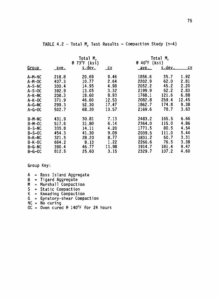
75
TABLE 4.2 Total Mr Test Results Compaction Study (n=4)
Total M Total Mr
@ 73°F (ksi) @ 40°F (ksi)
Group ave. s.dev. cv ave. s.dev. cv
A-M-NC 218.8 20.69 9.46 1856.6 35.7 1.92
A-M-OC 407.3 10.77 2.64 2202.9 62.0 2.81
A-S-NC 300.4 14.95 4.98 2052.2 45.2 2.20
A-S-OC 392.9 13.05 3.32 2199.9 62.2 2.83
A-K-NC 208.3 18.60 8.93 1768.1 121.6 6.88
A-K-OC 371.9 46.60 12.53 2082.8 259.4 12.45
A-G-NC 299.3 52.30 17.47 1862.7 174.8 9.38
A -G -OC 502.7 68.20 13.57 2169.6 78.7 3.63
B-M-NC 431.9 30.81 7.13 2483.2 165.5 6.66
B-M-OC 517.6 31.80 6.14 2364.0 115.0 4.86
B-S-NC 335.8 14.11 4.20 1771.5 80.5 4.54
B-S-OC 454.3 41.30 9.09 2039.5 111.0 5.44
B-K-NC 321.5 28.20 8.77 1831.2 60.7 3.31
B-K-OC 664.2 8.13 1.22 2266.6 76.5 3.38B-G-NC 390.4 46.77 11.98 1914.7 181.4 9.47
B -G -OC 812.5 25.60 3.15 2329.7 107.2 4.60
Group Key:
A = Ross Island AggregateB = Tigard AggregateM = Marshall CompactionS = Static CompactionK = Kneading CompactionG = Gyratory-shear CompactionNC = No curingOC = Oven cured @ 140°F for 24 hours

76
TABLE 4.3 ANOVA for Total Mr at 40°F
Source ofVariation
Degrees ofFreedom
Sum ofSquares
MeanSquare Fratio
Total 63 3,715,108
A 1 162,812 162,812 11.4**
B 1 1,118,306 1,118,306 78.5**
AxB 1 3,423 3,423 0.2
C 3 547,129 182,376 12.8**
AxC 3 756,605 252,202 17.7**
BxC 3 190,063 63,354 4.4**
AxBxC 3 253,266 84,422 5.9**
Error 48 683,504 14,240
** Significant at the a = 0.01 level CV = 5.8%

77
TABLE 4.4 ANOVA for Total Mr at 73°F
Source ofVariation
Degrees ofFreedom
Sum ofSquares
MeanSquare Fratio
Total 63 1,518,169
A 1 376,076 376,076 342.34*
B 1 653,672 653,672 595.0t*
AxB 1 25,760 25,760 2144*
C 3 167,044 55,681 50.7**
AxC 3 63,168 21,056 19.2**
BxC 3 114,348 38,116 34.74*
AxBxC 3 65,371 21,790 19.84*
Error 48 52,730 1,099
** Significant at the a = 0.01 level CV = 8.0%

78
TABLE 4.5 Summary of Modulus Means, Standard Errors, andSignificant Differences at 40°F
Total Resilient Modulus@ 40°F (ksi)
(statistics of four replicates)
Group Mean (ksi) Standard Error of Mean (ksi)
A-M-NC -1856.6 (MSE/r)4 = (14,987/4)4 = 61.2
A-M-OC - 2202.9A-S-NC 2052.2-1
A-S-OC - 2199.9-JA-K-NC -1768.1A-K-OC 2082.8
A-G-NC - 1862.7
A -G -OC ---2169.6
B-M-NC 2483.2-1
B-M-OC ---2364.0-J
B-S-NC 1771.5
B-S-OCB-K-NC
[2039.51831.2
B-K-OC - 2266.6B-G-NC 1914.7
B-G-OC 2329.7AA
Equal Equal
CompactionMethods*
CuringMethods*
*Standard Error for Differences:SE = (2MSE/r)4 = 86.6 ksi
Group Key:
A = Ross Island AggregateB = Tigard AggregateM = Marshall CompactionS = Static CompactionK = Kneading CompactionG = Gyratory-shear Compaction
NC = No curingOC = Oven cured @ 140°F for 24 hours

79
as links of equal means as governed by the tstatistic of interactive
treatment mean differences [standard error for differences =
(2MSE/0112, where r = no. of replicated specimens = 4] at the 0.05 a
level.
In general, all methods of compaction yield similar Mr results,
as shown on the left side of the means column in Table 4.5. However,
the following exceptions to this generalization exist. The Static
method yielded Mr values distinctly different from the other 3 methods
for Aggregate A with no oven curing. Similarly, the Marshall method
yielded different Mr values for Aggregate B with no oven curing, and
the Static method yielded different Mr values for Aggregate B with the
oven curing treatment. The comparisons were made using a ttest
between means.
Also of interest are the differences in Mr values between curing
procedures at each level of aggregate type and compaction method.
From Table 4.5, as shown on the right side of the means column, the
Static method did not yield significantly different Mr values between
curing procedures for Aggregate A, and the Marshall method for
Aggregate B.
From the previous discussion, choosing either the Kneading or the
Gyratoryshear methods of compaction appears warranted. The selection
between the two can be made by observing the cv column shown in Table
4.2. This method of selection suggests choosing the compaction method
that results in the lowest cv (implying the best accuracy in Mr
results). By observation, it would appear that the Kneading
compaction method without the oven cure precompaction conditioning may

80
be the best. However, it could be reasonably argued that any method
of compaction could meet this requirement.
Further, the Kneading method or the Gyratoryshear method of
compaction are leading candidates for laboratory compaction based on
the acceptible ability to simulate field compaction with respect to
material properties (Consuegra et al., 1989).
4.5 Conclusions and Recommendations
Based on the evaluation of these study results, the following
conclusions appear warranted:
1. For any of the 4 methods of compaction, the 2 methods that
result in the highest differences between modulus values of
2 methods of preconditioning are the Kneading compaction
and the Gyratoryshear compaction.
2. The desired method of compaction and conditioning based on
repeatable modulus values is the Kneading compaction
without the oven cure preconditioning.
From the conclusions made, the recommended compaction method to
be used for the improved test method to determine the degree of
asphalt stripping from aggregates is the Kneading compaction (ASTM,
1987f).

81
5 PRIMARY FACTORIAL STUDY
This chapter presents results of a concentrated laboratory study
to evaluate the effects of asphalts, air voids and antistripping
additives on stripping. The following sections provide a format for
the analysis of results with specific questions of interest to be
answered. The preparation of the test specimen is described, followed
by a presentation of test results and discussion of the results.
Finally, conclusions and recommendations are summarized for the work
effort.
5.1 Obiectives
Six replicate specimens were prepared for each factorial
combination of treatments identified in the following section. This
number was selected to increase the likelihood of obtaining
significant discrimination between treatment groups without doing an
excessive quantity of testing. The selection is supported by work
done by Kim et al. (1989).
The overall goal of this phase of the study is to evaluate the
sensitivity of the test method to detect moisture damage in AC
specimens. Of primary concern is the ability of the procedure to
strongly differentiate between a stripping aggregate and a non
stripping aggregate. Of equal importance is the ability to show
significant improvement of the mixes containing antistripping
additives over mixes that do not.

82
Prior to testing, a number of specific questions that could be
obtained from this study were generated to aid in the overall
evaluation of the study results:
I. Is there a significant difference in retained moduli (IRMr)
between the partially saturated group and the fully
saturated group?
2. What number of conditioning cycles are required to obtain a
significant drop in the IRMr as compared to that obtained
after a single cycle? Further, does the IRMr cease to
change significantly after some number of cycles?
3. Do the test results indicate differences in the performance
of the 2 aggregate types?
4. Are there significant differences in the IRMr between the
three air void contents within each combination of
aggregate, asphalt and additive?
5. For the stripping aggregate (Agg. B), is the IRMr for the
additive mixtures significantly different than that for the
untreated mixtures at the same air voids level?
6. One would expect that the IRMr would be dependent on
aggregate type, asphalt, additive treatment, air voids and
the number of condition cycles. Therefore, can the
following prediction model (or some transposition) for the
IRMr be fit:
IRMr = flo + X Di(Air) + fl2(Agg.) + 03(Add.) + #4(Asph)] ....(5.1)

83
where #0 = IRMr intercept @ X = 0 (400% for original IRMr)
X = No. of condition cycles
Air = Air voids content (4, 8, 12%)
Agg. = Aggregate type (A=0 or B=1)
Add. = Antistripping additive (none=0, L=1, or P=2)
Asph. = Asphalt type (AR-4000W=0 or AC-20R=1)
/31, /32, #3, /34 = Slope parameters.
The laboratory work effort is outlined in Figure 5.1. A
discussion of the Lottman conditioning used in this study was given in
section 2.2.2.
5.2 Experimental Design
Mixes composed of several material variables are evaluated in
this study, including 2 aggregate types, 2 asphalts, 2 antistripping
additives and 3 air void contents.
Questions 1 and 2 stated above can be answered using a pooled t
test between group means (Devore and Peck, 1986b). The groups as
stated here represent the average IRMr of each cycle of moisture
conditioning over the 18 combinations of material groups [representing
the partial factorial combinations of treatments (2 aggregates x 2
asphalts x 3 air voids) + (1 aggregate x 2 additives x 3 air voids) =
12+6 = 18 treatments]. Each cell within the layout will represent the
average IRMr of the 6 replicates. From this analysis, it is
anticipated that by answering question number 2, an analysis of
variance could be performed on the results at a specific point in time

Recombine aggregatesin exact fractions
I
Prepare trial batches todetermine compoctive effort
to yield 4, 8 and 12%air voids and 2.5in. height
Perform maximum specificgravities on trial samples
(ASTM D 2041)
1
I
Ross Island w/ Ross Island w/ Tigard w/AR4000W AC 20R AR4000W
4% air voids 4% air voids 4% air voids8% air voids 8% air voids 8% air voids12% air voids 12% air voids 12% air voids
6 specimen each 6 specimen each 6 specimen eoch
I
Tigard w/AC 20R
4% air voids8% air voids12% air voids
6 specimen each
I
Tigard w/AR4000W& 1% lime
4% air voids8% air voids12% air voids
6 specimen each
Tigard w/AR4000W & 0.5%Pave Bond Special
4% air voids8% air voids12% air voids
6 s ecimen each
Condition and testspecimen per Figure 5.2
FIGURE 5.1 Laboratory Program Factorial Study

85
(i.e., following some determined number of conditioning cycles). This
analysis can be accomplished using a completely randomized design
(CRD) with the same 18 combinations of material groups selected as
treatments (Peterson, 1985a). By using the computed Ftrtratio from
the ANOVA (as shown in Table 5.1), the null hypothesis of equal
treatment means can be tested against the alternative hypothesis that
treatment means are different. For the test procedure to be sensitive
to material changes, it is desired to observe a significant Ftrtratio,
that is, be greater than the critical Fratio for the associated
degrees of freedom and significance level.
Specific differences between treatment means can then be tested
using the ttest statistic, where the standard error of differences is
given by (2MSE/r)112, and r is the number of replicated specimens
(Peterson, 1985a).
The factorial set of samples were tested for total Mr using the
RepeatedLoad Diametral Test System described in Section 2.1. The
following sections describe the methods used to prepare the test
specimens.
5.2.1 Materials
Aggregates. Two aggregates were used in this study. Aggregate A
is from Ross Island Sand and Gravel. This aggregate is a crushed
riverrun aggregate dredged in the Willamette River in Portland,
Oregon. This aggregate has been observed to resist stripping in local
area projects. Aggregate B is from Tigard Sand and Gravel. This
aggregate is a hillside quarried crushed rock, and has been known to

86
TABLE 5.1 Experimental Design ANOVA Primary Factorial Study
Source of Degrees of Sum of MeanVariation Freedom Sauares Square Fratio
Treatments n-1 = 17 SST MST Ft rt
Error n(r-1)=90 SSE MSE
Total rn-1 = 107 SSTot

87
strip excessively in Portland area projects. Portland has a wet,
moderate climate which experiences occasional winter freeze.
Properties of these aggregates were presented in Section 2.3 of this
report.
Asphalts. Two asphalts were evaluated in this study. The AR-
4000W and AC-20R(R) were discussed in Section 2.3.3.
Antistripping Additives. Hydrated lime(L) and PaveBond
Special(P) were evaluated for the effects in stripping for the B
aggregate. Properties of these additives were given in Section 2.3.3.
It should be noted that this design is not a full factorial
because the full range of combinations were not used, specifically,
the antistripping additives were not used for aggregate A, the known
nonstripper.
Air Voids. It was desirable to prepare the laboratory compacted
samples over a broad range of typical field air void values.
Therefore, 4, 8, and 12% air voids were selected for each factorial
combination discussed above. Air voids were determined by the
standard test procedure given in ASTM D3203 (1987c), "Percent Air
Voids in Compacted Dense and Open Bitumnous Paving Mixtures". Bulk
specific gravities of the compacted specimen were determined in
accordance with ASTM D2726 (1987d), "Bulk Specific Gravity and Density
of Compacted Dense and Open Bituminous Paving Mixtures". The actual
air voids achieved are presented later in this chapter.

88
5.2.2 Specimen Preparation
Six replicate specimens were prepared for each of the 18
factorial combinations; therefore, a total of 108 specimens were
prepared for testing in this study. The following sections discuss
the batching and mixing process, followed by a summary of the
compactive effort required for each mixture at each air void level.
Batching and Mixing. Each aggregate was recombined from 7
separated stockpile sizes to meet the mix design gradation as supplied
by the Oregon Department of Transportation. These densegraded mix
gradations were discussed in Section 2.3.3 of this report. The total
weight of aggregate was adjusted to obtain a specified 2.5inch
specimen height recommended for modulus testing. The recombined
aggregate was placed in a 310°F oven to drive off surface water and
bring the aggregate above the mixing temperature of 305°F.
Asphalt was added to the aggregate at a rate supplied by ODOT and
presented in Chapter 2. ODOT mix designs are based on the Hveem
Method of Mix Design and the asphalt content is presented as a
percentage of the total weight of mix. The asphalt content of
aggregate A is 5.9% and for B is 6.6%.
A discussion of the antistripping additives and how they were
added to the aggregate B mixtures were presented in Section 2.3.3.
Mixing was done by means of a Cox mechanical mixer. Mixing time
was two minutes at 305°F.

89
Kneading Compaction. Compaction of the mixtures was done in
general accordance with ASTM D1561 (1987f), "Preparation of Bituminous
Mixture Test Specimen by means of the California Kneading Compactor",
which was selected for this study on the basis of conclusions and
recommendations made in the previous chapter.
Deviations from the standard method presented in ASTM D1561 were
necessary to achieve the level of air void contents desired. The
standard recommends a compaction temperature of 230°F, a precompaction
effort of 20 tamping blows at 250 psi and a full compaction effort of
150 tamping blows at 500 psi. Table 5.2 is a summary of the average
air voids of 6 replicates per group achieved along with the associated
standard deviations. Also included is a summary of the deviations to
the recommended compaction effort required to achieve those air void
contents.
By observation of Table 5.2, the level of air voids achieved do
not necessarily match the target air voids desired. However, the
range of air voids (5.12 to 10.99%) should be great enough to show the
effects of air voids with respect to moisture sensitivity.
5.3 Test Results
Moisture conditioning of specimens continued until the cycling
led to a 50% loss in original Mr (i.e., IRMr< 50%) of the control
specimen (i.e., aggregates w/AR-4000W and no antistripping
aggregates). By observation of test results, this criteria occurred

90
TABLE 5.2 Summary of Kneading Compaction Effortand Air Voids Achieved Factorial Study
SampleGroup
Number of tamping blowsAir Voids, %Pre- Full
Compaction Compaction Compaction@ 250 psi @ 500 psi Temp.°F.
(6 replications/group)ave. s.dev. cv
A4 20 150 250 5.12 0.20 3.9
A8 20 85 230 8.12 0.45 5.5
Al2 30 0 220 10.00 0.32 3.2
AR4 20 150 250 5.46 0.84 15.4
AR8 20 35 230 7.14 0.41 5.7
AR12 30 0 220 8.87 0.37 4.2
B4 20 150 260 6.44 0.59 9.2
B8 20 95 230 7.65 0.61 8.0
B12 25 0 215 10.07 0.77 7.7
BR4 20 150 260 6.09 0.37 6.1
BR8 20 95 230 6.91 0.45 6.5
BR12 25 0 215 9.50 0.33 3.5
BP4 20 150 260 5.63 0.34 6.0
BP8 20 95 230 6.78 0.48 7.1
BP12 25 0 215 10.99 0.56 5.1
BL4 20 150 260 5.49 0.31 5.7
BL8 20 95 230 6.17 0.54 8.8
BL12 25 0 215 9.21 0.31 3.4
Sample Group Key:
A = Aggregate AB = Aggregate BR = AC-20R (all others without R are mixed with AR-4000W)
P = PaveBond SpecialL = Lime4, 8 and 12 = target air voids,%

91
following the 5th freezethaw cycle. Therefore, the number of con
ditioning cycles used for all specimen groups was 7, shown below:
Cycle #1 = partial saturation
Cycle #2 = full saturation
Cycle #3 = freezethaw cycle #1
Cycle #4 = freezethaw cycle #2
Cycle #5 = freezethaw cycle #3
Cycle #6 = freezethaw cycle #4
Cycle #7 = freezethaw cycle #5
The IRMr results for aggregate A (the nonstripper) is shown in
Figure 5.2. Likewise, the results for aggregate B (the stripper) is
shown in Figure 5.3. These graphs show the IRMr plotted against the
successive stages of moisture conditioning, and each bar represents an
average of the 6 replicated specimen results. These graphs are
intended to visually show the significance of the IRMr resulting from
the analysis described below.
The results of the testing are summarized in Table 5.3, with 7
columns of condition cycles and 18 rows of material groups (i.e., a
combination of materials and air voids). A number of relationships
can be derived from this table, with the comparison of successive
column means by use of the pooled ttest shown at the bottom. These
include:
1. The difference between partially saturated specimen and
fully saturated specimen is insignificant (the probability

!Mir.
TRW.
100
95
90
B5
BO r-
75F-
70
dry PAW. flit. IF-T 2F-T 3F-T
Condition Cycles
4F -7 5F -7
a) Aggregate Type A 4% air voids
60 r-
L:SO
45
40
TRW. S
100
95
90
95
90
75
10
65
60
55
50
45
40
dry f.set. IF-1 2F-T
Condition Cycles
3F -7 4F -7 5F -T
b) Aggregate Type A 8% air voids
dry orset. f.sat. IF-T 2F-T 3F-T
Condition Cycles
4F -7 5F -T
1111111 IRN no oddItIve
EZZ2 IRN wIAC-2011
1111111 TRU no adOitive
2223 IAN w/AC-20R
1111111 IN no slooltive
Ez2s2 IRA w/AC-20R
c) Aggregate Type A 12% air voids
FIGURE 5.2 IRMr vs. Condition Cycles Aggregate A
92

IRM-, %
IOC N95 h-
90 L.
es
80 --
75
70
65 L_
60
55
50 :45
40 L_ LU
%
100
95 L_
90 --
85 --
BC --
75
7C --
E5
60 --
55 ',-
SO
45 H-
41aei
p.sat. f.gat. 15-T 25-7 35-T
Condition
45-T 55-T
a) Aggregate Type B 4% air voids
100
95
90
85
BC
75
70
65
60
55
5C
45
40
V
S
P.Sat. f.sat. 15-1 2F-T 35-T 45-T
Condition Cyples
5=-7
b) Aggregate Type B E% a:7" 'voids
35-T 4=-7 5F-T
F-7772 IRM no additive
IIIIII 'RR w/PaveBond Spec.
7/721 IRM et% Lime
ZZZ IRm 47,20R
t"NN IRM no additive
MINIIRM w/BaveBond Spcp.
IRM wit% Liu
IRM 402OR
TAM is alCitivs
TAM o/Pave9cnci Spcc.
IRM w11% ._imc
IRM ACCC,A
c) Aggregate Type B 12% air voids
FIGURE 5.3 IRM, vs. Condition Cycles Aggregate B
93

94
TABLE 5.3 - Summary of IRMr (%) Test Results and Analysis (n=6)
Index of Retained Modulus,
MATERIALS
CONDITION CYCLES
1
Partially
Saturated
2
Fully
Saturated
3
Freeze
Thaw #1
4
Freeze
Thaw #2
5
Freeze
Thaw #3
6
Freeze
Thaw #4
7
Freeze
Thaw #5
A4 102.35 101.78 80.60 68.47 59.07 54.89 49.21
A8 94.99 90.45 74.77 67.81 63.49 54.81 50.70
Al2 89.70 92.64 87.96 74.78 69.37 58.7,4 51.04
AR4 95.76 91.29 88.23 86.14 80.20 77.07 76.63
AR8 93.76 89.06 81.48 69.89 67.09 70.09 68.07
AR12 91.10 89.46 91.50 91.90 83.02 78.59 68.83
BR4 91.91 92.79 74.90 65.38 63.63 60.01 59.01
BR8 92.23 90.47 78.17 76.54 70.44 66.28 66.53
BR12 90.26 92.34 81.95 80.09 74.90 71.13 65.03
B4 103.62 98.81 68.20 61.48 55.64 51.79 51.02
B8 94.95 92.84 66.67 61.27 58.13 50.81 49.91
B12 87.15 89.85 71.00 67.50 62.17 56.20 48.81
BP4 90.62 88.79 64.21 59.52 54.54 51.71 49.22
BP8 96.65 90.25 70.33 65.85 60.26 58.49 57.17
BP12 98.80 97.39 83.86 82.97 77.52 73.66 68.20
BL4 95.53 88.71 66.04 60.16 51.70 48.26 45.35
BL8 90.95 90.57 69.98 60.81 54.49 53.09 51.98
BL12 92.54 95.29 74.76 66.28 55.88 50.15 48.30
block mean 94.05 92.38 76.37 70.38 64.53 60.32 56.95
variance 18.70 13.67 68.66 92.88 90.83 97.73 89.34
size 18 18 18 18 18 18 18
t statistic 1.247 7.486 1.999 1.831 1.301 1.047
degrees of freedom 33 24 33 34 34 34
t crit: 0.05 level 2.04 2.07 2.04 2.04 2.04 2.04
0.01 level 2.75 2.81 2.75 2.75 2.75 2.75
* *
links of equal means
0.05 level
O 0.01 level
** highly significant difference at the 0.01 level

95
that they are equal is greater than 2 in 10). This
accepted hypothesis that the mean IRMr of the two groups
are equal is shown as an insignificant tstatistic in the
comparison of column means. This opposes the findings of
Tunnicliff and Root (1984).
2. There is a highly significant difference in IRMr between
saturated specimen and specimen subjected to one freeze
thaw cycle (the probability that they are equal is less
than 1 in 1000), shown as a highly significant tstatistic
in the comparison of successive column means.
3. There are insignificant differences in IRMr following the
first freezethaw cycle (the probability that they are
equal is greater than 5 in 100), shown as insignificant t
statistics in the comparison of successive column means.
Two tables similar to Table 5.3 were prepared prepared for the
results of each aggregate. Table 5.4 presents results and analysis
for only aggregate B. Similarly, Table 5.5 represents aggregate A.
By comparison of column means for these tables, the above
relationships hold true, with exception to number 2. For aggregate B
(the stripper), there remains a highly significant drop in IRMr between
saturated specimen and specimen subjected to one freezethaw cycle
(the probability that they are equal is less than 1 in 1000).
However, for aggregate A (the nonstripper), that same difference is
not highly significant (the probability that they are equal is greater
than 1 in 100 and less than 5 in 100). This is a significant finding.

TABLE 5.4 -Summary of IRMr (%) Test Results and Analysis for
Aggregate B (n=6)
Index of Retained Resilient Modulus. X (n.6)
MATERIALS
CONDITION CYCLES
1
Partially
Saturated
2
Fully
Saturated
3
Freeze
Thaw #1
4
Freeze
Thaw #2
5
Freeze
Thaw #3
6
Freeze
Thaw #4
7
Freeze
Thaw #5
BR4 91.91 92.79 74.90 65.38 63.63 60.01 59.01
BR8 92.23 90.47 78.17 76.54 70.44 66.28 66.53
BR12 90.26 92.34 81.95 80.09 74.90 71.13 65.03
84 103.62 98.81 68.20 61.48 55.64 51.79 51.02
B8 94.95 92.84 66.67 61.27 58.13 50.81 49.91
B12 87.15 89.85 71.00 67.50 62.17 56.20 48.81
BP4 90.62 88.79 64.21 59.52 54.54 51.71 49.22
BP8 96.65 90.25 70.33 65.85 60.26 58.49 57.17
BP12 98.80 97.39 83.86 82.97 77.52 73.66 68.20
BL4 95.53 88.71 66.04 60.16 51.70 48.26 45.35
BL8 90.95 90.57 69.98 60.81 54.49 53.09 51.98
BL12 92.54 95.29 74.76 66.28 55.88 50.15 48.30
block mean 93.77 92.34 72.51 67.32 61.61 57.63 55.04
variance 19.68 10.86 39.78 65.93 72.13 72.96 62.65
size 12 12 12 12 12 12 12
t statistic 0.894 9.655 1.747 1.684 1.144 0.770
deaees of freedom 20 17 21 22 22 22
t critical: 0.05 level 2.09 2.11 2.08 2.07 2.07 2.07
0.01 level 2.85 2.90 2.83 2.82 2.82 2.82
**
links of equal means
96
@ 0.05 level
0 0.01 level
** highly significant difference at the 0.01 level

97
TABLE 5.5 Summary of IRMr ( %) Test Results and Analysis forAggregate A (n=6)
Index of Retained Resilient Modulus. .
MATERIALS
CONDITIONING CYCLES
1
Partially
Saturated
2
Fully
Saturated
3
Freeze
Thaw #1
4
Freeze
Thaw /2
5
Freeze
Thaw 03
6
Freeze
Thaw 04
7
Freeze
Thaw 05
A4 102.35 101.78 80.60 68.47 59.07 54.89 49.21
A8 94.99 90.45 74.77 67.81 63.49 54.81 50.70Al2 89.70 92.64 87.96 74.78 69.37 58.74 51.04
AR4 95.76 91.29 88.23 86.14 80.20 77.07 76.63
AR8 93.76 89.06 81.48 69.89 67.09 70.09 68.07
AR12 91.10 89.46 91.50 91.90 83.02 78.59 68.83
block mean 94.61 92.45 84.09 76.50 70.37 65.70 60.75
variance 19.71 22.57 38.58 103.35 88.69 119.72 139.90
size 6 6 6 6 6 6 6
t statistic 0.815 2.618 1.561 1.083 0.793 0.753
degrees of freedom 10 9 8 10 10 10
t critical: 0.05 level 2.23 2.26 2.31 2.23 2.23 2.23
0.01 level 3.17 3.25 3.36 3.17 3.17 3.17
@ 0.05 level
links of equal means
@ 0.01 level
" significant differences at the 0.05 level
* highly significant differences at the 0.01 level

98
The suggestion is to observe IRMr values obtained after one freezethaw
cycle to analyze the differences in treatments.
This suggested comparison was accomplished using a CRD with the
same 18 treatments (see Table 5.1). Table 5.6 shows these results,
and the highly significant Ftrt indicates that differences between
treatment means exist.
Table 5.7 represents results of specific treatment group
comparisons following one freezethaw cycle. The following
comparisons are true:
1. There exists a highly significant difference in IRMr
between the two aggregates (the probability that they are
equal is less than 1 in 100). Aggregate A has a higher
IRMr than Aggregate B, suggesting that A does not strip to
the same extent as B.
2. The effectiveness of additives on aggregate B (the known
stripper) is highly significant at 12% air voids for the
PaveBond additive. No other comparison between additive
vs. control are significant.
3. The effectiveness of the AC-20R to reduce stripping of
aggregate B is highly significant at 8 and 12% air voids
(the probability that they are equal to the comparitive
control group is less than 1 in 100) and significant at 4%
air voids (the probability that that they are equal to the
comparitive control group is greater than 1 in 100 and less
than 5 in 100).

99
TABLE 5.6 Summary of IRMr Results Following One Freeze-thaw Cycle
Source ofVariation
Degrees ofFreedom
Sum ofSquares
MeanSquare F-ratio
Treatments 17 7010 412 16.1**
Error 90 2300 26
Total 107 9310
** Significant at the 0.01 level

TABLE 5.7 Significant Differences of Treatment MeansFollowing One Freezethaw Conditioning Cycle
GroupComparison Significance
Effect ofAdditivesat similaraggregatetype andair voidscontent
Effect ofAir Voidsat similaraggregatetypes andadditivetypes
A4AR4A8AR8Al2AR12B4BR4B8BR8B12BR12B4BP4B8BP8B12BP12B4BL4B8BL8B12BL12
* **
* *
100
A4A8 + *A4Al2 **A8Al2 **AR4AR8 + *AR4AR12AR8AR12 **B4B8 +B4B12B8 B12BR4BR8BR4BR12BR8BR12BP4BP8 *BP4PB12 **BP8BP12 **BL4BL8BL4BL12 **BL8BL12
Minus () sign shows higher air voidswith higher IRMr
Effect of A4B4aggregate A8B8type at Al2B12similar air AR4BR4voids and AR8BR8asphalt type AR12BR12 **
********
KEY: *Significant difference**Highly significant difference

101
4. With exception to group comparisons A4A8, AR4AR8 and B4
B8, all comparisons show that the higher air voids content
have higher IRMr. Table 5.7 shows which differences are
significant.
A prediction model similar to the one given in equation 5.1 can
be fit with the data presented in Figures 5.2 and 5.3. Because the
test results indicate a significant drop in the IRMr from full
saturation to the first freezethaw cycle, and insignificant drops in
successsive freezethaw cycles, a model could be developed to predict
the IRMr of successive freezethaw cycles based on the IRMr after the
first freezethaw cycle. Therefore, a fit to the following model was
sought:
IRMr = /30 + X[fliagg + $2air + p3add + $4asph] (5.1)
where: flo = IRMr intercept at X = 0X = No. of freezethaw cycles
1 = freezethaw#12 = freezethaw#23 = freezethaw#34 = freezethaw#45 = freezethaw#5
all other variables defined as before
The computer program STATGRAPHICS (1987) was used to help in the
analysis of the least squares fit. By trial, error, and observation
of residuals (nonuniform) resulting from the model given as equation
5.1, it was determined that a logrithmic (most likely an exponential
decay) model would provide a better fit of the data. Therefore, the

102
IRMr results obtained in the laboratory were transformed by the natural
logarithm, and the following model was fit:
ln(IRMr) = flo + X[fllagg + /32air + fl3add + #4asph] (5.2a)
or, rewritten
IRMr = exp(00)exp[X(fliagg + fl2air + 03add + $4asph)] (5.2b)
The least squares fit of this model resulted in the conclusion
that "add" (additive type) variable did not add a great deal to the
fit of the model (the probability that the "add" slope parameter fl3 is
zero is greater than 2 in 10). Therefore the additive type predictor
variable was dropped from the model, and the following model was fit:
IRMr = exp(4.3115)exp[x/100(-3.7agg 0.49air + 4.3asph)] ...(5.3)
The coefficient of determination (R2) resulting from this model fit was
0.48, indicating about 48% of the observed variability in the IRMr is
modeled by the predictor variables (air voids, aggregate type, and
asphalt type). There is no basis to determine if R2 is small or large
without a lot of experience in problems like this.
5.4 Discussion of Results
As one would have hoped, the Mr test employed for this study was
sensitive to material changes. Of primary concern was the ability to
discriminate between IRMr of two types of aggregates, namely a proven
stripper and a proven nonstripper. The comparison can be made
following the first freezethaw cycle.

103
Because the test is nondestructive, a minimum number of
replicates need to be prepared for any group that a user wishes to
compare. Kim et al. (1989) suggests using 6-8 replicate specimens for
moisture susceptibilty tests. The comparison has the potential to be
much more precise than destructive test procedures because the same
sample that is tested dry and recorded as the base Mr in the IRMr ratio
is also tested following successive moisture condition cycles, thus
reducing the error associated with testing replicate sample groups.
The advantage of the IRMr test over destructive retained strength tests
(i.e., splittension) is increased precision with fewer samples re
quired to perform the tests.
One result of this experiment was the effectiveness (or non
effectiveness) of additives. In all but two cases (B4BP4 and B4
BL4), the effect of additive treatment was positive (i.e., resulted in
a higher IRMr than the control group). However, the testing was not
sensitive enough to detect these effects as being significant, with
the exception of the PaveBond Special treatment at high air voids.
The AC-20R polymer modified asphalt appears to be effective for
reducing stripping potential in the densegraded mixes. Through
separate studies, rubber asphalts may perform better at lower extreme
temperatures than conventional grade asphalts, and their resistance to
fatigue appears higher than comparable conventional grade asphalt
mixes (Scholz et al., 1987).
Another result of this study was the effect that air void
contents have on the IRMr. In most cases, the IRMr was higher for high
air voids. One explanation for this could be the procedure used in
the freezethaw cycles (Lottman, 1978). The recommended procedure for

104
freezing a specimen following a full saturation treatment is to
tightly wrap the specimen in a double layer of thin plastic. This is
suggested to hold the pore water in the specimen air voids and to
prevent drying during the freezing process. The wrapped specimen is
then placed in a sealed plastic bag with 10 milliliters of distilled
water. This second application is intended to further reduce drying
of the specimen. The bagged specimen is transferred to a freezer (0°F
± 3.6°F) for 15 hours. After freezing, the specimen is unwrapped and
placed in a distilled hot water bath.
If done properly, the fully saturated specimen (full saturation
implies all voids in the specimen are completely filled with water)
will freeze with all voids completely full of water. This in turn
will lead to substantial void volume changes due to the expansion of
pore water to ice. However, by observation, the higher air void
groups partially drained from top to bottom prior to freezing, and the
lower air void groups did not drain as much, implying that the lower
air void groups would probably show a relatively larger change in air
voids due to the freezing condition. This could explain why the lower
air void groups generally showed lower retained modulus ratios (IRMr)
than the higher air void groups.
After testing was completed and the effect of air voids on the
IRMr was detected, the air void content for each sample were
redetermined using the following technique. All samples were air
dried at room temperature for 5 months following the 5th freezethaw
cycle. One group of 6 specimen (AR4) was then subjected to a 48hour
vacuum dessication and another group (B4) to a 48hour 120°F oven. It
was determined that neither method of drying proved to drive off any

105
remaining water, therefore all samples were assumed "dry" after the 5
month storage at room temperature. In all cases, a range of 4 11
grams of water were retained by the samples after the 5th freezethaw
cycle and following the "drying" period (implies less than 1% moisture
retention for a 1200 gram specimen). Therefore, the new air voids
were determined using the original dry weight of each specimen, and
the respective buoyant and saturated surface dry weights of the
conditioned specimen for the calculation of air voids presented in
ASTM D-2726 (1987d).
Table 5.8 shows the comparison between the average air voids per
group at the dry state and the redetermination of the same specimen
following the 5th freezethaw cycle. The change in air voids shown in
this table illustrates a trend of greater changes for the lower air
void groups and smaller changes for the higher air void groups. This
trend suggests that the conditioning process may negatively bias low
air void groups. The process was developed for samples compacted to
7-8 percent air voids (Lottman, 1978).
The change in air voids also suggests damage to the specimen that
is not stripping. It has been shown in previous studies that the Mr is
sensitive to air void contents (Hicks et al., 1985). Therefore, the
final Mr values obtained after the 5th freezethaw cycle were corrected
for the change in air voids. By correcting for air void changes, one
can visualize damage to the specimen that can only be attributed to
moisture damage. The correction to the Mr was determined using a
sensitivity analysis presented in Transportation Research Record, 1034
(Akhter and Witczak, 1985). The results of this sensitivity analysis
are presented in Table 5.9. The final column in this table represents

106
TABLE 5.8 Air Void Content ComparisonBefore and After Conditioning
SampleGroup
Pre-testing Air Voids,%Ave. S.Dev.
Post Testing Air Voids,%Ave. S. Dev. Change
A4 5.12 0.20 6.53 0.19 1.41A8 8.12 0.45 9.31 0.28 1.19Al2 10.00 0.32 10.89 0.34 0.89AR4 5.46 0.84 6.36 0.64 0.90AR8 7.14 0.41 8.44 0.41 1.30AR12 8.87 0.37 10.47 0.58 1.60B4 6.44 0.59 7.89 0.57 1.45B8 7.65 0.61 8.98 0.55 1.33B12 10.07 0.77 10.85 0.58 0.78BR4 6.09 0.37 7.42 0.34 1.33BR8 6.91 0.45 8.10 0.40 1.19BR12 9.50 0.33 10.39 0.60 0.89BP4 5.63 0.34 7.30 0.89 1.67BP8 6.78 0.48 8.26 0.47 1.48BP12 10.99 0.56 11.55 0.50 0.56BL4 5.49 0.31 7.25 0.27 1.76BL8 6.17 0.54 7.59 0.58 1.42BL12 9.21 0.31 10.18 0.27 0.97
Change = Difference in air voids = Post testing air voids Pre testingair voids.
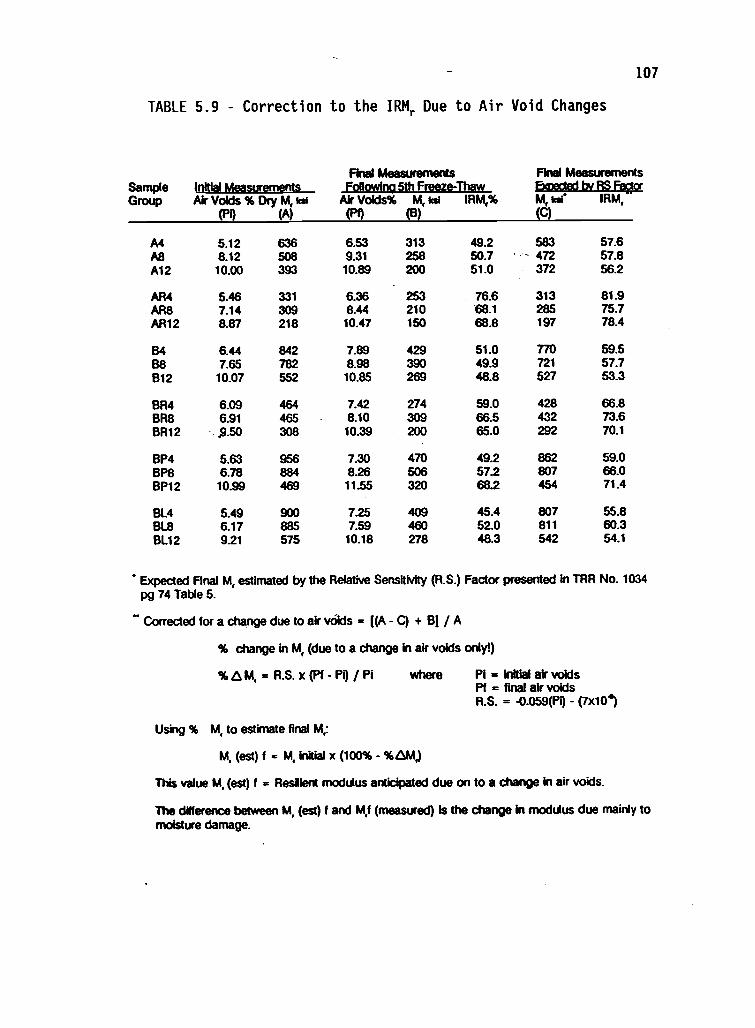
107
TABLE 5.9 Correction to the IRMr Due to Air Void Changes
SampleGroup
Initial MeasurementsFinal Measurements
Following 5th Freeze-ThawFinal Measurements6izeslatizar2figg
Air Voids % Dry M, kW(P1) (A)
Air Voids% M, ksi IRM,%
(Pt) (B)
M, IRM,(C)
A4 5.12 636 6.53 313 49.2 583 57.6A8 8.12 508 9.31 258 50.7 472 57.8Al2 10.00 393 10.89 200 51.0 372 56.2
AR4 5.46 331 6.36 253 76.6 313 81.9AR8 7.14 309 8.44 210 68.1 285 75.7AR12 8.87 218 10.47 150 68.8 197 78.4
B4 6.44 842 7.89 429 51.0 770 59.5B8 7.65 782 8.98 390 49.9 721 57.7B12 10.07 552 10.85 269 48.8 527 53.3
BR4 6.09 464 7.42 274 59.0 428 66.8BR8 6.91 465 8.10 309 66.5 432 73.6BR12 .s.50 308 10.39 200 65.0 292 70.1
BP4 5.63 956 7.30 470 49.2 862 59.0BP8 6.78 884 8.26 506 57.2 807 66.0BP12 10.99 469 11.55 320 68.2 454 71.4
BL4 5.49 900 7.25 409 45.4 807 55.8BL8 6.17 885 7.59 460 52.0 811 60.3BL12 9.21 575 10.18 278 48.3 542 54.1
Expected Final M, estimated by the Relative Sensitivity (R.S.) Factor presented in TRR No. 1034pg 74 Table 5.
Corrected for a change due to air voids = ((A - C) + B) / A
% change in M, (due to a change in air voids only!)
% R.S. x (Pf - Pi) / Pi where Pi = initial air voidsPf = final air voidsR.S. = -0.059(P) - (7x10⁴)
Using % M, to estimate final 1.4,:
M, (est) f = M, initial x (100% - %AM,)
This value AA, (est) f = Reslient modulus anticipated due on to a change in air voids.
The difference between 1.4, (est) f and M,f (measured) is the change in modulus due mainly tomoisture damage.

108
the expected IRMr of each group due only to moisture damage, and shows
a considerable amount of Mr loss following the 5th freezethaw cycle.
Following all testing and redetermination of air voids, the
samples were heated at 120°F for 15 minutes and split apart by hand.
Visual inspection of the broken specimens revealed no apparent
stripping. Figures 5.4 5.6 show typical photographs of the sample
groups. Uncoated aggregate is due only to fractured aggregate near
the faces of the specimen, most likely fractured during compaction.
From Table 5.9, it was shown that the change in IRMr due to
moisture damage exists. Because stripping was not visually evident in
the specimens, the test results did not detect stripping with respect
to the loss of adhesion. However, because there was a substantial
drop in the IRMr, the test results must imply moisture damage
associated with the loss in cohesion. This conclusion is reasonable
in that all specimens retained 4 11 grams of water after the 5th
freezethaw cycle. This retained water is believed to have either
slightly changed the phase of the asphalt or emulsified with the
asphalt, leading to a softening of the binder associated with a
reduction in cohesion.
5.5 Conclusions and Recommendations
Based on the evaluation of the study results, the following
conclusions appear warranted:
1. The test procedure developed and evaluated shows evidence
associated with moisture damage to asphalt concrete
mixtures, based on IRMr measurements and evaluation.

109
FIGURE 5.4 Typical Specimens at Low Air Void ContentsFollowing 5 FreezeThaw Cycles

110
ropummin
FIGURE 5.5 Typical Specimens at Intermediate Air Void ContentsFollowing 5 FreezeThaw Cycles

111
FIGURE 5.6 Typical Specimens at High Air Void ContentsFollowing 5 FreezeThaw Cycles

112
2. The loss in Mr associated with moisture damage was
significantly greater for the proven stripping aggregate
when compared to the proven nonstripping aggregate. The
comparison can be made following full saturation plus one
freezethaw conditioning cycle, and is valid for all levels
of air voids tested.
3. The test procedure has a high potential to differentiate
between material changes; however this study showed the AC-
20R asphalt to be the only additive to show significant
effectiveness in preventing stripping.
4. The test procedure detected partial damage to the AC
specimen that was not associated with moisture damage. This
damage was due to expansion of the specimen during the
freezing treatment.
5. The test procedure detected moistureinduced Mr loss (as
measured by the IRMr) to be the greatest for the lower air
voids groups and lowest for the higher air void groups, and
the differences were significant. This may be explained by
partial drainage of high air void groups prior to freezing.
6. The loss in Mr due to moisture damage measured by the IRMr
can be accounted for most realistically by the cohesion
mechanism theory rather than the adhesion mechanism theory.
This conclusion is based on the visual inspection of all
specimen following the 5th freezethaw cycle. Evidence of
adhesion failure was not apparent.

113
On the basis of these conclusions, it appears that the test
procedure needs modifications so as not to bias mixes based on air
void contents. It was shown that the laboratory specimen compacted to
low air void contents "stripped" significantly more than the high air
void groups. This was explained by the fact that the high air void
specimens partially drained prior to freezing, therefore the pore
water had less of a damaging effect compared with "undrained"
saturated specimen at lower air voids. The following recommendations
for the test procedure are given:
1. All saturated specimen should be frozen in a fully
submerged condition so that no drainage can take place.
Therefore, a set of saturated specimens can be placed in a
pan at least 1/2inch deeper than the height of the
specimens (suggest using a 3inch deep pan for specimens of
2.5inch height). By freezing this way, the specimens will
be confined by external forces caused by the surrounding
frozen water, which may better similate freezing
conditions of confined pavements in the field. This may
also lead to a reduction in expansion of air voids
associated with the freezing condition, which in turn led
to damage not associated with moisture damage.
2. Along these lines, it is recommended that air voids be re
determined following each conditioning cycle. This is
important to correct for damage that is not stripping. The
correction to the Mr due to air void changes in this study
was made using a sensitivity analysis presented in
Transportation Research Record 1034 (Akhter and Witczak,

114
1985). It is recommended that a similar sensitivity
analysis be performed to estimate modulus loss due to
changes in air voids over the conditioning cycles.

115
6 CONCLUSIONS AND FINAL RECOMMENDATIONS
The main goal of this study was to develop an improved test
method to quantify the moisture susceptibility of an asphalt concrete
(AC) mixture and allow a quantitative assessment of the effectiveness
of antistripping additives.
The procedure to determine stripping potential in laboratory
compacted AC specimen by means of a Repeated-Load Diametral Test
System was selected over other available alternatives because the test
is non-destructive. This reduces the total number of specimen
required by destructive tests such as the split tensile test to obtain
significant relationships between the different mixtures analyzed in
this study. A total of 108 specimen were prepared for the Primary
Factorial Study (6 replicate specimens at each of the 18 levels of
treatments ie. aggregate type, asphalt type, additive type, and air
void content). These specimens were tested for resilient modulus (Mr)
at their dry state and after each of 7 moisture conditioning cycles.
To obtain the same level of significance for comparisons made in this
study using destructive test methods, a total of 864 specimen (108
specimen x 8 cycles including dry state) would have needed to be
prepared.
The moisture-conditioning process used in this study was in
accordance with NCHRP 192 (Lottman, 1978). A partial saturation
treatment as recommended in NCHRP 274 was also used prior to full

116
saturation and freezethaw conditioning (Tunnicliff and Root, 1984).
The measurement used for comparison between treatments was the Index
of Retained Modulus (IRMr).
6.1 Conclusions
The following conclusions are drawn from the findings of the
Parametric Study and Compaction Study:
1. The Mr computed from the RepeatedLoad Diametral Test
System has a high potential to differentiate between
material changes (ie., air voids, aggregate type, and
asphalt type).
2. The test conditions that yield reliable Mr results with the
highest degree of sensitivity to material changes include:
a. 0.1 second load duration
b. 0.33 hertz load frequency
c. 50 to 60 microstrain induced diametral strain
level
3. The test temperature that yields Mr results with the
highest degree of sensitivity to material changes at the
above testing conditions is 40°F. However, temperatures up
to 60°F were found to result in values with a high degree
of sensitivity as well, and 73°F resulted in values that
were not significantly sensitive to material changes. The
highest allowable temperature is desired. The 60°F test is
practicle inside a controlled temperature box (i.e.,
refrigerator).

117
4. The preferred method of measurement using the above
developed conditions is the total Mr based on the increased
precision this measurement has over the instantaneous
measurement.
5. Based on replication of both air voids and resulting Mr
values, kneading compaction is the most desirable method of
sample preparation, although the findings of this
experiment showed that the gyratoryshear method of
compaction could be used as well. The static method and
Marshall method of compaction were ruled out because these
methods produced specimens which resulted in Mr values that
were not distinguishable between the two curing procedures
studied.
Based on the evaluation of the Primary Factorial Study, in which
the test method developed would allow for a quantifiable means to
assess moisture damage, the following conclusions appear valid:
1. The test procedure developed and evaluated shows evidence
associated with moisture damage to asphalt concrete
mixtures.
2. There is no significant difference between partial
saturation and full saturation with respect to the effect
of the IRMr.

118
3. Visual inspection of the moistureconditioned specimens
revealed that the loss in Mr associated with moisture
damage was due mainly to a loss in cohesion.
4. The results detected partial damage to the AC specimen that
was not stripping, but was due to an increase in air voids
as a result of pore water expansion during the freeze
cycle. It is very difficult to quantify the amount of
damage due to this increase in air voids.
5. The test procedure developed has good potential in
differentiating between a proven stripping aggregate and a
proven nonstripping aggregate. This differentiation can
be made following full saturation plus one freezethaw
condition cycle.
6. The test procedure has a high potential to differentiate
between material changes, and more specifically, the
effects on the IRMr of different antistripping additives
for the Baggregate, only the PaveBond Special at high air
voids appeared to be effective. The AC-20R appeared to be
a significant additive to reduce moisture damage at all air
void contents.
7. The loss in Mr due to moisture damage as measured by the
IRMr was, in general, significantly greater for the lower
air void groups as compared to higher air voids with the
same specimen constituents. The test procedure appears to
negatively bias low air void groups and positively bias
high air void groups. The bias in the procedure is

119
believed to be related to the freeze cycle used in the
conditioning process.
8. The moisture conditioning process evaluated in this study
needs modifications. The process seems to be most severe
with low air void groups, and less severe with high air
void groups. It is desirable to develop a procedure to
standardize the damage effects (i.e., control the degree of
saturation during the freeze cycle). Field performance
indicates low air void pavements are usually less effected
by moisture than are high air void pavements, therefore, a
conditioning process that does not negatively bias low air
voids is essential.
6.2 Recommendations
Based on the conclusions made on the study results, the following
recommendations for further research are given:
1. Although the test procedure developed herein has a high
potential to detect quantitatively the effects of moisture
susceptibility, it is recommended that the damage that is
not stripping also be quantitatively assessed. This type
of analysis would need to be undertaken as a future
separate study, similar to the sensitivity study by Akhter
and Witczak (1985).
2. To further reduce physical damage to the specimen that is
not stripping, it is suggested to freeze the saturated
specimen in a fully emerged distilled water bath. This

120
will guarantee full saturation at the time of freezing,
therefore, eliminating the partial drainage problem
detected in the higher air void groups. This type of
freezing may also minimize void changes associated with the
freezing pore water. The internal forces created by
freezing pore water may be neutralized by the external
forces of frozen water surrounding the specimen, leading to
minimal void volume change due to the process of one
freezethaw cycle. This idea could be checked by preparing
a reasonable number of replicate specimen (i.e., ± 1% air
voids) and subjecting half to the freezethaw used in this
study and the other half to this recommended procedure. A
comparison of air voids following a complete freezethaw
cycle should be made at the conclusion of each of five
successive cycles. If the change in voids in the proposed
method is minimal over the cycles, another study similar to
the Primary Factorial Study should be undertaken.
3. It is further recommended that the freezethaw cycle used
in this study be modified as the moisture conditioning
process used to initiate stripping. Although Lottman found
a good match in the microstructure of lab cores following
full saturation plus one freezethaw cycle with field cores
subjected only to full saturation (Lottman, 1978), the
results of lab cores do not allow for an assessment of
damage that is not stripping. The partial saturation plus
24 hour soak at 140°F, as recommended by Tunnicliff and
121
Root (1984), may lead to considerably less damage that is
not stripping, and should be investigated with the
RepeatedLoad Test System direct Mr techniques for
quantification of moisturesusceptible mixes. This method
of moisture conditioning, plus tensile strength
measurements, resulted in sensitivity to moisture damage,
effectiveness of antistripping additives and dosage of
additives, and asphalt cements from different sources
(Tunnicliff and Root, 1984). The strength loss associated
with the conditioning can only be attributed to moisture
damage by either loss of cohesion, adhesion or a
combination of both.
122
7 BIBLIOGRAPHY
AASHTO Guide for Design of Pavement Structures, American Associationof State Highway and Transportation Officials, Washington, D.C.,1986.
Akhter, G.F., and Witczak, M.W., "Sensitivity of Flexible PavementPerformance to Bituminous Mix Properties," TransportationResearch Record 1034, Transportation Research Board, Washington,D.C., 1985, p. 74.
American Society for Testing and Materials, ASTM, "Indirect TensionTest for Resilient Modulus of Bituminous Mixtures," Annual Bookof ASTM Standards, Volume 04.03, Philadelphia, PA, 1987a, pp.689-693.
American Society for Testing and Materials, ASTM, "Resistance toPlastic Flow of Bituminous Mixtures Using the MarshallApparatus," Annual Book of ASTM Standards, Volume 04.03,Philadelphia, PA, 1987b, pp. 270-273.
American Society for Testing and Materials, ASTM, "Percent Air Voidsin Compacted Dense and Open Bituminous Paving Mixtures," AnnualBook of ASTM Standards, Volume 04.03, Philadelphia, PA, 1987c,pp. 467-468.
American Society for Testing and Materials, ASTM, "Bulk SpecificGravity of Compacted Bituminous Mixtures Using Saturated Surfacedry Specimens," Annual Book of ASTM Standards, Volume 04.03,Philadelphia, PA, 1987d, pp. 407-410.
American Society for Testing and Materials, ASTM, "CompressiveStrength of Bituminous Mixtures," Annual Book of ASTM Standards,Volume 04.03, Philadelphia, PA, 1987e, pp. 238-241.
American Society for Testing and Materials, ASTM, "Preparation ofBituminous Mixture Test Specimens by Means of California KneadingCompactor," Annual Book of ASTM Standards, Volume 04.03,Philadelphia, PA, 1987f, pp. 289-293.
American Society for Testing and Materials, ASTM, "Preparation of TestSpecimens of Bituminous Mixtures by Means of Gyratory ShearCompactor," Annual Book of ASTM Standards, Volume 04.03,Philadelphia, PA, 1987g, pp. 667-672.
Coplantz, J.S., "Laboratory Test Methods to Predict Water InducedDamage to Asphalt Concrete," thesis presented the University ofNevada, at Reno, Nev., in 1987, in partial fulfillment of therequirements for the degree of Master of Science.

123
Consuegra, A., Little, D.N., and Von Quintas, H., "A ComparativeEvaluation of Laboratory Compaction Devices Based on TheirAbility to Produce Mixtures with Engineering Properties Similarto those Produced in the Field," presented at the 68th AnnualMeeting, Transportation Research Board, Washington, D.C, 1989.
Devore, Jay and Peck, Roxy, "The Analysis of Variance," StatisticsThe Exploration and Analysis of Data, West Publishing Company,St. Paul, MN, 1986a, pp. 594-600.
Devore, Jay and Peck, Roxy, "Inferences Using Two IndependentSamples," Statistics The Exploration and Analysis of Data, WestPublishing Company, St. Paul, MN, 1986b, pp. 373-374.
Dukatz, E.L.,Jr., and Phillips, R.S., "The Effect of Air Voids on theTensile Strength Ratio," Proceedings, Association of AsphaltPaving Technologists, Volume 56, 1987, pp 517-537.
Graf, P.E., "Factors Affecting Moisture Susceptibility of AsphaltConcrete Mixes," Proceedings, Association of Asphalt PavingTechnologists, Volume 55, 1986, pp. 175-212.
Hadley, W.O., Hudson, W.R., and Kennedy, T.W., "A Method of EstimatingTensile properties of Materials tested in Indirect Tension",Research Report No. 98-7, Center for Highway Research, Universityof Texas, Austin, Tex., 1970.
Heinicke, J.J., and Vinson, T.S., "Effect of Test Condition Parameterson IRMR," Journal of Transportation Engineering, Vol.114, No.2,March 1988.
Hicks, R.G., et al, "Identification and Quantification of the Extentof Asphalt Stripping in Flexible Pavements in Oregon Phase II,"Report No. FHWAOR-85-3, Materials Division, Oregon Department ofTransportation, Salem, Oregon, 1985.
Kim, K.W., Burati, J.L., and Amirkhanian, S.N., "Required Number ofSpecimens for Moisture Susceptibility Testing," presented at the68th Annual Meeting, Transportation Research Board, WashingtonD.C., 1989.
Kelly, P.B., Hicks, R.G., Furber, A.M., Vinson, T.S., "Test Method toDetermine the Degree of Stripping from Aggregates," submitted tothe U.S. DOT, March, 1986.
Kennedy, T.W., Roberts, F.L., and Lee, K.W., "Evaluation of MoistureEffects on Asphalt Concrete Mixtures," Transportation ResearchRecord 911, Transportation Research Board, Washington, D.C.,1983, pp 134-143.

124
Lottman, R.P., "Predicting MoistureInduced Damage to AsphalticConcrete," NCHRP Report 192, Transportation ResearchBoard,Washington, D.C., 1978.
Lottman, R.P., "Predicting MoistureInduced Damage to AsphalticConcreteField Evaluation," NCHRP Report 246, TransportationResearch Board, Washington, D.C., 1982.
Majidzadeh, K., and Brovold, F.N., "State of the Art: Effect of Wateron BitumenAggregate Mixtures," Highway Research Board SpecialReport 98, 1968.
Oregon Department of Transportation, Standard Specifications forHighway Construction, Section 403.11, 1984.
Petersen, Roger G., "Completely Randomized Design," Design andAnalysis of Experiments, Marcel Dekker, Inc., New York, NY,1985a, p.13.
Petersen, Roger G., "Randomized Block Design," Design and Analysis ofExperiments, Marcel Dekker, Inc., New York, NY, 1985b, pp.34-47.
Petersen, Roger G., "Factorial Experiments," Design and Analysis ofExperiments, Marcel Dekker, Inc., New York, NY, 1985c, pp.124134.
Scherocman, J.A., Mesch, K.A., and Proctor, J.J., "The Effect ofMultiple Freezethaw Cycle Conditioning on the Moisture Damage inAsphalt Concrete Mixtures," Proceedings, Association of AsphaltPaving Technologists, Volume 55, 1986, pp. 213-236.
Schmidt, R.J., and Graf, P.E., "The Effect of Water on the ResilientModulus of AsphaltTreated Mixtures," Proceedings, Association ofAsphalt Paving Technologists, Volume 41, 1972,pp. 118-147.
Scholz, T., Reitmajer, B., and Martin, K., "1986 PerformanceEvaluation Report: Lava Butte Road Fremont Junction Highway,"Transportation Research Report No. 87-27, Oregon StateUniversity, 1987.
STATGRAPHICS, Software and User's Guide, Statistical GraphicsCorporation, 1987.
Taylor, M.A., and Khosla, N.P., "Stripping of Asphalt Pavements: Stateof the Art," Transportation Research Record 911, TransportationResearch Board, Washington, D.C., 1983, pp. 150-158.
The Asphalt Institute, Mix Design Methods for Asphalt Concrete, ManualSeries Number 2, College Park, MD, May 1984.

125
Tunnicliff, 0.G., Root, R.E., "Use of Antistripping Additives inAsphaltic Concrete Mixtures Laboratory Phase," NCHRP Report274, Transportation Research Board, Washington, D.C., 1984.
Tyler, O.R., "Adhesion of Bituminous Films to Aggregates," PurdueResearch Bulletin, No. 62, Vol. 22, September, 1938.
White, T.D., "Stripping in HMA Pavements," Hot Mix Asphalt Technology,NAPA, Fall, 1987, pp 18-20.
Yoder, E.J., Witczak, M.W., Principals of Pavement Design, 2ndEdition, John Wiley and Sons, Inc., New York, N.Y., 1975.