www.SandV.com SOUND & VIBRATION/JUNE 2014 13

Test Analysis Verification Using Open Software

Teaching the topic of structural dynamics in any engineering field is a true challenge due to the wide span of the underlying subjects like mathematics, mechanics (both rigid-body and con-tinuum mechanics), numerical analysis, random data analysis and physical understanding. In this article we present a pedagogi-cal example of using experimental modal analysis to verify and calibrate a finite-element model using free, open-source software.

In an advanced subject like structural dynamics and model verification, it is advantageous to provide students with a simple case so that focus can be aimed at the theory and techniques taught, rather than object-related problems. In addition, open-source software based on Matlab® or GNU Octave, provides the advantage that students can follow each step in the process with direct access to governing equations and variables involved. The transparency offered by open software is not usually possible with commercial finite-element (FE) programs, where problems can be solved without the student understanding the underlying physics and numerical methods and their limitations.

The aim of the CALFEM® toolbox for Matlab1 (the name stands for computer-aided learning of the finite-element method) is to highlight the link between the mathematical theory and models of a phenomenon and its numerical implementation using the FE method. In such an approach, the students are motivated to fully appreciate the intimate relationship between these topics. Within such an approach, it also becomes evident for the students that many different physical problems are modeled by the same set of equations; that is, analogies exist. An additional advantage of open-source code is that the student can also copy a routine and modify it for a specific purpose, such as modeling of some special damping.

Model calibration, or correlation, theory and methods are impor-tant subjects to teach engineering students. The theory is becoming more and more important for many OEMs who require an efficient and streamlined product development process that enables get-ting products faster to the market. This is especially important in highly competitive sectors like the automotive industry. Additional efficiency, such as cost reduction in product development, may be achieved by means of reducing both the number of prototype build stages and the number of prototypes within a given build stage. Without taking correct countermeasures, it is evident that this increases the risk of product quality issues in the field due to errors in the early decision making process.

To minimize these risks, different actions need to be applied long before hardware builds take place – before and during the early phase of product development. These “front-loading” actions usually include extensive use of computer-aided technologies like CAE (computer-aided engineering) to enable improved project decision making based on objective data and engineering insight but also, which is as important, a more robust process for target-setting, including subsystem target roll-down.

A successful outcome of these actions depends heavily on the capability of applied math methods. The development of new or improved existing math methods is then an important and strategic task that needs to be done outside and ahead of regular product development work. This task also requires test and CAE communities to thoroughly co-operate to be successful. Often, organizational and conflicting priorities may be difficult barriers to overcome. Also important in math method development is to address the issue of access to hardware that matches the design. Variability due to manufacturing processes affects the hardware testing and also needs to be considered.

The lab exercise example we present in this article is based on a very simple example; a rectangular PMMA plate, similar to the so-called IES plate.2 An FE model of this plate is readily built in the popular CALFEM open-source Matlab toolbox. Experimental modal analysis is then performed, and correlation analysis and relatively simple model calibration is also completed. For the experimental modal analysis, we use the open-source ABRAVIBE toolbox, also for Matlab. If fully free, open-source software is required, all examples can be run in GNU Octave using the same toolboxes with some limitations in functionality (mainly lack-ing wireframe animation). We believe that the simplicity of this example is very advantageous. The students are allowed to focus on the process and not difficulties possessed by the structure. The FE model and the EMA measurement and analysis can be ac-complished in a matter of a few hours of lab time if the students are provided with enough information and instructions up front.

TheoryFinite-Element Model (FEM). The finite-element method for

solving structural dynamics problems is well established today in industry. More comprehensive reading concerning formulation and basic theories of FEM are found in References 3-5, while structural dynamics theory can be found in Reference 6. In the example of the PMMA plate, we use first-order shell elements. The shell elements consist of a combination of a continuous plane stress (2D) elements, which describe the membrane behavior, and structural plate ele-ments, which describe the bending behavior. Plate theory implies several simplifications and also violations of the fulfilment of solid mechanics field equations. Nevertheless, shell elements are widely used in industry due to less effort in modelling and computational efficiency. The shell elements used for this exercise are not part of the CALFEM Software but were developed and described in Refer-ence 7. Necessary command files for the CALFEM toolbox can be downloaded following the instructions at the end of this article.

In this demonstration, a simple PMMA plate with dimensions 533 ¥ 321 mm and thickness 20 mm is analyzed. The plate is similar to the so-called IES-plate proposed in Reference 2, but for practical reasons, the plate thickness was chosen slightly different from the IES-plate. A thickness of 20 mm was chosen; since it is a standard thickness in Europe. The Young’s modulus for PMMA reported in Reference 2 is 4.96 GPa, which is used as a first assumption. For the model in this case, we use the measured mass density for the actual plate (1.198 ¥ 103 kg/m3).

The baseline finite-element model, consisting of 16-by-24 ele-

Anders Brandt, University of Southern Denmark, Odense, DenmarkPer-Olof Sturesson, Volvo Car Corp., SwedenMatti Ristinmaa, Lund University, Sweden

Figure 1. Finite-element model with 384 elements, 425 nodes.

www.SandV.com14 SOUND & VIBRATION/JUNE 2014

ments with a total of 425 DOFs, is shown in Figure 1. This mesh was chosen because it can easily be reduced to the 5-by-7 mesh, which will be used for the experiment. To assess the accuracy of the chosen mesh, two alternative meshes, one coarser and one more detailed, were also tried, For each of the three meshes, the 10 lowest normal modes were computed.

The results of these runs (Table 1) show that there is some in-creased stiffness for the coarser models, resulting in slightly higher eigen frequencies. The middle grid density seems reasonable, however, so we decided to use this model.

In CALFEM, the following steps were implemented in this demonstration example:1. Generate geometrical topology (nodes).2. Generate element to nodal degree of freedom topology.3. For each element, calculate mass and stiffness matrices, and

assemble the data into global matrices.4. Solve the set of equations (eigenvalue solution for normal

modes).5. Post-process the results.

Experimental Modal Analysis (EMA). Experimental modal analysis is based on measurements of frequency response functions from which the modal parameters (natural frequencies, relative damping ratios, and mode shapes) are extracted using the relation:

where [H(f)] is the matrix of frequency responses in receptance form (displacement/force), Qr is the modal scaling constant, sr is the pole of mode number r, {y}r is the mode shape vector for mode number r, and N is the number of modes (number of degrees of freedom). In the typical case, a few references R are used. The use of fixed shakers and roving response sensors (usually accelerometers)leads to estimates of R columns from the matrix in Eq. 1. Another method is to let R reference accelerometers be fixed and roving the force around, usually with an impact hammer. This leads to estimates of R rows of Eq. 1. Since the frequency response matrix is symmetric, it can easily be transposed if the latter strategy was chosen, so that the formulation may be implemented only for the case of fixed-force references.

Instead of the frequency domain relation in Eq. 1, time domain methods extract the modal parameters by using the relationship of the impulse responses in a matrix [h(t)], which can be expressed as:

If two or more poles are very close, several references usually have to be used to correctly extract the corresponding mode shapes. Also, many times the complex conjugate poles and mode shapes are included in the numbering for simplicity so that the sums go from 1 to 2N and only include one term. Eq. 2 can then be rewritten as:

where [y] is the mode shape matrix with mode shapes in its col-umns, es trÈÎ ˘̊ is a diagonal matrix with the complex exponential terms, and [L] is a matrix with modal participation factors.

A common family of parameter extraction methods for extracting poles are the complex exponential methods; the prony method8, the least-squares complex exponential method9, and the polyrefer-ence time domain method.10 The latter method can handle closely coupled poles. In all cases, the mode shapes are usually computed in a second step, for example by the least-squares frequency domain method.11 These methods are all implemented in the ABRAVIBE toolbox,12 and theory and practice of its use for EMA can be found in Reference 13.

Model Verification. There are two common methods to verify an FE model, either using natural frequencies and mode shapes, or using frequency responses.14 In this article, we use the former method. The first comparison is usually to match frequencies of each mode in the FE model with the corresponding mode in the experimental results. For this comparison, the MAC (modal assur-

ance criterion) matrix15 is used to determine which mode in one set should be paired with a mode in the other set. The MAC value between two modes r and s is a number between 0 and 1, defined by:

and is similar to the correlation coefficient of the two vectors. For best comparison between the test and analytical models, a good EMA test for verification purposes should use sensor positions that minimize the off-diagonal components in the MAC matrix. It was concluded in Reference 2 that the 5 × 7 grid used for the IES plate fulfills this criterion.

After pairing the mode shapes and comparing the natural fre-quencies of the EMA results with the eigenfrequencies of the FE model, the FE model should be modified so that eigenfrequencies match the experimental model within some accuracy limits. If test errors are evident, the test sequence should be reworked. Recom-mended criteria for a verified FE model is that the eigenfrequencies for most important modes lie within 2-10%, the diagonal elements of the MAC matrix are greater than 0.9 and off-diagonal elements are less than 0.1.14

For simple structures like the example used in this article, the upper limit of frequency criteria should be less than 5%, and the diagonal elements of the MAC matrix should be greater than 0.95. In practice for complex engineering FE models, using too stringent correlation criteria provides limited additional benefits but adds time and cost. In this simple example, parameters to be adjusted are the material properties like the Young’s modulus used in the FE model.

More advanced verifications could now be done. To find local errors in the FE model, the cross-orthogonality matrix14 can be used. This requires computing a reduced mass matrix and will not be done in the current example. The CoMAC (coordinate MAC)16 can also be used for this purpose. This measure is defined for each DOF q by:

That is, a summation of the correlation coefficients of each DOF over all modes. A CoMAC value different from unity reveals a DOF where there is discrepancy between the FE model mode shapes and the experimental mode shapes. This could be due to problems in the FE model, where sometimes local stiffnesses of the structure can be hard to model correctly. But a low CoMAC value can also be due to a local error in the EMA result, so great care must be taken when interpreting local discrepancies.

Simple Plate ResultsFE Results. The first 10 eigenfrequencies from a normal mode

solution of the FE model with the mid grid density in Table 1 are shown in Table 2 along with corresponding values from the EMA test. For the sake of simplicity, the modes are arranged in the order of the experimental modal analysis. So the first two FE modes have

Table 1. List of eigenfrequencies (Hz) from normal mode solution of FE models with three different meshes.

Mesh 1 Mesh 2 Mesh 3 Mode (7 ¥ 11) (16 ¥ 24) (34 ¥ 49) 1 145.2 145.3 145.5 2 150.0 150.3 150.4 3 340.7 340.5 340.4 4 403.8 401.5 401.0 5 412.8 413.4 413.5 6 522.3 522.0 521.8 7 620.0 616.4 615.3 8 752.5 751.7 750.9 9 846.6 827.5 823.1 10 1002.5 1005.7 1001.4

H fQ

s

Q

sr r r

T

r

r r r

T

rr

N

( )ÈÎ ˘̊ ={ } { }

-+

{ } { }-=

Ây yw

y y

wj j

* * *

*1

(1)

(2)h t Q e Q er r r

T s tr r r

T s t

r

Nr r( )ÈÎ ˘̊ = { } { } + { } { }

=Â y y y y* * * *

1

(3)h t e Ls tr( )ÈÎ ˘̊ = [ ]ÈÎ ˘̊[ ]Y

MAC ,r sr

T

s

r

T

r s

T

s

( ) ={ } { }

{ } { } { } { }y y

y y y y

2

(4)

(5)Cq

qr fe qrr

N

qrr

N

fe qrr

N=

ÊËÁ

ˆ¯̃=

= =

Â

 Â

( )( )

( ) ( )

exp

exp

y y

y y

1

2

2

1

2

1

www.SandV.com SOUND & VIBRATION/JUNE 2014 15

been swapped, since they appeared in the opposite order. This may be due to the fact that the shell element formulation yields too high a bending stiffness. Application of more advanced plate theory could address this.

EMA Results. Experimental modal analysis was conducted by impact excitation using two reference accelerometers in two corners along one of the long axes of the plate. A 7 × 5 grid was used for the measurements. The structure was suspended using soft rubber cords, which yielded rigid-body modes below 5 Hz. Time-domain signals were recorded and processed as described in References 15 and 17. An example FRF and corresponding co-herence function are shown in Figure 2, where the coherence is very close to unity. Shaker excitation is an alternative that could be used with similar results. An advantage with the PMMA plate for teaching purposes is that it is relatively easy to measure with good accuracy with any type of excitation.

The polyreference time domain method10,17 was used for esti-mating the poles, followed by a computation of the mode shapes using the frequency domain least-squares method, in both cases using available functions in the ABRAVIBE toolbox. This resulted in a stabilization diagram as shown in Figure 3, where also an example of a synthesized versus a measured FRF plot is shown. The results of the experimental modal analysis are shown in Table 2, where the first 10 modes are tabulated in the third column. It is relatively easy to successfully obtain at least 20 experimental modes, but for correlation with the FE model, it is more realistic to select the 10 lowest modes. As follows from Table 2, the 10 lowest undamped natural frequencies range from approximately 145 to 993 Hz. Relative damping ratios range from 2.1% to 3.2% and are tabulated in column five of Table 2.

FE Model VerificationComparison of the analytical and experimental results in Table

2 shows that the frequencies are relatively close and that the two first modes appear in opposite order in the FE model solution

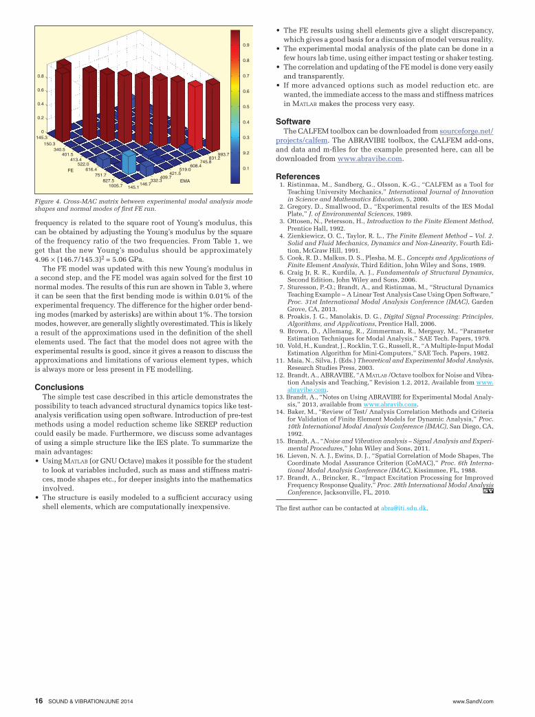
compared to the experiment. For comparison with the experimental mode shapes, the mode shapes from the normal mode solution were reduced to every fourth DOF, corresponding to the 5 × 7 grid used for the experiment. A computation of the cross-MAC matrix showed that the mode shapes were very similar, with MAC values in excess of 0.97, except for Mode 9, where the MAC matrix was 0.92. A plot of the cross-MAC is shown in Figure 4.

FE Model CalibrationA simple modification of the FE model to calibrate it with

the EMA test results is to match the frequency of the first bend-ing mode of the FE model with the corresponding frequency from the experimental results. Since the first bending mode

Figure 2. Example FRF (a) and coherence function (b) for the Plexiglas plate; plotted FRF is a driving point, i.e. the force and acceleration are both in the same point (DOF 1).

Table 2. Finite-element eigenfrequencies, experimentally obtained undamped natural frequencies and relative damping coefficients from experimental modal analysis of PMMA plate, and relative difference between frequencies.

EMA FE Exp. Natural Mode Mode Eigenfreq. Freq., Hz Diff., % Damp, % Description 1 150.3 145.1 3.5 3.20 First torsion 2 145.3 146.7 –0.96 2.85 First bending, x 3 340.5 332.3 2.4 2.59 Second torsion 4 401.5 409.7 –2.0 2.48 Second bending, x 5 413.4 421.5 –1.9 2.46 First bending, y 6 522.0 519.0 0.6 2.32 Higher order 7 616.4 608.4 1.3 2.36 Higher order 8 751.7 745.8 0.8 2.23 Higher order 9 827.5 831.2 –0.4 2.16 Third bending, x 10 1005.7 993.7 1.2 2.21 Higher order

Table 3. List of eigenfrequencies of FE model after modifying Young’s modulus and undamped natiural frequencies from experimebtal modal analysis.

Natural Frequency, Hz Mode FE Model EMA Difference, % 1 151.8 145.1 4.40 2 146.7 146.7 0.01* 3 343.8 332.3 3.35 4 405.4 409.7 −1.06* 5 417.4 421.5 −0.98* 6 527.0 519.0 1.52 7 622.3 608.4 2.24 8 759.0 745.8 1.73 9 835.4 831.2 0.51* 10 1015.4 993.7 2.13

* Bending modes, which are relatively well modeled; frequencies of torsion modes are typically overestimated by shell elements.

Figure 3. Stabilization diagram overlaid by multivariate mode indicator functions (a) and an example of measured vs. synthesized FRF (b).

Select polesthen <RETURN)

Num

ber o

f Pol

es

60

50

40

30

20

20

0200 300 400 500 600 700 800 900 1000 Frequency, Hz

(a)

100

101

100

10–1

10–2

100 200 300 400 500 600 700 800 900 1000 1100 Frequency, Hz

Acce

lera

tion,

(m/s

)2 /N

MeasuredSynthesized

(b)

101

100

10–1

10–2

1.0

0.9

0.8

0.7

0.6

0.5

(a)

(b)

0 100 200 300 400 500 600 700 800 900 1000 Frequency, Hz

Coh

eren

ce

F

RF,

(m/s

2 )/N

www.SandV.com16 SOUND & VIBRATION/JUNE 2014

• The FE results using shell elements give a slight discrepancy, which gives a good basis for a discussion of model versus reality.

• The experimental modal analysis of the plate can be done in a few hours lab time, using either impact testing or shaker testing.

• The correlation and updating of the FE model is done very easily and transparently.

• If more advanced options such as model reduction etc. are wanted, the immediate access to the mass and stiffness matrices in Matlab makes the process very easy.

SoftwareThe CALFEM toolbox can be downloaded from sourceforge.net/

projects/calfem. The ABRAVIBE toolbox, the CALFEM add-ons, and data and m-files for the example presented here, can all be downloaded from www.abravibe.com.

References 1. Ristinmaa, M., Sandberg, G., Olsson, K.-G., “CALFEM as a Tool for

Teaching University Mechanics,” International Journal of Innovation in Science and Mathematics Education, 5, 2000.

2. Gregory, D., Smallwood, D., “Experimental results of the IES Modal Plate,” J. of Environmental Sciences, 1989.

3. Ottosen, N., Petersson, H., Introduction to the Finite Element Method, Prentice Hall, 1992.

4. Zienkiewicz, O. C., Taylor, R. L., The Finite Element Method – Vol. 2. Solid and Fluid Mechanics, Dynamics and Non-Linearity, Fourth Edi-tion, McGraw Hill, 1991.

5. Cook, R. D., Malkus, D. S., Plesha, M. E., Concepts and Applications of Finite Element Analysis, Third Edition, John Wiley and Sons, 1989.

6. Craig Jr, R. R., Kurdila, A. J., Fundamentals of Structural Dynamics, Second Edition, John Wiley and Sons, 2006.

7. Sturesson, P.-O.; Brandt, A., and Ristinmaa, M., “Structural Dynamics Teaching Example − A Linear Test Analysis Case Using Open Software,” Proc. 31st International Modal Analysis Conference (IMAC), Garden Grove, CA, 2013.

8. Proakis, J. G., Manolakis, D. G., Digital Signal Processing: Principles, Algorithms, and Applications, Prentice Hall, 2006.

9. Brown, D., Allemang, R., Zimmerman, R., Mergeay, M., “Parameter Estimation Techniques for Modal Analysis,” SAE Tech. Papers, 1979.

10. Vold, H., Kundrat, J., Rocklin, T. G., Russell, R., “A Multiple-Input Modal Estimation Algorithm for Mini-Computers,” SAE Tech. Papers, 1982.

1 1. Maia, N., Silva, J. (Eds.) Theoretical and Experimental Modal Analysis, Research Studies Press, 2003.

12. Brandt, A., ABRAVIBE, “A Matlab /Octave toolbox for Noise and Vibra-tion Analysis and Teaching,” Revision 1.2, 2012, Available from www.abravibe.com.

13. Brandt, A., “Notes on Using ABRAVIBE for Experimental Modal Analy-sis,” 2013, available from www.abravib.com.

14. Baker, M., “Review of Test/ Analysis Correlation Methods and Criteria for Validation of Finite Element Models for Dynamic Analysis,” Proc. 10th International Modal Analysis Conference (IMAC), San Diego, CA, 1992.

15. Brandt, A., “Noise and Vibration analysis – Signal Analysis and Experi-mental Procedures,” John Wiley and Sons, 2011.

16. Lieven, N. A. J., Ewins, D. J., “Spatial Correlation of Mode Shapes, The Coordinate Modal Assurance Criterion (CoMAC),” Proc. 6th Interna-tional Modal Analysis Conference (IMAC), Kissimmee, FL, 1988.

17. Brandt, A., Brincker, R., “Impact Excitation Processing for Improved Frequency Response Quality,” Proc. 28th International Modal Analysis Conference, Jacksonville, FL, 2010.

frequency is related to the square root of Young’s modulus, this can be obtained by adjusting the Young’s modulus by the square of the frequency ratio of the two frequencies. From Table 1, we get that the new Young’s modulus should be approximately 4.96 ¥ (146.7/145.3)2 = 5.06 GPa.

The FE model was updated with this new Young’s modulus in a second step, and the FE model was again solved for the first 10 normal modes. The results of this run are shown in Table 3, where it can be seen that the first bending mode is within 0.01% of the experimental frequency. The difference for the higher order bend-ing modes (marked by asterisks) are within about 1%. The torsion modes, however, are generally slightly overestimated. This is likely a result of the approximations used in the definition of the shell elements used. The fact that the model does not agree with the experimental results is good, since it gives a reason to discuss the approximations and limitations of various element types, which is always more or less present in FE modelling.

ConclusionsThe simple test case described in this article demonstrates the

possibility to teach advanced structural dynamics topics like test-analysis verification using open software. Introduction of pre-test methods using a model reduction scheme like SEREP reduction could easily be made. Furthermore, we discuss some advantages of using a simple structure like the IES plate. To summarize the main advantages:• Using Matlab (or GNU Octave) makes it possible for the student

to look at variables included, such as mass and stiffness matri-ces, mode shapes etc., for deeper insights into the mathematics involved.

• The structure is easily modeled to a sufficient accuracy using shell elements, which are computationally inexpensive.

Figure 4. Cross-MAC matrix between experimental modal analysis mode shapes and normal modes of first FE run.

0.9

0.8

0.7

0.6

0.5

0.4

0.3

9.2

0.1

0.8

0.6

0.4

0.2

0145.3

150.3340.5

401.5413.4

522.0616.4

751.7827.5

1005.7 145.1146.7

332.3409.7

421.5519.0

608.4745.8

831.2993.7

FE

EMA

The first author can be contacted at abra@iti.sdu.dk.