L

I II

PCO2 =

76 mmHg

PCO2 = 456 mmHg

d

Molecular Diffusion in Gases

Molecular Diffusion of Helium in Nitrogen Example 6.1-1, page 413

A mixture of He and N2 gas is contained in a pipe at 298K and 1.0atm total pressure which is

constant throughout. At one end of the pipe at point 1, the partial pressure PA1 of He is 0.60atm

and at the other end 0.2m, PA2 is 0.20 atm. Calculate the flux of He at steady state if DAB is

0.687 x 10-4

m2/s.

PA1 = 0.6 atm

PA2 = 0.2 atm

P = 1 atm

R = 82.057 m3 atm/kgmol K

T = 298K

z2-z1 = 0.2m

DAB = 0.687 x 10-4

m2/s

DAB for a gas is constant; P is constant meaning C is also constant; flux is constant at steady

state.

Flux,

12

21

zz

CCDJ AAAB

AZ

if C = P/RT

12

21

zzRT

PPDJ AAAB

AZ

Substitute in values:

64

1063.52.0298057.82

2.06.010687.0

AXJ kgmol/m2s

Equimolar Counterdiffusion Example 6.2-1, page 415

Ammonia gas (A) is diffusing through a uniform tube 0.10m

long containing N2 gas (B) at 1.0132x105 Pa pressure and

298K. At point 1, PA1 = 1.013x104 Pa and at point 2,

PA2 = 0.507x104 Pa. DAB = 0.230x10

-4 m

2/s.

Calculate the flux J*

A and J*

B at steady state.

PA1 = 1.013x104 Pa

PA2 = 0.507x104 Pa

DAB = 0.230x10-4

m2/s

T = 298K

P = 1.0132x105 Pa

z2 – z1 = 0.10 m

R = 8314.3 m3 Pa/kgmol K

7444

12

21 1070.41.02983.8314

10507.010013.110230.0

zzRT

PPDJ AAAB

AZ kgmol A/m2 s

H2O

Diffusion of Water Through Stagnant, Nondiffusing Air Example 6.2-2 page 419

Water in the bottom of a narrow metal tube is held at a constant

temperature of 293K. The total pressure of air (assumed dry) is

1.01325x105 Pa (1.0atm) and the temperature is 293K.

Water evaporates and diffuses through the air in the tube,

and the diffusion path z2 – z1 is 0.1524 m long. Calculate the

rate of evaporation at steady state. The diffusivity of water vapor at 293K and 1 atm is

0.250x10-4

m2/s. Assume that the system is isothermal.

P = 1.01325x105 Pa = 1.0 atm

T = 293K

z2 – z1 = 0.1524m

DAB = 0.250x10-4

m2/s

Vapor pressure of water, PA1 = 0.0231 atm

Water pressure in dry air, PA2 = 0 atm

R = 82.057 m3 atm/kgmol K

988.0

0231.01

01ln

0231.0101

ln1

2

12

B

B

BBBM

P

P

PPP atm

21

12

AA

BM

ABA PP

PzzRT

PDN

74

10595.100231.0988.01524.0293057.82

0.110250.0

AN kgmol/m2s

Diffusion in a Tube with Change in Path Length Example 6.2-3, page 419

Water in the bottom of a narrow metal tube is held at a constant temperature of 293K. The total pressure of air

(assumed dry) is 1.01325x105 Pa (1.0atm) and the temperature is 293K. At a given time, t, the level is z meters from

the top. As water vapor diffuses through the air, the level drops slowly. Derive the equation for the time tF for the

level to drop from a starting point of zo m at t = 0 and zF at t = tF seconds.

We can assume a pseudo-steady state condition because the level drops slowly. Now, both NA

and z are variables.

21

12

AA

BM

ABA PP

PzzRT

PDN

Assuming a cross-sectional area of 1 m2, the level drops dt in dz seconds, and the leftover kgmol

of A is PAdz/MA:

dtM

dzN

A

AA

11

Rearranging and integrating:

FF t

AA

BM

ABz

zA

A dtPPRTP

PDzdz

M 021

0

21

2

0

2

2 AAABA

BMFA

FPPPDM

RTPzzt

Stagnant B

r2

Diffusing

A

r1

Diffusion Through a Varying Cross-Sectional Area – Evaporation Derivation

HW1.1 In the lecture we showed that the molar rate of material A evaporating from a spherical

drop immersed in material B could be written as

2,

1,

21

ln11

4 A

AABA

pP

pP

RT

PD

rr

N

where

AN is the molar rate of material A leaving

the drop

r1 and r2 are two radial points away from

the sphere center

DAB is the diffusion coefficient P is the total

system pressure

R is the ideal gas constant

T is the system temperature

pA,1 is the partial pressure of A at point 1

pA,2 is the partial pressure of A at point 2

Starting with this equation, derive the following approximate equation for the molar flux at the particle

surface, NA,1

2,1,

1

1,

2AA

ABA cc

D

DN

where D1 is the diameter of the spherical drop

cA,1 is the molar concentration of material A at the surface of the drop

cA,2 is the molar concentration of material A far from the drop

Assume point 1 is at the drop’s surface

Assume point 2 is very far away from the drop, so r2 >> r1

1

2

21

ln11

4 A

AABA

PP

PP

RT

PD

rr

N

1

2

1

ln4 A

AABA

PP

PP

RT

PD

r

N

Now multiply the equation by 1/r1, rewrite the radius as 2/D on the right

side, substitute for surface flux, NAs, and PBM:

1

2

21

1

2

12

lnlnA

A

AA

B

B

BBBM

PPPP

PP

PP

PPP and

2

14 r

NN A

AS

So we rewrite the equation as: BM

AAABAS

P

PP

DRT

DN 212

Assume low vapor pressure, so PA1, PA2 << P and use a Taylor Series approximation ln(x) = x-1:

1

2

A

A

PP

PPis approaching 1, so 1ln

1

2

1

2

A

A

A

A

PP

PP

PP

PP

Now,

P

PP

PP

PP

PP

PPPP AA

A

AA

A

AA 21

1

21

1

12

so PBM ≈ P.

Lastly, PA1 = CA1RT and PA2 = CA2RT:

212121

222AA

ABAA

ABAA

BM

ABAS CC

D

DRTCRTC

RTD

DPP

P

P

RTD

DN

where CA1 = concentration at surface of the drop and CA2 = concentration far from the drop ≈ 0

Evaporation of a Napthalene Sphere Example 6.2-4, page 421

A sphere of naphthalene having a radius of 2.0mm is suspended in a large volume of still air at 318K

and 1.01325x105 Pa (1.0atm). The surface temperature of the naphthalene can be assumed to be at

318K and its vapor pressure at 318K is 0.555 mmHg. The DAB of naphthalene in air at 318K is

6.92x10-6

m2/s. Calculate the rate of evaporation of naphthalene from the surface.

r = 2.0mm

T = 318K

P = 1.01325x105 Pa

DAB = 6.92x10-6

m2/s

Vapor pressure, PA1 = 0.555 mmHg = 74 Pa

PA2 = 0 Pa

R = 8314.3 m3 Pa/kgmol K

5

5

5

55

1

2

12 100129.1

74101.01325

0101.01325ln

74101.013250101.01325

ln

B

B

BBBM

P

P

PPP Pa

8

5

56

21

01

1068.9100129.1002.03183.8314

1001325.11092.6

AA

BM

ABA PP

PrrRT

PDN kgmol A/m

2s

6.2-5.) Mass Transfer from a Napthalene Sphere to Air

Mass transfer is occurring from a sphere of naphthalene having a radius of 10mm. The sphere is in a

large volume of still air at 52.6ºC and 1atm absolute pressure. The vapor pressure of naphthalene at

52.6ºC is 1.0 mmHg. The diffusivity of naphthalene in air at 0ºC is 5.16 x 10-6

m2/s. Calculate the rate

of evaporation of naphthalene from the surface in kg mol/s m2. [Note: the diffusivity can be corrected

for temperature by using the temperature correction factor from the Fuller et al. equation (6.2-45)]

Assumptions:

the system is at steady-state, so the radius of the sphere is not changing

point 1 is at the surface of the sphere and point 2 is very far away , so r2 >> r1

R = 8314 m3 Pa/kgmol K

T = 325.75 K

r = 0.01 m

PA1=(1.0mmHg)(1.01325 x 105

Pa/760 mmHg) =

133.322 Pa

PA2 = 0 Pa because the air is still

First calculate DAB at the new temperature:

DAB(52.6ºC) = DAB(0ºC)

1

1

2

75.1

1

2

P

P

T

T= (5.16 x 10

-6 m

2/s)(325.75/273.15)

1.75 = 7.023 x 10

-6

m2/s

Now solve for AN :

1

2

21

ln11

4 A

AABA

PP

PP

RT

PD

rr

N

1

2

1

ln4 A

AABA

PP

PP

RT

PD

r

N

01001325.1

322.1331001325.1ln

75.3258314

1001325.110023.7

1.04 5

556

AN

= 4.34736 x 10-11

kgmol/s

Now solve for NA = AN /A = (4.34736 x 10-11

kgmol/s)/(4πr12) = 3.46 x 10

-8 kgmol/m

2s

6.2-9 Time to Completely Evaporate a Sphere A drop of liquid toluene is kept at a uniform temperature of 25.9ºC and is suspended in air by a

fine wire. The initial radius r1 = 2.00mm. The vapor pressure of toluene at 25.9ºC is PA1 = 3.84

kPa and the density of liquid toluene is 866 kg/m3.

(a) Derive Eq. (6.2-34) to predict the time tF for the drop to evaporate completely in a large

volume of still air. Show all steps.

(b) Calculate the time in seconds for complete evaporation.

(a) Equations for flux:

BM

AAABA

P

PP

RTr

PD

r

N 21

24

and

dtM

dVN

A

AA

Volume of the sphere, 3

34 rV so the derivative of volume is: 24 r

dr

dV

Plug this volume derivative into molar flux equation for dV:

dtM

drrN

A

AA

24

Now set AN equal in each equation:

BM

AAAB

A

A

P

PP

RTr

PD

rdtM

drr 21

2

2

4

14

Separate variables and integrate both sides:

r

AAABA

BMAt

rdrPPPDM

PRTdt

021

0

21

2

2 AAABA

BMA

PPPDM

PRTrt

(b) Now use the equation to find the time in seconds:

PA1 = 3840 Pa

PA2 = 0 Pa

P = 1.01325 x 105 Pa

MA = 92.14 kg/kgmol

DAB = 0.86 x 10-4

m2/s

R = 8314 m3 Pa/kgmol K

T = 299.05 K

ρ = 866 kg/m3

r1 = 0.002 m

Solve for PBM:

1

2

21

lnA

A

AABM

PPPP

PPP = 99392.6 Pa

tevap = 21

2

2 AAABA

BMA

PPPDM

PRTr

=

0384010086.014.922

6.9939205.2998314002.08664

2

1388.23 seconds

6.2-10 Diffusion in a Nonuniform Cross-Sectional Area – Changing Pipe Diameter

The gas ammonia (A) is diffusing at steady state through N2 (B) by equimolar counterdiffusion in a conduit

1.22m long at 25ºC and a total pressure of 101.32 kPa abs. The partial pressure of ammonia at the left end

is 25.33 kPa and at the other end is 5.066 kPa. The cross section of the conduit is in the shape of an

equilateral triangle, the length of each side of the triangle being 0.0610m at the left end and tapering

1.22m

.0305m .061m

uniformly to 0.0305m at the right end. Calculate the molar flux of ammonia. The diffusivity is DAB = 0.230 x

10-4

m2/s.

Area = tan4

1 2b (60º)

To find an equation for how b changes with the length, create a linear fit based on two points:

At the first end: (0, 0.061) and at the other end: (1.22, 0.0305)

Slope = -0.0305/1.22 = -0.025

b = -0.025L + 0.061

So now Area = tan061.0025.04

1 2 L (60º) = 0.000271 L

2 – 0.001321 L + 0.001611

dL

dP

RT

D

A

N AABA

dL

dP

RT

DN AABA

0.001611 L 0.001321 - L 0.000271 2

Now separate and integrate both sides:

2

1

22.1

0 2 0.001611 L 0.001321 - L 0.000271

PA

PAA

ABA dPRT

DdL

N

PA1 = 25.33 kPa

PA2 = 5.066 kPa

DAB = 0.230 x 10-4

m2/s

R = 8314 m3 Pa/kgmol K

T = 298.15 K

Now plug into integrate equation:

15.2988314

25330506610230.08.1514

4

12

RT

PPDN AAAB

A AN = 1.24 x 10-10

kgmol/s

Now solve for NA:

NA = AN /A = 60tan0610.0025.0

41

1024.12

10

L at any point along the length, L

Molecular Diffusion in Liquids

Diffusion of Ethanol (A) Through Water (B) Example 6.3-1, page 429

An ethanol(A)-water(B) solution in the form of a stagnant film 2.0mm thick at 293K is in contact at one

surface with an organic solvent in which ethanol is soluble and water is insoluble. Hence, NB = 0. At

point 1, the concentration of ethanol is 16.8 wt % and the solution density is ρ1 = 972.8 kg/m3. At

point 2, the concentration of ethanol is 6.8 wt % and ρ2 = 988.1 kg/m3. The diffusivity of ethanol is

0.740x10-9

m2/s. Calculate the steady-state flux NA.

DAB = 0.740x10-9

m2/s

T = 293K

CA1 = 16.8

CA2 = 6.8

ρ1 = 972.8 kg/m3

ρ2 = 988.1 kg/m3

Meth =46.05

Mwater = 18.02

Calculate the mole fractions, taking a basis of 100 kg:

0732.0

02.182.83

05.468.16

05.468.16

1

AX 0277.0

02.182.93

05.468.6

05.468.6

2

AX

9268.00732.011 11 AB XX 9723.00277.011 22 AB XX

Now calculate the molecular weight:

07.20

02.182.83

05.468.16

1001

kgM kg/kgmol 75.18

02.182.93

05.468.6

1001

kgM kg/kgmol

Now calculate CAvg:

6.502

75.18/1.98807.20/8.972

2

// 2211

MM

Cavg

kgmol/m

3

949.0

9723.0

9268.0ln

9268.09723.0

ln1

2

12

B

B

BBBM

X

X

XXX

79

21

12

1099.8949.0002.0

0277.00732.06.5010740.0

AA

BM

avgAB

A xxxzz

CDN kgmol/m

2s

6.3-2 Diffusion of Ammonia in an Aqueous Solution An ammonia (A) – water (B) solution at 278K and 4.0mm thick is in contact at one surface with an organic

liquid at this interface. The concentration of ammonia in the organic phase is held constant and is such that

the equilibrium concentration of ammonia in the water at this surface is 2.0 wt % ammonia (density of

aqueous solution 991.7 kg/m3) and the concentration of ammonia in water at the other end of the film 4.0

mm away is 10 wt% (density = 961.7 kg/m3). Water and the organic are insoluble in each other. The

diffusion coefficient of ammonia in water is 1.24 x 10-9

m2/s.

(a) At steady state, calculate the flux NA in kg mol/s m2

(b) Calculate the flux NB. Explain.

(a)

ρ1 = 991.7 kg/m3

ρ2 = 961.7 kg/m3

M1 = 17.9806 kg/kgmol

M2 = 17.9031 kg/kgmol

T = 278 K

CA1 = 0.02

CA2 = 0.1

z1 = 0.004 m

z2 = 0 m

Calculate Cavg:

9031.17

7.961

9806.17

7.991

2

1

2

1

2

2

1

1

MMCavg

54.435 kgmol/m

3

Calculate XBM:

Xw1 = 1-0.02 = 0.98

Xw2 = 1-0.1 = 0.9

98.0/9.0ln

98.09.0

ln 12

12

BB

BBBM

XX

XXX 0.939432

Now calculate flux:

BM

AAavgAB

AXzz

XXCDN

12

21

=

939432.0004.00

1.002.0435.541024.1 9

= 1.437 x 10-6

kgmol/m2 s

Prediction of Diffusivities in Liquids Prediction of Liquid Diffusivity Example 6.3-2, page 432

Predict the diffusion coefficient of acetone in water at 25ºC and 50ºC using the Wilke-Chang equation. The

experimental value 1.28x10-9

m2/s at 298K.

From Appendix A.2, the viscosity of water at 25ºC is μB = 0.8937 x 10-3

Pa s and at 50ºC is 0.5494 x 10-3

Pa

s. From Table 6.3-2 for CH3COCH3 with 3 carbons + 6 hydrogens + 1 oxygen.

VA = 3(0.0148) + 6(0.0037) + 1(0.0074) = 0.0740 m3 kgmol

For the water association parameter φ = 2.6 and MB = 18.02 kg mass/kgmol. For 25ºC:

9

6.0

2/116

6.0

2/116 10277.10740.08937.0

29802.186.210173.110173.1

AB

BABV

TMD

m

2/s

For 50ºC:

9

6.0

2/116

6.0

2/116 10251.20740.05494.0

32302.186.210173.110173.1

AB

BABV

TMD

m

2/s

Prediction of Diffusivities of Electrolytes in Liquids Diffusivities of Electrolytes Example 6.3-3, page 434

Predict the diffusion coefficients of dilute electrolytes for the following cases:

(a) For KCl at 25ºC, predict DºAB and compare with the value in Table 6.3-1

(b) Predict the value of KCl at 18.5ºC. The experimental value is 1.7x10-5

cm2/s

(c) For CaCl2 predict DAB at 25ºC. Compare with the experimental value of 1.32x10-5

cm2/s; also,

predict Di of the ion Ca2+

and of Cl- and use Eq. 6.3-12

(a) From Table 6.3-3, λ+ (K+) = 73.5 and λ- (Cl

-) = 76.3:

51010 10993.1

3.76/15.73/1

1/11/129810928.8

/1/1

/1/110928.8

nnTDAB

cm2/s

(b) To change the temperature, we use a simple correction factor:

T = 18.5ºC = 291.7K

From Table A.2-4, μw = 1.042 cP

55 10671.1042.1

7.29110993.1

334255.18

w

ABAB

TDD

cm

2/s

(c) From Table 6.3-3, λ+ (Ca2+

/2) = 59.5 and λ- (Cl-) = 76.3, n+ = 2 and n- = 1:

577 10792.02

5.5910662.210662.22

nD

Ca

cm

2/s

577 10031.21

3.7610662.210662.2

nD

Cl

cm

2/s

5

5510335.1

10031.2/110792.0/2

12

//

DnDn

nnDAB

cm2/s

Molecular Diffusion in Biological Solutions and Gels

Prediction of Diffusivity of Albumin Example 6.4-1, page 438

Predict the diffusivity of bovine serum albumin at 298K in water as a dilute solution using the modified

Polson equation (6.4-1).

T = 298 K

MA = 67500 kg/kgmol from Table 6.4-1 (pg 437)

μwater = 0.8937x10-3

Pa s

We can use the equation for the prediction of diffusivities for biological solutes:

11

3/13

15

3/1

15

1070.767500108937.0

2981040.91040.9

A

ABM

TD

m

2/s

This value is different from the experimental value because the shape of the molecule differs greatly from a

sphere.

Diffusion of Urea in Agar Example 6.4-2, page 439

A tube or bridge of a gel solution of 1.05 wt% agar in water at 278K is 0.04 m long and connects two

agitated solutions of urea in water. The urea concentration in the first solution is 0.2 gmol urea per liter

solution and is 0 in the other. Calculate the flux of urea in kgmol/m2s at steady-state.

T = 278 K

DAB = 0.727x10-9

m2/s from Table 6.4-2 (page 440)

CA1 = 0.2 kgmol/m3

CA2 = 0 kgmol/m3

Because XA1 is less than 0.01, the solute is very dilute and XBM ≈1.0.

99

12

21 1063.304.0

02.010727.0

zz

CCDN AAAB

A kgmol/m2s

Molecular Diffusion in Solids

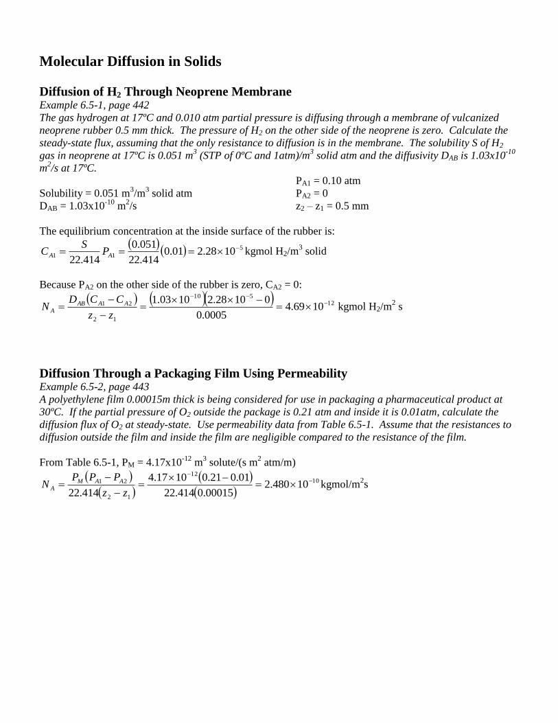
Diffusion of H2 Through Neoprene Membrane Example 6.5-1, page 442

The gas hydrogen at 17ºC and 0.010 atm partial pressure is diffusing through a membrane of vulcanized

neoprene rubber 0.5 mm thick. The pressure of H2 on the other side of the neoprene is zero. Calculate the

steady-state flux, assuming that the only resistance to diffusion is in the membrane. The solubility S of H2

gas in neoprene at 17ºC is 0.051 m3 (STP of 0ºC and 1atm)/m

3 solid atm and the diffusivity DAB is 1.03x10

-10

m2/s at 17ºC.

Solubility = 0.051 m3/m

3 solid atm

DAB = 1.03x10-10

m2/s

PA1 = 0.10 atm

PA2 = 0

z2 – z1 = 0.5 mm

The equilibrium concentration at the inside surface of the rubber is:

5

11 1028.201.0414.22

051.0

414.22

AA PS

C kgmol H2/m3 solid

Because PA2 on the other side of the rubber is zero, CA2 = 0:

12510

12

21 1069.40005.0

01028.21003.1

zz

CCDN AAAB

A kgmol H2/m2 s

Diffusion Through a Packaging Film Using Permeability Example 6.5-2, page 443

A polyethylene film 0.00015m thick is being considered for use in packaging a pharmaceutical product at

30ºC. If the partial pressure of O2 outside the package is 0.21 atm and inside it is 0.01atm, calculate the

diffusion flux of O2 at steady-state. Use permeability data from Table 6.5-1. Assume that the resistances to

diffusion outside the film and inside the film are negligible compared to the resistance of the film.

From Table 6.5-1, PM = 4.17x10-12

m3 solute/(s m

2 atm/m)

1012

12

21 10480.200015.0414.22

01.021.01017.4

414.22

zz

PPPN AAM

A kgmol/m2s

2.0 atm

N2

0 atm

6.5-5 Diffusion Through a Membrane in Series Nitrogen gas at 2.0 atm and 30ºC is diffusing through a membrane of nylon 1.0 mm thick and polyethylene

8.0 mm thick in series. The partial pressure at the other side of the two films is 0 atm. Assuming no other

resistances, calculate the flux, NA at steady state.

P1 = 2.0 atm

P2 = 0 atm

PN2/Ny = 0.152 x 10-12

m2/s atm

PN2/Poly = 1.52 x 10-12

m2/s atm

Diffusion of gas through a solid:

CA can be related to the permeability: 414.22

AA

PSC

where S is the solubility

The permeability of a gas in a solid, PM = DABS

When there are several solids with thicknesses L1, L2,…, we can write the flux as:

12

1212

2

2

1

1

21 10256.1

1052.1

008.0

100152.0

001.0

1

414.22

00.21

414.22

MM

AAA

P

L

P

L

PPN kmole/m

2s

12

21

zz

CCDN AAAB

A

Diffusion in Porous Solids That Depends on Structure

Diffusion of KCl in Porous Silica Example 6.5-3, page 445

A sintered solid of silica 2.0mm thick is porous, with a void fraction ε of 0.30 and tortuosity τ of 4.0. The

pores are filled with water at 298K. At one face the concentration of KCl is held at 0.1 gmol/liter, and fresh

water flows rapidly past the other face. Neglecting any other resistance but that in the porous solid,

calculate the diffusion of KCl at steady-state.

DAB = 1.87x10-9

m2/s from Table 6.3-1 (page 431)

CA1 = 0.1 gmol/liter = 0.1 kgmol/m3

CA2 = 0

τ = 4.0

ε = 0.30

z2 – z1 = 0.002 m

99

12

21 1001.7002.0

01.01087.1

0.4

30.0

zz

CCDN AAAB

A

kgmol/m

2s

P1 = 2.026 x 105 Pa

P2 = 0 Pa

1.25m

6.5-6 Diffusion of CO2 in a Packed Bed of Sand It is desired to calculate the rate of diffusion of CO2 gas in air at steady state through a loosely packed bed

of sand at 276K and a total pressure of 1.013 x 105 Pa. The bed depth is 1.25m and the void fraction ε is

0.30. The partial pressure of CO2 is 2.026 x 103 Pa at the top of the bed and 0 Pa at the bottom. Use a τ of

1.87. τ = 1.87 PA1 = 2.026 x 10

3 Pa

ε = 0.30 PA2 = 0 Pa

T = 276K

025.187.1276314.8

010026.230.010142. 34

12

21

zzRT

PPDN AAAB

A

610609.1 AN mol/m

2s

Unsteady-State Diffusion in Various Geometries

Unsteady-State Diffusion in a Slab or Agar Gel Example 7.1-1, page 463

A solid slab of 5.15 wt% agar gel at 278K is 10.16 mm thick and contains a uniform concentration of urea of

0.1 kgmol/m3. Diffusion is only in the x-direction through two parallel flat surfaces 10.16 mm apart. The

slab is suddenly immersed in pure turbulent water, so the surface resistance can be assumed to be

negligible; that is, the convective coefficient kc is very large. The diffusivity of urea in agar from Table 6.4-2

is 4.72x10-10

m2/s.

(a) Calculate the concentration at the midpoint of the slab (5.08mm from the surface) and 2.54mm from the

surface after 10 hours.

(b) If the thickness of the slab is halved, what would the midpoint concentration be in 10 hours?

C0 = 0.10 kgmol/m3

C1 = 0 for pure water

C = concentration at distance x from the center

line and at time t

DAB = 4.72x10-10

m2/s

t = 10 hours * 3600 seconds = 36000 seconds

1.01.00.1/0

0.1/0

/

/

01

1 cc

CKC

CKCY

(a)

X1 = 10.16mm/2 = 5.08mm = 0.00508 m

X = 0 (center)

658.000508.0

360001072.42

10

2

1

X

tDX AB

Relative position, n = X/X1 = 0

Relative Resistance, m = 0

On Figure 5.3-5 “Unsteady State Conduction in a Large Flat Plate” when X = 0.685, m = 0, n = 0

1.0275.0

cY c = 0.0275 kgmol/m

3

On Figure 5.3-5, when X = 0.658, m = 0, n = 0.00254/0.00508 = 0.5: (n is not 0 now because not at center)

1.0172.0

cY c = 0.0172 kgmol/m

3

(b)

If the thickness is halved, X becomes:

632.200254.0

360001072.42

10

2

1

X

tDX AB

Relative position, n = 0, m = 0

1.00020.0

cY c = 0.0002 kgmol/m

3

7.1-5 Unsteady State Diffusion in a Cylinder of Agar Gel – Radially and Axially A wet cylinder of agar gel at 278K containing a uniform concentration of urea of 0.1 kgmol/m

3 has a

diameter of 30.48mm and is 38.1mm long with flat parallel ends. The diffusivity is 4.72 x 10-10

m2/s.

Calculate the concentration at the midpoint of the cylinder after 100h for the following cases if the cylinder

is suddenly immersed in turbulent pure water.

(a) For radial diffusion only

(b) Diffusion occurs radially and axially

Assume surface resistance is negligible; assume k = 1.0 because properties are similar

T = 278 K

C0 = 0.1 kgmol/m3

C1 = 0 for pure water

D = 4.72 x 10-10

m/s

Time, t = 100h = 360000 seconds

1.01.00.10

0.10

01

1 cc

ckc

ckcY

(a)

r1 = 0.01524 m

r0 = 0 m (center line)

731601.0

01524.0

3600001072.4 10

2

1

r

tDX AB

Relative position at midpoint of the cylinder, n = 0/0.1524 = 0

Relative resistance, m ≈ 0 because kc is assumed to be very large

From Figure 5.3-7, “Unsteady-State Heat Conduction in a Long Cylinder”:

Using X = 0.731601, m = 0, n = 0 Y = 0.024 = c/0.1

Concentration = 0.0024 kgmol/m3

(b)

X1 = L/2 = 38.1 mm / 2 = 19.05 mm = .01905 m

468.0

01905.0

3600001072.4 10

2

1

r

tDX AB

From Figure 5.3-7, Unsteady-State Heat Conduction in a Long Cylinder:

Using X = 0.468, m = 0, n = 0 Y = 0.375

For both axial and radial diffusion, Y = YxYy = (0.375)(0.24) = 0.009

Concentration = 0.0009 kgmol/m3

Unsteady-State Diffusion in a Semi-Infinite Slab Example 7.1-2, page 465

A very thick slab has a uniform concentration of solute A of C0 = 1.0x10-2

kgmol A/m3. Suddenly, the front

face of the slab is exposed to a flowing fluid having a concentration C1 = 0.10 kgmol A/m3 and a convective

coefficient kc = 2x10-7

m/s. The equilibrium distribution coefficient K = cLi/ci = 2.0. Assuming that the slab

is a semi-infinite solid, calculate the concentration in the solid at the surface (x = 0) and x = 0.01m from the

surface after t = 30000 seconds. The diffusivity in the solid is DAB = 4x10-9

m2/s.

t = 3000 seconds

DAB = 4x10-9

m2/s

C0 = 0.01 kgmol.m3

C1 = 0.10 kgmol/m3

kc = 2x10-7

m/s

K = 2.0

095.13000104104

1020.2 9

9

7

tDD

KkAB

AB

c

For x = 0.01:

457.0

30001042

01.0

2 9-

tD

x

AB

From the chart 5.3-3 “Unsteady State Heat Conducted in a Semi-Infinite Solid with Surface Convection”:

26.001.02/1.0

01.0

/1

01

0

C

CKC

CCY C = 2.04x10

-2 kgmol/m

3

For x = 0

0

30001042

0

2 9-

tD

x

AB

From the chart 5.3-3 “Unsteady State Heat Conducted in a Semi-Infinite Solid with Surface Convection”:

62.001.02/1.0

01.0

/1

01

0

C

CKC

CCY C = 3.48x10

-2 kgmol/m

3

This is the same value as Ci. To calculate CLi:

22 1096.61048.30.2 iLi KCC kgmol/m3

7.1-6 Drying of Wood – Unsteady State Diffusion in a Flat Plate A flat slab of Douglas fir wood 50.8mm thick containing 30 wt% moisture is being dried from both sides

(neglecting ends and edges). The equilibrium moisture content at the surface of the wood due to the drying

air blown over it is held at 5 wt% moisture. The drying can be assumed to be represented by a diffusivity of

3.72 x 10-6

m2/h. Calculate the time for the center to reach 10% moisture.

Assume there is no surface resistance and kc = ∞

At t = 0, c0 = 0.3, c1 = 0.05

At t = ?, c = 0.1

DAB = 3.72 x 10-6

m2/h

Solve for Y: 2.03.00.15.0

1.00.15.0

01

1

ckc

ckcY

Solve for X for the graph:

X1 = 25.4 mm = 0.254 m

X0 (center) = 0 m

tt

x

tDX AB 005766.0

254.0

1072.32

6

2

1

Relative position, n = 0 at the center

Relative resistance, m = 0 because kC is large

From Chart 5.3-5, “Unsteady State Heat Conduction in a Flat Plate”: X = 0.75 = 0.005766t

Time, t = 130.073 hours

Convective Mass Transfer Coefficients Vaporizing A and Convective Mass Transfer Example 7.2-1, page 469

A large volume of pure gas B at 2 atm pressure is flowing over a surface from which pure A is vaporizing.

The liquid A completely wets the surface, which is a blotting paper. Hence, the partial pressure of A at the

surface is the vapor pressure of A at 298K, which is 0.2 atm. The k’y has been estimated to be 6.78x10

-5

kgmol/s m2 mol frac. Calculate NA, the vaporization rate, and also the value of ky and kG.

P = 2.0 atm

PA1 = 0.2 atm

PA2 = 0 atm

k'y = 6.78x10

-5 kgmol/s m

2 mol frac

First calculate the mole fraction of A:

1.00.2/2.0/1 PPY AA

02 AY

To calculate ky, we must relate it to k'y:

'

yBMy kyk

95.0

9.0/0.1ln

9.01

ln 12

12

BB

BBBM

yy

yyy

55'

10138.795.0

1078.6

BM

y

yy

kk kgmol/m

2 s mole fraction

Now we can calculate kG:

BMyBMG ykPyk 55

10569.30.2

10138.7

P

kk

y

G kgmol/m2 s atm

Now we can calculate the vaporization rate, NA:

65

21 10138.7010.010138.7 AAyA yykN kgmol/m2s

or

65

21 10138.702.010569.3 AAGA PPkN kgmol/m2s

7.2-1 Flux and Conversion of Mass-Transfer Coefficient A value of kG

was experimentally determined to be 1.08 lbmol/h ft

2 atm for A diffusing through stagnant B.

For the same flow and concentrations it is desired to predict kG’ and the flux of A for equimolar

counterdiffusion. The partial pressures are PA1 = 0.20 atm, PA2 = 0.05 atm, P = 1.0 atm abs total. Use

English and SI Units.

BMGG PkPk '

Solve for PBM:

872853.0

2.01

05.01ln

05.02.0

ln1

2

21

A

A

AABM

PP

PP

PPP atm

Plug into equation:

k’G (1.0 atm) = (1.08 lbmol/h ft

2 atm)(0.872853 atm)

k’G(1.01x10

5Pa) = (1.08lbmol/hft

2atm)(.872853atm)(1hr/3600sec)(1ft

2/.0929 m

2)(.453kgmol/lbmol)

k’G = 0.9427 lbmol/h ft

2 atm

k’G = 1.262 x 10

-8 kgmol/s m

2 Pa

Now solve for flux:

PA1 = 0.2 atm = 20265 Pa

PA2 = 0.05 atm = 5066.25 Pa

1414.05.02.09247.021

' AAGA PPkN

48

21

' 1092.125.50662026510262.1 AAGA PPkN

NA = 0.1414 lbmol/ft2h

NA = 1.92 x 10-4

kgmol/m2s

Mass Transfer Under High Flux Conditions

High Flux Correction Factors Example 7.2-2, page 472

Toluene A is evaporating from a wetted porous slab by having inert pure air at 1 atm flowing parallel to the

flat surface. At a certain point, the mass transfer coefficient, k’x for very low fluxes has been estimated as

0.20 lbmol/hr ft2. The gas composition at the interface at this point is XA1 = 0.65. Calculate the flux NA and

the ratios kc/ k’c or kx/ k

’x and k

0c/ k

’c or k

0x/ k

’x to correct for high flux.

First find XBM:

619.0

65.01

01ln

65.0101

ln1

2

12

B

B

BBBM

X

X

XXX

To find the flux, NA, use:

210.0065.0619.0

20.021

'

AA

BM

x

A XXX

kN lbmol/ft

2 hr

To find the ratios, set up the following:

616.1619.0

11''

BMc

c

x

x

Xk

k

k

k

So 323.02.0616.1616.1 ' xx kk lbmol/ft2 hr; and

565.0619.0

65.011 1

'

0

'

0

BM

A

c

c

x

x

X

X

k

k

k

k

So 113.02.0565.0565.0 '0 xx kk lbmol/ft2 hr

1 2

7.2-3 Absorption of H2S by Water In a wetted-wall tower an air H2S mixture is flowing by a film of water that is flowing as a thin film down a

vertical plate. The H2S is being absorbed from the air to the water at a total pressure of 1.50 atm abs and

30ºC. A value for kc’ of 9.567 x 10-4

m/s has been predicted for the gas-phase mass transfer coefficient. At a

given point, the mole fraction of H2S in the liquid at the liquid-gas interface is 2.0(10-5

) and PA of H2S in the

gas is 0.05 atm. The Henry’s law equilibrium relation is PA (atm) = 609xA (mole fraction in the liquid).

Calculate the rate of absorption of H2S. Hint: Call point 1 the interface and point 2 the gas phase. Then

calculate PA1 from Henry’s Law and the given xA. The value of PA2 is 0.05 atm.

P = 1.50 atm

PA1 = 609 (CA1) = 609(2 x 10-5

) = 0.01218 atm

PA2 = 0.05 atm

T = 30 ºC = 303.15 K

k’c = 9.567 x 10

-4 m/s

XA1 = 2 x 10-5

Henry’s Law: PA = 609XA

R = 82.057 x 10-3

m3 atm/kgmol K

PkRT

PkG

c ''

5

3

4' 10846.3

15.30310057.82

10567.9

Gk kgmol/m

2s atm

65

21 10455.105.001218.010846.3 AAGA PPkN

NA = 1.455 x 10-6

kgmol/m2s

Mass Transfer for Flow Inside Pipes

Mass Transfer Inside a Tube Example 7.3-1, page 479

A tube is coated on the inside with naphthalene and has an inside diameter of 20 mm and a length of 1.10m.

Air at 318K and an average pressure of 101.3 kPa flows through this pipe at a velocity of 0.80 m/s.

Assuming that the absolute pressure remains essentially constant, calculate the concentration of naphthalene

in the exit air.

v = 0.80 m/s

D = 0.02 m

T = 318 K

z2 – z1 = 1.10 m

DAB = 6.92x10-6

m2/s

PAi = 74.0 Pa

μair = 1.932x10-5

Pa s from Appendix A

ρ = 1.114 kg/m3

R = 8314 m3 Pa/kgmol K

Calculate the concentration, CAi:

510799.23188314

74 RT

PC Ai

Ai kgmol/m3

Calculate the Schmidt number:

506.2

1092.6114.1

10932.16

5

AB

ScD

N

Calculate the Reynolds number:

6.922

10932.1

114.180.002.05Re

DN

Hence, the flow is laminar. We will use Figure 7.3-2 for laminar flow streamlines:

02.33410.1

02.0506.26.922

4Re

L

DNN Sc

Using Figure 7.3-2 with rodlike flow:

55.00

0

AAi

AA

CC

CC

If CA0 = 0,

010799.2

055.0

5

0

0

A

AAi

AA C

CC

CC CA = 1.539 x 10

-5 kgmol/m

3

Pure Water

T = 26.1ºC

v = 3.05m/s

0.00635 m

1.22 m

1.829 m

7.3-7 Mass Transfer from a Pipe and Log Mean Driving Force Use the same physical conditions as in problem 7.3-2, but the velocity in the pipe is now 3.05

m/s. Do as follows:

(a) Predict the mass transfer coefficient kc (Is this turbulent flow?).

(b) Calculate the average benzoic acid concentration at the outlet. [ Note: in this case,

Eqs. (7.3-42) and (7.3-43) must be used with the log mean driving force, where A is

the surface area of the pipe.]

(c) Calculate the total kgmol of benzoic acid dissolved per second.

ρ = 996 kg/m3

μ = 8.71 x 10-4

Pa s

T = 26.1ºC

DAB = 1.245x10-9

m2/s

Solubility = 0.2948 kgmol/m3

D = 0.00635 m

As = 2rπL

V = Aυ

Calculate the Schmidt number:

408.702

10245.1996

1071.89

4

AB

ScD

N

Calculate the Reynolds number:

22147

1071.8

99605.300635.04Re

DN

Calculate the Sherwood number:

000049487.023.033.083.0

Re ScSh NNN

Now calculate k’c:

AB

c

ShD

DkN

'

00635.0

10245.1000049487.0

9' ck

4' 1059.1 ck m/s

(b)

CA1 = 0

CAi = 0.02948 (solubility)

CA2 = ?

So now we plug this into the log mean driving force equation:

2

1

1212

lnAAi

AAi

AACAA

CC

CC

CCKACCv

CA1 = 0, so it cancels out of the equation:

2

22

lnAAi

Ai

ACA

CC

C

CKACv

Now plug in:

2

242

2

02948.0

02948.0ln

1059.1003175.005.3

A

AA

C

CC

CA2 = 0.001151 kgmol/m3

(c)

Rate of benzoic acid dissolved = NA:

7

2

12 1011.1003175.0

0001151.005.3

A

CCvN AA

A

Mass Transfer for Flow Outside Solid Surfaces Mass Transfer From a Flat Plate

Example 7.3-2, page 481

A large volume of pure water at 26.1ºC is flowing parallel to a flat plate of solid benzoic acid, where L =

0.24 m in the direction of flow. The water velocity is 0.061 m/s. The solubility of benzoic acid in water is

0.02948 kgmol/m3. The diffusivity of benzoic acid is 1.245x10

-9 m

2/s. Calculate the mass-transfer coefficient

kL and the flux NA.

Solubility = 0.02948 kgmol/m3

T = 26.1ºC

L = 0.24 m

DAB = 1.245x10-9

m2/s

v = 0.061 m/s

Because the solution is dilute, we can use the properties of water for the solution:

ρ = 996 kg/m3

μ = 8.71 x 10-4

Pa s

Calculate the Schmidt Number:

702

10245.1996

1071.89

4

AB

ScD

N

Calculate the Reynolds number:

17000

1071.8

996061.024.04Re

DN

Now calculate JD:

00758.01700099.099.05.05.0

Re,

LD NJ

Now solve for k’c:

3/2'

Sc

c

D Nk

J

6' 1085.5 ck m/s

In this case, A is diffusing through stagnant B. We use the solubility for CA1 and CA2 = 0. Also, since the

solution is dilute, xBM ≈ 1:

76

21

'

10726.1002948.00.1

1085.5

AA

BM

c

A CCX

kN kgmol/m

2s

Mass Transfer From a Sphere Example 7.3-3, page 482

Calculate the value of the mass-transfer coefficient and the flux for mass transfer from a sphere of

naphthalene to air at 45ºC and 1 atm abs flowing at a velocity of 0.305 m/s. The diameter of the sphere is

0.0254m. The diffusivity of naphthalene in air at 45ºC is 6.92x10-6

m2/s and the vapor pressure of solid

naphthalene is 0.555 mmHg.

D = 0.0254m

PA1 = 0.555 mmHg = 74 Pa

T = 45ºC

P = 1 atm

v = 0.305 m/s

DAB = 6.92x10-6

m/s

ρ = 1.113 kg/m3

μ = 1.93 x 10-5

Pa s

Calculate the Schmidt number:

505.2

1092.6113.1

1093.16

5

AB

ScD

N

Calculate the Reynolds number:

446

1093.1

113.1305.00254.05Re

DN

Now find the Sherwood number:

0.21552.023/153.0

Re ScSh NNN

Now solve for k’c:

AB

cshD

DkN ' 3

6' 1072.5

0254.0

1092.60.21

D

DNk AB

shc m/s

Now solve for k’G:

9

3'

' 10163.23188314

1072.5

RT

kk c

G kgmol/s m2 Pa

Since the gas is dilute, k’G ≈ kG. Using that we can solve for the flux:

79

21 10599.107310163.2 AAGA PPkN kgmol/m2 s

7.3-1 Mass Transfer from a Flat Plate to a Liquid Using the data and physical properties from Example 7.3-2, calculate the flux for a water velocity of 0.152

m/s and a plate length of L = 0.137 m. Do not assume that xBM = 1.0 but actually calculate its value.

DAB = 1.245 x 10

-9 m

2/s

Solubility, S = 0.02948 kgmol/m3

ρ = 996 kg/m3

Mw = 18 kg/kgmol

CA1 = 0.02948 kgmol/m3

μ = 8.71 x 10-9

Pa s

Solve for XBM:

XB1 = 11

1

AB

B

CC

C

= [(996 kg/m

3)/(18kg/kgmol)]/[(996 kg/m

3)/(18kg/kgmol) + 0.02948 kgmol/m

3]

XB1 = 0.999468

XB2 = 1.0

999734.0

999468.0

0.1ln

999468.00.1

ln1

1ln

1

2

12

1

2

21

B

B

BB

A

A

AABM

X

X

XX

X

X

XXX

Calculate Schmidt Number:

70210245.1996

1071.89

4

AB

SCD

N

Calculate Reynolds Number:

5.23812

1071.8

996152.0137.09Re

LN

Calculate JD:

06416.05.2381299.099.05.05.0

Re

NJ D

Calculate K’c:

53/23/2' 102346.1702152.006416.0 SCDC NJK m/s

Calculate Flux:

75

21

'

10641.3999734.0

02948.0102346.1

BM

AAC

AX

CCKN kgmol/m

2s

7.3-4 Mass Transfer to Definite Shapes – Flat Plate and a Sphere Estimate the value of the mass-transfer coefficient in a stream of air at 325.6 K flowing in a duct past the

following shapes made of solid naphthalene. The velocity of the air is 1.524 m/s at 325.6K and 202.6 kPa.

The DAB of naphthalene in air is 5.16 x 10-6

m2/s at 273K and 101.3 kPa.

(a) For air flowing parallel to a flat plate 0.152 m in length

(b) For air flowing past a single sphere 12.7 mm in diameter

CA1

0.137 m

Benzoic Acid

Water at 26.1ºC, velocity, v = 0.152 m/s

P = 202600 Pa

R = 8314.34 m3 Pa/kgmol K

T = 325.6 K

Mw = 28.8 kg/kgmol

Correct DAB:

6

175.1175.1

1051182.33.101

6.202

273

6.3256.202,6.325

ooABP

P

T

TkPaKD m

2/s

Calculate ρ and μ:

1958.0273

6.3250171.0

768.0

cP

T

Tn

o

o cP = 1.958 x 10-5

kg/m s

155.26.32534.8314

2026008.28

RT

PM w kg/m3

(a)

Calculate NRe:

5.25495

10958.1

155.2524.1152.05Re

LN

Because NRe > 15000:

004732.05.25495036.0036.02.02.0

Re NJ D

58722.2

1051182.3155.2

10958.16

5

AB

SCD

N

3/2'

SC

C

D NK

J

3/2'

58722.2524.1

004732.0 CK K

’C = 0.003827 m/s

9

'

1041366.16.32534.8314

003827.0 RT

KK C

G kgmol/m2 Pa s

(b) Dp = 0.0127 m

Calculate Reynolds and Schmidt Numbers:

21.2130

10958.1

155.2524.10127.05Re

pDN

58722.2

1051182.3155.2

10958.16

5

AB

SCD

N

Because 0.6 < NSC < 2.7:

0164.4658722.221.2130552.02552.023/153.03/153.0

Re SCSH NNN

Air at 325.6K, 202.6 kPa, v = 1.524 m/s

0.152 m

AB

pC

SHD

DKN

'

6

'

1051182.3

0127.00164.46

CK

K’C = 0.012725 m/s

9

'

1070.46.32534.8314

012735.0 RT

KK C

G kgmol/m2 Pa s

Mass Transfer of a Liquid in a Packed Bed Example 7.3-4, page 485

Pure water at 26.1ºC flows at the rate of 5.514x10-7

m3/s through a packed bed of benzoic acid spheres

having diameters of 6.375mm. The total surface area of the spheres in the bed is 0.01198 m2 and the void

fraction is 0.436. The tower diameter is 0.0667m. The solubility of benzoic acid in water is 2.948x10-2

kgmol/m3.

(a) Predict the mass transfer coefficient kc.

(b) Using the experimental value of kc, predict the outlet concentration of benzoic acid in the water.

Because the solution is dilute, we can use the properties of water for the solution:

ρ = 996 kg/m3

μ26.1ºC = 8.71 x 10-4

Pa s

μ25ºC = 8.94 x 10-4

Pa s

V = 5.514x10-7

m3/s

Dp = 6.375mm

AS = 0.01198 m2

ε = 0.436

D = 0.0667m

S = 2.948x10-2

kgmol/m3

DAB(25ºC) = 1.21x10-9

m2/s from Table 6.3-1

Correct DAB:

9

3

39 10254.1

108718.0

108940.0

298

1.2991021.1251.26

new

old

old

new

ABABT

TDD

m

2/s

Calculate the area of the column:

32 10494.30667.044

DA m2

Now use the area and volumetric flow to find the velocity:

437 10578.110494.3/10514.5/ AVv m/s

Calculate the Schmidt Number:

6.702

10245.17.996

1071.89

4

AB

ScD

N

Calculate Reynolds number:

150.1

1071.8

7.99610578.1006375.04

4

Re

pDN

Calculate JD:

277.2150.1436.

09.109.1 3/23/2

Re

NJ D

Then, assuming k’c = kc for dilute solutions,

3/2'

Sc

c

D Nv

kJ 3/2

4

'

6.70210578.1

277.2

ck 6' 10447.4 ck m/s

Now set the log mean driving force equation can be set equal to the material balance equation on

the bulk stream:

12

2

1

21

ln

AA

AAi

AAi

AAiAAi

c CCV

CC

CC

CCCCAk

where CAi = 0.02948 (the solubility)

CA1 = 0

A = 0.01198 m2 (the surface area of the bed)

V = 5.514x10-7

m3/s

CA2 = 2.842 x 10-3

kgmol/m3

7.3-5 Mass Transfer to Packed Bed and Driving Force Pure water at 26.1ºC is flowing at a rate of 0.0701ft

3/h through a packed bed of 0.251-in.

benzoic acid spheres having a total surface area of 0.129 ft2. The solubility of benzoic acid in

water is 0.00184 lbmol benzoic acid/ft3 solution. The outlet concentration is cA2 is 1.80 x 10

-4

lbmol/ft3. Calculate the mass transfer coefficient kc. Assume dilute solution.

μ = 0.8718 x 10-3

Pa s

ρ = 996.7 kg/m3

υ = 0.0701 ft3/hr

A = 0.129

CAi = 0.00184 lbmol/ft3

CA1 ≈ 0

CA2 = 1.80 x 10-4

lbmol/ft3

Log mean driving force equation:

2

1

12

lnAAi

AAi

AACA

CC

CC

CCKAAN

where CA1 is the inlet bulk flow concentration, CA2 is the outlet bulk flow concentration, and CAi is the

concentration at the surface of the solid (which in this case equals the solubility)

Material Balance on the bulk stream: 12 AAA CCvAN

So now we plug this into the log mean driving force equation:

2

1

1212

lnAAi

AAi

AACAA

CC

CC

CCKACCv

CA1 = 0, so it cancels out of the equation:

2

22

lnAAi

Ai

ACA

CC

C

CKACv

We can now plug in given numbers:

4

44

1080.100184.0

00184.0ln

1080.1129.01080.10701.0 CK KC = 0.0559 ft/hr

Mass Transfer to Suspensions of Small Particles Mass Transfer from Air Bubbles in Fermentation Example 7.4-1, page 488

Calculate the maximum rate of absorption of O2 in a fermenter from air bubbles at 1 atm abs pressure

having diameters of 100 μm at 37ºC into water having a zero concentration of dissolved oxygen. The

solubility of O2 from air in water at 37ºC is 2.26x10-7

kgmol O2/m3 liquid. The diffusivity of O2 in water at

37ºC is 3.25x10-9

m2/s. Agitation is used to produce the air bubbles.

Dp = 1 x 10-4

m

DAB = 3.25x10-9

m2/s

Solubility = 2.26x10-7

kgmol O2/m3 liquid

μc,water = 6.947 x 10-4

Pa s = 6.947 x 10-4

kg/ m s

ρc,water = 994 kg/m3

ρp,air = 1.13 kg/m3

Calculate NSc:

215

1025.3994

10947.69

4

ABc

c

ScD

N

Now calculate k’L:

3/1

2

3/2' 31.02

c

c

Sc

p

ABL

gN

D

Dk

4

3/1

2

43/2

4

9' 1029.2

994

806.910947.613.199421531.0

101

1025.32

Lk m/s

Assuming k’L = kL for dilute solutions,

874

21 1018.501026.21029.2 AALA CCkN kgmol O2/m2 s

Molecular Diffusion Plus Convection and Chemical Reaction Proof of Mass Flux Equation Example 7.5-1, page 491

Table 7.5-1 gives the following relation: 0 BA jj

Prove this relationship using the definition of the fluxes in terms of velocities.

From Table 7.5-1 (page 490), substituting AA for jA and BB for jB, and rearranging:

0 BBBAAA 0 BABBAA

BB

AA

and BA

0

B

BA

ABBAA 0 BBAABBAA

Thus the identity is proved.

Diffusion and Chemical Reaction at a Boundary Example 7.5-2, page 495

Pure gas A diffuses from point 1 at a partial pressure 101.32 kPa to point a distance 2.00mm away. At point

2, it undergoes a chemical reaction at the catalyst surface and A 2B. Component B diffuses back at

steady state. The total pressure is P = 101.32 kPa. The temperature is 300K and DAB = 0.15 x 10-4

m2/s.

(a) For instantaneous rate of reaction, calculate xA2 and NA.

(b) For a slow reaction where k’1 = 5.63x10

-3 m/s, calculate xA2 and NA.

PA2 = XA2 = 0 because no A can exist next to the

catalyst surface

XA1 = PA1/P = 1.0

δ = 0.002 m

T = 300 K

C = P/RT = 101320/(8314*300) = 4.062 x 10-2

kgmol/m3

NB = -2NA

DAB = 0.15 x 10-4

m2/s

k’1 = 5.63x10

-3 m/s

(a)

442

2

1 10112.201

0.11ln

002.0

1015.010062.4

1

1ln

A

AABA

X

XCDN

kgmol A/m

2s

(b)

SubstituteCk

NX A

A '

1

2 in for XA2:

Ck

N

XCDN

A

AABA

'

1

1

1

1ln

4

23

42

10004.1

10062.41063.51

0.11ln

002.0

1015.010062.4

A

A NN kgmol A/m

2s

7.5-7 Unsteady State Diffusion and Reaction Solute A is diffusing at unsteady state into a semi-infinite medium of pure B and undergoes a first-order

reaction with B. Solute A is dilute. Calculate the concentration CA at points z = 0, 4, and 10 mm from the

surface for t = 1 x 105 seconds. Physical property data are DAB = 1 x 10

-9 m

2/s, k’ = 1 x 10

-4 s

-1, CA0 = 1.0 kg

mol/m3. Also calculate the kg mol absorbed/m

2. Find CA and Q.

For un-steady state diffusion and homogenous reaction in a semi-infinite medium,, the general solution is:

tk

tD

zerf

D

kztk

tD

zerf

D

kz

C

Ci

ABAB

i

ABAB

A

2exp

2exp

'

12

1

'

12

1

For z1=0m:

542

1542

1 1011010exp1011010exp0.1

erferfCA

0.100exp20exp 21

21 AC kgmol/m

3

For z2=0.004m

54

959

4

21

54

959

4

21

1011011011012

004.0

101

101004.0exp

1011011011012

004.0

101

101004.0exp

0.1

erf

erfCA

28226.02282264.00101

101004.0exp2

101

101004.0exp 2

19

4

21

9

4

21

AC kgmol/m3

For z2=0.01m

54

959

4

21

54

959

4

21

1011011011012

01.0

101

10101.0exp

1011011011012

01.0

101

10101.0exp

0.1

erf

erfCA

9998.1042329.00101

10101.0exp9998.1

101

10101.0exp 2

19

4

21

9

4

21

AC

0423.0.0AC kgmol/m3

(b)

The total amount, Q, of A absorbed up to time t is represented by:

tkAB

A etk

tkerftkk

DcQ

''

'

21'

'0

Plugging in and solving for Q, we get:

54 101101

5454

2154

'4

9 101101101101101101

101

1011 eerfQ

0332.0Q kgmol/m2

7.5-11 Effect of Slow Reaction Rate on Diffusion Gas A diffuses from point 1 to a catalyst surface at point 2, where it reacts as follows: 2A B. Gas B

diffuses back a distance δ to point 1.

(c) Derive an equation for NA for a slow first-order reaction where k1’ is the reaction velocity constant.

(d) Calculate NA and xA2 for part (c) where k1’ – 0.53 x 10-2

m/s.

(c)

Begin with the convective diffusion equation:

BAAA

ABA NNC

C

dz

dCDN where: AB

AA NN

C

Cx

21,

Plugging in:

21

21ln

2

21

1

2

0

21

2

1

A

AABA

x

x A

ABAAAA

ABA

x

xCDN

x

dxCDdzNNx

dz

dxCDN

A

A

For a slow reaction, Ck

Nx A

A '

1

2 . Plugging into the flux equation and replacing C with P/RT:

21

21ln

2

1

'

1

A

AABA

x

PkRTN

RT

PDN

(d)

Plugging in the values, we get:

297.01

1001325.11053.02298314.81ln

0013.0298314.8

102.01001325.125245

AA

NN

41076.1 AN kgmol/m2 s

Solving for the mole fraction:

81479.0

298314.8

1001325.10053.0

1076.15

4

'

1

2

Ck

Nx A

A

7.5-10 Diffusion and Chemical Reaction of Molten Iron in Process Metallurgy In a steel-making process using molten pig iron containing carbon, a spray of molten iron particles

containing 4.0 wt % carbon falls through a pure oxygen atmosphere. The carbon diffuses through the

molten iron to the surface of the drop, where it is assume that it reacts instantly at the surface because of the

high temperature, as follows, according to a first order reaction:

Calculate the maximum drop size allowable so that the final drop after a 2.0 second fall contains an average

of 0.1 wt % carbon. Assume that the mass transfer rate of gases at the surface is very great, so there is no

outside resistance. Assume no internal circulation of the liquid. Hence, the decarburization rate is

controlled by the rate of diffusion of carbon to the surface of the droplet. The diffusivity of the carbon in

iron is 7.5 x 10-9

m2/s (S7). Hint: use figure 5.3-13

For unsteady-state diffusion through a spherical geometry where we are looking at average temperature and

time, Figure 5.3-13 (page 377) can be used. So, to find the radius, r, we need to find Y, and X, where:

025.00040

001.00

01

1

CC

CCY ave

Because A reacts instantly, we know that C1=0. From the graph for a sphere at Y, X=0.32

Solving for r:

2

1

9

2

1

2105.732.0

rr

tDX AB

000217.0r m

Unsteady State Diffusion and Reaction in a Semi-Infinite Medium Reaction and Unsteady State Diffusion Example 7.5-3, page 498

Pure CO2 gas at 101.32 kPa pressure is absorbed into a dilute alkaline buffer solution containing a catalyst.

The dilute, absorbed solute CO2 undergoes a first-order reaction, with k’= 35 s

-1 and DAB = 1.5x10

-9 m

2/s.

The solubility of CO2 is 2.961x10-7

kgmol/m3 Pa. The surface is exposed to the gas for 0.010 seconds.

Calculate the kgmol CO2 absorbed/m2 surface.

P = 101.32 kPa

k’= 35 s

-1

DAB = 1.5x10-9

m2/s

Solubility of CO2 is 2.961x10-7

kgmol/m3 Pa

Time, t = 0.010 seconds

The total amount, Q, of A absorbed in time, t is:

tk

ABA etktkerftkkDCQ'

// ''

21''

0

k’t = (35s

-1)(0.010s) = 0.350

CA0 = Solubility*Pressure = (2.961x10-7

kgmol/m3 Pa)( 101.32 kPa) = 3.00x10

-2 kgmol CO2/m

3

7350.0

2192 10458.1/350.0350.0350.35/105.11000.3 eerfQ kgmol CO2/m

2

Multicomponent Diffusion of Gases

Diffusion of A Through Nondiffusing B and C Example 7.5-4, page 498

At 298K and 1 atm total pressure, methane (A) is diffusing at steady state through nondiffusing argon (B)

and helium (C). At z1 = 0, the partial pressures in atm are PA1 = 0.4, PB1 = 0.4, PC1 = 0.2, and at z2 =

0.005m, PA2 = 0.1, PB2 = 0.6, PC2 = 0.3. The binary diffusivities from Table 6.2-1 are DAB = 2.02x10-5

m2/s,

DAC = 6.75x10-5

m2/s, and DBC = 7.29x10

-5 m

2/s. Calculate NA.

PA1 = 0.4,

PB1 = 0.4,

PC1 = 0.2

PA2 = 0.1

PB2 = 0.6

PC2 = 0.3

z2 = 0.005m

z1 = 0

T = 298K

P = 1 atm

DAB = 2.02x10-5

m2/s

DAC = 6.75x10-5

m2/s

DBC = 7.29x10-5

m2/s

R = 82.057 m3 atm/kgmol K

Find DAM:

At point 1:

667.04.01

4.0

1

'

A

BB

X

XX

At point 2:

667.01.01

6.0

1

'

A

BB

X

XX

333.0

4.01

2.0

1

'

A

C

CX

XX

5

55

''10635.2

1075.6333.0

1002.2667.0

11

AC

C

AB

B

AM

DX

DX

D m2/s

Calculate PiM:

6.04.00.111 Ai PPP atm

9.01.00.122 Ai PPP atm

740.0

4.09.0ln

4.09.0

ln1

2

12

i

i

ii

iM

PP

PPP atm

Now solve for NA:

55

21

12

1074.86.09.0740.0005.0298057.82

0.110635.2

AA

iM

AMA PP

PzzRT

PDN kgmol A/m

2s

7.5-8 Multicomponent Diffusion At a total pressure of 202.6 kPa and 358 K, ammonia gas (A) is diffusing at steady state through an inert,

nondiffusing mixture of nitrogen (B) and hydrogen (C). The mole fractions at z1 = 0 are xA1 = 0.8, xB1 =

0.15, and xC1 = 0.05; and at z2 = 4.0 mm, xA1 = 0.2, xB1 = 0.6, and xC1 = 0.2. The diffusivities at 358 K and

101.3 kPa are DAB = 3.28 x 10-5

m2/s and DAC = 1.093 x 10

-4 m

2/s. Calculate the flux of ammonia.

For multi-component diffusion, the flux can be calculated as:

21

12

AA

AM

AMA CC

Czz

CDN

Calculate DAM in m2/s:

5

55

1

1

1

1

109878.1

8.0110456.5

05.0

0811064.1

15.0

1

11

1

AAC

C

AAB

B

AM

xD

x

xD

xD

Calculate CAM:

0647.68

3588314

106.202 3

RT

PC mol/m

3

45.548.00647.6811 AA CxC mol/m3

61.132.00647.6822 AA CxC mol/m3

2

1

21

lnA

A

AAAM

CC

CC

CCCCC

4605.29

61.130647.68

45.540647.68ln

61.130647.6845.540647.68

mol/m

3

Substituting back in and solving for flux:

4335

21

12

1068.461.1345.544605.290004.0

0647.68109878.1

molmmolmCC

Czz

CDN AA

AM

AMA

41068.4 AN kgmole/m2s

Knudsen Diffusion of Gases

Knudsen Diffusion of Hydrogen Example 7.6-1, page 500

A H2(A) – C2H6(B) gas mixture is diffusing in a pore of a nickel catalyst used for hydrogenation at

1.01325x105 Pa and 373K. The pore radius is 60

A (angstrom). Calculate the Knudsen diffusivity, DKA, of

H2.

P = 1.01325x105 Pa

T = 373K

r = 60 angstroms = 6.0x10-9

MA(H2) = 2.016

62

1

92

1

1092.7016.2

37310600.970.97

A

KAM

TrD m

2/s

Flux Ratios for Diffusion of Gases In Capillaries

Transition-Region Diffusion of He and N2 A gas mixture at a total pressure of 0.10 atm abs and 298K is composed of N2 (A) and He (B). The mixture

is diffusing through an open capillary 0.010m long having a diameter of 5x10-6

m. The mole fraction of N2

at one end is XA1 = 0.8 and at the other is XA2 = 0.2. The molecular diffusivity DAB is 6.98x10-5

m2/s at 1 atm,

which is an average value based on several investigations.

(a) Calculate the flux NA at steady state.

(b) Use the approximate equations for this case.

L = 0.010m

r = 2.5x10-6

m

P = 0.10 atm

T = 298 K

XA1 = 0.8

XA2 = 0.2

DAB = 6.98x10-5

m2/s

MA = 28.02 kg/kgmol

MB = 4.003 kg/kgmol

R = 8314.3 m3 Pa/kgmol K

(a)

42

1

62

1

1091.702.28

273105.20.970.97

A

KAM

TrD m

2/s

In an open system with no chemical reaction, the ratio of NA/NB is constant:

645.2003.4

02.28

B

A

A

B

M

M

N

N

Now we can solve for the flux factor, α:

645.1645.211 A

B

N

N

Now we can solve for the transition region NA:

KAABA

KAABAABA

DDx

DDx

RTL

PDN

/1

/1ln

1

2

5

45

4545

1040.61091.7/1098.68.0645.11

1091.7/1098.62.0645.11ln

010.02983.8314645.1

10013.11098.6

AN kgmol/m

2s

(b) If we estimate that equimolar counterdiffusion is taking place at steady state, α = 1-1 = 0. We can

estimate the diffusivity, D’NA:

4

45

' 10708.3

1091.71

1098.61

1

11

1

KAAB

NA

DD

D m2/s

Now we can solve for the approximate flux:

5

44

21

'

1010.92.08.0010.02988314

10013.110708.3

AA

NA

A XXRTL

PDN kgmol/m

2s

7.6-4 Transition-Region Diffusion in Capillary A mixture of nitrogen gas (A) and helium (B) at 298 K is diffusing through a capillary 0.10 m long in an

open system with a diameter of 10 μm. The mole fractions are constant at XA1 = 1.0 and XA2 = 0.0. DAB =

6.98 x 10-5

m2/s at 1 atm. MA = 28.02 kg/kg mol, MB = 4.003.

(a) Calculate the Knudsen diffusivity DKA and DKB at the total pressures of 0.001, 0.1 and 10 atm.

(b) Calculate the flux NA at steady state at the pressures.

(c) Plot NA versus P on log-log paper. What are the limiting lines at lower pressures and very high

pressures? Calculate and plot these lines.

(a)

The Knudsen diffusivity for A and B will be the same at all pressures (it is independent of pressure): 2

1

0.97

A

KM

TrD

001582.002.28

2981050.97

21

6

KAD m2/s

004185.0003.4

2981050.97

21

6

KBD m2/s

(b)

For the transition region, flux is calculated using:

KAABA

KAABAABA

DDx

DDx

RTL

PDN

1

2

1

1ln

For P = 0.001:

7

2

22

1021.6001582.01098.616457.11

001582.01098.606457.11ln

1.0298082157.06457.1

001.01098.6

AN kgmol/m

2s

For P = 0.1:

5

2

22

10321.1001582.01098.616457.11

001582.01098.606457.11ln

1.0298082157.06457.1

1.01098.6

AN kgmol/m

2s

For P = 10:

5

2

22

1068.1001582.01098.616457.11

001582.01098.606457.11ln

1.0298082157.06457.1

101098.6

AN kgmol/m

2s

(c)

Lower limit is representative of Knudsen diffusion and the upper limit is representative of molecular

diffusion.

9.3 Vapor Pressure of Water and Humidity

9.3-1 Humidity from Vapor-Pressure Data The air in a room is at 26.7ºC and a pressure of 101.325 kPa and contains water vapor with a partial

pressure pA = 2.76 kPa. Calculate the following:

(a) Humidity, H

(b) Saturation humidity, HS, and percentage humidity, HP.

(c) Percentage relative humidity, HR.

From the steam tables at 26.7ºC, the vapor pressure of water is pAs = 3.50 kPa. Also pA = 2.76 kPa and P =

101.3 kPa. For part (a):

01742.0

76.23.10197.28

76.202.18

97.28

02.18

A

A

pP

pH kg H2O/ky dry air

For part (b)

02226.0

76.23.10197.28

50.302.18

97.28

02.18

As

As

pP

pH

%3.7802226.0

01742.0100100

s

pH

HH

For part (c)

%9.7850.3

76.2100100

As

AR

p

pH

9.3-2 Use of Humidity Chart Air entering a dryer has a temperature (dry bulb) of 60ºC and a dew point of 26.7ºC. Using the humidity

chart, determine the actual humidity H, percentage humidity HP, humid heat cs, and humid volume vH.

The dew point of 26.7ºC is the temperature when the given mixture is at 100% saturation. Starting at 26.7ºC,

and drawing a vertical line until it intersects the line for 100% humidity, a humidity of H = 0.0225 kg

H2O/kg dry air is read off the plot. This is the actual humidity of the air at 60ºC. Stated in another way, if

air at 60ºC and having a humidity of H = 0.0225 kg H2O/kg dry air is cooled, its dew point will be 26.7ºC.

Locating this point where H = 0.0225 and T = 60ºC on the chart, the percentage humidity HP is found to be

14% by linear interpolation vertically between 10 and 20% lines. The humid heat for H = 0.0225 is from Eq.

(9.3-6):

047.10225.088.1005.1 sc kJ/kg dry air K

The humid volume at 60ºC from Eq. (9.3-7) is

977.0273600225.01056.41083.2 33

Hv m3/kg dry air

9.3-3 Adiabatic Saturation of Air An air stream at 87.8ºC having a humidity H = 0.030 kg H2O/kg dry air is contacted in an adiabatic

saturator with water. It is cooled and humidified to 90% saturation.

(a) What are the final values of H and T?

(b) For 100% saturation, what would be the values of H and T?

For part (a), the point H = 0.030 and T = 87.8ºC is located on the humidity chart. The adiabatic saturation

curve through this point is followed upward to the left until it intersects with the 90% line at 42.5ºC and H =

0.0500 kg H2O/kg dry air.

For part (b), the same line is followed to 100% saturation where T = 40.5ºC and H = 0.0505 kg H2O/kg dry

air.

9.3-4 Wet Bulb Temperature and Humidity A water vapo-air mixture having a dry bulb temperature of T = 60ºC is passed over a wet bulb, as shown in

Figure 9.3-4, and the wet bulb temperature obtained is TW = 29.5ºC. What is the humidity of the mixture?

The wet bulb temperature of 29.5ºC can be assumed to be the same as the adiabatic saturation temperature

TS, as discussed. Following the adiabatic saturation curve of 29.5ºC until it reaches the dry bulb temperature

of 60ºC, the humidity is H = 0.0135 kg H2O/kg dry air.

9.6 Calculation Methods for Constant-Rate Drying Period

9.6-1 Time of Drying from Drying Curve A solid whose drying curve is represented by Figure 9.5-1a is to be dried from a free moisture content X1 =

0.38 kg H2O/kg dry solid to X2 = 0.25. Estimate the time required.

From Figure 9.5-1a for X1 = 0.38, t1 is read off as 1.28 hours. For X2 = 0.25, t2 = 3.08 hours. Hence the time

required is t = t2 – t1 = 3.08 – 1.28 = 1.80 hours.

9.6-2 Drying Time from Rate-of-Drying Curve A solid whose drying curve is represented by Figure 9.5-1b is to be dried from a free moisture content X1 =

0.38 kg H2O/kg dry solid to X2 = 0.25 in the constant rate drying period. Estimate the time required.

For Figure 9.5-1b, a value of 21.5 for LS/A was used to prepare the graph. From the figure, RC = 1.51 kg

H2O/m2hours. Substituting into Eq. 9.6-2:

85.125.038.051.1

5.2121 XX

AR

Lt

C

S hours

9.6-3 Prediction of Constant Rate Drying An insoluble wet granular material is to be dried in a pan 0.457 by 0.457 m and 25.4 mm deep. The material

is 25.4 mm deep in the pan, and the sides and bottom can be considered insulated. Heat transfer is by

convection from an air stream flowing parallel to the surface at a velocity of 6.1 m/s. The air is at 65.6ºC

and has a humidity of 0.010 kg H2O/kg dry air. Estimate the rate of drying for the constant rate period.

For a humidity of H = 0.010 and a dry bulb temperature of 65.6ºC, using the humidity chart, the wet bulb

temperature TW = 28.9ºC and HW = 0.026 by following the adiabatic saturation line to the saturated humidity.

Using Eq 9.3-7 to calculate the humid volume,

974.02736.6501.1056.41083.21056.41083.2 3333 THvH m3/kg dry air

The density for 1.0 kg dry air + 0.010 kg H2O is

037.1974.0

010.00.1

kg/m

3

The mass velocity G is

22770037.136001.6 vG kg/h

Using Eq. 9.6-9

45.62227700204.00204.08.08.0 Gh W/m

2K

At TW = 28.9ºC, λW = 2433 kJ/kg from the steam tables. Substituting into Eq. 9.6-8:

39.336009.286.6510002433

45.623600

W

W

C TTh

R

kg/m2h

The total evaporation rate for a surface area of 0.457 by 0.457 m2 is

708.0457.0457.039.3 ARC kg H2O / h

9.7 Calculation Methods for Falling-Rate Drying Period

Example 9.7-1 Numerical Integration in Falling-Rate Period A batch of wet solid whose drying rate is represented by Figure 9.5-1b is to be dried from a free moisture

content of X1 = 0.38 kg H2O/kg dry solid to X2 = 0.04. The weight of the dry solid is LS = 399 kg solid and A

= 18.58 m2 of top drying surface. Calculate the time for drying. Note that the LS/A = 399/18.58 = 21.5

kg/m2.

From Figure 9.5-1b, the critical free moisture content is XC = 0.195 kg H2O/kg dry solid. Hence the drying

occurs in the constant-rate and falling-rate periods.

For the constant-rate period, X1 = 0.38 and X2 = XC = 0.195. From Figure 9.5-1b, RC = 1.51 kg H2O/m2h.

Substituting Eq. 9.6-2:

63.2195.038.051.158.18

39921 XX

AR

Lt

C

S hours

For the falling-rate period, reading values of R for

various values of X from Figure 9.5-1b, the

following table was prepared. To determine this

area by numerical integration using a spreadsheet,

the calculations below are provided. The area of the

first rectangle is the average height (0.663+0.826)/2

= 0.745, times the width ΔX = 0.045, giving 0.0335.

Other values are similarly calculated and all the

values are summed to give a total of 0.1889.

Substituting into Eq. 9.6-1

06.41889.058.18

3991

2

X

X

S

R

dX

A

Lt hours

The total time is 2.63 + 4.06 = 6.69 hours.

Approximation of Straight Line for Falling-Rate Period A batch of wet solid whose drying rate is represented by Figure 9.5-1b is to be dried from a free moisture

content of X1 = 0.38 kg H2O/kg dry solid to X2 = 0.04. The weight of the dry solid is LS = 399 kg solid and A

= 18.58 m2 of top drying surface. Calculate the time for drying. Note that the LS/A = 399/18.58 = 21.5

kg/m2. As an approximation, assume a straight line for the rate R versus X through the origin from point XC

to X = 0 for the falling-rate period.

RC = 1.51 kg H2O/m2h and XC = 0.195. Drying in the falling rate region is from XC to X2 = 0.040.

Substituting into Eq. 9.7-8

39.4040.0

195.0ln

51.158.18

040.0399ln

2

X

X

AR

XLt C

C

CS hours

This is comparable to the value of 4.06 hours obtained in Example 9.7-1 by numerical integration

X R 1/R ΔX (1/R)avg (ΔX)( 1/R)avg

0.195 1.51 0.663 0.045 0.745 0.0335

0.150 1.21 0.826 0.050 0.969 0.0485

0.100 0.9 1.11 0.035 1.260 0.0441

0.065 0.71 1.41 0.015 2.055 0.0308

0.050 0.37 2.70 0.010 3.203 0.0320

0.040 0.27 3.70 -- Total = 0.1889

10.2 Equilibrium Relations between Phases

10.2-1 Dissolved Oxygen Concentration in Water What will be the concentration of oxygen dissolved in water at 298K when the solution is in equilibrium with

air at 1 atm total pressure? The Henry’s law constant is 4.38x104 atm/molfrac.

Given: atmpA 21.0

molfracxxHxp AAAA

64 1080.41038.321.0 or 0.000835 parts O2 to 100 parts water

10.3 Single and Multiple Equilibrium Contact Stages

10.3-1 Equilibrium Stage Contact for CO2-Air-Water A gas mixture at 1.0 atm pressure abs containing air and CO2 is contacted in a single-stage mixer

continuously with pure water at 293K. The two exit gas and liquid streams reach equilibrium. The inlet gas

flow rate is 100kgmol/hr, with a mole fraction of CO2 of yA2=0.20. The liquid flow rate entering is 300kgmol

water/hr. Calculate the amounts and compositions of the two outlet phases. Assume that water does not

vaporize to the gas phase.

Given: hkgmolLL /300'0

hrkgmolyVV A /80)20.01(100)1('

From Appendix A.3 at 293K -Henry’s Law Constant: molfracatmH /10142.0 4

liquidfracmolgasfracmolPHH /10142.00.1/10142.0/' 44

1

4

11 10142.0' AAA xxHy

Total Material Balance:

20.0,1041.1

10142.01

10142.080

1300

2.01

2.080

01

0300

1'

1'

1'

1'

1

4

1

1

4

1

4

1

1

2

2

1

1

1

1

2

2

AA

A

A

A

A

yx

x

x

x

x

y

yV

x

xL

y

yV

x

xL

Total Flow Rates:

hrkgmolx

LL

A

/3001041.11

300

1

'4

1

1

hrkgmoly

VV

A

/10020.01

80

1

'

1

1

10.3-2 Absorption of Acetone in a Countercurrent Stage Tower It is desired to absorb 90% of the acetone in a gas containing 1.0 mol% acetone in air in a countercurrent

stage tower. The total inlet gas flow to the tower is 30.0kgmol/h, and the total inlet pure water flow to be

used to absorb the acetone is 90kgmolH2O/h. The process is to operate isothermally at 300K and a total

pressure of 101.3kPa. The equilibrium relation for the acetone (A) in the gas-liquid is yA=2.53xA. Determine

the number of theoretical stages required for this separation.

Given: hrkgmolLhkgmolVxy NAAN /0.90/0.30001.0 0101

Acetone Material Balance:

Amount of entering acetone= hrkgmolVy NAN /30.0)0.30(01.011

Entering Air = hairkgmolVy NAN /7.29)0.30)(01.01()1( 11

Acetone Leaving in V1= hrkgmol /030.0)30(10.0

Acetone Leaving in LN= hrkgmol /27.0)30.0(90.0

V1=29.7+0.03=29.73 kg mol air + acetone/hr

00101.073.29

030.01 Ay

LN=0.90+0.27=90.27 kg mol water + acetone/h

00300.027.90

27.0ANx

*Since the liquid flow does not vary significantly, the operating line is assumed to be straight.

Plot the operating line and equilibrium line and step off stages. 5.2 theoretical stages required.

10.3-3 Number of Stages by Analytical Equations It is desired to absorb 90% of the acetone in a gas containing 1.0 mol% acetone in air in a countercurrent

stage tower. The total inlet gas flow to the tower is 30.0kgmol/h, and the total inlet pure water flow to be

used to absorb the acetone is 90kgmolH2O/h. The process is to operate isothermally at 300K and a total

pressure of 101.3kPa. The equilibrium relation for the acetone (A) in the gas-liquid is yA=2.53xA. Determine

the number of theoretical stages required for this separation. Solve using the Kremser analytical equations

for countercurrent stage process.

Given: hrkgmolLhkgmolVxy NAAN /0.90/0.30001.0 0101

Acetone Material Balance:

Amount of entering acetone= hrkgmolVy NAN /30.0)0.30(01.011

Entering Air = hairkgmolVy NAN /7.29)0.30)(01.01()1( 11

Acetone Leaving in V1= hrkgmol /030.0)30(10.0

Acetone Leaving in LN= hrkgmol /27.0)30.0(90.0

V1=29.7+0.03=29.73 kg mol air + acetone/hr

00101.073.29

030.01 Ay

LN=0.90+0.27=90.27 kg mol water + acetone/h

00300.027.90

27.0ANx

The equilibrium relation is: y=2.53xA so m=2.53

195.1)19.1(20.1

19.10.3053.2

27.90

20.173.2953.2

0.90

21

1

1

0

1

AAA

mV

LA

mV

L

mV

LA

N

N

N

stagesA

AAmxy

mxy

N

N

04.5195.1ln

195.1

1

195.1

11

)0(53.200101.0

)0(53.201.0ln

ln

111ln

01

01

10.4 Mass Transfer between Phases

10.4-1 Interface Compositions in Interphase Mass Transfer The solute A is being absorbed from a gas mixture of A and B in a wetted-wall tower with the liquid flowing

as a film downward along the wall. At a certain point in the tower the bulk gas concentration yAG=0.380 mol

fraction and the bulk liquid concentration is xAL=0.100. The tower is operating at 298K and 1.013x105Pa

and the equilibrium data are as follows (x,y data given). The solute A diffuses through stagnant B in the gas

phase and then through a nondiffusing liquid.

Using correlations for dilute solutions in wetted-wall towers, the film mass-transfer coefficients for A in the

gas phase is predicted as ky=1.465x10-3

kgmolA/sm2molfrac and for the liquid phase as kx=1.967x10

-3kgmolA

/sm2molfrac. Calculate the interface concentrations yAi and xAi and the flux NA.

Since system is dilute: 1)1(1)1( iMAiMA xy

Plot the equilibrium data and point P at (0.1,0.38)

Estimate the slope: 342.10.1/10465.1

0.1/10967.1

)1/(

)1/(3

3

'

'

iMAy

iMAx

yk

xkslope

Plotting this, we get yAi=0.183 and xAi=0.247. Use these new values to re-estimate slope:

715.0)]380.01/()183.01ln[(

)380.01()183.01(

)]1/()1ln[(

)1()1()1(

AGAi

AGAi

iMAyy

yyy

825.0)]247.01/()100.01ln[(

)247.01()100.01(

)]1/()1ln[(

)1()1()1(

AiAL

AiAL

iMAxx

xxx

163.1715.0/10465.1

825.0/10967.1

)1/(

)1/(3

3

'

'

iMAy

iMAx

yk

xkslope

Plotting this, we get yAi=0.197 and xAi=0.257. Use these new values to re-estimate slope:

709.0)]380.01/()197.01ln[(

)380.01()197.01(

)]1/()1ln[(

)1()1()1(

AGAi

AGAi

iMAyy

yyy

820.0)]257.01/()100.01ln[(

)257.01()100.01(

)]1/()1ln[(

)1()1()1(

AiAL

AiAL

iMAxx

xxx

160.1709.0/10465.1

820.0/10967.1

)1/(

)1/(3

3

'

'

iMAy

iMAx

yk

xkslope

This is essentially the same slope so use the interfacial values obtained before.

Calculate flux through each phase:

243'

/1078.3)197.0380.0(820.0

10465.1)(

)1(smkgmolyy

y

kN AiAG

iMA

y

A

243'

/1078.3)100.0257.0(820.0

10967.1)(

)1(smkgmolxx

x

kN ALAi

iMA

x

A

10.4-2 Overall Mass-Transfer Coefficients from Film Coefficients Using the same data as in Example 10.4-1, calculate the overall mass-transfer coefficient Ky’, the flux, and

the percent resistance in the gas and liquid films. Do this for the case of A diffusing through stagnant B.

From the graph: yA*=0.052, xAL=0.10, yAG=0.380, yAi=0.197, xAi=0.257

923.0100.0257.0

052.0197.0'

*

ALAi

AAi

xx

yym

From the previous example:

709.0

10465.1

1

3'

iMA

y

y

k and

820.0

10967.1

1

3'

iMA

x

x

k

733.0)]380.01/()052.01ln[(

)380.01()052.01(

)]1/()1ln[(

)1()1()1(

*

*

*

AGA

AGA

MAyy

yyy

4'

33'

''

*

'

1090.8820.0/10967.1

923.0

709.0/10465.1

1

773.0/

1

)1/(

1

)1/(

1

)1/(

1

y

y

iMAxiMAyMAy

KK

xkykyK

The percent resistance:

Gas film: (484/868.8)(100)=55.7% Liquid Film: 44.3%

Calculate the Flux: 244

*

*

'

/1078.3)052.0380.0(773.0

1090.8)(

)1(smkgmolyy

y

KN AAG

MA

y

A

10.6 Absorption in Plate and Packed Towers

10.6-1 Pressure Drop and Tower Diameter for Ammonia Absorption

Ammonia is being absorbed in a tower using pure water at 25C and 1.0 atm abs pressure. The feed rate is

1140 lbm/h (653.2 kg/h) and contains 3.0mol% ammonia in air. The process design specifies a liquid-to-gas

mass flow rate ratio GL/GG of 2/1 and the use of 1-in metal Pall rings.Calculate the pressure drop in the

packing and gas mass velocity at flooding. Using 50% of the flooding velocity, calculate the pressure drop,

gas and liquid flows, and tower diameter.

Size the tower for the largest flows (at the bottom of the tower). Assume all ammonia is absorbed.

61.28)03.0(0.17)97.0(97.28 gasMW and 01783.0)61.28/()17(03.0 ammoniax

3/07309.0359

64.28

77460

492ftlbmG

From Appendix A.2-4 for water: cp8937.0

From Appendix A.2-3 for water: 3/99708.0 cmgm

3/25.62)43.62(99708.0 ftlbmL

scentistokev 8963.099708.0/8937.0/

From Table 10.6-1 for 1-in Pall Rings: Fp=56ft-1

.

heightpackingftOHFP pflood /925.1)56(115.0115.0 2

7.07.0

For Figure 10.6-5 for Random Packing: 06853.0)25.62/07309.0)(0.2()/)(/( 5.05.0 GGGL GG

From Figure 10.6-5 for 0.06853 and 1.925, the ordinate=1.7.

Capacity parameter equation from ordinate: (To find volumetric flow)

05.05.0

5.0

05.05.05.0 )8963.0()56()07309.025.62(

07309.0)]/([7.1

GpGLGG vvFv

sftvG /663.6

)/(4870.0)07309.0(663.6 2sftlbvG mGGG

50% Flooding:

mGG lbGG 2435.05.0 and for the liquid: 2/4870.0)2435.0(0.2 sftlbG mL

New capacity parameter: 85.0)7.1(5.0

From Figure 10.6-5 for Random Packing at 0.85 and 0.06853: 0.18 inches of water/ft

Solving for Diameter: 22 6427.1)/(2435.0

1/

3600

1140ftsftlbslb

rateflowgas

feedrateA mC

ftDDftAC 446.1)4/(6427.1 22

Ammonia in outlet water: lb68.25)1440(01783.0

Total liquid flow rate: hrlbm /2880)1440(2

Pure liquid flow rate: slbm /3.285868.252880

10.6-2 Absorption of SO2 in a Tray Tower A tray tower is to be designed to absorb SO2 from an air stream by using pure water at 293K. The entering

gas contains 20 mol% SO2 and that leaving 2mol% at a total pressure of 101.3kPa. the inert air flow rate is

150kg air/hm2, and the entering water flow rate is 6000kgwater/hm

2. Assuming an overall tray efficiency of

25%, how many theoretical trays and actual trays are needed? Assume that the tower operates at 293K.

Calculate the molar flow rates:

22 /3330.18

6000'/18.5

29

150' hmwaterinertkgmolLhmairinertkgmolV

From Figure 10.6-7 (drawing of tower trays): 2.01 Ny , 02.01 y , 00 x

Overall Material Balance:

00355.0

02.01

02.018.5

1333

2.01

2.018.5

01

0333

1'

1'

1'

1'

2

2

1

1

1

1

2

2

N

N

N

x

x

x

y

yV

x

xL

y

yV

x

xL

For a portion of the tower:

02.01

02.018.5

1333

118.5

01

0333

1

1

n

n

n

n

x

x

y

y

Choose several y points arbitrarily and plot the operating line.

Plot the equilibrium data from Appendix A.3.

Step off trays from bottom to top: 2.4 theoretical trays

Number of trays with 25% efficiency =0.25(2.4)= 9.6 trays

10.6-3 Minimum Liquid Flow Rate and Analytical Determination of Number of Trays A tray tower is absorbing ethyl alcohol from an inert gas stream using pure water at 303K and 101.3 kPa.

The inlet gas stream flow rate is 100.0 kgmol/h and it contains 2.2 mol% alcohol. It is desired to recover

90% of the alcohol. The equilibrium relationship is y=mx=0.68x for this dilute stream. Using 1.5 times the

minimum liquid flow rate, determine the number of trays needed. Do this graphically and also using the

analytical equations.

Given:

68.00

/00.100022.0

2

11

mx

hkgmolVy

hrinertkgmolyVV /8.97)022.01(0.100)1(' 11

Moles alcohol/h in V1 : 100-97.8=2.20.

Removing 90% moles/hr in outlet gas V2:

0.1(2.20)=0.220

02.9822.08.97220.0'2 VV

002244.002.98/22.02 y

Plot the equilibrium line and points y1, y2, and x2.

Draw the operating line from y2, and x2 to point P for Lmin. At point P on the equilibrium line, xmax is:

03235.068.0/022.0/1max1 myx

Substitute into the operating line equation to find Lmin:

hrkgmolLLL

y

yV

x

xL

y

yV

x

xL

/24.59002244.01

002244.08.97

03235.01

03235.0

22.01

22.08.97

01

0

1'

11'

1

'

min

'

min

'

min

2

2

max.1

max,1'

min

1

1

2

2

min

Solve for L and x:

86.88)24.59)(5.1(5.1' '

min LL

0218.0002244.01

002244.08.97

186.88

22.01

22.08.97

01

086.88 1

1

1

x

x

x

Plot the operating line with several points. The solution is dilute, so the line is straight.

Step off trays: 4 trays.

Flow Rates:

84.90)0218.01/(86.88/'02.98)002244.01/(8.97)1/('

8886'0.100

1122

21

mVLLyVV

LLV

Calculating A for analytical solution:

355.1

333.1)02.98)(068.0/(86.88/336.1)100)(68.0/(84.90/

21

222111

AAA

mVLAmVLA

Calculate N:

04.4335.1/1)335.1/11(0002244.0

0022.0ln

335.1ln

1/1)/11(ln

ln

1

22

21

AA

mxy

mxy

AN

10.6-4 Absorption of Acetone in a Packed Tower Acetone is being absorbed by water in a packed tower having a cross-sectional area of 0.186 m

2 at 293K

and 101.32 kPa (1 atm). The inlet air contains 2.6 mol% acetone and outlet 0.5%. The gas flow is

13.65kgmol inert air/h. The pure water inlet flow is 45.36 kgmol water/h. Film coefficients for the given

flows in the tower are: 2' 1078.3 ak y kgmol/sm3molfrac and 2' 1016.6 ak x kgmol/sm

3molfrac.

Equilibrium data are given in Appendix A.3.

a) Calculate the tower height using ky’a.

b) Repeat using kx’a

c) Calculate Ky’a and the tower height.

Given:

hkgmolVy

xhkgmolLy

/65.13'005.0

0/36.45'026.0

2

21

From Appendix A.3 for acetone-water and xA=0.0333 mol frac: 0395.00395.0760.30 yatmpA

Equilibrium line: xymmxy AA 186.1)0333.0(0395.0

Plot:

Overall Material Balance:

00648.00055.01

0055.065.13

136.45

026.01

026.065.13

01

036.45

1'

1'

1'

1'

1

1

1

2

2

1

,1

1

1

2

2

xx

x

y

yV

x

xL

y

yV

x

xL

Plot the operating line.

Approximate the slope at y1 and x1 using trial and error:

60.1)026.01/(1078.3

)00648.01/(1016.6

)1/(

)1/(

)1/(

)1/(2

2

1

'

1

'

'

'

i

y

ix

iMy

iMx

yak

xak

yak

xakslope

y1*=0.0077

Using new points yi1=0.0154 and xi1=0.0130 continue trial and error:

979.0)]026.01/()0154.01ln[(

)026.01()0154.01(

)]1/()1ln[(

)1()1()1(

AGAi

AGAi

iMAyy

yyy

993.0)]0130.01/()00648.01ln[(

)0130.01()00648.01(

)]1/()1ln[(

)1()1()1(

AiAL

AiAL

iMAxx

xxx

Recalculate the slope: 61.1929.0/1078.3

993.0/1016.6

)1/(

)1/(2

2

'

'

i

iMy

iMx

yak

xakslope

Repeat this process for y2 and x2:

62.1)005.01/(1078.3

)01/(1016.6

)1/(

)1/(

)1/(

)1/(2

2

1

'

1

'

'

'

i

y

ix

iMy

iMx

yak

xak

yak

xakslope

The slope changes very little. Plotting this line we get: y2*=0.0, yi2=0.0020, and xi2=0.0018

Using the interfacial concentrations:

00602.0)]002.0005.0/()0154.0026.0ln[(

)002.0005.0()0154.0026.0(

)]/()ln[(

)()()(

2211

221

ii

ii

Miyyyy

yyyyyy

Calculate the flow rates:

2/10811.3

005.01

3600/65.13

1

'

/10893.3026.01

3600/65.13

1

'

21

3

2

2

3

1

1VV

V

skgmoly

VV

skgmoly

VV

Av

skgmolVAv /10852.32

10811.310893.3 333

skgmolLLLL Av /10260.13600

36.45' 2

21

a)

mzzyyazkyyS

VMiy 911.1)00602.0(1078.3)005.00260.0(

186.0

10852.3)()( 2

3'

21

b) 00368.0)]00018.0/()00648.00130.0ln[(

)00018.0()00648.00130.0(

)]/()ln[(

)()()(

2211

2211

xxxx

xxxxxx

ii

ii

Mi

mzzxxazkxxS

LMix 936.1)00368.0(1016.6)000648.0(

186.0

10260.1)()( 2

2'

21

c) 983.0)]026.01/()0077.01ln[(

)026.01()0077.01(

)]1/()1ln[(

)1()1()1(

1

*

1

1

*

1

*

yy

yyy M

molfracsmkgmolaK

aKxak

m

yakyaK

y

yiMxiMyMy

32'

22'''

*

'

/10183.2

993.0/1016.1

186.1

979.0/1078.3

1

983.0/

1

)1/(

'

)1/(

1

)1/(

1

01025.0)]0005.0/()0077.0026.0ln[(

)0005.0()0077.0026.0(

)]/()ln[(

)()()(

*

22

*

11

*

22

*

11*

yyyy

yyyyyy M

mzzyyazKyyS

VMy 944.1)01025.0(10183.2)005.00260.0(

186.0

10852.3)()( 2

3*'

21

10.7 Absorbtion of Concentrated Mixtures in Packed Towers

10.7-1 Design of an Absorption Tower with a Concentrated Gas Mixture A tower packed with 25.4-mm ceramic rings is to be designed to absorb SO2 from air by using pure water at

293K and 1.013X105Pa abs pressure. The entering gas contains 20mol% SO2 and that leaving 2 mol%. The

inert air flow is 6.53x10-4

kgmol air/s and the inert water flow is 4.20x10-2

kgmol water/s. The tower cross-

sectional area is 0.0929 m2. For dilute SO2, the film mass-transfer coefficients at 293K are, for 25.44 rings

are: 25.07.0' 0594.0 xyy GGak and 82.0' 152.0 xx Gak where ky’a is kgmol/sm

3molfrac, kx

’a is kgmol/sm

3molfrac,

and Gx and Gy are kg total liquid or gas, respectively, per sec per m2 tower cross section. Calculate the

tower height.

Given:

skgmolairV /1053.6' 4 20.01 y 02 x

skgmolL /1020.4' 2 02.02 y

Overall Material Balance:

00355.002.01

02.01053.6

11020.4

2.01

2.01053.6

01

0102.4

1'

1'

1'

1'

1

4

1

1242

2

2

1

1

1

1

2

2

xx

x

y

yV

x

xL

y

yV

x

xL

Operating Line:

y

y

x

x

11053.6

00355.01

00355.01020.4

2.01

2.01053.6

1102.4 4242

Set y=0.04, x=0.000332. Choose other values of y and plug in for x.

Plot equilibrium data from Appendix A.3 and the operating data.

Repeat the following calculations for different y values. For y=0.2:

44

1

1 1016.82.01

'1053.6

1

'

y

VV

C

yA

SOairofflowmassG

'2

2

2

2

4

/3164.00929.0

/1.642.01

2.0/291053.6

smkgm

skgSOskgair

G y

Similarly for liquid flow:

04215.000355.01

'102.4

1

' 2

1

1

x

LL 241.8

0929.0

1.6400355.01

00355.0181020.4

2

2

mGx

857.0)241.8(152.0152.0 82.082.0' xx Gak , 04496.0)241.8()3164.0(0594.00594.0 0257.025.07.0' xyy GGak

Interface Compositions: Estimate the slope of PM by trial and error: Final yi=0.1685 and xi =000565

816.0)]1/()1ln[(

)1()1()1(

AGAi

AGAi

iMAyy

yyy 995.0

)]1/()1ln[(

)1()1()1(

AiAL

AiAL

iMAxx

xxx

6.15)1/(

)1/('

'

iMy

iMx

yak

xakslope

Calculate (1-y), (1-y)iM, and (y-yi)

Integrate: 33.6

)0315.0)(8.0(816.0

)0929.0(04496.0

1016.8

))(1()1(

)(4

'

i

iM

yyyy

y

aSk

Vyf

After repeating for each y value from y1 to y2, numerically integrate to get z=1.588m.

10.8 Estimation of Mass-Transfer Coefficients for Packed Towers 10.8-1 Prediction of Film Coefficients for CO2 Absorption Predict HG, HL, and HOL for absorption of CO2 from air by water in a dilute solution in a packed tower with

1 ½ in metal Pall rings at 303K (30°C) and 101.32kPa pressure. The flow rates are Gx=4.069 kg/sm2 (3000

lbm/h ft2).

From Appendix A.3-18 for CO2 at 1atm: AAAAA xpyxp 33 1086.10.1/1086.1

From Appendix A.3-3 for air at 303K: mskg /10866.1 5 and 3/166.1 mkg

From Table 6.2-1 for CO2 at 276.2K: smDAB /10142.0 24

Correct the diffusivity to 303K: smDAB /10167.02.276

30310142.0 24

75.1

4

Calculate the Schmidt No: 958.0)101670.0)(166.1(

10866.14

5

DN Sc

From Table 10.6-1 for 1 ½ in metal Pall rings to 1 ½ in. Raschig rings: 34.1pf

35.05.05.0

35.05.05.0

678.0782.6660.0

226.0

678.0782.6660.0

226.0

yxSc

p

yG

yxSc

p

yG

GGN

fHH

GGN

fHH

From Appendix A.2-4 for water at 303K: mskg /108007.0 3 and 3/68.995 mkg

At 298K: mskg /108937.0 3

From Table 6.3-1 for CO2 in water at 25C: smDAB /102 29

Adjust to 303K: smDAB /1027.22.276

303

108007.0

108937.01000.2 29

3

39

Calculate the Schmidt No: 3.354)1027.2)(68.995(

108007.04

5

DN Sc

mHH

GN

fHH

xL

xSc

p

xL

2306.0108937.0/782.6

108007.0/069.4

372

3.354

34.1

357.0

108937.0/782.6

/

372

357.0

3.0

3

35.0

3.0

3

5.0

For dilute air: 2/01872.097.28/5424.0/ smkgmolMWGV y

For water: 2/2261.00.18/069.4/ smkgmolMWGL x

mHH

HH

HmVLHHH

OxOL

OxOL

GLOxOL

2322.0001575.02306.0

2426.0))01872.0(1086.1/2261.0(2306.0

)/(

3