TerraHS: Integration of Functional Programming … · TerraHS: Integration of Functional Programming and Spatial Databases for GIS Application Development 3 length of a generic list,

TerraHS: Integration of Functional Programming

and Spatial Databases for GIS Application

Development

Sérgio Souza Costa, Gilberto Câmara, Danilo Palomo

Divisão de Processamento de Imagens (DPI)

Instituto Nacional de Pesquisas Espaciais (INPE).

1 Introduction

Recent, research in GIScience proposes to use functional programming for

geospatial application development [1-5]. Their main argument is that

many of theoretical problems in GIScience can be expressed as algebraic

theories. For these problems, functional languages enable fast development

of rigorous and testable solutions [2]. However, developing a GIS in a

functional language is not feasible, since many parts needed for a GIS are

already avaliable in imperative languages such as C++ and Java. This is

especially true for spatial databases, where applications such as Post-

GIS/PostgreSQL offer a basic support for spatial data management. It is

unrealistic to develop such support using functional programming.

It is easier to benefit from functional programming for GIS application

development if we build an application on top of an existing spatial data-

base programming environment. This work presents TerraHS, an applica-

tion that enables developing geographical applications in a functional lan-

guage, using the data handling provided by TerraLib. TerraLib is a C++

library that supports different spatial database management systems, and

that includes many spatial algorithms. As a result, we get a combination of

tof both programming paradigms.

2 Sérgio Souza Costa, Gilberto Câmara, Danilo Palomo

This paper describes the TerraHS application. We briefly review the lit-

erature on functional programming and its use for GIS application devel-

opment in Section 2. We describe how we built TerraHS in Section 3. In

Section 4, we show the use of TerraHS for developing a Map Algebra.

2 Brief Review of the Literature

2.1 Functional Programming

Functional programming is a programming paradigm that considers that

computing is evaluating off mathematical functions. Functional program-

ming stresses functions, in contrast to imperative programming, which

stresses changes in state and sequential commands [6]. Recent functional

languages include Scheme, ML, Miranda and Haskell. TerraHS uses the

Haskell programming language. The Haskell report describes the language

as:

“Haskell is a purely functional programming language incorporat-

ing many recent innovations in programming language design. Has-

kell provides higher-order functions, non-strict semantics, static po-

lymorphic typing, user-defined algebraic datatypes, pattern-

matching, list comprehensions, a module system, a monadic I/O sys-

tem, and a rich set of primitive datatypes, including lists, arrays, ar-

bitrary and fixed precision integers, and floating-point numbers”

[7].

The next section provides a brief description of the Haskell syntax. This

description will help the reader to understand the essential arguments of

this paper. For detailed description of Haskell see [7], [8] and [9].

2.2 A Brief Tour of the Haskell Syntax

Functions are the core of Haskell. A simple example is a function that

which adds its two arguments:

add :: Integer → Integer → Integer add x y = x + y

The first line defines the add function. It takes two Integer values as

input and produces a third one. Functions in Haskell can also have generic

(or polymorphic) types. For example, the following function calculates the

TerraHS: Integration of Functional Programming and Spatial Databases for GIS Application Development 3

length of a generic list, where [a] is a list of elements of a generic type a,

[] is the empty list, and (x:xs) is the list composition operation:

length :: [a] → Integer length [] = 0 length (x:xs) = 1 + length xs

This definition reads “length is a function that calculates an integer

value from a list of a generic type a. Its definition is recursive. The length

of an empty list is zero. The length of a nonempty list is one plus the

length of the list without its first element”.

The user can define new types in Haskell using a data declaration,

which defines a new type, or the type declaration, which redefines an ex-

isting type. For example, take the following definitions: type Coord2D = (Double, Double) data Point = Point Coord2D data Line2D = Line2D [Coord2D]

In these definitions, a Coord2D type is shorthand for a pair of Double

values. A Point is a new type that contains one Coord2D. A Line2D is a

new type that contains a list of Coord2D. One important feature of Haskell

lists is that they can be defined by a mathematical expression similar to a

set notation. For example, take the expression:

[elem | elem <- (domain map) , (predicate elem obj)]

It reads “the list contains the elements of a map that satisfy a predicate

that compares each element to a reference object”. This expression could

be used to select all objects that satisfy a topological operator (“all roads

that cross a city”). Haskell includes higher-order functions. These are

functions that have other functions as arguments. For example, the map

higher-order function applies a function to a list, as follows:

map :: (a→b) → [a] → [b] map f [] = [] map f (x:xs) = f x : map f xs

This definition can reads as “take a function of type a→b and apply it

recursively to a list of a, getting a list of b”. Haskell supports overloading

using type classes. A definition of a type class uses the keyword class.

For example, the type class Eq provides a generic definition of all types

that have an equality operator:


class Eq a where (==) :: a → a → Bool

This declaration reads "a type a is an instance of the class Eq if it de-

fines is an overloaded equality (==) function." We can then specify in-

stances of type class Eq using the keyword instance. For example:

instance Eq Coord2D where ((x1,x2) == (y1,y2)) = (x1 == x2 && y1 == y2)

Haskell also supports a notion of class extension. For example, we may

wish to define a class Ord which inherits all the operations in Eq, but in

addition includes comparison, minimum and maximum functions: class (Eq a) => Ord a where (<), (<=), (>=), (>) :: a → a → Bool max, min :: a → a → a

2.3 Functional Programming and GIS

Many recent papers propose using functional languages for GIS applica-

tion develepment [1-3, 5]. Frank and Kuhn [2] show the use of functional

programming languages as tools for specification and prototyping of Open

GIS specifications. Winter and Nittel [5] apply a formal tool to writing

specifications for the Open GIS proposal for coverages. Medak [4] devel-

ops an ontology for life and evolution of spatial objects in an urban cadas-

tre. To these authors, functional programming languages satisfy the key

requirements for specification languages, having expressive semantics and

allowing rapid prototyping. Translating formal semantics is direct, and the

resulting algebraic structure is extendible. However, these works do not

deal with issues related to I/O and to database management. Thus, they do

not provide solutions applicable to real-life problems. To apply these ideas

in practice, we need to integrate functional and imperative programming.

2.4 Integration of Functional and Imperative Languages

The integration functional and imperative languages is discussed in Chak-

ravarty [10], who presents the Haskell 98 Foreign Function Interface

(FFI), which supports calling functions written in C from Haskell and vice

versa. However, functions written in imperative languages can contain side

effects. To allow functional languages to deal with side effects, Wadler


[11] proposed monads for structuring programs written in functional lan-

guage. The use of monads enables a functional language to simulate an

imperative behavior with state control and side effects [9]. Jones [12] pre-

sents many crucial issues about interaction of functional languages with

the external world, such as I/O, concurrency, exceptions and interfaces to

libraries written in other languages. In this work, the author describes a

Haskell web server as a case study. These works show of the integration

between these two programming styles. However, none of these works

deals with geoinformation systems. On the next section we present an ap-

plication that integrates programs written in Haskell with spatial databases

and allows fast and reliable GIS application development.

3 TerraHS

This section presents TerraHS, a software application which enables de-

veloping geographical applications using in functional programming using

data stored in a spatial database. TerraHS links the Haskell language to in

the TerraLib GIS library. TerraLib is a class library written in C++, whose

functions provide spatial database management and spatial algorithms.

TerraLib is free software [13]. TerraHS links to the TerraLib functions

through the Foreign Function Interface [10] and a function set written in C

language, which performs the TerraLib functions. The Figure 1 shows its

architecture.

Fig. 1. TerraHS Architecture

TerraHS includes three basic resources for geographical applications:

spatial representations, spatial operations and database access. The next

sections present them.


3.1 Spatial Representations

3.1.1 Vector data structures

Identifiable entities on the geographical space, or geo-objects, such as cit-

ies, highways or states are usually represented in vector data structures, as

point, line and polygon. These data structures represent an object by one or

more pairs of Cartesian coordinates. TerraLib represents coordinate pairs

through the Coord2D data type. In TerraHS, this type is a tuple of real val-

ues. type Coord2D = (Double, Double)

The type Coord2D is the basis for all the geometric types in TerraHS,

namely: data Point = Point Coord2D data Line2D = Line2D [Coord2D] type LinearRing = Line2D data Polygon = Polygon [LinearRing]

The Point data type represents a point in TerraHS, and is a single in-

stance of a Coord2D. The Line2D data type represents a line, composed of

one or more segments and it is a vector of Coord2Ds [13]. The LinearRing

data type represents a closed polygonal line. This type is a single instance

of a Line2D, where the last coordinate is equal to the first [13]. The Poly-

gon data type represents a polygon in TerraLib, and it is a list of Linear-

Ring. Other data types include:

data PointSet = PointSet [Point] data LineSet = LineSet [Line2D] data PolygonSet = PolygonSet [Polygon]

3.1.2 Cell-Spaces

TerraLib supports cell spaces. Cell spaces are a generalized raster structure

where each cell stores a more than one attribute value or as a set of poly-

gons that do not intercept one another. A cell space enables joint storage of

the entire set of information needed to describe a complex spatial phe-

nomenon. This brings benefits to visualization, algorithms and user inter-

face [13]. A cell contains a bounding box and a position given by a pair of

integer numbers.

data Cell = Cell Box Integer Integer


data Box = Box Double Double Double Double

The Box data type represents a bounding box and the Cell data type

represents one cell in the cellular space. The CellSet data type represents a

cell space. data CellSet = CellSet [Cell]

3.1.3 Spatial Operations

TerraLib provides a set of spatial operations over geographic data. Ter-

raHS provides function that use those algorithms. We used Haskell type

classes [14, 15] to define the spatial operations using polymorphism. These

topologic operations can be applied for any combination of types, such as

point, line and polygon.

class TopologyOps a b where disjoint :: a → b → Bool intersects :: a → b → Bool touches :: a → b → Bool …

The TopologyOps class defines a set of generic operations, which can

be instantiated to several combinations of types:

instance TopologyOps Polygon Polygon instance TopologyOps Point Polygon instance TopologyOps Point Line2D …

3.2 Database Access

One of the main features of TerraLib is its use of different object-relational

database management systems (OR-DBMS) to store and retrieve the geo-

metric and descriptive parts of spatial data [13]. TerraLib follows a layered

model of architecture, where it plays the role of the middleware between

the database and the final application. Integrating Haskell with TerraLib

enables an application developed in Haskell to share the same data with

applications written in C++ that use TerraLib, as shown in Figure 2.


Fig.2. Using the TerraLib to share a geographical database.

A TerraLib database access does not depends on a specific DBMS and

uses an abstract class called TeDatabase [13]. In TerraHS, the database

classes are algebraic data types, where each constructor represents a sub-

class.

data Database = MySQL String String String String | PostgreSQL String String String String

A TerraLib layer aggregates spatial information located over a geo-

graphical region and that share the same attributes. A layer is identifier in a

TerraLib database by its name [13].

type LayerName = String

In TerraLib, a geo-object is an individual entity that has geometric and

descriptive parts, composed by:

• Identifier: identifies a geo-object.

data ObjectId = ObjectId String

• Attributes: this is the descriptive part of a geo-object. An attribute has a

name (AttrName) and a value (Value).

type AttrName = String data Value = StValue String| DbValue Double |InValue Int | Undefined

data Atribute = Atr (AttrName, Value)

• Geometries: this is the spatial part, which can have different

representations.

data Geometry = GPt Point | GLn Line2D | GPg Polygon |GCl Cell (…)


A geo-object in TerraHS is a triple:

data GeObject=GeoObject(ObjectId,[Atribute],Geometry)

The GeoDatabases type class provides generic functions for storage, re-

trieval of geo-objects from a spatial database. class GeoDatabases a where open :: a → IO (Ptr a) close :: (Ptr a) → IO () retrieve :: (Ptr a) → LayerName → IO [GeObject] store::(Ptr a)→LayerName→[GeObject]→ IO Bool errorMessage :: (Ptr a) → IO String

These operations will then be instantiated to a specific database, such as

mySQL or PostgreSQL. Figure 3 shows an example of a TerraLib data-

base access program.

host = “sputnik” user = “Sergio” password = “terrahs” dbname = “Amazonia” main:: IO() main = do -- accessing TerraLib database

db <- open (MySQL host user password dbname) -- retrieving a geo-object set

geos <- retrieve db “cells” geos2 <- op geos –

-- storing a geo-object set

store db “newlayer” geos2 close db

Fig.3. Acessing a TerraLib database using TerraHS

4 A generalized map algebra

One of the important uses of functional language for GIS is to enable fast

and sound development of new applications. As an example, this section

presents a map algebra in a functional language. In GIS, maps are a con-

tinuous variable or to a categorical classification of space (for example,


soil maps). Map Algebra is a set of procedures for handling maps. They al-

low the user to model different problems and to get new information from

the existing data set. The main contribution to map algebra comes from

the work of Tomlin [16]. Tomlin’s model uses a single data type (a map),

and defines three types of functions. Local functions involve matching lo-

cations in different map layers, as in “classify as high risk all areas with-

out vegetation with slope greater than 15%”. Focal functions involve

proximal locations in the same layer, as in the expression “calculate the

local mean of the map values”. Zonal functions summarize values at loca-

tions in a layer contained in zones defined in another layer. An example is

“given a map of city and a digital terrain model, calculate the mean alti-

tude for each city.”

For this experiment, we use the map algebra proposed in Câmara et al.

[17]. The authors describe the design of a map algebra that generalizes

Tomlin’s map algebra by incorporating topological and directional spatial

predicates. In the next section, we describe and implement this algebra.

4.1 The map abstract data type

Our map algebra has two main data types: object set and field. An object

set is a set of objects represented by points, lines or regions associated with

nonspatial attribute. Fields are functions that map a location in a spatial

partition to a nonspatial attribute. The map data type combines both the ob-

ject set data type and the field data type. A map is a function m:: E → A,

where:

• The domain is finite collection, either a set of cells or a set of objects.

• The range is a set of attribute values.

For each geographic element e ∈ E, a map returns a value m (e) = a,

where a ∈ A. A geographical element can represent a location, area, line or

point. This definition matches the definition of a coverage in Open GIS

[18]. A coverage in a planar-enforced spatial representation that covers a

geographical area completely and divides it in spatial partitions that may

be either regular or irregular. For retrieving data from a coverage, the

Open GIS specification propose describes a discrete function (Dis-

creteC_Function), as shown in Figure 4 below.


Fig.4. The Open GIS discrete coverage function – source: [18].

The DiscreteCFunction data type describes a function whose spatial

domain and whose range are finite. The domain consists of a finite collec-

tion of geometries, where a DiscreteCFunction maps each geometry for a

value [18]. Based on the Open GIS specification, we defined the type class

Coverages. The type class Coverages generalizes and extends the Dis-

creteCFunction class. Its functions are parameterized on the input type a

and the output type b. It provides the support for the operations proposed

by the DiscreteCFunction:

class Coverages cov where evaluate :: (Eq a,Eq b)=> cov a b → a → Maybe b domain :: cov a b → [a] num :: cov a b → Int values :: cov a b → [b] new_cov :: [a] → (a → b ) → (cov a b) fun :: (cov a b) → (a → b)

The functions is the Coverage type class work as follows: (a) evalu-ate is a function that takes a coverage and an input value a and pro-

duces an output value (“give me the value of the coverage at location a”);

(b) domain is a function that takes a coverage and returns the values of its

domain; (c) num returns the number of elements of the coverage’s domain;

(d) values returns the values of the coverage’s range. We propose two

extra functions: new_cov and fun, as described below.

• new_cov, a function that returns a new coverage, given a domain

and a coverage function.

• fun: given a coverage, returns its coverage function.


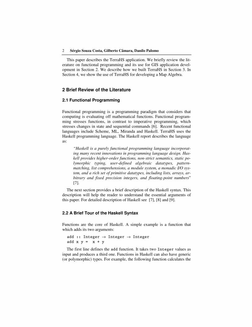
We define the Coverage data type to use the functions of the generic

type class Coverages. The Coverage data type is also parameterized.

data Coverage a b = Coverage ((a → b), [a])

The data type Coverage has two components:

• A coverage function that maps an object of generic type a to ge-

neric type b.

• A domain of objects of the polymorphic type a.

The instance of the type class Coverages to the Coverage data type is

shown below:

instance Coverages Coverage where

new_cov a f = (Coverage (f, a))

evaluate f o

| (elem o (domain f)) = Just ((fun f) o)

| otherwise = Nothing

domain (Coverage (f, a)) = a

num f = length (domain f)

values f = map (fun f) (domain f)

fun (Coverage (f,_)) = f

Figure 5 show an example of the Coverage data type.

c1 :: (Coverage String Integer) c1 = new_cov [”ab”,”abc”,”a”] length values c1 = [2,3,1] evaluate c1 “ab” = Just 2 evaluate c1 “ad” -- m1 not contain “ad” = Nothing

Fig.5.Example of use of the Coverage data type.


4.2 Operations

Câmara et al [19] define two classes of the map algebra operations: non-

spatial and spatial. For nonspatial operations, the value of a location in the

output map is obtained from the values of the same location in one or more

input maps. They include logical expressions such as “classify as high risk

all areas without vegetation with slope greater than 15%”, “Select areas

higher than 500 meters”, “Find the average of deforestation in the last

two years”, and “Select areas higher than 500 meters with temperatures

lower than 10 degrees”. Spatial functions are those where the value of a

location in the output map is computed from the values of the neighbor-

hood of the same location in the input map. They include expressions such

as “calculate the local mean of the map values” and “given a map of cities

and a digital terrain model, calculate the mean altitude for each city”. In

what follows, we show these operations in TerraHS, using polymorphic

data types.

4.2.1 TerraHS operations

Nonspatial operations are higher-order functions that take one value for

each input coverage and produce one value in the output coverage, using a

first-order function as argument. These include single argument functions

and multiple argument functions [19].

Spatial operations are higher-order functions that use a spatial predicate.

These functions combine a selection function and a multivalued function,

with two input coverages (the reference coverage and the value coverage)

and an output map [19]. Spatial functions generalize Tomlin’s focal and

zonal operations and have two parts: selection and composition. For each

location in the output coverage, the selection function finds the matching

region on the reference coverage. Then it applies the spatial predicate be-

tween the reference coverage and the value coverage and creates a set of

values. The composition function uses the selected values to produce the

result (Figure 6). Take the expression “given a map of cities and a digital

terrain model, calculate the mean altitude for each city”. In this expres-

sion, the value coverage is the digital terrain model and the reference cov-

erage is the coverage of cities. The evaluation has two parts. First, it se-

lects the terrain values inside each city. Then, it calculates the average of

these values.


Fig.6. Spatial operations (selection + composition). Adapted from [16].

In TerraHS, we use a generic type class for map algebra operations, as fol-

lows: class (Coverages cov) => CoverageOps cov where single :: (b → c) → (cov a b) → (cov a c) multiple:: ([b]→c)→ [(cov a b)] → (cov a b)→(cov a c) select :: (cov a b) → (a → c → Bool) → c → (cov a b) compose :: ([b] → b) → (cov a b) → b

spatial :: ([b] → b) → (cov a b) → (a → c → Bool)

→ (cov c b) → (cov c b)

The implicit assumption of these is that the geographical area of the output

coverage is the same as reference coverage. The instantiation of the cover-

age operations is provided by: instance CoverageOps Coverage where -- non-spatial operation on a single coverages single g c1 = new_cov (domain c1) ( g . (fun c1))

-- non-spatial operation on multiple coverages multiple fn clist c1 = new_cov (domain c1) (\x -> fn (faux clist x))

-- spatial selection select cov pr o = new_cov sel_dom (fun cov) where sel_dom = [l | l <- (domain cov), (pr l o)]

-- spatial composition compose f cov = (f (values cov))


-- spatial operation : selection + composition spatial fn c1 predic cref = new_cov (domain cref) (\x -> compose fn (select c1 predic x))

The single function has two arguments: a coverage and a first-

order function f. It returns a new coverage, whose domain is the same as

the input coverage. The coverage function of the output coverage is the

composition of the coverage function of the input coverage and the first-

order function g. Figure 7 shows an example of a single argument func-

tion.

single g c1 = new_cov (domain c1) ( g . (fun c1))

values c1 ⇒ [2, 4, 12] c2 = single square c1 values c2 ⇒ [4, 16, 144]

Figure 7 - Example of use of the single argument function

The multiple function has three arguments: a multivalued function, a

coverage list, and a reference coverage. It applies a multivalued function to

the coverage list. The result has thea same domain as the reference cover-

age. The new coverage function is defined using an auxiliary function that

scans the input list: multiple fn clist c1 = new_cov (domain c1) (\x -> fn (faux clist x))

For each location x of the reference coverage, the auxiliary function

faux applies the multiargument function in the input list of coverages. The

result is the output value for location x. The function faux handles cases

where there are multiargument function fails to returns an output value. faux :: (Eq a, Eq b, Coverages cov) => [(cov a b )] -> a -> [b] faux [] _ = [] faux (m:ms) e = faux1 (evaluate m e) where faux1 (Just v) = v : (faux ms e) faux1 (Nothing) = (faux ms e)


Figure 8 shows an example of multiple.

values c1 [2, 4, 8] values c2 ⇒ [4, 5, 10] c3 = multiple sum [c1, c2] c1 values c3 ⇒ [6, 9, 18]

Figure 8 - Example of use of multiple

The spatial selection has three arguments: an input coverage, a

predicate and a reference element. It selects all elements that satisfy a

predicate on a reference object (“select all deforested areas inside the state

of Amazonas”). select c prd o = new_cov sel_dom (fun c)

where sel_dom = [loc | loc ← (domain m) , (prd loc o)]

This function takes a reference element and an input coverage. It

creates a coverage that contains all elements of the input that satisfy the

predicate over the reference element. Figure 9 shows an example.

line= TeLine2D [(1,2),(2,2),(1,3),(0,4)] domain c1 ⇒ [TePoint (1,2),TePoint (2,3),TePoint (1,3)] c2 = select c1 intersects line domain c2 ⇒ [TePoint (1,2), TePoint (1,3)]

Figure 9 - Example of select.

The composition function combines selected values using a multi-

valued function. In Figure 10, the compose function is applied to coverage

c1 and to the multivalued function sum. compose f m = (f (values m))

values c1 ⇒ [2, 6, 8] compose sum c1 ⇒ 16

Figure 10 - Example of compose.


The spatial function combines spatial selection and composi-

tion. The output coverage has the same domain as the reference coverage.

For each location in the output coverage, the selection function produces a

set of values that satisfy a spatial predicate.. The composition function uses

the selected values to produce the result. Figure 11 shows an example.

spatial fn c prd cref = new_cov (domain cref) (\x → compose fn (select c prd x))

domain c1 = [TePoint (1,2),TePoint (2,3),TePoint (1,3)] values c1 = [4,5,10] domain c2 = [(TeLine2D[(1,2),(2,2),(1,3),(0,4)])] c3 = spatial sum c1 intersects c2 values m3 -- 4 + 10 = [14]

Figure 11 - Example of compose.

The spatial operation selects all points of c1 that intersect c2

(which is a single line). Then, it sums its values. In this case, points (1,2)

and (1,3) intersect the line. The sum of their values is 14.

4.3 Application Examples

In the previous section we described how to express the map algebra pro-

posed in Câmara et al. [19] in TerraHS. In this section we show the appli-

cation of this algebra to actual geographical data.

4.3.1 Storage and Retrieval

Since a Coverage is a generic data type, it can be applied to different con-

crete types. In this section we apply it to the Geometry and Value data

types available in the TerraHS, which represent, respectively, a region and

a descriptive value. TerraHS enables storage and retrieval of a geo-

object set. To perform a map algebra, we need to convert from a geo-

object set to a coverage and vice versa.

toCov::[GeObject]→ AttrName→ (Coverage Geometry Value) toGeObject::(Coverage Geometry Value)→AttrName →[GeObject]


Given a geo-object set and the name of one its attributes, the toCov function returns a coverage. Remember that a Coverage type has one

value for each region. Thus, a layer with three attributes it produce three

Coverages. The toGeObject function inverts the toCov function. De-

tails of these two functions are outside the scope of this paper. Given these

functions, we can store and retrieve a coverage, given a spatial database.

retrieveCov:: Database → LayerAttr → IO (Coverage Geometry Value) retrieveCov db (layername, attrname) = do db <- open db geoset <- retrieve db layername let cov = toCov geoset attrname close db return cov

The LayerAttr type is a tuple that represents the layer name and at-

tribute name. The retrieveCov function connects to the database, loads

a geo-object set, converts these geo-objects into a coverage, and return this

coverage as its output.

storeCov:: Database → LayerAttr→ (Coverage Geometry Value)→IO Bool storeCov db (layername, attrname) c1 = do let geos = toGeObject c1 attrname db <- open db close db let status = store db layername geos return status

The storeCov function coverts a coverage to a geo-object set that will

be saved in the database. We can now write a program that reads and

writes a coverage in a TerraLib database.

host = “sputnik” user = “Sergio” password = “terrahs” dbname = “Amazon” main:: IO () main = do db <- open (MySQL host user pass dbname)

def <-retrieveCov db (“amazonia”,“deforest")


-- apply a nonspatial operation

let defclass = single classify def storeCov db (“amazon”, “defclass”) defclass

Fig.12. Retrieving and storing a Coverage from a TerraLib Database

4.3.2 Examples of Map Algebra in TerraHS

Since 1989, the Brazilian National Institute for Space Research has been

monitoring the deforestation of the Brazilian Amazon, using remote sens-

ing images. We use some of this data as a basis for our examples. We se-

lected a data set from the central area of Pará, composed by a group of

highways and two protection areas. This area is divided in cells of 25 x 25

km2, where each cell describes the percentage of deforestation and defor-

ested area (Figure 14).

Fig.13. Deforestation, Protection Areas and Roads Maps (Pará State)

Our first example considers the expression: “Given a coverage of defor-

estation and classification function, return the classified coverage”. The

classification function defines four classes: (1) dense forest; (2) mixed for-

est with agriculture; (3) agriculture with forest fragments; (4) agricultural

area. This function is:


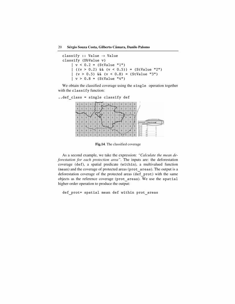
classify :: Value → Value classify (DbValue v) | v < 0.2 = (StValue "1") | ((v > 0.2) && (v < 0.5)) = (StValue "2") | (v > 0.5) && (v < 0.8) = (StValue "3") | v > 0.8 = (StValue "4")

We obtain the classified coverage using the single operation together

with the classify function:

..def_class = single classify def

Fig.14. The classified coverage

As a second example, we take the expression: “Calculate the mean de-

forestation for each protection area”. The inputs are: the deforestation

coverage (def), a spatial predicate (within), a multivalued function

(mean) and the coverage of protected areas (prot_areas). The output is a

deforestation coverage of the protected areas (def_prot) with the same

objects as the reference coverage (prot_areas). We use the spatial

higher-order operation to produce the output:

def_prot= spatial mean def within prot_areas


Fig.15. Deforest mean by protection area

In our third example, we consider the expression: “Given a coverage

containing roads and a deforestation coverage, calculate the mean of the

deforestation along the roads”. We have as inputs: the deforestation cov-

erage (def), a spatial predicate (intersect), a multivalued function

(mean) and a road coverage (roads). The product is a coverage with one

value for each road. This value is the mean of the cells that intercept this

road.

road_def= spatial mean def intersect roads

Fig. 16 Deforestation mean along the roads


5. Conclusions

This paper presents the TerraHS application for integrating functional pro-

gramming and spatial databases. We use TerraHS to develop and validate

a map algebra in a functional language. The resulting map algebra is com-

pact, generic and extensible. The example shows the benefits on using

functional programming, since it enables a fast prototyping and testing cy-

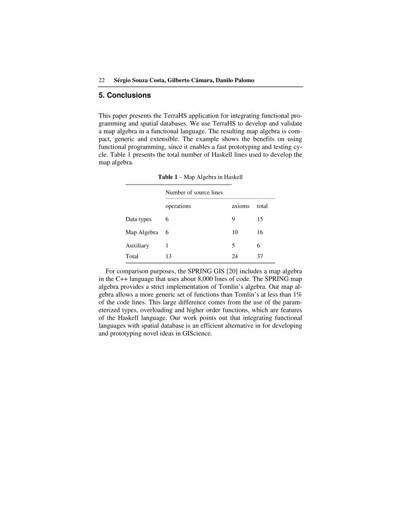
cle. Table 1 presents the total number of Haskell lines used to develop the

map algebra.

Table 1 – Map Algebra in Haskell

Number of source lines

operations axioms total

Data types 6 9 15

Map Algebra 6 10 16

Auxiliary 1 5 6

Total 13 24 37

For comparison purposes, the SPRING GIS [20] includes a map algebra

in the C++ language that uses about 8,000 lines of code. The SPRING map

algebra provides a strict implementation of Tomlin’s algebra. Our map al-

gebra allows a more generic set of functions than Tomlin’s at less than 1%

of the code lines. This large difference comes from the use of the param-

eterized types, overloading and higher order functions, which are features

of the Haskell language. Our work points out that integrating functional

languages with spatial database is an efficient alternative in for developing

and prototyping novel ideas in GIScience.


References

1. Frank, A. Higher order functions necessary for spatial theory development. in

Auto-Carto 13. 1997. Seattle, WA: ACSM/ASPRS.

2. Frank, A. and W. Kuhn, Specifying Open GIS with Functional Languages, in

Advances in Spatial Databases—4th International Symposium, SSD ‘95, Port-

land, ME, M. Egenhofer and J. Herring, Editors. 1995, Springer-Verlag: Ber-

lin. p. 184-195.

3. Frank, A. One Step up the Abstraction Ladder: Combining Algebras - From

Functional Pieces to a Whole. in COSIT - Conference on Spatial Information

Theory. 1999: Springer-Verlag.

4. Medak, D., Lifestyles - a new Paradigm in Spatio-Temporal Databases, in

Department for Geoinformation. 1999, Technical University of Vienna: Vi-

enna.

5. Winter, S. and S. Nittel, Formal information modelling for standardisation in

the spatial domain. International Journal of Geographical Information Sci-

ence, 2003. 17: p. 721--741.

6. Hudak, P., Conception, evolution, and application of functional programming

languages. ACM Comput. Surv., 1989. 21(3): p. 359-411.

7. Jones, S.P., Haskell 98 Language and Libraries The Revised Report. 2002.

8. Peyton Jones, S., J. Hughes, and L. Augustsson. Haskell 98: A Non-strict,

Purely Functional Language. 1999 [cited; Available from:

http://www.haskell.org/onlinereport/.

9. Thompson, S., Haskell:The Craft of Functional Programming. 1999, Harlow,

England: Pearson Education.

10. Chakravarty, M., The Haskell 98 foreign function interface 1.0: An addendum

to the Haskell 98 report. 2003.

11. Wadler, P., Comprehending monads, in Proceedings of the 1990 ACM con-

ference on LISP and functional programming 1990, ACM Press: Nice, France.

p. 61-78.

12. Jones, S.P., Tackling the Awkward Squad: monadic input/output, concur-

rency, exceptions, and foreign-language calls in Haskell. 2005.

13. Vinhas, L. and K.R. Ferreira, Descrição da TerraLib, in Bancos de Dados Ge-

ográficos, M. Casanova, et al., Editors. 2005, MundoGeo Editora: Curitiba. p.

397-439.


14. Chakravarty, A.P.a.M. Interfacing Haskell with Object-Oriented Lan-guage. in 15th International Workshop on the Implementation of Functional

Languages. 2004. Lübeck, Germany: Springer-Verlag.

15. Shields, M. and S.L.P. Jones, Object-Oriented Style Overloading for Haskell.

Electronic Notes in Theoretical Computer Science, 2001. 59(1).

16. Tomlin, C.D., A Map Algebra, in Harvard Computer Graphics Conference.

1983: Cambridge, MA.

17. Câmara, G., Representação computacional de dados geográficos, in Bancos de

Dados Geográficos, M. Casanova, et al., Editors. 2005, MundoGeo Editora:

Curitiba. p. 11-52.

18. OGC. Open GIS Consortium. Topic 6: the coverage type and its subtypes.

2000 [cited 2006 10/05/2006]; Available from:

http://portal.opengeospatial.org/files/?artifact_id=7198.

19. Câmara, G., et al. Towards a generalized map algebra: principles and data

types. in VII Workshop Brasileiro de Geoinformática. 2005. Campos do

Jordão: SBC.

20. Câmara, G., et al., SPRING: Integrating Remote Sensing and GIS with Ob-

ject-Oriented Data Modelling. Computers and Graphics, 1996. 15(6): p. 13-

22.

Documents

TerraHS: Integration of Functional Programming … · TerraHS: Integration of Functional Programming and Spatial Databases for GIS Application Development 3 length of a generic list,