Terra: system for land leveling projects with regular or

Revista Mexicana Ciencias Agrícolas volume 11 number 8 November 12 - December 31, 2020

1839

Article

Terra: system for land leveling projects with regular or variable topography

Francisco García Herrera1§

Jesús Chávez Morales1

Juan Enrique Rubiños Panta1

María Liliana Terrazas Onofre2

1Postgraduate College-Campus Montecillo-Hidrociencias. Mexico-Texcoco highway km 36.5, State of

Mexico. CP. 56230. Tel. 595 9520200. ([email protected]; [email protected]). 2Mexican College of

Natural Resources Specialists. From the flowers # 8, San Luis Huexotla, Texcoco, State of Mexico. CP.

56220. Tel. 595 9285236. ([email protected]).

§Corresponding author: [email protected].

Abstract

Land leveling is essential to reduce the volume of water applied and increase the uniformity of

gravity irrigation. The electronic computing system Terra is presented, for calculating agricultural

land leveling projects, useful for examining innumerable design alternatives in a very short period

of time. The field data with which it is fed, can be points obtained with a topographic survey of a

rectangular grid or a survey of variable distribution (radiation). The calculation of cut and fill

volumes is performed using ‘the four point method’ supported by the Kriging method in the case

of variable distribution topography. The algorithm developed is capable of dividing the land into

tables for independent leveling, with the aim of reducing cut and fill volumes, directly impacting

the leveling cost. Plans of the terrain topography are generated before and after leveling; plus cut

and fill plans and a block diagram as a guide for the operator in the leveling process.

Keywords: isolines, Kriging, MDE.

Reception date: June 2020

Acceptance date: September 2020

mailto:[email protected]




Rev. Mex. Cienc. Agríc. vol. 11 num. 8 November 12 - December 31, 2020

1840

Introduction

According to CONAGUA (2014) of the irrigation surface in Mexico, 90% has problems of low

application efficiencies, which can be improved with land leveling if the topographic slopes are

adequate, which implies greater uniformity of irrigation and a reduction of the volume of water

applied (Saucedo et al., 2006; Fuentes and Rendon, 2012).

Land leveling is justified in any irrigation project, since generally considerable sums are invested

in catchment and distribution works, comparatively low investments are made in the plot, which

is where the goodness of an entire complex irrigation system is reflected (Walker, 1987). Many

computer programs have been developed on the issue of leveling agricultural land, always

seeking to save time in design and perform optimal calculations with the lowest possible cost

(Covarrubias, 1968).

Among the first programs in Mexico there is Nivterra v1.0 developed for personal computers in

Fortran 77, with later improvements in Pascal for its version 2.0 (Chávez et al., 1990), giving rise

to systems that are used today in practice, such as the Sinivet in its different versions used for grid

surveys and for leveling without divisions (Hernández and Sánchez, 2008). The few programs

currently in existence for the design of land leveling projects use grid surveys as a data source.

As a result of several years of work in the area of software development applied to land leveling,

the Terra 1.0 program was developed to process field data obtained with topographic surveys with

the traditional survey method with points plotted on a grid rectangular or with a variable

distribution (radiation).

Terra, seeks to adapt to new technologies that involve the collection of information from field data,

for the use and application of land leveling. The objective was the development of an electronic

computing system, which includes topographic survey methods with modern equipment, such as

total stations or precision GPS, which helps in the precise and expeditious calculation for the

preparation of executive projects for leveling agricultural land.

Managing a mass of points taken by radiation instead of a grid implies generating a digital elevation

model (MDE) that describes the characterized property with high reliability. This is accomplished

on Terra using the Kriging method for terrain modeling.

Materials and methods

The methodology includes the application of spatial interpolation using the Kriging method

(Villatoro et al., 2008) for the determination of the weights or weighting factors in the calculation,

estimation and quantification of cut and fill volumes and plotting curves of ground level before and

after grading, covering areas that the surveyor does not do on a homogeneously spaced grid in the

traditional procedure.

The solution of the Kriging method allows the user to define a variogram of elevations based on

the best fit made to his experimental semivariogram (Clark, 1979). The models used to fit the

variograms are: linear, quadratic, spherical, exponential, and Gaussian, with or without the nugget


1841

effect (Delhome, 1978). Like Walker (1987); Cano (1997), Terra 1.0 includes the division of the

land into independent tables proposed by Marr (1957) in case the slopes of the land are

heterogeneous. In Figure 1, the algorithm used for the development of the Terra 1.0 system is

described in simplified form.

Figure 1. Leveling algorithm, implemented in Terra to calculate the project plan, without divisions

or in a single table.


1842

Definition of survey data

Depending on the type of topographic survey carried out, field coordinates were obtained for each

measured point, either in a rectangular grid using the proposal of Marr (1957), in which case they

are already coordinates (xi, yj, zij), where i=1, 2, …, n; j=1, 2, …, m; n= number of rows and m=

number of columns of the grid or radiations, in which case they are coordinates (Xrk, Yrk, Zrk).

Where: k= 1, 2,…, P and P= number of points raised by radiation; which will enter the program

dialog box, activating the corresponding capture option according to the survey carried out. In the

same way, the coordinates of each of the vertices of the terrain polygonal with their respective

coordinates (Xv,Yv) are entered. Where: v= 1, 2,…, NV and NV= number of vertices of the traverse

of the terrain.

Work limits, area and centroid

With the information of the captured field points, the extreme limits of a rectangular area are

determined for the leveling project work, defined by (Xmin,Ymin) in the lower left corner and

(Xmáx,Ymáx) in the upper right corner. In the case of a radiation survey, the nodes of a grid of

dimensions mxn are created in the defined rectangular area, with a distance between nodes

(Lcuadrícula), thus for each node there is information (xi, yj), missing estimating zij. With the

coordinates of the vertices of the traverse, the area and centroid of the terrain (xc, yc, zc) is

calculated.

Calculation of the project plan

This is carried out by ordinary least squares using a matrix solution such as that proposed by

Montgomery and Runger (2008), in which the way in which the topographic survey was carried

out is indistinct, the equation of the initial project plane is: zij=CA+CB xi+CC yj 1). Where: zij=

estimated elevation of the project plane at a coordinate point (xi, yj), in m; CA= constant that

geometrically represents the elevation of the project plane, at the origin of the coordinate

system, in m; CB= average slope of the terrain in the direction of the X axis, in dec; CC= average

slope of the terrain in the Y direction, in dec; xi= X coordinate of row i, in m; yj= Y coordinate

of column j, in m; i= 1, 2, 3, ..., n; j = 1, 2, 3, ..., m; n= number of rows; m= number of columns.

Guajarati and Porter (2010), propose to calculate the coefficients of a plane with: (AT A) β=

AT b 2); (A

T A)= [

1 1 1 … 1

X1 X2 X3 … Xn

Y1 Y2 Y3 … Yn

]

[ 1 X1 Y1

1 X2 Y1

1 X3 Y1

⋮ ⋮ ⋮1 Xn Yn]

3);

(AT b)= [

1 1 1 … 1

X1 X2 X3 … Xn

Y1 Y2 Y3 … Yn

]

[ Z1

Z2

Z3

⋮Zn]

4)

Where: A = matrix of XY coordinates; AT = transpose of the XY coordinate matrix; b= Z coordinate

vector; β= vector of unknowns or coefficients (CA, CB, CC). From equation (2) the vector of


1843

unknowns or vector of coefficients (β) is cleared, to obtain the values of the slopes of the plane (CB

and CC) and the ordinate to the origin (CA): β = (AT A)

-1(A

T b) 5); β= [

β1

β2

β3

] = [CA

CB

CC

] 6).

Homogeneous grid calculation

If the survey was by means of a grid, it was already drawn in the field when doing the topographic

survey, but if it was by radiation, the grid is created from the limits previously calculated and with

a regular equidistance from the grid assigned for the size calculation. Lcuadricula (m), which can be

the same as the regular grid or another as the case may be. This defines the number of nodes in X

and Y (Figure 2).

Figure 2. Elements to determine the homogeneous grid, from a topographic survey by radiation and

an MDE.

The problems that were detected at this point are due to having very short fields where only one

line can be defined, and therefore, no frame can be generated, the most practical solution is to

redefine a smaller value of the Lcuadricula. With the above information, it is possible to determine the

location (xi, yj) of each node within the grid.


1844

Determination of the coordinates zij

In each node (i, j) of the grid, the values of zij are determined through a geostatistical process

of spatial interpolation, starting from the information collected in the field (Xrk, Yrk, Zrk) of

the field data defined as neighboring points to the node (i,j). The definition of neighboring

points is performed by calculating the distance from each node (i, j) to all the coordinates

obtained in the topographic survey (Xrk, Yrk, Zrk), the NC points with the smallest distances

will make up the set of neighboring points or close for the estimation of zij, using equation (7).

zij= ∑ Wq ZqNCq=1 7).

Where: zij= estimated data at node (i, j) of the generated grid of mxn dimensions; i = 1, 2, 3, n; j

= 1, 2, 3, ..., m; n= number of rows; m= number of columns. Zq= Zrk coordinate of the field point

located at position q of the set of neighboring or nearby points. Wq= weight or weighting factor

calculated for the site q of the set of neighboring or close points for the estimation of zij at node

(i, j). NC= total number of points near or near the node (i, j), which will be used to estimate the

data zij. The sum of the values of the weights or weighting factors (Wq) of the set of points near or

close to the node (i, j) must meet the restriction defined in equation (8): ∑ WqNCq=1 =1 8).

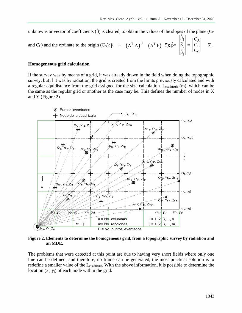
Calculation of the weights or weighting factor (Wq)

The calculation of the weights is carried out by applying the Kriging method. Clayton and Andre

(1998) indicate that the essence of Kriging is the estimation of the semivariogram (Figure 3), in

this case of elevations, which is constructed by defining 20 classes of distances with all field data

(P) and calculating γ (h) for each class located at a distance (dt+h) the value of the semivariogram γ

(h) through equation 9. γ(h)= ∑ [Zr(dt)-Zr(dt+h)]2P

t=1

2P 9).

Figure 3. Topography of the natural terrain, applying the Kriging method, in a topographic survey

with variable radiation distribution.


1845

Where: Zr(dt)= value of the topography elevation (Z) at point t; Zr(dt+h)= value of the topographic

elevation (Z) at the site located at distance h from point t; P= total number of points in the

radiation survey.

Once the semivariogram is calculated for each of the distances defined in the classes, a theoretical

model is adjusted (Cisneros-lturbe et al., 1999), which can be: linear, quadratic, spherical,

exponential or Gaussian (Table 1) equations 10, 11, 12, 13 and 14.

Table 1. Mathematical models (Delhome, 1978; Clark, 1979), available in Terra for fitting the

theoretical variogram, from the experimental semivariogram.

Model Function for (0 < h ≤ C2) and linearization

Linear γ(h)= C1h (10)

Quadratic γ(h)= C1 [2 (

h

C2

) - (h

C2

)2

]

γ(h)= β1h+ β

2h

2

(11)

(11a)

Spherical γ(h)= C1 [

3

2(

h

C2

) -1

2(

h

C2

)3

]

γ(h)= β1h+ β

2h

3

(12)

(12a)

Exponential (*) γ(h)= C1 [1-exp (-

h

C2

)]

γ(h)≅ C1 [1-5

2 e] +

2

e(C1

C2

) h-1

2 e(

C1

C22) h

2 (*)

γ(h)≅ β0+β

1h+ β

2h

2

(13)

(13a)

(13b)

Gaussian (*) γ(h)= C1 [1-exp (-

h

C2

)2

]

γ(h)≅ C1- (4 C1

e) + (

4 C1

e C2

) h- (C1

e C22) h

2 (*)

γ(h)≅ β0+β

1h+ β

2h

2

(14)

(14a)

(14b)

When h>C2: C = (h) 1 (for Quadratic and Spherical models)(*) function approximated to polynomial, using Taylor series

and for h= C2.

Michael and Clayton (2014), mention that the behaviors at the origin of the models may or may

not consider the nugget affect; that is, the intersection with the Y axis or, consider that they leave

the origin, as is the case with topography. Initially, it was tested with varigram models that include

the nugget effect; however, most solutions implied negative values for the coefficient C0, which is

why it was decided to use the model that comes from the origin (Legra-Lobaina et al., 2010).

The calculation of the coefficients of the models (C0, C1 and C2) was done with the Newton-

Raphson method for the solution of systems of non-linear equations (Chapra and Canale, 2015),

with unfavorable results, therefore, the models were linearized (Table 1) equations 11a, 12a, 13b

and 14b, improving the solutions.


1846

Before linearization, the exponential and Gaussian models were approximated to a polynomial

function (equations 13a and 14a), using Taylor series (Purcell and Varberg, 2009). Once the

models were linearized, equation (5) was applied to determine the βi coefficients and for the

calculation of the C1 and C2 coefficients of the variogram, the solutions are listed in (Table 2)

equations 15 to 20b.

Table 2. C1 and C2 coefficients, obtained to determine the theoretical variogram.

Model Coefficients for variograms starting from the origin (C0= 0)

C2 (rank) C1 (Sill)

Quadratic C2=-0.5 (

β1

β2

⁄ )

(15) C1=-0.25 (β

1

2

β2

⁄ )

(15a)

Spherical

C2=0.58143 √-β

1β

2

⁄

(16)

C1=0.66667 β1 C2

(16a)

Exponential C2=-0.25 (

β1

β2

⁄ )

C2=1.51348 √-β

0β

2

⁄

(17)

(18)

C1=-0.33979 (β

1

2

β2

⁄ )

C1=12.45308 β0

(17a)

(18a)

Gaussian C2=-0.25 (

β1

β2

⁄ )

C2=-3.12081 (β

0β

1

⁄ )

(19)

(20)

C1=-0.16989 (β

1

2

β2

⁄ )

C1=2.12081 β0

(19a)

(20a)

Once the coefficients of the theoretical variogram have been calculated, the estimation of the

weights or weighting factors (Wq) for each of the nodes is done through a matrix process (equations

21, 22 and 23).

Sw= b 21) S=

[ γ

11γ

12⋯ γ

1n1

γ21

γ22

⋯ γ2n

1

⋮ ⋮ ⋱ ⋮ ⋮γ

n1γ

n2⋯ γ

nn1

1 1 ⋯ 1 0]

; w=

[ W1

W2

⋮Wn

λ ]

; b=

[ γ

1γ

2

⋮γ

n

1 ]

22)

Where: S= is a square matrix of order n x n; each element of the matrix is calculated by evaluating

the theoretical variogram with the distance between points; for example: the element 𝛾12 is

calculated by evaluating the variogram function with the existing distance between point 1 and 2

of the NC close or neighboring points that were involved for the interpolation process. W and b=

are the vectors of order n x 1.

The vector b is obtained by evaluating the function of the variogram with the distance between the

node (i, j) where zij will be estimated and the neighboring data q. w contains the n unknowns

involved in the calculation; that is, the weights of each of the NC data, plus a Lagrange multiplier


1847

(λ) that stores the residual error calculated in the process, thus clearing the vector w will obtain the

weights or weights sought (Wq).w= S-1b (23). As a product of this step, a file (*.MLL) is obtained

with the zij information for each of the nodes of the homogeneous grid.

Adjusting the ordinate to origin (CA)

The adjustment of the ordinate to the origin (CA) of the project plan calculated in the second step

is carried out according to the relationship between the cuts and fills defined by the abundance

coefficient (R= cut/fill), most authors agree that the abundance coefficient (R) must be in the range:

1.1 ≤ R ≤ 1.5 (Walker 1988).

In practice, where there were fillings, there will be compaction and holes will remain, these will

appear over time due to rain and soil compaction, so it is necessary to increase the cuts, therefore

the fillings will decrease, this is done until have a coefficient of abundance (R) within the desired

range, the adjustment is made by lowering or raising the project plane in ±Δh, h is the value of

increase or decrease in the elevation of the plane in m, depending on the ground and its greater or

lower content of organic matter.

That is, if a soil is sandy the coefficient R will be close to 1.1, clay the value of the coefficient

will be close to 1.5. If an intermediate soil (clay loam) is considered, the coefficient values will

vary between 1.20 and 1.30 (Walker, 1988). The calculation of the cut and fill volumes is done

using the 4-point method; it is necessary to have a grid with field data or generated by the

Kriging method.

The incorporation of the Kriging method for estimating the elevation (zij) at each node (i, j) of the

grid is a new procedure in land leveling and has shown technically adequate results in the

calculation of volumes of land. cut and fill. As a result of the step, an adjusted CA coefficient (CAajus)

is obtained for the equation of the project plan. With the above, final values of cut or fill thicknesses

are calculated for each node (i, j) of the grid and therefore cut and fill volumes, as well as leveling

costs per hectare and total.

Generation and drawing of isolines

Contour drawings are drawn for the natural terrain (pre-grading setup) and for the graded

terrain project (post-grading setup). This process is carried out in two ways: a) contour lines

are created for the entire terrain, regardless of how the topographic survey was carried out, a

new, finer grid (x’i, y’j, z’ij) generated with Smallest inter-node lengths, about a quarter the

length of the grid for leveling.

This new grid is calculated from the field data collected in a rectangular grid (xi, yj, zij) or by

radiation (Xrk, Yrk, Zrk) applying the spatial interpolation process with the Kriging method

explained in the previous points or the inverse distance method. The limits of the new grid are

extended to perfectly cover the traverse of the terrain and avoid areas without curves. The

calculation and drawing of isolines or level curves of the leveled terrain is carried out with the

nodes (i, j) of the new grid, whose elevation zij is obtained with the final equation, equation (1)


1848

defined for the project plan; and b) in the event that due to abrupt changes in slopes or lot size

it is necessary to divide the land, to make its independent leveling by tables, an algorithm was

designed that allows the property to be divided into two parts interactively with the user.

The example shows the topography of the natural terrain so that a dividing line can be drawn on it

that allows separating the points raised in the new polygons and natural project planes, which result

with the dividing line. In case you need to divide the property into more than two parts, you have

a capture form to define the polygons.

The latter in order for the designer to manually identify the limits of the polygons and with this all

the points surveyed in the field remain inside. Once the tables have been defined, the six points

described above will be applied to calculate the natural project and final plan, as well as the

calculation of cut and fill volumes independently of each of the tables.

Results and discussion

Terra 1.0 was developed with the Delphi (Pascal) programming language, designed to function as

a tool in any land leveling project where the topography is raised in a grid with rectangular lines or

radiations. The system allows the general leveling of the entire raised property or the division by

tables.

The calculation of cut and fill volumes is performed with the rectangular grid applying the Kriging

method for the calculation. The estimation of the values of the grid generates values congruent with

the topography and therefore the calculation of volumes is obtained according to the pre-

established technical procedures.

Information capture

Terra has three dialog boxes to capture the input information: ‘project data and design parameters’

for general data, ‘terrain traverse data and centroid calculation’ to capture the coordinates (Xv, Yv)

of the vertices of the terrain traverse and ‘topographic data for leveling’, for field data with

coordinates (xi, yj, zij) or (Xrk, Yrk, Zrk) according to the topographic survey carried out and the

length of equidistance from the grid.

Natural terrain topography

The program allows the generation and visualization of the terrain topography with contour lines

(Figure 6). In order to draw them, a digital elevation model has been calculated using the Kriging

method. According to Delhome (1979), he recommends the use of the Kriging method in

applications to hydroscience, indicating that it adequately describes the behavior of the natural

terrain topography. The initial proposal for the calculation of the coefficients C0 and C1 of the

theoretical variogram model is automatically adjusted to the linear model; however, you can choose

another one in a personalized way (Figure 3).


1849

Figure 6. Level curve planes of leveled terrain cut and fill values at grid nodes and earthwork block

diagram.

Topographic survey in rectangular grid

The software developed allows processing the information obtained with a survey with a

rectangular grid, so the traditional methodology can be applied to calculate land leveling. In this

case, the field grid already exists so there is no need to create a new one. As is the case of radiation

survey where the grid is generated.

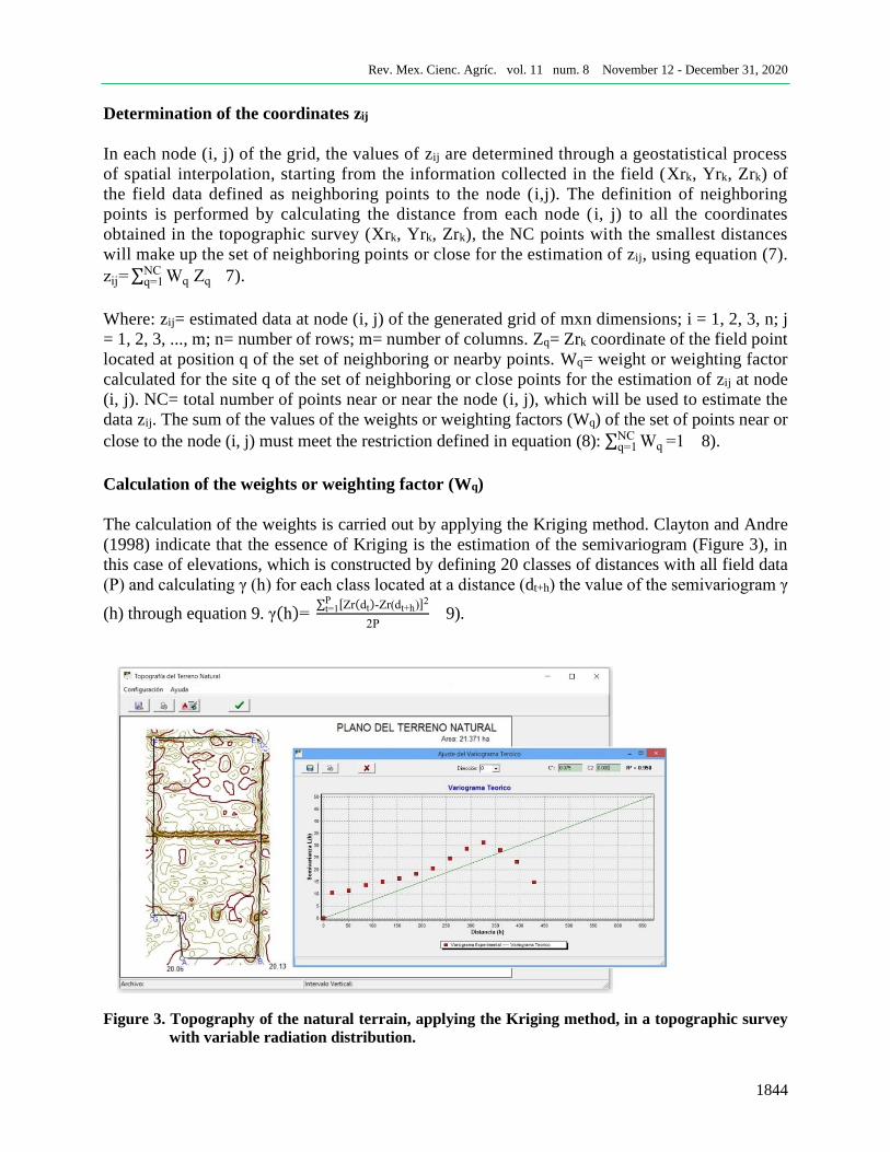
Division of the terrain in tables

The software developed allows the terrain to be divided into two tables, drawing a dividing line

and generating the two independent polygons automatically (Figure 4). When a radiation

survey is carried out, some points are taken close to the limits and with a high probability they

can fall out of the ground, the system assigns all the points in one of the two polygons; however,

when the division involves a greater number of parts, it will be very difficult to group the

points, which is why there is an information entry sheet where the user must enter the

coordinates of each polygon and for each table only it will extract the information that is within

the defined polygon.

Once the division of the land has been carried out, each defined table is analyzed separately.

In the example, leveling was carried out by tables, making a dividing line in the middle part of

the terrain where it can be clearly seen that there is a sudden change in slope, seeking to reduce

the cutting and filling volumes and therefore the total cost of leveling (Figures 4 and 5).


1850

Figure 4. Division of the land in independent tables.

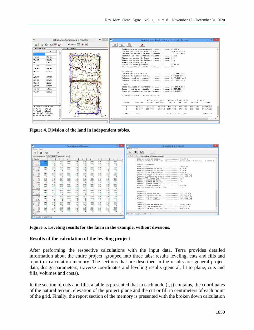
Figure 5. Leveling results for the farm in the example, without divisions.

Results of the calculation of the leveling project

After performing the respective calculations with the input data, Terra provides detailed

information about the entire project, grouped into three tabs: results leveling, cuts and fills and

report or calculation memory. The sections that are described in the results are: general project

data, design parameters, traverse coordinates and leveling results (general, fit to plane, cuts and

fills, volumes and costs).

In the section of cuts and fills, a table is presented that in each node (i, j) contains, the coordinates

of the natural terrain, elevation of the project plane and the cut or fill in centimeters of each point

of the grid. Finally, the report section of the memory is presented with the broken down calculation


1851

of the results: the matrix solution of the system of equations to calculate the project plan, the

calculation of the area, centroid and centroidal height, the initial project with the topographic

information and of the project plan, the calculation of the equation of the plan and the iterations for

the adjustment of the plan (Figure 5).

Calculation and generation of isolines

With Terra you can calculate and draw representative contour lines of the analyzed grid. To do

this, the isolines are created in two different ways: the first with the field data obtained in the

topographic survey by grid, the second through the geostatistical procedure of spatial

interpolation detailed in the previous sections, with which a grid is created with one of two

methods: the Kriging method or the inverse of distance method. Also presented is a cut and fill

plan and a cut and fill block diagram that serves as a guide to the operator for leveling work in

the field (Figure 6).

Cost estimation

The total leveling cost for the example of figures 4 and 5, whose summary is shown in Table

3, had a reduction of 43%, from $65 114.14 to $36 987.43 considering the cost m-3 of

earthworks in $20.80, by dividing the terrain into two tables based on the topography of the

natural terrain, which improved the initial design without divisions, considering only average

natural slopes.

Table 3. Comparison of volumes and costs for the example, applying the leveling to the entire

land vs the property divided into two tables according to topography of the natural land.

No.

Area(ha)

Volume ha (m3) Volume total (m3) Cost ($)

Tables Cut Filling Cut Filling Per

hectare Total

1 21.371 146.48 115.987 3 130.4874 2478.8105 3 046.776 65 114.137

2 21.371 1 778.242 1 377.892 36 987.43

11.215 57.144 45.057 640.859 505.309 1 188.597 13 329.875

10.157 111.984 85.912 1 137.382 872.583 2 329.261 23,657.555

The value of 1 in no. tables, indicates that the land was not divided.

One of the most important technical aspects of this work is the generation of the digital elevation

model through the Kriging method, for the determination of cut or fill heights and quantification

of cut and fill volumes, where the method of the four points suggested by the United States

Department of Agriculture (1970) and which applies for its estimation a grid whose area of

influence is a square. To ensure that the Terra model is technically adequate, the DEM was

compared with a professional program such as Surfer (Golden software, 2011), the generated

models are shown in Figure 7.


1852

Figure 7. Digital elevation models generated by Surfer and Terra, for the example.

The models consist of 39 columns and 73 rows, with a total of 2847 Z elevation data, with means:

Zm- Terra= 20.00739094, Zm-SURFER= 20.0099793 and variances: S²- Terra= 0.00373831, S²-

SURFER: 0.0038837, when performing a statistical test for means different and different variances,

it was concluded that the previous models with 97% reliability have equal mean values and with a

99% reliability value they have similar variances, which makes us conclude that they are practically

equal.

This allows us to assert that the model generated by Terra, predicts the behavior in an adequate

way and therefore, when generating the grid to estimate the values of cuts and fills, it generates

congruent volumes that allow to adjust the project plane of the leveling in an appropriate way. With

the application of modern technologies for land leveling, such as leveling with laser beam, the

development of a leveling project seems unnecessary.

However, this is not the case; any leveling project, regardless of the way the field data is taken,

needs an executive project with data and results that include a calculation memory with the

estimation of cut and fill volumes and of course the cost of leveling, the plan with the original

topography and level terrain. This will be the sustenance of the project and the support for the user

to carry out the necessary procedures in case of requiring financial support in institutions that

provide it to the field or in the payment of the earthworks to the tractor operator who carries out

the work, without any doubt.

Conclusions

Terra 1.0, which is presented, is an electronic computing system developed as a fundamental tool

to assist technicians in the formulation and optimization of executive projects for land leveling. It

includes algorithms for calculating the project from a topographic survey carried out in a grid or

with a variable distribution.

The use of the Kriging method was successfully integrated for the calculation of the isolines of

the plane of the natural terrain, of the leveled terrain, and the use of a raised or generated grid

that allows the calculation of the volume of cuts and fills. The methodology used involved


1853

solving in detail the ordinary least squares fit using a matrix method for the calculation of the

initial plane and implementing an efficient algorithm for the adjustment of the CA coefficient

of the plane equation.

In the case of the generated grid, algorithms are included for the determination of semivariograms

and algebraic equations were proposed for the calculation of the coefficients C1 and C2 of the

theoretical variogram, for the calculation of the weights in the spatial interpolation of the data of

the grid. In the case of the division into tables or terraces, algorithms were implemented to separate

the field points according to the divided polygons; the necessary routines are included so that the

designer can generate a technically adequate design of the leveling, thereby reducing the total

volumes of cuts and fillings and therefore reducing leveling costs. The Terra system can be used

with the point clouds that are generated in topographic surveys that are carried out with VANTs,

known as drones.

Cited literature

Cano-Muñoz, J. y Vázquez-Guzmán, A. 1997. Nivelación de tierras. Ediciones Mundi-Prensa.

Ministerio de Agricultura, Pesca y Alimentación, Sevilla, España. 215 p.

Cisneros-lturbe, H. L.; Bouvier, C. y Domínguez-Mora, R. 1999. Aplicación del método Kriging

en la construcción de campos de tormenta en la ciudad de México. Ingeniería Hidráulica

en México. 16(3):5-14.

Clark, I. 1979. Practical geostatistics. Cuarta reimpresión. (Ed.). Elsevier Applied Science.

London, Great Britain. 127 p.

Clayton, V. D. and André, G. J. 1998. GSLIB: geoestatistical software library and User’s Guide.

Oxford University Press, New York, USA. 369 p.

CONAGUA. 2014. Subdirección General de Infraestructura Hidroagrícola. Gerencia de Distritos

de Riego. Proyecto de riego por gravedad tecnificado (RIGRAT). Curso de capacitación:

Nivelación de tierras para el riego por gravedad. México, DF. 132 p.

Covarrubias-Lugo, A. 1968. Cálculo de nivelación de tierras para riego por medio del cómputo

electrónico. Ingeniería Hidráulica. México, DF. 80 p.

Chapra, C. S. y Canale, R. P. 2015. Métodos Numéricos para Ingenieros. Editorial Mc Graw Hill.

Séptima Edición. México, DF. 500 p.

Chávez-Morales, J.; Ibañez-Castillo, L. A. y Hernández-Saucedo, F. R. 1990. Programa de

nivelación de tierras (NIVTERRA 1.1). Colegio de Postgraduados, Hidrociencias.

Montecillo, México. 25 p.

Delhome, J. P. 1978. Kriging in the hydrociencies. Advances in water resouces.1(5):251-266.

Fuentes-Ruiz, C. y Rendón-Pimentel, L. 2012. Riego por gravedad. Universidad Autónoma de

Querétaro-CONAGUA. 358 p.

Guajarati, D. N. y Porter, D. C. 2010. Econometría. (Ed.). Mc Graw Hill. Quinta Edición. México,

DF. 801-876 p.

Hernández-Saucedo, F. R y Sánchez-Bravo, J. R. 2008. Manual para diseño de obras de riego

pequeñas. Capítulo 1.4: Nivelación de Tierras. Editado por: De León, M. B. y Robles, R.

B. D. Instituto Mexicano de Tecnología del Agua (IMTA). Jiutepec, Morelos. 53-73 p.

Legrá-Lobaina, A. A. y Atanes-Beatón, D. M. 2010. Variogramas adaptativos: un método práctico

para aumentar la utilidad del error de estimación por Kriging. Minería y Geología.

26(4):53-78.


1854

Marr, J. C. 1957. Grading land for surface irrigation. University of California, Division of

Agricultural Sciences. Davis, USA. Circular 438. 55 p.

Michael, J. P. y Clayton, V. D. 2014. Geostatistical reservoir modeling. Second Edition. Oxford

University Press. New York, USA. 362 p.

Montgomery, D. C. y Runger, G. C. 2008. Probabilidad y estadística aplicadas a la ingeniería.

Editorial Limusa Wiley. 2da. (Ed.). México, DF. 430-560 pp.

Purcell, E. J y Varberg, D. 2009. Cálculo con geometría analítica. Editorial Prentice Hall

Hispanoamericana, SA. 9ª Edición. México, DF. 451 p.

Saucedo, H.; Fuentes, C. y Zavala, M. 2006. El sistema de ecuaciones de Saint-Venant y Richards

del riego por gravedad: 3. Verificación numérica de la hipótesis del tiempo de contacto en

el riego por melgas. Ingeniería Hidráulica en México. 21(4):135-143.

US. 1970. Department of Agriculture, Soil Conservation Service. Land leveling, national

engineering handbook. US. Government Printing Office. Washington, DC. Chap 12:65 p.

Villatoro, M.; Henríquez, C. y Sancho, F. 2008. Comparación de los interpoladores IDW y

Kiging en la variación espacial de PH, CA, CICE y P del suelo. Agron. Costarricense.

32(1):95-105.

Walker, W. R. and Skogerboe, G. V. 1987. Surface irrigation: theory and practice. Editorial

Prentice-Hall. A Division of Simon and Schuster. Englewood Cliffs, New Jersey, 07632

USA. 178-191 pp.

Documents

Terra: system for land leveling projects with regular or