Embed Size (px)
Citation preview
Terminal Control of a Variable-Stability Slender Reentry
Vehicle
by
Matthew Thomas Karmondy
B.S., Aeronautical EngineeringUnited States Air Force Academy, 2006
Submitted to the Department of Aeronautics and Astronautics in Partial Ful�llmentof the Requirements for the Degree of
MASTER OF SCIENCEat the
MASSACHUSETTS INSTITUTE OF TECHNOLOGY June 2008
c©Matthew T. Karmondy, 2008. All rights reserved.
The author hereby grants to MIT permission to reproduce and to distribute publiclypaper and electronic copies of this thesis document in whole or in part in any
medium now known or hereafter created.
Signature of the Author . . . . . . . . . . . . . . . . . . . . . . . . . . . . . . . . . . . . . . . . . . . . . . . . . . . . . . . . . . .Department of Aeronautics and Astronautics
May 23, 2008
Certi�ed by . . . . . . . . . . . . . . . . . . . . . . . . . . . . . . . . . . . . . . . . . . . . . . . . . . . . . . . . . . . . . . . . . . . . . . .John J. Deyst, Jr.
Professor of Aeronautics and AstronauticsThesis Advisor
Certi�ed by . . . . . . . . . . . . . . . . . . . . . . . . . . . . . . . . . . . . . . . . . . . . . . . . . . . . . . . . . . . . . . . . . . . . . . .Laurent Duchesne
Charles Stark Draper Laboratory Thesis Supervisor
Accepted by . . . . . . . . . . . . . . . . . . . . . . . . . . . . . . . . . . . . . . . . . . . . . . . . . . . . . . . . . . . . . . . . . . . . . .Prof. David L. Darmofal
Associate Department HeadChair, Committee on Graduate Students
Report Documentation Page Form ApprovedOMB No. 0704-0188
Public reporting burden for the collection of information is estimated to average 1 hour per response, including the time for reviewing instructions, searching existing data sources, gathering andmaintaining the data needed, and completing and reviewing the collection of information. Send comments regarding this burden estimate or any other aspect of this collection of information,including suggestions for reducing this burden, to Washington Headquarters Services, Directorate for Information Operations and Reports, 1215 Jefferson Davis Highway, Suite 1204, ArlingtonVA 22202-4302. Respondents should be aware that notwithstanding any other provision of law, no person shall be subject to a penalty for failing to comply with a collection of information if itdoes not display a currently valid OMB control number.
1. REPORT DATE 02 JUN 2008
2. REPORT TYPE N/A
3. DATES COVERED -
4. TITLE AND SUBTITLE Terminal Control of a Variable-Stability Slender Reentry Vehicle
5a. CONTRACT NUMBER
5b. GRANT NUMBER
5c. PROGRAM ELEMENT NUMBER
6. AUTHOR(S) 5d. PROJECT NUMBER
5e. TASK NUMBER
5f. WORK UNIT NUMBER
7. PERFORMING ORGANIZATION NAME(S) AND ADDRESS(ES) Massachusetts Institute of Technology
8. PERFORMING ORGANIZATIONREPORT NUMBER CI08-0014
9. SPONSORING/MONITORING AGENCY NAME(S) AND ADDRESS(ES) The Department of the Air Force AFIT/ENEL, Bldg 16 2275 D StreetWPAFB, OH 45433
10. SPONSOR/MONITOR’S ACRONYM(S)
11. SPONSOR/MONITOR’S REPORT NUMBER(S)
12. DISTRIBUTION/AVAILABILITY STATEMENT Approved for public release, distribution unlimited
13. SUPPLEMENTARY NOTES The original document contains color images.
14. ABSTRACT
15. SUBJECT TERMS
16. SECURITY CLASSIFICATION OF: 17. LIMITATION OF ABSTRACT
UU
18. NUMBEROF PAGES
137
19a. NAME OFRESPONSIBLE PERSON
a. REPORT unclassified
b. ABSTRACT unclassified
c. THIS PAGE unclassified
Standard Form 298 (Rev. 8-98) Prescribed by ANSI Std Z39-18

Terminal Control of a Variable-Stability Slender Reentry Vehicle
by
Matthew Thomas Karmondy
Submitted to the Department of Aeronautics and Astronautics on May 23, 2008 inPartial Ful�llment of the Requirements for the Degree of Master of Science in
Aeronautics and Astronautics.
ABSTRACTVarious terminal control schemes are applied to a proposed slender reentry vehicle,controlled by two separately-articulating �aps. The �ap de�ections are summarizedas symmetric and asymmetric �ap de�ections; the former manipulates the drag, lift-curve slope, and static margin; the latter controls the vehicle trim characteristics.The control problem is interesting because the static margin can be actively con-trolled from statically stable in pitch to statically unstable in pitch. De�ection limitson the �aps present a control saturation that must be considered in control systemdesign. A baseline, angle of attack tracking linear-quadratic servo (LQ-servo) con-troller is detailed, including an analysis of actuator dynamics and a lead compensator.Desired time response characteristics and robustness to center of pressure uncertainty,reduced control e�ectiveness, and external pitch accelerations drive the selection of asymmetric de�ection at speci�ed points on the reentry trajectory. A hybrid switching-linear controller (SLC) is developed to reduce the peak overshoot and settling time.A saturated control drives the phase plane trajectory toward a region of satisfactorylinear control, where the LQ-servo controller is properly initialized and controls thephase plane trajectory to the reference command. SLC does not provide appreciablerobustness gains compared to the LQ-servo controller. A model-reference adaptivecontroller is described. Saturation e�ects prevent the adaptive controller from pro-viding additional robustness. A method to adaptively control both the symmetricand asymmetric �ap de�ections is proposed.
Thesis Advisor: John J. Deyst, Jr., Professor of Aeronautics and AstronauticsThesis Supervisor: Laurent Duchesne, C.S. Draper Laboratory
3

This page intentionally left blank.

Acknowledgments
It really is amazing that two years have already passed and I have a complete thesissitting in front of me. Although I am not totally convinced my research will changethe face of aerospace engineering (although all graduate students secretly hope theirwork will), the MIT/Draper experience was incredible. Moreover, I am indebted toeveryone who helped all along the way to the �nal publication the 100-plus page�What I Did for Two Years in Boston.� I cannot thank you all enough for yourtechnical expertise, moral support, and constant reassurance that pilot training isnot too far o�.
Laurent Duchesne must be thanked �rst. His guidance, from the most basicclassical control strategy, through the murky waters of discrete signal processing, toour vain attempts at a µ controller, was truly the cornerstone upon which I builtmy two years of research. Despite my relative inexperience in controls engineering,Laurent was inordinately helpful in narrowing the formidable �eld of �high-speedcontrol� to a workable, Master's Degree thesis. His constant demand to ensure wereally understood the problem is probably the primary reason I am pleased with my�nal thesis�it is not a mess of math and theory, but rather a logical (if technical)solution to an exciting problem. Naturally, the aid of Professor John Deyst must berecognized, too. From the �rst time I approached Professor Deyst, his excitementabout the problem was contagious. His vast experience in controls was a veritablefountain of ideas that, given another 5 years, I still would never have even imagined.The degree of autonomy he provided, combined with his keen insight, helped megenerate a �nal product of which I am proud.
The Draper sta� provided such a huge measure of support, and I cannot thankthem enough. Sean George and his aerodynamic knowledge at our weekly meetingshelped tame the wild woods of hypersonics. My Division Leader, Dr. Brent Appleby,ensured all us Draper Fellows were set up for success from Day 1. And of course, theother fellows here. The assistance with classes, enlightened discussions about thesiswork, the occasional griping followed by a moment of realization, and the �controls-free� lunches kept me sane (and kept me from failing out).
5

Where would I be without the other lieutenants here? Without you guys,nothing would have broken up the monotony of classes and MATLAB code. Most ofall, I have got to hand it to my roommate. Living with me through the ups and downsof MIT, research, and squirrels in the wall probably quali�es you for an award...I'llwork on that paperwork.
Finally, my family provided constant support (and dinner recipes). Sundaynight always seemed a little less daunting knowing I would be talking to you ratherthan hiding from Monday's looming head.
This thesis was prepared at the Charles Stark Draper Laboratory, Inc., underContract N00014-06-D-0171 for the O�ce of Naval Research.
Publication of this thesis does not constitute approval by Draper or the spon-soring agency of the �ndings or conclusions contained herein. It is published for theexchange and stimulation of ideas.
The views expressed in this thesis are those of the author and do not re�ect theo�cial policy or position of the United States Air Force, the Department of Defenseor the United States Government.
�����������������Matthew T. Karmondy, 2d Lt, USAF
23 May 2008
6

Contents
List of Figures 13
List of Tables 21
Nomenclature 23
1 Background 27
1.1 Motivation . . . . . . . . . . . . . . . . . . . . . . . . . . . . . . . . . 27
1.2 Research Objectives . . . . . . . . . . . . . . . . . . . . . . . . . . . . 29
1.3 Thesis Organization . . . . . . . . . . . . . . . . . . . . . . . . . . . . 30
7
2 Problem Formulation 33
2.1 Vehicle Aerodynamics Model . . . . . . . . . . . . . . . . . . . . . . . 33
2.1.1 Control Surfaces . . . . . . . . . . . . . . . . . . . . . . . . . 34
2.1.2 Drag Coe�cient . . . . . . . . . . . . . . . . . . . . . . . . . . 36
2.1.3 Lift Coe�cient . . . . . . . . . . . . . . . . . . . . . . . . . . 36
2.1.4 Pitching Moment Coe�cient . . . . . . . . . . . . . . . . . . . 37
2.2 Equations of Motion . . . . . . . . . . . . . . . . . . . . . . . . . . . 40
2.3 Ballistic Trajectory . . . . . . . . . . . . . . . . . . . . . . . . . . . . 45
2.4 Maximum Trim Angle of Attack . . . . . . . . . . . . . . . . . . . . . 46
8
3 Baseline Control Design 49
3.1 Simpli�cation of the Equations of Motion . . . . . . . . . . . . . . . . 50
3.2 Controller Development . . . . . . . . . . . . . . . . . . . . . . . . . 51
3.3 Results . . . . . . . . . . . . . . . . . . . . . . . . . . . . . . . . . . . 55
3.3.1 Linear Gain and Phase Margins . . . . . . . . . . . . . . . . . 61
3.3.2 Initial Robustness Analysis . . . . . . . . . . . . . . . . . . . . 62
3.3.3 Actuator Dynamics . . . . . . . . . . . . . . . . . . . . . . . . 67
3.3.4 Addition of Lead Compensator . . . . . . . . . . . . . . . . . 70
3.3.5 LQ-servo Performance at M = 3.5, 0 km Altitude . . . . . . . 73
3.3.6 LQ-servo Performance at M = 6.3, 20 km Altitude . . . . . . 78
3.3.7 LQ-servo Performance at M = 5.3, 50 km altitude . . . . . . . 83
3.4 Linear Control Conclusions . . . . . . . . . . . . . . . . . . . . . . . . 85
9
4 Hybrid Switching-Linear Controller 87
4.1 Motivation . . . . . . . . . . . . . . . . . . . . . . . . . . . . . . . . . 87
4.2 Phase Plane Analysis . . . . . . . . . . . . . . . . . . . . . . . . . . . 90
4.3 Switching Control Design . . . . . . . . . . . . . . . . . . . . . . . . . 94
4.4 Results . . . . . . . . . . . . . . . . . . . . . . . . . . . . . . . . . . . 97
4.4.1 Mach 3.5, 0 km altitude . . . . . . . . . . . . . . . . . . . . . 97
4.4.2 Mach 6.3, 20 km altitude . . . . . . . . . . . . . . . . . . . . . 101
4.4.3 Mach 5.3, 50 km altitude . . . . . . . . . . . . . . . . . . . . . 107
4.5 SLC Conclusions . . . . . . . . . . . . . . . . . . . . . . . . . . . . . 111
10

5 Model Reference Adaptive Controller 113
5.1 Theoretical Background . . . . . . . . . . . . . . . . . . . . . . . . . 113
5.2 Adaptive Control Design . . . . . . . . . . . . . . . . . . . . . . . . . 114
5.3 Initial Results . . . . . . . . . . . . . . . . . . . . . . . . . . . . . . . 117
5.4 Dual-input Adaptive Control . . . . . . . . . . . . . . . . . . . . . . . 118
5.5 Adaptive Control Conclusions . . . . . . . . . . . . . . . . . . . . . . 121
6 Conclusions 123
6.1 Summary . . . . . . . . . . . . . . . . . . . . . . . . . . . . . . . . . 123
6.2 Recommendations Future Research . . . . . . . . . . . . . . . . . . . 125
References 127
A Additional Graphs 131
11

This page intentionally left blank.

List of Figures
2.1 Slender reentry vehicle (not to scale) . . . . . . . . . . . . . . . . . . 34
2.2 Control limits . . . . . . . . . . . . . . . . . . . . . . . . . . . . . . . 35
2.3 Variability in the center of pressure . . . . . . . . . . . . . . . . . . . 38
2.4 Pitching coe�cient as δa varies, constant Mach number . . . . . . . . 39
2.5 Coordinate Systems . . . . . . . . . . . . . . . . . . . . . . . . . . . . 41
2.6 V , q histories for a slender reentry vehicle ballistic trajectory . . . . . 45
2.7 γ, α, q histories for a slender reentry vehicle ballistic trajectory . . . 46
2.8 Contours of constant αtrim as δa and δs vary . . . . . . . . . . . . . . 47
13

3.1 Variation in pole location with δs . . . . . . . . . . . . . . . . . . . . 52
3.2 Reentry pro�le . . . . . . . . . . . . . . . . . . . . . . . . . . . . . . 54
3.3 Time response characteristics . . . . . . . . . . . . . . . . . . . . . . 57
3.4 Time response characteristics, Mach 3.5, 0 km alt. . . . . . . . . . . . 58
3.5 Time response characteristics, Mach 6.3, 20 km alt. . . . . . . . . . . 59
3.6 Time response characteristics, Mach 5.3, 50 km alt. . . . . . . . . . . 60
3.7 Gain and phase margins as δs varies . . . . . . . . . . . . . . . . . . . 61
3.8 1◦ step robustness, Mach 3.5, 0 km alt. . . . . . . . . . . . . . . . . . 63
3.9 1◦ step robustness, Mach 6.3, 20 km alt. . . . . . . . . . . . . . . . . 63
3.10 1◦ step robustness, Mach 5.3, 50 km alt. . . . . . . . . . . . . . . . . 64
3.11 1◦ step external pitch accel. robustness, Mach 3.5, 0 km alt. . . . . . 65
3.12 1◦ step external pitch accel. robustness, Mach 6.3, 20 km alt. . . . . . 66
14

3.13 1◦ step external pitch accel. robustness, Mach 5.3, 50 km alt. . . . . . 66
3.14 Gain and phase margins with actuator . . . . . . . . . . . . . . . . . 68
3.15 Time response chars. with actuator, Mach 3.5, 0 km alt. . . . . . . . 69
3.16 1◦ step response with act., Mach 3.5, 0 km alt. . . . . . . . . . . . . . 69
3.17 1◦ step robustness with act., Mach 3.5, 0 km alt. . . . . . . . . . . . . 70
3.18 1◦ step pitch accel. robustness with act., Mach 3.5, 0 km alt. . . . . . 71
3.19 Bode plot for actuator and compensator . . . . . . . . . . . . . . . . 72
3.20 Gain and phase margins with actuator and lead comp. . . . . . . . . 72
3.21 1◦ step resp. with act. and lead comp., Mach 3.5, 0 km alt. . . . . . . 73
3.22 Time resp. char. (act. & lead comp.), Mach 3.5, 0 km alt. . . . . . . 74
3.23 1◦ step robustness (act. & lead comp.), Mach 3.5, 0 km alt. . . . . . . 75
3.24 10◦ step robustness (act. & lead comp.), Mach 3.5, 0 km alt. . . . . . 75
15

3.25 1◦ step pitch robustness (act. & lead comp.), Mach 3.5, 0 km alt. . . 77
3.26 10◦ step pitch robustness (act. & lead comp.), Mach 3.5, 0 km alt. . . 77
3.27 Time resp. char. (act. & lead comp.), Mach 6.3, 20 km alt. . . . . . . 78
3.28 1◦ step robustness (act. & lead comp.), Mach 6.3, 20 km alt. . . . . . 79
3.29 10◦ step robustness (act. & lead comp.), Mach 6.3, 20 km alt. . . . . 79
3.30 10◦ step (act. & lead comp.), Mach 6.3, 20 km alt. . . . . . . . . . . . 80
3.31 1◦ step pitch robustness (act. & lead comp.), Mach 6.3, 20 km alt. . . 82
3.32 10◦ step pitch robustness (act. & lead comp.), Mach 6.3, 20 km alt. . 82
3.33 Time resp. char. (act. & lead comp.), Mach 5.3, 50 km alt. . . . . . . 83
3.34 1◦ step robustness (act. & lead comp.), Mach 5.3, 50 km alt. . . . . . 84
3.35 1◦ step pitch robustness (act. & lead comp.), Mach 5.3, 50 km alt. . . 85
4.1 r = 10◦ phase plane, M = 3.5, 0 km alt. . . . . . . . . . . . . . . . . 88
16

4.2 Step response from 5◦ to 10◦, M = 3.5, 0 km alt. . . . . . . . . . . . . 89
4.3 Phase plane of stable initial conditions, M = 3.5, 0 km alt. . . . . . . 91
4.4 Phase plane of stable initial conditions, M = 6.3, 20 km alt. . . . . . 91
4.5 Phase plane of stable initial conditions, M = 5.3, 50 km alt. . . . . . 92
4.6 eI vs α for r = 0◦, M = 3.5, 0 km alt. . . . . . . . . . . . . . . . . . . 93
4.7 eI vs α for r = 10◦, M = 3.5, 0 km alt. . . . . . . . . . . . . . . . . . 93
4.8 Phase plane showing chattering about switching line . . . . . . . . . . 97
4.9 Phase plane, SLC and LQ-servo, Mach 3.5, 0 km alt. . . . . . . . . . 98
4.10 5◦�10◦ step time response, Mach 3.5, 0 km alt. . . . . . . . . . . . . . 99
4.11 −10◦�10◦ step time response, Mach 3.5, 0 km alt. . . . . . . . . . . . 99
4.12 SLC/LQ-servo robustness comparison, Mach 3.5, 0 km alt. . . . . . . 100
4.13 SLC/LQ-servo time response comparison, Mach 3.5, 0 km alt. . . . . 101
17

4.14 0◦�10◦ step phase plane, Mach 6.3, 20 km alt. . . . . . . . . . . . . . 102
4.15 0◦�10◦ step time response, Mach 6.3, 20 km alt. . . . . . . . . . . . . 102
4.16 5◦�10◦ step phase plane, Mach 6.3, 20 km alt. . . . . . . . . . . . . . 103
4.17 5◦�10◦ step time response, Mach 6.3, 20 km alt. . . . . . . . . . . . . 103
4.18 −10◦�10◦ step phase plane, Mach 6.3, 20 km alt. . . . . . . . . . . . . 104
4.19 −10◦�10◦ step time response, Mach 6.3 20 km alt. . . . . . . . . . . . 105
4.20 SLC/LQ-servo robustness comparison, Mach 6.3, 20 km alt. . . . . . 105
4.21 SLC/LQ-servo time response comparison, Mach 6.3, 20 km alt. . . . . 106
4.22 0◦�5◦ step phase plane, Mach 5.3, 50 km alt. . . . . . . . . . . . . . . 107
4.23 0◦�5◦ step time response, Mach 5.3, 50 km alt. . . . . . . . . . . . . . 108
4.24 0◦�10◦ step phase plane, Mach 5.3, 50 km alt. . . . . . . . . . . . . . 108
4.25 0◦�10◦ step time response, Mach 5.3, 50 km alt. . . . . . . . . . . . . 109
18

4.26 SLC/LQ-servo robustness comparison, Mach 5.3, 50 km alt. . . . . . 109
4.27 SLC/LQ-servo time response comparison, Mach 5.3, 50 km alt. . . . . 110
5.1 Model-Reference Adaptive Control Framework . . . . . . . . . . . . . 114
5.2 Robustness comparison of the MRAC and LQ-servo . . . . . . . . . . 117
A.1 10◦ step robustness, Mach 3.5, 0 km alt. . . . . . . . . . . . . . . . . 131
A.2 10◦ step pitch robustness, Mach 3.5, 0 km alt. . . . . . . . . . . . . . 132
A.3 10◦ step robustness, Mach 6.3, 20 km alt. . . . . . . . . . . . . . . . . 132
A.4 10◦ step pitch robustness, Mach 6.3, 20 km alt. . . . . . . . . . . . . 133
A.5 10◦ step robustness, Mach 5.3, 50 km alt. . . . . . . . . . . . . . . . . 133
A.6 10◦ step pitch robustness, Mach 5.3, 50 km alt. . . . . . . . . . . . . 134
A.7 Time response chars. with act., Mach 6.3, 20 km alt. . . . . . . . . . 134
A.8 1◦ step robustness with act., Mach 6.3, 20 km alt. . . . . . . . . . . . 135
19

A.9 1◦ step pitch robustness with act., Mach 6.3, 20 km alt. . . . . . . . . 135
A.10 Time response chars. with act., Mach 5.3, 50 km alt. . . . . . . . . . 136
A.11 1◦ step robustness with act., Mach 5.3, 50 km alt. . . . . . . . . . . . 136
A.12 1◦ step pitch robustness with act., Mach 5.3, 50 km alt. . . . . . . . . 137
20
List of Tables
3.1 Flight conditions selected for analysis of the SRV . . . . . . . . . . . 54
3.2 Selected δs for each �ight condition . . . . . . . . . . . . . . . . . . . 86
21

This page intentionally left blank.

Nomenclature
[αc qc]T centroid of unsaturated control region
α angle of attack [rad]
q dynamic pressure [N/m2]
δ1 de�ection of �ap 1 [deg]
δ2 de�ection of �ap 2 [deg]
∆a excess commanded asymmetric control de�ection [deg]
δa asymmetric �ap de�ection [deg]
δs symmetric �ap de�ection [deg]
ε slope of �nal error integral curve [s]
ΓI error integral adaptation rate
γair ratio of speci�c heats for air [unitless]
δa commanded control de�ection [deg]
K adaptive state gain
kI adaptive integrated error gain
λ control e�ectiveness uncertainty
Γx state adaptation rate matrix
A open loop dynamics matrix
23
B input matrix
C output matrix
e model-reference error vector
K full-state feedback gain matrix
Q state weighting matrix
R control weighting matrix
r position vector
u input vector
V velocity vector
x state vector
y output vector
L Lyapunov function
µ gravitational constant [m3/s2]
ωE rotation rate of Earth [rad/s]
ρ atmospheric density [kg/m3]
Xcg
lnormalized center of gravity location [unitless]
Xcp
lnormalized center of pressure location [unitless]
a speed of sound,√
γairRT [m/s]
Aref reference closed-loop dynamics matrix
CL lift coe�cient [unitless]
CM pitching moment coe�cient [unitless]
CD drag coe�cient [unitless]
CL0 zero-angle lift coe�cient [unitless]
CLα lift-curve slope [1/rad]
24

CM0 zero angle pitching moment coe�cient [unitless]
CMα pitch static stability derivative [1/rad]
CMq pitch damping derivative [1/rad]
D drag [N]
dref reference length [m]
eI integrated tracking error [rad-s]
eI0 initial error integral [rad-s]
eIf�nal error integral [rad-s]
Fg weight [N]
g gravitational acceleration [m/s2]
gm gain margin [dB]
gmdes desired gain margin [dB]
L lift [N]
l vehicle length [m]
M Mach number [unitless]
m vehicle mass [kg]
m∗ control switching curve slope
mp magnitude of peak overshoot [%]
q pitch rate [rad/s]
q∗ saturated control switching curve
qs nonlinear-linear switching curve
R ideal gas constant for air [ Jkg−K2 ]
r reference angle of attack command [rad]
R0 distance from center of Earth to vehicle [m]
25

26
Re radius of Earth [m]
Sref reference area [m2]
Sflap e�ective area of �ap [m2]
SM static margin [unitless]
T air temperature [K]
tr 10%-90% rise time [sec]
ts 5% settling time [sec]
trdesdesired rise time [sec]
tol speci�ed tolerance
V velocity [m/s]
xd downrange distance [m]
Chapter 1
Background
1.1 Motivation
The advent of man-made reentry vehicles can be found in the Cold War, when ten-
sion between the Soviet Union and United States led both countries to develop bal-
listic missiles and manned space exploration programs. With reentry vehicle experi-
ence compounding, the technology was applied to additional pursuits: reconnaissance
satellites, the Galileo Jovian atmosphere probe, numerous Martian landers. The pur-
suit of these systems necessitated investigation into high-Mach �ow, viscous-inviscid
interactions, rare�ed atmospheric dynamics, high-temperature materials, and other
aerospace environments previously unexplored.[1] The rigorous demands of atmo-
spheric reentry environment often drive vehicle designs, which vary from the conical
capsules of Project Mercury, Gemini, and Apollo to the winged Space Shuttle and
X-15.
27
28 CHAPTER 1. BACKGROUND
With recent developments in thermal-protections systems [2], previously im-
practical reentry vehicle shapes are now viable. This e�ort considers a class of slender
reentry vehicles (SRVs). Depending on vehicle design parameters, the SRV may be
statically stable or unstable in pitch. If the vehicle is in fact unstable, a �ight control
system is necessary for vehicle operation. Furthermore, a reentry �ight control sys-
tem permits a greater payload-delivery footprint. The SRV considered in this e�ort
is controlled by articulating �aps rather than conventional �ns or reaction motors.
Control �aps are advantageous over conventional �ns that project from the vehicle
body when severe control surface ablation is expected. Reaction motors must carry
a su�cient supply of fuel to induce moments on the vehicle over the course of the
entire reentry, severely limiting payload carriage and vehicle dimensions. The di�-
culties with control �aps lie in their small de�ection envelope and potentially reduced
time response; the vehicle payload and sizing constraints also limit the �ap de�ec-
tions. Consequently, satisfactory time response characteristics in the face of control
saturation is an important consideration in this control system development.
Various reentry guidance and control methods have been suggested and em-
ployed for both operational and proposed systems. The Gemini and Apollo capsules
utilized o�set centers of gravity to trim at nonzero angles of attack, while reaction
motors provided limited control over the landing footprint.[1] More recently, a time-
varying linear quadratic control was applied to low lift/drag reentry vehicles [3],
while Dukeman applied standard linear quadratic regulator guidance scheme to the
X-33.[4] Bibeau and Rubinstein discussed nonlinear trajectory and guidance plan-
ning schemes.[5] The control of some reentry vehicles, including the SRV considered
in this e�ort, is often motivated by statically unstable systems. Sinar et al. discussed
a spin-stabilized reentry controlled with dynamic inversion and proportional-integral-
derivative (PID) control.[6] Winged reentry vehicles, like the reusable United States
Space Shuttle and Russian Energia/Buran, are often attractive because they permit
great control over landing areas. The successors to both of these systems are generally
manned vehicles �own to a conventional landing on a conventional runway. An adap-
tive controller for the Horus winged reentry vehicle was proposed by Mooij et al.[7]

1.2. RESEARCH OBJECTIVES 29
A similar, Shuttle-like winged reentry vehicle was discussed by Lu in his proposed
nonlinear reference drag pro�le controller.[8] Shtessal et al. utilize a sliding controller
for yet another reusable launch vehicle.[9] Burkhardt and Schoettle applied predictive
guidance schemes to ballistic reentry vehicles controlled to speci�ed landing sites.[10]
The historic stumbling blocks to high-speed vehicles are the �unknown-unknowns�
described by Bertin.[1] While a signi�cant amount of computational and wind tun-
nel tests and simulations can be conducted, high-speed �ight is di�cult to model,
and previously unconsidered variations often become apparent. Bertin points out the
Space Shuttle pitching moment was not well understood before the maiden STS-1,
requiring a body �ap de�ection twice the value predicted during ground testing and
the approach and landing �ight testing. Casey points out slender reentry vehicles are
susceptible to large changes in pitching moment coe�cient from small ablation.[11]
These di�culties motivate the need for a controller with robustness to a (potentially)
poorly-modeled plant.
1.2 Research Objectives
This e�ort aimed to develop a controller for a variable-stability slender reentry vehicle
controlled by independently articulating �aps with signi�cant de�ection limits. The
vehicle has two control inputs: symmetric and asymmetric �ap de�ection. The former
changes the drag, lift-curve slope, and static margin; the latter changes the zero-angle
lift and moment coe�cients (trim conditions). Various simpli�cations are made to
reduce the scope of this thesis, speed simulation time, and provide better insight into
certain challenges inherent to slender reentry vehicles. Speci�cally, research objectives
are as follows:

30 CHAPTER 1. BACKGROUND
• To de�ne an operating environment for a �typical� slender reentry vehicle and
select representative design points for controller design and analysis.
• To simplify vehicle aerodynamics to a two input, single output system that
tracks angle of attack commands while maintaining critical nonlinearities and
limitations.
• To set the symmetric de�ection (and thus static margin) at speci�ed �ight
conditions so performance and robustness are satisfactory.
• To design a �baseline� tracking controller using well-established control design
methods to understand system performance and control di�culties.
• To design a controller that improves upon the time response and robustness of
the baseline controller.
• To identify shortcomings of the system and recommend further investigation to
improve robust performance of slender reentry vehicle control.
1.3 Thesis Organization
Chapter 2 de�nes the aerodynamic characteristics of the SRV and de�nes the 3 de-
grees of freedom for longitudinal motion of a generic unpowered vehicle in a rotating
coordinate frame. The variable stability characteristics of the SRV are discussed, as
are the trim angle of attack limits imposed by control surface saturation.
Chapter 3 develops a Linear Quadratic Servo (LQ-servo) controller for angle
of attack reference commands. After a simpli�cation of the dynamics, three design
points are selected along the ballistic trajectory. The progression of vehicle perfor-
mance as actuator dynamics and a lead compensator are added to the system is
1.3. THESIS ORGANIZATION 31
detailed. Robustness to static margin uncertainty and reduced control e�ectiveness
is considered. Optimal symmetric de�ection control inputs are selected at each �ight
condition.
Chapter 4 discusses the development of a hybrid switching-linear controller
(SLC) to improve upon the Linear Quadratic Servo performance. The phase plane
of the linear controller is analyzed to understand the di�culty of switching between
saturated controls. This phase plane analysis motivated a switch logic that toggles
between commanded saturated controls and the LQ-servo controller previously de-
veloped. A method to initialize the integrated tracking error software state is also
developed and implemented.
Chapter 5 details a model-reference adaptive controller. In an attempt to
provide additional robustness to the SRV, an adaptive controller is designed. A dual-
input adaptive controller method is proposed as a baseline for future research.
Chapter 6 draws conclusions from this research e�ort and suggests areas of
further investigation.

This page intentionally left blank.

Chapter 2
Problem Formulation
Before the terminal control can be devised, the vehicle aerodynamics and operat-
ing environment must be su�ciently de�ned. To simplify �nal control design, only
longitudinal motion is considered, resulting in a 3 degrees of freedom (3DoF) model
(pitch, downrange, and altitude). The aerodynamics are de�ned as quasi-linear (lin-
ear for constant Mach number and control de�ections) over a su�ciently small range
of angles, although the reentry dynamics are certainly highly nonlinear with large
variations in Mach number and geopotential altitude inherent to a high-Mach reentry
pro�le.
2.1 Vehicle Aerodynamics Model
The slender reentry vehicle (SRV) is controlled by two separately articulating �aps on
the upper and lower aft sections of the vehicle, as shown in Figure 2.1. A quasi-linear
33

34 CHAPTER 2. PROBLEM FORMULATION
Figure 2.1: Slender reentry vehicle (not to scale)
aerodynamics model approximates the angle of attack in the range ±10◦. Outside
this range, the quasi-linear model is no longer assumed to be valid.
2.1.1 Control Surfaces
Each control surface, δ1 and δ2, can be de�ected continuously in the range [0,10]
degrees. These control saturations result from packaging limitations in a slender,
conical reentry vehicle. Negative de�ections are not possible, as this requires the
control surface moving beneath the surface of the vehicle. Furthermore, maximum
control de�ections are limited not only by actuator range, but also by the high-Mach
environment. Control de�ections greater than 10 degrees may cause rapid control
surface ablation. These control saturations are integral to the control system design.

2.1. VEHICLE AERODYNAMICS MODEL 35
Rather than express the control de�ections as δ1 and δ2, symmetric and asym-
metric control de�ections are selected as the control inputs. Symmetric control de�ec-
tion is assumed to a�ect the drag coe�cient, lift-curve slope, and longitudinal static
stability derivative. It is de�ned as
δs =1
2(δ1 + δ2) (2.1)
The asymmetric control de�ection is assumed to impact the vehicle trim capabili-
ties by changing the zero-angle-of-attack lift and pitching moment coe�cients. It is
de�ned as
δa = δ2 − δ1 (2.2)
From these de�nitions of δs and δa, the control saturation envelope is modi�ed to
that shown in Figure 2.2. Five degrees provide the maximum range of asymmet-
Figure 2.2: Control limits
ric de�ection, while the minimum and maximum symmetric de�ections provide no
asymmetric de�ection capability.

36 CHAPTER 2. PROBLEM FORMULATION
2.1.2 Drag Coe�cient
The drag coe�cient, CD, is de�ned as
CD∆=
D12ρV 2Sref
(2.3)
The SRV drag coe�cient is a function of Mach number and the symmetric �ap
de�ection. For Mach numbers between 3 and 8, the drag coe�cient is approximated
by
CD = CD0(M) + CDδ(M)δs (2.4)
Note for a constant Mach number, the drag coe�cient is only a�ected by δs.
2.1.3 Lift Coe�cient
The lift coe�cient, CL is de�ned as
CL∆=
L12ρV 2Sref
(2.5)
The SRV lift coe�cient is a function of Mach number, δs, and δa as follows:
CL = CL0(M, δa) + CLα(M, δs)α (2.6)
The lift-curve slope is dependent on the symmetric �ap de�ection. Similar to
Equation 2.4,
CLα = CLα0(M) + CLαδ
(M)δs (2.7)
2.1. VEHICLE AERODYNAMICS MODEL 37
Constant Mach numbers yield a lift-curve slope that is only a function of symmetric
�ap de�ection.
The zero-angle lift coe�cient is assumed to be a function of asymmetric �ap
de�ection at constant Mach numbers. The �ap is modeled as a �at plate in supersonic
�ow at an angle of attack equal to δa. From [12], this leads to
CL0 =4√
M2 − 1
( π
180◦δa
)(Sflap
Sref
)(2.8)
where Sflap is the e�ective area of the �aps.
2.1.4 Pitching Moment Coe�cient
The pitching moment, CM , is de�ned as
CM∆=
M12ρV 2Srefdref
(2.9)
Similar to Equation 2.6, CM is determined as
CM = CM0(M, δa) + CMα(M, δs)α + CMq(M)q d2V
(2.10)
where CMq is the pitch damping derivative. This term is strictly negative.
The ratio of pitch stability derivative and lift-curve slope is the vehicle static
margin:
SM = −CMα
CLα
(2.11)

38 CHAPTER 2. PROBLEM FORMULATION
A positive static margin indicates static stability, while zero and negative static
margins indicate neutral static stability and static instability, respectively.
The static margin is a function of Mach number as well as symmetric �ap
de�ection, determined as
SM =
[(Xcp
l
)0
(M) +
(Xcp
l
)δ
(M)δs −Xcg
l
]l
dref
(2.12)
where l is the vehicle length and Xcg
land Xcp
lare the normalized center of gravity and
center of pressure locations, respectively. For a constant Mach number, increasing δs
increases Xcp
l, moving the static margin from ahead of the center of gravity to behind
the center of gravity (unstable to stable), as shown in Figure 2.3
Figure 2.3: Variability in the center of pressure

2.1. VEHICLE AERODYNAMICS MODEL 39
Figure 2.4: Pitching coe�cient as δa varies, constant Mach number
Combining Equations 2.7, 2.11, and 2.12, the longitudinal static stability
derivative is a quadratic function of δs for a constant Mach number:
CMα = −[CLα0
(M) + CLαδ(M)δs
][ (Xcp
l
)0(M)+
+(
Xcp
l
)δ(M)δs − Xcg
l
] l
dref
(2.13)
The zero-angle pitching moment coe�cient is found by applying Equation 2.8
at the centroid of the �ap location (Xflap/l):
CM0 = − 4√M2 − 1
( π
180◦δa
)(Sflap
Sref
)(Xflap
l− Xcg
l
)l
dref
(2.14)
Consequently, CM0 is linear in δa and zero only when δa is zero. Figure 2.4 shows the
pitching moment coe�cient versus angle of attack for a constant Mach number and
symmetric de�ection. Note the variation in δa changes only the value of CM0 , the
y-intercept of the pitching moment coe�cient.

40 CHAPTER 2. PROBLEM FORMULATION
2.2 Equations of Motion
The longitudinal equations of motion are developed below for a generic, unpowered
vehicle traveling in a rotating coordinate frame. For exoatmospheric �ights at high
Mach numbers, centripetal and Coriolis e�ects are often non-negligible; consequently,
they were included in this development.
Following the development in [13], a stationary atmosphere is assumed. Equa-
torial, easterly �ights were considered, although the development is equally valid
for westerly �ights if the sign of the Earth's rotation (ωE) is made negative in the
subsequent development of the equations of motion.
Figure 2.5 shows the coordinate system used in the following development.
The angle between the inertial x-axis and the position vector from the center of
the Earth to the vehicle, Φ, changes with both the tangential component of vehicle
velocity (in the rotating coordinate frame), and the rotation rate of the Earth, ωE.
In other words, (dΦ
dt
)I
=V cos γ
R0
+ ωE (2.15)
Within the (rotating) Earth-�xed (EF) reference frame, Φ is de�ned as
Φ =V cos γ
R0
(2.16)
Note that Φ 6=(
dΦdt
)I. The EF and inertial reference frames are identical if ωE is zero.
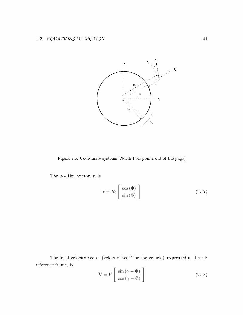
2.2. EQUATIONS OF MOTION 41
Figure 2.5: Coordinate systems (North Pole points out of the page)
The position vector, r, is
r = R0
[cos (Φ)
sin (Φ)
](2.17)
The local velocity vector (velocity �seen� be the vehicle), expressed in the EF
reference frame, is
V = V
[sin (γ − Φ)
cos (γ − Φ)
](2.18)

42 CHAPTER 2. PROBLEM FORMULATION
Then, the time derivative of the local velocity vector is
V = V
[sin (γ − Φ)
cos (γ − Φ)
]+ V γ
[cos (γ − Φ)
− sin (γ − Φ)
]+
+V Φ
[− cos (γ − Φ)
sin (γ − Φ)
](2.19)
where Φ is de�ned in Equation 2.16.
The standard relation between time derivatives of vectors in inertial and ro-
tating frames is (dr
dt
)inertial
=
(dr
dt
)rotating
+ ω × r (2.20)
In this case, ω is simply ωE. Hence, the inertial velocity, VI is
VI = V + ωE × r (2.21)
where V is the EF velocity vector observed by the vehicle (Equation 2.18).
Taking the time derivative of Equation 2.21 gives[dV
dt
]I
= V + 2ωE ×V + ωE × (ωE × r) (2.22)
since ωE is constant.
The gravitational force acting on the vehicle is given by
Fg = −mg(h)
[cos Φ
sin Φ
](2.23)

2.2. EQUATIONS OF MOTION 43
and g(h) is
g(h) =µ
(RE + h) 2 (2.24)
The inertial aerodynamic forces, drag (D) and lift (L), are given by
D = −D
[sin(γ − Φ)
cos(γ − Φ)
](2.25)
L = L
[cos(γ − Φ)
− sin(γ − Φ)
](2.26)
According to Newton's second law, ΣF = mdVI
dt. This vector equation can be
expressed as its inertial x- and y-components:
−D
msin (γ − Φ) +
L
mcos (γ − Φ)− g(h) cos Φ =
V sin (γ − Φ) + V γ cos (γ − Φ)− V Φ cos (γ − Φ)−
−2V ωE cos (γ − Φ)−R0ω2
E cos Φ (2.27)
−D
mcos (γ − Φ)− L
msin (γ − Φ)− g(h) sin Φ =
V cos (γ − Φ)− V γ sin (γ − Φ) + V Φ sin (γ − Φ) +
+2V ωE sin (γ − Φ)−R0ω2
E sin Φ (2.28)

44 CHAPTER 2. PROBLEM FORMULATION
Solving Equations 2.27 and 2.28 for V and γ gives
V = −(
µ
R 20
− ω 2E R0
)sin γ − qSrefCD(M, δs)
1
m(2.29)
γ =1
V
[−(
µ
R 20
− ω 2E R0
)cos γ + qSrefCL(M, δa, δs)
1
m
]+
V
R0
cos γ + 2ωE (2.30)
For equatorial �ight, the total pitching moment is unchanged between inertial
and local coordinate frames (see [13]). Consequently, the 3 degrees-of-freedom (3DoF)
longitudinal equations of motion are Equations 2.29 and 2.30 and
q =1
2ρV Sdref
(CM(M, δa, δs) +
dref
2VCMq(M)q
)(1
Iyy
)(2.31)
xd = V cos γRE
R0
(2.32)
h = V sin γ (2.33)
θ = q (2.34)
with auxillary equations
α = θ − γ (2.35)
M =V
a(2.36)
q =1
2ρV 2 (2.37)
R0 = RE + h (2.38)
The interested reader is directed to [13] for a complete development of the
6DoF equations of motion, as well as [14] for additional background in modeling

2.3. BALLISTIC TRAJECTORY 45
atmospheric �ight.
2.3 Ballistic Trajectory
A slender reentry vehicle with a �xed symmetric de�ection follows a ballistic tra-
jectory similar to that presented in Figures 2.6 and 2.7. The 1976 U.S. Standard
Atmosphere is modeled, and the data are obtained from MATLAB/SIMULINK sim-
ulations employing the built-in ODE15s solver.[15][16] Note the peak dynamic pres-
Figure 2.6: Velocity and dynamic pressure histories for a slender reentry vehicle on a ballistic
trajectory, δs = 10 degrees
sure occurs shortly before impact and does not correspond with peak Mach number,
but rather the sharply increasing density as the vehicle descends. Figure 2.7 demon-
strates a nearly linear �ight path angle, γ, while the angle of attack and pitch rate
oscillate rapidly until the dynamic pressure increases. This is characteristic of a lightly
damped, marginally stable system.

46 CHAPTER 2. PROBLEM FORMULATION
Figure 2.7: Flight path angle, angle of attack, and pitch rate histories for a slender reentry
vehicle on a ballistic trajectory, δs = 10 degrees
2.4 Maximum Trim Angle of Attack
At a trimmed angle of attack, all pitch rates are zero; that is,
q = 0
q = 0
From Equations 2.10 and 2.31,
αtrim = −CM0
CMα
(2.39)
However, the limits in control surface de�ections (see Figure 2.2) limit the combina-
tions of δa and δs available to trim the vehicle at a speci�ed angle of attack. Figure
2.8 presents a typical example of these limitations for a constant Mach number. The
large trim angle of attack is only available for δs between 3.8 and 5.9 degrees, while

2.4. MAXIMUM TRIM ANGLE OF ATTACK 47
reduced values of |αtrim| permit larger ranges in δs. The trim curves in Figure 2.8
intersect at the symmetric de�ection corresponding to zero static margin (neutral
static stability), where (theoretically) in�nite values of αtrim are available. However,
the linearized dynamics are not assumed to be valid for |α| > 10◦ (see Section 2.1).
Figure 2.8: Contours of constant αtrim as δa and δs vary; constant Mach number

This page intentionally left blank.

Chapter 3
Baseline Control Design
To better understand the challenges and limitations of Slender Reentry Vehicle (SRV)
control, a linear controller is designed to respond to step commands in angle of attack.
After a simpli�cation of the equations of motion, rapid development and analysis
of this controller is accomplished to identify linear controller strengths as well as
weaknesses that could be corrected with more advanced controllers.
Con�ning analysis to angle of attack tracking leads to a dual-input, single
output system. Rather than actively controlling both inputs, this chapter treats
symmetric de�ection as a parameter and discusses how symmetric de�ection can be
set based on a performance/robustness trade.
49

50 CHAPTER 3. BASELINE CONTROL DESIGN
3.1 Simpli�cation of the Equations of Motion
As presented in Section 2.2, six di�erential equations represent the longitudinal mo-
tion of the vehicle:
V = −(
µ
R 20
− ω 2e R0
)sin γ − 1
2ρV 2SCD(M, δs)
1
m(3.1)
γ =1
V
[−(
µ
R 20
− ω 2e R0
)cos γ +
1
2ρV 2SCL(M, δa, δs)
1
m
]+
V
R0
cos γ + 2ωe (3.2)
q =1
2ρV Sdref
(CM(M, δa, δs) +
dref
2VCMqq
)(1
Iyy
)(3.3)
xd = V cos γRE
R0
(3.4)
h = V sin γ (3.5)
θ = q (3.6)
The SRV has two control inputs, δs and δa; δs enters the pitch dynamics
nonlinearly (see Equation 2.13). For a constant Mach number, Equation 3.3 is ap-
proximately a second-order di�erential equation. From Equation 2.35,
α = q − γ (3.7)
While γ is certainly nonzero, it is nearly linear in time for a ballistic reentry, as
shown in Figure 2.7. Furthermore, this e�ort assumes γ does not change signi�cantly
in relation to the (faster) controller; that is, γ ≈ 0. Consequently, γ is nearly zero;
thus,
α ≈ q (3.8)
α ≈ q (3.9)

3.2. CONTROLLER DEVELOPMENT 51
Assuming the major task of the control system is to track guidance system-
generated angles of attack, the pertinent equation of motion reduces to
α =
(−[CLα0
(M) + CLαδ(M)δs
][(Xcp
l
)0(M)+
+(
Xcp
l
)δ(M)δs − Xcg
l
]l
drefα + d
2VCMq α−
− 4√M2−1
(π
180◦δa
) (Sflap
Sref
)(Xflap
l− Xcg
l
))ρV 2Sd
2Iyy
(3.10)
For a constant Mach number and altitude, Equation 3.10 is of form
α =(a1 + a2δs + a3δs
2)α + a4α + bδa (3.11)
where δs and δa are the control inputs and α and α are the states. Further inspection
shows a plant that is nonlinearly dependent on the symmetric control de�ection, δs,
with δs coupling with the angle of attack, α.
3.2 Controller Development
Treating δs as a parameter, Equation 3.11 is a linear, second-order di�erential equa-
tion of form
x = Ax + Bu (3.12)
with output y
y = Cx (3.13)
In this case, the only output is angle of attack, so C is [1 0].

52 CHAPTER 3. BASELINE CONTROL DESIGN
Since the matrix A is a function of δs, the open-loop poles of the system
vary with symmetric de�ection. Figure 3.1 shows the open-loop pole locations for
a constant Mach number and altitude. Increasing the symmetric de�ection alters
Figure 3.1: Variation in pole location with δs for a constant Mach number and altitude (not
to scale)
the system from statically unstable to statically stable. Furthermore, static stability
increases with increasing Mach numbers.[12]
Optimal control schemes for problems of this type are well-established. The
reader is directed to the large body of literature addressing optimal linear control
(e.g., [17],[18],[19]).
3.2. CONTROLLER DEVELOPMENT 53
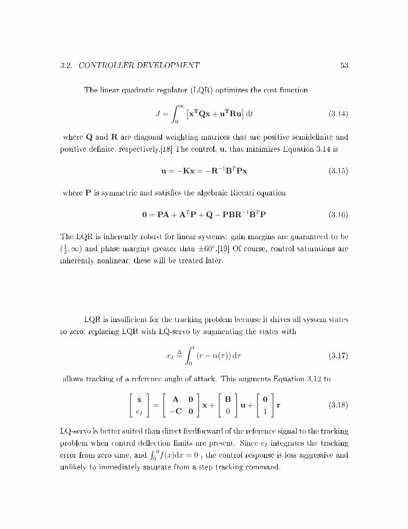
The linear quadratic regulator (LQR) optimizes the cost function
J =
∫0
∞ [xTQx + uTRu
]dt (3.14)
where Q and R are diagonal weighting matrices that are positive semide�nite and
positive de�nite, respectively.[18] The control, u, that minimizes Equation 3.14 is
u = −Kx = −R−1BTPx (3.15)
where P is symmetric and satis�es the algebraic Riccati equation
0 = PA + ATP + Q−PBR−1BTP (3.16)
The LQR is inherently robust for linear systems: gain margins are guaranteed to be
(12,∞) and phase margins greater than ±60◦.[19] Of course, control saturations are
inherently nonlinear; these will be treated later.
LQR is insu�cient for the tracking problem because it drives all system states
to zero; replacing LQR with LQ-servo by augmenting the states with
eI∆=
∫ t
0
(r − α(τ)) dτ (3.17)
allows tracking of a reference angle of attack. This augments Equation 3.12 to[x
eI
]=
[A 0
−C 0
]x +
[B
0
]u +
[0
1
]r (3.18)
LQ-servo is better suited than direct feedforward of the reference signal to the tracking
problem when control de�ection limits are present. Since eI integrates the tracking
error from zero time, and∫
0
0f(x)dx = 0 , the control response is less aggressive and
unlikely to immediately saturate from a step tracking command.

54 CHAPTER 3. BASELINE CONTROL DESIGN
Figure 3.2: Reentry pro�le
For a given �ight condition (Mach number and altitude), linear control gains
are generated for symmetric de�ections in the range [2,8] degrees. Values of δs out-
side this range give very little δa, since �ap de�ections are limited to [0,10] degrees
(see Section 2.1.1). Consequently, they are assumed to be of little use in reference
tracking. Three �ight conditions are evaluated, as shown in Table 3.1 and Figure 3.2.
Table 3.1: Flight conditions selected for analysis of the SRVMach altitude (km)3.5 06.3 205.3 50
To simplify the performance/robustness trade for variations in symmetric de-
�ection, the 10% to 90% rise time, tr, for a one degree step command is selected
as the primary indicator of tracking performance (see Figure 3.3 and the following
section).[20] A constant rise time for all symmetric de�ections sets a time domain per-
formance standard, easing the subsequent robustness analysis. Presumably, tracking

3.3. RESULTS 55
performance becomes more critical as the vehicle descends and remaining �ight time
decreases. Thus, the desired rise time decreased as the vehicle descended. At the
whole number symmetric de�ections on [2,8] degrees, the weighting matrices Q and
R are chosen such that the loop gain margin is 6 (15.6 dB) and the rise time met the
desired threshold. Q is a 3x3 matrix with nonzero terms on the main diagonal:
Q =
qα 0 0
0 qq 0
0 0 qeI
With a single control input, R is scalar; �xing R at unity left three degrees of freedom
in the search. The diagonal terms of Q are initialized according to Bryson's rule [17],
and a bisection search algorithm determined a Q such that
J = 12
(|tr − trdes
|tol · trdes
+|gm− gmdes|tol · gmdes
)< 1 (3.19)
where tol is a speci�ed tolerance. The bisection search algorithm ceased as soon as
Equation 3.19 is satis�ed.
3.3 Results
At each �ight condition, whole-number symmetric de�ections between 2 and 8 de-
grees are considered. At each symmetric de�ection, a single controller (i.e., set of
LQ-servo gains) is selected according to the development in Section 3.2. Employ-
ing MATLAB/SIMULINK and the built-in ODE15s solver[15][16], the vehicle track-
ing performance with the LQ-servo controller is simulated. Then, each controller's
performance and robustness are compared, allowing selection of an ideal symmetric
de�ection.

56 CHAPTER 3. BASELINE CONTROL DESIGN
The ensuing development follows an incremental build-up of the system:
1. The system without actuator dynamics.
2. The system with a �rst-order actuator.
3. The system with a �rst-order actuator and lead compensator.
The gains determined in Step 1 are held constant throughout the ensuing de-
velopment. This process highlights the di�culties associated with the plant itself ver-
sus those di�culties arising out of unmodeled actuator dynamics and plant/actuator
interactions.
The optimal LQ-servo gains, found using the method described in Section
3.2, are employed to track step commands from 1 to 10 degrees. Rather than com-
pare numerous time responses, three quanti�able time response characteristics are
selected:[20]
• 10% to 90% rise time, tr
• 5% settling time, ts
• magnitude of peak overshoot, mp
Figure 3.3 shows these values on a sample time response to a unity step command. The
rise time indicates how quickly the systems responds to an input command; generally,
a low time response is desirable. In this e�ort, the rise is �xed to standardize the time

3.3. RESULTS 57
Figure 3.3: Sample time response showing rise time (tr), settling time (ts), and peak over-
shoot (mp) for a unity step command
58 CHAPTER 3. BASELINE CONTROL DESIGN
responses of various con�gurations (see Section 3.2). The settling time indicates how
long it takes the response to stay �close� to the commanded value. Once again, a low
settling time is usually desirable. An in�nite settling time can be encountered if the
system approaches a limit cycle with an oscillation about the reference command. The
magnitude of the peak overshoot is the maximum di�erence between the reference
command and the time response, often expressed as percent of the reference command.
A small peak overshoot is often desirable; large peak overshoots often indicate near-
instability. However, an overdamped system exhibits zero peak overshoot; in many
cases, this is not desirable because overdamped systems can have high rise times.
Consequently, low rise time and low peak overshoot can be antagonistic. These three
time response characteristics summarize the time response in a concise, quanti�able
form.
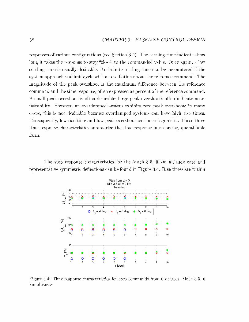
The step response characteristics for the Mach 3.5, 0 km altitude case and
representative symmetric de�ections can be found in Figure 3.4. Rise times are within
Figure 3.4: Time response characteristics for step commands from 0 degrees, Mach 3.5, 0
km altitude

3.3. RESULTS 59
10% of the speci�ed value for the 1 degree step (the design condition). Settling times
less than 250% of the desired rise time for the zero-altitude case; additionally, settling
times are lower for lower symmetric de�ections (reduced static stability). However,
the 4 degree symmetric de�ection con�guration cannot track reference commands
greater than 6 degrees; reference commands greater than 6 degrees result in controller
saturation. The vehicle is statically unstable at Mach 3.5 and 4 degrees of symmetric
de�ection; without further control authority, the system remains unstable. The peak
overshoot is consistently below 6%. The 4 degree symmetric de�ection minimized
peak overshoot for the range of commands it sucessfully tracked.
The step response characteristics for the Mach 6.3, 20 km altitude case and
representative symmetric de�ections is found in Figure 3.5. Once again, rise times
Figure 3.5: Time response characteristics for step commands from 0 degrees, Mach 6.3, 20
km altitude
are within 10% of the speci�ed value for the range of commands shown. The 6
degrees of symmetric de�ection con�guration is unable to track commands greater
than 7 degrees. Control saturation limits the tracking performance for this case.

60 CHAPTER 3. BASELINE CONTROL DESIGN
The remaining representative symmetric de�ections (4 and 5 degrees) show similar
performance across the range of reference commands shown. Peak responses are
negligible. This may motivate a faster desired rise time in later research, although
low dynamic pressure and control saturation limits may prove to be the limiting
factors.
The step response characteristics for the Mach 5.3, 50 km altitude case are
shown in Figure 3.6. The limited range of reference commands that may be tracked
Figure 3.6: Time response characteristics for step commands from 0 degrees, Mach 5.3, 50
km altitude
is immediately apparent. Symmetric de�ections outside the range shown failed to
track commands greater than 5 degrees. Rise times remain within 10% of the desired
value. Settling times increase for all cases shown as the magnitude of the reference
command increases. Likewise, peak overshoot increases from less than 5% for 1 degree
commands to well over 10% for 5 degree commands. Again, control saturation limits
the system performance.

3.3. RESULTS 61
3.3.1 Linear Gain and Phase Margins
The reference to angle of attack transfer function gain and phase margins for all three
�ight conditions are shown in Figure 3.7. These robustness margins ignore the e�ects
of control saturation. Control saturation can be a problem if the system is statically
unstable (i.e., low values of δs). A statically stable system can cope with control
saturation, although tracking performance may be diminished. Control saturation
e�ects are discussed in subsequent sections. Gain margins are all between 14.5 and
Figure 3.7: Gain and phase margins for the reference command to angle of attack loop
transfer functions as δs varies
16.5 dB, satisfying the design criteria of Section 3.2, while phase margins are greater
than 60 degrees. It is interesting to note the 13 degree rise in phase margin as δs
increases for the Mach 6.3, 20 km altitude case. Increasing symmetric de�ection
decreases phase margin 5 degrees at 0 km, and has little e�ect at 50 km.

62 CHAPTER 3. BASELINE CONTROL DESIGN
3.3.2 Initial Robustness Analysis
Although controller development assumed perfect knowledge of the plant dynamics,
the vehicle may be poorly modeled. Three uncertainties are considered. First, the
center of pressure location is likely to be known within some (possibly large) tolerance.
Second, the extreme reentry environment may cause control surface ablation, reduc-
ing control e�ectiveness. Third, asymmetric vehicle ablation may create a nonzero
pitch acceleration (moment) that modi�es the trim condition. These three e�ects are
examined below for 1 degree step commands.
The e�ects of variations in the center of pressure location and control surface
e�ectiveness are summarized in Figures 3.8, 3.9 and 3.10. Here, 0% variation in Xcp
is the nominal case; that is, there is zero variation in the center of pressure from ideal.
Conversely, 100% control e�ectiveness indicates the controls are operating with 100%
of their nominal performance. For maximum system robustness, high tolerances of
Xcp variation and low allowable control e�ectiveness are desired. The nonlinear in-
stability limit represents where the closed-loop system diverges; in practice, nonlinear
instability is de�ned to be |α| > 20◦. The center of pressure may be unknown from
unmodeled aerodynamic e�ects, vehicle ablation, poorly modeled �ight conditions,
etc.; thus, it is important to understand the bounds on center of pressure knowledge.
The allowable center of pressure variations are correlated with the linear instability
limits (i.e., when the closed-loop poles cross the jω axis). Exceptions to this occur
when the system is very statically unstable (low values of δs): then, the saturation
limits keep the control system from providing closed-loop stability. The control sat-
uration limits are where the SRV can no longer trim at the reference command (see
Section 2.4).
The control surface e�ectiveness limits are important, especially in the face
of unmodeled �ap ablation during reentry. At the 0 km altitude case, the system is

3.3. RESULTS 63
Figure 3.8: Allowable variation in center of pressure location and reduction in control e�ec-
tiveness, step command from 0 to 1 degree, Mach 3.5, 0 km altitude
Figure 3.9: Allowable variation in center of pressure location and reduced control e�ective-
ness, step command from 0 to 1 degree, Mach 6.3, 20 km altitude

64 CHAPTER 3. BASELINE CONTROL DESIGN
Figure 3.10: Allowable variation in center of pressure location and reduced control e�ective-
ness, step command from 0 to 1 degree, Mach 5.3, 50 km altitude
relatively intolerant of reduced control e�ectiveness. This intolerance is closely related
to the linear instability of the closed-loop system. Increased δs permits lower control
e�ectiveness before reaching instability. Higher Mach numbers may remain stable
for decreased values of control e�ectiveness, but these high Mach numbers occur at
higher altitudes during the reentry. Consequently, dynamic pressures are reduced and
overall control e�ectiveness is likewise reduced. Thus, control saturation limits are
reached sooner in the face of reduced control e�ectiveness, even though these may
not be destabilizing. This is apparent in the cases at 20 and 50 km altitude: for large
symmetric de�ections (greater static stability), the control saturation limit is reached
before the trajectories diverge.
The in�uence of an external pitch acceleration (speci�c moment) is evaluated
and shown in Figures 3.11, 3.12, and 3.13. This is considered because asymmetric
ablation may cause an external pitching moment on the vehicle. At high dynamic
pressures, the controls are more e�ective at reducing an external moment, while

3.3. RESULTS 65
lower dynamic pressures reduce control e�ectiveness. In the presence of tight control
de�ection limits, even a small external acceleration (on the order of 15 deg/s2) can
cause control saturation and instability. The case at 20 km (Figure 3.12) is especially
Figure 3.11: Robustness to external pitch acceleration, step command from 0 to 1 degree,
Mach 3.5, 0 km altitude
interesting. The other two cases are fairly constant across the range of δs, but the
intermediate altitude shows a minimum performance for symmetric de�ections near 3
and 4 degrees. Robustness to external pitch accelerations is gained when symmetric
de�ections are decreased to 2 degrees or increased to 8 degrees.
Robustness for reference commands greater than 1 degree is also considered.
Plots similar to Figures 3.8�3.13 for step commands from 0 to 10 degrees can be
found in Appendix A; they are omitted here for the sake of brevity. The robustness
of larger step commands will be revisited in subsequent sections of this chapter.
Thus far, the robustness analysis highlighted three separate behaviors. First,
static instability coupled with poor plant knowledge (center of pressure variation,

66 CHAPTER 3. BASELINE CONTROL DESIGN
Figure 3.12: Robustness to external pitch acceleration, step command from 0 to 1 degree,
Mach 6.3, 20 km altitude
Figure 3.13: Robustness to external pitch acceleration, step command from 0 to 1 degree,
Mach 5.3, 50 km altitude
3.3. RESULTS 67
reduced control e�ectiveness, external pitching moment) can lead to control surface
saturation, e�ectively eliminating the active control. Thus, the system becomes un-
stable. Second, if the control saturates but the vehicle is statically stable, the distur-
bance does not destabilize the system; however, the o�-nominal plant cannot track
reference commands. Finally, su�cient control authority can exist to compensate for
the plant disturbance. Then, the vehicle becomes unstable when the linear robustness
bounds reach zero and the closed-loop poles cross the jω axis.
As might be expected, larger reference commands require better plant knowl-
edge to maintain su�cient tracking and closed-loop stability. Furthermore, greater
total control e�ectiveness (i.e., higher dynamic pressures) are more tolerant of o�-
nominal plants.
3.3.3 Actuator Dynamics
The addition of a �rst-order actuator of the form ps+p
decreased the performance of the
system, especially at lower altitudes where the short period dynamics are signi�cantly
faster. Figure 3.14 demonstrates the loss of gain and phase margin for the Mach 3.5,
0 km altitude case (compare to Figure 3.7). The margins at 20 and 50 km are largely
unchanged because the plant dynamics are signi�cantly slower than the actuator
dynamics.
The vehicle time response characteristics at Mach 3.5, 0 km altitude are sum-
marized in Figure 3.15. Similar graphs for the additional two �ight conditions studied
are shown in Appendix A. These are omitted here because performance does not
change signi�cantly for these cases.
68 CHAPTER 3. BASELINE CONTROL DESIGN
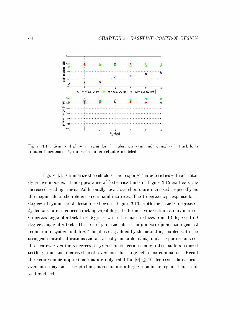
Figure 3.14: Gain and phase margins for the reference command to angle of attack loop
transfer functions as δs varies, 1st order actuator modeled
Figure 3.15 summarize the vehicle's time response characteristics with actuator
dynamics modeled. The appearance of faster rise times in Figure 3.15 contrasts the
increased settling times. Additionally, peak overshoots are increased, especially as
the magnitude of the reference command increases. The 1 degree step response for 4
degrees of symmetric de�ection is shown in Figure 3.16. Both the 4 and 6 degrees of
δs demonstrate a reduced tracking capability; the former reduces from a maximum of
6 degrees angle of attack to 4 degrees, while the latter reduces from 10 degrees to 9
degrees angle of attack. The loss of gain and phase margin corresponds to a general
reduction in system stability. The phase lag added by the actuator, coupled with the
stringent control saturations and a statically unstable plant, limit the performance of
these cases. Even the 8 degrees of symmetric de�ection con�guration su�ers reduced
settling time and increased peak overshoot for large reference commands. Recall
the aerodynamic approximations are only valid for |α| ≤ 10 degrees; a large peak
overshoot may push the pitching moment into a highly nonlinear region that is not
well-modeled.

3.3. RESULTS 69
Figure 3.15: Time response characteristics for step commands from 0 degrees, Mach 3.5, 0
km altitude, 1st order actuator modeled
Figure 3.16: 1 degree step response with actuator, Mach 3.5, 0 km altitude

70 CHAPTER 3. BASELINE CONTROL DESIGN
Figure 3.17 reveals the robustness to center of pressure variation is reduced for
all cases to approximately 10% (compare to Figure 3.8). The robustness to external
Figure 3.17: Allowable variation in center of pressure location and reduced control e�ec-
tiveness, step command from 0 to 1 degree, Mach 3.5, 0 km altitude, 1st order actuator
modeled
pitch accelerations is also reduced, as shown in Figure 3.18.
As previously mentioned, the actuator dynamics did not signi�cantly a�ect
the Mach 6.3, 20 km case or the Mach 5.3, 50 km case. The robustness summaries of
these cases with the actuator dynamics included are shown in Appendix A
3.3.4 Addition of Lead Compensator
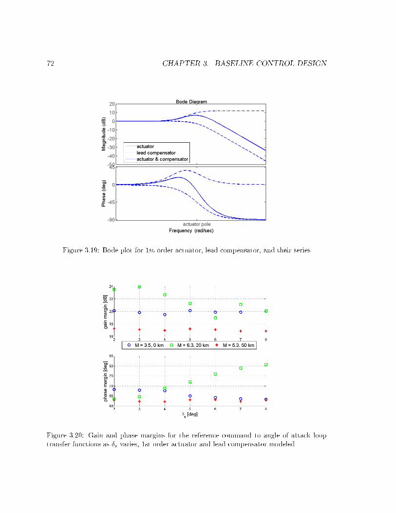
To eliminate the oscillatory e�ect of actuator dynamics on vehicle tracking perfor-
mance, a lead compensator of the form s+as+b
, a < b, is added. A simple pole-zero can-
3.3. RESULTS 71
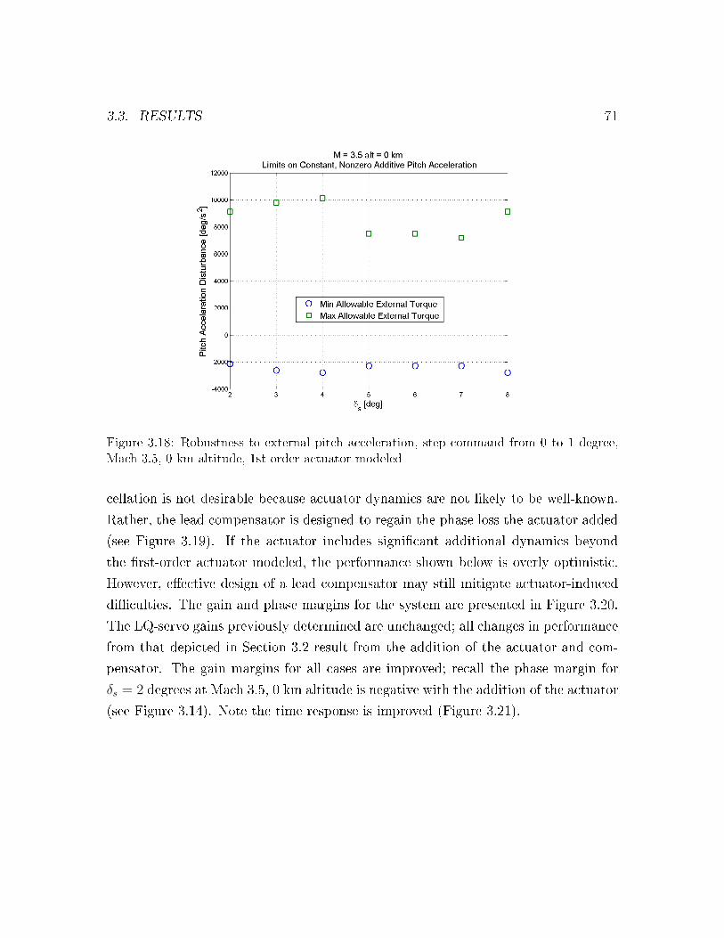
Figure 3.18: Robustness to external pitch acceleration, step command from 0 to 1 degree,
Mach 3.5, 0 km altitude, 1st order actuator modeled
cellation is not desirable because actuator dynamics are not likely to be well-known.
Rather, the lead compensator is designed to regain the phase loss the actuator added
(see Figure 3.19). If the actuator includes signi�cant additional dynamics beyond
the �rst-order actuator modeled, the performance shown below is overly optimistic.
However, e�ective design of a lead compensator may still mitigate actuator-induced
di�culties. The gain and phase margins for the system are presented in Figure 3.20.
The LQ-servo gains previously determined are unchanged; all changes in performance
from that depicted in Section 3.2 result from the addition of the actuator and com-
pensator. The gain margins for all cases are improved; recall the phase margin for
δs = 2 degrees at Mach 3.5, 0 km altitude is negative with the addition of the actuator
(see Figure 3.14). Note the time response is improved (Figure 3.21).
72 CHAPTER 3. BASELINE CONTROL DESIGN
Figure 3.19: Bode plot for 1st order actuator, lead compensator, and their series
Figure 3.20: Gain and phase margins for the reference command to angle of attack loop
transfer functions as δs varies, 1st order actuator and lead compensator modeled

3.3. RESULTS 73
Figure 3.21: 1 degree step response, Mach 3.5, 0 km altitude, 1st order actuator and lead
compensator
3.3.5 LQ-servo Performance at M = 3.5, 0 km Altitude
The time response summary for Mach 3.5, 0 km altitude with the actuator and lead
compensator is presented in Figure 3.22. The rise times are increased for all cases
shown, although the settling times are improved. The settling times for small reference
commands and 8 degrees of symmetric de�ection are improved approximately 50%.
Peak overshoots are less than 8%, compared to over 20% for the actuator alone.
Additionally, 4 degrees of symmetric de�ection still cannot track reference commands
greater than 6 degrees.
Compare the robustness to center of pressure location and control e�ectiveness
for 1 and 10 degree step commands (Figures 3.23 and 3.24). The smaller reference
command is limited by the linear instability limit, while the larger reference command

74 CHAPTER 3. BASELINE CONTROL DESIGN
Figure 3.22: Time response characteristics for step commands from 0 degrees, Mach 3.5, 0
km altitude, actuator and lead compensator modeled
3.3. RESULTS 75
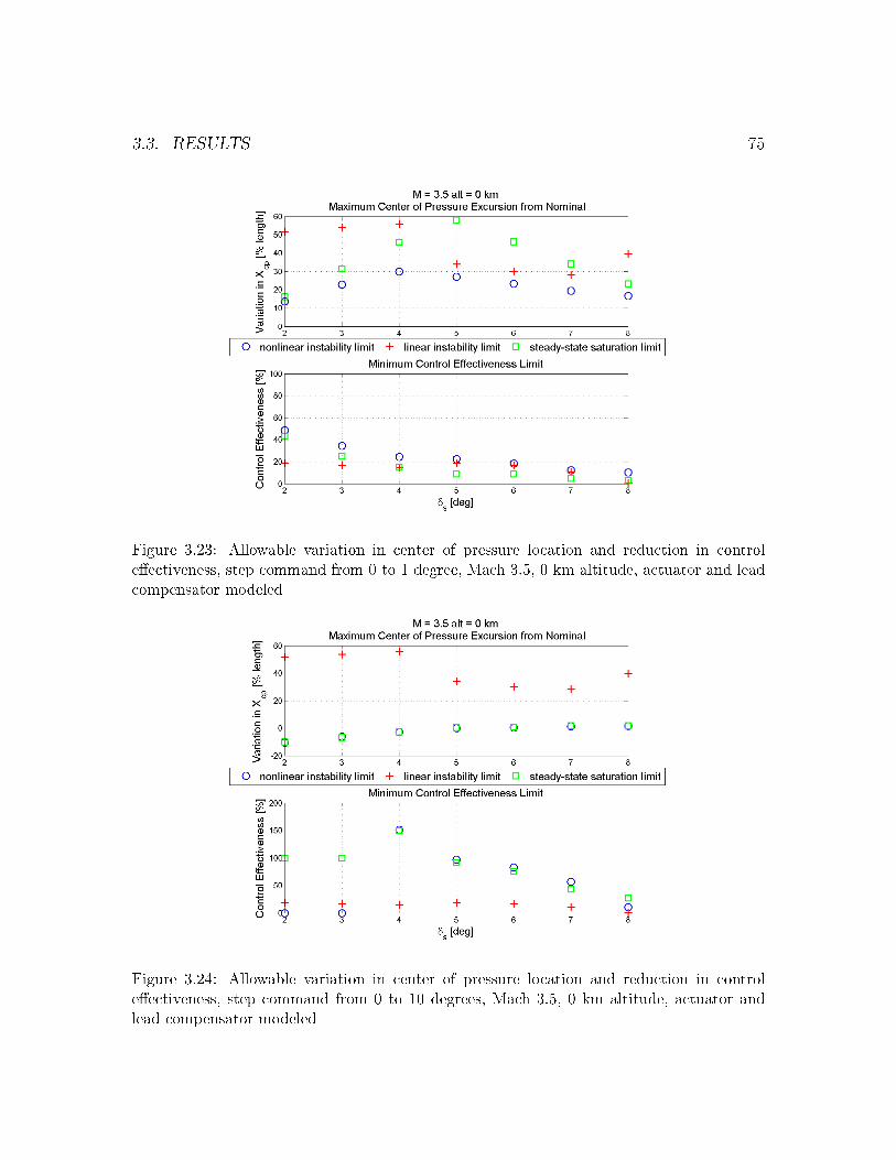
Figure 3.23: Allowable variation in center of pressure location and reduction in control
e�ectiveness, step command from 0 to 1 degree, Mach 3.5, 0 km altitude, actuator and lead
compensator modeled
Figure 3.24: Allowable variation in center of pressure location and reduction in control
e�ectiveness, step command from 0 to 10 degrees, Mach 3.5, 0 km altitude, actuator and
lead compensator modeled

76 CHAPTER 3. BASELINE CONTROL DESIGN
has its robustness limits tied to controller saturation. Note symmetric de�ections un-
der 5 degrees are unstable for a 10 degree command. This is apparent since the
allowable variation in Xcp is negative, indicating the nominal case (zero variation) is
unstable. Additionally, these symmetric de�ections require more than 100% of avail-
able control authority. Consequently, the �aps saturate and are unable to stabilize
(or control) the system for δs less than 5 degrees.
Figures 3.22 show a decrease in rise time and an improvement in robustness
to static margin uncertainty and reduced controller e�ectiveness, compared to the
baseline case (Figure 3.4). However, this is misleading: the actuator is modeled as an
ideal, 1st order exponential rise. In fact, the actuator may have additional dynamics,
and these dynamics may be poorly modeled or unknown. While it is unreasonable to
assume the lead compensator can totally eliminate all undesired actuator e�ects, it
can be e�ective at reducing the severity of these e�ects.
The robustness to external pitch accelerations for 1 and 10 degree step com-
mands are shown in Figures 3.25 and 3.26.
As might be expected, the controller is more capable of tracking a smaller
reference command in the face of an external pitching moment. Recall symmetric
de�ections under 5 degrees are unstable in tracking the 10 degree reference command.

3.3. RESULTS 77
Figure 3.25: Robustness to external pitch acceleration, step command from 0 to 1 degree,
Mach 3.5, 0 km altitude, actuator and lead compensator modeled
Figure 3.26: Robustness to external pitch acceleration, step command from 0 to 10 degrees,
Mach 3.5, 0 km altitude, actuator and lead compensator modeled

78 CHAPTER 3. BASELINE CONTROL DESIGN
3.3.6 LQ-servo Performance at M = 6.3, 20 km Altitude
The time response summary for Mach 6.3, 20 km altitude is presented in Figure 3.27.
The 6 degree δs con�guration is unstable for commands greater than 7 degrees, and
Figure 3.27: Time response characteristics for step commands from 0 degrees, Mach 6.3, 20
km altitude, actuator and lead compensator modeled
the large settling time at 7 degrees indicate this case is highly oscillatory. The cases
for 4 and 5 degrees of symmetric de�ection show little variation in rise time, settling
time, or peak overshoot for the range of step commands presented. Peak overshoots
are minimal.
The robustness to center of pressure variation and control e�ectiveness for 1
and 10 degree steps is shown in Figure 3.28 and 3.29. From a stability point of
view, symmetric de�ections of 7 and 8 degrees provide the greatest robustness to

3.3. RESULTS 79
Figure 3.28: Allowable variation in center of pressure location and reduction in control
e�ectiveness, step command from 0 to 1 degree, Mach 6.3, 20 km altitude, actuator and lead
compensator modeled
Figure 3.29: Allowable variation in center of pressure location and reduction in control
e�ectiveness, step command from 0 to 10 degrees, Mach 6.3, 20 km altitude, actuator and
lead compensator modeled
80 CHAPTER 3. BASELINE CONTROL DESIGN
variation in static margin when reference commands are small. However, Figure 3.28
also demonstrates that a reduction in control surface e�ectiveness (i.e., control surface
ablation) for δs greater than 5 degrees can result in control surface saturation before
instability is reached, even for a 1 degree reference command. In such a con�guration,
the vehicle would remain stable but unable to track the reference command.
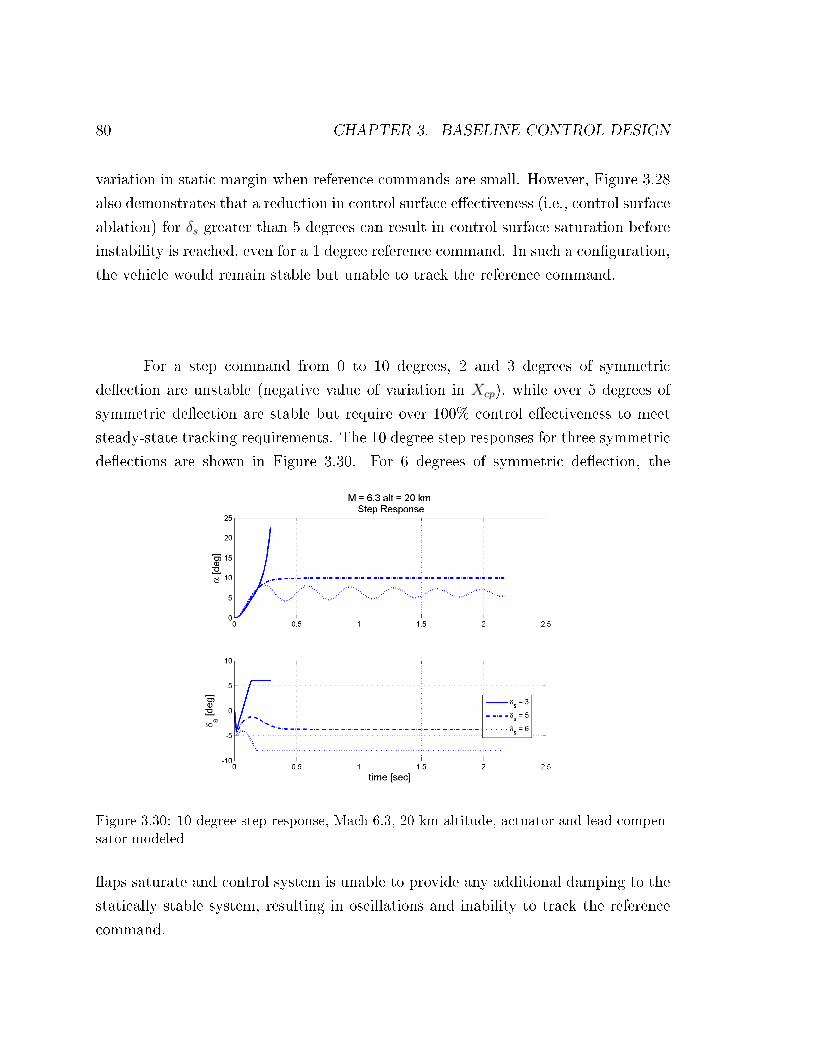
For a step command from 0 to 10 degrees, 2 and 3 degrees of symmetric
de�ection are unstable (negative value of variation in Xcp), while over 5 degrees of
symmetric de�ection are stable but require over 100% control e�ectiveness to meet
steady-state tracking requirements. The 10 degree step responses for three symmetric
de�ections are shown in Figure 3.30. For 6 degrees of symmetric de�ection, the
Figure 3.30: 10 degree step response, Mach 6.3, 20 km altitude, actuator and lead compen-
sator modeled
�aps saturate and control system is unable to provide any additional damping to the
statically stable system, resulting in oscillations and inability to track the reference
command.
3.3. RESULTS 81
The vehicle's robustness to external pitch accelerations for both 1 and 10
degree step commands is summarized in Figure 3.31 and 3.32. For the 1 degree step,
a minimum pitch acceleration rejection band is still present between 3 and 4 degrees
of symmetric de�ection. For a 10 degree step, symmetric de�ections greater 5 degrees
provide similar levels of external pitching moment rejection.
In the face of plant uncertainty, small reference commands may be better suited
to symmetric de�ections of 7�8 degrees, while large reference commands clearly favor
5 degrees of symmetric de�ection.

82 CHAPTER 3. BASELINE CONTROL DESIGN
Figure 3.31: Robustness to external pitch acceleration, step command from 0 to 1 degrees,
Mach 6.3, 20 km altitude, actuator and lead compensator modeled
Figure 3.32: Robustness to external pitch acceleration, step command from 0 to 10 degrees,
Mach 6.3, 20 km altitude, actuator and lead compensator modeled
3.3. RESULTS 83
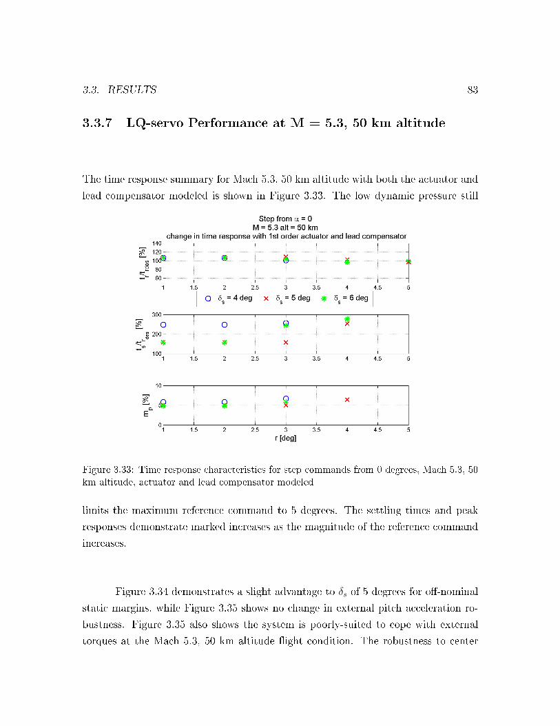
3.3.7 LQ-servo Performance at M = 5.3, 50 km altitude
The time response summary for Mach 5.3, 50 km altitude with both the actuator and
lead compensator modeled is shown in Figure 3.33. The low dynamic pressure still
Figure 3.33: Time response characteristics for step commands from 0 degrees, Mach 5.3, 50
km altitude, actuator and lead compensator modeled
limits the maximum reference command to 5 degrees. The settling times and peak
responses demonstrate marked increases as the magnitude of the reference command
increases.
Figure 3.34 demonstrates a slight advantage to δs of 5 degrees for o�-nominal
static margins, while Figure 3.35 shows no change in external pitch acceleration ro-
bustness. Figure 3.35 also shows the system is poorly-suited to cope with external
torques at the Mach 5.3, 50 km altitude �ight condition. The robustness to center
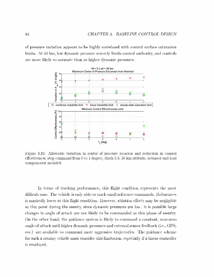
84 CHAPTER 3. BASELINE CONTROL DESIGN
of pressure variation appears to be highly correlated with control surface saturation
limits. At 50 km, low dynamic pressure severely limits control authority, and controls
are more likely to saturate than at higher dynamic pressures.
Figure 3.34: Allowable variation in center of pressure location and reduction in control
e�ectiveness, step command from 0 to 1 degree, Mach 5.3, 50 km altitude, actuator and lead
compensator modeled
In terms of tracking performance, this �ight condition represents the most
di�cult case. The vehicle is only able to track small reference commands. Robustness
is markedly lower at this �ight condition. However, ablation e�ects may be negligible
at this point during the reentry since dynamic pressures are low. It is possible large
changes in angle of attack are not likely to be commanded at this phase of reentry.
On the other hand, the guidance system is likely to command a constant, near-zero
angle of attack until higher dynamic pressures and external sensor feedback (i.e., GPS,
etc.) are available to command more aggressive trajectories. The guidance scheme
for such a reentry vehicle must consider this limitation, especially if a linear controller
is employed.

3.4. LINEAR CONTROL CONCLUSIONS 85
Figure 3.35: Robustness to external pitch acceleration, step command from 0 to 1 degree,
Mach 5.3, 50 km altitude, actuator and lead compensator modeled
3.4 Linear Control Conclusions
The linear controller tracked small commanded angles of attack well when the vehicle
aerodynamics are well known. The addition of a 1st order actuator reduced perfor-
mance when vehicle dynamics are fast (e.g., at 0 km altitude), but a lead compensator
demonstrated its ability to recover much of the actuator-induced phase lag. The con-
troller handled some degree of control e�ectiveness reduction. However, variations
in static margin, either from poorly-modeled center of pressure or movement in the
center of gravity from ablation, limited the e�ectiveness of the LQ-servo controller.
Much of the LQ-servo robust performance di�culties arose from saturation in the
control surface de�ections�this nonlinearity is hard to overcome with a linear SISO
system. The control saturations are reached when larger angles of attack are com-
manded, especially at low dynamic pressures. The remainder of this e�ort sought to
improve the performance over the LQ-servo controller.

86 CHAPTER 3. BASELINE CONTROL DESIGN
At this point, the linear controller for each Mach/altitude combination is �xed
to provide a �baseline� to evaluate other controllers. At each �ight condition, Table
3.2 shows the selected symmetric de�ection: While somewhat arbitrary, an emphasis
Table 3.2: Selected δs for each �ight conditionMach altitude (km) δs [deg]3.5 0 86.3 20 55.3 50 5
is placed on time response and robustness to static margin uncertainty (allowable
variation in Xcp). In any case, an �optimal� value of symmetric de�ection for the
LQ-servo controller can be further investigated in the future, possibly improving the
performance of the control schemes presented later in this e�ort.
Chapter 4
Hybrid Switching-Linear Controller
The baseline Linear Quadratic Servo (LQ-servo) controller presented in Chapter 3
performed well for small step commands in the presence of perfect plant uncertainty.
However, control saturation limits presented nonlinearities that limited tracking per-
formance or introduced instabilities to the system. In an e�ort to exploit the perfor-
mance of the LQ-servo controller but gain robust performance, a multi-mode, hybrid
switching-linear controller (SLC) is developed.
4.1 Motivation
The di�culty of the linear controller commanding large steps in α lies in switching
from one saturated command to the other. Many of the trajectories greatly exceed
87

88 CHAPTER 4. HYBRID SWITCHING-LINEAR CONTROLLER
10 degrees angle of attack. In Section 2.1, the aerodynamic model was only assumed
valid for |α| ≤ 10 degrees. Consequently, these large overshoots may pose a signi�cant
problem. Consider the phase plane for a 10 degree angle of attack reference command
(Figure 4.1). The trajectory that begins at 5 degrees angle of attack is of particular
Figure 4.1: Phase plane for 10 degree reference command, M = 3.5, 0 km altitude, δs = 8
degrees
interest. The initial behavior is in the �wrong direction�; that is, the initial behavior
of the vehicle is to begin a negative pitch rate, even though a positive pitch rate
is clearly desirable to increase the angle of attack to 10 degrees. Additionally, the
control switches between saturation limits twice before remaining within the control
de�ection bounds (see Figure 4.2). As a result, the peak overshoot is signi�cant, as
is control activity. This �wrong direction� behavior results from the tracking error
integral, eI , being initialized to zero. It must �wind up� enough to trim the vehicle
at 10 degrees. The zero initial condition is su�cient when the initial angle of attack
is likewise zero, but nonzero initial angles of attack must initialize eI at a nonzero
value. The LQ-servo controller previously developed does not have a mechanism to
accomplish this.

4.1. MOTIVATION 89
Figure 4.2: Step response from 5 to 10 degrees, M = 3.5, 0 km altitude, δs = 8 degrees
The SLC developed has two distinct modes. The �rst mode is completely
saturated control at either the positive or negative limit of δa. Switching between
these two is based on a switching curve in the phase plane. The second mode is the
LQ-servo controller previously developed, with the switch occurring along another
curve in the phase plane. The qualitative control strategy is to drive the phase plane
trajectory as rapidly as possible into the LQ-servo control region, which causes the
system to converge to the reference command. The advantage of this approach is that
small commands take advantage of the linear controller's performance and robustness,
while larger commands bypass the linear controller when it would be saturated and
possibly near instability or a limit cycle.

90 CHAPTER 4. HYBRID SWITCHING-LINEAR CONTROLLER
4.2 Phase Plane Analysis
For each �ight condition with the linear controller in place, the phase plane of initial
conditions can be subdivided into three stable regions. The �rst region is stable with
satisfactory tracking performance but possibly saturated controls during the transient
response. Here, �satisfactory� tracking performance is de�ned by two criteria:
• rise time (10% to 90% of commanded value) meets speci�cation, within 5%
• settling time (between 95% and 105% of commanded value) less than 4 rise
times
The second region is stable, but does not meet the tracking parameters speci�ed
above. The third region is denoted by totally unsaturated controls. This last region
represents a completely linear system; as such, the inherent LQR stability margins
apply (see Section 3.1). Admittedly, this �nal region is very small in relation to
the other regions, often appearing as a line segment. The 5 and 10 degree reference
commands at Mach 5.3, 50 km altitude do not show regions of unsaturated control.
These three regions can be seen in Figures 4.3-4.5. Unstable initial conditions
are those points without any marker.
A controller can exploit the unsaturated control conditions if all trajectories
could be controlled to this region. It is interesting to note the unsaturated region does
not necessarily correspond with the commanded angle of attack, especially with large
reference commands. Recall, the states α and q were augmented with the integral

4.2. PHASE PLANE ANALYSIS 91
Figure 4.3: Phase plane of stable initial conditions, LQ-servo, M = 3.5, 0 km altitude, δs =
8 degrees
Figure 4.4: Phase plane of stable initial conditions, LQ-servo, M = 6.3, 20 km altitude, δs
= 5 degrees
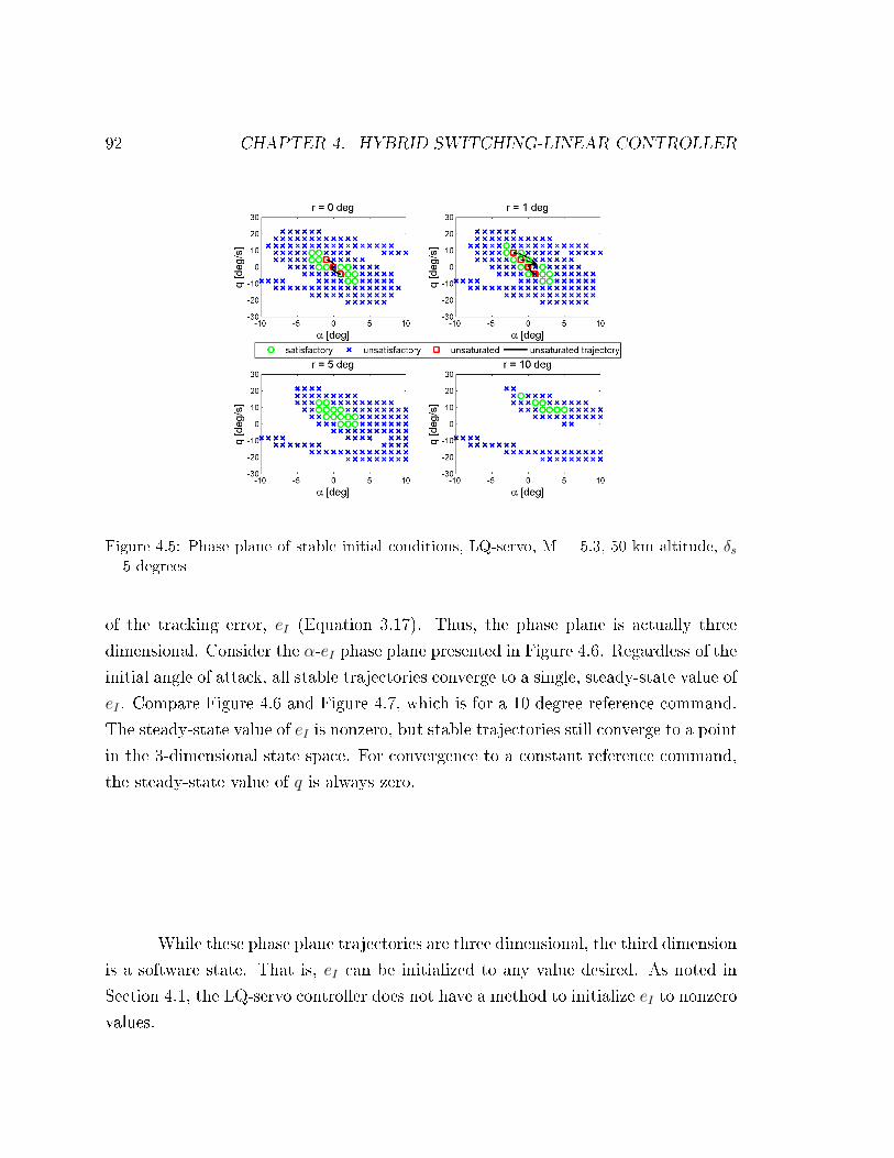
92 CHAPTER 4. HYBRID SWITCHING-LINEAR CONTROLLER
Figure 4.5: Phase plane of stable initial conditions, LQ-servo, M = 5.3, 50 km altitude, δs
= 5 degrees
of the tracking error, eI (Equation 3.17). Thus, the phase plane is actually three
dimensional. Consider the α-eI phase plane presented in Figure 4.6. Regardless of the
initial angle of attack, all stable trajectories converge to a single, steady-state value of
eI . Compare Figure 4.6 and Figure 4.7, which is for a 10 degree reference command.
The steady-state value of eI is nonzero, but stable trajectories still converge to a point
in the 3-dimensional state space. For convergence to a constant reference command,
the steady-state value of q is always zero.
While these phase plane trajectories are three dimensional, the third dimension
is a software state. That is, eI can be initialized to any value desired. As noted in
Section 4.1, the LQ-servo controller does not have a method to initialize eI to nonzero
values.

4.2. PHASE PLANE ANALYSIS 93
Figure 4.6: Zero pitch rate phase plane, eI vs α for a 0 degree reference command, M = 3.5,
0 km altitude, δs = 8 degrees
Figure 4.7: Zero pitch rate phase plane, eI vs α for a 10 degree reference command, M =
3.5, 0 km altitude, δs = 8 degrees

94 CHAPTER 4. HYBRID SWITCHING-LINEAR CONTROLLER
4.3 Switching Control Design
To improve upon the LQ-servo's performance in tracking large step commands, a
Switching Linear Controller (SLC) was developed. The SLC employed one of two
control strategies. The �rst strategy employed a saturated nonlinear controller. Its
purpose is to rapidly position the system to a state where the linear controller performs
well. The second control strategy was the previously-developed LQ-servo controller,
with an appropriate initialization of the state eI .
Observing Figures 4.3, 4.4, and 4.5, a negative trend is apparent through
the unsaturated control region of initial conditions. If the phase plane trajectory
reaches these points, it converges without control saturation to the reference condition.
Decreasing initial values of α indicate increased initial values in initial q and vice versa.
For example, Figure 4.3, r = 0, shows a narrow region of unsaturated controls that
intersects the points (-3◦,250◦/s), (0◦,0◦/s), and (3◦,-250◦/s). Similarly, the additional
�ight conditions and reference commands demonstrate regions where increasing α
strictly decreases q. A linear approximation of this trend gives
q∗ = m∗(α− r) (4.1)
where m∗ is the slope of the switching line. Given a state [α q], the value of q∗
can be calculated. If q > q∗, the control should be δamax , while q < q∗ indicates the
control should be −δamax . The purpose of this control is to drive the trajectory to
the linear region as quickly as possible. This is similar to the classic minimum-time
problem in constrained optimal control (e.g., [18]).
The centroid of the unsaturated control region (arithmetic mean of all points
within this region) varies with the value of the reference command. Let the centroid

4.3. SWITCHING CONTROL DESIGN 95
o�set from the origin, [αc qc]T , be[αc
qc
]=
[∆α
∆q
]r (4.2)
Since this centroid is within the unsaturated control region of initial conditions,
initializing eI to zero results in a satisfactory time response.
At this point, it may be reasonable to expect another curve de�nes the reset
of the error integral, eI . That is, the q∗ curve de�nes the switch between saturated
controllers, while a separate curve de�nes the initialization of the LQ-servo controller
state eI (integrated tracking error). De�ning this integral reset curve as the line that
passes through [αc qc]T and [r 0]T (the reference command) gives
qs =∆q
∆α − 1(α− r) (4.3)
While the saturated nonlinear controller is active, the state eI is irrelevant. However,
eI must be properly initialized upon intersection with the qs curve. To accomplish
this, assume the steady-state value of the error integral, designated eIf, is a linear
function of the reference command:
eIf= εr (4.4)
Note Equation 4.4 is nonzero only for nonzero values of reference commands, which
agrees with Figures 4.6 and 4.7.
Now, eI0 must be parameterized along the reset line, qs. At the reference
condition, eI0 = eIf= εr. At the point [αc qc]T (unsaturated region centroid),
eI0 = 0. The initialization of the error integral, eI0 , is then
eI0 =ε
1−∆α
(α−∆αr) (4.5)

96 CHAPTER 4. HYBRID SWITCHING-LINEAR CONTROLLER
Upon implementation, trajectories are controlled by the saturated control until
the phase plane trajectory intersects the qs curve (Equation 4.3). At this point, the
error integral state, eI , is initialized to the value determined by Equation 4.5; the
linear controller then controls the trajectory to the reference command. In practice,
the initial nonlinear control is resumed each time the reference trajectory changes:
∂r
∂t6= 0
This reset limits the guidance commands to constant angles of attack (step com-
mands), and the frequency of these steps must be su�ciently low so steady-state
tracking can be achieved. However, the controller reset method can be altered in the
future to match the implemented guidance scheme.
A challenge of switching controllers occurs when the control input �chatters�
along the switching boundary, oscillating between the minimum and maximum de-
�ections. Presumably, this control chattering could continue without the control
architecture switching to the linear controller, as in Figure 4.8. This chattering can
be remedied by setting the switching curve slope, m∗ (see Equation 4.1), to the slope
of the qs curve (Equation 4.3). E�ectively, this prevents the control from switching
between saturated de�ections by de�ning one switching curve. One initially saturated
input controls the phase plane trajectories, followed by a switch (along the common
q∗-qs switching curve) to the linear controller with proper initialization of eI .
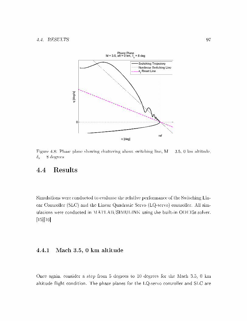
4.4. RESULTS 97
Figure 4.8: Phase plane showing chattering about switching line, M = 3.5, 0 km altitude,
δs = 8 degrees
4.4 Results
Simulations were conducted to evaluate the relative performance of the Switching Lin-
ear Controller (SLC) and the Linear Quadratic Servo (LQ-servo) controller. All sim-
ulations were conducted in MATLAB/SIMULINK using the built-in ODE15s solver.
[15][16]
4.4.1 Mach 3.5, 0 km altitude
Once again, consider a step from 5 degrees to 10 degrees for the Mach 3.5, 0 km
altitude �ight condition. The phase planes for the LQ-servo controller and SLC are

98 CHAPTER 4. HYBRID SWITCHING-LINEAR CONTROLLER
Figure 4.9: Phase plane, SLC and LQ-servo, Mach 3.5, 0 km altitude, δs = 8 degrees
presented in Figure 4.9. The initial negative pitch rate is eliminated, as is a signi�cant
portion of the overshoot. The time responses are compared in Figure 4.10. Since the
linear controller initializes eI to 0, this integral must �wind up� enough to maintain
a nonzero angle of attack. When the commanded angle of attack is greater than this
initial angle of attack, the linear controller will tend to return to 0 degrees angle of
attack until eI reaches a su�cient value to overcome this negative pitch rate. The
SLC eliminates this �wind up� by directly initializing eI to an appropriate value. As
expected, δa saturates until the phase plane trajectory intersects the eI reset curve,
when the LQ-servo controller is activated. Control activity is reduced over the linear
controller, as is the peak overshoot and settling time.
Consider the especially di�cult case of a step from -10 degrees to 10 de-
grees, presented in Figure 4.11. The magnitude of the peak overshoot is reduced
approximately 90%, resulting in a much more favorable time response for the SLC.
Furthermore, the peak overshoot extends very little into angle of attacks greater than
10 degrees, where the aerodynamic model may break down.

4.4. RESULTS 99
Figure 4.10: Time response to a step command from 5 to 10 degrees, SLC and LQ-servo,
Mach 3.5, 0 km altitude, δs = 8 degrees
Figure 4.11: Time response to a step command from -10 to 10 degrees, SLC and LQ-servo,
Mach 3.5, 0 km altitude, δs = 8 degrees

100 CHAPTER 4. HYBRID SWITCHING-LINEAR CONTROLLER
Although the switching controller improved the time response characteristics
over the LQ-servo controller, it did not provide signi�cant robustness bene�ts at
Mach 3.5 and 0 km altitude. Since the SLC incorporated the previously developed
LQ-servo control scheme, the LQ-servo robustness bounds a�ect the SLC robustness
bounds. Figure 4.12 summarizes the stability limits of center of pressure uncertainty
and reduced control surface e�ectiveness.
Figure 4.12: Robustness comparison of the SLC and LQ-servo from α = 0 deg for various
reference commands, Mach 3.5, 0 km altitude, δs = 8 degrees
A summary of the improvement in rise time, settling time, and peak overshoot
is presented in Figure 4.13. Rise times increased slightly, but settling times were
reduced to 60 percent of the LQ-servo settling time. The SLC also provided a slight
reduction in peak overshoot.

4.4. RESULTS 101
Figure 4.13: Time response characteristics for the SLC as a percent of the LQ-servo Char-
acteristics for various step commands from 0 degrees, Mach 3.5, 0 km altitude, δs = 8
degrees
4.4.2 Mach 6.3, 20 km altitude
For 5 degrees of symmetric de�ection, a step command from 0 to 10 degrees was
tracked well by the LQ-servo controller (see Figure 3.30). The SLC matched this
performance well (Figures 4.14 and 4.15), but improved on the performance of a step
from 5 to 10 degrees (Figures 4.16 and 4.17). This highlights the elimination in the
�wind up� period describes in Section 4.4.1.

102 CHAPTER 4. HYBRID SWITCHING-LINEAR CONTROLLER
Figure 4.14: Phase plane, step command from 0 to 10 degrees, SLC and LQ-servo, M = 6.3,
20 km altitude, δs = 5 degrees
Figure 4.15: Time response to a step command from 0 to 10 degrees, SLC and LQ-servo,
Mach 6.3, 20 km altitude, δs = 5 degrees
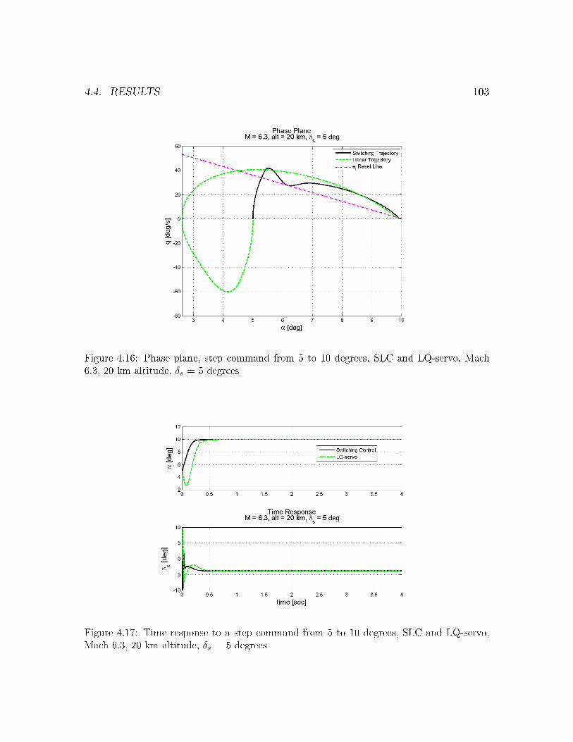
4.4. RESULTS 103
Figure 4.16: Phase plane, step command from 5 to 10 degrees, SLC and LQ-servo, Mach
6.3, 20 km altitude, δs = 5 degrees
Figure 4.17: Time response to a step command from 5 to 10 degrees, SLC and LQ-servo,
Mach 6.3, 20 km altitude, δs = 5 degrees

104 CHAPTER 4. HYBRID SWITCHING-LINEAR CONTROLLER
When commanding a step from -10 to 10 degrees, the LQ-servo's overshoot is
eliminated with the SRC (Figures 4.18 and 4.19).
Figure 4.18: Phase plane, step command from -10 to 10 degrees, SLC and LQ-servo, Mach
6.3, 20 km altitude, δs = 5 degrees
The SLC did not provide any additional robustness over the LQ-servo con-
troller; a summary of the allowable center of pressure excursion and control e�ective-
ness reduction is shown in Figure 4.20
A summary of the improvement in rise time, settling time, and peak overshoot
is presented in Figure 4.21. Except for the 1 degree step, the rise times and settling
times were reduced up to 15 and 30 percent, respectively. Peak responses were almost
unchanged.
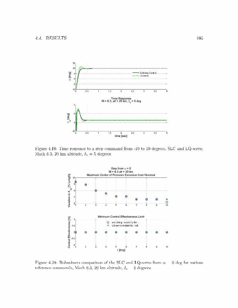
4.4. RESULTS 105
Figure 4.19: Time response to a step command from -10 to 10 degrees, SLC and LQ-servo,
Mach 6.3, 20 km altitude, δs = 5 degrees
Figure 4.20: Robustness comparison of the SLC and LQ-servo from α = 0 deg for various
reference commands, Mach 6.3, 20 km altitude, δs = 5 degrees

106 CHAPTER 4. HYBRID SWITCHING-LINEAR CONTROLLER
Figure 4.21: Time response characteristics for the SLC as a percent of the LQ-servo Char-
acteristics for various step commands from 0 degrees, Mach 6.3, 20 km altitude, δs = 5
degrees

4.4. RESULTS 107
4.4.3 Mach 5.3, 50 km altitude
Consider a step command from 0 to 5 degrees at Mach 5.3, 50 km altitude. The
phase plane and time responses for the LQ-servo and SLC are shown in Figures 4.22
and 4.23, respectively. Although the SLC increased the rise time from the LQ-servo,
Figure 4.22: Phase plane, step command from 0 to 5 degrees, SLC and LQ-servo, M = 5.3,
50 km altitude, δs = 5 degrees
settling time and peak overshoot were sharply reduced.
Recall the LQ-servo controller was unable to stabilize a step from 0 to 10
degrees (see Section 3.3.7). The SLC does stabilize and track a 10 degree step, albeit
after a long transient period. In fact, the SLC provides a measure of robustness at
Mach 5.3 and 50 km altitude when large steps are commanded, although robustness
at smaller reference commands is somewhat diminished (Figure 4.26).
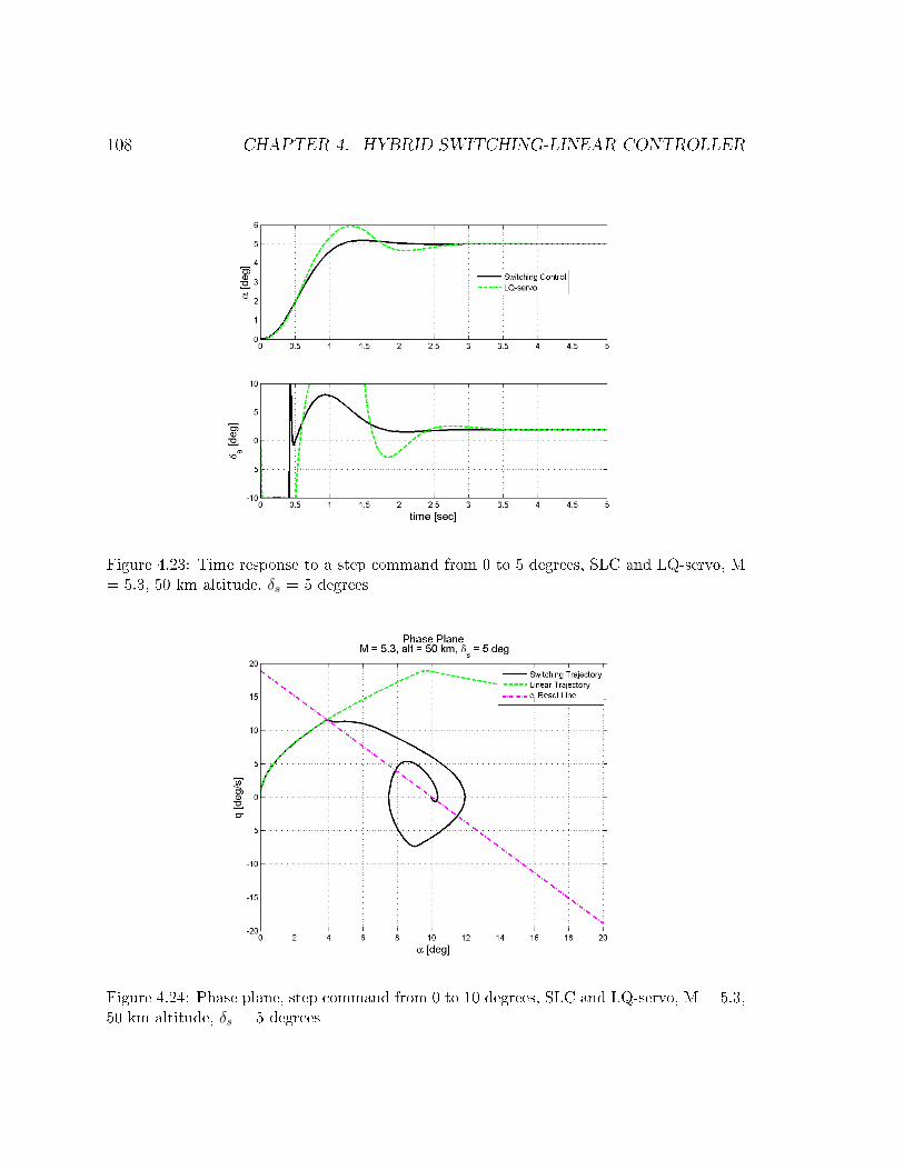
108 CHAPTER 4. HYBRID SWITCHING-LINEAR CONTROLLER
Figure 4.23: Time response to a step command from 0 to 5 degrees, SLC and LQ-servo, M
= 5.3, 50 km altitude, δs = 5 degrees
Figure 4.24: Phase plane, step command from 0 to 10 degrees, SLC and LQ-servo, M = 5.3,
50 km altitude, δs = 5 degrees
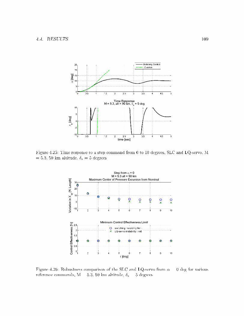
4.4. RESULTS 109
Figure 4.25: Time response to a step command from 0 to 10 degrees, SLC and LQ-servo, M
= 5.3, 50 km altitude, δs = 5 degrees
Figure 4.26: Robustness comparison of the SLC and LQ-servo from α = 0 deg for various
reference commands, M = 5.3, 50 km altitude, δs = 5 degrees

110 CHAPTER 4. HYBRID SWITCHING-LINEAR CONTROLLER
A summary of the improvement in rise time, settling time, and peak overshoot
is presented in Figure 4.27. The SLC tends to increase rise times for values of r
Figure 4.27: Time response characteristics for the SLC as a percent of the LQ-servo char-
acteristics for various step commands from 0 degrees, Mach 5.3, 50 km altitude, δs = 5
degrees
between 3 and 5 degrees, but settling time is signi�cantly reduced. The LQ-servo
controller was unable to track step commands above 5 degrees without instability;
this is re�ected in the near zero-values of rise time, settling time, and peak response
in Figure 4.27.

4.5. SLC CONCLUSIONS 111
4.5 SLC Conclusions
A hybrid switching/linear controller (SLC) was developed to improve the time re-
sponse over the linear controller. The initial phase of this controller saturates the
control input to drive the phase plane trajectory to the switching line as rapidly as
possible. At the switching line, the software state, eI , is initialized to an appropriate
value, and the LQ-servo controller controls the vehicle until the reference state is
reached.
The SLC improved the time response over the LQ-servo controller, especially
for large reference inputs. The peak overshoot and settling time were signi�cantly
decreased. The SLC was more capable at handling irregular initial states (e.g., a step
from 5 to 10 degrees) because of its error integral initialization scheme. Additionally, it
allowed the vehicle to track a 10 degree step command at Mach 5.3 and 50 km altitude,
which was not possible with the LQ-servo controller. Finally, the SLC provided this
�ight condition with some measure of robustness to uncertainty in center of pressure
location and control surface e�ectiveness. The SLC did not provide any robustness
bene�ts in static margin or control e�ectiveness for the Mach 3.5/0 km altitude or
Mach 6.3/20 km altitude cases.

This page intentionally left blank.

Chapter 5
Model Reference Adaptive Controller
The Linear Quadratic Servo controller developed in Chapter 3 performed well with
perfect plant knowledge; however, performance was degraded with reduced knowledge
of the aerodynamics. A model-reference adaptive controller (MRAC) was developed
to exploit the performance of the nominal controller while maintaining �exibility in
the face of plant uncertainty.
5.1 Theoretical Background
The author assumes the reader has a general understanding of Lyapunov stability and
Lyapunov functions. The relevant de�nitions, theorems, and proofs relating to these
topics can be found in the extensive literature on nonlinear systems (e.g., [21],[22]).
113

114 CHAPTER 5. MODEL REFERENCE ADAPTIVE CONTROLLER
Figure 5.1: Model-Reference Adaptive Control Framework
The model reference control framework is pictured in Figure 5.1. The qual-
itative control strategy involves running a �reference� model that exhibits desired
time-response characteristics. The reference states and plant states are compared to
form an error vector. Ensuring the error dynamics have a stable equilibrium point at
e = 0 guarantees the plant will converge to the (favorable) reference model behavior
after some transient. This stable error equilibrium is guaranteed by adjusting the
gains according to dynamics that satisfy a Lyapunov function.
5.2 Adaptive Control Design
The initial adaptive control design chose δs as a �xed parameter, leaving the state
di�erential equation in the form of Equation 3.12, and δa is the sole input. This

5.2. ADAPTIVE CONTROL DESIGN 115
development follows that outlined in [23] and [24]. Assuming the control input is of
form
δa = −KTx + kIeI (5.1)
where eI is de�ned in Equation 3.17, the plant can be modeled as
x = Ax + λB(−KTx + kIeI
)(5.2)
The matrix A is constant but not well-known, B is well-known, and λ is positive
but unknown. This limit on λ allows a reduced control e�ectiveness (the nominal
value for λ is 1), but does not allow control reversals.
The reference model is set as the nominal LQ-servo control with closed loop
dynamics
xref = Aref + BkeeI (5.3)
where Aref represents the nominal closed-loop dynamics
Aref = Anom −BKTLQservo (5.4)
and ke is the nominal LQ-servo gain on the error integral.
Forcing e (the error between the reference model and plant) to zero implies
that the real plant converges to the (stable and well-performing) reference plant.
Assuming there exist (unknown) constant gains K∗ and k∗I such that
Aref = A− λBK∗T (5.5)
ke = λk∗I (5.6)

116 CHAPTER 5. MODEL REFERENCE ADAPTIVE CONTROLLER
the error dynamics can be written as
e = x− xref
= Ax−Arefxref + λB(−KTx + kIeI
)−BkeeI
= Arefe− λBKTx + λBkIeI (5.7)
with
K = K−K∗
kI = kI − k∗I
Choosing the positive-de�nite Lyapunov function
L = 12eTe (5.8)
gives
L = eTArefe + eT(−λBKTx + λBkIeI
)(5.9)
The term eTArefe is negative de�nite since the eigenvalues of Aref are necessarily
left of the jω axis (see Equation 5.3), but the remainder of Equation 5.9 is not
necessarily negative de�nite (or even zero). Consequently, the Lyapunov function
must be augmented:
L = 12
(eTe + λKTΓ−1
x K + λΓ−1I kI
2)
(5.10)
where the adaptation rates, Γx and ΓI , are positive de�nite (and thus their inverses
are positive de�nite [25]). Γx is a diagonal matrix with nonzero terms on the main
diagonal. Now,
L = eTArefe + eT(−λBKTx + λBkIeI
)+ λKTΓ−1
x˙K + λΓ−1
I kI˙kI (5.11)
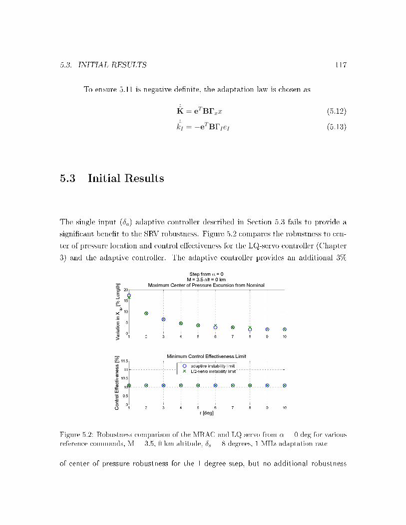
5.3. INITIAL RESULTS 117
To ensure 5.11 is negative de�nite, the adaptation law is chosen as
˙K = eTBΓxx (5.12)
˙kI = −eTBΓIeI (5.13)
5.3 Initial Results
The single input (δa) adaptive controller described in Section 5.3 fails to provide a
signi�cant bene�t to the SRV robustness. Figure 5.2 compares the robustness to cen-
ter of pressure location and control e�ectiveness for the LQ-servo controller (Chapter
3) and the adaptive controller. The adaptive controller provides an additional 3%
Figure 5.2: Robustness comparison of the MRAC and LQ-servo from α = 0 deg for various
reference commands, M = 3.5, 0 km altitude, δs = 8 degrees, 1 MHz adaptation rate
of center of pressure robustness for the 1 degree step, but no additional robustness

118 CHAPTER 5. MODEL REFERENCE ADAPTIVE CONTROLLER
at larger steps. Furthermore, the minimum allowable controller e�ectiveness is un-
a�ected. The gains stabilize at steady-state values in the face of center of pressure
uncertainty; however, the total gain variation is of the order 10−4 percent. Increasing
the adaptation rate increases allowable center of pressure variation and thus greater
gain variation, but the adaptation rate cannot be increased without bound. Proces-
sor speed, unmodeled structural modes, and unmodeled delays all limit the maximum
adaptation rate that can be sucessfully implemented on an actual system.[21]
Control surface saturation limits the adaptive controller and LQ-servo alike.
If both the adaptive and LQ-servo systems demand an asymmetric de�ection outside
the de�ection bounds, tracking will be similarly limited. A more e�ective approach
may be to control δs rather than �x it at the de�ection determined in Chapter 3.
5.4 Dual-input Adaptive Control
In the presence of controller saturation, Equation 5.2 can be written as
x = Ax + λB(δa + ∆a
)(5.14)
where δa is the commanded control de�ection and
∆a = δa − δa (5.15)
Thus, ∆a is nonzero when the commanded control de�ection, δa, is outside the
saturation limits. Alternately,
δa = δamaxsat
(δa
δamax
)(5.16)

5.4. DUAL-INPUT ADAPTIVE CONTROL 119
and
satφ =
φ, |φ| ≤ 1
1, φ > 1
−1, φ < 1
The single-input MRAC indicated control saturation hampered both LQ-servo
and adaptive control of the SRV. Ajami, Hovakimyan, and Lavretsky employ the
excess control, ∆a, to modify the reference states in the presence of saturation.[24] For
the SRV, it may be bene�cial to use the excess control to manipulate the symmetric
de�ection.
The dual-input adaptive control sought to eliminate controller saturation; that
is, ∆a → 0. The dynamics of the excess control are simply
∆a = δa − ˙δa (5.17)
Recalling the de�nitions of symmetric and asymmetric �ap de�ections (Equa-
tions 2.1 and 2.2) and the allowable range for each �ap is [0,10] degrees gives
δamax =
{2δs, δs ≤ 5
2 (10− δs) , δs ≥ 5(5.18)
and −δamax = δamin.
The obvious Lyapunov candidate function is
L = 12∆ 2
a (5.19)
which is nonzero only when the excess control is nonzero.
120 CHAPTER 5. MODEL REFERENCE ADAPTIVE CONTROLLER
Consider the case where ∆a < 0, which corresponds to δa > δamax . Then,
∆a = δamax −˙δa (5.20)
Now consider the case where ∆a > 0; that is, δa < −δamax :
∆a = −δamax −˙δa (5.21)
The time derivative of δamax can be expressed as
δamax =
{2δs, δs < 5
−2δs, δs > 5(5.22)
which is unde�ned at δs = 5. To overcome this, de�ning δamax = 0 at δs = 5 gives
δamax = 2δssign (5− δs) (5.23)
Then the time derivative of the Lyapunov candidate function in Equation 5.19
is
L = 2δs |∆a| sign (δs − 5)−∆a˙δa (5.24)
To ensure Equation 5.24 is negative de�nite, the obvious choice for δs is
δs = −ks |∆a| sign (δs − 5) + 12
˙δasign (δs − 5) sign∆a (5.25)
where ks > 0.

5.5. ADAPTIVE CONTROL CONCLUSIONS 121
Inspection of Equation 5.25 reveals a singularity at δs = 5 degrees that is
stable only when ∆a and˙δa have the same sign. This is satis�ed in two cases:
• δa is at the negative saturation limit AND the commanded de�ection is increas-
ing
• δa is at the positive saturation limit AND the commanded de�ection is decreas-
ing
Obviously, these conditions are not guaranteed. Furthermore, the sign (δs − 5) terms
in Equation 5.25 ensure the symmetric de�ections cannot move upon reaching 5 de-
grees.
In the future, it may be possible to augment the Lyapunov function in Equation
5.19 with additional terms to remove the singularity at δs = 5.
5.5 Adaptive Control Conclusions
A model-reference adaptive controller was developed to control the asymmetric de-
�ection while maintaining a �xed symmetric de�ection. This single-input, single-
output system approach paralleled the approach developed in the previous chapters.
The adaptive control failed to provide any additional appreciable robustness over the
baseline LQ-servo controller of Chapter 3. Small gains in robustness to center of
pressure variation were demonstrated for small reference commands and clock speeds

122 CHAPTER 5. MODEL REFERENCE ADAPTIVE CONTROLLER
of 1 MHz. The control saturation e�ects that limited the linear controller likewise
hampered the e�ectiveness of the adaptive controller.
In an initial attempt to alleviate some saturation problems, an additional
adaptive controller was designed to drive the control saturation to zero. The control
scheme presented above was unsuccessful at ensuring stability, but a similar approach
may prove useful in future work. The major di�culty in designing such a dual-input
adaptive controller is the choice of a satisfactory Lyapunov function candidate and
associated control strategy.
The dual-input adaptive controller presented treated the control of the asym-
metric de�ection, δa, as independent of the symmetric de�ection, δs. Then, δs was
modulated to alleviate the saturation on δa. A more suitable approach may be to
treat both inputs simultaneously.
Chapter 6
Conclusions
6.1 Summary
The primary objective of this research was to design an angle of attack tracking
controller for a variable-stability slender reentry vehicle (SRV). The vehicle was con-
trolled by two �aps mounted near the base of the 2-dimensional, wedge-shaped (or
3-dimensional, conical) vehicle. These �aps altered both the pitch static stability
and trim characteristics of the vehicle through two separate control inputs: symmet-
ric �ap de�ection and asymmetric �ap de�ection, respectively. This �ap controlled
con�guration had signi�cant control de�ection limits that introduced nonlinearity to
the system. Additionally, the symmetric de�ection input entered the equation of mo-
tion nonlinearly and coupled with the angle of attack. In practice, the aerodynamic
data of the SRV may be poorly known. Speci�cally, this e�ort assumed the center
of pressure location may be poorly known, control surfaces may experience ablation
123

124 CHAPTER 6. CONCLUSIONS
and reduced e�ectiveness, and asymmetric ablation may induce a nonzero pitching
acceleration (speci�c moment) on the vehicle.
A linear quadratic servo (LQ-servo) tracking controller was designed that aug-
mented the two pitch states (angle of attack and pitch rate) with the integrated
tracking error. Three design points along a typical ballistic reentry trajectory were
selected for controller analysis: Mach 5.3 and 50 km altitude, Mach 6.3 and 20 km
altitude, and Mach 3.5 and 0 km altitude. The LQ-servo was selected because it
enjoys guaranteed stability and robustness margins in the absence of nonlinearities.
For whole-number symmetric de�ections from 2 degrees to 8 degrees, the LQ-servo
was designed to meet a speci�ed rise time and gain margin. Robustness to center of
pressure variation, reduced control e�ectiveness, and unmodeled pitch accelerations
were determined. The addition of a �rst order actuator reduced vehicle tracking per-
formance when vehicle dynamics were relatively fast (high dynamic pressures). A
lead compensator demonstrated the ability to alleviate some of the actuator-caused
performance degradation. Robustness to center of pressure variation at high dynamic
pressures was correlated with the linear instability limits, while nonlinear control
saturation e�ects limited the robustness at low dynamic pressures or large reference
commands. Additionally, low dynamic pressure reduced the the system tolerance for
less e�ective controls and external pitch accelerations. A symmetric de�ection was
selected at each �ight condition that maximized robustness and demonstrated favor-
able time responses at both 1 degree and 10 degree step commands in reference angle
of attack.
A hybrid switching linear controller (SLC) was designed to exploit the favor-
able performance of the LQ-servo but improve the time response and robust per-
formance, especially for large reference commands. The LQ-servo phase plane was
analyzed for regions of satisfactory and unsatisfactory performance. A region of satis-
factory, unsaturated LQ-servo performance was determined, and a linear initialization
of the integrated tracking error was designed along this region. Outside the LQ-servo

6.2. RECOMMENDATIONS FUTURE RESEARCH 125
region, a saturated controller employs the maximum de�ection to drive the phase
plane trajectory to the LQ-servo region. The SLC reduced settling times, especially
for large reference commands and nonzero initial angles of attack. The SLC did not
provide additional robustness for the Mach 3.5, 0 km altitude or Mach 6.3, 20 km
altitude case; however, the SLC did allow large reference commands to be tracked at
Mach 5.3, 50 km altitude that were unstable with the LQ-servo controller.
With the goal of improving robustness, a model-reference adaptive controller
(MRAC) was developed. The MRAC attempted to match the performance of the
nominal system controlled by the LQ-servo controller. The adaptive controller did not
provide additional robustness over the LQ-servo controller because control saturation
e�ects continued to limit performance. An initial attempt to design a dual-input
adaptive control for both the symmetric and asymmetric de�ections was described;
however, the Lyapunov candidate function and control scheme did not guarantee
stability for all symmetric de�ections.
6.2 Recommendations Future Research
The SLC was dependent on accurate center of pressure knowledge (up to 2% of the
length for large reference commands). In reality, the static margin is not likely to be
known a priori within these margins. Consequently, on-line estimation of the static
margin may be necessary. A small angle of attack oscillation command may be useful
in estimation of the static margin. With a more accurate static margin, the control
strategy (LQ-servo gains, switching curve, etc.) may be adjusted on-line as static
margin knowledge improves.

126 CHAPTER 6. CONCLUSIONS
An adaptive controller may be useful in adjusting to plant uncertainty, but the
single-input controller developed was still limited to �ight pro�le-scheduled symmetric
de�ections. Furthermore, the control saturations still limited the adaptive controller.
It may be possible to design an adaptive controller that manipulates the symmetric
de�ection based on control saturation. The dual-input scheme similar to that pre-
sented in Section 5.4 can potentially provide a means to control both symmetric and
asymmetric de�ections during reference-command tracking. On the other hand, it
may be bene�cial to design a controller that simultaneously controls both δs and δa,
rather than employing independent adaptations. An adaptation on the SLC switching
line and integrated tracking error initialization may provide additional robustness.

Bibliography
[1] Bertin, J. J., Hypersonic Aerothermodynamics , AIAA, Washington D.C., 1994.
[2] Kolodziej, P., Bowles, J. V., and Roberts, C., �Optimizing hypersonic sharp bodyconcepts from a thermal protection system perspective,� AIAA International
Space Planes and Hypersonic Systems and Technologies Conference, April 27�301998, pp. 556�571.
[3] Cavallo, A., De Maria, G., and Ferrara, F., �Attitude control for low lift/dragre-entry vehicles,� Journal of Guidance, Control, and Dynamics , Vol. 19, No. 4,1965, pp. 816�822.
[4] Dukeman, G., �Pro�le-Following Entry Guidance Using Linear Quadratic Regu-lator Theory,� AIAA Guidance, Navigation, and Control Conference and Exhibit ,August 2002.
[5] Bibeau, R. and Rubinstein, D., �Trajectory optimization for a �xed-trim reentryvehicle using direct collocation and nonlinear programming,� AIAA Guidance,
Navigation, and Control Conference and Exhibit , August 2000.
[6] Juliana, S., Chu, Q., Mulder, A., and van Baten, T., �Nonlinear Flight Controlfor Re-entry Flight Vehicle,� 55th International Astronautical Congress , August2004.
[7] Mooij, E., Mease, K., and Benito, J., �Robust Re-Entry Guidance and ControlSystem Design and Analysis,� AIAA Guidance, Navigation, and Control Con-
ference and Exhibit , August 2007.
127

128 BIBLIOGRAPHY
[8] Lu, P., �Entry Guidance and Trajectory Control for Reusable Launch Vehicle,�Journal of Guidance, Control, and Dynamics , Vol. 20, No. 1, 1965, pp. 143�149.
[9] Shtessel, Y., Tournes, C., and Krupp, D., �Reusable launch vehicle control in slid-ing modes,� AIAA Guidance, Navigation, and Control Conference, New Orleans,LA, August 11�13 1997.
[10] Burkhardt, J. and Schoettle, U. M., �Flight performance and control aspects of asemi-ballistic reentry capsule,� Atmospheric Flight Mechanics Conference, July29�31 1996.
[11] Casey, J. J., �In�uence of ablation on the dynamics of slender re-entry con�gu-rations,� Journal of Spacecraft and Rockets , Vol. 2, No. 1, 1965, pp. 106�108.
[12] Bertin, J. J., Aerodynamics for Engineers , Prentice Hall, Upper Saddle River,NJ, 4th ed., 2002.
[13] Chamito�, G., Robust Intelligent Flight Control for Hypersonic Vehicles , Ph.D.thesis, Massachusetts Institute of Technology, 1992.
[14] Etkin, B., Dynamics of Atmospheric Flight , John Wiley & Sons, Toronto, On-tario, 1972.
[15] Shampine, L. F. and Reichelt, M. W., �The MATLAB ODE Suite,� SIAM Jour-
nal on Scienti�c Computing , Vol. 18, 1997, pp. 1�22.
[16] Shampine, L. F., Reichelt, M. W., and Kierzenka, J., �Solving Index-1 DAEs inMATLAB and Simulink,� SIAM Review , Vol. 41, 1999, pp. 538�552.
[17] Arthur E. Bryson, J. and Ho, Y.-C., Applied Optimal control: Optimization, Es-
timation, and Control , Hemisphere Publishing Corporation, Washington, D.C.,1975.
[18] Kirk, D. E., Optimal Control Theory: An Introduction, Dover, Mineola, NY,1998.
[19] Stengel, R. F., Optimal Control and Estimation, Dover, Mineola, NY, 1994.
[20] Yechout, T., Morris, S., Bossert, D., and Hallgren, W., Introduction to Aircraft
Flight Mechanics: Performance, Static Stability, Dynamic Stability, and Calssi-
cal Feedback Control , AIAA, Reston, VA, 2003.
[21] Slotine, J.-J. E. and Li, W., Applied Nonlinear Control , Prentice Hall, UpperSaddle River, NJ, 1991.

BIBLIOGRAPHY 129
[22] Vidyasagar, M., Nonlinear Systems Analysis , SIAM Publications, Philadelphia,2nd ed., 2002.
[23] Lavretsky, E. and Hovakimyan, N., �Stable Adaptation in the Presence of Actua-tor Constraints with Flight Control Applications,� Journal of Guidance, Control,and Dynamics , Vol. 30, No. 2, 2007, pp. 337�345.
[24] Ajami, A., Hovakimyan, N., and Lavretsky, E., �Design examples: AdaptiveTracking Control in the Presence of Input Constraints for a Fighter Aircraft anda Generic Missile,� AIAA Guidance, Navigation, and Control Conference, SanFrancisco, CA, August 15�18 200.
[25] Strang, G., Applied Linear Algebra, Wellesley-Cambridge Press, Welleslye, MA,1986.
[26] Brandt, S., Stiles, R., Bertin, J., and Whitford, R., Introduction to Aeronautics:
A Design Perspective, AIAA, Reston, VA, 1997.
[27] Hillje, E. R., �Entry Aerodynamics at Lunar Return Conditions,� NASA Tech-nical Note TN D-5399, NASA, October 1969.
[28] Wingrove, R., �Trajectory Control Problems in Planetary Entry of Manned Ve-hicles,� Journal of Spacecraft and Rockets , Vol. 2, No. 6, 1965, pp. 883�886.

This page intentionally left blank.
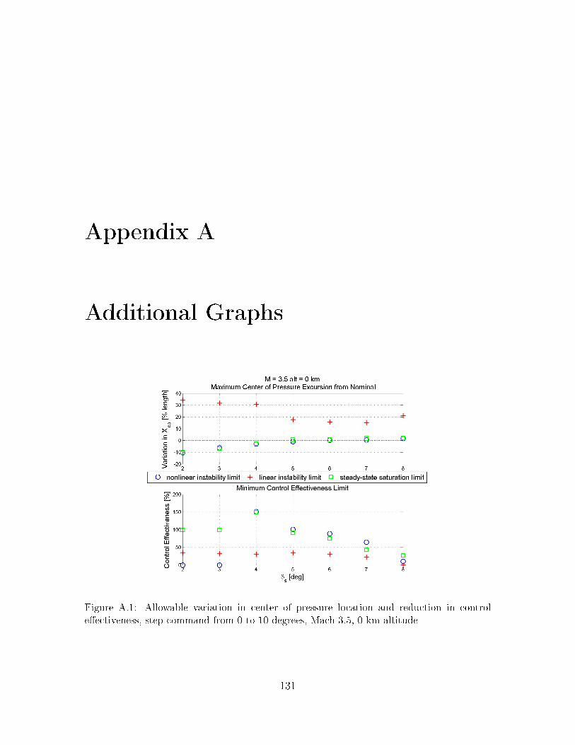
Appendix A
Additional Graphs
Figure A.1: Allowable variation in center of pressure location and reduction in control
e�ectiveness, step command from 0 to 10 degrees, Mach 3.5, 0 km altitude
131
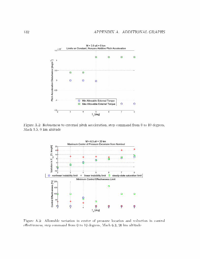
132 APPENDIX A. ADDITIONAL GRAPHS
Figure A.2: Robustness to external pitch acceleration, step command from 0 to 10 degrees,
Mach 3.5, 0 km altitude
Figure A.3: Allowable variation in center of pressure location and reduction in control
e�ectiveness, step command from 0 to 10 degrees, Mach 6.3, 20 km altitude

133
Figure A.4: Robustness to external pitch acceleration, step command from 0 to 10 degrees,
Mach 6.3, 20 km altitude
Figure A.5: Allowable variation in center of pressure location and reduction in control
e�ectiveness, step command from 0 to 10 degrees, Mach 5.3, 50 km altitude

134 APPENDIX A. ADDITIONAL GRAPHS
Figure A.6: Robustness to external pitch acceleration, step command from 0 to 10 degrees,
Mach 5.3, 50 km altitude
Figure A.7: Time response characteristics for step commands from 0 degrees, Mach 6.3, 20
km altitude, 1st order actuator Modeled
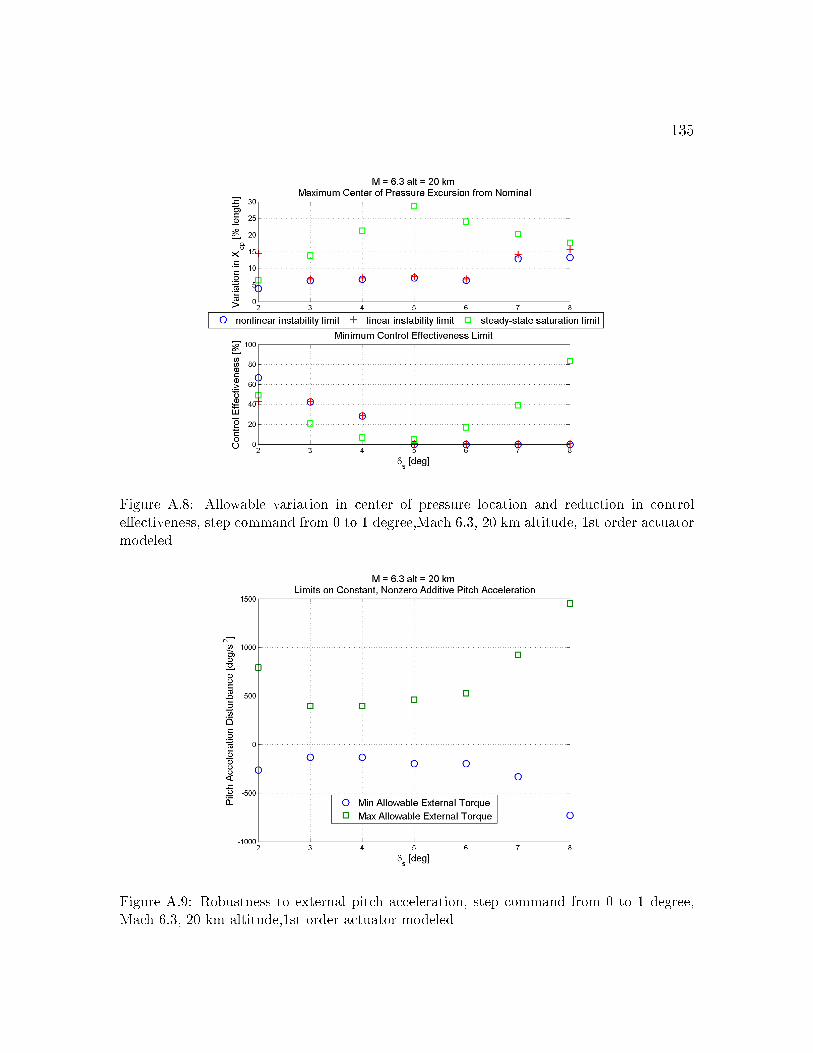
135
Figure A.8: Allowable variation in center of pressure location and reduction in control
e�ectiveness, step command from 0 to 1 degree,Mach 6.3, 20 km altitude, 1st order actuator
modeled
Figure A.9: Robustness to external pitch acceleration, step command from 0 to 1 degree,
Mach 6.3, 20 km altitude,1st order actuator modeled
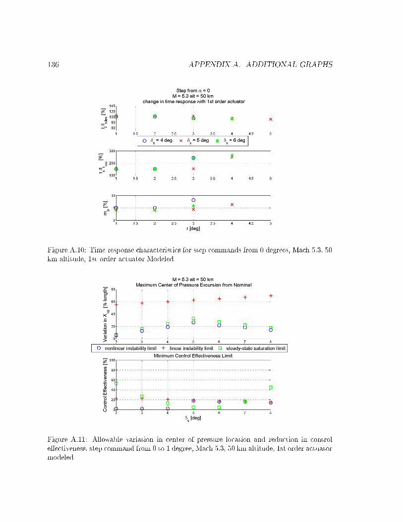
136 APPENDIX A. ADDITIONAL GRAPHS
Figure A.10: Time response characteristics for step commands from 0 degrees, Mach 5.3, 50
km altitude, 1st order actuator Modeled
Figure A.11: Allowable variation in center of pressure location and reduction in control
e�ectiveness, step command from 0 to 1 degree, Mach 5.3, 50 km altitude, 1st order actuator
modeled

137
Figure A.12: Robustness to external pitch acceleration, step command from 0 to 1 degree,
Mach 5.3, 50 km altitude, 1st order actuator modeled