Temporary Workers, Uncertainty and Productivity∗

Francesca Lotti and Eliana VivianoBank of Italy

October 8, 2012

Abstract

Hiring temporary workers can be viewed as a real option which allows firmsto adjust labor input as economic conditions fluctuate and uncertainty aboutfuture demand increases. The “purchase price” of this real option may be,among other things, lower productivity. We develop a dynamic model of labordemand with uncertainty that allows us to draw some testable predictions onthe level and on the composition of the labor force, according to the level ofuncertainty. Using a panel of Italian firms, which collects also a measure of firm-specific uncertainty, we first present evidence that firms adjust the workforcesize and composition according to uncertainty. Second, using a set of reforms ofpermanent and temporary employment, we estimate the relationship betweenTFP and permanent employment. We find that incentives to hire permanentworkers positively affect TFP. This effect is stronger for firms facing higheruncertainty, as those belonging to high-tech sectors.

JEL classification: J21, J23, D81.Keywords: fixed-term workers, uncertainty, productivity, real options.

∗We are grateful to Joshua Angrist, Andrea Brandolini, David Card, Francesco D’Amuri, Alessan-dro Sembenelli, Paolo Sestito, Alfonso Rosolia, Roberto Torrini and the participants to variousworkshops and seminars for their comments on previous versions of the paper. The views expressedhere are those of the authors and do not necessarily reflects those of the Bank of Italy. The usualdisclaimers apply.

1 Introduction

In the last two decades, aimed at reducing unemployment rates, many European

countries have undertaken a series of reforms in the labor market in order to increase

flexibility “at the margin”. These reforms have deeply changed the European labor

market and their effects have been studied from many different viewpoints.

One strand of the literature focuses on the employment effect of such reforms

trying to assess empirically if labor markets are segmented and/or whether temporary

employment arrangements are stepping stones to find a suitable and permanent job

in the future (e.g. Ichino and Riphahan, 2005). More recently, increasing attention

has been paid to the implications for the firms, often finding a negative relationship

between the use of temporary work arrangements and productivity (e.g. Autor, Kerr

and Kugler, 2007; Dolado, Ortigueira and Stucchi, 2012; Cappellari, Dell’Aringa and

Leonardi, 2012).

These results, however, impose a simple question. Why do firms hire temporary

workers then? Undoubtedly, for firms there is an evident trade off between the opti-

mal labor input choice and productivity levels. In this spirit, the contribution of this

paper is to show that there is an economic rationale behind hiring temporary workers,

if they are viewed as a kind of real option for firms. Since hiring permanent workers

implies irreversible costs due to employment protection legislation, when demand un-

certainty increases, firms may find convenient to postpone the decision to hire workers

permanently. This idea is not new: Dixit and Pindyck proposed it in their textbook

“Investment under Uncertainty” edited in 1994. They argue that after the recession

of early Nineties, permanent full-time hiring increased slowly because a high level

of uncertainty about future demand, which forced US firms to wait before make the

commitment involved in hiring permanent workers. In the meantime, they preferred

to exploit the current profit opportunities using less irreversible and sometimes more

costly (or less efficient) inputs of production, like temporary work, mainly in the form

of employment-agency placement. Foote and Folta (2002) explicitly claim that the

low productivity associated to hiring temporary workers is the cost of the real option

of a lower degree of irreversibility.

The contribution of our paper is to derive a dynamic model of labor demand with

2

uncertainty, where labor is treated as a quasi-irreversible input. Aimed at under-

standing the role of uncertainty on the level and on the composition (in terms of

permanent and temporary workers) of the workforce, we calibrate the model in order

to identify one regime with low and one with high uncertainty. Higher uncertainty

enlarges the so called “inaction area”, i.e. when firm postpones any decision on labor

force adjustment; higher uncertainty reduces hirings, both of temporary and perma-

nent workers, but less so for temporary; workers with a closed-end contract - an input

completely reversible - are employed as a buffer. We then test these model predic-

tions with an empirical analysis based on a panel of Italian firms for which we have

a measure of perceived current output demand uncertainty, along with a measure of

productivity for the period that goes from 1999 to 2010.

We carry out two types of empirical exercises. First, we analyze the relationship

between firm uncertainty and labor demand growth and composition. Our identi-

fication strategy is based on the assumption that firm uncertainty is a firm-specific

time-invariant characteristic. Thus, to each firm we assign a measure of uncertainty

equal to the level of reported uncertainty about current output demand at the begin-

ning of the period. We then model labor demand as a function of uncertainty and

time, sector and region fixed effects. Our main identification assumption is that un-

certainty in 1999 affects future labor demand, but the realization of labor demand in

the year after 1999 does not affect firm’s uncertainty in that year. We find that when

uncertainty increases, total labor demand decreases, while the share of temporary

workers in total workforce grows.

Second, we would like to verify that firms facing higher uncertainty face also lower

TFP, not only because higher uncertainty has a direct effect on TFP, but also because

uncertainty increases the incentives to hire temporary workers and temporary workers

have a direct negative effect on TFP. To carry out this exercise we need an exogenous

source of variation for the incentive to hire temporary workers. Following Cipollone

and Guelfi (2002) and Cappellari, Dell’Aringa and Leonardi (2012), we rely on the

fact that after 2001 the Italian government undertook several different reforms aimed

at reducing the social contributions paid to hire young permanent workers and at

the same time ease the use of temporary work arrangements (the so-called “Biagi

3

Law” of 2003). These interventions exhibits time, regional and sectoral variation. We

then derive a variable which captures the disincentive to use closed-end contracts to

isolate the effects of these workers on firms’ TFP. Also, we control for our measure

of uncertainty and for the interaction between uncertainty and the use of fixed term

contracts. We find, in line with the previous literature, that TFP is negatively affected

by the use of fixed term workers. As suggested by the theory, also uncertainty has

a direct and negative effect on TFP. Moreover, the effect of temporary workers on

TFP is not uniform across firms, but varies according to the firm-specific uncertainty.

Going from the 10th percentile to the 90th percentile of the distribution of uncertainty

(a difference equal to 0.17), TFP, on average, decreases by 11 per cent. The incentive

to hire permanent workers contributes to the TFP increase for firms facing extremely

high uncertainty by roughly 4 percentage points; on the contrary, it has virtually no

effect for firms facing very low uncertainty.

Our framework differs from the one proposed by Boeri and Garibaldi (2007), who

find a negative relationship between the share of closed-end contracts and firms’ pro-

ductivity growth. They interpret this result in terms of a transitory increase in labor

demand induced by the higher flexibility of temporary jobs (the so-called “honeymoon

effect”). They derive a model of labor demand with uncertainty, which encompasses

a transition from a rigid to a two tier system. The introduction of the new regime,

features a honeymoon effect that involves an increase in the share of firms able to

adjust their employment levels, a temporary positive effect on average employment,

and a temporary negative effect on average productivity because, under the decreasing

marginal returns to labor hypothesis, firms hire increasingly less productive workers

with closed-end contracts. Other papers investigate the relationship between TFP

and temporary employment. Dolado, Ortigueira and Stucchi (2012) model a labor

market where labor costs vary by type of job contract. They also present evidence

based on Spanish data that higher shares of temporary workers decrease firms’ total

factor productivity. On a similar perspective, Bird and Knopf (2009) analyze the

effects of wrongful-discharge protections on earnings, profitability and efficiency of

the US banking sector, finding that a higher employment protection legislation raises

wages, reduces profits and lowers productivity. Using time and geographical varia-

4

tion in employment protection legislation, Autor, Kerr and Kugler (2007) find that

for the US, the introduction of employment protection legislation reduces produc-

tivity by distorting production choices. A higher employment protection legislation

would trigger an excessively intensive capital deepening (with respect to optimal in-

put choice of an hypothetical production function). However, they also find that that

labor productivity rose substantially following adoption of new employment protec-

tion legislation. Similarly, Acharya, Baghai and Subramanian (2009) find that in the

US strong dismissal laws appear to have a positive effect on the innovative pursuits

of firms and their employees. Based on UK data, Michie and Sheenan (2003) find

that the use of temporary workers along with little training (the so-called “low-road”

practices to human resource management) is negatively correlated with productivity

growth. A similar result is found by Kleinknecht et al. (2006) for the Netherlands:

the employment growth in the Eighties and in the Nineties, occurred by means of tem-

porary workers, is followed by a remarkable productivity slowdown. More recently

for Italy, Cappellari, Dell’Aringa and Leonardi (2012) find not only that temporary

work arrangements negatively affect TFP, but also that the effect differ across tem-

porary job contracts: those associated to some training activity, like apprenticeship

have instead a positive impact on TFP (confirming indirectly the “low-road” practice

hypothesis).

The paper is organized as follows. Section 2 describes the dynamic model of

labor demand with uncertainty, for which we derive some testable implications, while

Section 3 is devoted to a description of the data for the empirical testing. Section 4

deals with the effects of uncertainty on labor demand and workforce composition. In

Section 5 the relationship between the share of temporary workers and productivity.

Section 7 split the results by high and low tech sectors as these two sectors are

characterized by different level of uncertainty. Section 7 further investigates possible

differences across high and low tech sectors. Finally, Section 8 briefly concludes.

5

2 A Model of Labor Demand with Uncertainty

As in the standard models of investment under uncertainty, we consider a represen-

tative single product firm with homogeneous inputs (e.g. Bloom et al., 2007). Firm’s

decisions on investment are partially irreversible, and under uncertainty irreversibility

generates real options on the investment decisions with a typical separation of the

thresholds for investment and disinvestment, with no action undertaken between the

thresholds.

Our model of labor demand is based on a very stylized Cobb-Douglas production

function with two kinds of labor input, permanent and temporary workers, and is

similar to the one developed by Chen and Funke (2009). Since we are interested

in firms’ behavior concerning labor adjustment, we assume that i) physical capital

is fixed and firms do not invest, so that the real option term can be univocally at-

tributed to permanent workers’ hirings and ii) there is no entry/exit in the market,

that would require more computational complexity in the model.

The production function of the representative firm is:

Yt = At ·KαKt · LαPP,t · L

αTT,t (1)

where K is physical capital, LT and LP are temporary and permanent workers, re-

spectively. The firm faces an isoelastic demand curve:

pt = Y1−ρρ

t × Zt (2)

where p is the price of the good, ρ ≥ 1 and Zt is the demand shock that follows a

geometric Brownian motion of the following kind:

dZt = ηZtdt+ σZtdWt (3)

where Wt is a Wiener process with independent, normally distributed increments, η is

a deterministic drift parameter, and σ is the volatility parameter, so that the demand

for the good produced is subject to uncertainty.

From the theory about investment under uncertainty it is well known that when

6

an input is irreversible, a firm’s optimal investment rule takes on a threshold form.

Adjustment of the labor force when subject to hiring and firing costs will only occur

when demand hits some thresholds. It has been well documented that because uncer-

tainty raises the upper threshold for investment (the hiring threshold in this specific

case), it reduces the rate of investment, with evident loss of efficiency.1

Firm’s profits at time t are defined as:

π = A1ρK

αKρ L

αPρ

P LαTρ

T Z − wPLP − wTLT − CP (∆LP ) − CT (∆LT ) (4)

where wP and wT are wages for permanent and temporary workers respectively and

CP (·) and CT (·) are the labor adjustment cost functions (the subscript t is omitted

to avoid cumbersome notation). Since the framework production function is a Cobb-

Douglas, wP and wT also represent the marginal product of the two kind of workers.

Without loss of generality, we assume that, in case of temporary workers, there

are no adjustment costs, so that we will set CT (·) = 0. For the sake of tractability,

adjustment costs for permanent workers are symmetric and convex functions:

CP (∆LP ) =

cf + bf∆LP + 12λf (∆LP )2 if ∆LP < 0 (firings)

ch + bh∆LP + 12λh (∆LP )2 if ∆LP > 0 (hirings)

0 if ∆LP = 0 (no change)

(5)

where cf/h are fixed costs components for firing and hiring, respectively, bf/h are the

unit costs of adjusting the size of the workforce and λf/h are the adjustment speed

parameters.

1The effect of uncertainty in raising the investment threshold is demonstrated, for example, byPindyck (1988), Dixit (1989), Bentolila and Bertola (1990), Bertola and Caballero (1994), Dixit andPindyck (1994) and Abel and Eberly (1996).

7

Given that r is the rate of return, firms maximize the present discounted value of

their current and future stream of profits according to:

V = maxLP

∫ ∞0

[A

1ρK

αKρ L

αPρ

P LαTρ

T Zt − wPLP − wTLT − CP (∆LP )

]exp−rs ds (6)

Applying Ito’s Lemma, equation (6) becomes:

rV = A1ρK

αKρ L

αPρ

P LαTρ

T Zt − wPLP − wTLT − CP (∆LP ) + ηZV Z +1

2σ2V ZZZ2 (7)

where V Z is the derivative of V with respect to Z. The firm’s optimal permanent and

temporary levels of employment are obtained maximizing the expected discounted

value of the future cash flow. Since temporary workers can be terminated at the

end of the job contract at no cost, there is neither a real option term associated to

hiring or firing them, nor a dynamic effect in firm’s choice. Clearly, the model has

no closed form; nevertheless it is possible to derive threshold levels for hiring/firing

and by means of calibration it is possible to see how the firm’s choice on the mix of

temporary and permanent employment changes with demand uncertainty.

The first order condition for employment changes yields:

±bh/f + λh/f∆LP = ν (8)

where ν is the derivative of the value function (6) with respect to LP . Substituting

the cost function depicted in equation (5) into equation (7) and rearranging, we derive

firing and hiring decisions for permanent workers.The hiring (firing) thresholds are

derived finding the value of ν for which an additional worker (one worker less) would

generate negative profits, leading to the following thresholds:

ν = bh +

√(2chλh

)for hiring thresholds (9)

8

ν = −bf −

√(2cfλf

)for firing thresholds (10)

Given the structure of our model, the “inaction zone”, i.e. the region where no

hirings and firings occur because the demand shock is not large enough to compensate

the costs of adjustment, is

−

√(2cfλf

)≤ ∆LP ≤

√(2chλh

)(11)

The larger the fixed costs, the wider the inaction area is: the firm does not hire/fire

until the number of hirings/firings covers the fixed costs. Also the adjustment speed

parameter affect the inaction area: smaller values of λh/f would imply a smaller

inaction area.

The first order condition for temporary employment LT is the derivative of equation

(4) with respect to LT : it reduces to a simple function of the demand shock Z and

the level of permanent employment LP .

αTρA

1ρK

αKρ L

αPρ

P LαTρ−1

T Z − wT = 0

LT =

wT

αTρA

1ρK

αKρ L

αPρ

P Z

ρ

αT+ρ

(12)

When the demand shock is positive and large enough to approach the hiring

threshold, the firm will hire temporary workers first, and permanent employees after.

Symmetrically, as the demand shock is as negative as to hit firing thresholds, the

firm will adjust workers with a closed-end contract first and permanent employees

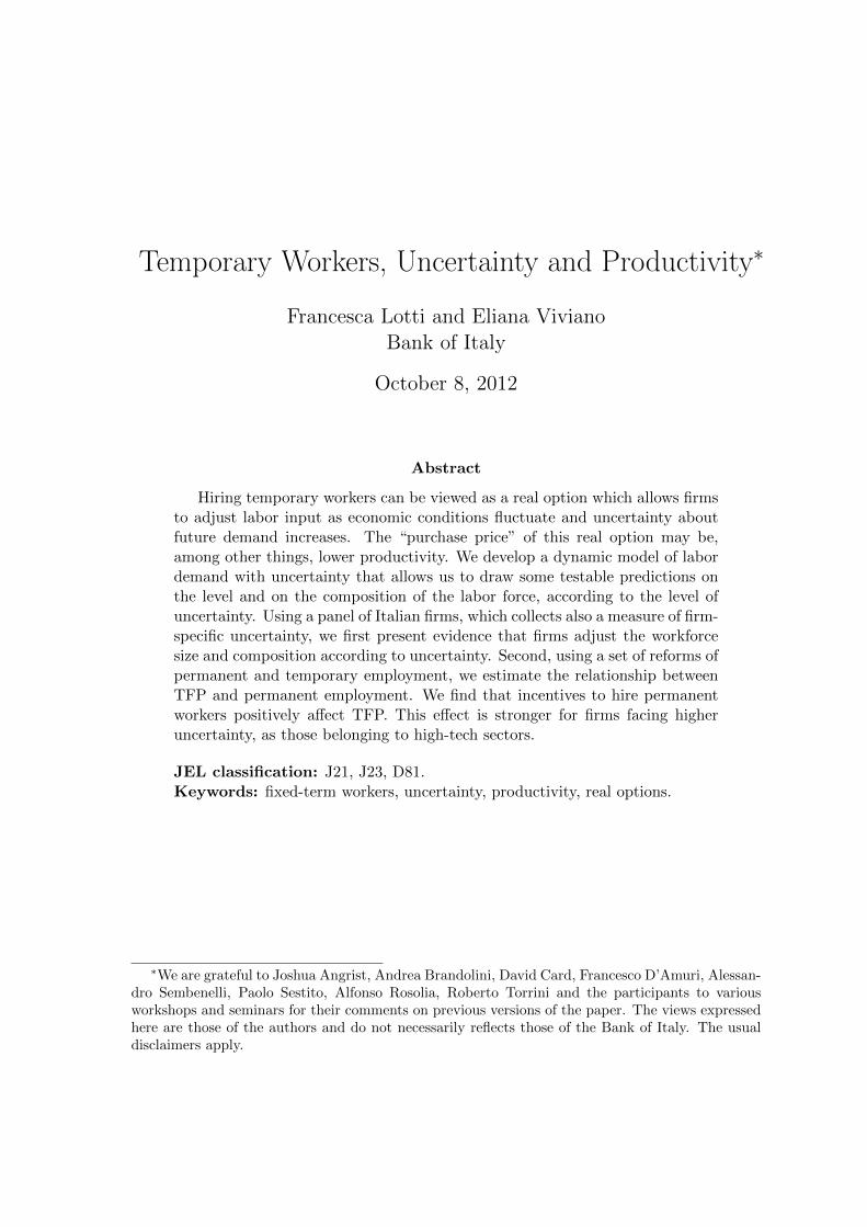
subsequently. In summary, the availability of temporary workers widens the inaction

area and serves as a buffer to adjust labor force - quickly and cheaply - to unexpected

demand fluctuations, as reported on Figure 1 .

9

As mentioned above, we are mainly interested to understand how uncertainty,

proxied by the volatility parameter σ in equation (3), affects the number of hirings

and their composition, in terms of open and closed-end contracts. To do so, we cal-

ibrate the model as indicated on Table (1), with σ that takes two possible values,

one for a low uncertainty regime (σ = 0.15) and one for a high uncertainty regime

(σ = 0.25). Moreover, we assume that wages are the same for permanent and tempo-

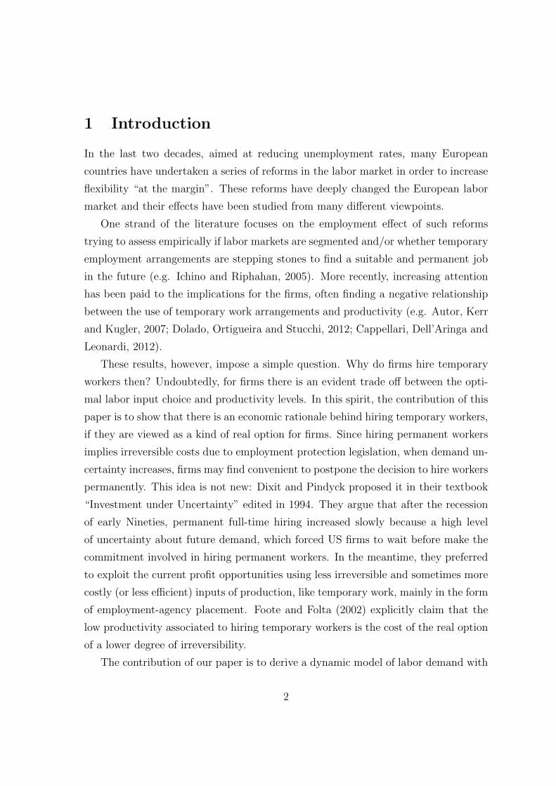
rary workers.2 Hiring and firing thresholds are depicted on Figure (2). Consistently

with the rigidity of the Italian labor market, the model has been calibrated in such a

way that hiring and firing thresholds are never symmetric, with the firing threshold

being more flat the the hiring threshold. High levels of uncertainty make the firing

threshold even more flatter, while hiring thresholds become steeper with higher un-

certainty.

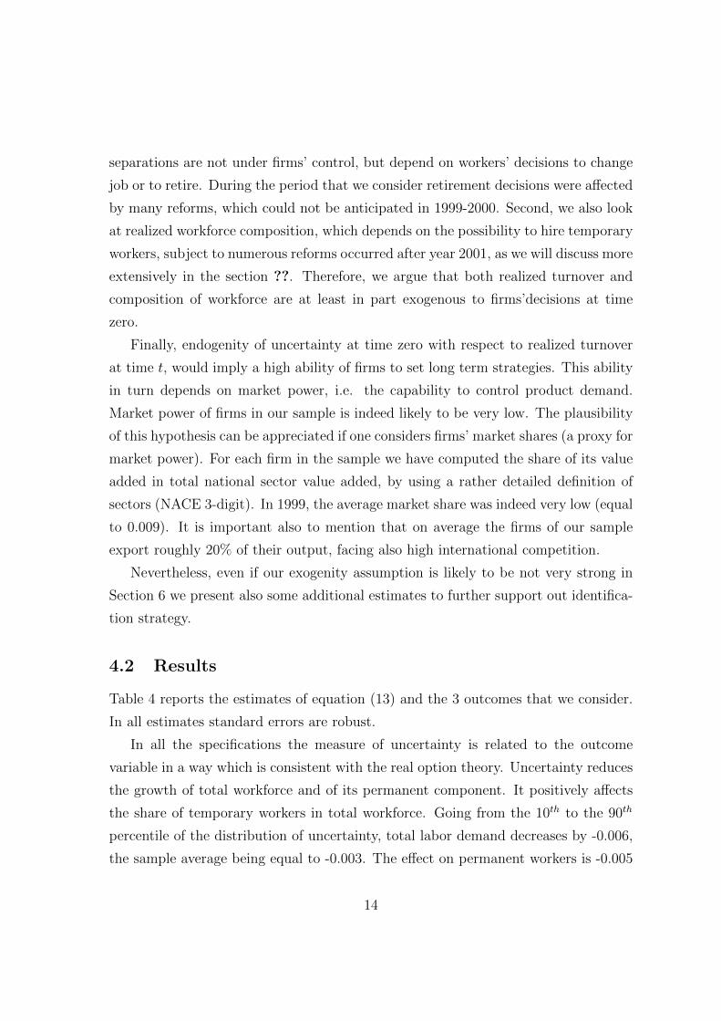
Based on the aforementioned calibrations, the stylized model allows us to draw some

testable implications, based on the graphical evidence depicted on Figure (3):

Hypothesis 1: when uncertainty increases, the number of total hirings decreases;

Hypothesis 2: when uncertainty increases, the number of temporary hirings de-

creases, but seemingly less so with respect to permanent hirings. Consequently, the

share of temporary workers in total workforce increases;

Hypothesis 3: when uncertainty increases, the number of permanent hirings de-

creases;

Hypothesis 4: when uncertainty increases and the “inaction area” becomes larger,

preventing firms to adjust labor force to demand conditions, therefore undermining

their efficiency (hence productivity).

The next section is devoted to test empirically these hypotheses on a sample of

Italian manufacturing firms for the 1999-2010 period.

2We also calibrated the model with different wages, in particular we set wT = 0.8wP , but theresults are confirmed.

10

3 The Data

The data used in the empirical analysis come from two sources. The first is the Bank

of Italy yearly survey on industrial and non financial service firms with more than 20

employees (INVIND, hereinafter). The survey collects data on the most relevant vari-

ables on company activities, like investment, sales, ICT expenditure, price changes,

firm’s strategies, and, more importantly, detailed information on employment, such

as yearly average job flows and their composition, i.e. permanent vs. temporary

workers.3. The sample is stratified according to firms’ branch of activity, size class

and geographical areas. Along with information on the reference year, which is the

one prior to the interview, firms are also required to report their expectations on

turnover and prices for the current year, which allow us to get estimates of the ex-

pected real demand change and to estimate ex post also the size of the unexpected

demand shock. Firms are also asked to report an upper and a lower bound for their

expected real demand change: these bounds can be used to proxy the volatility of

the expected demand, which is bounded from above by the squared of the difference

between the upper and the lower bounds. This measure of uncertainty have been

used, for instance, to show how capital investments respond to firm-specific uncer-

tainty (e.g. Guiso and Parigi, 1999). For the purpose of this paper, we select only

manufacturing firms which started participating in the survey between 1999 and 2001,

until 2010 (or until the time of leaving the sample).

The second dataset that we use is the Company Accounts Data Service (CADS)

that collects balance sheet information on a large sample of firms, with a very good

coverage of large firms (see also Pistaferri, Guiso and Schivardi, forthcoming, for

further details). Using balance sheet information, it is possible to build a measure

of capital stock, by means of the perpetual inventory method, and to estimate firm

level total factor productivity (TFP) with the methodology proposed by Levinsohn

and Petrin (2003) that, using intermediate input purchases as a control function,

allows us to obtain TFP estimates that do not suffer from the common selectivity

and simultaneity problems.

3In Italy there are many different types of closed-end job contracts, but our data do not allow usto distinguish them by type, as done by Cappellari, Dell’Aringa and Leonardi, 2012.

11

Table 2 reports the characteristics of the sample used in the empirical analysis and

some statistics on selected variables: total net hires (i.e. minus fires) normalized by

total workforce, net percentage growth of permanent workers (equal to the differences

between hires and fires/separations of permanent workers), the share of temporary

workers in total workforce, the growth rate of temporary workers and the log of TFP.

The sample size coming from the merge of the two datasets ranges from about 1,100

firms in 1999 to roughly 700 in 2010 (Table 3).

4 Uncertainty and firms’ workforce

4.1 Empirical strategy

In this section we present evidence to support the hypothesis that uncertainty affects

labor demand and its composition, by discouraging firms to hire permanent workers.

This is a direct test of the validity of the hypotheses 1-3 discussed in Section 2.

Therefore, we look at the relationship between uncertainty and: (1) total workforce

change, defined as the ratio between the difference of total hires and separations

between time t and t+ 1 and total workforce at time t; (2) the percentage change of

permanent workers, defined as above, but only on the flows and the stock of permanent

workers; and (3) the share of temporary workers in total workforce.

For the empirical analysis we need then to define uncertainty. As already men-

tioned in section 3 INVIND collects data on firms’ expected demand volatility for

each year that a firm participates to the survey. In some sense, our survey suggests

that each year firms observe their market and, given current and past information,

they update their belief about the parameters η and σ of equation 3. However, a re-

gression of labor demand on firm’s contemporaneous uncertainty may be problematic,

because this can be interpreted as causal only if one assumes that product markets are

fully competitive and output demand is fully exogenous to firms’ control. Under less

restrictive assumptions, for instance monopolistic competition, firms can influence

product demand and, consequently, uncertainty and labor demand.

12

To partially overcome this problem we estimate the following model:

li,t,r,s = ασi,r,s,0 + βt + γs + δr + ui,t,r,s (13)

where i denotes the i− th firm, t (t = 0, 1, ...T ) is time, s is the 3-digit NACE sector

and r is region. li,t,r,s is the outcome we are interested in. The term σi,0 (other indexes

are dropped to ease notation) is equal to the level of uncertainty registered by firms

at the beginning of the period. This is equal to 1999 for those which participated to

the survey in that year and 2000 or 20014 for those entering the sample at that time

(firms entering the sample in subsequent years are excluded). The term σi,0 is time

invariant.

The basic assumption of our specification is that, after controlling for time, sector

and regional trends, labor demand at time t is explained by the firm-specific level of

uncertainty σi,0. We assume that even if σi,0 is potentially endogenous with respect to

contemporaneous labor demand li,0, it is not endogenous to future realized turnover

as t grows. In other words, we assume that current uncertainty σi,t at time t (which,

accordingly to the theoretical model presented in section 2, should affect labor demand

at the time t) depends on firm-specific uncertainty at time zero, plus other factors

partially captured by time, sector and region fixed effects. The variable σi,0 is then a

proxy for current uncertainty and, as long as it is measured before σi,t is determined,

it can be viewed as a good proxy-control, according to the definition used also by

Angrist and Pischke (2008).

It is important to stress that the validity of our assumption is based on the hy-

pothesis that firms at time zero are not able to set long-term strategies which affect

both uncertainty and labor turnover and workforce composition in the future. Our

identification strategy allows to easily exclude reverse causality, i.e. the case in which

realized labor demand at time t determines uncertainty at time zero. However, it

does not allow us to exclude that labor turnover at time t has been determined by

other factors determining also uncertainty at time zero.

Here, we argue that our main hypothesis is not so strong if one first considers that

turnover depends also on job separations and, especially for permanent positions,

4During these years the cross-section distribution of uncertainty remained fairly stable

13

separations are not under firms’ control, but depend on workers’ decisions to change

job or to retire. During the period that we consider retirement decisions were affected

by many reforms, which could not be anticipated in 1999-2000. Second, we also look

at realized workforce composition, which depends on the possibility to hire temporary

workers, subject to numerous reforms occurred after year 2001, as we will discuss more

extensively in the section ??. Therefore, we argue that both realized turnover and

composition of workforce are at least in part exogenous to firms’decisions at time

zero.

Finally, endogenity of uncertainty at time zero with respect to realized turnover

at time t, would imply a high ability of firms to set long term strategies. This ability

in turn depends on market power, i.e. the capability to control product demand.

Market power of firms in our sample is indeed likely to be very low. The plausibility

of this hypothesis can be appreciated if one considers firms’ market shares (a proxy for

market power). For each firm in the sample we have computed the share of its value

added in total national sector value added, by using a rather detailed definition of

sectors (NACE 3-digit). In 1999, the average market share was indeed very low (equal

to 0.009). It is important also to mention that on average the firms of our sample

export roughly 20% of their output, facing also high international competition.

Nevertheless, even if our exogenity assumption is likely to be not very strong in

Section 6 we present also some additional estimates to further support out identifica-

tion strategy.

4.2 Results

Table 4 reports the estimates of equation (13) and the 3 outcomes that we consider.

In all estimates standard errors are robust.

In all the specifications the measure of uncertainty is related to the outcome

variable in a way which is consistent with the real option theory. Uncertainty reduces

the growth of total workforce and of its permanent component. It positively affects

the share of temporary workers in total workforce. Going from the 10th to the 90th

percentile of the distribution of uncertainty, total labor demand decreases by -0.006,

the sample average being equal to -0.003. The effect on permanent workers is -0.005

14

(the average is equal to -0.01), while the share of temporary workers in total workforce

increases by 1 percentage point (over 8 percentage points on average).

5 Total factor productivity

5.1 Empirical strategy

Modeling the relationship between TFP, worker composition and uncertainty is fur-

ther complicated by the fact that, not only current uncertainty, but also workforce

composition and TFP are surely jointly determined. Therefore, we need an exogenous

source of variation of workforce composition.

To solve this problem, we construct a variable which is based on some legislative

changes occurred in Italy during the period that we consider as an external source

of variation for workforce composition. At the beginning of the last decade, the

national government drastically reduced social contributions paid by firms for newly

hired permanent workers aged no less than 25 years old and not working with an

open-end contract in the 24 months prior her/his hiring. This tax credit was aimed

at supporting firms hiring permanently and applied to all new hires that took place

since October 2000. A firm was eligible for the tax benefit if the newly hired worker

increased the overall number of permanent employees over the average recorded the

previous year. It is widely believed that the tax rebate paid by the government was

very generous, especially for firms located in Southern Italy, where the benefit was

50% higher than in other regions.5 Because of severe budget constraints, in 2003, the

Italian government reduced the benefit and its automatism. In 2007, this benefit was

completely turned off. However, after 2007, some Italian regions, at different times,

introduced similar incentives, even if the amount of the tax rebate was in many cases

5Cipollone and Guelfi (2003) show that firms used this subsidy to hire under open-end contractsprimarily those workers who would have been hired under such a contract regardless the subsidy,even though after a short transition into temporary employment. Also their findings are consistentwith real option theory. Under uncertainty on workers’ skills, temporary work arrangements can beviewed as a call option which give to firms the right to hire a worker with an open-ended contractonly after having observed their productivity. If the cost of irreversibility decreases substantiallybecause of the fiscal incentives, firms might prefer to do not buy this option and hire workers withan open-end contract.

15

less generous.6 Therefore this fiscal incentive varied by intensity, time and region.

We then define a variable equal to 0 in the years and regions when the fiscal incentive

was not in place and to the tax rebate (normalized by the maximum value paid) for

the years and regions of adoption.

Thus, we first run the following regression, aimed at showing that indeed fiscal

incentives affects the demand for permanent and temporary workers in our sample:

li,t = λ1Fr,s,t + βt + γs + δr + ui,t,r,s (14)

where li,t are the growth rates of temporary and permanent workers in the firm, βt,

γs, and δr are time, sector and region fixed effects respectively, and Fr,s,t represents

fiscal incentive to hire permanent workers in region r and sector s at time t, and ui,t,r,s

is the error term.7

Then, following the notation of section 4, we define (log) TFP as yi,r,s,t and we

estimate the following regression:

yi,t,r,s = ασi,r,s,0 + λ1Fi,r,s,t + λ2Fi,r,s,t ∗ σi,r,s,0 + βt + γs + δr + ui,t,r,s (15)

where the interaction term Fi,r,s,t ∗ σi,r,s,0 is aimed at capturing the effect of the

incentive to hire permanently as uncertainty increases. A positive sign for λ1 is a

signal that incentive to hire permanently has a positive effect on TFP (as indirectly

confirmed also by Cappellari, Dell’Aringa and Leonardi, 2012). A positive sign for λ2

suggests that the effect is differentiated by uncertainty, being higher for those firms

that face more volatile markets and, because of uncertainty, hire more temporary

workers.

5.2 Results

Other things equal, the variable F should negatively affect the growth rate of tempo-

rary workers (Columns (1) and (2)) and positively affect the growth rate of permanent

6The regions paying this tax rebate were Umbria, Liguria and Friuli-Venezia Giulia from 2007,Piedmont for 2007 and 2008, Emilia-Romagna in 2008 and 2009, Sardinia and Marche from 2008,Lazio in 2010

7We do not include firms’ fixed effects as the variables are expressed in percentage change.

16

ones (Columns (3) and (4)). This is exactly what we find in the regressions presented

in Table 5.8 Standard errors are robust. According to our the introduction of the

highest fiscal incentive to hire permanently (paid in the Southern regions between

2001 and 2003) increases the growth rate of permanent workers by around 3 percent-

age points.9

We now consider TFP. Table 6 reports the estimates based on equation (15). The

first column includes only the reform variable F and confirms the strong effect on TFP

of incentives to hire permanent workers. The effect is similar in sign and size to what

found by Cappellari, Dell’Aringa and Leonardi (2012). The second column includes

firm-specific uncertainty and the sign is negative, as suggested by the theory. Column

(3) includes both terms, while column (4) includes also the interaction between σi,r,s,0

and Fi,r,s,t. The coefficient λ2 is positive. When the interaction term is included, the

effect of F decreases considerably and it is not statistically significant from zero. This

evidence confirms that the effect of incentives to hire permanently affects TFP only

when firms’ willingness to hire temporary workers increases, i.e. when uncertainty

about output market increases. In other words, in case of very low uncertainty, the

effect of permanent workers on TFP is negligible. The effect of the incentive to hire

permanent workers on TFP is instead stronger for firms who use temporary workers

as substitute for permanent positions as uncertainty increases. Going from the 10th

percentile to the 90th percentile of the distribution of uncertainty (a difference equal

to 0.17) TFP, on average, decreases by 11 per cent. The incentive to hire permanent

workers contribute to increase TFP for firms facing extremely high uncertainty by

roughly 4 percentage points.

In all, our estimates suggest that on average the negative relationship between

temporary workers and TFP typically found in the literature might be due not to

lower productivity of temporary workers, but to uncertainty, which both affects TFP

and lead firms to hire more temporary workers to increase flexibility.

8To test the robustness of our results to a different specification of the variable F , in additionalestimates, instead of using a normalized version of F we set it equal to 1 if case of positive incentiveand zero otherwise. Results are similar to those presented in Table 5.

9These figures are compatible with aggregate data on permanent employment growth in Italianprivate sector during the same period. See e.g. Bank of Italy, 2002, Annual Report.

17

6 Robustness checks and IV

In Section 4 we argue that we cannot exclude that firms at time zero set a long-

term strategy which contemporaneously determines their uncertainty and future labor

demand. This possibility is more likely as t, i.e. the time in which we measure

employment growth and workforce composition is close enough to time zero, the time

in which we observe uncertainty. This potential source of bias should be instead

smaller as t is far from the beginning of the period that we consider.

To support our identification assumption in Table 7 we split the sample in two

parts and we carry out the same estimates presented in Tables 4 and 6 for the sub-

sample of firms in years 2006-2010. All the results have the same sign of the estimates

based on the full period 1999-2010 and are statistically significant.

To further support our identification strategy we also carry out IV estimates.

Using survey data, we use a measure of the exogenous shock to product demand

suffered by firms at time zero. As mentioned in Section 3 INVIND collects each year

the realized sales at time t, at time t − 1 and the expected change between t and

t+ 1 (in real terms, as it collects also realized and expected price changes). It is then

possible to calculate the (squared) difference between the expectations formulated at

time t − 1 about time t and the realized change at time t.10 As before, we consider

employment growth (total and permanent), workforce composition and TFP in the

period 2006-2010. We argue that the unexpected demand shock at time zero can

affect firm’s belief about the shape of the distribution of shocks. It is reasonable to

assume, however, that it cannot exert a direct effect on the main outcome variables

after 7 years.

Column (1) of Table 8 reports the first stage. According to the results, the large

is the unexpected demand shock occurred at time zero, the higher is firm’s perceived

uncertainty. IV estimates of total and permanent employment growth and workforce

compositions have the expected sign and, with the exception of workforce composition

(column 4) are significant and larger than those reported in Table 7. Also TFP is

10We calculate the unexpected demand change at time zero, equal to the change between 1998and 1999 if the firm was already present in our panel and to the next two changes for firms enteringthe sample in 2000 or 2001 (as for σi,0).

18

negatively affected by an increase in uncertainty. The IV estimated effect is 5 times

larger than the one obtained by OLS and this lead to conclude that OLS estimates

are likely to be a lower bound for the true effect of uncertainty on TFP.

Finally, let us mention that as additional robustness checks, in some unreported

estimates we have added the average and the standard deviation of the real value

added growth of firms included in CADS (NACE 3-digit sector), for each year between

1999 and 2010. These additional controls are aimed at capturing time-varying sectoral

trends. The results closely resemble those presented in Table 4. We also carried

out estimates using alternative specifications. We used a time-varying measure of

uncertainty σi,t and a dynamic model specification, estimated by a standard Arellano-

Bond GMM estimator. These estimates are aimed to test for bias due to possible

autocorrelation of residuals. Also in this case, the results are very similar to those

reported in Table 4.

7 High and low tech sectors

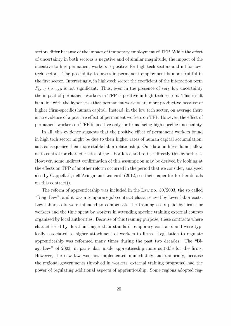
One of the most relevant determinants of sectoral uncertainty is technology (Krishnan

and Bhattacharya, 2002). If we look at the distribution of firm-specific uncertainty

at the beginning of the period by low and high tech sectors, identified according to

the standard OECD classification, we find that in Italy at the beginning of the past

decade the distribution of the firm-specific uncertainty is more skewed to the left for

high-tech sectors.11

Accordingly, we expect the effect of uncertainty on labor demand to be stronger in

high-tech sector; similarly, the effect of uncertainty and of the use temporary workers

on TFP should be even stronger. Table 9 reports the results of the regressions (13)-

(15) separately for high and low tech sectors. This exercise is not only interesting per

se but can also be viewed as a further robustness check.

The first 3 columns of Table 9 refer to labor demand equations. All the coefficients

have the same sign and magnitude than those reported on Table 4. However, the two

11For the purposes of this paper, we label hight (low) tech those firms belonging to the high(low) and medium-high (-low) OECD classification. High tech manufacturing sectors include NACE2-digit 24, 29, 30, 31, 32, 33, 34, and 35.

19

sectors differ because of the impact of temporary employment of TFP. While the effect

of uncertainty in both sectors is negative and of similar magnitude, the impact of the

incentive to hire permanent workers is positive for high-tech sectors and nil for low-

tech sectors. The possibility to invest in permanent employment is more fruitful in

the first sector. Interestingly, in high-tech sector the coefficient of the interaction term

Fi,r,s,t ∗ σi,r,s,0 is not significant. Thus, even in the presence of very low uncertainty

the impact of permanent workers in TFP is positive in high tech sectors. This result

is in line with the hypothesis that permanent workers are more productive because of

higher (firm-specific) human capital. Instead, in the low tech sector, on average there

is no evidence of a positive effect of permanent workers on TFP. However, the effect of

permanent workers on TFP is positive only for firms facing high specific uncertainty.

In all, this evidence suggests that the positive effect of permanent workers found

in high tech sector might be due to their higher rates of human capital accumulation,

as a consequence their more stable labor relationship. Our data on hires do not allow

us to control for characteristics of the labor force and to test directly this hypothesis.

However, some indirect confirmation of this assumption may be derived by looking at

the effects on TFP of another reform occurred in the period that we consider, analyzed

also by Cappellari, dell’Aringa and Leonardi (2012, see their paper for further details

on this contract)).

The reform of apprenticeship was included in the Law no. 30/2003, the so called

“Biagi Law”, and it was a temporary job contract characterized by lower labor costs.

Low labor costs were intended to compensate the training costs paid by firms for

workers and the time spent by workers in attending specific training external courses

organized by local authorities. Because of this training purpose, these contracts where

characterized by duration longer than standard temporary contracts and were typ-

ically associated to higher attachment of workers to firms. Legislation to regulate

apprenticeship was reformed many times during the past two decades. The “Bi-

agi Law” of 2003, in particular, made apprenticeship more suitable for the firms.

However, the new law was not implemented immediately and uniformly, because

the regional governments (involved in workers’ external training programs) had the

power of regulating additional aspects of apprenticeship. Some regions adopted reg-

20

ulations before others generating variation over space and time.12 Moreover the law

no. 80/2005 stated that in the absence of regional regulations, the introduction of the

“Biagi Law” should be regulated by sector-specific collective agreements, introducing

an additional source of variation.13

Cappellari, Dell’Aringa and Leonardi (2012) show that the reform of apprentice-

ship contracts induced the substitution of temporary workers with apprentices, with

positive effects on firms’ TFP. They argue that it follows from the training content of

the contract and from the longer duration which allow workers to accumulate human

capital. When discussing the results of Table 9 we argued that the direct positive

effect of permanent workers on TFP in the high-tech sector is probably due to the

possibility for permanent workers to invest in firm-specific human capital. If this

story holds true, we should find that also the introduction of apprenticeship, which

was directly aimed at increasing human capital, should have the same effect on TFP

of high-tech firms, regardless any indirect effect of uncertainty. Similarly, we should

find no effect of apprenticeship in low-tech industries, where the process of specific

human capital accumulation is likely to be less intensive.

We then define a dummy, labeled A equal to 1 for the years and sectors when

the apprenticeship reform took place. First, if we consider the full sample and we

do not split it by high and low tech sectors, we find that the overall average effect

of apprenticeship on TFP is around 3%. The size of this effect is fully comparable

with the finding of Cappellari, dell’Aringa and Leonardi (2012), who run a similar

regression. The results of the estimates by high and low tech firms are reported in

Table 10. Unfortunately, INVIND does not collect information about firms’ appren-

tices, and we cannot replicate the estimates presented in columns (1)-(4) of Table 9.

Thus, Table 10 refers then to TFP only. The effect of apprenticeship on TFP is very

high in high-tech firms (around 10 percentage points) and nil in low tech firms. In

the first sector, when controlling for uncertainty and for the interaction term A*σi,0,

the effect of apprenticeship survives and does not change its size, confirming that the

12These were Emilia-Romagna, Tuscany, Friuli-Venezia Giulia, Marche, Sardinia and the Au-tonomous province of Bolzano

13Between 2004 and 2007, collective agreements round involved Textile, Wood Products, Chemi-cals, Food Products and Metal Manufacturing. Between 2008 and 2010 all the other manufacturingsectors were involved.

21

positive effect on TFP is not due to the interaction between uncertainty and stan-

dard temporary positions, but is likely to be entirely due to this type of job contract,

which is associated with training activities. In low tech sectors the direct effect of

apprenticeship is not significantly different from zero while both the direct and the

indirect effects of uncertainty are statistically significant and have the expected sign.

8 Conclusions

The negative relationship between temporary work arrangements and labor produc-

tivity has been largely documented in the literature. However, a simple question

arises. Why do firms hire temporary workers then? Firms face is a clear trade off

between the optimal labor input choice and productivity levels. In this paper we tried

to show that there is an economic rationale behind hiring temporary workers, if they

are viewed as a of real option for firms: hiring permanent workers implies irreversible

costs mostly due to employment protection legislation, and when demand uncer-

tainty increases, firms may find convenient to postpone the decision to hire workers

permanently and exploit the current profit opportunities using less irreversible and

sometimes more costly (or less efficient) inputs of production, like temporary work.

We develop a dynamic model of labor demand with uncertainty that allows us to

draw some testable predictions on the level and on the composition of the labor force,

according to the level of uncertainty. The model suggests that when uncertainty in-

creases i) the number of permanent hirings decreases; ii) the number of temporary

hirings decreases, but seemingly less so with respect to permanent hirings; iii) the

number of total hirings decreases and iv) firms are prevented to adjust labor force to

demand conditions, therefore undermining their productivity level. An empirical test

of the aforementioned implications was performed based on data from the INVIND

survey, matched with balance sheet information from CADS. Our results indicate

that when uncertainty increases, total labor demand decreases, while the share of

temporary workers in total workforce grows. Therefore, uncertainty has in impact

both on the levels and on the composition of the workforce. Moreover, exploiting

an exogenous source of variation of workforce composition, we find that uncertainty

22

has a negative effect on productivity: the effect of the incentives to hire permanent

workers on TFP is stronger for firms who use temporary workers as substitute for

permanent positions as uncertainty increases.

23

References

Abel, Andrew B. and Eberly, Janice C. (1996) ‘Optimal Investment with Costly

Reversibility.’ Review of Economic Studies 63(4), 581–593

Acemoglu, Daron, and Jorn-Steffen Pischke (1999) ‘The Structure of Wages and In-

vestment in General Training.’ Journal of Political Economy 98(1), 426–438

Acharya, Viral V., Ramin P. Baghai, and Krishnamurthy V. Subramanian (2010)

‘Labor Laws and Innovation.’ NBER Working Papers

Angelini, Paolo, and Andrea Generale (2008) ‘On the Evolution of Firm Size Distri-

butions.’ American Economic Review 58(2), 277–297

Arellano, Manuel, and Stephen Bond (1991) ‘Some Tests of Specification for Panel

Data: Monte Carlo Evidence and an Application to Employment Equations.’

Review of Economic Studies 58(2), 277–297

Autor, David, William R. Kerr, and Adriana D. Kugler (2007) ‘Do Employment

Protections Reduce Productivity? Evidence from U.S. States.’ Economic Journal

117(521), 189–217

Bentolila, Samuel, and Giuseppe Bertola (1990) ‘Firing costs and labour demand:

How bad is eurosclerosis?’ Review of Economic Studies 57(3), 381–402

Bertola, Giuseppe, and Ricardo J. Caballero (1994) ‘Irreversibility and aggregate

investment.’ Review of Economic Studies 61(2), 223–246

Bird, Robert C. and Knopf, John D. (2009) ‘Do Wrongful-Discharge Laws Impair

Firm Performance?’ Journal of Law and Economics 52(2), 197–222

Bloom, Nick, Stephen Bond, and John van Reenen (2007) ‘Uncertainty and invest-

ment dynamics.’ The Review of Economic Studies 74(2), pp. 391–415

Boeri, Tito, and Pietro Garibaldi (2007) ‘Two Tier Reforms of Employment Protec-

tion: a Honeymoon Effect?’ Economic Journal 117(521), 357–385

Caggese, Andrea, and Vicente Cunat (2008) ‘Financing constraints and fixed term

employment contracts.’ Economic Journal 118(533), 2013–2046

24

Cappellari, Lorenzo, Carlo DellAringa, and Marco Leonardi (2012) ‘Temporary em-

ployment, job flows and productivity: a tale of two reforms.’ Economic Journal

122(4), 188–215

Chen, Yu-Fu, and Michael Funke (2009) ‘Threshold effects of dismissal protection

regulation and the emergence of temporary work agencies.’ Studies in Nonlinear

Dynamics and Econometrics 13(4), Article 3

Cipollone, Piero, and Anita Guelfi (2003) ‘Tax Credit Policy and Firms’ Behaviour:

the Case of Subsidy to Open-end Labour Contract in Italy.’ Temi di Discussione,

Bank of Italy

Dixit, Avinash (1989) ‘Entry and Exit Decisions under Uncertainty.’ Journal of Po-

litical Economy 97(3), 620–638

Dixit, Avinash, and Robert Pindyck (1994) Investment Under Uncertainty (Prince-

ton, New Jersey: Princeton University Press)

Dolado, Juan J., and Rodolfo Stucchi (2008) ‘Do temprary contracts affect tfp?

evidence from spanish manufacturing firms.’ CEPR Discussion Papers 7055,

C.E.P.R. Discussion Papers, November

Dolado, Juan J. Salvador Ortiguira, and Rodolfo Stucchi (2012) ‘Does Dual Em-

ployment Protection Affect TFP? Evidence from Spanish Manufacturing Firms.’

CEPR Discussion Papers n 8763

Foote, David A., and Timothy Folta (2002) ‘Temporary Workers as Real Options.’

Human Resource Management Review 12(4), 579–597

Guiso, Luigi, and Giuseppe Parigi (1999) ‘Investment and Demand Uncertainty.’

Quarterly Journal of Economics 114(1), 185–227

Krishnan, V., and Shantanu Bhattacharya (2002) ‘Technology selection and commit-

ment in new product development: The role of uncertainty and design flexibility.’

Management Science 48(3), 313–327

Levinsohn, James, and Amil Petrin (2003) ‘Estimating production functions using

inputs to control for unobservables.’ The Review of Economic Studies 70(2), 317–

341

25

Lucidi, Carlo (2006) ‘Is there a Trade-off between Labour Flexibility and Productivity

Growth? Preliminary Evidence from Italian Firms.’ mimeo

Luigi, Guiso, Luigi Pistaferri, and Fabiano Schivardi (forthcoming) ‘Credit within the

Firm.’ Review of Economic Studies

Michie, Jonathan, and Maura Sheehan (2003) ‘Labour Market Deregulation, ‘Flexi-

bility’ and Innovation.’ Canadian Journal of Economics 27(1), 123–143

Pindyck, Robert S. (1988) ‘Irreversible Investment, Capacity Choice, and the Value

of the Firm.’ American Economic Review 78(5), 969–985

Rodriguez-Gutierrez, Cesar (2006) ‘An Explanation of the Changes in the Proportion

of Temporary Workers in Spain.’ Applied Economics 38, 47–62

Saint-Paul, Gilles (1997) Dual Labour Markets: a Macroeconomic Perspective (Cam-

bridge, MA: MIT Press)

Wagner, Joachim. (1997) ‘Firm Size and Job Quality: A Survey of the Evidence from

Germany.’ Small Business Economics 9(5), 411–425

26

Table 1: Model’s parameters and their values for calibration.

Parameter Valueσlow 0.15σhigh 0.25η 0.00ρ 0.50wP 1.00wT 1.00ch 0.05cf 0.05bh 0.02bf 0.05λh 0.01λf 0.50A 1.00K 6.00

27

Table 2: Sample size, mean and standard deviation of the main variables.Observations Mean St. dev.

Firm uncertainty (σ) 10,804 0.081 0.077Total workforce percentage change 10,796 -0.003 0.096Permanent workers percentage change 10,740 -0.011 0.135Share temporary workers 10,804 0.094 0.245Temporary workers percentage change 10,402 -0.034 0.695Total factor productivity (log) 10,660 3.066 0.640

Notes: INVIND-CADS data. Firm uncertainty is equal to the squared of the differencebetween the upper and the lower bound of the real expected demand change in percentageterms, as stated by firms in 1999-2001. Total workforce percentage change is equal to thedifference between hires and separations between time t and t+ 1 and total workforce att. Permanent workers percentage change is defined as above but it refers only to flowsof permanent workers. The share of temporary workers is calculated with respect tototal workforce. TFP (in logs) is estimated according to the semi-parametric estimatordeveloped by Levinsohn and Petrin (2003, see Section 3 for details).

28

Table 3: Sample size by year.Year Observations1999 1,1062000 1,0812001 1,0442002 9882003 9352004 8732005 8592006 8262007 7892008 7642009 7082010 687Total 10,660

Notes: INVIND-CADS data by year. The sam-ple includes only firms participating to INVINDin 1999 or entering the sample in 2000-2001, forwhich a merge with CADS was possible.

29

Table 4: Worker composition and uncertainty.(1) (2) (3)

∆ total ∆ permanent Hires temporary w.workforce (%) workers (%) over total work.

σi,0 -0.041*** -0.043*** 0.057*[0.017] [0.017] [0.030]

Sector dummies yes yes yesTime dummies yes yes yesRegion dummies yes yes yes

Observations 10,772 10,744 10,804R-squared 0.05 0.04 0.32

Notes: In column (1) the dependent variable is the annual percentage change of totalworkforce. In column (2) the dependent variable is the annual percentage change of per-manent workers. In column (3) the dependent variable is the number of yearly hires oftemporary workers in total workforce. The fixed effect σi,0 is equal to the squared of thedifference between the upper and the lower bound for the real expected demand changein percentage terms, declared by firms in 1999-2001. Robust standard errors in brackets.* significant at 10%; ** significant at 5%; *** significant at 1%.

30

Table 5: Reforms and the growth rate of temporary and permanent employment.

(1) (2)∆ temporary ∆ permanentworkers (%) workers (%)

F -0.045* 0.022**[0.026] [0.010]

Time fixed effect yes yesSector fixed effects yes yesRegion fixed effects yes yesObservations 9,845 10,241R-squared 0.036 0.078

Notes: In column (1) the dependent variable is the annual growth rateof temporary workers. In columns (2) it is the annual growth rate ofpermanent workers. The variable F is a measure of fiscal incentivesto hire permanent workers. It is equal to 0 for the years of no fiscalincentive to the hires of permanent workers and equal to the fiscalincentive paid in the region of the main branch of firm, normalized bythe maximum incentive paid over the period 2001-2010. The estimatesinclude also time*region dummies. Robust standard errors in brackets.* significant at 10%; ** significant at 5%; *** significant at 1%.

31

Table 6: TFP, uncertainty and permanent employment. Standard errors in brackets.

(1) (2) (3) (4)TFP (log)

F 0.034* 0.034* 0.001[0.020] [0.020] [0.023]

σi,0 -0.499*** -0.500*** -0.652***[0.069] [0.069] [0.092]

σi,0*F 0.390**[0.150]

Sector dummies yes yes yes yesTime dummies yes yes yes yesRegion dummies yes yes yes yes

Observations 10,397 10,397 10,397 10,397R-squared 0.50 0.51 0.51 0.51

Notes: In all columns the dependent variable is the log of TFP, which is esti-mated according to the semi-parametric estimator developed by Levinsohn andPetrin (2003, see Section 3 for details). The fixed effect σi,0 is equal to thesquared of the difference between the upper and the lower bound for the realexpected demand change in percentage terms, declared by firms in the period1999-2001. The variable F is equal to 0 for the years of no fiscal incentive to thehires of permanent workers and equal to the fiscal incentive paid in the regionof the main branch of firm, normalized by the maximum incentive paid for theperiod 2001-2010. Robust standard errors in brackets. * significant at 10%; **significant at 5%; *** significant at 1%.

32

Table 7: Robustness checks: estimates for the sub-period 2006-2010.

(1) (2) (3) (4)∆ total ∆ permanent Hires temporary w. TFP

workforce (%) workers (%) over total work. (log)σi,0 -0.032* -0.050** 0.079** -0.572***

[0.019] [0.023] [0.040] [0.143]

Sector dummies yes yes yes yesTime dummies yes yes yes yesRegion dummies yes yes yes yesObservations 3,754 3,749 3,763 3,612R-squared 0.03 0.02 0.12 0.51

Notes: In column (1) the dependent variable is the annual percentage change of total workforce. Incolumn (2) the dependent variable is the annual percentage change of permanent workers. In column(3) the dependent variable is the number of yearly hires of temporary workers in total workforce.In column (4) the dependent variable is the log of TFP, which is estimated according to the semi-parametric estimator developed by Levinsohn and Petrin (2003, see Section 3 for details). The fixedeffect σi,0 is equal to the squared of the difference between the upper and the lower bound for the realexpected demand change in percentage terms, declared by firms in the period 1999-2001. Robuststandard errors in brackets. * significant at 10%; ** significant at 5%; *** significant at 1%.

33

Table 8: Unexpected demand change. IV estimates for the sub-period 2006-2010.Standard errors in brackets.

First-Stage Second stage(1) (2) (3) (4) (5)

Uncertainty ∆ total ∆ perm. Hires temp. TFPσi,0 work. (%) work. (%) over tot. (log)

Demand shock 0.383at t0 [0.027]***

σi,0 -0.187*** -0.304*** 0.116 -2.747***[0.089] [0.116] [0.203] [0.589]

Sector d. yes yes yes yes yesTime d. yes yes yes yes yesRegion d. yes yes yes yes yesObservations 2,722 2,708 2,710 2,710 2,655R-squared 0.24 0.04 0.01 0.11 0.50

Notes: The first column reports the first-stage. The σi,0 is equal to the squared of the differencebetween the upper and the lower bound for the real expected demand change in percentage terms,declared by firms in the period 1999-2001. The instrumental variable is the unexpected demandpercentage change equal to the difference between realized change observed in 1999 (or 2000, or2001, according to the time of entry into the panel) and the change that the firms stated to expectfor that year during the previous year interview. Columns (2)-(5) reports second-stage regressions.In column (2) the dependent variable is the difference between hires and fires between time t andt+1 and total workforce at t. In column (3) the dependent variable id defined as in (2), but it refersonly to flows of permanent workers. In column (4) the dependent variable is the share of temporaryworkers in total workforce. In column (5) the dependent variable (TFP) is estimated according tothe semi-parametric estimator developed by Levinsohn and Petrin (2003, see Section 3 for details).Robust standard errors in brackets. * significant at 10%; ** significant at 5%; *** significant at1%.

34

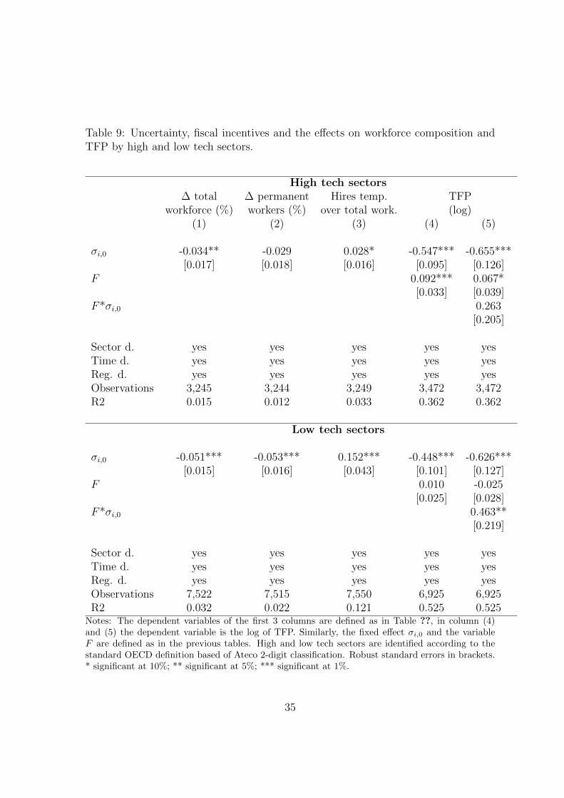
Table 9: Uncertainty, fiscal incentives and the effects on workforce composition andTFP by high and low tech sectors.

High tech sectors∆ total ∆ permanent Hires temp. TFP

workforce (%) workers (%) over total work. (log)(1) (2) (3) (4) (5)

σi,0 -0.034** -0.029 0.028* -0.547*** -0.655***[0.017] [0.018] [0.016] [0.095] [0.126]

F 0.092*** 0.067*[0.033] [0.039]

F*σi,0 0.263[0.205]

Sector d. yes yes yes yes yesTime d. yes yes yes yes yesReg. d. yes yes yes yes yesObservations 3,245 3,244 3,249 3,472 3,472R2 0.015 0.012 0.033 0.362 0.362

Low tech sectors

σi,0 -0.051*** -0.053*** 0.152*** -0.448*** -0.626***[0.015] [0.016] [0.043] [0.101] [0.127]

F 0.010 -0.025[0.025] [0.028]

F*σi,0 0.463**[0.219]

Sector d. yes yes yes yes yesTime d. yes yes yes yes yesReg. d. yes yes yes yes yesObservations 7,522 7,515 7,550 6,925 6,925R2 0.032 0.022 0.121 0.525 0.525

Notes: The dependent variables of the first 3 columns are defined as in Table ??, in column (4)and (5) the dependent variable is the log of TFP. Similarly, the fixed effect σi,0 and the variableF are defined as in the previous tables. High and low tech sectors are identified according to thestandard OECD definition based of Ateco 2-digit classification. Robust standard errors in brackets.* significant at 10%; ** significant at 5%; *** significant at 1%.

35

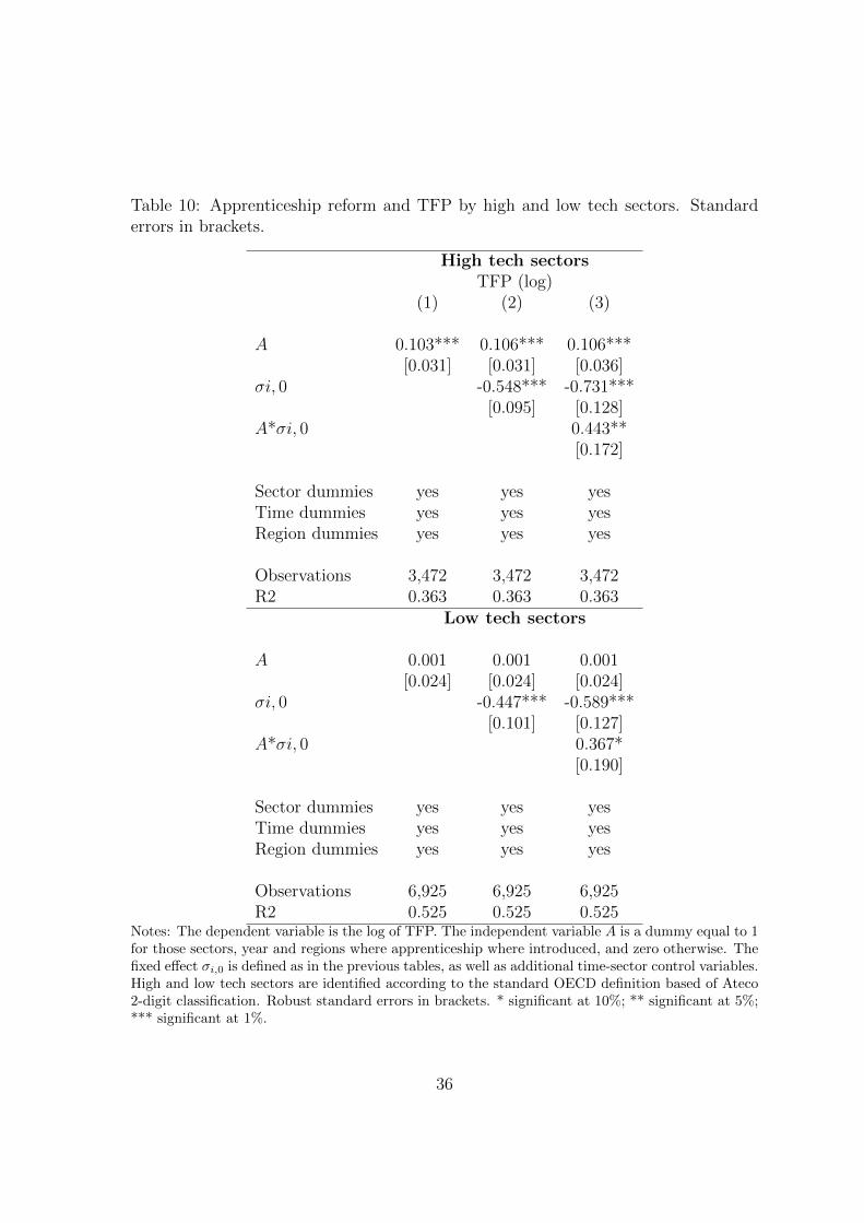
Table 10: Apprenticeship reform and TFP by high and low tech sectors. Standarderrors in brackets.

High tech sectorsTFP (log)

(1) (2) (3)

A 0.103*** 0.106*** 0.106***[0.031] [0.031] [0.036]

σi, 0 -0.548*** -0.731***[0.095] [0.128]

A*σi, 0 0.443**[0.172]

Sector dummies yes yes yesTime dummies yes yes yesRegion dummies yes yes yes

Observations 3,472 3,472 3,472R2 0.363 0.363 0.363

Low tech sectors

A 0.001 0.001 0.001[0.024] [0.024] [0.024]

σi, 0 -0.447*** -0.589***[0.101] [0.127]

A*σi, 0 0.367*[0.190]

Sector dummies yes yes yesTime dummies yes yes yesRegion dummies yes yes yes

Observations 6,925 6,925 6,925R2 0.525 0.525 0.525

Notes: The dependent variable is the log of TFP. The independent variable A is a dummy equal to 1for those sectors, year and regions where apprenticeship where introduced, and zero otherwise. Thefixed effect σi,0 is defined as in the previous tables, as well as additional time-sector control variables.High and low tech sectors are identified according to the standard OECD definition based of Ateco2-digit classification. Robust standard errors in brackets. * significant at 10%; ** significant at 5%;*** significant at 1%.

36

Fig

ure

1:In

acti

onzo

ne,

wit

han

dw

ithou

tte

mp

orar

yem

plo

ym

ent.

0510152025

113

2130

3948

5665

7483

9110

010

911

812

6

Em

plo

ymen

t

Inaction area

Inac

tion

zone

with

per

man

ent w

orke

rs o

nly

Inac

tion

zone

with

bot

h ki

nds

of w

orke

rs

2

5

5

0

7

5

100

125

37

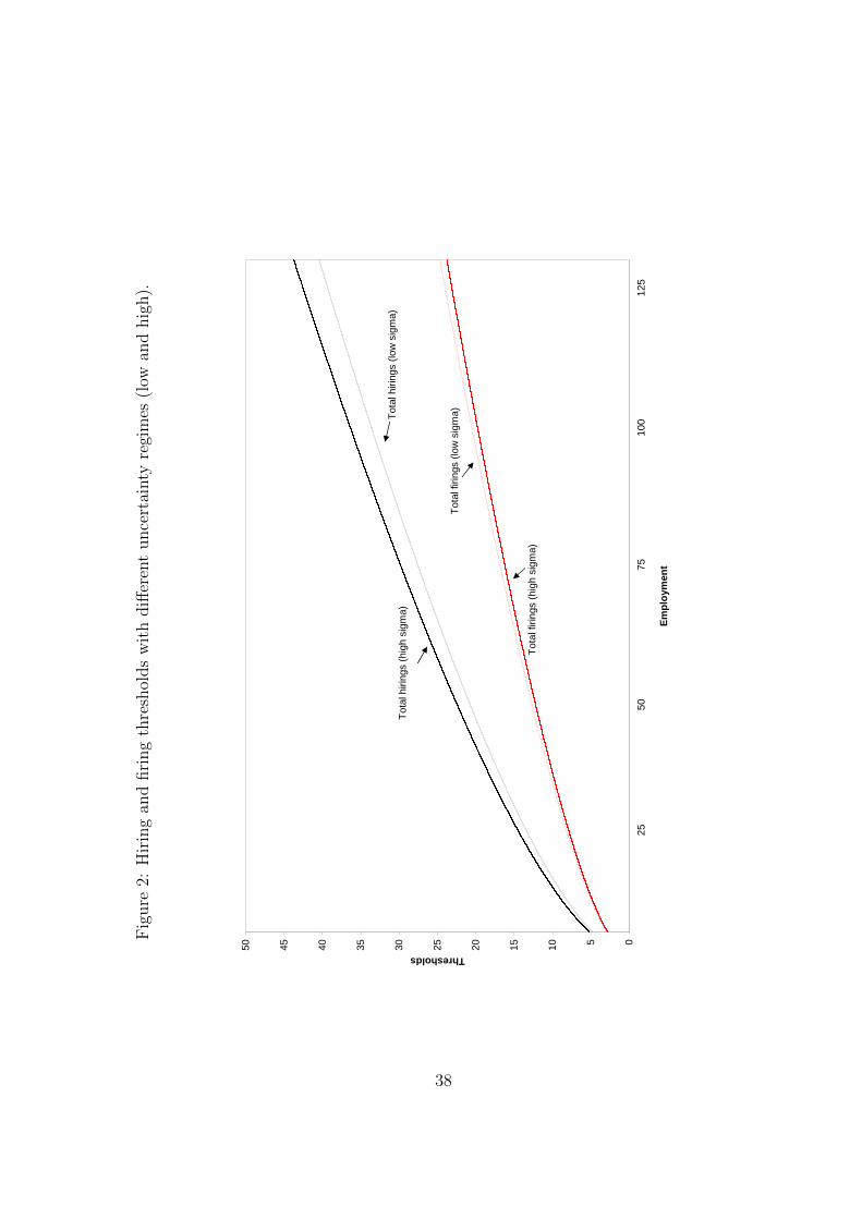
Fig

ure

2:H

irin

gan

dfiri

ng

thre

shol

ds

wit

hdiff

eren

tunce

rtai

nty

regi

mes

(low

and

hig

h).

05101520253035404550

4

7

10

13

17

20

23

26

29

32

36

39

42

45

48

51

54

58

61

64

67

70

73

76

80

83

86

89

92

95

99

102

105

108

111

114

117

121

124

127

Em

plo

ymen

t

Thresholds

2

5

5

0

7

5

100

125

Tot

al h

iring

s (lo

w s

igm

a)T

otal

hiri

ngs

(hig

h si

gma)

Tot

al fi

rings

(hi

gh s

igm

a)

Tot

al fi

rings

(lo

w s

igm

a)

38

Fig

ure

3:H

irin

gth

resh

olds

wit

hdiff

eren

tunce

rtai

nty

regi

mes

(low

and

hig

h),

for

tota

l,te

mp

orar

yan

dp

erm

anen

tem

plo

ym

ent.

05101520253035404550

4

7

11

14

18

21

24

28

31

35

38

41

45

48

52

55

58

62

65

69

72

75

79

82

86

89

92

96

99

103

106

109

113

116

120

123

126

Em

plo

ymen

t

Hiring threshold

1

25

50

75

100

1

25

Tem

pora

ry h

iring

s (lo

w s

igm

a)

Per

man

ent h

iring

s (lo

w s

igm

a)

Per

man

ent h

iring

s (h

igh

sigm

a)

Tem

pora

ry h

iring

s (h

igh

sigm

a)

Tot

al h

iring

s (h

igh

sigm

a)

Tot

al h

iring

s (lo

w s

igm

a)

39

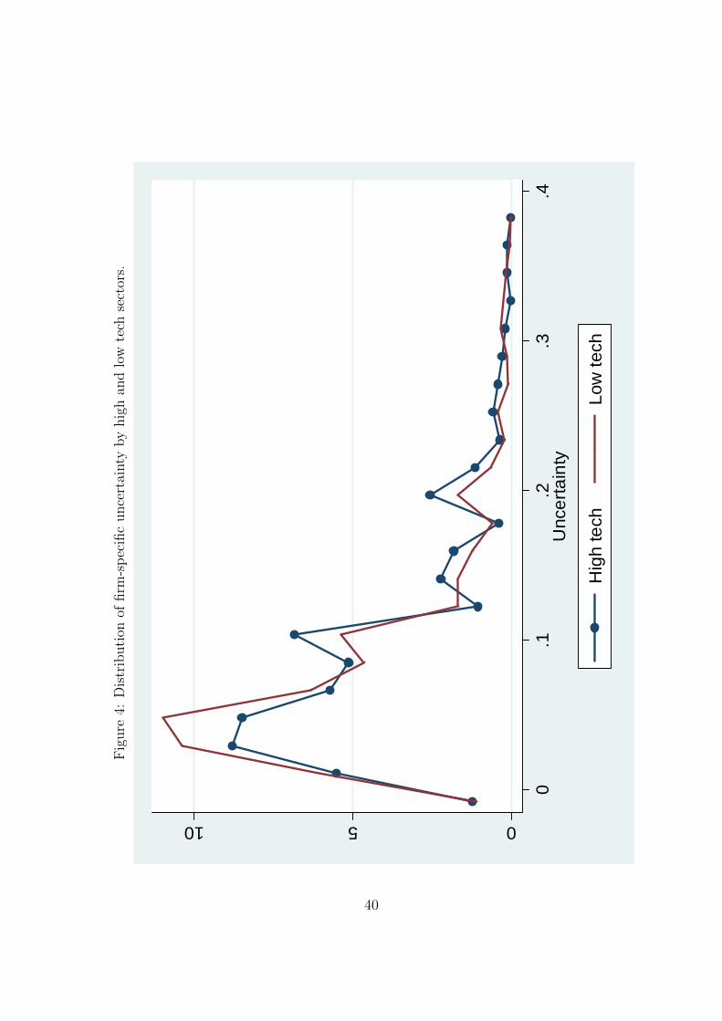
Fig

ure

4:D

istr

ibuti

onof

firm

-sp

ecifi

cunce

rtai

nty

by

hig

han

dlo

wte

chse

ctor

s.

0510

0.1

.2.3

.4U

ncer

tain

ty

Hig

h te

chLo

w te

ch

40