Embed Size (px)
Citation preview

Temporal analysis and scheduling of hard real-timeradios running on a multi-processorMoreira, O.
DOI:10.6100/IR724538
Published: 01/01/2012
Document VersionPublisher’s PDF, also known as Version of Record (includes final page, issue and volume numbers)
Please check the document version of this publication:
• A submitted manuscript is the author's version of the article upon submission and before peer-review. There can be important differencesbetween the submitted version and the official published version of record. People interested in the research are advised to contact theauthor for the final version of the publication, or visit the DOI to the publisher's website.• The final author version and the galley proof are versions of the publication after peer review.• The final published version features the final layout of the paper including the volume, issue and page numbers.
Link to publication
Citation for published version (APA):Moreira, O. (2012). Temporal analysis and scheduling of hard real-time radios running on a multi-processorEindhoven: Technische Universiteit Eindhoven DOI: 10.6100/IR724538
General rightsCopyright and moral rights for the publications made accessible in the public portal are retained by the authors and/or other copyright ownersand it is a condition of accessing publications that users recognise and abide by the legal requirements associated with these rights.
• Users may download and print one copy of any publication from the public portal for the purpose of private study or research. • You may not further distribute the material or use it for any profit-making activity or commercial gain • You may freely distribute the URL identifying the publication in the public portal ?
Take down policyIf you believe that this document breaches copyright please contact us providing details, and we will remove access to the work immediatelyand investigate your claim.
Download date: 13. Jun. 2018

Temporal Analysis and Scheduling of Hard
Real-Time Radios running on a Multi-Processor
Orlando Moreira

ISBN: 978-94-6191-140-7
The work described in this thesis has been carried out at Philips Re-search, NXP Research, and ST-Ericsson, as part of their respective R&Dprogrammes.
This work was supported in part by Agentschap NL (an agency ofthe Dutch Ministry of Economical Affairs), as part of the EUREKA/CA-TRENE/COBRA project under contract CA104.

Temporal Analysis and Scheduling of Hard Real-TimeRadios Running on a Multi-Processor
PROEFSCHRIFT
ter verkrijging van de graad van doctor aan deTechnische Universiteit Eindhoven, op gezag van de
rector magnificus, prod.dr.ir. C.J. van Duijn, voor eencommissie aangewezen door het College voor
Promoties in het openbaar te verdedigenop dinsdag 10 januari 2012 om 16.00 uur
door
Orlando Miguel Pires dos Reis Moreira
geboren te Porto, Portugal

Dit proefschrift is goedgekeurd door de promotoren:
prof.dr. H. Corporaalenprof.dr.ir. C.H. van Berkel
Copromotor:dr.ir. M.C.W. Geilen

Abstract
On a multi-radio baseband system, multiple independent transceivers mustshare the resources of a multi-processor, while meeting each its own hardreal-time requirements. Not all possible combinations of transceivers areknown at compile time, so a solution must be found that either allows forindependent timing analysis or relies on runtime timing analysis.
This thesis proposes a design flow and software architecture that meetsthese challenges, while enabling features such as independent transceivercompilation and dynamic loading, and taking into account other challengessuch as ease of programming, efficiency, and ease of validation.
We take data flow as the basic model of computation, as it fits the appli-cation domain, and several static variants (such as Single-Rate, Multi-Rateand Cyclo-Static) have been shown to possess strong analytical properties.Traditional temporal analysis of data flow can provide minimum throughputguarantees for a self-timed implementation of data flow. Since transceiversmay need to guarantee strictly periodic execution and meet latency require-ments, we extend the analysis techniques to show that we can enforce strictperiodicity for an actor in the graph; we also provide maximum latencyanalysis techniques for periodic, sporadic and bursty sources.
We propose a scheduling strategy and an automatic scheduling flow thatenable the simultaneous execution of multiple transceivers with hard-real-time requirements, described as Single-Rate Data Flow (SRDF) graphs.Each transceiver has its own execution rate and starts and stops indepen-dently from other transceivers, at times unknown at compile time, on amultiprocessor. We show how to combine scheduling and mapping decisionswith the input application data flow graph to generate a worst-case tempo-ral analysis graph. We propose algorithms to find a mapping per transceiverin the form of clusters of statically-ordered actors, and a budget for either aTime Division Multiplex (TDM) or Non-Preemptive Non-Blocking RoundRobin (NPNBRR) scheduler per cluster per transceiver. The budget is com-puted such that if the platform can provide it, then the desired minimum
v

vi
throughput and maximum latency of the transceiver are guaranteed, whileminimizing the required processing resources. We illustrate the use of thesetechniques to map a combination of WLAN and TDS-CDMA receivers ontoa prototype Software-Defined Radio platform.
The functionality of transceivers for standards with very dynamic be-havior – such as WLAN – cannot be conveniently modeled as an SRDFgraph, since SRDF is not capable of expressing variations of actor firingrules depending on the values of input data. Because of this, we proposea restricted, customized data flow model of computation, Mode-ControlledData Flow (MCDF), that can capture the data-value dependent behavior ofa transceiver, while allowing rigorous temporal analysis, and tight resourcebudgeting. We develop a number of analysis techniques to characterizethe temporal behavior of MCDF graphs, in terms of maximum latenciesand throughput. We also provide an extension to MCDF of our schedulingstrategy for SRDF. The capabilities of MCDF are then illustrated with aWLAN 802.11a receiver model.
Having computed budgets for each transceiver, we propose a way touse these budgets for run-time resource mapping and admissibility analysis.During run-time, at transceiver start time, the budget for each cluster ofstatically-ordered actors is allocated by a resource manager to platform re-sources. The resource manager enforces strict admission control, to restricttransceivers from interfering with each other’s worst-case temporal behav-iors. We propose algorithms adapted from Vector Bin-Packing to enable themapping at start time of transceivers to the multi-processor architecture,considering also the case where the processors are connected by a networkon chip with resource reservation guarantees, in which case we also findrouting and resource allocation on the network-on-chip. In our experiments,our resource allocation algorithms can keep 95% of the system resourcesoccupied, while suffering from an allocation failure rate of less than 5%.
An implementation of the framework was carried out on a prototypeboard. We present performance and memory utilization figures for thisimplementation, as they provide insights into the costs of adopting our ap-proach. It turns out that the scheduling and synchronization overhead foran unoptimized implementation with no hardware support for synchroniza-tion of the framework is 16.3% of the cycle budget for a WLAN receiveron an EVP processor at 320 MHz. However, this overhead is less than 1%for mobile standards such as TDS-CDMA or LTE, which have lower rates,and thus larger cycle budgets. Considering that clock speeds will increaseand that the synchronization primitives can be optimized to exploit theaddressing modes available in the EVP, these results are very promising.

Samenvatting
Op een basisbandsysteem van een smartphone met multi-radio onders-teuning delen meerdere gelijktijdig actieve, onafhankelijke radiozenders enontvangers onderdelen van de multi-processor hardware. Daarbij moet elkezender of ontvanger aan strenge real-time eisen voldoen. Omdat niet allecombinaties van zenders and ontvangers bekend zijn tijdens de ontwerp-fase, moet er een oplossing gevonden worden voor onafhankelijke analysevan temporele eigenschappen, dan wel moet die analyse in de smartphonezelf plaats vinden. Dit proefschrift beschrijft een ontwerpaanpak en soft-warearchitectuur die aan deze uitdagingen voldoen. Deze maken het mo-gelijk om diverse ontvangers en zenders onafhakelijk te compileren en dy-namisch te laden. Bovendien wordt voldaan aan eisen ten aanzien van pro-grammeerbaarheid, efficientie, en effectieve validatie. We kiezen dataflow alshet basis rekenmodel. Dataflow blijkt goed te passen bij het toepassingsge-bied (radioontangers/-zenders). Ook is van verschillende statische varianten,zoals enkelvoudig tempo (single rate), meervoudig tempo (multi-rate) en cy-clostatisch, bekend dat zij sterke analytische eigenschappen hebben. Tra-ditionele temporele analyse van dataflow kan garanties geven ten aanzienvan minimale gemiddelde doorvoersnelheid van een self-timed implementatievan dataflow. Omdat ontvangertaken vaak strict perodiek moeten wordenuitgevoerd en bovendien binnen een gegeven maximale wachttijd, breidenwe deze analysetechnieken hiertoe uit, zowel voor periodieke als voor on-regelmatige bronnen. Ook stellen wij een aanpak voor om de tijdsplanning(scheduling) te bepalen van de taken van meerdere gelijktijdig aktieve ra-dioontvangers met in achtname van de hard-real-time eisen. Elke ontvanger,beschreven als een dataflow graph, heeft hierbij een eigen tempo, en kanonafhakelijk van andere ontvangers gestart en gestopt worden op de multi-processor hardware. Wij laten zien hoe de tijdsplanning- en de afbeeldings-beslissingen kunnen worden gecombineerd, gebaseerd op de analyse van eenafgeleid dataflowmodel , onder veronderstelling van worst-case omstandighe-den. Daarnaast stellen wij algorithmen voor die voor elke ontvanger een
vii

viii
tijdsbudget vinden voor statisch geordende clusters van dataflowactoren.Daarnaast kunnen wij budgetten bepalen voor tijdgebaseerde multiplexing(TDM) en voor niet-onderbroken, niet-blokkerende Round Robin tijdsplan-ning per cluster, per ontvanger. Het budget wordt bepaald zodanig dat,mits de hardware hiertoe uigerust is, de gewenste minimale doorvoer enmaximale wachttijd kan worden gegarandeerd, en zodanig dat de hardwareminimaal wordt belast. Wij lichten een en ander toe aan de hand vaneen combinatie van WLAN en TDS-CDMA ontvangers op een prototypeSoftware Defined Radio platform. De functionaliteit van ontvangers metdynamisch gedrag, zoals WLAN, kan echter niet eenvoudig worden gemod-elleerd als een enkelvoudig-tempo dataflowgraaf, omdat in dergelijke grafende vuringsregels niet dataafhankelijk kunnen zijn. Daarom stellen wij eenaangepast dataflowmodel voor: Mode-Controlled Data Flow (MCDF), waar-bij een beperkte vorm van dataafhankelijk gedrag mogelijk is, en tegelijk-ertijd rigoreuze temporele analyse en budgetering mogelijk blijven. Hiertoeontwikkelen wij een aantal technieken om analyse van het temporele gedragvan dergelijke grafen mogelijk te maken, in termen van maximale wachtijdenen minimale doorvoer. Ook melden wij een uitbreiding van onze tijdsplan-ningaanpak naar MCDF, en illustreren wij dit aan de hand van een WLAN802.11a ontvangermodel. Wij stellen een aanpak voor om op basis van deuitgerekende tijdsbudgetten voor alle ontvangers hulpbronnen (resources)toe te wijzen en te bepalen of een ontvanger gestart kan worden. Tijdenshet gebruik (run time), wanneer een ontvanger gestart moet worden, wordtvoor elk cluster van statisch geordende actoren bepaald op welke hulpbron-nen die dient te worden uitgevoerd, zodanig dat verschillende ontvangerselkaar niet in de weg zitten. Algoritmen gebaseerd op vector bin-packingmaken het mogelijk om, na activering van de ontvanger, deze afbeelding opde multi-processor uit te voeren, inclusief routering en hulpmiddeltoewijz-ing op een network-on-chip. In onze experimenten kunnen tot 95% van dehulpmiddelen worden bezet, waarbij de afbeelding in minder dan 5% van degevallen mislukt.
De bovenstaande aanpak is uitgevoerd op prototype hardware. Wij pre-senteren de prestaties en benuttingsgraad van het geheugen van deze imple-mentatie, en verschaffen daarmee ook inzicht in de kosten van onze aanpak.Het blijkt dat de kosten van tijdsplanning en synchronizeren, zonder pro-cessorspecifieke optimalizaties en zonder specifieke hardwareondersteuningvoor synchronizatie 16.3% van het rekenbudget bedragen voor een WLANreceiver. Voor TDS-CDMA en LTE is deze overhead minder dan 1%, om-dat de synchronizatiefrequenties lager liggen. Gegeven de mogelijkheden totverdere optimalizaties beschouwen wij deze resultaten als veelbelovend.

Sumario
Num sistema de banda base multi-radio, multiplos receptores e transmis-sores independentes tem de partilhar os recursos de um multi-processador,ao passo que cada um deve ser executado em conformidade com os seusrequisitos de tempo-real estrito. Como nao sao conhecidas em tempo decompilacao todas as combinacoes possıveis de receptores e transmissoresque serao activadas durante a utilizacao do dispositivo, uma solucao deveser encontrada que seja capaz de permitir analise temporal independente decada aplicacao, ou que, por outra, consiga levar a cabo a analise temporalem tempo de execucao.
Esta tese propoe um metodo de programacao e uma arquitectura de soft-ware que respondem a estes desafios, permitem a compilacao independentede aplicacoes e o carregamento dinamico de codigo, e tomam em consid-eracao outros desafios, tais como a facilidade de programar a plataforma, aeficiencia da implementacao e a facilidade de validacao do sistema.
Escolhemos os grafos de fluxos de dados (“data flow graphs”) como basepara o nosso modelo de computacao, visto adequarem-se ao domınio deaplicacao, e tendo em conta que as suas variantes estaticas (“single-rate”,“multi-rate” e “cyclo-static”) exibem robustas propriedades analıticas. Astecnicas tradicionais de analise temporal de grafos de fluxos de dados po-dem fornecer garantias de taxa de transferencia mınima para execucao auto-temporizada. Visto que as aplicacoes de radio podem precisar de garantirexecucao estritamente periodica e garantir requisitos em termos de latencias,extendemos as tecnicas de analise temporal para mostrar que, em certascondicoes, podemos forcar periodicidade estrita na execucao de um actor naexecucao auto-temporizada do grafo de fluxo de dados, e propomos tecnicasde analise de maxima latencia para fontes periodicas, esporadicas e “bursty”.
Alem disso propomos uma estrategia e algoritmos de escalonamentoque permitem a execucao simultanea de varas aplicacoes com requisitosde tempo-real estrito, descritas enquanto grafos “Single Rate Data Flow”(SRDF). Cada aplicacao tem a sua propria taxa de transferencia de dados
ix

x
e comeca e acaba a execucao independentemente das outras, em momentosque nao sao conhecidos em tempo de compilacao, num multi-processador.Mostramos como combinar decisoes de escalonamento e mapeamento como grafo funcional da aplicacao para gerar um grafo que pode ser utilizadopara uma analise conservativa (“worst-case”) do comportamento temporalda aplicacao mapeada. Propomos algoritmos para encontrar um mapea-mento parcial para cada aplicacao atraves da criacao de agrupamentos deactores ordenados estaticamente, e da computacao de um orcamento de re-cursos que assume a utilizacao de um escalonador dinamico “Time DivisionMultiplex” (TDM) ou Round-Robin Nao-bloqueante e Nao-preemptivo paracada agrupamento.
Os orcamentos sao calculados de tal forma que, caso a plataforma sejacapaz de fornecer a quantidade de recursos estipulados pelo orcamento aaplicacao, entao serao garantidas a taxa de transferencia mınima e a latenciamaxima desejadas. Em paralelo, tentamos seleccionar os orcamentos comvista a minimizar a quantidade de recursos de computacao requeridos. Ilus-tramos a utilizacao destas tecnicas no mapeamento de uma combinacao dereceptores para WLAN e TDS-CDMA numa plataforma usada para a pro-totipagem de solucoes para Radio Definido por Software (Software DefinedRadio – SDR).
A funcionalidade de receptores e transmissores para normas de radio comcomportamento muito dinamico – como, por exemplo, WLAN – nao pode serconvenientemente modelada com grafos SRDF, visto que SRDF nao e capazde exprimir variacoes de regras de activacao de actores que dependam dosvalores dos dados recebidos. Por causa disso, propomos um modelo de com-putacao restrito e adaptado as necessidades do nosso domınio de aplicacao,que denominamos Fluxo de Dados com Controlo Modal, ou “Mode Con-trolled Data Flow” (MCDF), que pode capturar o comportamento depen-dente dos valores de dados de um transmissor ou receptor de radio, sal-vaguardando ao mesmo tempo a habilidade de levar a cabo uma analiserigorosa do comportamento temporal e a computacao de orcamentos de re-cursos computacionais. Desenvolvemos varias tecnicas de analise para carac-terizar o comportamento temporal dos grafos MCDF, em termos de latenciasmaximas e taxa de transferencia de dados mınima. Tambem fornecemos umaextensao para MCDF da nossa estrategia de escalonamento para SRDF.Ilustramos as capacidades de MCDF com um modelo de receptor de WLAN802.11a.
Tendo calculado os orcamentos de recursos por aplicacao, propomosuma forma de utilizar esses orcamentos para o mapeamento de recursose analise da admissibilidade das aplicacoes em tempo de execucao. Quando

xi
e necessario executar uma nova aplicacao, o orcamento para cada agrupa-mento de actores ordenados estaticamente que pertence a essa aplicacao emapeado por um gestor de recursos aos recursos existentes na plataforma.O gestor de recursos garante controle estrito na admissao de aplicacoes, paraimpedir novas aplicacoes de interferir com a realizacao do comportamentoconservativo em tempo-real de aplicacoes que ja estao a executar. Propomosalgoritmos adaptados de “Vector Bin-packing” para permitir o mapeamentode aplicacoes a arquitectura multiprocessador, considerando tambem o casoem que os processadores estao conectados por um “network on chip” comgarantias de reserva de recursos, para o qual fazemos encaminhamento emapeamento no “network on chip”. Nas experiencias que levamos a cabo,os nossos algoritmos de alocacao de recursos podem manter 95% dos recur-sos ocupados, sofrendo de uma percentagem de falhas em encontrar umaalocacao exequıvel em menos de 5% das tentativas.
Uma implementacao da nossa arquitectura de software foi levada a cabonuma plataforma de prototipagem. Apresentamos resultados em termos dedesempenho e utilizacao da memoria, visto que nos ajudam a compreender ocusto de adoptar a nossa solucao. Os custos acrescidos da nossa solucao emtermos de escalonamento dinamico e sincronizacao para uma implementacaoque nao dispoe de quaisquer optimizacoes do hardware para melhorar odesempenho da sincronizacao de tarefas e de 16.3% do orcamento de ciclosde execucao para um receptor de WLAN num processador EVP a 320 MHz.Contudo, os custos acrescidos sao menos de 1% para normas de comunicacaomoveis tais como TDS-CDMA ou LTE, que tem sımbolos de mais longaduracao, e portanto maiores orcamentos de ciclos de execucao por sımbolo.Considerando que as velocidades de relogio ainda vao aumentar e que asfuncoes primitivas de sincronizacao podem ser optimizadas para exploraros modos de enderecamento disponıveis no EVP, estes resultados sao muitoprometedores.

xii

Contents
1 Setting the Stage 11.1 Streaming Applications . . . . . . . . . . . . . . . . . . . . . 21.2 Real-Time Applications . . . . . . . . . . . . . . . . . . . . . 31.3 Software-Defined Radio . . . . . . . . . . . . . . . . . . . . . 51.4 Multi-standard Multi-channel Radio . . . . . . . . . . . . . . 61.5 Baseband Hardware Architectures . . . . . . . . . . . . . . . 71.6 Problem Statement . . . . . . . . . . . . . . . . . . . . . . . . 9
1.6.1 Determinism and Predictability . . . . . . . . . . . . . 101.6.2 Algorithm Specification and Temporal Behavior . . . . 121.6.3 Resource Sharing and Timing Behavior . . . . . . . . 16
1.7 Sketching an approach . . . . . . . . . . . . . . . . . . . . . . 201.8 Contributions . . . . . . . . . . . . . . . . . . . . . . . . . . . 221.9 Thesis organization . . . . . . . . . . . . . . . . . . . . . . . . 24
2 Software Framework 252.1 Terminology . . . . . . . . . . . . . . . . . . . . . . . . . . . . 252.2 Hardware Architecture . . . . . . . . . . . . . . . . . . . . . . 262.3 Requirements . . . . . . . . . . . . . . . . . . . . . . . . . . . 28
2.3.1 Addressing the Requirements . . . . . . . . . . . . . . 312.4 Model of Computation . . . . . . . . . . . . . . . . . . . . . . 312.5 Resource Management Options and Choices . . . . . . . . . . 33
2.5.1 Deciding when to decide . . . . . . . . . . . . . . . . . 332.5.2 Task Synchronization . . . . . . . . . . . . . . . . . . 362.5.3 Choice of Local Schedulers . . . . . . . . . . . . . . . 37
2.6 Proposed Solution Overview . . . . . . . . . . . . . . . . . . . 382.6.1 Operating system . . . . . . . . . . . . . . . . . . . . . 392.6.2 Programming and Mapping Flow . . . . . . . . . . . . 40
2.7 Programming Language . . . . . . . . . . . . . . . . . . . . . 402.8 Related Work . . . . . . . . . . . . . . . . . . . . . . . . . . . 43
xiii

xiv
2.9 Conclusions . . . . . . . . . . . . . . . . . . . . . . . . . . . . 44
3 Data Flow Computation Models 473.1 Graphs . . . . . . . . . . . . . . . . . . . . . . . . . . . . . . . 47
3.1.1 Paths and Cycles in a Graph . . . . . . . . . . . . . . 473.2 Multi-Rate Data Flow Graphs . . . . . . . . . . . . . . . . . . 483.3 Single Rate Data Flow . . . . . . . . . . . . . . . . . . . . . . 513.4 Integer Data Flow . . . . . . . . . . . . . . . . . . . . . . . . 533.5 Conclusion . . . . . . . . . . . . . . . . . . . . . . . . . . . . 58
4 Temporal Analysis 594.1 External Sources in Data Flow . . . . . . . . . . . . . . . . . 614.2 Schedules . . . . . . . . . . . . . . . . . . . . . . . . . . . . . 62
4.2.1 Notation . . . . . . . . . . . . . . . . . . . . . . . . . . 624.2.2 Admissible Schedules . . . . . . . . . . . . . . . . . . . 624.2.3 Self-Timed Schedules . . . . . . . . . . . . . . . . . . . 634.2.4 Static Periodic Schedules . . . . . . . . . . . . . . . . 644.2.5 Monotonicity . . . . . . . . . . . . . . . . . . . . . . . 664.2.6 Relation between the WCSTS and SPS . . . . . . . . 67
4.3 Linear Timing of Self-timed execution . . . . . . . . . . . . . 694.4 Dependence Distance . . . . . . . . . . . . . . . . . . . . . . . 704.5 Strict Periodicity on a Self-Timed Schedule . . . . . . . . . . 714.6 Latency Analysis . . . . . . . . . . . . . . . . . . . . . . . . . 75
4.6.1 Definition of Latency and Maximum Latency . . . . . 754.6.2 Maximum Latency from a Periodic Source . . . . . . . 764.6.3 Modeling Latency Constraints from a Periodic Source 774.6.4 Maximum Latency from a Sporadic Source . . . . . . 784.6.5 Maximum Latency from a Bursty Source . . . . . . . 81
4.7 Related Work . . . . . . . . . . . . . . . . . . . . . . . . . . . 824.8 Conclusion . . . . . . . . . . . . . . . . . . . . . . . . . . . . 83
5 Compile Time Scheduling 855.1 Scheduler Inputs . . . . . . . . . . . . . . . . . . . . . . . . . 87
5.1.1 Target Platform . . . . . . . . . . . . . . . . . . . . . 875.1.2 Task Graph . . . . . . . . . . . . . . . . . . . . . . . . 885.1.3 Timing requirements . . . . . . . . . . . . . . . . . . . 885.1.4 Additional Constraints . . . . . . . . . . . . . . . . . . 89
5.2 Scheduler Output . . . . . . . . . . . . . . . . . . . . . . . . . 905.3 Modeling Resource Allocation . . . . . . . . . . . . . . . . . . 90
5.3.1 Communication channels . . . . . . . . . . . . . . . . 90

xv
5.3.2 Buffer size restriction . . . . . . . . . . . . . . . . . . 915.3.3 Task Scheduling . . . . . . . . . . . . . . . . . . . . . 915.3.4 TDM Scheduling . . . . . . . . . . . . . . . . . . . . . 915.3.5 NPNBRR Scheduling . . . . . . . . . . . . . . . . . . 935.3.6 Static Order Scheduling . . . . . . . . . . . . . . . . . 935.3.7 Combining Static Order and TDM . . . . . . . . . . . 945.3.8 Mixing Static Order and NPNBRR scheduling . . . . 955.3.9 Temporal Analysis Model . . . . . . . . . . . . . . . . 965.3.10 Temporal Analysis Model for Partial Schedules . . . . 98
5.4 Why we combine CTS and RTS . . . . . . . . . . . . . . . . . 1005.5 The Scheduling Problem . . . . . . . . . . . . . . . . . . . . . 103
5.5.1 Optimization Criteria . . . . . . . . . . . . . . . . . . 1045.5.2 Phase decoupling . . . . . . . . . . . . . . . . . . . . . 1055.5.3 Determining Scheduler Settings . . . . . . . . . . . . . 1055.5.4 Finding Static Order Schedules . . . . . . . . . . . . . 1065.5.5 Finding the Slice Times . . . . . . . . . . . . . . . . . 1105.5.6 Buffer Sizing . . . . . . . . . . . . . . . . . . . . . . . 1155.5.7 Scheduling Multi-rate graphs . . . . . . . . . . . . . . 1155.5.8 Phase Ordering . . . . . . . . . . . . . . . . . . . . . . 117
5.6 Example . . . . . . . . . . . . . . . . . . . . . . . . . . . . . . 1185.7 Related Work . . . . . . . . . . . . . . . . . . . . . . . . . . . 1235.8 Conclusion . . . . . . . . . . . . . . . . . . . . . . . . . . . . 124
6 Mode-Controlled Data Flow 1276.1 Model Overview . . . . . . . . . . . . . . . . . . . . . . . . . 1296.2 MCDF Constructs . . . . . . . . . . . . . . . . . . . . . . . . 130
6.2.1 The Mode Controller . . . . . . . . . . . . . . . . . . . 1306.2.2 Data-dependent Actors . . . . . . . . . . . . . . . . . 1306.2.3 Mode Tunnel Conversion . . . . . . . . . . . . . . . . 132
6.3 MCDF Construction Rules . . . . . . . . . . . . . . . . . . . 1336.4 Radio Modeling in MCDF . . . . . . . . . . . . . . . . . . . . 136
6.4.1 Example Application: DVB-T receiver . . . . . . . . . 1366.4.2 Example Application: Wireless LAN receiver . . . . . 136
6.5 Properties . . . . . . . . . . . . . . . . . . . . . . . . . . . . . 1396.5.1 Notation . . . . . . . . . . . . . . . . . . . . . . . . . . 1396.5.2 Determinism . . . . . . . . . . . . . . . . . . . . . . . 1406.5.3 Linear Timing . . . . . . . . . . . . . . . . . . . . . . 1406.5.4 Iterative behavior and Deadlock Freedom . . . . . . . 1416.5.5 FIFO ordering, Firing and Iteration counts . . . . . . 143
6.6 Schedules and Temporal Analysis . . . . . . . . . . . . . . . . 144

xvi
6.6.1 Precedence constraints . . . . . . . . . . . . . . . . . . 1466.6.2 Self-Timed Execution . . . . . . . . . . . . . . . . . . 1476.6.3 SRDF bound . . . . . . . . . . . . . . . . . . . . . . . 1476.6.4 Mode-Sequence Specific Reference Schedule . . . . . . 1496.6.5 Temporal Analysis of Variable-length Mode Sequences 1536.6.6 Temporal Analysis Summary . . . . . . . . . . . . . . 154
6.7 Scheduling MCDF graphs . . . . . . . . . . . . . . . . . . . . 1556.7.1 Generating Quasi-Static-Order Schedules . . . . . . . 1566.7.2 Modeling Quasi-Static Order Schedules in MCDF . . . 1576.7.3 Determination of Run-Time Scheduler Settings . . . . 1626.7.4 Determination of Buffer Sizes . . . . . . . . . . . . . . 162
6.8 Scheduling Experiments . . . . . . . . . . . . . . . . . . . . . 1646.9 Multi-Rate MCDF . . . . . . . . . . . . . . . . . . . . . . . . 1656.10 Related Work . . . . . . . . . . . . . . . . . . . . . . . . . . . 1676.11 Conclusions . . . . . . . . . . . . . . . . . . . . . . . . . . . . 168
7 Resource Manager 1717.1 Related Work . . . . . . . . . . . . . . . . . . . . . . . . . . . 1727.2 System Architecture . . . . . . . . . . . . . . . . . . . . . . . 173
7.2.1 Hardware . . . . . . . . . . . . . . . . . . . . . . . . . 1737.2.2 Application . . . . . . . . . . . . . . . . . . . . . . . . 175
7.3 Resource Allocation . . . . . . . . . . . . . . . . . . . . . . . 1787.3.1 Motivating Example . . . . . . . . . . . . . . . . . . . 1787.3.2 PT Resource Provision . . . . . . . . . . . . . . . . . . 1787.3.3 Job Resource Requirements . . . . . . . . . . . . . . . 1797.3.4 Network Resource Provision . . . . . . . . . . . . . . . 180
7.4 Mapping Jobs . . . . . . . . . . . . . . . . . . . . . . . . . . . 1827.4.1 Clustering Strategies . . . . . . . . . . . . . . . . . . . 1847.4.2 Shuffled Input . . . . . . . . . . . . . . . . . . . . . . 1847.4.3 Virtual Tile Placement . . . . . . . . . . . . . . . . . . 1857.4.4 Bisection According to Kernighan-Lin . . . . . . . . . 186
7.5 Experiments and Results . . . . . . . . . . . . . . . . . . . . . 1887.5.1 Systems with one router . . . . . . . . . . . . . . . . . 1887.5.2 Systems with more than one router . . . . . . . . . . . 193
7.6 Conclusions . . . . . . . . . . . . . . . . . . . . . . . . . . . . 197
8 Demonstrator 1998.1 Streaming Framework: Sea-of-DSPs . . . . . . . . . . . . . . 1998.2 Resource Manager Implementation . . . . . . . . . . . . . . . 2018.3 Prototype Figures . . . . . . . . . . . . . . . . . . . . . . . . 202

xvii
8.3.1 Memory . . . . . . . . . . . . . . . . . . . . . . . . . . 2028.3.2 Performance of BB-RM . . . . . . . . . . . . . . . . . 2038.3.3 Scheduling Overhead . . . . . . . . . . . . . . . . . . . 2038.3.4 Multi-radio Operation . . . . . . . . . . . . . . . . . . 2038.3.5 Resource Fragmentation . . . . . . . . . . . . . . . . . 204
8.4 Conclusion . . . . . . . . . . . . . . . . . . . . . . . . . . . . 205
9 Conclusions and Further Work 207
Bibliography 215
Acknowledgements 225
List of Publications 229
Curriculum Vitae 233


Chapter 1
Setting the Stage
There was a time when the access to a computer was a luxury shared byfew. A single computing machine owned by an university or business wouldservice many users, each of which would carefully prepare the programs heor she wished to submit to the machine. After doing the submission, theuser would have to wait until the machine could find the time in its busyschedule to process that particular program, and deliver the desired results.
In less than half a century, we find ourselves in a completely differentsituation. Computers are everywhere. Many common day tasks, like with-drawing money, scheduling an appointment, reading the news or listeningto music are handled by computers. We are so used to computers takingcare of things for us that we would have severe problems handling our dailyroutine without them. Besides the conspicuous desktops and laptops, thereis a multitude of computers discretely operating inside special-purpose de-vices. These are the computers in cars, mobile phones, CD/DVD-players,navigation systems, personal digital assistants, and games consoles, to namebut a few. In technical circles, it is common to refer to computers includedin such devices as “embedded systems.”
Some of the most widespread computer systems in our time are thoseresiding in cellular phones. The most recent report from the InternationalTelecommunication Union [45], indicates that, in 2009, there were 67 mobilephone subscriptions per 100 inhabitants worldwide. The same report indi-cates that in developing countries this percentage has more than doubledsince 2005. This incredible level of popularity makes the mobile phone aprimary means for deploying new computer-based products and services tothe world population at large. Current high-end cellular phones are capableof much more than simple wireless voice communication, including function-
1

2 CHAPTER 1. SETTING THE STAGE
alities such as media playing, gaming, personal digital assistant, messaging,satellite navigation, and Internet browsing. However, all this extra function-ality still requires connectivity. In fact, a lot of the functionality of mostcomputing machines these days is somehow related with communications.This has to do with a new emerging trend referred to as “cloud computing”[48, 42], where computing resources are virtualized and provided as a ser-vice across a network to the user devices. If this trend is to gain traction,as it seems likely, the functionality of consumer devices will tend to becomeeven more dependent on how well they handle communication. For portabledevices, this communication must be wireless.
This thesis is about solving a design problem on an embedded com-puter system designed to handle wireless communications. The applicationdomain is commonly referred to as radio baseband processing. It is an appli-cation domain where solutions up to this point have mainly been designedfollowing a very focused constraint-driven approach, using mostly dedicatedhardware, but where the need for an increase in flexibility – the shift fromsingle-radio to multi-radio systems - leads to an increase in unknown factorsthat will require us to employ more software and adopt more optimality-driven techniques, while trying to preserve as much as possible the essentialcharacteristics of a constraint-driven design.
One of the main requirements of this application is with respect to itstiming behavior, and because of that, radio baseband processing is said to bea real-time application. Because of its iterative and data-centric structure,radio baseband processing is also a streaming application.
In the reminder of this chapter, we will define what a streaming applica-tion is, what a real-time application is, what is involved in radio basebandprocessing, and how it is implemented in hardware. We will then be able todefine the problem that this thesis addresses.
1.1 Streaming Applications
As in [90], we will define streaming application as an application thatoperates over a long (potentially infinite) sequence of input data items. Thedata items are fed to the application from some external source, and eachdata item is processed for a limited time before being discarded. The resultof the computation is a long (potentially infinite) sequence of output dataitems. Most streaming applications are built around signal-processing func-tions applied on the input data set with little if any control-flow betweenthem.

1.2. REAL-TIME APPLICATIONS 3
Besides software-defined radio, examples of streaming applications in-clude other communication protocols, radar tracking, audio and video de-coding, audio and video processing, cryptographic kernels, and network pro-cessing.
1.2 Real-Time Applications
Many embedded applications are Real-Time (RT) applications. This meansthat the correctness of the results produced by executing these applicationsdepends not only on the functional correctness of the values produced, butalso on the time at which these values are produced. Many computer appli-cations we see in our everyday life have RT requirements. To enumerate buta few, we can refer action computer games, video and audio players, GSMcellular phone transceivers, and controllers for DVD player drives.
The reader may wonder if it is not the case that any computer applica-tion is an RT application. As a counter-example, we may give a text editor.Although it is certainly annoying if it takes a long time to re-paginate adocument when the user, for example, changes the font type for the wholedocument, the obtained result – a re-paginated document – is still altogethercorrect and useful. Per opposition, a first-person shooter game that fails toproduce a certain number of frames per second is unplayable; a Wi-Fi mo-dem that fails to acknowledge packet reception to the base station withinthe time interval specified by the standard will cause the base station toretransmit the same packet over and over again, effectively making commu-nication impossible; a DVD lens focus controller that fails to compute intime the adjustments to the distance between the lens and the disk surfacecauses the DVD player drive to be incapable of reading the DVD.
RT applications are a heterogeneous bunch. Classifying an applicationas real-time is normally not enough. It tells us only that the time at whichresults are produced matters. But what type of timing requirements arethere? And how important is it that we meet them?
To put it simply, timing requirements come in two basic types: through-put and latency. If we have a throughput requirement, then the rate atwhich an iterative application produces results is important, but there maynot be any imposition on the time interval between the arrival of an inputand the production of a dependent output. If the requirement does prescribea minimum or maximum time between the arrival of an input data iten andproduction of a related output data item, then it is a latency requirement. Areceiver for television broadcast is a good example of an application with a
4 CHAPTER 1. SETTING THE STAGE
throughput requirement, but without a latency requirement. It is importantthat the images arrive at a certain rate, in such a way that the illusion ofmovement is kept for the viewer, at the right pace, but how much time ittakes for the image to travel from the broadcast source to the TV screen isnot so important (to an extent, as anybody who has experienced hearing theneighbors celebrate a goal before seeing it ’live’ on her TV set may attestto). A networked multi-player first-person shooter game is a good exampleof an application with a latency requirement: the actions of each playermust affect the game world in such a way as to seem almost instantaneousto all players.
Temporal requirements can be in the form of a required worst-case tim-ing, a required best-case timing, or both. Sometimes, the worst-case and thebest case timing requirements coincide. This is sometimes referred to as anon-time requirement. We will not discuss on-time requirements or best casetiming requirements on this thesis. We will assume that it is always possibleto delay an output event, if that is necessary. In the general case, an RTapplication can come with several throughput and latency requirements.
Another important classification of RT applications is related with howstrict the timing requirement is. There are several classifications of RTapplications according to the strictness of the timing requirements. One ofthe simplest, and still very useful, divides RT applications into two types:soft real-time and hard real-time. Hard real-time applications are thosewhere requirements cannot be infringed under any circumstances, or theresults of the computation will be completely useless, and failure may, in thecase of a life critical system, have catastrophic consequences. In soft real-time applications, timing requirements can be occasionally disrespected, butthe rate of failures must be kept below a certain maximum.
There is also a class of applications where failing to meet the temporalrequirements may imperil lives. Such applications are often referred to ascritical RT applications. Some authors [52, 12] will only consider hard RTapplications the ones that are critical, and prefer to refer to other applica-tions with strict requirements as firm RT. From the experience of the authorof this thesis, the latter term is rarely if ever used in industrial settings.
It is important to keep in mind that the classification of a particularapplication may be in itself a choice that the designer must make. It is achoice where the trade-off is between the delivered quality and the cost ofthe solution. For instance, because human perception is relatively tolerantof frame loss in a video signal, and since there is a wide variation betweenthe average case and the worst case computational load, it is common totreat video decoding as a soft real-time application, whereas audio decoders,

1.3. SOFTWARE-DEFINED RADIO 5
since the variation of computational load is much lower and the effects oflosing a sample very noticeable by the user, are more frequently treated ashard RT applications.
1.3 Software-Defined Radio
Software-Defined Radio (SDR) is a streaming application domain where RTbehavior is often crucial. The term Software-Defined Radio was used for thefirst time by Joseph Mitola in 1992 [68]. The idea of SDR is that of relying onprogrammable processors to implement, by means of software programming,some of the stages of the processing involved in the reception/transmissionof a stream of wireless messages, modulated and coded according to a givenradio transmission protocol.
Independently of the particular protocol being implemented, digital radiotransceivers have a similar flow of data through a number of basic functionalblocks, as depicted in Figure 1.1. They are typically implemented in anumber of stages, which include:
• Radio-frequency filtering and conditioning stage, normally done in theanalogue domain;
• Conversion stage, where the analogue signal is sampled and quantizedto a digital signal (in the case of the receiver) or converted from digitalto analogue (in the case of the transmitter);
• Baseband processing stage, where the digital signal is (de)modulatedand (de)coded;
• Application layer, which may include higher layer communication pro-tocols (eg: a TCP/IP layer on a WLAN), or simple direct use of theraw received data for some user application, such as voice communi-cation.
In this thesis, we are interested in software-defined implementations ofthe real-time baseband processing stage of digital radio transceivers. Thebaseband processing stage of a digital radio is completely done in the digitaldomain. It has strict temporal constraints that imply its treatment as a hardRT application. However, in particular cases, such as Wireless LAN, we willassume that our concern extends to higher level protocols, as these constitutejointly with the baseband a single chain of functional dependencies overwhich a strict end-to-end real-time requirement is defined.

6 CHAPTER 1. SETTING THE STAGE
Vector Processing for Software-Defined Radio 2615
Table 1: Layers of a future seamless network.
Layer Link range (log10 m) Up/down Mobility Standards (examples)
Positioning 6-7 d Full GPS, GalileoDistribution 5-6 d Full DAB, DVB-T/HCellular/2G 4-5 d,u Full GSM, IS95, PHSCellular/3G 3-4 d,u Full UMTS, CDMA2000, TD-SCDMAHot-spot 2-3 d,u Local 802.11 a,b,g, wifiPersonal 1-2 d,u Local Bluetooth, DECTFixed 0-1 d,u None POTS
802.11a
UMTS
GSM
DVB-T
GPS
Load estimates (GHz)
11n(MIMO)
HSDPA, MIMO
EDGE, GPRS
Dopplercompensation
Galileo
0.1 0.3 1 3 10 30
Figure 2: Load estimates for various SDR standards.
of acceptable e!ciency for some algorithms, we rely on man-ual vectorization for the time being. Vectorization of severalkey algorithms is presented below. In the sequel we assumea vector processor that supports P (P a power of 2) identi-cal operations to be executed in parallel (single-instructionmultiple-data (SIMD)), as well as load (store) operations ofP adjacent values from (into) a vector memory.
3.1. Golay correlator for UMTS-FDD
In a UMTS-FDD receiver, a Golay correlator is used for initialacquisition of a basestation signal. It is basically a filter (1)designed specifically to detect correlation peaks of the 256-chip long primary synchronization code (PSC [3]) transmit-ted during the first 10% of each timeslot on the primary syn-chronization subchannel (P-SCH) [4]:
y(k) =255!
n=0
PSC(255! n)" x(k ! n) (1)
with PSC(i) # !1, +1 and x is one of the sample phasesof the over-sampled input stream of complex (I,Q) numbers.The structure of PSC(i) allows a factorization of the Golaycorrelator into five stages, as shown in (2). The alternativeoutput stage y$(k) is used only during initial frequency o"setestimation.
Input x, output y, and intermediate signals ys can bestored in cyclic bu"ers of appropriate sizes. With sharing of
ControlR
F/IF
D/A
A/D
Filte
rs
Mod
em
Cod
ec,(
de)m
ux
App
licat
ion
proc
essi
ng
Digital baseband
Figure 3: A crude SDR architecture with the baseband section splitinto filters, modem, and channel codec.
subexpressions, each output y(k) requires 13 complex addi-tions/subtractions, 14 memory reads, and 14 memory writes(of complex values). In principle, these operations can be ex-ecuted in parallel. However, as all operands reside in di"erentlocations of the various bu"ers, the resulting parallel accessesto memory become highly irregular, incompatible with vec-tor processing:
y1(k) = x(k ! 6) + x(k ! 4) + x(k ! 2)! x(k),
y2U(k) = y1(k ! 1) + y1(k),
y2L(k) = y1(k ! 1)! y1(k),
y3(k) = y2U(k ! 8) + y2L(k),
y4U(k) = y3(k ! 48) + y3(k ! 32) + y3(k ! 16)! y3(k),
y4L(k) = y3(k ! 48)! y3(k ! 32) + y3(k ! 16) + y3(k),
y(k) = y4U(k ! 192)! y4L(k ! 128)
+ y4U(k ! 64) + y4L(k),
y$(k) =""y4U(k ! 192)
""2 !""y4L(k ! 128)
""2
+""y4U(k ! 64)
""2 +""y4L(k)
""2.
(2)
Vectorization of the Golay correlator becomes rela-tively straightforward when P successive output symbolsy(k), y(k + 1), . . . , y(k + P ! 1) are computed in parallel.The resulting program follows the sequence of stages of (2),
Figure 1.1: The stages of a radio transceiver (adapted from a table providedby NXP Semiconductors).
1.4 Multi-standard Multi-channel Radio
In many devices, there is a huge variety of radio standards that need to besupported. This is both because different standards are developed to handledifferent types of data transfers, such as audio and video broadcast, two-way telephony, two-way data-link, navigation, and because for each typeof communication link there may be several different standards either dueto their different technical merits (range, data rate, latency, vulnerabilityto noise, etc) or political and intellectual property-related issues. Differ-ent standards are also used for different categories of devices. There are 3main market segments for this type of technology: mobile phones, cars, anddomestic appliances (home). Table 1.1 gives an overview of standards bymarket segment and application.
Without an SDR solution, handset makers build their systems by includ-ing a dedicated solution for each of the standards they wish to support. Thismakes the devices inflexible, and does not allow for post-design updates ofthe functionality.
Modern smartphones must not only support multiple standards, butmust also allow for multiple standards to be simultaneously active on a sin-gle mobile handset. To illustrate this point, consider an use-case: a hikerusing her mobile phone to listen to a digital radio station, via a cordlessBluetooth headset, at the same time using GPS to keep track of her po-sition for posterior plotting of her itinerary, while in the background herphone keeps listening to the cellular network for incoming calls, and an

1.5. BASEBAND HARDWARE ARCHITECTURES 7
Type Mobile Car Home
Positioning GPS, Gallileo GPS, Gallileo
BroadcastFM, DAB, DVB-T,DVB-H, STiMi
AM, FM, DAB,ISDB-T,ATSC, DVB-C, DVB-T, DVB-HT2,DMB-T
AM, FM, DAB, T-DMB, DRM, XM, Sir-ius, ISDB-T, DVB-T, DVB-H, HD-Radio,SDARS
Cellular: 3G+
UMTS, HSDPA,HSUPA, MBMS,LTE, TDS-CDMA,CDMA2000, LTEAdvance
Cellular: 2G+GSM, IS95, IS136,PHS, EDGE, GPRS
WLAN:802.11a, 802.11b,802.11g, 802.11n,WiMax
802.11a, 802.11b,802.11g, 802.11n,WiMax
802.11a, 802.11b,802.11g, 802.11n
WPAN Bluetooth, UWB, NFCDECT, Bluetooth,UWB, Zigbee
Bluetooth
Table 1.1: Profusion of Radio Standards
email client periodically checks for incoming emails. This is hardly a far-fetched example, and it requires at least 4 independent radio systems to beactive simultaneously.
1.5 Baseband Hardware Architectures
Different types of programs have different patterns of control flow and datamanipulation. A filter function, for instance, is typically computed by sum-ming up the results of multiplying 1-to-1 the elements of two long vectorsof numeric values; a decoder, on the other hand, normally involves manybit manipulation operations; a finite-state machine may be dominated byjumps in the program’s control flow caused by testing the values resultingfrom relatively simple arithmetical operations. By designing a processor toexcel at one specific type of function, one can achieve better performance,at lower area and power cost. This has led to the development of highlyheterogeneous computation platforms, with a set of different programmablecores optimized to handle domain-specific tasks, combined with Application-Specific Integrated Circuits (ASIC) accelerators designed to dramaticallyspeed-up a small set of application-specific functions.
Embedded multiprocessors are not strictly heterogeneous: it often makessense to employ several cores of the same type. This is done to exploit

8 CHAPTER 1. SETTING THE STAGE
thread-level parallelism and allow for higher computational capability thanwould be allowed in a power-efficient manner by increasing the clock speedof a single core (this assuming that an increase in clock speed is possible).
In the case of baseband processing, both academia and industry haveindependently proposed hardware platforms that follow the general trendof combining homogeneous and heterogeneous multiprocessing, employingmultiple vector processors, general-purpose processors and hardware accel-erators.
As described in [8], the baseband processing stage can be further splitinto three sub-stages: Digital Filtering, MoDem, and CoDec. These 3 sub-stages have very different computational characteristics. The Digital Fil-tering stage has very high computational load (up to 5 billion operationsper second for UMTS), and since the algorithms involved change little fromstandard to standard, full programmability is not required, and a simpleconfigurable filter is sufficient. The MoDem stage (often referred to as the“inner receiver”) is the most diverse among standards. Algorithms in thisstage often include heavy processing of vectors and matrix operations. Thisis typically implemented by means of a vector processor such as the EVP[8], capable of handling multiply-accumulate operations on many input val-ues simultaneously. The CoDec stage (also known as the “outer receiver”)is more oriented towards manipulation of bits and ordering of data, and,because there is less variety in algorithmic implementation, it is typicallyhandled by a number of ASIC accelerators. The flow control decisions takenby the application are typically handled by general-purpose cores, such asthe ones from the ubiquous ARM processor family.
One example of a system architecture for baseband-processing is the Mu-SIC software-defined baseband chip from Infineon [80], depicted in Figure1.2. This platform includes 4 digital signal processors – Single-InstructionMultiple Data (SIMD) cores, which handle vector operations, a programmableprocessor, two programmable accelerators, one dedicated to Turbo/Viterbi(de)coding and the other to FIR Filtering, and an array of RF interfaces.Each processor has its own dedicated memory, and a common memory isprovided for communication between the cores. The common memory ismulti-banked, thus allowing simultaneous accesses from the various bus mas-ters through a multi-layer bus.
Another architecture proposed for SDR is the SODA architecture [60]from the University of Michigan. It has many similarities with MuSIC. Ithas recently been redesigned as a commercial ARM Ltd prototype, calledScotch [94]. Both are depicted in Figure 1.3. As MuSIC, SODA employsfour SIMD cores, marked as PEs (Processing Elements) in the figure, each

1.6. PROBLEM STATEMENT 9
tocol stack software. External memories provide the codeand data storage. A couple of RF interfaces connect thebaseband processor to the digital front ends and provide
66 Computer
for filtering operations as well as channel encoding anddecoding. A general-purpose processor along with a setof standard peripherals executes the L1 control and pro-
Baseband processor
Seria
l I/F
Mul
tilay
er b
us
DSP 1
DSP n
Accelerators
...
PeripheralsSeria
l I/F
Seria
l I/F
Data 1
Data 2
Control
ClockAFE
AFE
Ampl./switch
Seria
l I/F
Data 1
Data 2
Control
ClockAFE
AFE
Ampl./switch
Mem
GSM/GPRS/EDGE, WCDMA, HSDPA, GPS
DFE
DFE
DFE
DFE
AP I/F Applicationprocessor
802.11a/b/g, WiMax, DVB-H,…, BT
Optional
SIMDcore 140 K
memory
SIMDcore 4
SIMD core cluster
RFinterfaces
AcceleratorTurbo/Viterbi
decoder
Externalmemory I/F
(Flash/DRAM)
GP coreprotocol
stack
I&D cache
Busbridge
Peripherals
Multilayer bus
Accelerator
FIR filter
SIMDcore 2
SIMDcore 3
Shared memory
128 K 128 K 128 K 128 K
PE 1
Communication network
L/S unit, DMA channels
Memory slot
DSPpipe
Intg. unit
Memory slot
DSPpipe
Intg. unit
PE 4
I-fetchand
decode
System bus
MultitaskedGP core
Local memoryLocal memoryI cache
RegistersRegisters
I&D cache
(a)
(b)
(c)
40 Kmemory
40 Kmemory
40 Kmemory
AFE: Analog front endDFE: Digital front end
PE: Processing element
Figure 3. Infineon’s MuSIC-1 chip. (a) Block diagram of SDR modem. (b) Baseband DSP. (c) SIMD core.
Authorized licensed use limited to: ST Microelectronics. Downloaded on March 2, 2009 at 05:05 from IEEE Xplore. Restrictions apply.
Figure 1.2: The MuSIC architecture, an SDR solution from Infineon (picturetaken from [80]).
with its own local memory, and a control processor. The Scotch prototypeintroduces changes to the communication and memory hierarchy, includinga DMA to handle data transfers between the background memory and thelocal memories, and hardware acceleration for Turbo decoding.
!"#$%&'
()*+
,-./
0&1-
2
3
!"#$%&'
()*+4
5678
*91'
()*+
(:9;;1-
<-'$
=>?@4
A((<B
C
D
(EF1F?4
567
C
D
2
3
(EF1F?
,0
6"
()*+
+F'F
*-G>?H
6"
(EF1F?
+F'F
*-G>?H
(
I
J
5K7
,02
3
C
D
5K7
567
"/4=&L-4()*+
#/4(EF1F?
M/45K7
J
I
(
N?-L/
,-.O
C
D
()*+
'>
(EF1F?
AJ'>(B
567
,0
+*5
(P+54N24
!/4+*5
Q/46>EF14
G-G>?H
(P+54(HO'-G4
I>4
(HO'-G4
D9O
!"#$%&'
()*+
,-./
0&1-
!"#$%&'
()*+4
*91'
()*+
(:9;;1-
<-'$
=>?@4
(EF1F?4
5678
*91'
(EF1F?
,085RR
6"
+F'F
*-G>?H
5K7
,0
5K7
"/4=&L-4()*+
N?-L/
,0
()*+8
(EF1F?
I?FSO;4
7S&'
5?L%-.4N24
Q/4*-G>?H
()*+
N?-L/
567
(EF1F?
=LF'F
"T#M$%&'
()*+4
5RR4,0
()*+
=LF'F4
!"#$%&'
()*+4
567
=&':
O:9;;1-
2
3
2
3
)
<
I
2
,
R
P
<
<
2
R
I
(
)
<
I
2
,
R
P
<
<
2
R
I
(
6#
*-G>?H
#/4(EF1F?4U45K76"
N?>.?FG
*-G>?H
R>S'?>11-?
)S'-?E>SS-E'4D9O
6#4
(E?F'E:VFL4
*-G>?H
R>S'?>1
N?>E-OO>?
6"
*-G>?&-O
2W-E9'&>S
7S&'
N24
6"
*-G>?&-O
2W-E9'&>S
7S&'
N24
6"
*-G>?&-O
2W-E9'&>S
7S&'
N24
6"
*-G>?&-O
2W-E9'&>S
7S&'
N24
XM$%&'45*D54Q453)4)S'-?E>SS-E'
I9?%>4
R>V?>E-OO>?+*5RN-?&V:-?F1O
6"
*-G
R>S'?>14
N?>E-OO>?
6"
*-G2W-E9'&>S
7S&'
N24
6"
*-G2W-E9'&>S
7S&'
N24
6#
*-G
!"#$%&'4444444D9O
2
3
2
3
5K7
5K7
5?L%-.4(HO'-G4
(P+5 5?L%-.
()*+484OEF1F?4845K7 ()*+484OEF1F?4845K7
()*+Y(EF1F?46)C ()*+Y(EF1F?4FSL4()*+Y()*+46)C
MTT*Z[4A"\TSGB Q!T*Z[4A]TSGB
N245?E:&'-E'9?-
O&S.1-4&OO9- 567484G-G>?H484((<
!"#4%&'O !"#4%&'O
"X$%&'403N \Y"XYQ#$%&'403N
()*+45?E:&'-E'9?-
S> H-O
H-O H-O
#4EHE1-O "4EHE1-
Q#$1FS-4"$O'F.-4&'-?F'&^-4V-?;-E'4O:9;;1- "#\$1FS-4_$O'F.-4DFSHFS4S-'=>?@
?-L9E'&>S4'?-- VF&?$=&O-4>V-?F'&>SY?-L9E'&>S4'?--
#4?-FLY"4=?&'-4V>?'O`4"X4-S'?&-O Q4?-FLY#4=?&'-4V>?'O`4"!4-S'?&-O
\aD Q#aDb"#\aD
XMaD #!XaDb"*D
S> I9?%>4E>V?>E-OO>?
S> O>;'=F?-4V&V-1&S&S.
P':-?O
P?.FS&[F'&>S
2W-E9'&>S4*>L-1
N240?-c9-SEH
()*+4+F'FVF':
()*+4C&L':
+F'F4N?-E&O&>S
D1>E@401>F'&S.4N>&S'
()*+4N?-L&EF'&>S
()*+4*91'46F'-SEH
()*+4(:9;;1-4<-'=>?@
,-L9E'&>S4<-'=>?@
()*+4,-.40&1-
6"4*-G>?H
6#4*-G>?H
R>V?>E-OO>?
R>GV&1-?4PV'&/
R>GVF?&O>S4O9GGF?H4>;4':-4F?E:&'-E'9?F14;-F'9?-O4>;4(P+54FSL45?L%-.
6"
N?>.?FG
*-G>?H
R>S'?>11-?
C
D
C
D
C
D
C
D
2
3
Figure 1: SODA and Ardbeg architectural diagrams, and a summary of the key architectural features of the two designs.
erator dedicated to Turbo decoding. In comparison, in theSODA system, Turbo decoding is allocated to one of thefour PEs. Both the Ardbeg and SODA PEs have three majorfunctional blocks: SIMD, scalar, and AGU.
The SODA and Ardbeg PEs both support 512-bit SIMDoperations. The SODA PE only supports 16-bit fixed point
operations, whereas the Ardbeg PE also supports 8-, 32-bitfixed point, as well as 16-bit block floating point operations.Support for 8-bit helped lower the power for many of theW-CDMA kernels that only needed 8-bit precision. Legacywireless protocols like 802.11b have many kernels thatoperate on 8-bit data and do not require the 16-bit precision
Figure 1.3: The SODA architecture, an SDR solution from the Universityof Michigan, and the Scotch prototype (picture taken from [94]).
1.6 Problem Statement
The MuSIC and SODA hardware architectures described in the previoussection were designed with single radio operation in mind. As we haveseen, most of nowadays applications already require several radio standardsto be simultaneously active in the same handset. While it is feasible todeploy one independent programmable platform per standard, it is more

10 CHAPTER 1. SETTING THE STAGE
than reasonable to expect that, in order to allow maximum flexibility atthe lowest cost, radio transceivers will be required to share computation,storage, and communication resources.
The problem we wish to address is as follows: given a heterogeneousmultiprocessor hardware platform, designed for baseband processing, how tomanage the hardware resources to allow the simultaneous execution of severalhard-real-time applications, in combinations potentially unknown at compi-lation time, to provide the guarante that each running application will meetits temporal requirements, while using as few resources as possible?
Most of the challenges in tackling this problem are related with thenecessity of providing individual temporal guarantees to each one of theapplications. We divide the characteristics that affect the temporal behaviorof an application in two main categories: the algorithmic characteristics ofthe application itself and the characteristics of the execution environment,including both the execution platform and the input stream.
We will discuss these two categories in detail, but to frame that discus-sion, we need to introduce the notions of determinism and predictability.
1.6.1 Determinism and Predictability
Strictly speaking, a system is said to be deterministic if, for a given input,every one of its executions will go through the same exact sequence of states.It is rather useless to rigorously want to apply such a definition to practicalcomputer systems, which must execute in a world whose fundamental phys-ical principles are, as far as we know, non-deterministic [43] . As Henzingerpoints out in [44], we can often abstract from types of indeterminism thatdo not affect program execution in any relevant manner: non-observableindeterminism in the implementation (i.e. indeterminism, for instance, atthe electronic level that does not affect the behavior of logic gates, or in theorder of execution of non-dependent instructions on a processor), and don’tcare indeterminism (i.e. indeterminism that only affects parts of the statethat we are not interested in). Moreover, Henzinger argues that leavingnon-observable determinism out of the scope of our concerns is useful, as itprevents over-specification. For the purposes of this thesis, we will assumethat a program or system is deterministic if every time it is executed fora given input sequence, it produces the same output sequence. By definingwhat we consider part of the output sequence we implicitly define what isleft out (the region where ”don’t care” indeterminism may reside).
Another important related notion is the one of predictability. In oneof the few attempts we have seen at formalizing the concept, again in [44],
1.6. PROBLEM STATEMENT 11
predictability is equated to time-determinism, that is, a form of deter-minism where both the input and output sequences are time-stamped. Inour opinion, this definition is a good starting point, but it is too strict andmisses a couple of important points. As we discussed in section 1.2, formany RT systems there is no interest in defining the exact times at whichoutputs must be computed. Instead of this, one wants to guarantee thatoutputs are produced within certain temporal bounds. Another problemwith Henzinger’s definition is that it does not take into account whetherthe system can be analyzed for temporal behavior or not. Saying that agiven program is time-deterministic does not imply that general guaranteescan be given about its timing behavior, as providing these guarantees could,for instance, require executing the program for all the (potentially infinite)time-stamped input sequences and retrieving all the (potentially infinite)time-stamped output sequences.
We will consider a system predictable if there is an algorithm that canprovide bounds on the times at which outputs are produced, when a char-acterization of the timing of the input events is given. This definition stillneeds qualification regarding two aspects. The first concerns the tractabilityof the analysis algorithm. If the determination of bounds cannot be doneefficiently in time, the system may be predictable, but no temporal guar-antees can be computed. Because of this, we will only consider a systemusefully predictable if it allows us to compute temporal bounds to itsoutputs within reasonable time. This definition is necessarily ambiguous.We could restrict ourselves to tractable algorithms, but this would leave outtechniques such as the one described in [24] for determining the throughputof a timed synchronous data flow graph, which is theoretically intractable,but arguably useful in practice.
The second refinement of the definition is with respect to the tightnessof the temporal bounds that one can determine. Tighter temporal boundsallow a much better prediction of behavior then bounds that are less tight.Predictability is therefore not a property that a system either has or not.Although there are systems that are not predictable at all, some systemsare more predictable than others.
We will illustrate this point with an example. Consider two single-processor architectures that make use of the same processor core, but withdifferent memory hierarchies. In the first of them, the processor accesses themain memory through a cache. Say that, in this case, a memory read cantake anywhere between 2 and 50 processor cycles, depending on whether theaccess is a cache hit or a cache miss. The read operation in such an architec-ture is clearly predictable, as we can bound the time it takes to completion

12 CHAPTER 1. SETTING THE STAGE
of the operation. Now consider the second architecture, where the access tothe main memory is direct, and due to the arbitration technique employed,it takes exactly 100 cycles for every access. According to our definition (andaccording to any intuitive notion of predictability), the second system ismore predictable than the first, as the bound on timing behavior is tighter(0 cycles of variance against the 48 cycles of variance in the first case).
But this example also illustrates another important point. It is commonfor RT practitioners to justify their design decisions in terms of increasingthe predictability of the system. This is often a misleading statement. Whendesigning an RT system we are, more often than not, interested in the worst-case temporal behavior of the system. In our example, the worst-case timingof the read operation is much worse for the second architecture (100 cycles)than for the first architecture (50 cycles). The second architecture is morepredictable, but the first has a better worst-case behavior. This is anotheraspect to take into account. Often we will not be interested in the mostpredictable system or implementation, but in the one that provides the bestworst-case temporal behavior. Often the reason why a processor’s data cacheis not a good option for RT systems is not its unpredictability, but the factthat it does not provide an efficient worst-case temporal behavior.
There is one more thing we wish to say about the relation betweenpredictability and determinism. Functional determinism (i.e. determinismin terms of input and output values, without the added complication oftime stamps) is an important enabler of predictable temporal behavior: ifthe times at which internal actions take place do not influence the outcome ofthe computation, as it is implied by functional determinism, we may makedecisions about scheduling to obtain the desired bounds on the temporalbehavior without worrying about affecting the functional behavior of theapplication. This is an important case of separation of concerns, and astrong reason for preferring functionally deterministic systems over non-deterministic ones.
1.6.2 Algorithm Specification and Temporal Behavior
It is very difficult to infer anything about the timing behavior of an arbi-trary concurrent application. One of the most general models for a concur-rent application is the multi-threading programming model. It essentiallyassumes a number of independently executing sequential programs that canread from and write to the same data storage. The problem with such amodel, as Edward Lee puts it in [56], is that it is “’wildly non-deterministic”.Lee describes the work of the programmer of a multi-threaded program as

1.6. PROBLEM STATEMENT 13
“to prune away non-determinism”. Reasoning about the functional andtemporal behavior of even the simplest of multi-threaded programs can beextremely challenging. As anedoctal evidence of this, Lee tells the followingstory:
A part of the Ptolemy Project experiment was to see whethereffective software engineering practices could be developed for anacademic research setting. We developed a process that includeda code maturity rating system (with four levels, red, yellow,green, and blue), design reviews, code reviews, nightly builds,regression tests, and automated code coverage metrics. The por-tion of the kernel that ensured a consistent view of the programstructure was written in early 2000, design reviewed to yellow,and code reviewed to green. The reviewers included concurrencyexperts, not just inexperienced graduate students (ChristopherHylands (now Brooks), Bart Kienhuis, John Reekie, and myselfwere all reviewers). We wrote regression tests that achieved 100percent code coverage. The nightly build and regression testsran on a two processor SMP machine, which exhibited differentthread behavior than the development machines, which all hada single processor. The Ptolemy II system itself began to bewidely used, and every use of the system exercised this code.No problems were observed until the code deadlocked on April26, 2004, four years later. It is certainly true that our relativelyrigorous software engineering practice identified and fixed manyconcurrency bugs. But the fact that a problem as serious as adeadlock that locked up the system could go undetected for fouryears despite this practice is alarming. How many more suchproblems remain? How long do we need test before we can besure to have discovered all such problems? Regrettably, I haveto conclude that testing may never reveal all the problems innontrivial multi-threaded code.
Lee’s story also illustrates how trying to deal with the difficulties associ-ated with programming concurrent applications by developping best codingpractices, performing extensive testing, and extensively reviewing the codecan fail.
There is a more formal approach to this problem. We can define a restric-tive Model of Computation (MoC). A MoC specifies a number of restrictionsto programming that guarantee that any program built according to that

14 CHAPTER 1. SETTING THE STAGE
MoC possesses a number of useful formal properties. Moreover, a well-designed MoC helps the programmer by providing separation of concerns,through the definition of a component model.
A very popular MoC for concurrent applications is the Kahn ProcessNetwork (KPN) [49], proposed by Gilles Kahn. A Kahn Process Networkconsists of a set of deterministic sequential processes (computing stations)executing in parallel and communicating through unbounded FIFO channels(communication lines). Computing stations read and write atomic data to-kens from and to the communication lines. The read operation is blocking,meaning that if the reading computing station tries to read from an emptycommunication line, it will wait and only resume execution once the com-munication line contains sufficient data tokens to satisfy the read request.
The main formal property that a KPN possesses is determinism: theobserved output (the sequences of values written to each communicationline) of a KPN is unique for a given input sequence.
Another benefit of KPN is that it provides a separation of concernsbetween communication and computation, by defining a component modelwith two types of components, computing stations and communication lines.
The temporal behavior of a KPN application is still difficult to infer.For instance, the problem of determining whether an arbitrary Kahn processnetwork is deadlock-free or not is undecidable [78] (a problem is undecidableif it is impossible to construct an algorithm that leads to a correct answerto the problem for every instance).
Consider the KPN depicted in Figure 1.4. It consists of two computingstations (CS1 and CS2) and two communication lines (CL1 and CL2). CL1is written by CS1 and read by CS2, while CL2 is written by CS2 and readby CS1. It is impossible to determine if this graph deadlocks or not withoutfully characterizing the pattern of communication between CS1 and CS2.For instance, assume that CS2 reads one token from CL1, then writes atoken to CL2, then reads again, and writes again, and so on. Assume thatCS1 operates in a similar way, first reading from CL2, then writing to CL1,and so on. In this case, both tasks will immediately block in the first readingattempt, as no data is available. And since both are waiting for the otherto produce data, they will both wait forever and the graph will deadlock. Ifinstead one of the tasks is changed such that it first produces and only thenconsumes, and so on, the graph will never deadlock. This example is verysimple. In practice, a deadlock of this type can occur every time there isa chain of cyclic dependencies between computing stations, and the actualoccurrence of the deadlock depends on the pattern of reads and writes ateach computing station, which may be non-trivial. In our example, if the

1.6. PROBLEM STATEMENT 15
number of data tokens written or read by any of the tasks would changefor each write or read operation, it would be much more difficult, evenimpossible, to determine whether the graph deadlocks or not.
CS1 CS2
CL1
CL2
Figure 1.4: A Kahn Process Network.
The fact that it is impossible to devise a single procedure to determinewhether an arbitrary KPN is deadlock-free makes it difficult to infer any-thing about timing behavior in a structured manner.
This problem can be addressed by further restricting the MoC. A pop-ular model for expressing streaming applications is the Single-Rate DataFlow (SRDF) model [81], also known as Homogeneous Data Flow [58]. InSRDF, an application consists of a number of sequential processes (actors),communicating through unbounded FIFO queues (arcs). The difference be-tween KPN and SRDF is that an actor has well-defined activation and dataconsumption/production rules: an SRDF actor only starts executing whenone token is available on each of its input arcs. Once activated, it consumesexactly one token on each of its input edges and produces exactly one tokenon each of its output edges. Also the initial state of each one of the arcs ispart of the specification. Please note that a data flow actor further separatescommunication from computation. In KPN, although connectivity is inde-pendent from computation, the read and write primitives are still expressedas part of the algorithm of the computing stations. In data flow, the readand write behavior of the actor is external to (and defined independentlyof) its functionality.
Figure 1.5 depicts a simple SRDF graph. It is composed of two actors,A and B, and two arcs, one written by A and read by B and another arcwritten by B and read by A. The number of data tokens present in an arcat the beginning of the execution must be specified by the programmer.In graphical notation this is commonly represented by black dots on thearcs. In our example, there is one initial token in the arc from B to A. It iseasy to determine that our example SRDF graph does not deadlock: at thebeginning of execution, only A can execute, since only A has enough inputdata (the initial token in the arc). A activates, consumes the token in the Bto A arc and produces a token in the A to B arc. This ends the activation of

16 CHAPTER 1. SETTING THE STAGE
A. B can now activate, consumes the token in the A to B arc and producesa token in the B to A arc. The graph is back at its initial state. Since wehave explored all possible states of the graph, it cannot deadlock. It is easyto see that the graph will never deadlock if one or more initial data tokensare present in any the arcs. Also, if more then one initial token is present inthese arcs, both A and B can activate at the same time, resulting in parallelexecution.
A B
Figure 1.5: A Single-Rate Data Flow Graph.
SRDF graphs have a number of interesting formal properties. For in-stance, it is very simple to determine whether an SRDF graph deadlocks ornot [82]. Furthermore, if worst-case execution times are available for eachactor activation, then it is possible to compute a fundamental limit to therate of activation of SRDF nodes [82], sufficient buffer space to guaranteerate-optimal execution and determine rate-constrained static schedules [77].However, this rich set of formal properties comes at a steep prize: SRDF is avery restrictive MoC in terms of what it can express, requiring every actor toalways produce and consume the same amount of data for every activation.Many extensions to SRDF have been proposed to relax these constraints(see, for instance [58, 10, 9, 26]). However, by relaxing constraints, onealso loses some of the formal properties. This is essentially the balancinggame one plays when selecting or defining a MoC. An important thing oneshould have in mind is that a MoC should be designed to target a certainapplication domain. This will ultimately define what formal properties arenecessary, and what constraints to what can be expressed are tolerable. Aswe shall see, our SDR domain is challenging, since it requires more expres-sivity than SRDF can handle, and requires almost all the formal propertiesof SRDF. We will further discuss the properties and limitations of SRDFand other data flow MoCs in Chapter 3.
1.6.3 Resource Sharing and Timing Behavior
The Dining Philosophers Problem [18] was originally proposed by EdsgerDijkstra in 1965 as an examination question. It is one of the most famous

1.6. PROBLEM STATEMENT 17
concurrency problems, and it illustrates some of the difficulties related withresource sharing by non-communicating concurrent processes.
Five philosophers are sitting at a table doing one of two things: eating orthinking. While eating, they are not thinking, and while thinking, they arenot eating. The philosophers sit around a round table. Each philosopher hasa bowl of spaghetti that always replenishes itself automatically. There is afork between each pair of adjacent philosophers. Since spaghetti is difficultto eat with just one fork (these are clearly not Italian philosophers!), eachphilosopher must use two forks to eat. Each philosopher can only use theforks on his immediate left and immediate right. This is depicted in Figure1.6.
Figure 1.6: The dining philosophers problem (as illustrated by Dijsktra in[18]).
The problem consists in determining how should we manage the forks(the shared resources) in such a way that none of the philosophers will starve.
The danger of deadlock exists because when a philosopher decides toeat, he needs to obtain two shared resources to proceed. One deadlock stateoccurs, for instance, when each philosopher is holding his right fork, waitingfor the philosopher on his left to release the other fork.
A solution involving a time-out of the wait is not without problems. Letus assume that there is a rule stating that a philosopher puts down a forkafter waiting one minute for the other fork, and waits a minute further beforemaking his next attempt at seizing the forks. Such a scheme eliminatesdeadlocks, strictly speaking, as the system can always advance to a differentstate, but it suffers from the problem of livelock: if all five philosopherspick up their left forks at the same time, then all will wait one minute untilreleasing their forks, then all will wait for one more minute, then all will

18 CHAPTER 1. SETTING THE STAGE
pick their left fork once again, and so on.A simple solution has been proposed for the Dining Philosophers Prob-
lem: introduce a waiter. Every time a philosopher wishes to eat, he must askpermission to the waiter before taking any forks. Every time a philosopherfinishes eating, he must inform the waiter. The waiter knows where all forksare. He can deny a philosopher his request if four forks are in use at thattime. It is still necessary that the waiter grants requests in such a way asto guarantee that all philosophers get their chance to eat (by, for instance,giving priority to new requests from philosophers that had their previousrequest denied). Moreover, this solution is still dependent on the behaviorof each of the philosophers. If one of the philosophers, for instance, neverstops eating, or forgets to return the forks to the table when he goes backto thinking, the adjacent philosophers will never be able to eat, because thewaiter has no means to enforce good philosopher behavior.
The Dining Philosophers problem shows how it is important to carefullymanage sharable resources to avoid (potentially system wide) deadlocks,but it does not directly involve quantitative temporal requirements, onlythe qualitative requirement that eventually all threads (philosophers) mustcontinue to make progress.
We will now provide a small quantitative example that illustrates thedependence of the timing behavior of a streaming application on anotherone, when a processing resource is shared between the two.
Consider a processor running an application A. Assume that A is astreaming application that must execute the same function f() within 4µsof the arrival of each token of input data. Say that the input stream isstrictly periodic, with a token arriving every 5µs, and that we know thatf() takes exactly 2µs to execute. If A has a processor fully dedicated toit, then it is easy to see that A will be able to always meet its temporalrequirement: in the initial state, the processor is idle when the first inputtoken arrives, so it can start executing f() immediately; f() then takes 2µsto execute, producing output within the required 4µs interval; after this,the processor is back to the idle state; a new input will only arrive 3µs afterf() has finished executing for the first input. At that moment in time, thesystem is in the same state as at the beginning, and the processing of thesecond token (and any token after that, for that matter) will just repeat thesame sequence of steps as for the first.
Consider now that at a certain point in time, a function g belonging toa second application B starts running on the same processor. Can we stillsay anything about the temporal behavior of A? This will depend primarilyon the way that the sharing of resources is handled. Let us assume that

1.6. PROBLEM STATEMENT 19
the processor uses a simple non-preemptive round-robin schedule: f() getsto execute, and after f() is done, g() gets to execute and so on. If noinput data is available, then the application blocks until data arrives. Canwe still say anything about the temporal behavior of A? Well, not withoutsaying something about the temporal behavior of B. If, for instance, g()takes 100µs to execute for each input data token, it is guaranteed thatA will fail to meet its requirement, since every time the processor is busyexecuting g(), as many as 100/5 = 20 input tokens will arrive for applicationA, and will have to wait to be processed much more than 4µs. But if g()takes only 1µs to execute, any bounding of the temporal behavior of A willstill depend on characterizing the activation pattern of g() If, instead, g()receives a new input token every 1µs, A will always meet its requirement,while if g() receives a new input every 100µs, A will not be able to keep upwith its source, since either the first or the second time that B gets access tothe processor, input tokens for A will be accumulating while the processoris blocked waiting for the next input token for g() to arrive. If nothing isknow about the pattern of input token arrival for B, then the behavior of Abecomes unpredictable.
It is important to keep in mind that the temporal dependence of A onB is introduced by a specific scheduling policy applied to a specific sharedresource. If instead we would have chosen to use a time-sliced preemptivescheduler, we would be able to specify the temporal behavior of A by know-ing the temporal arrival pattern of its input, the execution time of f(), theperiod of the time slicer and the size of the time slice allocated to A. Forinstance, if the period of the time slicer is 4µs and A gets a slice of 3µs, thenA would always be capable of meeting its time requirement independentlyof the behavior of B. By choosing an appropriate scheduler, we no longerhave to worry about the properties of other applications, and our problembecomes how to determine the amount of resources (the size of the slice)that we must allocate to A in order for it to meet its real-time requirements.
This example illustrates another important point: if independence oftemporal behavior per application can be guaranteed, then guaranteeingthe temporal behavior of each application is much easier. This, again, is acase where we can profit from separation of concerns. Systems where thetemporal behavior of each application is completely independent of othersare often referred to as composable (with respect to temporal behavior)[52, 6, 39]. Multi-processor embedded systems have been proposed [41] thatexhibit this property. One pre-requisite of such a system is that either pro-cessors only service one application or must be capable of implementingpre-preemptive scheduling policies. As we shall further explain in Chapter

20 CHAPTER 1. SETTING THE STAGE
2, it is one of the original requisites of our software architecture that it mustbe able to support non-preemptive schedulers, largely because of hardwarelegacy issues - the SDR multi-radio software architecture should be deploy-able in existing platforms designed for single radio operation. We will defineour ambition in terms of application independence as to provide a platformthat is composable in terms of worst-case temporal behavior. Thismeans that, although a running application execution time may be affectedby other running applications, its worst-case behavior can be inferred in-dependently. Such property is enough to provide the temporal guaranteesthat our radio applications require. We will come back to this subject inChapter 2.
1.7 Sketching an approach
In the previous sections, we have discussed how the algorithm and the exe-cution platform affect the temporal behavior of an application.
Our approach to the design of the software architecture directly addressesthese two main sources of unpredictable behavior. We address algorithmic(application intrinsic) unpredictability by employing a strict Model of Com-putation. We address resource sharing (inter-application) unpredictabilityby carefully designing the run-time resource management framework to pre-serve the composability of worst-case temporal behaviors of individual ap-plications.
Our main decision in terms of resource management is that we will usea central resource manager (equivalent to the waiter in the Dining Philoso-phers example) and a budget-based approach, i.e., applications must explic-itly request to a centralized manager for any resources needed to meet theirreal-time requirements (such as the Dining Philosopher had to ask to thewaiter for the forks). A consequence of this is that it must be possible todetermine beforehand the amount of resources that an application needs toexecute within its real-time requirements.
This need makes data flow MoCs specially interesting. The reason forthis is that data flow graphs can be used both as a programming paradigmwith strong analytic properties, and as a temporal analysis technique. Start-ing from a data flow model of the application, one can apply data flow todata flow transformations that represent the temporal behavior caused byspecific aspects of the implementation. To illustrate this, consider the SRDFgraph represented in Figure 1.7(a). It consists of just two actors. A is a pro-ducer and B is a consumer. This graph represents how data flows between A

1.7. SKETCHING AN APPROACH 21
and B without making any assumptions about the timing of operations. Letus now assume we implement the functions that correspond to the activationof A and B in a specific type of processor core. We can now measure theexecution time of both functions, and annotate the graph with these. Thisis depicted in Figure 1.7(b). We can now make predictions about executiontimes. For instance, for each activation of A and the subsequent activationof B that consumes the token produced by that activation of A, we canconclude that the complete time from start to finish is of 100 + 200 = 300processor cycles. This assumes that communication is instantaneous andthat both B and A have full access to the resources of their specific pro-cessors. Since no cycles are present, A and B can execute in parallel, themaximum throughput of the system is conditioned by the slowest of the two(we will assume that only one activation of B can be active at a time, whichcan be modelled in the graph by an edge from B to B with one token). Theperiod of production of outputs (the results of each activation of B) is 200processor cycles.
Other details of the implementation can be modeled with an SRDFgraph. In Figure 1.7(c), we have added an arc from B to A with threeinitial tokens on it. Such an arc models a limitation to the capacity of thebuffer of the arc from A to B: because of the fixed rate of production andconsumption of actors, the number of tokens on a cycle is always conserved[82]. Therefore, if B to A starts with 3 tokens and A to B with 0, there cannever be more than three data items in the arc from A to B, in any validstate of the system. A buffer space of 3 does not affect the throughput ofthe system, and the period will still be 200 cycles. However, if this bufferspace had been 1, A and B would not be able to execute in parallel, aseach would need to wait for the other to transport to each input arc thesingle token present in the cycle to proceed, and the period would be 300cycles. More refinements are possible. In Figure 1.7(d), we add to our graphan actor called BUS to represent the latency of communication between Aand B through a system bus. Also, the buffering between A and BUS isrepresented by an arc from BUS to A (A must block while waiting for thetransfer operation to start, therefore there is a buffer size of one betweenA and BUS) and the buffering at the side of the consumer is representedby an arc from B to BUS with 3 initial tokens (the amount of buffer spacereserved for the arc at the side of the consumer).
Having our MoC coincide with the timing analysis model, which canalso be used to model the attributes of the hardware resources, is a verypowerful technique. It allows us to use the same abstraction through thewhole programming chain; it allows us to drive the whole process from

22 CHAPTER 1. SETTING THE STAGE
A B
(a)
At=200
Bt=100
(b)
At=200
Bt=100
(c)
At=200
Bt=100
BUSt=20
(d)
Figure 1.7: Four different SRDF models of the same application, each refin-ing the assumptions about implementation of the previous one.
programming to compiling and scheduling to resource allocation and actualimplementation in a correct-by-construction manner.
We also want that as many decisions about resource usage as possibleare taken during compilation, in order to alleviate the amount of work thatneeds to be done at runtime, and allow for the utilization of more complex al-gorithms. Therefore, our problem involves deciding what should be done byan online resource management framework – essentially an embedded real-time multi-processor multi-tasking operating system – and what should bedone by the compilation chain that produces the resource budgets. The solu-tion to our problem is a proposal for a comprehensive software architecture,including an application programming model, a programming/compilationflow, and an operating system.
1.8 Contributions
To find a solution to our problem that meets the application requirements,we must extend the state of the art in many aspects, including real-time pro-gramming and analysis models, real-time analysis techniques, and real-timescheduling and resource management techniques. Specifically, the contribu-tions to the state-of-the-art presented in this thesis are the following:
• Software Architecture Design: We propose a comprehensive soft-ware architecture, including an input language, a programming model,a compilation flow and runtime support, that allows running multiple
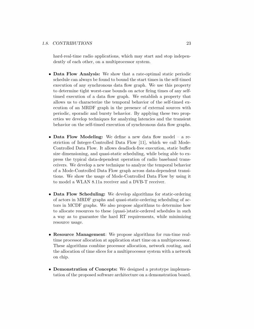
1.8. CONTRIBUTIONS 23
hard-real-time radio applications, which may start and stop indepen-dently of each other, on a multiprocessor system.
• Data Flow Analysis: We show that a rate-optimal static periodicschedule can always be found to bound the start times in the self-timedexecution of any synchronous data flow graph. We use this propertyto determine tight worst-case bounds on actor firing times of any self-timed execution of a data flow graph. We establish a property thatallows us to characterize the temporal behavior of the self-timed ex-ecution of an MRDF graph in the presence of external sources withperiodic, sporadic and bursty behavior. By applying these two prop-erties we develop techniques for analyzing latencies and the transientbehavior on the self-timed execution of synchronous data flow graphs.
• Data Flow Modeling: We define a new data flow model – a re-striction of Integer-Controlled Data Flow [11], which we call Mode-Controlled Data Flow. It allows deadlock-free execution, static buffersize dimensioning, and quasi-static scheduling, while being able to ex-press the typical data-dependent operation of radio baseband trans-ceivers. We develop a new technique to analyze the temporal behaviorof a Mode-Controlled Data Flow graph across data-dependent transi-tions. We show the usage of Mode-Controlled Data Flow by using itto model a WLAN 8.11a receiver and a DVB-T receiver.
• Data Flow Scheduling: We develop algorithms for static-orderingof actors in MRDF graphs and quasi-static-ordering scheduling of ac-tors in MCDF graphs. We also propose algorithms to determine howto allocate resources to these (quasi-)static-ordered schedules in sucha way as to guarantee the hard RT requirements, while minimizingresource usage.
• Resource Management: We propose algorithms for run-time real-time processor allocation at application start time on a multiprocessor.These algorithms combine processor allocation, network routing, andthe allocation of time slices for a multiprocessor system with a networkon chip.
• Demonstration of Concepts: We designed a prototype implemen-tation of the proposed software architecture on a demonstration board.

24 CHAPTER 1. SETTING THE STAGE
1.9 Thesis organization
The remainder of this thesis is organized as follows: in chapter 2, we makean evaluation of the problem as a whole, derive a set of design requirementsfrom product requirements, and propose an overall structure for the compi-lation flow and runtime software infrastructure of our solution. In chapter3, we review data flow models, and their analytical properties, and intro-duce mathematical notation for representing data flow graphs. In chapter 4,we present our methods for temporal analysis of the self-timed execution ofsynchronous data flow graphs, and how they can be used to give throughputand bounded latency guarantees for self-timed execution of a synchronousdata flow graph. Chapter 5 proposes a method to compute, at compile-time,resource budgets per radio, based on their Single-Rate Data Flow representa-tion. Chapter 6 proposes a new data flow analysis model, Mode-ControlledData Flow, that enables the expression of the data-dependent functionalbehavior of some radio transceivers, while still allowing for strict real-timeanalysis. This chapter also extends the scheduling techniques presented inChapter 5 to handle Mode-Controlled Data Flow. Chapter 7 discusses theproblem of allocating resources to a transceiver at run-time, based on pre-computed budgets. Chapter 8 describes a prototype implementation of thesoftware architecture, including the resource manager, run-time applicationsupport, and compile-time compiler/scheduler. Chapter 9 states our con-clusions and suggests future work.

Chapter 2
Software Framework
We present and analyze the requirements of our problem and design a Soft-ware Framework (SF) that addresses all of them. We start the chapter bydefining terminology and describing our hardware architecture model. Wethen inventorize the requirements that the SF must address. This is fol-lowed by a discussion of the chosen Model of Computation and the overallresource management strategy, including the choice of local schedulers andtask synchronization techniques. From this, we identify the main softwarecomponents of the solution and present an overview of the complete SF,including the compilation chain and the runtime support. We then give aquick overview of components such as the programming language and codegenerator, which will not be discussed in further detail in this thesis. Wecompare our proposal with related work and close the chapter by statingour conclusions.
2.1 Terminology
We will generically refer to a program that processes the baseband layer of awireless communication channel as a transceiver. A transceiver can be in-stantiated independently of other transceivers. We will refer to a transceiverinstance as a job. Each transceiver is programmed as a set of concurrentlyexecuting tasks. Since transceivers are streaming applications, the topol-ogy of the communication (i.e. the flow of data and control) between tasksis rather rigid. We refer to the set of tasks and the set of communicationchannels between them as the task graph of the transceiver. We say thata transceiver is installed in a device if the device is capable of instantiatingthe transceiver and executing that instance. We say that a transceiver is
25

26 CHAPTER 2. SOFTWARE FRAMEWORK
activated in a device when at least one instance of the transceiver is cur-rently prepared to execute – i.e. all its processes and data structures havebeen instantiated and the transceiver instance is only waiting for input data– or executing.
It is also useful to define more precisely what we mean by SoftwareFramework. We consider part of the software framework all the software-related concepts and components that are required in order to program,compile and run applications on the hardware platform. This includes:
1. A model of computation;
2. A programming language;
3. A scheduling and resource management strategy;
4. Application runtime support libraries (e.g., for inter-task communica-tion and synchronization, for job and task instantiation);
5. The runtime resource management and scheduling programs;
6. A temporal analysis model;
7. Temporal analysis algorithms and tools;
8. Compilation/mapping algorithms and tools;
9. Interfaces to the external world.
Our Software Framework must contain all of these components.
2.2 Hardware Architecture
In this thesis, we will assume as target template architecture a heterogeneousmultiprocessor system with many similarities to the architectures presentedin Section 1.5.
Our multiprocessor system template for baseband decoding, as depictedin Figure 2.1, includes one or more general-purpose ARM cores, to handlecontrol and generic functionality, one or more vector processors, each aninstance of the EVP [8] core, to handle detection, synchronization and de-modulation, and one or more Software Codec processors, that take care ofthe baseband coding and decoding functions. Besides these, the system hasan array of RF interfaces, and a memory-mapped interface to the external

2.2. HARDWARE ARCHITECTURE 27
world. Each processor has its own data and code memory, and caching isnot employed. The processors are interconnected by a multi-layer AHB bus,with every processor having both a master and a slave port connected tothis multi-layer bus. All masters are connected to all slaves, and thereforecommunication via posted writes to the consumer’s memory is always pos-sible between any two cores. This system template contains the essentialcharacteristics of a programmable platform for baseband. It does not usecaches because the improvement on average memory access performancethat they provide is not interesting for a hard RT system, that must bedesigned assuming worst-case timings. Our system employs dedicated localmemories per processor core and a simple, fully-connected multi-layer buswith slave-side arbitration to keep the communication flexible, predictable,and easy to handle.
A fully connected multi-layer bus architecture will not scale well with theincrease in the number of processors. In later sections of this thesis, we willextend our architecture with a Network-On-Chip, the Æthereal [31], that isdesigned to scale with the number of processors, since it does not requirefull connectivity. The Æthereal Network is particularly interesting for hardRT applications since it allows for the reservation of network resources perchannel to provide connections with guaranteed throughput and latency.
SOC Architectures and Infrastructures, Orlando Moreira, 31, January, 2008
CONFIDENTIAL 8
Abstract SDR Baseband HW architecture
On-chip interconnect
ARM
A Mem
NI
EVP
Mem
NI
CoDec
A Mem
NI
Source
NI
A
Sink
NI
Figure 2.1: Abstract target architecture template

28 CHAPTER 2. SOFTWARE FRAMEWORK
2.3 Requirements
In this section we will inventorize a number of important concerns that ourSF must address. These will be listed together, categorized only by domainof concern, to avoid over-categorization. It should be obvious from thelanguage employed whether a specific item relates to a strict requirement, adirective, or a nice-to-have property.
1. Application requirements
(a) The temporal behavior of jobs must be guaranteed. Aproof must be given that a transceiver meets the RT requirementsof the specific radio standard it implements.
(b) Jobs must be able to start and stop independently. Dur-ing device operation, a request to start executing a job may berandomly issued by an external source, at unknown times. Otherjobs may already be active at the time. For instances, a user istransferring information with a wireless LAN and tracking herposition with GPS, when a phone call arrives. A new transceiverinstance has to be activated, but the other radios should continueto operate without hiccups.
(c) The observable behavior of a running job cannot be af-fected by other jobs. This relates to our discussion on in-dependence of behavior in Section 1.6.3. The SF must assumethat a different set of jobs may be present in each device, andthat the composition of this set may change dynamically due topost-deployment upgrades. This implies that worst-case tempo-ral behavior has to be defined independently of the particularcombination of transceivers installed. Also, combining jobs inan execution environment should not result in changes to theirfunctional behavior (for instances, we should prevent that a jobcorrupts the memory space of another job).
(d) Transceivers must be independently deployable. This isbecause post-hardware deployment upgrades (such as new trans-ceivers being downloaded into the device by the end-user) anddifferentiated user settings (different set of transceivers per de-vice) must be possible. It implies that we either resort to sepa-rate compilation of transceivers, or transceivers are compiled inthe embedded platform itself.

2.3. REQUIREMENTS 29
2. Hardware requirements:
(a) The SF must cope with the limitations of the hardware.Some processing cores cannot support preemption. Because ofthis, and although preemptive scheduling is desirable in the sensethat it allows us to more effectively isolate the behavior of trans-ceivers, the SF must provide both preemptive and non-preemptivescheduling mechanisms. If available, memory virtualization canbe used to guarantee that a job cannot corrupt the memory of an-other job, protecting the system against violations of requirement1c. Many embedded processors, however, do not have support formemory virtualization or even memory protection. This meansthat requirement 1c cannot be fully met without rigorously in-specting the code that runs on these processors.
(b) Transceivers must be programmed in such a way as toallow efficient mappings of algorithms. Programming re-strictions and primitives provided to the programmer should al-low optimized usage of the hardware resources. This includes,for instances, the ability to exploit core intrinsics such as thespecial-purpose instructions of a vector processor.
3. Software Productivity requirements:
(a) Programming transceivers should be easy and intuitive.The goal of the system is to process baseband radio. The commonstructure of a baseband processing algorithm should be expressedin a natural and concise way.
(b) The SF should make it simple to re-use software com-ponents. Identical software functionality that is required bymany transceivers (such as inter-process communication libraries)should be provided as runtime support libraries, and not requirerepeated independent coding for each transceiver.
(c) Mapping should be as much as possible a “push button”process. Although it is easy for engineers to understand intu-itively the major concepts behind temporal analysis of concurrentapplications, many of its intricacies are difficult to understandand even more difficult to keep in mind at all times. Moreover,the more human intervention we have in the design flow, themore likely it is that errors are introduced. We want our SF toencapsulate as much as possible the RT analysis techniques, andrequire as little error-prone manual work as possible.

30 CHAPTER 2. SOFTWARE FRAMEWORK
(d) Porting transceivers to a different hardware platformshould be easy. Headset makers do not want to be tied to a spe-cific hardware platform, fearing to lose technological leadershipof the headset market to a single hardware supplier, as happenedto PC makers with respect to Intel in the 80s/90s [65]. Becauseof this, companies like Nokia and Samsung have relied on thestrategy of having more than one hardware supplier for modems.To make this strategy work, headset makers must have the abil-ity to quickly adapt software to a different hardware platform.However, in the last few years, the industry has moved more andmore to a model where the handset maker expects the provider ofthe modem hardware to also provide all the modem software, andportability may become less of an issue for the headset maker. Inthis case, portability becomes an internal issue for the hardwareprovider, who must internally handle several different hardwarearchitectures, both to the need for different architectures corre-sponding to different capability classes and price points, the on-going evolution of the hardware architectures, caused by changesand additions to the radio standards.
(e) Testing and debugging should be simple and manageable.The complexity of the verification process increases rapidly withthe amount of use-cases that must be supported. Our applica-tion requires support for a very large number of combinationsof transceivers installed in a device, and an even larger numberof combinations of active jobs. If a specific bug happens for aspecific combination of jobs, it may be very difficult to detect itand localize it. Debugging becomes easier when behavior inde-pendence, as per requirement 1c, is guaranteed.
4. Deployment requirements
(a) It should be possible (and reasonably easy) to port theSF to a different platform During the development process ofa hardware platform, many architectural decisions may change.The SF should be designed to adapt easily to hardware platformchanges. Moreover, it is frequent for subsequent releases of thesame embedded architecture to feature more cost-efficient hard-ware solutions. The SF should remain usable through these iter-ations. Another aspect of this is that a headset maker is likely toemploy different hardware architectures from different hardware

2.4. MODEL OF COMPUTATION 31
suppliers, as explained with respect to requirement 3d. An easilyportable SF also makes transceivers easier to port.
(b) All components of the SF should be useful in isolation,to allow for partial or phased adoption. One of the mainproblems in trying to popularize a new framework is that it is of-ten difficult for the potential adopters to accept at once a drasticchange to their way of working. If there is a specific advantagefor the potential adopter in a single component of the SF, adop-tion can be phased. The fact that the adopted component offerspalpable benefits individually, but larger (synergistic) benefits aspart of a whole integrated SF makes it a good introduction to (ora “Trojan horse” for) the complete framework.
2.3.1 Addressing the Requirements
Because timing predictability (item 1a) is the most important and strictestof our requirements we will take our major decisions in such a way as toaddress it, while taking the others into account whenever possible. Wehave identified in Chapter 1 that the choice of Model of Computation andResource Management framework are the essential ingredients in defininga predictable system. We will discuss these two choices in the followingsections.
2.4 Model of Computation
We opt to use SRDF as our base MoC, with extensions added to fit theapplication domain and fix the shortcomings of the model, without losingits valuable formal properties. Our extension to SRDF is called Mode-Controlled Data Flow and will be extensively discussed in Chapter 6. As aMoC, Single-Rate Data Flow has many advantages. We already hinted atthis in Chapter 1. For now, we will simply list its advantages and disadvan-tages without further discussion (a more in-depth look at the properties ofdata flow models will be postponed to Chapter 3). The main advantages ofSingle-Rate Data Flow are:
• The execution model is data-centric, which follows the natural struc-ture of streaming applications (therefore fitting requirement 3a);
• It separates the specification of the activation rules and data produc-tion/consumption patterns of a task (an actor) from its functional

32 CHAPTER 2. SOFTWARE FRAMEWORK
specification; this separation of concerns eases the programming effort(requirement 3a) and improves transceiver portability (requirement3d);
• Strong formal properties: SRDF is functionally deterministic, tempo-rally monotonic and amenable to temporal analysis techniques, whichaddresses our main requirement, predictability (requirement 1a); more-over, schedules can be statically ordered, reducing runtime schedulingoverhead, in accordance to our need for efficient mappings (require-ment 2b);
• SRDF can be both employed as a timing analysis model and a pro-gramming model; the same abstraction can be used for all stages ofthe mapping process; a correct-by-construction analysis model can beeasily and automatically derived from the specification, and resourceallocation decisions can be modeled as SRDF components; this allowsfor resource budgeting – enabling our strategy to accomplish indepen-dent job behavior (requirement 1c) – and automation of the mappingprocess (requirement 3c)
The main limitations of Single-Rate Data Flow are:
• Shortcomings of the analysis techniques. At the moment westarted our work, the temporal analysis of SRDF graphs which werenot fully-statically scheduled was limited to the analytical determina-tion of a minimum guaranteed throughput on long execution runs. La-tency analysis techniques were not available, nor were there any waysto guarantee strictly periodic behavior of output production withoutapplying a fully static schedule. In Chapter 4, we propose extensionsto existing analysis techniques to deal with these shortcomings.
• Limited expressive power. SRDF actors must have fixed rates ofdata production/consumption. Many extensions to SRDF have beenproposed that improve on this limitation. These, however, tend tolose all the interesting temporal properties. We will give an overviewof these data flow models in Chapter 3. In Chapter 6, we will pro-pose Mode-Controlled Data Flow (MCDF), a extension designed toconveniently express SDR applications, without losing the ability toperform temporal analysis.
To use our extension of SRDF as a programming model, we must enforcethe usage of SRDF constructs. This calls for a programming language that

2.5. RESOURCE MANAGEMENT OPTIONS AND CHOICES 33
restricts the user to specify valid data-flow programs. For this effect, we willemploy the LIME [55] language. We will give a quick overview of the basicsyntax of LIME in section 2.7 of this chapter and extend it to MCDF inChapter 6.
2.5 Resource Management Options and Choices
The decisions involved in scheduling the resources of a multi-processor sys-tem include deciding where to execute tasks (processor assignment) andwhen to execute tasks (task ordering and task start times). It is common toclassify resource management frameworks with respect to when each decisionis taken, that is, whether it is done when the application code is generated(compile time) or while the system is in operation (runtime). When a deci-sion is made at compile time, it is referred to as a static decision. When adecision is made at runtime, it is referred to as a dynamic decision. We willdiscuss options and motivate the choice taken for our SF design in Section2.5.1.
Another decision to be taken is with respect to the way in which tasksynchronization is achieved across the multi-processor system. This is re-lated with the decision on whether scheduling is handled in a centralized,global fashion, or in a distributed, local way. We wiil discuss our choices inSection 2.5.2.
2.5.1 Deciding when to decide
A survey of the traditional techniques to handle resource management andscheduling of data-flow graphs in a hard-real-time multi-processor systemcan be found in [82]. These techniques range from fully static to fully dy-namic scheduling. Our particular scenario, where jobs are expected to enterand leave the system at any time during operation (stated in requirement1b), is not considered.
At one end of the range, we have fully static scheduling. In fully staticscheduling, the time at which all activities concerning the execution of a pro-gram happen is decided at compile time. Combined fully static scheduling ofall jobs does not work here because it requires that an exact, unchangeablecombination of jobs is known at compile time, fixed execution times for alltasks, fixed communication times for all channels, and a global concept oftime across the system.
At the other end of the range, we have fully dynamic scheduling, wereall activities are scheduled at runtime. Fully dynamic scheduling is in gen-
34 CHAPTER 2. SOFTWARE FRAMEWORK
eral possible but impractical. One reason is that it causes high runtimeoverheads and makes it particularly difficult to give guarantees of temporalbehavior. Another reason is that it requires the system to efficiently handletask migration, without affecting the worst-case temporal behavior of jobs.
A traditional way of scheduling a single job is by employing static as-signment. In static assignment, processor assignment is done at compiletime, but local scheduling is handled at runtime. This does not work in ourcase, as this strategy cannot take into account that, at the time that a job isactivated, an unknown mix of jobs is already running, and using resources.For static assignment to work, the state of the system at the time that thejob is started must be known.
An extension of the previous solution that is used in cases where severaldifferent combinations of jobs need to be supported is the configuration-based approach (used, for instances, in CPA [85]). For each job combination,a separate optimal static schedule is derived at compile time and stored ina look-up table. During operation, when there is a request to start a job,the runtime system checks which jobs are active and selects the appropriateconfiguration. This approach has insurmountable problems with respect toour requirements. First, a different configuration has to be stored for eachcombination of jobs, and therefore the number of configurations may growexponentially with the number of jobs that must be supported (althoughin practice there are many job combinations that do not need to be sup-ported). Second, according to our requirements, not all jobs are known atdesign-time, which means that every time a new job is added to a system,it will force a whole new set of configurations for all jobs to be compiled.Third, as different configurations must assign different resources to eachjob, it becomes difficult to assure continuity of execution of already runningjobs during reconfiguration. If continuity is required, as stated on our re-quirement 1c, then either there are means for task migration with real-timeguarantees,or a configuration must be generated for each transition of a job-mix to another, instead of for each job-mix, which becomes unpractical foreven very small sets of jobs.
Our approach is derived from static assignment. However, whereas intraditional static assignment the mapping of tasks to processors is done atcompile time, in our case this is done at a specific phase during runtime. Atcompile time, we calculate independent resource budgets per job. Duringruntime, two distinct types of temporal phases alternate: reconfigurationphase and steady-state execution phase. During reconfiguration phases,resources are allocated to jobs, while during steady-state phases resourceallocation is fixed. Our strategy can also be compared with semi-static tech-

2.5. RESOURCE MANAGEMENT OPTIONS AND CHOICES 35
niques [16], where system execution is divided in phases and the resourceallocation is redone at the beginning of each phase. But while in semi-staticsystems phases are typically periodical, in our case reconfiguration phasesare triggered when there is a request to start a job.
Our strategy has some similarities with time-multiplexing schedulingstrategies such as gang scheduling [19]. Our jobs correspond roughly toa gang in gang scheduling, i.e. a group of tasks with data-dependencies.There is, however, an important difference in granularity: in gang schedul-ing, time-multiplexing is global, i.e., the temporal slots are uniform acrossall processors, and synchronized context-switching is required. In our case,time-multiplexing is local to each individual processing element and may beobtained by using any single-processor scheduling mechanism such as TimeDivision Multiplex (TDM), Round-Robin or even Rate-Monotonic. Ourscheduling strategy has several advantages over gang scheduling: it does notrequire the global synchronization of context switching that gang schedulingneeds and which hinders design scalability; it leaves less unused resourcesbecause its time-sharing is very fine-grained; and it allows for different localscheduling mechanisms to be used in different processors.
In Table 2.1 we summarize the scheduling strategies we inventorized.From left to right, decisions become more dynamic. The more dynamic thescheduling decisions become, the more difficult it is to give guarantees oftiming behavior. With our approach, it is impossible to guarantee that ajob can always be started, as it may be the case that there are no resourcesavailable at the time the start request arrives or, even in the case that the re-sources are available, it may be that it is impossible to find the solution: theresource allocation problem, as we shall show in Chapter 7 is NP-complete,even when we disregard memory fragmentation, and, therefore, it is not pos-sible to exhaustively search for all possible resource allocations in efficienttime.
This level of dynamicity, however, is necessary because of requirements1b and 1d. However, it must be noted that these requirements are only withrespect to the scheduling between different jobs. Since we know at compiletime each job in its entirety, we can alleviate the amount of work that mustbe done at runtime by statically clustering and ordering tasks within a job.This will be discussed at length in Chapters 5 and 6. For the moment, wejust would like the reader to retain the idea that task ordering is handleddynamically between jobs, but as statically as possible within a job.

36 CHAPTER 2. SOFTWARE FRAMEWORK
Fully Static Static Configuration Our FullyStatic Order Assignm. Based Approach Dynamic
Processor Static per Semi-Assignment Static Static Static Configuration Dynamic DynamicTask Static per Semi-Ordering Static Static Static Configuration Dynamic DynamicTaskScheduling Static Dynamic Dynamic Dynamic Dynamic Dynamic
Table 2.1: Scheduling strategies with respect to the time of decision.
2.5.2 Task Synchronization
On a typical embedded heterogeneous multiprocessor platform, a general-purpose processor is used to start task executions on all processing ele-ments (accelerators and digital-signal processors), employing the assistanceof DMAs to transfer data from one local memory to another. The basicmodel of execution is essentially single-threaded, with the application con-trol residing singly on the general-purpose processor, acting as a master. Allother processing elements are slaves, their tasks being activated by remoteprocedure calls. Some concurrency can be exploited since the control threaddoes not need to wait for a remote procedure call to terminate before invok-ing another procedure call on a different processing element. This strategymay work well when a single, static job is being executed, since not many ac-tivities are executed in parallel, and they are all part of the same application.The main limitation of such an approach is that the master is a centralizedresource that stands in the critical path of all data transactions and controlflow going on in the system. Every time a slave finishes an activity, either itmust report it to the master (normally through an interrupt), or the mastercontinuously polls the slaves for events. This does not scale well with anincrease in the number of parallel tasks. We opt for distributed data-drivensynchronization, where producing tasks inform their consuming tasks aboutavailability of data through a FIFO abstraction, and consuming tasks areactivated once data is available. If more than a single task is available at atime, a scheduler local to the processing element decides according to somepre-defined policy what task should execute. Not only does this solve theproblem of scalability well, it also fits much better our chosen programmingmodel.
However, not all accelerators are “smart” enough to be used in thisway, as their only mode of operation is based on the remote procedure callmodel, that is, a master indicates to them where input data in memory, wereoutput data must be placed, and starts execution. Such hardware does notsupport a distributed synchronization model. In such cases, the master/slaveinterface must be applied. We will say that in such a case the schedule of
2.5. RESOURCE MANAGEMENT OPTIONS AND CHOICES 37
the slave is hosted by a master, meaning that the master activates a task inthe slave and then waits for the task to complete. It is assumed that eachslave has a single master, and, since the master waits for task completion,reservation of the host’s resources corresponds to reservation of the slave’sresources.
2.5.3 Choice of Local Schedulers
It is important to choose well the scheduling policies of the local task sched-ulers. In a budget-based approach, the local schedulers must enable thereservation of resources and give subsequent guarantees of worst-case com-pletion times. In other words, there must be a direct computable relationbetween a resource allocation and the worst-case completion time of thetask. Also, it is necessary that a schedulability check can be performed suchthat, knowing all the tasks allocated to a processor, their timing require-ments and their resource allocation, one can infer whether all tasks will beable to meet their real-time constraints. This requirement rules out popularschedulers, such as preemptive fixed-priority. In a preemptive fixed-priorityscheme, each task is assigned a priority and, whenever a task is ready, it willrun once no tasks of higher priority are ready. In this scheme, a very highpriority task can effectively delay indefinitely the execution of other tasks,depending on the time it becomes active and on how often it is activated. Itis therefore impossible to give any guarantees of timely completion to anyother tasks in the system without fully characterizing the best and worstcase of the activation pattern of the high priority task. Consider for in-stances that the highest priority task on a given processor, task A, is readywhenever a task B running on a different processor generates data. If B gen-erates data faster, then task A becomes ready more often, and less resourceswill be available to any other ready task running on the same processor asA, potentially resulting in these other tasks missing their deadlines. This iswhat is called a timing (or scheduling) anomaly [64], i.e., situations wherelocal worst-cases do not entail a global worst-case.
Although there are many schedulers that fit our requirements, in thisthesis we will consider just two, not so much because of their efficiency, butfor their simplicity. In processors that support preemption, we will employ aTime-Division Multiplex (TDM) scheduler, also known as a slicing scheduler.A TDM scheduler has a period P and a list of assigned tasks. Any task Aassigned to the scheduler is assigned a time slice SA. For every period, thescheduler will allow the task to run for a time interval equal to SA, beforepreempting it to execute the next task in the list. Knowing the period
38 CHAPTER 2. SOFTWARE FRAMEWORK
of the TDM scheduler, the worst-case execution time of a task – the timeinterval between the moment when the task becomes ready and terminationwhen the task runs alone in the processor without resource sharing – andits allocated slice, one can compute the task’s worst-case response time –the time interval between the moment when the task becomes ready andtermination when running under supervision of the local scheduler – see [7].Also, checking if a slice SA can be mapped to a TDM scheduler with periodP amounts to checking if the sum of SA with all other slices already allocatedto the processor is lesser or equal to P.
TDM requires a preemptive scheduler. For processors not capable ofimplementing a preemptive scheduler, we will use a Non-Preemptive RoundRobin (NPRR) scheduler. An NPRR scheduler keeps a list of the tasksallocated to it. It constantly goes through that list, checking at each time ifa task is ready. If it is, it allows it to execute until it terminates. If the taskis not ready, it checks the next task for readiness, and so on. If we know theworst-case execution time of a task we know that the worst-case responsetime of the task is equal to the sum of the worst-case execution times of alltasks allocated to the processor.
We will discuss how to compute response times and assign resource bud-gets to tasks on TDM and NPRR schedulers in Chapter 5.
2.6 Proposed Solution Overview
Our approach addresses the two main sources of unpredictable behavior. Weaddress algorithmic (application intrinsic) unpredictability by employing astrict concurrent Model of Computation (MoC). The restrictions of the MoCare enforced by a programming language, LIME [55].
We address resource sharing (inter-application) unpredictability by de-signing the runtime resource management strategy to preserve the worst-casetemporal behavior of each application. A centralized resource manager en-forces admission control and budget-based resource allocation. Jobs (trans-ceiver instances) explicitly request at start time for the resources they needto meet their HRT requirements. Our MoC supports this, by doubling as atemporal analysis model where budgeting decisions can be represented, asalready explained in Chapter 1.
We will now give an overview of the proposed Operating System andProgramming Flow.

2.6. PROPOSED SOLUTION OVERVIEW 39
2.6.1 Operating system
Figure 2.2 depicts the software stack running on our system. Acceleratorsare not depicted as their schedule is hosted by the programmable cores.The interface to start/stop baseband jobs is done via the Resource Manager(RM). The RM receives requests from a Central Resource Manager (CRM),as specified in the multi-radio functional architecture proposed in [1]. Uponan admission control request, the RM demands the Configuration Manager(also specified in [1]) for a transceiver budget, precomputed by our program-ming flow (described below). The RM tries to find a mapping that fits theavailable platform resources. If it finds one, it informs the CRM that thejob may be started. The CRM can now instruct the RM to start the job.The RM invokes the Network Manager API to resume all tasks of the job.All cores support a FIFO API, and a local scheduler. In our demonstrator,the Network Manager, local Schedulers and the FIFO API are part of NXPSemiconductors’ Sea-of-DPSs (SoD), a lightweight streaming framework formulti-DSP systems. It provides three OS modules: Streaming Kernelsare single-core task schedulers; the Streaming API provides FIFO read-/write primitives; the Network Manager API creates and destroys tasksand FIFOs on the streaming kernels.
ARM
StreamingKernel
Radio Functions
ARM
StreamingKernel
Radio Functions
CentralResourceManager(external)
RTOS (μCOS)
Network Manager
ARM
ConfigurationManager(external)
ARM
StreamingKernel
Transceiver Tasks
EVP
StreamingKernel
TransceiverTasks
Communication Infrastructure
BBResource Manager
Streaming APIstart/stop/connect
tasks
Figure 2.2: Multi-radio runtime.

40 CHAPTER 2. SOFTWARE FRAMEWORK
2.6.2 Programming and Mapping Flow
The resource budget of a transceiver is computed at compile time as depictedin Figure 2.3. The input consists of LIME-compliant C components, imple-menting DF actors, and the Transceiver Graph, a LIME file that describeshow components communicate and synchronize with each other. From these,the front-end extracts a DF model, which is fed to the scheduler. The sched-uler also requires a machine description file, describing types and numberof cores in the multiprocessor, their local scheduling mechanism, memorysegments available, and their sizes. Another input of the scheduler is apartial mapping that provides the scheduler with bindings of LIME compo-nents to processor types, and worst-case execution times for all (compiled)components. This file can also be used by the designer to constrain theDF scheduler, by providing maximum values for any budgeted resource.The scheduler also requires the programmer to specify timing requirements.These are minimum throughput and/or maximum latencies.
The scheduler searches for a resource budget for each task and channelthat meets the HRT requirements and fits in the multiprocessor resources.It clusters tasks, and computes, per cluster, a quasi-static execution order(explained in Chapter 6), on-line scheduler settings, and, per inter-clusterFIFO, a buffer size requirement. It outputs these as a Transceiver Budget.It also generates a description of how the original software components areordered within the clusters. The Code Generator uses this to generate atask wrapper per cluster, with calls to the Streaming API for inter-clustercommunication and synchronization. Each task wrapper is fed to a core-specific C compiler to generate dynamically loadable object code.
In summary, the DF scheduler solves resource conflicts within a trans-ceiver through clustering and ordering, while the Resource Manager and theStreaming Kernels resolve resource conflicts among transceivers, based onbudgets computed at compile time. This division of tasks is done consider-ing that extensive analysis of dependencies cannot be performed efficientlyat runtime, and that the set of transceivers is not known at compile time.
2.7 Programming Language
LIME [55] is designed to express applications in multiple data flow MoCs.LIME uses two distinct formats. The graph is specified by an XML schemacalled GXF. Communication and synchronization are modeled through portsattached to LIME components.
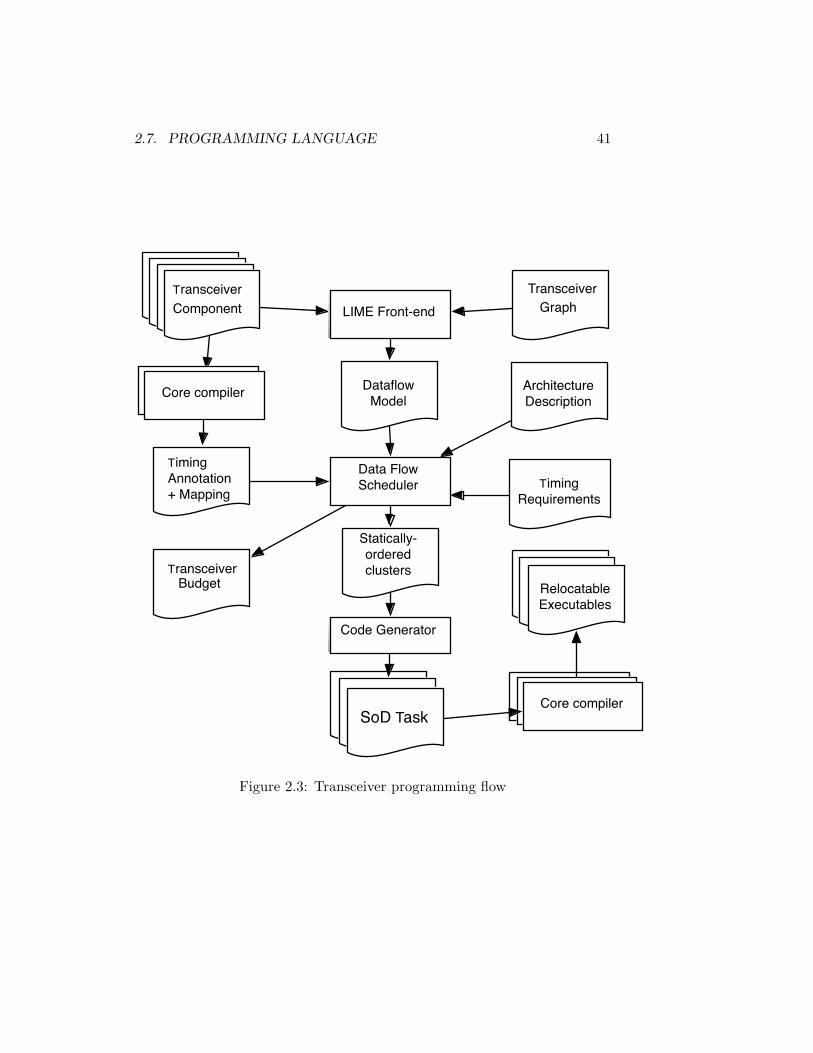
2.7. PROGRAMMING LANGUAGE 41
LIME Front-endTransceiver
Graph
Radio SWComponentsRadio SWComponents
Radio SWTransceiverComponent
Analysis Dataflow
Model
Data FlowScheduler
Architecture Description
TimingAnnotation+ Mapping
Timing Requirements
Statically-ordered clustersTransceiver
Budget
Code Generator
Core compilerCore compiler
T iming AnnotationTiming AnnotationTiming
AnnotationSoD TaskCore compilerCore compilerCore compiler
RelocatableExecutables
Figure 2.3: Transceiver programming flow

42 CHAPTER 2. SOFTWARE FRAMEWORK
A component is a C module, corresponding to a DF actor. The signal-processing algorithms are specified in C99. Processor-specific intrinsicsand platform-specific accelerators can be used. This organization isolatesplatform-specific functionality in some components and supports portabil-ity of others.
The signature of the top-level C function in a module declares the portsand firing conditions of the actor. Each argument corresponds to a portand it is declared as an array of the type of data received. The variablename provides the name of the port; the array size specifier represents aproduction/consumption rate, while the presence/absence of the const typemodifier indicates whether the port is input or output. For example, a Gainactor that outputs the value of the input sample multiplied by 5 can bewritten like this:
void Gain ( const i n t in [ 1 ] , i n t out [ 1 ] )out [0 ]= in [ 0 ] ∗ 5 ;
Since arguments are arrays and C arrays are pointers, the Code Gener-ator is free to decide how to implement data acquisition and pass pointersto the C function. It can use any FIFO implementation (blocking/non-blocking, in-place/double buffered, with/without synchronization), or evenreplace FIFOs for local buffers when combined with clustering. This enablesautomatic code generation of all the communication primitives, allowing re-use and improving efficiency of the implementation. It also makes the codeeasier to port, as different, hardware-specific implementations of FIFO com-munication can be generated by simply re-writing the Code Generator.
Consider the SRDF graph in Figure 1.7(a). Assume the prototypes of Aand B are
void A ( i n t out [ 1 ] ) ;void B( const i n t in [ 1 ] ) ;
If the DF scheduler creates separate tasks for A and B, the generatedtask wrappers, using the Streaming API, are:
void taskA ( channel f i f o )i n t ∗p ;i f ! ( p = checkWrite ( f i f o ) ) re turn ;A(p ) ;Write ( f i f o , p ) ;updateWrite ( f i f o ) ;
void taskB ( channel f i f o )i n t i ;i f ! ( checkRead ( f i f o ) ) re turn ;i=Read( f i f o ) ;

2.8. RELATED WORK 43
B(& i ) ;updateRead ( f i f o ) ;
Instead, A and B can be clustered and statically ordered and the CodeGenerator instructed to produce a single task wrapper:
void taskAB () i n t i ; A(& i ) ; B(& i ) ;
In this example, clustering saves 1 task wrapper, 6 API calls per firing,and 1 FIFO, and reduces the number of task to be scheduled (and thereforethe scheduling overhead) by 1 task.
The output port of actor A can be connected to the input port of B by aGXF statement equivalent to “FIFO f1 connects port A.out to port B.in”.
Besides FIFOs, LIME allows actors to connect to initialization edges,for delay initialization; and to state edges, to carry actor state across firings(actors are otherwise stateless).
LIME can express several DF flavors. Strict compliance to MCDF isverified by checking the construction rules described in Chapter 6. Sinceactors are written in C, processor intrinsics and core-specific C compileroptimizations can be exploited. This cannot be done for dedicated languageslike StreamIt [90]. As it does not explicitly code communication with APIcalls, nor allows interleaving of communication with computation, LIMEenables automatic extraction of MCDF analysis models, and generation oftasks per cluster with platform-specific communication. This is not possiblefor API-based extensions of C such as MPI [37] (although MPI could beused as target for code generation instead of SoD).
2.8 Related Work
There have been a few programming models and software architectures pro-posed for SDR.
One software architecture that is widely used for SDR for military ap-plications is the Software Components Architecture (SCA) [47], proposedby the the United States Army. Its uses an object-oriented programmingmodel. It allows allocation of resources to a transceiver at start time. Itdoes not require a disciplined use of concurrency, relying on general-purposemulti-threading. Consequently, temporal analysis is not possible, and timingmust be verified through exhaustive simulation of use-cases.
Another software architecture for SDR is proposed in [36]. It uses adependency graph for compile time scheduling. The graph is drawn man-ually by the designer, and may not conform to the actual implementation,which is programmed using multi-threading primitives. Real-time analysis
44 CHAPTER 2. SOFTWARE FRAMEWORK
is not performed, and validation is done by extensive simulation. For run-time support, it employs a multi-threaded operating system, and time-slicedschedulers. This work does not address multi-radio. The authors stress thatverification of the multi-threaded program is the most complex, time con-suming part of the design.
In [61], a programming language and flow that handle single-radio arepresented. HRT behavior is specified by a synchronous language. Syn-chronous languages have difficulties in dealing with multiple independentapplications: separate compilation, if not impossible, is difficult; pipelinedbehavior and the effect on timing of runtime schedulers is not handled. Theargument against using synchronous languages in this context is rather long,mostly because many attempts have been made recently to partially fix theshortcomings of the approach; in [92] the subject is discussed in more detail.
2.9 Conclusions
HRT multi-radio requires a budgeted, admission-controlled approach to re-source management, that isolates the worst-case behavior of transceivers.Furthermore, a choice must be made about what part of resource allocationis done at compile time, and which part of resource allocation must be doneat run time.
HRT guarantees require a Model of Computation amenable to tempo-ral analysis. We depart from Single-Rate Data flow which we will extendto Mode-Controlled Data Flow, which is customized to express the limiteddata dependent behavior of transceivers. The MoC must provide a tempo-ral analysis model that can double as a programming model to express thelimited concurrent behavior of transceivers and hardware budgeting deci-sions. DF also acts as a component model that isolates computation fromcommunication, making task interfaces explicit, and improving code porta-bility. With LIME, the programmer can write highly optimized sequentialcode for each task, and specify communication at an abstract level. Thisreduces concurrency coding errors, and saves programming effort, as callsto communication APIs are automatically generated at compile time.
The importance of combining a strict MoC with a programming languagethat enforces it to provide correct-by-construction models for temporal anal-ysis and scheduling cannot be overemphasized. We previously tried directusage of concurrent libraries such as SoD’s by the programmer, with manualextraction of a DF model by an expert. This was a long and hard process,riddled with errors and wrong assumptions. Furthermore, as mapping deci-

2.9. CONCLUSIONS 45
sions were manually implemented, guarantees of a correct final implementa-tion could not be given, and extensive testing was required. Our approachgreatly reduces the verification effort and enables HRT guarantees.

46 CHAPTER 2. SOFTWARE FRAMEWORK

Chapter 3
Data Flow ComputationModels
In the previous chapters, we justified our choice for data flow as the basisfor our model of computation. There are many flavors of data flow. Theones that are interesting to our work are mostly the variants that exhibitbehavior which is independent of data values, because of their analyticalproperties and the variants with deterministic, data value dependent behav-ior, because of their expressivity. In this chapter, we present the notationfor data flow models that we will use throughout the thesis, and the proper-ties of several data flow computation models that are relevant to our work.This is reference material and can, for the most, be found elsewhere in theliterature [81],[58],[82], [10].
3.1 Graphs
A directed graph G is an ordered pair G = (V,E), where V is the setof vertexes or nodes and E is the set of edges or arcs. Each edge isan ordered pair (i, j) where i, j ∈ V . If e = (i, j) ∈ E, we say that e isdirected from i to j. i is said to be the source node of e and j the sinknode of e. We also denote the source and sink nodes of e as src(e) andsnk(e), respectively.
3.1.1 Paths and Cycles in a Graph
A path in a directed graph is a finite, nonempty sequence (e1, e2, ..., en) ofedges such that snk(ei) = src(ei+1), for i = 1, 2, ..., n− 1. We say that path
47
48 CHAPTER 3. DATA FLOW COMPUTATION MODELS
(e1, e2, ..., en) is directed from src(e1) to snk(en); we also say that this pathtraverses src(e1), src(e2), ...src(en) and snk(en); the path is simple if eachnode is only traversed once, that is src(e1), src(e2), ...src(en), snk(en) are alldistinct; the path is a circuit if it contains edges ek and ek+m such thatsrc(ek) = snk(ek+m),m ≥ 0; a cycle is a path such that the subsequence(e1, e2, ..., en−1) is a simple path and src(e1) = snk(en).
3.2 Multi-Rate Data Flow Graphs
A Multi-Rate Data Flow (MRDF) graph —also known as Synchronous DataFlow [58], [82] — is a directed graph, where nodes are referred to as actors,and represent time consuming entities, and edges are referred to as arcs andrepresent FIFO queues that direct values from the output of an actor tothe input of another. Data is transported in discrete chunks, referred toas tokens. When an actor is activated by data availability it is said to befired. The condition that must be satisfied for an actor to fire is calledthe firing rule. MRDF prescribes strict firing rules: the number of tokensproduced (consumed) by the actor on each output (input) edge per firing isfixed and known at compile time. During an execution of a data flow graph,all the actors may fire a potentially infinite number of times.
In a timed MRDF graph, actors have a valuation t : V → N0; t(i) is theexecution time of i. Arcs have a valuation d : E → N0; d(i, j) is called thedelay of arc (i, j) and represents the number of initial tokens in arc (i, j).
Arcs have two valuations associated with them: prod : E → N andcons : E → N. prod(e) gives the constant number of tokens produced bysrc(e) on e in each firing and cons(e) gives the constant number of tokensconsumed by snk(e) in each firing.
A timed MRDF is defined by a tuple (V,E, t, d, prod, cons).Figure 3.1, we depict a MRDF graph with three actors A, B and C.
Arrows represent arcs, with the arrowhead indicating the direction fromproduction to consumption. Both arrow endpoints are annotated with theproduction/consumption rate of the producing/consuming actor in that arc.The black dots in an arc represent the delay (the number of initial tokens)on the arc.
Radio transceivers are applications that process data streams. This ofteninvolves computations on indefinitely long data sequences. Because of this,we are mainly interested in MRDF graphs that can be executed in a non-terminating fashion. Consequently, we must be able to obtain schedules thatcan run infinitely using a finite amount of physical memory. We say that

3.2. MULTI-RATE DATA FLOW GRAPHS 49
A B C2 3 1 2
31
Figure 3.1: Multi-rate data flow example.
a MRDF is correctly constructed if it can be scheduled periodically using afinite amount of memory.
If there exists a fixed number of firings of each actor in a given MRDFgraph that brings the graph to its initial token distribution and the graphis deadlock-free (how to check this will be explained in Section 3.3, then itcan be scheduled periodically, and thus it can run within a finite amount ofmemory. If r is a vector of integer values such that each r(i) represents thenumber of times that an actor i must be executed to bring the graph to itsinitial token distribution, then, for each edge (i, j) ∈ E it must hold thatthe number of tokens produced over r(i) firings of the producing actor i,and the number of tokens produced over r(j) firings of the consuming actorj is the same, that is:
r(i).prod(i, j) = r(j) · cons(i, j). (3.1)
The set of equations thus obtained is normally referred to as the balanceequations of a graph.
It is convenient to represent the balance equations in matrix form.The MRDF graph G(V,E, t, d, prod, cons) can be represented by its
topology matrix, T . The topology matrix contains one column per eachnode b in N and one row per each edge a in E. The value of element (a, b)is given by:
T (a, b) =
prod(ea) if src(ea) = vb ∧ snk(ea) 6= vb
−cons(ea) if snk(ea) = vb ∧ src(ea) 6= vb
prod(ea)− cons(ea) if snk(ea) = src(ea) = vb
0 otherwise
(3.2)
where ea ∈ E and vb ∈ V , a ∈ 1, 2...|E| and b ∈ 1, ...|V |.The system of balance equations of Equation 3.1 can then be expressed
in matrix form as:
T .~r = ~0 (3.3)

50 CHAPTER 3. DATA FLOW COMPUTATION MODELS
where ~0 is a column vector full of zeros, and ~r is a column vector.The repetition vector for a correctly constructed MRDF graph with
|V | actors numbered 1 to |V | is a column vector of length |V |, and cor-responds to the smallest positive integer vector ~r which is a solution ofEquation 3.3. If each actor va is fired a number of times equal to the ath
entry of ~r, then the number of tokens per edge of the MRDF graph is equalto what it was in the initial state. The repetition vector r is useful for gen-erating cyclic schedules for MRDF graphs. In addition, it will only exist ifthe MRDF graph is correctly constructed (see [57]). The repetition vectorcan be computed in polynomial time [57].
For the graph in Figure 3.1 the repetition vector is [3 2 1]. If theproduction rate of actor C were 4 instead of 3, the balance equations wouldnot have a solution other then a null vector.
An iteration of an MRDF graph is a set of actor firings such that eachactor in the graph executes a number of times equal to its repetition vectorentry. Therefore, in an iteration, each actor fires as many times as indicatedby the repetition vector.
In this thesis, we will consider only correctly constructed MRDF graphs.An MRDF is said to be First-In-First-Out (FIFO) if tokens cannot over-take each other in an actor. This means that between any two firings of thesame actor, the first one to start is always the first one to produce outputs.If s(i, k) is the start time on a given execution of an MRDF graph of iter-ation k of actor i and t(i, k) is the execution time of iteration k of actor i,then the MRDF is FIFO if for any execution of the MRDF graph it holdsthat
s(i, k) + t(i, k) < s(i, k + 1) + t(i, k + 1). (3.4)
If an actor either has a constant execution time or belongs to a cyclewith a single delay for the MRDF, it conserves the FIFO property (see [79],[3]). We will only consider MRDF graphs that have the FIFO property.FIFO MRDF graphs are deterministic, since for each actor, independentlyof the time of arrival of tokens to the input queues, for the same values inthe input queues, the same values are produced in the output queues.
An MRDF graph is monotonic in time execution. Consider a FIFOMRDF graph G = (V,E), with time valuation t(i). Say that schedulefunction s(i, k) represents the time at which the instance k of actor i ∈ Vis fired on a valid schedule of G. Consider now that t(i) is replaced by anew valuation t′(i), such that t′(i) ≤ t(i),∀i ∈ V . Monotonicity in timeexecution of G means that any valid schedule s(i, k) for time valuation t(i)is also admissible for time valuation t′(i). Intuitively, earlier termination of

3.3. SINGLE RATE DATA FLOW 51
an actor firing cannot cause other firings to occur later. This is because thefiring rule of an MRDF actor is determined by the latest required input tokento arrive and firing rules are fixed. If an input arrives earlier, it cannot causethe actor to fire later, and therefore it cannot cause the actor to produceoutputs later.
3.3 Single Rate Data Flow
An MRDF graph in which, for every edge e ∈ E, it holds that prod(e) =cons(e), is a Single Rate Data Flow (SRDF) graph. Any MRDF graphcan be converted into an equivalent SRDF graph. Each actor i is replacedby r(i) copies of itself, each representing a particular firing of the actorwithin each iteration of the graph. That is, for any given actor i in theMRDF graph with an r(i) entry in the repetition vector, if its copies in theequivalent SRDF graph are represented as ip, p = 0, 1...r(i)− 1, the firing kof ip corresponds to the firing k.r(i) + p of the original MRDF actor i. Theinput and output ports of these nodes are connected in such a way that thetokens produced and consumed by every firing of each actor in the SRDFgraph remains identical to that in the MRDF graph (see [82]).
Figure 3.2(a) depicts an MRDF graph. The SRDF-equivalent of thisgraph is depicted in Figure 3.2(b). The repetition vector of the MRDFgraph is [3 2]. The SRDF-equivalent graph has as many copies of eachactor as the number of repetitions of that actor in the repetitions vector.Each arc in the MRDF graph is represented by arcs between the copies. The4 initial tokens on the (A,B) edge are consumed by the first 4 consumptionsof tokens by copies of B. This essentially determines which copies of Aprovide tokens for which copies of B.
SRDF graphs have very useful analytical properties. A SRDF graph isdeadlock-free if and only if there is at least one delay in every cycle [82].A graph is deadlocked when there is a cyclic dependency where two actorscannot fire because each requires the other one to fire in order to obtainthe data required for it to fire itself. The cycle mean of a cycle c in aSRDF graph is defined as µc =
Pi∈N(c) tiPe∈E(c) de
, where N(c) is the set of all nodes
traversed by cycle c and E(c) is the set of all edges traversed by cycle c.The Maximum Cycle Mean (MCM) µ(G) of a SRDF graph G is
defined as:
µ(G) = maxc∈C(G)
∑i∈N(c) ti∑
(e∈E(c) de(3.5)

52 CHAPTER 3. DATA FLOW COMPUTATION MODELS
BA2 3
(a)
B2A1
A2
A3B1
(b)
Figure 3.2: An MRDF graph and its SRDF-equivalent graph.

3.4. INTEGER DATA FLOW 53
where C(G) is the set of simple cycles in graph G.As we shall discuss in Chapter 4, the MCM of a SRDF graph is equivalent
to the inverse of its maximum attainable throughput. Many algorithms ofpolynomial complexity have been proposed to find the MCM (see [17] foran overview).
3.4 Integer Data Flow
In his PhD thesis, Buck introduces Boolean Data Flow and Integer DataFlow. In Integer Data Flow (IDF), the ports of actors are labeled as be-ing either data ports or control ports. If an actor has no control ports, itbehaves just like a MRDF actor. If an actor has a control port, however,the consumption rates are no longer fixed. We shall refer to these actors asvariable-rate actors.
Buck defines two types of control tokens:
• Type 1 - case control : the number of tokens transferred by thevariable-rate actor receiving this type of control token from/to eachof its data in/out ports is either constant or zero, depending on thevalue of the control token.
• Type 2 - repeat control: the number of tokens transferred by thevariable-rate actor receiving this type of control token is determinedby the value of the control token.
Although many variable rate actor behaviors are possible, we will onlydescribe the canonical constructs employed by Miyazaki and Lee [69]: Switch(Case), Select(End-Case), Repeat Begin and Repeat End. These are de-picted in Figure 3.3. The control port is marked with a triangle. Any IDFbehavior can be represented employing only these canonical variable-rate ac-tors and MRDF actors. The behavior of the canonical variable rate actorsis defined as follows:
• Switch has one input control port that reads type 1 control tokens,one data input port with a fixed rate of one and a number of variable-rate output ports. Each output port is keyed to a specific integervalue, with the exception of one output port, the “default” outputport. The actor is fired whenever one input token is available in bothinput ports. When the actor fires, it consumes both input tokens andcopies the value of the data input token to the output port keyed tothe value of the control token. If there is no port keyed to the value

54 CHAPTER 3. DATA FLOW COMPUTATION MODELS
Switch 1 2 3 DEF
(a)
1 2 3 DEF Select
(b)
Repeat Begin
1
N
(c)
Repeat End
N
1
(d)
Figure 3.3: Four variable-rate actors used in IDF graphs.
of the control token, then the input data token is produced in the“default” output port.
• Select has one input control port that reads type 1 control tokens, ithas a number of variable-rate input ports, and one output port with afixed rate of one. Each input port is keyed to a specific integer value,with the exception of one input port, the “default” input port. Theactor is fired whenever one input token is on the control port, andone input token is available in the input port keyed to the value ofthe input token on the control port. If no input port exists keyedto the value of the input token on the control port, then the actorrequires one token on the “default” input port. When the actor fires,it consumes both input tokens and copies the value of the data inputtoken to the output port.
• Repeat Begin has one input control port that reads type 2 controltokens, one data input port with a fixed rate of one, and one datainput port with a variable rate. Repeat Begin fires when a token isavailable in each of its input ports. It consumes both input tokens andproduces as many copies of the data input token as the integer valueof control input port.
• Repeat End has one input control port that reads type 2 controltokens, one data input port with variable rate, and one output portwith a fixed rate of one. Repeat End fires when a token is availablein the control input port and N tokens are available in the data inputport, where N is the integer value of the token in the control inputport. When it fires, it consumes all the input tokens required for thefiring and produces one single token in the output port.
IDF graphs are still deterministic: the series of values produced in allits FIFOs is always the same, given the same series of input values. Also,
3.4. INTEGER DATA FLOW 55
given a specific series of input values, the behavior of IDF is monotonic. Thefiring time of an actor instance is dependent on the maximum of the arrivaltimes of the input tokens. Since IDF is deterministic, the time at which atoken arrives cannot change the values of tokens, including control tokens.Therefore, all actor firings have the same firing rules independently of thetime at which each firing happens. Therefore, the earlier arrival of a tokencan still only cause its consuming actor to fire earlier, and IDF graphs aremonotonic.
Note that actors whose consumption rates depend on the value of theinput control token, such as Select and Repeat End, must be evaluated intwo phases, since the firing rules can only be determined by reading theinput control token.
In terms of expressivity, Integer DF is Turing-complete. This means thatnot all IDF graphs can be statically scheduled, and for many IDF graphs itis impossible to say whether they can execute within bounded memory, orwhether they deadlock or not, because cyclic schedules that are unboundedin length, or that may require unbounded memory on arcs, may occur ornot, depending on the values of control tokens.
Buck [10] shows how to solve the balance equations of an IDF graph todetermine whether bounded-length schedules exist. We will briefly show howthis is handled since this concept will be necessary to prove the propertiesof our own model, Mode-Controlled Data Flow, in Chapter 6.
Buck solves the balance equations for dynamic data flow graphs by usingsymbolic expressions for the number of tokens produced and consumed onconditional arcs. For IDF, these symbolic expressions are of the form pij ,and represent the proportion of integer control tokens on control stream ci
whose value is j.The repetition vector can then be obtained by solving symbolically the
balance equations. This will result in a repetition vector ~r that is a functionof all the pij variables. If there are nonzero solutions for the repetition vectorregardless of the value of all the pij , then the graph is said to be stronglyconsistent. A strongly consistent IDF graph has a balance of long-term flowrates. If we interpret the pij expressions as long-term average rates, strongconsistency asserts that the rates are in balance regardless of the preciseproportions of the control tokens that assume each integer value. This,however, says nothing about the existence of bounded-length schedules orbounded-memory implementations. In [10], examples of strongly consistentgraphs that require unbounded memory are given.
Buck also introduces the concept of bounded complete cycle. Acomplete cycle of an IDF graph is a sequence of actor firings that returns

56 CHAPTER 3. DATA FLOW COMPUTATION MODELS
the graph to its original state. A null sequence is a trivial solution. Aminimal complete cycle is a non-null complete cycle with no non-emptysub-sequence that is also a complete cycle.
To determine the properties of complete cycles, one must solve the bal-ance equations. Since T.~r = ~0, if we fire actors such that each actor i isfired ri times, the system returns to the original state. If there is only atrivial solution to the balance equations (i.e. 0 firings for all actors) thenwe conclude that no minimal complete cycles exist. If the balance equationshave nontrivial solutions, then either the graph deadlocks, or schedules thatare bounded both in length and in memory requirements exist.
If the pij expressions are interpreted as the fraction of control tokens oncontrol stream ci during a complete cycle that have value j, then pij = tij
ni,
where ni is the total number of control tokens produced on a complete cycle,and tij is the total number of these that have value j. The properties ofcomplete cycles can then be analyzed by symbolically solving the balanceequations as explained before, then replacing pij by tij
niand then constraining
the number of actor firings, control tokens, and all tij variables to be integral.Minimal complete cycles must satisfy the balance equations.
Even if bounded solutions exist for the balance equations, it may be thatthere is no schedule for the thus obtained repetitions vector that is deadlock-free. Verifying deadlock freedom of the minimal complete cycles is done bychecking if precedence constraints cannot prevent the firing of each actorfor the number of times required by the minimal complete cycle. This isdone by specifying the exact values of the emitted control tokens, for everycontrol sequence that realizes the minimal complete cycle. The IDF graphis therefore transformed onto a set of MRDF graphs, one for each controlsequence, and for each deadlock-freedom can be independently verified.
If an IDF graph has even a single arc of type 2, it immediately hasunbounded memory, because there is no limit on how large an integer controltoken can be. Bounds can only be given by knowing the maximum value ofthe control tokens.
Consider the example in Figure 3.4 (taken from [10]). All actors areSRDF except for the CASE (Switch) and ENDCASE (Select).
By solving symbolically the balance equations as explained, we obtainthe following expression for the repetitions vector:
~r(~p) = k[1 1 p10 p11 (1− p10 − p11) 1 1 1]T . (3.6)
As explained, p10 can be interpreted as the number of tokens on controlstream 1 (i.e. the tokens produced on edge 8) with value 0, during a complete

3.4. INTEGER DATA FLOW 57
cycle divided by the number of tokens n1 on stream 1 in a complete cycle.We can then find the smallest integer solution. We find out that there isonly one control token per complete cycle and the repetition vector is
~r(~p) = [1 1 t0 t1 (1− t0 − t1) 1 1 1]T , (3.7)
where t0 is 1 if the control token is 0 and 0 otherwise, and t1 is 1 if thecontrol token is 1 and 0 otherwise.
There are three complete cycles. One where control sequence c1 = 0,another where c1 = 1 and another where c1 = X, where X is any integervalue other than 0 or 1.
It is easy to verify that all complete cycles are deadlock-free, since thegraph has no cycles. Please note that if the control streams on n1 and n2
were independent, then there would not be any bounded complete cycles,and the graph would not be strongly consistent.
is repeated in the each cycle of the iterated schedule. Then
it must be true that
; (2)
We can construct a topology matrix that contains the
integer in position if the i th actor produces
tokens on the j th arc. It also contains the integer in
position if the i th actor consumes tokens from
the j th arc. Then the system of equations to be solved is
(3)
where is a vector full of zeros, and is the repetition
vector containing the for each actor. Printz calls (3) the
“balance equations” [5]. If this procedure were carried out
for the graph in figure 6, one solution would be
. (4)
This solution is the smallest one with integer entries.
For a connected SDF graph, it is shown in [3] that a
necessary condition to be able to construct an admissible
periodic schedule is that null space of has dimension
one. From (3) we see that must lie in the null space of
. When this condition is met, there always exists a vector
that contains only integers and lies in this null space. If
there are nonzero solutions to the balance equations and
there are enough initial tokens in any cycle of the graph to
avoid deadlock, there are always bounded-length sched-
ules (the length is the sum of the elements of the repetition
vector) and there are always bounded-memory implemen-
tations.
4. Dynamic graphs with integer control
For dynamic dataflow graphs, the analysis questions
concerning schedule length and bounded memory become
more interesting, because cyclic schedules that are
unbounded in length, or that may require unbounded
memory on arcs, may occur. The techniques used to
extend SDF graph theory to include some dynamic actors
were first proposed in [2] and developed more fully in [1].
Of the methods presented in [1], we will principally be
concerned with extending the following two:
• Solving the balance equations in symbolic form to
determine whether bounded-length schedules exist, and
• Clustering the graph to find control structures.
4.1. Solving the balance equations
We solve the balance equations for dynamic dataflow
graphs by using symbolic expressions for the number of
tokens produced and consumed on conditional arcs. For
BDF, these symbolic expressions were of the form ,
which expressed the proportion (over some interval) of
tokens on the Boolean control stream with value
TRUE. When BDF is extended to support IDF actors with
r1O
1r
2I2
= r2O
2r
3I3
=
!
Oi
j i,( ) Oi
Ii
–
j i,( ) Ii
!r o=
o r
ri
r 1 10 100 10 1T
=
!
r
!
pi
bi
type 1 control arcs, such as the CASE and ENDCASE
actors in figure 8, we have quantities of the form
instead, designating the proportion of integer control
tokens on control stream whose value is j.
Using the CASE and ENDCASE actors, we can pro-
duce the three-way branch analog to the canonical if-then-
else construct, as shown in figure 9. The topology matrix
for this graph can be written down easily by recording the
number of tokens produced or consumed by each actor on
each arc. If the resulting system is solved, we can deter-
mine that the repetition vector for the graph is
(5)
Note that there are nonzero solutions for the repetition
vector regardless of the value of . Graphs that have this
property are called strongly consistent in [2]. Strong con-
sistency implies a balance of long-term flow rates, but says
nothing about bounded-length schedules or bounded-
memory implementations: strongly consistent graphs can
still require unbounded memory (see [1] for examples).
Finding bounded complete cycles will assure bounded
memory, so we shall now show how to find them.
We are interested in determining the properties of mini-
mal complete cyclic schedules of the graph. To do this we
note that quantities like must be the ratio of two inte-
gers: the number of tokens on control stream 1 with value
0 during a complete cycle divided by the number of tokens
on stream 1 in a complete cycle. Let n be the number of
CASE0 DEF
1
pi0
ni
1
1
pi1
1 pi0
– pi1
–
ENDCASE
0 DEF
1
pi0
ni
1
1
pi1 1 p
i0– p
i1–
Fig. 8. The CASE and ENDCASE actors, anno-tated with IDF analysis quantities. The DEF(default) output is used if the control is neither 0nor 1.
pij
ci
CA
SE
0
EN
DC
AS
E
1
3
5
7
7
0
62
n1
n2
1
DEF
1
DEF
4
Fig. 9. A CASE construct. Here and are thecontrol streams for the CASE and ENDCASEactors, respectively.
n1
n2
r p( ) k 1 1 p10
p11
1 p10
– p11
–( ) 1 1 1T
=
p
p10
Figure 3.4: Integer data flow example (taken from [10]).
The considerations we made for IDF also hold for Boolean DF, whichcan be seen as a special case of IDF where the control tokens are limited tohaving values of 1 or 0. The main difference is that in Boolean DF there areno type 2 control edges. Besides that, all properties are the same.
To summarize, in order to analyze the execution behavior of IDF graphs,one must first symbolically compute the repetitions vector. If the graph isstrongly consistent, one can proceed to find minimal bounded cycles. Ifthese exist, the graph can execute in bounded memory. Therefore, for somegraphs, deadlock-freedom, and bounded memory execution can be provedto exist. For others, it is not even possible to say whether they deadlock ornot, as this is fully dependent on the values of the control tokens producedin each control stream.

58 CHAPTER 3. DATA FLOW COMPUTATION MODELS
3.5 Conclusion
When choosing a data flow model as a programming or analysis model,one essentially must make a trade-off between expressivity and analyticalproperties. An essential difference between data flow flavors is whether thechosen model allows for data dependent behavior or not. If all productionand consumption rates of all firings of all actors can be determined inde-pendently of the values contained on the input streams, then a Static DataFlow variant will suffice. These include the SRDF and MRDF models thatwe reviewed here, but also models such as Cyclo-static Data Flow [9], whichcan also be converted to a SRDF-equivalent graph. These models allowautomatic checking of deadlock freedom in polynomial time on the size ofthe SRDF-equivalent graph, static scheduling and timing analysis, if actorsare time-annotated. If the firing rules of actor firings are dependent on thevalues of the input data, then we need a flavor Dynamic Data Flow. Modelssuch as IDF and BDF are Turing-complete, meaning that it may not bepossible to even check whether a specific graph may deadlock or not, letalone perform timing analysis. The model we will propose in Chapter 6tries to retain the analytical properties of static data flow while allowing fora controlled amount of data dependent behavior.

Chapter 4
Temporal Analysis
Due to the application requirements described in Chapter 2, we concludedthat we cannot statically schedule jobs. There are several reasons for this:first, actors have variable execution times, second, the execution of the graphis performed across the multiprocessor, and it may be difficult to guaran-tee that all processors are synchronized at all times, and also, we cannotstatically schedule together two independent transceiver jobs. Therefore,synchronization in our implementation is, at the essence, self-timed: a dataflow actor fires immediately whenever its firing conditions are met.
Temporal analysis is required in order to verify whether a given timeddata flow graph can meet a required throughput or latency requirement ofthe application. In Chapter 5 we will show how we are able to model map-ping decisions on a data flow graph that represents the temporal behaviorof a given mapping to a platform of an application graph. This will allowfor a mapping flow where every mapping decision can be translated onto atransformation of the application graph, and evaluated with respect to itstemporal behavior, using data flow analysis techniques. In other words, wederive from the functional graph of the transceiver an implementation-awaregraph where we model worst-case assumptions about the timing of actor fir-ings and communication in a given platform. Since the execution model ofour platforms of interest (see Chapter 1 and 2) is self-timed (i.e., executionof actors is triggered by arrival of data and availability of output space), weare mostly interested in analyzing the temporal behavior of the self-timedexecution of data flow graphs.
In this chapter, we propose techniques that extend the wealth of methodsfor the analysis of the self-timed behavior of the data flow variants withstatic rates - predominantly Multi-Rate and Single-Rate Data Flow. Our
59

60 CHAPTER 4. TEMPORAL ANALYSIS
techniques operate directly on Single-Rate Data Flow graphs, and can easilybe adapted to any other static data flow variant that can be converted toSingle-Rate Data Flow, such as Cyclo-Static Data Flow.
Previous techniques for the characterization of the temporal behavior ofthe self-timed execution of SRDF graphs were geared towards giving guaran-tees with respect to guaranteed throughput [82] over a long run of iterationsof the graph. This is not enough for wireless transceivers. For a radio trans-mitter, we may need to guarantee that we can generate output at a strictlyperiodic rate, from the first output on, without experiencing any hiccups atthe output. In some cases, such as for a TDS-CDMA or WLAN receiver,we need to guarantee a certain maximum latency between the reception of amessage and the production of an acknowledgment. State-of-the-art analysisof self-timed schedules can only tell us about average throughput, and onlyafter the execution has converged into periodic behavior. Although it hasbeen proven that the self-timed execution of a data flow graph will even-tually reach a regime with periodic behavior [24], determining how manyactor firings are required for this to happen is not efficiently computable [3].Moreover, periodic behavior can only be attained if the actors have constantexecution times.
The problem becomes more complex because a receiver job may be drivenby an external source that does not exhibit a periodic behavior. For instance,in WLAN 802.11a, packets arrive sporadically, i.e., we know the minimumtime interval between the arrival of packets, but not the maximum timeinterval.
In this chapter we will develop techniques that allow us to reason aboutthe temporal behavior of the self-timed execution of static data flow graphs,even when considering the transient phase and/or varying execution timesper actor firing. We will define sufficient conditions to achieve a strictlyperiodic behavior for an output, while respecting the behavior of an externalsource that forces its own strictly periodic behvaior. We will provide adefinition of latency and techniques to characterize maximum latencies in theself-timed execution of the data flow graph, even in the presence of aperiodicexternal sources. To do this, we will establish an important relation betweenself-timed execution and static periodic schedules, that allows us to use thegeneration of static periodic schedules as a means to bound the behaviorof a self-timed execution. We will enunciate and prove the existence ofan important property of the self-timed execution of data flow graphs, thelinear timing property. A form of this property is essential to handle externalsources with sporadic behavior.
Almost all of the material presented in this chapter constitutes contribu-

4.1. EXTERNAL SOURCES IN DATA FLOW 61
tions to the state-of-the-art. The theorem about the relation between StaticPeriodic Schedules (SPS) and the MCM re-states in a different form a resultfirst published in [81]. The theorems concerning relations between StaticPeriodic Schedules (SPSs) and Self-Timed Schedules (STSs) are, to the bestof our knowledge, original contributions of this thesis. The same applies tothe techniques to enforce an actor’s periodic behavior within a self-timedexecution, the linear timing property and theorem, the definition of latency,and its characterization.
4.1 External Sources in Data Flow
In our data flow graphs, we will model external sources and sinks as actors.External sources and sinks are different from other actors in that the time atwhich the firing of such actors occurs may be imposed by the environment.One cannot delay the firing of an external source actor. It is importantthat we have this in mind when we talk about analysis and scheduling.A schedule that does not allow an external periodic source to execute in astrictly periodic regime from the first firing is not valid. In fact, the externalsource actor firing pattern is defined independently of the schedule of thedata flow, and it is the schedule that either accommodates for the behaviorof the source or it will be invalid. We can also think of it as the timingbehavior of the external source effectively imposing a timing constraint onthe execution of the graph. Another problem with external sources is thatthey may not have a worst-case execution time – such is the case for asporadic source. It must be also noted that the function of a source actorcannot be assumed to be deterministic, as the stream of tokens produced bythe source can be different from one execution to another.
Moreover, although the firing of the source cannot be controlled, itscorrect operation may still be dependent on values produced by the data flowgraph. This is the case, for instance, when the source of the system is theoutput of an amplifier and the gain of that amplifier needs to be adapted byfeedback from the function being computed by the digital transceiver. Still,the firing of the actor that represents the amplifier cannot be delayed, andfor correct operation, the new gain must be available in time. This meansthat, although the firing of the source is in practice independent from anyinternal event, there can be edges in the data flow graph from another actorto the actor that represents a source. It is part of the temporal requirementsof the application that the data dependencies described by such edges aremet in such a way that guarantees that the source has the correct input

62 CHAPTER 4. TEMPORAL ANALYSIS
tokens ready at its forced start time.
4.2 Schedules
As discussed in Section 3.2, MRDF graphs where actors have constant ex-ecution times can be statically scheduled because the firing conditions ofeach actor are independent of the values of the data tokens consumed, and,for well-constructed graphs that are deadlock-free, it is possible to find anumber of firings per each actor that allows the graph to return to its initialstate, thus guaranteeing that there is a static schedule that can be executedcontinuously within bounded memory.
However, as discussed in Chapter 2, the fact that we must cope withvariation of the execution times of actors, the effects of synchronizationacross a multi-processor, and of local inter-job schedulers, we cannot rely onstatic scheduling. Our analysis strategy is based on representing the worst-case behavior of all implementation details of data flow, and then performinganalysis of the self-timed execution of such a graph. In self-timed execution,each actor fires immediately whenever possible. If all timing constraintshave been conservatively expressed in the data flow model, the self-timedexecution of the graph will reflect the worst case temporal behavior of theimplementation. In order to bound the start times of firings on a self-timedexecution, we will determine in this section a relation between self-timedexecution and static periodic schedules. Before that, however, we mustintroduce our scheduling notation, and the definition and properties of bothself-timed and static periodic schedules.
4.2.1 Notation
Schedule function s(i, k) represents the time (we will use positive real num-bers to represent time) at which the instance k of actor i is fired. Theinstance number is counted from 0 and, because of that, the instance k cor-responds to the (k+1)th firing. Furthermore we denote the finishing time offiring k of actor i by f(i, k) and the execution time of firing k of i by t(i, k).It always holds that f(i, k) = s(i, k) + t(i, k). If t(i) is the WCET of actori, then t(i, k) ≤ t(i),∀k ∈ N0.
4.2.2 Admissible Schedules
A schedule is admissible if, for every actor in the graph, and every firing ofthe actor, start times do not violate the firing rules. In [33] a theorem is

4.2. SCHEDULES 63
given that states a set of necessary and sufficient conditions for an admissibleschedule, assuming constant execution times:
Theorem 4.1. A schedule s is admissible if and only if for any arc (i, j) inthe graph and any k ∈ N0:
s(j, k) ≥ s(i,⌈
(k + 1) · cons(i, j)− d(i, j)− prod(i, j)prod(i, j)
⌉) + t(i). (4.1)
When applied to an SRDF graph, this inequality becomes simply
s(j, k) ≥ s(i, k − d(i, j)) + t(i), (4.2)
as productions and consumptions are 1 in all arcs. Since the schedule func-tion is not defined for iterations lower than 0, an arc (i, j) only results in aconstraint on the start time of j if k ≥ d(i, j).
We also assume that time starts at t = 0, and therefore, for a validschedule we will require that, for any i ∈ V , and for any iteration k ∈ N0,the start time s(i, k) ≥ 0. Moreover, we will make the assumption that timeis continuous, i.e. s(i, k) ∈ R.
For an MRDF graph converted into SRDF for analysis purposes, a rela-tion between the start times of the SRDF copies of an original MRDF actorcan be established easily. Say that ip is the copy number p of an MRDFactor i in the equivalent SRDF graph. Then s(ip, k) = s(i, k · r(i) + p).
From here on, scheduling will be discussed, for the sake of simplicity, onSRDF graphs. We will, when appropriate, explain how concepts translateto MRDF graphs.
4.2.3 Self-Timed Schedules
A Self-Timed Schedule (STS) of an SRDF graph is a schedule where eachactor firing starts immediately when there are enough tokens on all its inputedges.
The Worst-Case Self-Timed Schedule (WCSTS) of an SRDF is theself-timed schedule of an SRDF where every iteration of every actor i takest(i) time to execute. Note that the WCSTS of an SRDF graph is unique.
In an STS, the start times of actors occur as soon as all precedenceconstraints (as given by Equation 4.2) are met, that is, for any given actori ∈ V , the start time of firing k in the worst-case self-timed schedule s is
s(i, k) = max(x,i)∈E
s(x, k − d(x, i)) + t(x, k − d(x, i)), k ≥ d(x, i)
0, k < d(x, i)(4.3)

64 CHAPTER 4. TEMPORAL ANALYSIS
For the WCSTS, t(x, k − d(x, i)) is a constant equal to the worst-case exe-cution time of x, denoted by t(x).
The WCSTS of a strongly-connected SRDF graph has an interestingproperty: after a transition phase of K(G) iterations, it will reach a periodicregime. K(G) is a constant for a given timed SRDF. It can be determinedby simulating the execution of the timed SRDF and detecting the start ofthe periodic behavior. This periodic regime has a period of N(G).µ(G) timeunits, where N(G) is the cyclicity of the SRDF graph, as defined in [3]. Fora strongly-connected SRDF graph, N(G) is equal to the greatest commondivisor among the sums of delays of all its cycles (see [3]).
The schedule for the periodic regime is:
s(i, k + N(G)) = s(i, k) + N(G) · µ(G),∀k ≥ K(G). (4.4)
During periodic execution, N(G) firings of i happen in N(G) · µ(G) time,yielding an average throughput [3, 24] of 1/µ(G). For the transition phase,that is, for k < K(G), the schedule can be derived by simulating the exe-cution of the data flow graph, given WCETs of all actors. Another knownmethod for calculating K(G) is presented in [3].
4.2.4 Static Periodic Schedules
A Static Periodic Schedule (SPS) of an SRDF graph is a schedule suchthat, for all nodes i ∈ V , and all k > 0
s(i, k) = s(i, 0) + T · k, (4.5)
where T is the desired period of the SPS. Please note that an SPS can berepresented uniquely by T and the values of s(i, 0),∀i ∈ V .
Theorem 4.2. For an SRDF graph G = (V,E, t, d), it is possible to find anSPS schedule, if and only if T ≥ µ(G). If T < µ(G), then no SPS scheduleexists with period T .
Proof. Recall that according to Equation 4.2 we know that every edge (i, j)in the data flow graph imposes a precedence constraint of the form s(j, k +d(i, j)) ≥ s(i, k) + t(i) to any admissible schedule. Since the start times inan SPS schedule are given by 4.5 we can write for every edge (i, j) ∈ E aconstraint in the form:
s(j, 0) + T · (k + d(i, j)) ≥ s(i, 0) + T · k + t(i)⇔ s(i, 0)− s(j, 0) ≤ T · d(i, j)− t(i) (4.6)

4.2. SCHEDULES 65
These inequalities define a system of difference constraints – a special caseof linear constraints where all constraints are constant differences betweentwo variables. According to [15] this system has a solution if and onlyif the constraint graph does not contain any negative cycles for weightsw(i, j) = T.d(i, j)− t(i).
Since the MCM µ(G) is defined as (see Section 3.3):
µ(G) = max∀c∈C(G)
∑c t(i)∑
c d(i, j)(4.7)
then, for each cycle c ∈ C(G) it must hold that:
T ≥∑
c t(i)∑c d(i, j)
(4.8)
The inequality 4.8 can be rewritten as∑c
(T · d(i, j)− t(i) ≥ 0, (4.9)
that is, if T ≥ µ(G), there are no negative cycles for weights w(i, j) =T · d(i, j)− t(i) and, therefore, the system given by 4.6 has solutions.
Therefore, 1/µ(G) is the fastest possible rate (or throughput) of anyactor in the strongly-connected SRDF. For an actor a of MRDF graph G,it means that each one of its copies ai in the SRDF-equivalent graph G′ canexecute at most once per µ(G′). Therefore, the average rate of a per graphiteration is upper-bounded by r(a) · 1/µ(G′), although the execution is notnecessarily strictly periodic (see below).
If a SPS has a period T equal to the MCM of the SRDF graph µ(G),we say that the schedule is a Rate-Optimal Static Periodic Schedule(ROSPS). An SPS for a given G and T can be found by solving the systemof linear constraints given by Equation 4.6.
A solution can be found for any given T ≥ µ(G) by using a single-source shortest-path algorithm that can cope with negative weights, such asBellman-Ford [82], but many other solutions may exist for any given graphand period.
Notice that, for an MRDF graph, the SPS schedule of its SRDF-equivalentgraph specifies an independent periodic regime for each SRDF copy of anoriginal MRDF actor, but it enforces no periodicity between firings of dif-ferent copies. If a strictly periodic regime with period T/r(a) is requiredfor actor a, extra linear constraints must be added to the problem. In somecases, this will result in an infeasible problem.

66 CHAPTER 4. TEMPORAL ANALYSIS
A B C2 1 1 211
(a)
A B1 C
B2(b)
Figure 4.1: An MRDF graph and its SRDF-equivalent graph.
Consider the MRDF graph in Figure 4.1(a), and assume that all actorfirings take 1 unit of time. The repetition vector for this graph is [1 2 1].The SRDF-equivalent of the graph is depicted in Figure 4.1(b). The MCMof this graph is 4, given by the cycle c = ((A,B1), (B1, B2), (B2, C), (C,A)).If we try to impose a static period of 4/2 between the firings of B, one mustrequire that s(B1, k) = s(B2, k) + 2. Such schedule does not exist becauseforcing a distance of 2 time units between the two firings of B will alwaysforce cycle c to take at least 5 units of time to execute, thus effectivelymaking it impossible to find a SPS with period equal to the MCM of theSRDF-equivalent graph.
4.2.5 Monotonicity
We have already seen that it is possible to construct an SPS of any SRDFgraph with a throughput equal to 1/µ(G) and that the WCSTS will even-tually settle into periodic behavior with an average throughput equal to1/µ(G). Calculating µ(G) or trying to find an SPS schedule with periodµ(G) are two ways to check for desired throughput feasibility. Two essen-tial questions are yet to be answered: what happens during the transitionphase, and how does STS behave with variable execution times? One prop-erty of SRDF graphs that allows us to give answers to these questions ismonotonicity.
Because of the monotonicity of self-timed execution, if any given fir-ing of an actor finishes execution faster than its worst-case execution time(WCET), then any subsequent firings in any self-timed schedule can neverhappen later than in the WCSTS, which can be seen as a function thatbounds all start times for any self-timed execution of the graph. We can

4.2. SCHEDULES 67
enunciate this as a theorem:
Theorem 4.3. Monotonicity of self-timed execution: For an SRDFgraph G = (V,E, t, d) with worst-case self-timed schedule sWCSTS, for anyi ∈ V , and k ≥ 0, it holds that, for any self-timed schedule sSTS of G
sSTS(i, k) ≤ sWCSTS(i, k). (4.10)
Proof. The start times of all firings of actor i in any self-timed schedule aregiven by Equation 4.3. Since for all edges (x, i) ∈ V it is true, by definition,that t(x, k − d(x, i)) ≤ t(x), then it is true that
sSTS(i, k) ≤ max(x,i)∈E
sSTS(x, k − d(x, i)) + t(x), k ≥ d(x, i)
0, k < d(x, i)(4.11)
If the theorem holds for the predecessors of firing k of i, we may writes(x, k − d(x, i))) ≤ sWCSTS(x, k − d(x, i)). Then it is true that
sSTS(i, k) ≤ max(x,i)∈E
sWCSTS(x, k − d(x, i)) + t(x), k ≥ d(x, i)
0, k < d(x, i)(4.12)
and this inequality is equivalent to
sSTS(i, k) ≤ sWCSTS(i, k). (4.13)
Therefore if the theorem is valid for all the firings on which firing k of idepends, it is also valid for firing k of i. As for the initial elements, the firstactors to execute are the ones that do not have initial edges, or only haveinitial edges with initial tokens. For those, the start times are 0 for bothany sSTS and for the sWCSTS .
4.2.6 Relation between the WCSTS and SPS
Because of monotonicity, assuming worst-case execution times, the starttime of any actor cannot happen earlier than in the WCSTS: since in a STSfirings happen as early as possible, there is no way to schedule anythingearlier without violating the firing rule. In other words, any valid sched-ule of a data flow graph that assumes worst case execution times for allfirings must have its start times later or equal to the start times given bythe WCSTS. Since valid Static Periodic Schedules must assume worst-caseexecution times, the following theorem holds:
68 CHAPTER 4. TEMPORAL ANALYSIS
Theorem 4.4. In any admissible SPS of an SRDF graph G = (V,E, t, d),all start times can only be later or at the same time than in the WCSTS ofthat graph, that is, for all i ∈ V , k ≥ 0, and all admissible static periodicschedules sSPS of G, it must hold that
sWCSTS(i, k) ≤ sSPS(i, k) (4.14)
From this we draw an important conclusion: for a given SRDF graph,any SPS start time can be used as an upper bound to any starttime of the same firing of the same actor in the WCSTS and, dueto Theorem 4.3 in any STS of the graph).
This means that, given an SRDF graph for which we know the worst-case execution times of all actors, we can obtain a linear conservative upperbound on the output production times of any given actor i during self-timedexecution. This bound is given by the expression s(i, 0)+ t(i)+µG.k, wheres(i, 0) is the start time of the first firing of i on a Rate-Optimal StaticPeriodic Schedule (ROSPS).
To find the lowest bound, one can compute a ROSPS that minimizess(i, 0). A single schedule can jointly minimize s(i, 0) for all actors because,by inspection of the sequence constraints given by Equation 4.6, one can seethat reducing the initial start time of an actor can never constrain the starttime of another actor with a higher lower bound. We can formulate an LPprogram that accomplishes the lowest linear bounds and minimizes the sumof start times of first firings of actors, subject to the sequence constraints inEquation 4.6 and positive start times:
Let G = (V,E, t, d).Minimize
∑i∈V s(i, 0)
subject to∀(i, j) ∈ E, s(j, 0)− s(i, 0) ≥ t(i)− µG · d(i, j),∀i ∈ V , s(i, 0) ≥ 0.
Note that we also can use a LP to find an SPS that minimizes only oneparticular start time (in a LP, the optimization function is a sum of variablesmultiplied by real coefficients - we can make all but one equal to 0). Doingthis for each start time will provide us with the tightest linear bound for thefirings of each actor in the graph.

4.3. LINEAR TIMING OF SELF-TIMED EXECUTION 69
4.3 Linear Timing of Self-timed execution
We will now introduce the Linear timing property. This property will allowus to infer how forcing an actor to fire later than its self-timed firing timewill affect the timing of other firings.
Definition 4.1. Linear timing A data flow graph G = (V,G, d, t) islinearly-timed if, given a schedule s(i, k) where all firings are self-timed,and actor execution times are given by t(i, k), then, if a new schedule s′ isconstructed where all firings are self-timed, except for the firing p of actorn ∈ V , which is given by s′(n, p) = s(n, p) + δ then, for all i ∈ V and allk ∈ N0, s′(i, k) ≤ s(i, k) + δ.
Theorem 4.5. A well-constructed, deadlock-free SRDF graph G=(V,E,t,d)is linearly-timed.
Proof. Consider a STS schedule s for G, with execution times given byt(i, k) ≤ t(i). Then, for all actors i ∈ V , and for all k ∈ N0, the start timesare given by Equation 4.3.
For the schedule s′ in Definition 4.1, the start times are given by
s′(i, k) = max(x,i)∈E
(s′(x, k − d(x, i)) + t(x, k − d(x, i))), (4.15)
with the exception of s′(n, p) = s(n, p) + δ.We can now prove by induction: if any number of the direct predecessors
of firing k of i is delayed by at most δ, we may write that s′(x, k−d(x, i)) ≤s(x, k − d(x, i)) + δ, for all predecessors. It is then true for any i that
s′(i, k) ≤ max(x,i)∈E(s(x, k − d(x, i)) + t(x, k − d(x, i)) + δ) (4.16)
Since δ is added to all arguments of the max expression, we may pull itoutside of the max expression and rewrite the inequality as
s′(i, k) ≤ max(x,i)∈E(s(x, k − d(x, i) + t(x, k − d(x, i))) + δ (4.17)
and due to Equation 4.3 we may replace the max expression in Equation4.17 by s(i, k) to obtain
s′(i, k) ≤ s(i, k) + δ (4.18)
The linear timing property allows us to establish relations between self-timed schedules: the effect on all other firings of delaying the (n, p) firingby δ is equivalent to increasing the execution time t(n, p) by δ. It can alsobe easily proven that a negative δ can maximally decrease the start timesof all actors by δ.
70 CHAPTER 4. TEMPORAL ANALYSIS
4.4 Dependence Distance
Not all firings can be affected by a change in the start time of firing (n, p).In fact, only firings that are dependent on tokens produced by firing p ofactor n can be affected by the increment. We will capture this notion inthe concept of dependence distance. Intuitively, the dependence distancedd(i, k) tells us which is the highest iteration number k′ of actor j that canfire before iteration k + 1 of i fires, thus dd(i, j) = k′ − k.
Definition 4.2. The Dependence Distance dd(i, j) represents the numberof firings of actor j ∈ V that can occur before the the first firing of actori ∈ V , in an admissible schedule. That is, for any admissible schedule,s(j, dd(i, j)) ≥ s(i, 0) + t(i, 0). Because SRDF actors have unary rates ofproduction and consumption, it also means that s(j, k + dd(i, j)) ≥ s(i, k) +t(i, k).
How can we compute the dependence distance between two actors? In-tuitively, in a strongly connected graph, if we try to execute all firings of allactors in the graph in a self-timed manner, except for i, which we do notallow to fire, then we can simply count the number of firings that where pos-sible for each other actor before the graph deadlocks, thus obtaining dd(i, j)for all j ∈ V − i.
If there is no path from i to j (and the graph is therefore not stronglyconnected) the dependence distance is infinite (an infinite amount of firingsof j can occur before any firing of i).
If i never fires, the maximum amount of tokens that can reach an inputarc of j that belongs to a direct path from i is equivalent to the amount oftokens in that path. If there are many such paths, then j can only fire anumber of times equal to the minimum amount of initial tokens in any ofthose paths.
The value of dd(a, c) is therefore equivalent to the shortest-path in thegraph for weights equal to the delay of edges. Since delays are always non-negative, the shortest paths can only be non-negative, and all dependencedistances can be efficiently computed in polynomial time by an all-pairsshortest-path algorithm [15]. If the SRDF graph is not strongly-connected,there may not be a path between two actors. In such case, we define thedependence distance as infinite.
The linear timing of an SRDF graph can thus be further refined if wetake into account the dependence distance. Given a schedule s(i, k) whereall firings are self-timed, and actor execution times are given by t(i, k), then,if a new schedule s′ is constructed where all firings are self-timed, except for
4.5. STRICT PERIODICITY ON A SELF-TIMED SCHEDULE 71
the firing p of actor n ∈ V , which is given by s′(n, p) = s(n, p)+δ then, for alli ∈ V , s(i, k) ≤ s′(i, k) ≤ s(i, k) + δ, if k− p ≥ dd(n, i) and s′(i, k) = s(i, k),if k − p < dd(n, i), because a change in the execution time of iteration p ofi will only affect the firings of i from iteration dd(n, i) + p on.
4.5 Strict Periodicity on a Self-Timed Schedule
There are situations where it is essential to guarantee that an actor has astrictly periodic behavior. For instance, an audio output should not experi-ence any hiccups due to the aperiodic behavior caused by either the initialtransition phase of the STS or by the variation of the execution time fordifferent firings of the same actor.
There are two reasons that make it difficult for an actor to be able toexecute in strict periodicity within a self-timed implementation. One is thevariation of execution times of its predecessors. Another is the transientphase of the self-timed execution.
Consider the graph in Figure 4.2(a). Actor B represents a strictly peri-odic external source. Lets say we want to guarantee that actor D executes ina strictly periodic regime. The worst-case self-timed schedule for this graph(up to t = 8) is depicted in Figure 4.2(b). After 3 firings of D, a requiredinput from actor C is still not readily available, and D must wait for onecycle. After this, D executes periodically. The example employs an actor,C, that allows for self-concurrency (multiple firings of C can occur simulta-neously), but a similar behavior would be observed for a graph where C isreplaced by a chain of four actors with execution time of one, and each witha self-edge with one delay, i.e. the four actors do not allow self-concurrentfirings.
A solution to the problem of making D fire in a strictly periodic regimecan be found by delaying for some time the first firing of D relative to thefirst firing of the source (at time 0), but how much time must it be? If wedelay the first firing of D for too much time, the strictly periodic executionof the source is violated. For instance, in Figure 4.2(c) the first firing ofD (D1) is postponed to occur at time t = 4. In this case, external sourceB will not be able to execute in strict periodicity, because its 5th firing isdependent on the first firing of D.
In this case, a correct solution would be to delay the first execution ofD to t = 2. This is depicted in Figure 4.2(d). Delaying the first executionof D to t = 3 would also work.
There is also the problem with variable execution times. In Figure 4.2(e)

72 CHAPTER 4. TEMPORAL ANALYSIS
BC
Dt(B)=1
t(C)=4
t(D)=1
(a)
B7B3 B4 B6 B8B1 B2 B5C1
D1 D3D2
C2C3
D4 D6D5
C5C6
C7
t0
C4
(b)
B3 B4B2B1C1
D1 D3D2
C2C3
D4
C5
t0
C4
B5 B6
C6
B7
(c)
B7B3 B4 B6 B8B1 B2 B5C1
D1 D3D2
C2C3
D4 D6D5
C5C6
C7
t0
C4
(d)
B7B3 B4 B6 B8B1 B2 B5C1
D3
C2C3
D4 D6D5
C5C6
C7
t0
C4D1 D2
(e)
Figure 4.2: A SRDF graph (a), its worst-case STS (b), a worst-case STSwith D1 forced to start at t=4 (c), a worst-case STS with D1 forced to startat t=2 (d), and a STS with D1 forced to start at t=2, where D has variableexecution time.
4.5. STRICT PERIODICITY ON A SELF-TIMED SCHEDULE 73
we depict the case where D1 and D2 execute in less than the maximumexecution time of D. Since the token required from B2 is already present,D2 can execute earlier, resulting in aperiodic behavior.
Lets now look for a general solution to the problem of guaranteeingstrictly periodic behavior of an actor within a self-timed execution of anSRDF graph. We have already established that for any given period T ≥µ(G), it is possible to generate an SPS such that all actors are strictlyperiodic. On the other hand, we know that in an STS start times can onlybe equal or earlier than in an SPS with the same (or a longer) period, i.e.
sSTS(i, k) ≤ sSPS(i, k) = sSPS(i, 0) + T · k (4.19)
Assume that we force only a minimum time interval of T between suc-cessive starts of an SRDF actor by introducing two additional actors, i0 andq, with constant execution times t(i0) = 0 and t(q) = T . All input edgesto i are re-routed to i0. We further insert edges (i0, i) with d(i0, i) = 0,(i0, q), with d(i0, q) = 0 and (q, i0), with d(q, i0) = 1 as depicted Figure 4.3,for an actor i with an input edge coming from an actor a, and an outputedge going to actor c. Actor i0 merely forwards the consumed tokens to itsoutput edges (notice that it must forward to i all the inputs from all its in-put edges). The implementation of actor q can be easily accomplished witha programmable timer. Notice that the inclusion of the extra actors onlyintroduces one cycle with cycle mean T , allowing for our required period.
Then, for any self-timed schedule, i0 can only be fired once every periodT, and, since i0 is the source of i and t(i0)=0, all start times of i in a self-timed execution occur at the same time as the start time of i0 for the sameiteration and it holds that:
sSTS(i, k) ≥ sSTS(i, k − 1) + T ⇒ s(i, k) ≥ sSTS(i, 0) + T · k. (4.20)
From 4.19 and 4.20 it follows that
sSTS(i, 0) + T · k ≤ sSTS(i, k) ≤ sSPS(i, 0) + T · k. (4.21)
Therefore, if we can set the start time of the first firing of the self-timedschedule such that it matches the static periodic schedule, i.e.
sSPS(i, 0) = sSTS(i, 0), (4.22)
we can make it such that
sSTS(i, k) = sSTS(i, 0) + T · k (4.23)

74 CHAPTER 4. TEMPORAL ANALYSIS
i
c
a
q
a
c
i
d(a,i)d(a,i)
d(i,c) d(i,c)
i0 1
t(q)=T
t(i0)=0
Figure 4.3: Adding actors and arcs to enforce a minimum time interval Tbetween successive firings of actor i.
What does this imply? That if we fix the start time of its first firingsuch that the condition in equation 4.22 holds for at least one ROSPS of G,we can guarantee i to execute in a strictly periodic fashion, independentlyof any timing variations that occur in the rest of the graph.
We do not have to enforce an exact initial start time, but guarantee thats(i, 0) is equal to any of the admissible sROSPS(i, 0). This means that s(i, 0)must be between its earliest and latest start times in admissible ROSPSschedules — any value in this interval is valid since linear programs have aconvex solution space, i.e. any point on the line between two points thatmeet the linear constraints must also meets the linear constraints. Theseearliest and latest start times can be computed by finding two ROSPS viaLP formulations: one that minimizes i’s start time, and another one thatmaximizes it.
However, if no other condition is imposed, the LP formulation for maxi-mum start time would always result in an unbounded solution, as the starttimes of all actors can always be shifted to a later time to produce a feasibleSPS schedule. In practice, an external source cannot be controlled. In mostcases, it is the first firing of the external source that defines the beginning of

4.6. LATENCY ANALYSIS 75
execution, t = 0. This means that in such a case an extra restriction mustbe placed to the LP: the start time of the first firing of the external sourcemust be equal to 0.
In the implementation, actor i must wait for a time equal to the com-puted minimum s(i, 0) before firing the first time. After this, the actor mayneed a local timer (the implementation of actor q) that enables its executionevery T units of time, and releases outputs of the previous iteration, suchthat it exhibits a constant execution time. Essentially, we can staticallyschedule all firings of one actor (relatively to the start of time t = 0) whileallowing the rest of the actors to still execute in a self-timed manner andguaranteeing that all data flow dependencies are satisfied.
4.6 Latency Analysis
We will now proceed to present techniques for latency analysis of static DFgraphs.
4.6.1 Definition of Latency and Maximum Latency
Latency is the time interval between two events. We measure latency as thedifference between the start times of two specific firings of two actors, i.e.:
L(i, k, j, p) = s(j, p)− s(i, k) (4.24)
Where i and j are actors, p and k firings. We say that i is the source of thelatency, and j is the sink.
Typically, our data flow applications execute for very long sequences ofinput data, we are interested in cyclic latency requirements. That is, wecan define that between the pth firing of actor i in any given iteration k andthe qth firing of j in iteration k + n, where n is a fixed iteration distance, amaximum latency interval is preserved:
L(i, p, j, q, n) = maxk≥0
L(i, r(i) · k + p, j, r(j) · (k + n) + q) (4.25)
= maxk≥0
(s(j, r(j) · (k + n) + q)− s(i, r(i) · k + p))
with 0 ≤ p < r(i) and 0 ≤ q < r(j). Please note that we use L to signifythe maximum value of the latency across all iterations.

76 CHAPTER 4. TEMPORAL ANALYSIS
In order to make the following discussion simpler, we will restrict it toSRDF graphs, where the p and q firing numbers relative to the start of aniteration can be omitted since they are always equal to 0:
L(i, j, n) = maxk≥0
L(i, k, j, k + n) = maxk≥0
(s(j, k + n)− s(i, k)). (4.26)
Notice that any latency constraint of the type of Equation 4.25 canbe converted directly into a constraint of the type of Equation 4.26 in theSRDF-equivalent graph, by applying the relation between MRDF actors andtheir SRDF copies.
Self-timed scheduling with variable execution times makes latency anal-ysis difficult. The problem is that, while it is easy to find an upper boundfor s(j, k + n) using the relations between STS, WCSTS and SPS that wedeveloped in section 4.2, it is still difficult to find a lower bound for s(i, k).In many cases, however, the best-case execution time of the source can beinferred. The simplest case happens if the job has a strictly periodic externalsource. We will start by analyzing that case.
4.6.2 Maximum Latency from a Periodic Source
The start times of a periodic source are given by:
s(i, k) = s(i, 0) + T · k. (4.27)
Note that the earliest possible value of s(i, 0) is given by the WCSTS ofthe first iteration. Also, note that the period of the execution of the graph isimposed by the source, i.e. because the source executes with a period of T,the period of execution of the graph is lower bounded by the period of thesource. If on the other hand, the graph has a longer period, then it cannotkeep up with the source, and infinite token accumulation on some buffer willhappen for the WCSTS. Therefore, we will perform latency analysis underthe assumption that µ(G) = T . Because of Theorem 4.4, the start times ofj executing in STS are bounded by the start time of any ROSPS schedule,i.e.
sSTS(j, k + n) ≤ sROSPS(j, 0) + µ(G) · (k + n), (4.28)
where sROSPS(j, 0) represents the smallest start time of j in an admissibleROSPS. Equation 4.27 gives us an exact value of s(i, k), while 4.28 gives usan upper bound on sSTS(j, k +n). By taking the upper bound for sSTS(j, k +n), and the lower bound for s(i, k), we get:
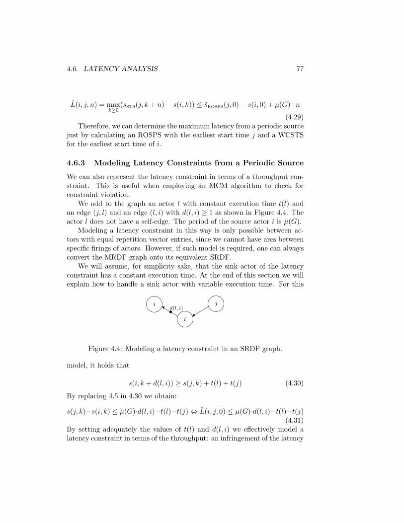
4.6. LATENCY ANALYSIS 77
L(i, j, n) = maxk≥0
(sSTS(j, k + n)− s(i, k)) ≤ sROSPS(j, 0)− s(i, 0) + µ(G) · n
(4.29)Therefore, we can determine the maximum latency from a periodic source
just by calculating an ROSPS with the earliest start time j and a WCSTSfor the earliest start time of i.
4.6.3 Modeling Latency Constraints from a Periodic Source
We can also represent the latency constraint in terms of a throughput con-straint. This is useful when employing an MCM algorithm to check forconstraint violation.
We add to the graph an actor l with constant execution time t(l) andan edge (j, l) and an edge (l, i) with d(l, i) ≥ 1 as shown in Figure 4.4. Theactor l does not have a self-edge. The period of the source actor i is µ(G).
Modeling a latency constraint in this way is only possible between ac-tors with equal repetition vector entries, since we cannot have arcs betweenspecific firings of actors. However, if such model is required, one can alwaysconvert the MRDF graph onto its equivalent SRDF.
We will assume, for simplicity sake, that the sink actor of the latencyconstraint has a constant execution time. At the end of this section we willexplain how to handle a sink actor with variable execution time. For this
j
l
id(l, i)
Figure 4.4: Modeling a latency constraint in an SRDF graph.
model, it holds that
s(i, k + d(l, i)) ≥ s(j, k) + t(l) + t(j) (4.30)
By replacing 4.5 in 4.30 we obtain:
s(j, k)−s(i, k) ≤ µ(G)·d(l, i)−t(l)−t(j) ⇔ L(i, j, 0) ≤ µ(G)·d(l, i)−t(l)−t(j)(4.31)
By setting adequately the values of t(l) and d(l, i) we effectively model alatency constraint in terms of the throughput: an infringement of the latency

78 CHAPTER 4. TEMPORAL ANALYSIS
constraint will be detected as an increase of µ(G), that is, an infringementof the minimum throughput constraint. The parameters can be set for anyvalues of d(l, i) and t(l) = µ · d(l, i)−L− t(j), as long as t(l), d(l, i) ≥ 0, butchoosing a low value for d(l, i) may constrain the pipelined execution of theiterations of the graph, for analysis purposes. Actor l and edges (j, l) and(l, i) do not need to have any equivalent in the implementation.
If j does not have a constant execution time, then we need one more newactor to model the latency constraint. Lets call this actor j′, with executiontime t(j′) = 0. All input arcs of j are redirected to j′. We then add adelay-less edge from j′ to j, and build the latency model as described abovewith j′ as the sink, instead of j.
4.6.4 Maximum Latency from a Sporadic Source
In reactive systems, it frequently happens that the source is not strictlyperiodic, but produces tokens sporadically, with a minimal time interval µbetween subsequent firings. Typically, a maximum latency constraint mustbe guaranteed. This will be the case, for instance, for the WLAN receiver wewill show in Chapter 5. It is easy to see that in such case, the MRDF graphhas to sustain a throughput of 1/µ in order to guarantee that it cannot beoverran by such a source, operating at its fastest rate. This means thatthe MCM of the graph, µ(G), is such that µ(G) ≤ µ. Our proof relies onthe possibility of bounding the self-timed behavior of a graph by a staticperiodic schedule with period µ, which is possible as long as µ(G) ≤ µ. Inthe following text, we will assume for simplicity, that µ(G) = µ, withoutloss of generality
In this section, we derive the maximum latency of an actor relatively toa sporadic source. First, we define a sporadic source more formally.
Definition 4.3. A source is sporadic if it fires with a forced schedule s′ suchthat s′(i, k) ≥ s′(i, k − 1) + µ.
Furthermore, we introduce a strictly periodic reference schedule s ofsource i with period µ, i.e.
s(i, k) = s(i, 0) + µ · k (4.32)
We define δ(k) asδ(k) = s′(i, k)− s(i, k), (4.33)
that is, delta is the difference between the actual time at which the sporadicsource has fired and the time at which our strictly periodic reference scheduleof source i fires.

4.6. LATENCY ANALYSIS 79
Lemma 4.1. If a source is sporadic then δ can only increase with everysubsequent iteration:
δ(k + 1) ≥ δ(k). (4.34)
Proof. We replace the definition of δ in 4.34:
(s′(i, k + 1)− s(i, k + 1))− (s′(i, k)− s(i, k)) ≥ 0. (4.35)
As s(i, k + 1) = s(i, k) + µ, Equation 4.35 becomes:
s′(i, k + 1)− s′(i, k) ≥ µ, (4.36)
which is true by hypothesis, since our source is sporadic.
Theorem 4.6. Consider an SRDF graph G = (V,E, t, d) and a schedules′ of that graph where all start times are self-timed, except for an externalsporadic source n whose forced schedule behaves according to Definition 4.3,with interval µ, and all execution times are worst case. Consider also theschedule s where the sporadic source is replaced by a periodic source s(i, k) =s(i, 0) + µ, with s(i, 0) = s′(i, 0), and where the firings of all other actorsare self-timed. Then, for all actors j ∈ V , it holds that:
s′(j, k) ≤ s(j, k) + δ(k − dd(n, j)). (4.37)
Proof. For any actor other than the source, all start times in both schedulesare self-timed. It therefore holds for any actor j ∈ V other than the sourcethat
s′(j, k) = max(x,j)∈V
(s′(x, k − d(x, j)) + t(x)) (4.38)
ands(j, k) = max
(x,j)∈V(s(x, k − d(x, j)) + t(x)) (4.39)
If we assume that the theorem applies to all the firings that precede the(j, k) firing, then s′(x, k) ≤ s(x, k) + δ(k − dd(n, x)), and it is true that
s′(j, k) ≤ max(x,j)∈V
(s(x, k − d(x, j)) + t(x) + δ(k − d(x, j)− dd(n, x))). (4.40)
Now, recall that dd(n, x) is the shortest path in delays from n to x. Throughthe triangle inequality of shortest paths [15], we know that
dd(n, x) + d(x, j) ≥ dd(n, j), (4.41)
80 CHAPTER 4. TEMPORAL ANALYSIS
for all x. Therefore, recalling Lemma 4.1, it is true that
δ(k − dd(n, x)− d(x, j) ≤ δ(k − dd(n, j)), (4.42)
and therefore
max(x,j)∈V
(s(x, k − d(x, j)) + t(x) + δ(k − d(x, j)− dd(n, x))) (4.43)
≤ max(x,j)∈V
(s(x, k − d(x, j)) + t(x) + δ(k − dd(n, j))).
Then, because of the inequality in Equation 4.40 we can write
s′(j, k) ≤ max(x,j)∈V
(s(x, k − d(x, j)) + t(x) + δ(k − dd(n, j))). (4.44)
and since δ(k− dd(n, j)) is constant inside the max expression we can yankit out to have
s′(j, k) ≤ max(x,j)∈V
(s(x, k − d(x, j)) + t(x)) + δ(k − dd(n, j)). (4.45)
Since s(j, k) = max(x,j)∈V (s(x, k − d(x, j) + t(x))
s′(j, k) ≤ s(j, k) + δ(k − dd(n, j)) (4.46)
We can now inspect the latency between an actor j and an external spo-radic source i, at an iteration distance of m. The definition of the maximumlatency is:
L(i, j, m) = maxk≥0
(s′(j, k + m)− s′(i, k)) (4.47)
It follows directly from Lemma 4.1 that maxp≤k δ(p) = δ(k). It follows fromTheorem 4.6 that:
s′(j, k + m) ≤ s(j, k + m) + δ(k + m− dd(i, j)) (4.48)
We know that the maximum start time in an STS is not later than theearliest possible start time in an SPS with period µ – which always exists,since µ(G) ≤ µ – thus
s(j, k + m) ≤ sµ(j, k + m) (4.49)
where sµ is a static periodic schedule of G with period µ.

4.6. LATENCY ANALYSIS 81
Given 4.49 and by definition of SPS, we can rewrite 4.48 in:
s′(j, k + m) ≤ sµ(j, 0) + µ · (k + m) + δ(k + m− dd(i, j)) (4.50)
Equation 4.47 implies that, it holds for all k ≥ 0 that
L(i, j, m) ≤ s′(j, k + m)− s′(i, k). (4.51)
Now, by replacing in this inequality the expressions we obtained for anupper and a lower bound, respectively, for s′(j, k + m) and s′(i, k):
L(i, j, m) ≤ sµ(j, 0) + µ · (k + m) + δ(k + m− dd(i, j))− s(i, 0)−µ · k− δ(k)
We then simplify the right-hand-side expression to obtain:
L(i, j, m) ≤ sµ(j, 0) + µ ·m + δ(k + m− dd(i, j))− s(i, 0)− δ(k) (4.52)
For m ≤ dd(i, j), since δ(k) ≥ δ(k + m− dd(i, j)), we can write:
L(i, j, m) ≤ sµ(j, 0)− s(i, 0) + µ ·m
The latency L(i, j, m) is not defined for m > dd(i, j) because the start timeof execution k + m of j is dependent on the start time of execution k + 1of i, which is unbounded, since the maximum difference between s(i, k + 1)and s(i, k) is undefined for a sporadic source.
When defined, the latency L(i, j, n) with a sporadic source has the sameupper bound as the latency for the same source, sink and iteration distancein the same graph with a periodic source with period µ.
4.6.5 Maximum Latency from a Bursty Source
We characterize a bursty source as a source that may fire at most n timeswithin any T time interval, with a minimal ∆t interval between consecutivefirings. A job that processes such a source must have µ(G) ≤ T/n to beable to guarantee its processing within bounded buffer space. Moreover, ifµ(G) ≤ ∆t, then we have the previous case, i.e., maximum latency from asporadic source. If µ(G) ≥ ∆t then latency may accumulate over iterations,as the job processes input tokens slower than the rate at which they arrive.The maximum latency must occur when the longest burst occurs, with theminimum interval between firings of the source, that is a burst of n tokenswith ∆t spacing. Because of monotonicity, making the source execute faster

82 CHAPTER 4. TEMPORAL ANALYSIS
T
µ(G)
source i′
source i
∆t
actor jL(i, j)
Figure 4.5: Arrival times of tokens of a bursty source relatively to strictlyperiodic source.
cannot make the sink execute slower, but it also cannot guarantee that itexecutes faster.
As depicted in Figure 4.5, the tokens of the bursty source i will arriveearlier than for the periodic source i′. Therefore, iteration n − 1 after thebeginning of the burst (iteration 0) happens the earliest time s(i, n − 1) =sROSPS(i, 0) + (n − 1) · ∆t. The firing n − 1 of j happens the latest ats(j, n−1) ≤ sROSPS(j, 0)+(n−1)·µ(G). Therefore, a bound on the maximumlatency is given by:
L(i, j, n) ≤ sROSPS(j, 0)− sROSPS(i, 0) + (n− 1)(µ(G)−∆t) (4.53)
4.7 Related Work
This chapter is an updated version of the work we previously presented in[73]. We are not aware of any other work on forced periodic sink behavior.
In [82], latency is defined as the time elapsed between periodic sourceand sink execution. This book also shows how this can be calculated by sym-bolic simulation of the worst-case self-timed schedule of the job graph. Thismethod requires symbolic simulation of the job graph, which is in generalintractable, even for Single Rate Data Flow graphs. Its definition of latencyis not as general as ours, since it only works if there is at least one delay-lesspath between source and sink. More importantly, it is only applicable ifthe external source is strictly periodic. In [25], a method is proposed formeasuring the minimal achievable latency of a self-timed implementation ofa MRDF graph. This work does not address the problem of bounding themaximum latency.

4.8. CONCLUSION 83
In [28], latency and buffer sizing are studied in the context of PGMgraphs, which are comparable in expressivity to MRDF graphs. The anal-ysis done in this work, however, limits itself to graphs with chain topology.Moreover, [28] does not allow for feedback loops, does not model inter-processor communication, requires EDF scheduling and a strictly periodicsource.
The event model used in the SYMTA/S tool [46] cannot cope with crit-ical cycles (i.e., they are not taken into account), and latency can only bemeasured as a result of a complete mapping, never taken into account as aconstraint during the mapping processes, as our analysis method allows.
There is recent work that confirms some of our results. In [22], a proof isgiven that a periodic linear bound exists on consecutive production times oftokens that occupy the positions of initial tokens for a MRDF graph. Theseare equivalent to the linear bounds that can be obtained with our method forthe firing times of the producers of such tokens. This paper also proposesa way of computing these bounds through a simulation-based technique.A comparison between our technique and this in terms of efficiency andtightness of the bounds could be interesting future work. In [92], the timinglinearity property is also shown to hold for Variable-Rate Data Flow.
4.8 Conclusion
In this chapter, we developed temporal analysis methods for static dataflow, that are derived from the monotonic property of MRDF graphs andespecially on the relation between self-timed and periodic schedules. Weuse this relation to reason not only about average throughput — to whichanalysis of self-timed schedules of MRDF graphs traditionally limits itself —but also about maximum latency and periodic behavior. These techniquesallow us to provide conservative linear bounds for all firings of actors of theMRDF graph — even during the transient phase of self-timed execution,and bound the effect of an increase of the worst-case execution time of anactor on the behavior of the graph.

84 CHAPTER 4. TEMPORAL ANALYSIS

Chapter 5
Compile Time Scheduling
In our approach to Software-Defined Radio, a radio transceiver is a concur-rent software program expressed by means of a data flow graph. In thischapter, we show how such a data flow graph can be partially scheduled atcompile time to a heterogeneous multiprocessor platform, in such a way thatguarantees of Hard Real-Time performance can be given. The schedulingdecisions taken at compile time are not complete, since, as already explainedin Chapter 2, the assignment of actors to processors in the physical plat-form must be done at runtime, to preserve the flexibility in the mappingthat allows for multiple instances of multiple transceivers to run simulta-neously. Nonetheless, we take as many scheduling decisions as possible atcompile time to decrease the complexity of the runtime mapping algorithmthat assigns hardware resources to each transceiver instance.
Accordingly, we take at compile time all the scheduling decisions thatrequire complex end-to-end temporal analysis of the graph. These includethe computation of buffer sizes, clustering of actors and static ordering ofactors per cluster, and the resource requirements towards the local runtimeschedulers of each processor.
Our strategy is to take the original actors of the data-flow graph andgroup them in clusters of statically-ordered actors. Each cluster will beassigned as one entity to one processor by the online processor allocationalgorithm. We then determine for each of these clusters the amount of pro-cessor resources, including scheduler settings for a Time Division Multiplex-ing (TDM) or a Non-Preemptive Non-Blocking Round Robin (NPNBRR)scheduler, and for all inter-cluster channels all buffer capacities, in such away that they are sufficient for the transceiver to meet its end-to-end HardReal-Time (HRT) requirements.
85

86 CHAPTER 5. COMPILE TIME SCHEDULING
We form clusters by mapping actors to virtual processors, and staticallyorder all the actors mapped to each given virtual processor. Each virtualprocessor represents a fragment of the resources of a physical processor inthe target platform. The designer must specify to the scheduler a targetplatform file containing a list of all virtual processors and their resources.We assume that all virtual processors of a given type can be mapped toa physical processor of the same type. For the sake of simplicity, we willassume that all physical processors of a given type have the same clockfrequency, and the same dynamic scheduler with the same settings.
We have shown in Chapter 3 and Chapter 4 that the self-timed executionof Single Rate Data Flow (SRDF) and Multi Rate Data Flow (MRDF) canbe analyzed for worst-case temporal behavior, assuming sufficient buffersizes. Our compile time scheduling algorithm requires the generation ofa data flow graph that models the temporal behavior of the input graphincluding the effects of each scheduling decision we take. Since schedulingdecisions can only decrease the throughput or increase the latency of thegraph execution, we can take decisions in incremental steps, and check,at each step, if each new decision still allows for a valid schedule. Wecan then exhaustively search the tree of scheduling decisions for solutions,backtracking each time an infeasible branch is found.
Our data flow scheduler is designed to schedule both single-rate (SRDF)and multi-rate (MRDF) graphs. MRDF graphs are first converted onto anSRDF equivalent, but special care must be taken to take into account thefact that multiple arcs in the converted graph correspond to a single bufferFIFO. For any actor in the input data flow graph that keeps state overconsecutive iterations (or equivalently has a self edge with unitary delay),we will require that the SRDF copies are mapped onto the same processor,to avoid state migration.
We will first explain how the scheduler works for input graphs that arealready single-rate (SRDF). We will then dedicate a section to explainingwhat must be changed in the scheduler to accommodate for graphs that wereoriginally multi-rate (MRDF). In Section 5.1 we will describe and providenotation for the inputs of our scheduler. In Section 5.2 we describe and pro-vide notation for the outputs of our scheduler. In Section 5.3, we will showhow the compile time scheduling decisions can be modeled conservatively bymeans of a data flow graph, and how a temporal model for a partial sched-ule of a graph can be constructed. After this, in Section 5.4 we motivatethe need for applying a combination of clustering and static ordering witha runtime scheduler. In Section 5.5 we define the compile time schedulingproblem and propose strategies to tackle it. In Section 5.6 we apply our

5.1. SCHEDULER INPUTS 87
techniques to obtain schedules for a TDS-CDMA receiver and a WLAN re-ceiver, that must share resources of a multi-processor platform. In Section5.7 we discuss related work and in Section 5.8 we state our conclusions forthis chapter.
5.1 Scheduler Inputs
Our scheduler requires three inputs: the task graph of the transceiver, adescription of the target platform onto which the transceiver is going tobe mapped, and a set of timing requirements. Furthermore, the user canoptionally specificy additional constraints to the mapping. In the followingsections we detail these inputs.
5.1.1 Target Platform
We model the hardware platform to which the application graph is going tobe mapped as a set of virtual processors. Each virtual processor representsa quantity of processing resources made available by the physical hardwareplatform. We chose to allocate resources of virtual processors at compiletime because this still allows the binding of virtual to physical processors tobe done at runtime, resulting in more mapping flexibility. Each virtual pro-cessor may represent all or a fraction of the resources of a physical processor.For example, we may map our application to a family of hardware platformsthat include two to four ARM processors. The virtual platform described asinput to the compile time scheduler can contain two (virtual) ARM proces-sors. At runtime, the resource manager may decide to allocate each of thevirtual processors to any two of the four physical processors, if the particularinstance of the hardware platform contains four ARM processors.
A virtual target platform is described by a set of virtual processors Π.The processors are described by a tuple (τ, sched, P, S). The valuation τ :Π → T , where T is the set of processor types, represents the type of theprocessor (for instances, an ARM or an EVP). The valuation sched : Π →tdm, rr, off represents the type of the dynamic scheduler that is runningon the processor. In the current implementation, this type can be tdm, ifthe processor implements a TDM scheduler, rr if the processor implementsa NPNBRR scheduler, or off, if the processor has no dynamic task schedulerrunning. The valuation P : Π → N0 represents the period of the scheduler(in a round-robin scheduler, this is the sum of the worst-case executiontimes of actors that can at any time be mapped onto the processor). Thevaluation S represents the maximum amount of processor resources that

88 CHAPTER 5. COMPILE TIME SCHEDULING
a single job can use per period. Therefore it must always hold that S ≤P . Furthermore, we assume that all processors of a given type have thesame value for sched and P , and we can therefore refer to the valuationssched : T → tdm, rr, off that, given a processor type, returns the type ofscheduler used in those processors, and valuation P : T → N0 that, given aprocessor type, returns the period of the scheduler for that type of processor.
One more observation about the relation between virtual processors andphysical processors is needed: two virtual processors can map onto a singlephysical processor during runtime mapping. If, for example, we have twovirtual processors with the same scheduler and period, and both with a max-imum utilization lower than half the period, the runtime resource allocatorwill always be able to map both virtual processors to the same physicalprocessor, if resources are available at the time of the allocation. By decid-ing how the target platform is described in terms of virtual processors tothe compile time scheduler, the designer can effectively control the clustergranularity.
5.1.2 Task Graph
A timed SRDF graph, annotated with processor type per actor and tokensize per arc, G = (V,E, d, t, τ, β) represents the data flow program thatcorresponds to a transceiver. V is the set of actors, E is the set of arcs. Eachactor in V corresponds to an invocation of a computational task in the inputLIME program. We call this graph the Task Graph of the application. Thet(i) valuation of actors corresponds to the WCETs of the computational taskinvocation on a specific processor type. We assume that each actor in thetask graph can only be mapped to a specific type of processor. The typeof processor on which a particular actor runs is given by an extra valuationτ : V → T . The valuation β : E → N0 represents the size β(i, j) in bytes ofeach token produced/consumed in arc (i, j) ∈ E.
5.1.3 Timing requirements
Input timing requirements are both throughput and latency constraints. Anactor i ∈ V may be required to have a minimal guaranteed throughput ofθ(i), and maximum latency requirements can be expressed as described inChapter 4. The throughput requirements are used to determine a requiredmaximum cycle mean µD for the graph. The maximum period has to besuch that all nodes meet their throughput requirement and therefore µD =mini∈V θ(i)−1. Latency constraints are expressed in the temporal analysis

5.1. SCHEDULER INPUTS 89
graph in terms of µD by using the latency modeling technique described inSection 4.6.3, on top of the temporal analysis model that will be describedin Section 5.3.
5.1.4 Additional Constraints
The scheduler accepts a number of additional mapping constraints. Thesewill not be discussed in the rest of this chapter, as adding verification of theseconstraints to the scheduler is conceptually straightforward, while includingthem in the remainder of the text will make all explanations and notationsmuch longer. These constraints are the following:
1. Memory space: besides cycles, actors consume memory space. De-pendent on the processor architecture, these may include several differ-ent memory pools, such as Instruction and Data Memory for Harvardarchitectures, or Instruction, X-Data and Y-Data for Dual-Harvardarchitectures. The data memories can be further subdivided in read-write, stack and read-only memories, for instances. Our scheduler al-lows for actors to be annotated with a vector of memory requirements,and virtual processors in the target architecture to be annotated with avector of memory provisions. Any valid schedule must respect that thesum of memory requirements of all actors mapped to a given processoris lower than the memory provided for each pool in that processor.
2. Forced Mapping: the designer can constrain the mapping of actorsto a specific processor in the virtual target platform.
3. Forced Co-mapping: the designer can instruct the scheduler to forcea set of actors in the task graph to be mapped to the same processor,i.e. the designer imposes that the set of actors belongs to the samecluster.
4. Forced Ordering: the designer may specify a order of executionbetween firings of two actors by adding an extra arc between them.
5. Buffer size restriction: the designer can instruct the scheduler toassume that the maximum buffer space between two actors is limitedby a given value. This will be further discussed in Section 5.3.2.

90 CHAPTER 5. COMPILE TIME SCHEDULING
5.2 Scheduler Output
The output of the compile time scheduler is given as a static order, a slicesize per processor, and a buffer capacity per edge in the input graph. Thestatic order is represented by the valuation so : Π → αn, where αn is theset of actor sequences of the type, [i1, i2, ...in], where i1, i2, ..., in ∈ V , andthe slice size for the cluster is given by valuation S : Π → N0. The staticorder also implies a processor allocation π : V → Π, such that, if, for agiven i ∈ V , if i ∈ so(p) =⇒ π(i) = p, meaning that actor i is mapped toprocessor p. In a complete compile time schedule, for any actor i ∈ V theremust exist a single processor p such that i ∈ so(p). The buffer capacity isrepresented by valuation b : E → N0, and represents the amount of tokensallocated to the edge.
5.3 Modeling Resource Allocation
In order to check whether a particular compile time schedule meets the tim-ing requirements, we generate a temporal analysis graph G′ that representsthe effects on the temporal behavior of graph G of the compile time scheduledescribed by (so, S). We must be able to conservatively model the effectsof actor ordering, local dynamic schedulers, communication channels andbuffer sizing. We will discuss first each one of these and then provide atransformation that, given the input data flow graph G, a target platform Πand a (partial) compile time schedule (so, S), generates the temporal anal-ysis graph G′(G, Π, so)
5.3.1 Communication channels
Depending on the target architecture and the level of detail required, com-munication channels between actors executing in different processors mightbe modeled in different ways. In [71] and [79] models are derived for theÆthereal network. Many different models for the same network are possible,depending on the level of abstraction. In the remainder of this chapter, wewill assume that communication between actors is done via remote storeswhose worst case time is accounted for in the execution times of the produc-ing actors. The reader is encouraged to consult [71] and [79] to find moreprecise and detailed models of communication. Any of these models is para-metric, depending on token size and the characteristics of the inter-processorcommunication hardware.
5.3. MODELING RESOURCE ALLOCATION 91
5.3.2 Buffer size restriction
A buffer capacity constraint can be modeled in an MRDF graph by addingto the input graph a back-edge from the consumer of a FIFO to its producerwith production/consumption rates that match the consumption/produc-tion rates of the forward edge. As the number of tokens in the cycle betweenproducer and consumer can never exceed the number of initial tokens in thatcycle, the edge that models the actual data FIFO can never have more thenthe number of tokens initially placed in the “credits” back edge plus thenumber of initial tokens in the forward edge. This also means that an ac-tor cannot fire without enough space being available in each of its outputFIFOs, which represents the worst-case effect of back pressure.
5.3.3 Task Scheduling
There are two types of task scheduling mechanisms that we are interestedin modeling: Compile Time and Runtime Scheduling.
Compile Time Scheduling (CTS) encompasses scheduling decisionsthat are fixed at compile time, such as static order scheduling.
Runtime Scheduling (RTS) refers to scheduling decisions that can-not be fully resolved at compile time, because they depend on the runtimetask-to-processor assignment, which in turn depends on the dynamic job-mix. This is handled by the local scheduling mechanism of the processor.Modeling the worst-case effect of the local scheduler on the execution of anactor is needed to include in the compile time analysis the effects of sharingprocessing resources among jobs. If the WCET of the task, the settings ofthe local dispatcher, and the amount of computing resources to be given tothe task are known, then the actor execution time can be set to reflect theworst-case response time of that task running in that local dispatcher,with that particular amount of allocated resources. In [7], we show how thiscan be computed for a TDM scheduler and, in [75], for a NPNBRR sched-uler. We will present these models in the following subsection and extendthem to handle its combination with static order scheduling.
5.3.4 TDM Scheduling
In [7], it has been shown that the effect of TDM scheduling can be modeledby replacing the worst-case execution time of the actor by its worst-caseresponse time under TDM scheduling. The response time of an actor i isthe total time it takes to fire i , when resource arbitration effects (scheduling,preemption, etc) are taken into account. This is counted from the moment

92 CHAPTER 5. COMPILE TIME SCHEDULING
the actor meets its enabling conditions to the moment the firing is completed.Assuming that a TDM wheel period P is implemented on the processor andthat a time slice with duration S is allocated for the firing of i, such thatS ≤ P , a time interval equal or longer than t(i) passes from the moment anactor is enabled by the availability of enough input tokens to the completionof its firing. This is due to what can be seen as two different effects of TDMarbitration. The first of this is the arbitration time, i.e. the time it takesuntil the TDM scheduler grants execution resources to the actor, once thefiring conditions of the actor are met. In the worst-case, i gets enabled whenits time slice has just ended, which means that the arbitration time is thetime it takes for the slice of i to start again. If we denote the worst-casearbitration time as rA then:
rA(i) = P − S. (5.1)
The second effect has to do with the fact that the time slice may be toosmall for the firing of i to be executed in a single slice. We shall call the timebetween the moment that the actor starts execution and finishes executionthe processing time of the actor, and denote it by rP . The time i willtake to fire, in the worst-case, is equal to
rP (i) = b t(i)Sc · P + (t(i) mod S). (5.2)
Since t(i)modS = t(i) − S.b t(i)S c, the previous expression can be re-written
as:rP (i) = b t(i)
Sc · (P − S) + t(i). (5.3)
The total worst-case response time of i is then given by the sum of thesetwo values:
r(i) = rA(i) + rP (i) = (P − S) · (b t(i)Sc+ 1) + t(i) (5.4)
By replacing the t(i)s of all actors scheduled under TDM by their worst-case response times, r(i)s, temporal analysis of the timed SRDF graph thusobtained will yield the minimum guaranteed throughput that is attainableby such an implementation.
In later work [92] it was shown that a more accurate model of a TDMscheduler can be built by modeling by a generic data flow model for a latency-rate server [84]. The effect on the timing of an actor i with execution timet(i) of executing it under a latency-rate server can be modeled in data flow

5.3. MODELING RESOURCE ALLOCATION 93
by replacing the actor by two actors: an actor iL and an actor iR. All theinput edges of actor i are connected as inputs to iL, and all output edges ofactor i are connected as outputs to the rate actor iR. Furthermore, an edge(iL, iR) with no delays and an edge (iR, iR) with one delay are added to thegraph. The execution times of the actors in the model are given by
t(iL) = P − S (5.5)
and
t(iR) = P.t(i)S
. (5.6)
5.3.5 NPNBRR Scheduling
In a Non-Preemptive Non-Blocking Round-Robin (NPNBRR) Scheduler, allclusters assigned to the same processor are put in a circular scheduling list.The runtime scheduler goes through this list continuously. It picks an actorfrom the list and tries to execute it. The actor (or the scheduler, dependingon the implementation) checks for input data and output space availability.If there are sufficient input data tokens available in all input FIFOs andoutput space available in all output FIFOs such that the actor can consumeand produce tokens according to its firing rules, the actor executes until thefiring is over, if not, the actor is skipped. The process is repeated for thenext actor in the circular scheduling list, and so on.
The worst-case arbitration time of an actor is given by the sum of theexecution times of all other actors mapped to the same NPNBRR-scheduledprocessor. The processing time is equal to the actor’s execution time, sincethere is no preemption. The total response time is therefore equal to thesum of the execution times of all actors mapped to the NPNBRR-scheduledprocessor.
As for the representation of scheduler settings for an NPNBRR scheduler,we will take the maximum allowed sum of worst-case execution times oftasks per turn of the Round-Robin wheel as the chosen maximum periodP and the maximum sum of worst-case execution times for a given clusterof statically-ordered actors as the maximum slice S(p) of the resources ofprocessor p by a task graph G.
5.3.6 Static Order Scheduling
A static order schedule of a set of actors A = a0, a1, ..., an mapped to thesame processor is a sequence of execution so = [ak, al...am] that generates

94 CHAPTER 5. COMPILE TIME SCHEDULING
extra precedence constraints between the actors in A such that from thestart of the execution of the graph, ak must be the first to execute, followedby al and so on, up to am. After am executes, the execution restarts fromak for the next iteration of the graph.
Any static order imposed to a group of SRDF actors executing on thesame processor can be represented by adding edges with no tokens betweenthem. From the last to the first actor in the static order an edge is alsoadded, with a single initial token. This construct reflects the fact that, thegraph execution being iterative, when the static order finishes execution fora given iteration, it re-starts it from the first actor in the static order forthe next iteration.
Notice that the new edges represent a series of sequence constraints en-forced by the static order schedule and do not represent any real exchangeof data between the actors. In the data flow diagrams that follow, for easeof reading, every time there is more than one edge from the same source tosink, only one edge with the lowest d(i, j) is represented, as it imposes thetightest sequence constraint between the actors.
5.3.7 Combining Static Order and TDM
Let’s assume that instead of attributing a separate TDM slice to each actorwe attribute a single TDM slice to a group of actors and we statically orderthese actors. The reasons why we may want to do this are exposed insection 5.4. For now we will focus only on how such a mixed schedule canbe modeled for the purpose of worst-case analysis.
Consider a set of actors a1, a2, a3, belonging to the same job, andmapped to the same processor p. Consider that a static order of executionso = [a1, a2, a3] has been imposed on them, and that this static order exe-cution is allocated to a time slice of S time units within a time wheel witha period P .
Since the actors are guaranteed to be mutually exclusive because of thestatic order, it turns out that whenever one of them is activated none ofthe remaining others is. Thus, we can conservatively assume that the TDMscheduling will affect the timing of executing each actor in the same way asit would if the time slice were allocated exclusively to it. We can thereforemodel the combined effect of the static order and TDM scheduler by addingto the scheduling analysis graph the edges that represent the imposed staticorder and replacing each actor by the latency-rate model of its executionunder a budget scheduler, as described in section 5.3.4. This is depicted inFigure 5.1 for three actors a1,a2 and a3, statically ordered and assigned a

5.3. MODELING RESOURCE ALLOCATION 95
slice with time S.
a1R
a2R
a1L
a2L
c
d
a1
a2
c
d
a3e a3Ra3Le
Figure 5.1: Modeling the combined effect of static order and TDM schedul-ing
5.3.8 Mixing Static Order and NPNBRR scheduling
Modeling the effect on timing of NPNBRR scheduling over a cluster ofstatically-ordered actors is somewhat similar to the previous case. The maindifference is that each actor will run to completion once its input is available,without being preempted by the scheduler.
Consider C = a1, a2...an, a set of actors belonging to the same jobG, and mapped to the same processor p. Consider that a static order ofexecution so = [a1, a2, ...an] has been imposed on them, and that the totalsum of execution times of actors in the Round-Robin list of processor p is P .This includes the actors belonging to this cluster and any other clusters thatthe runtime resource manager has allocated to the same processor. Underthese conditions, the first actor in the cluster, a1, will be able to fire for thefirst time, in the worst case, after the time at which its first input tokenhas been produced plus an arbitration time equal to P −
∑an∈C t(an). This
time may be used by actors from other jobs running on the same physicalprocessor. Note that actors belonging to the same cluster as a1 are notaccounted for here, since those dependencies are modeled with edges inthe graph, and enforce mutual exclusivity. After a1 finishes firing, a2 canimmediately fire if input data is available. If not, the firing will be delayed,and the Round Robin scheduler moves to the next cluster. Once an inputtoken has become available, the NPNBRR can take, at most a time equalto P −
∑an∈C t(an) to allow a2 to fire. The same is true for a3 and all

96 CHAPTER 5. COMPILE TIME SCHEDULING
other actors in the cluster. This effect can be modeled by introducing inthe analysis model, for each actor ai ∈ C, a latency actor aiL with t(aiL) =P −
∑an∈C t(an), adding edges (aiL, ai), with d(aiL, ai) = 0, and further
replacing all edges in the set (j, ai) ∈ E : ai ∈ C, j /∈ C, by edges (j, aiL)each with the same delay as the corresponding (j, ai).
Since each actor in the static order is still limited to execute at most onceper period, it occurs that in the worst case, after the last actor has executed,the first can only execute again after a time interval of P −
∑an∈C t(an) has
elapsed, even if input tokens are readily available. This can be modeledby adding an actor with execution time P −
∑an∈C t(an) at the end of the
cluster. Figure 5.2 depicts the conversion to the analysis model for a clusterof three statically ordered actors a1, a2 and a3.
a1R
a2R
a1L
a2L vp
c
d
a1
a2
c
d
a3e a3Ra3Le
Figure 5.2: Modeling the combination of static order and NPNBRR
5.3.9 Temporal Analysis Model
Having defined how to model the effects of our compile time schedulingdecisions on an SRDF graph, we are ready to present a graph transformationthat allows us to obtain a temporal analysis model SRDF graph G′, fromthe knowledge of the original task graph G, the target platform Π, and thecompile time schedule (so,S).
We first define the set of edges in G internal to virtual processors:
Eint = (i, j) ∈ E | π(i) = π(j), (5.7)
and the set of edges between virtual processors
Eext = (i, j) ∈ E | π(i) 6= π(j) = E − Eint. (5.8)

5.3. MODELING RESOURCE ALLOCATION 97
The reason why we separate the treatment of external and internal edges isthat we do not need to assume that internal edges must wait for the latencyterm in the response model, as both producer and consumer actors mustbelong to the same cluster, and their dependencies are already modeled inthe graph. The analysis model G′(G, Π, so, S, P ) = (V ′, E′, t′, d′) is thengiven by replacing all actors in G for their latency-rate models as describedabove, adding edges to represent the static ordering, and computing theexecution times of these new nodes:
V ′ = iL | i ∈ V ∪ iR | i ∈ V ∪ vp | p ∈ Π;E′ = (iL, iR) | i ∈ V ∪ (iR, iR) | i ∈ V ∪ (iR, jR) | (i, j) ∈ Eint ∪ (iR, jL) | (i, j) ∈ Eext∪ ∪p∈Π∧so(p)=[i1,i2,...,in](i1R, i2R), (i2R, i3R), ...,
(i(n−1)R, inR), (inR, vp), (vp, i1R);d′ = ∪i∈V ((iL, iR), 0), ((iR, iR), 1)∪ ∪(i,j)∈Eint
((iR, jR), d(i, j))∪ ∪(i,j)∈Eext
((iR, jL), d(i, j))∪ ∪p∈Π∧so(p)=[i1,i2,...,in]((i1R, i2R), 0), ((i2R, i3R), 0), ...,
((i(n−1)R, inR), 0), ((in, vp), 0), ((vp, i1), 1);t′ = (iL, lat(i)) | i ∈ V ∪ (iR, rat(i) | i ∈ V ∪ (vp, pro(p) | p ∈ Π
where the functions lat, rat and pro are given, respectively, by
lat(i) =
P (π(i))− S(G, π(i)) if sched(π(i)) = tdmP (π(i))− S(G, π(i)) if sched(π(i)) = rr0 if sched(π(i)) = off
rat(i) =
P (π(i)).t(i)S(G,π(i)) if sched(π(i)) = tdm
t(i) if sched(π(i)) = rrt(i) if sched(π(i)) = off
pro(p) =
0 if sched(π(i)) = tdmP (π(i))− S(G, π(i)) if sched(π(i)) = rr0 if sched(π(i)) = off
where we simply used the formulas for the two terms of the latency ratemodels for TDM and NPNBRR schedulers.

98 CHAPTER 5. COMPILE TIME SCHEDULING
5.3.10 Temporal Analysis Model for Partial Schedules
The construction of the temporal analysis model as given in the previoussection assumes that the whole graph has been scheduled onto the targetplatform. During scheduling, we will need to check whether a partial sched-ule is feasible or not. In partial schedules, some actors may not yet have beenmapped and the size of slices S(p, G) allocated to the graph on a specificprocessor may not be yet known.
Our strategy when analyzing the temporal behavior of a partial sched-ule is to always take the most optimistic assumption about the overheadcaused by the mapping of any actor that has not yet been yet assigned to aprocessor, with the objective of not excluding any feasible complete solutiona priori. Sometimes, a particular combination of optimistic assumptions isclearly not feasible in practice. Say that actor B, which is yet unmapped,communicates both with actor A and actor C, which are respectively mappedto processor 1 and 2. Furthermore, A, B and C all map to the same pro-cessor type. We will assume that B communicates without inter-processoroverhead with both A and C, although it is patent that, once mapped, Bcan be mapped to processor 1 or to processor 2, but not both. The rea-son for taking always optimistic assumptions for partial schedules, is thatour scheduler, which we will present in detail in Section 5.5, searches forfeasible schedules by assigning actors to processors one by one, and check-ing at each assignment whether the cumulative set of assignment decisionshas not created an infeasibility. Taking pessimistic assumptions about un-mapped actors would leads us to potentially exclude feasible schedules fromthe search.
If the processor allocation of an actor i ∈ V is known, and the slice sizeS(π(i), G) has not yet been determined, then we make the slice size equal tothe maximum slice S(π(i)), since the final slice can never exceed that value,in the computation of the functions rat and lat.
As for an actor i ∈ V yet unmapped, the π(i) is undefined, which wewill denote by π(i) = ⊥. We must redefine the analysis model for this case.Edges where one of the endpoint actors is still unmapped are consideredinternal edges, if the processor type of the two is the same, and externalif the processor type is different (independently of what mapping eventu-ally is chosen, it is guaranteed that the two actors will not be in the sameprocessor). Therefore, in generating a temporal analysis model for a partial

5.3. MODELING RESOURCE ALLOCATION 99
schedule, the sets Eint and Eext are given by
Eint = (i, j) | (i, j) ∈ E ∧ (π(i) = π(j) ∧ π(i) 6= ⊥)∪ (i, j) | (i, j) ∈ E ∧ (π(i) = ⊥ ∨ π(j) = ⊥) ∧ τ(i) = τ(j);
Eext = E − Eint.
Furthermore, we must define the values of lat and rat for unmapped actors.In the best case, an actor i ∈ V for which π(i) = ⊥ will be mapped to theprocessor of type τ(i) that offers the highest maximum slice size, that is,in this case, we make S(π(i), G) = maxp∈Π∧τ(p)=τ(i) S(p) in the equationsfor lat and rat. This is possible since we assume that all processors of thesame type have the same dynamic scheduler settings (i.e. scheduler typeand period).
As an example, we depict in Figure 5.3 a data flow graph representingthe application(on the left) and its analysis model (on the right). The inputgraph has 4 actors a, b, c and d. The processor types to each this actorsmap are τ(a) = τ(c) = ARM and τ(b) = τ(d) = EV P , that is a and crun on ARM processors, whereas b and d run on EVP processors. Further-more, we are mapping this application to a virtual platform that includesseveral ARMs and EVPs. One of the ARMs is named ARM1 and one ofthe EVPs is EVP1. Assume that the current partial schedule includes onlymappings to these two processors, and it is the following: the static orderfor ARM1 is so(ARM1) = [a, c], and, for EVP1, is so(EV P1) = [b]. Sinceeach processor runs a scheduler (for the topology it does not matter whetherit is TDM or NPNBRR), we insert a latency-rate model for each actor. Weadd edges (aR, cR), and edges (cR, vARM1) and (vARM1, a), to represent thestatic order. The processor actor is required to accurately model the budgetreplenishment interval for NPNBRR, and its execution times is 0 for a TDMscheduler. Application edges between actors mapped to different processors(such as (a, b)), or between actors mapped to different processor types (suchas (c, d) are represented in the model by edges between the R actor of theproducer and the L actor of the consumer. An application edge betweenactors mapped to the same processor, or, alternatively, having the sameprocessor type, where at least one of the actors has not been mapped yet(such as (b, d)), are represented in the model by an edge from the R actor ofthe producer to the R actor of the consumer, since it may still be possiblefor the two to be mapped to the same processor.

100 CHAPTER 5. COMPILE TIME SCHEDULING
aR
cR
aL
cL
vARM1a
b
dbRbL
c
vEVP1dRdL
Figure 5.3: Example of the generation of an analysis model for a partiallyscheduled graph.
5.4 Why we combine CTS and RTS
Although static order scheduling is a popular strategy for scheduling dataflow graphs [82], it cannot singly solve our mapping problem. Since jobs startand stop independently, a static order schedule would have to be computedat design time for every combination of jobs that can be active simultane-ously. This problem is aggravated by the fact that, when a transition occursfrom a job-mix to another, remaining jobs must not experience any discon-tinuity caused by the change of configuration. Secondly, as different jobscan have very different rates, a static schedule could only be realized if thefaster jobs where almost completely latency-insensitive, which is certainlynot the case with jobs such as Wireless LAN and, even if this were the case,the length of the static order schedule and the amount of buffering of inputsrequired could easily become prohibitive.
One could think of simply using local TDM or NPNBRR schedulers perprocessor and relying on FIFO communication for actor synchronization.The main problem with such a strategy is that the bounds on the worst-case response times of actors executing on independent slices completelyoverlook the fact that, within a job, we have more information about theinterdependence of actors. For instances, a set of actors may be mutuallyexclusive – in an SRDF graph this happens when the actors belong to the
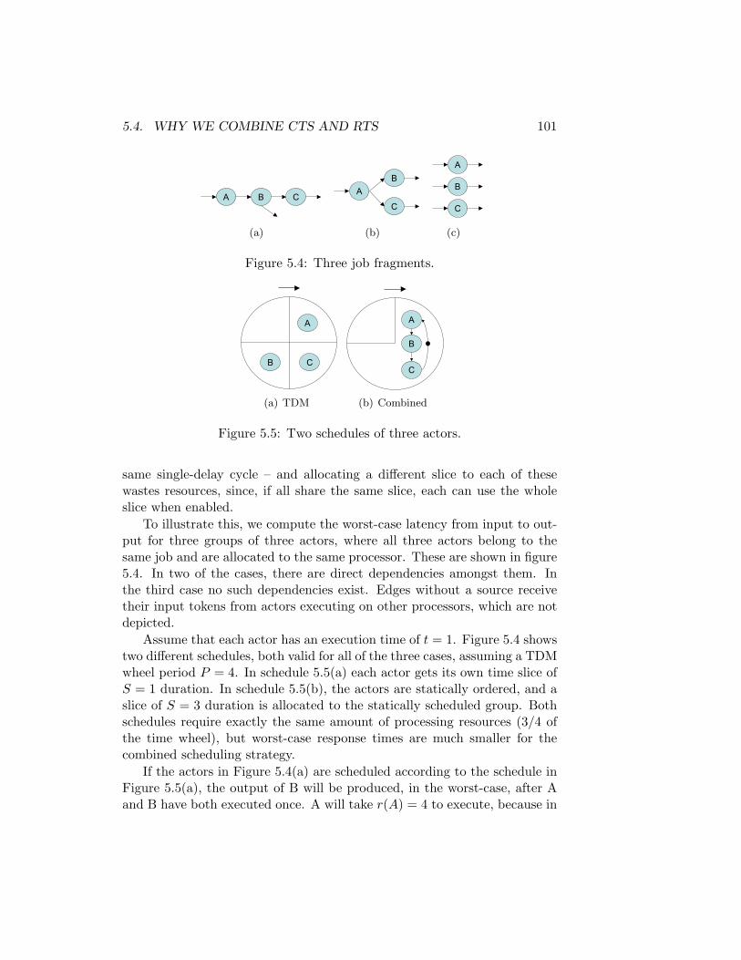
5.4. WHY WE COMBINE CTS AND RTS 101
A CB
A
B C
A
C
B
A
B
C
(a)
A CB
A
B C
A
C
B
A
B
C
(b)
A CB
A
B C
A
C
B
A
B
C
(c)
Figure 5.4: Three job fragments.A CB
A
B C
A
C
B
A
B
C
(a) TDM
A
C
B
(b) Combined
Figure 5.5: Two schedules of three actors.
same single-delay cycle – and allocating a different slice to each of thesewastes resources, since, if all share the same slice, each can use the wholeslice when enabled.
To illustrate this, we compute the worst-case latency from input to out-put for three groups of three actors, where all three actors belong to thesame job and are allocated to the same processor. These are shown in figure5.4. In two of the cases, there are direct dependencies amongst them. Inthe third case no such dependencies exist. Edges without a source receivetheir input tokens from actors executing on other processors, which are notdepicted.
Assume that each actor has an execution time of t = 1. Figure 5.4 showstwo different schedules, both valid for all of the three cases, assuming a TDMwheel period P = 4. In schedule 5.5(a) each actor gets its own time slice ofS = 1 duration. In schedule 5.5(b), the actors are statically ordered, and aslice of S = 3 duration is allocated to the statically scheduled group. Bothschedules require exactly the same amount of processing resources (3/4 ofthe time wheel), but worst-case response times are much smaller for thecombined scheduling strategy.
If the actors in Figure 5.4(a) are scheduled according to the schedule inFigure 5.5(a), the output of B will be produced, in the worst-case, after Aand B have both executed once. A will take r(A) = 4 to execute, because in

102 CHAPTER 5. COMPILE TIME SCHEDULING
TDM Comb.Job a Job b Job c All
Out A 4 4 4 2Out B 7 7 4 3Out C 10 7 4 4
Table 5.1: TDM vs Combined scheduling.
the worst-case A has to wait for 3/4 of the wheel to turn to get its slice, andthen take 1/4 of the wheel to process. Now B has to execute once. Thattakes r(B) = 4 − 1, since B can execute sooner that waiting for a full turnafter A has completed – we know that B is not allocated to the same slice asA. The output of B will therefore be generated after r(A) + r(B) = 7 unitsof time. The output of C will still have to wait for the response time of C,which will be again less than one period, since the slice allocated to C willcertainly be reached before the slice of B, which just finished. Thereforer(C) = 3, and C will produce output after r(A) + r(B) + r(C) = 10 timeunits. On the other hand, the combined TDM/static order schedule 5.5(b)takes as worst-case the time from the end of the slice allocated to the groupto the next end of the slice allocated to the group, since the 3 actors allexecute in sequence within one slice. Therefore, A ends execution at time2, the output in B is produced at time 3 and the output of C has a responsetime of 4.
For job 5.4(b), the TDM schedule in figure 5.5(a) will yield a responsetime of 4 + 3 = 7 for both external outputs, while the combined schedulewill yield the same values as for job 5.4(a).
For job 5.4(c), the combined schedule imposes an arbitrary order be-tween 3 independent actors, and thus creates extra scheduling dependencies.However, the worst-case production times, assuming all external inputs areavailable, are still 2, 3, 4, for the outputs of A, B and C, respectively, whilefor the TDM schedule, the worst-case production times are 4, 4, 4. Notehowever that in this case the combined schedule imposes an extra depen-dency on the arrival of the input of A to the production of B’s output,which did not exist before. If the input of B is ready before the input of A,this particular schedule may be quite inefficient. However, this is a prob-lem of choosing the “right” static order. The results of this example aresummarized in Table 5.1.
The point we want to make is that the combination of TDM with staticorder schedule allows, when applicable, the determination of much tighter

5.5. THE SCHEDULING PROBLEM 103
bounds on worst-case response times for the same amount of allocated re-sources than TDM. A similar example could be given for NPNBRR sched-ulers. Since at compile time we know only about one single job, it is at thislevel that static order can be used to shorten worst-case bounds on responsetimes.
Because of this, we use different scheduling methods to schedule amongtasks within a job (intra-job scheduling) and to reserve resources amongjobs (inter-job scheduling) such that each running job can meet its timingrequirements independently of any starts/stops of other jobs.
Intra-job scheduling is handled by means of static order, i.e., per joband per processor, a static ordering of actors is found that respects the Real-Time requirements while trying to minimize processor usage, while inter-jobscheduling is handled by means of local TDM/NPNBRR schedulers. In thecase of TDM, scheduling, per job and per cluster of statically-ordered actors,a slice time with duration S must be determined.
An admission controller is needed to start jobs upon the arrival of a startrequest. It is similar to the one we suggested in [74], in that it must check ifenough memory, communication and computing resources (enough time inthe TDM wheel of the processor) are available for the requirements of thejob. If not, the start of the job is refused. The mapping algorithms used bythe admission controller are described in detail in Chapter 7.
5.5 The Scheduling Problem
Our objective is to schedule each job in such a way that we guarantee real-time constraints and minimize processing resource usage, such that resourcescan be shared with other running jobs, both increasing the probability ofstarting the job on an already running system, and the probability thatjobs requested to start later will find enough resources to start. We needto define the period P (p) of the time wheel on each processor p ∈ Π , theslice time S(p, G) attributed to job G on processor p, a static order scheduleso(p, G) per processor p and job G and sizes for all buffers. The maximumacceptable period between consecutive executions of an SRDF actor for agiven job graph G is given by µD.
In order to propose a solution for this problem, we must first discussoptimization criteria. After this, we will discuss how to decouple differentdecisions in the scheduler, and we will then describe our proposed solutionsfor each phase.

104 CHAPTER 5. COMPILE TIME SCHEDULING
5.5.1 Optimization Criteria
For each job, the schedule should use as few cycles per period as possible,as this will increase the percentage of the processor available to other jobs.A good measure of the amount of processing resources used by a job G ona processor p is the processor utilization U(p, G), which can be defined, forTDM, as the ratio between the time reserved on the processor for the joband the total number of cycles per time wheel period:
U(p, G) =S(p, G)P (p)
. (5.9)
The processor period P (p) is, as we have seen, defined per processor asa fixed system parameter which is considered an input by the scheduler.We will discuss in Section 5.5.3 how to appropriately chose the value of thisparameter.
For a heterogeneous multiprocessor, we try to reduce the utilization of allprocessors. This is done in a weighted way, since it is possible that certainprocessors types are in general more required than others, and thus theirutilization should be kept lower. We introduce a processor cost coefficientc(p).
Our optimization criterion is the minimization of the weighted sum ofthe utilizations:
minimize∑p∈Π
U(p, G) · c(p) (5.10)
This function still disregards the fact that, although the resources ofa processor may be scarcer than of another, if the ”cheaper” processor isfully occupied, several jobs may become impossible to start – e.g. a sec-ond instance of an already running job. This could be accounted for byan optimization criterion that makes the cost of a processor increase withutilization, but that would yield a complex, non-linear objective function.Instead, we rely on defining our maximum slice size per job, S(p) per pro-cessor as part of the input to the scheduler, and enforcing that S(p, G) mustbe kept lower than S(p) for any valid schedule.
Another potentially important optimization criterion is the amount ofbuffering required in total and by processor. In our work we decided toassume that buffering was less important than processor utilization. This isbecause in the radio models that we studied buffer sizes were typically smalland mostly independent from the other resource allocation decisions, as weshall see in the results section.

5.5. THE SCHEDULING PROBLEM 105
5.5.2 Phase decoupling
The problem of trying to find P (p), S(p, G) , so(p, G), and b(i, j), subject tothe afore-mentioned constraints and optimization criterion is complex. It istherefore necessary, when designing the scheduler, to try to define a numberof phases in which each of the decisions is taken.
The choice of the periods of the schedulers, P (p), should be independentof the actual jobs, and these values should simply be given as inputs to thescheduler. Nonetheless, the choice of periods is a very important decision,and one that can be made much easier by taking into account the charac-teristics of the transceivers that one knows will be required to run in theplatform. Section 5.5.3 discusses how to chose these values.
For NPNBRR schedulers, the choice of S(p, G) is made along the choiceof so(P,G). This is because, for a NPNBRR scheduler, since preemptionis not possible, the slice sizes are simply equal to the execution times ofthe tasks allocated to the processor. For TDM schedulers, we have an extraphase of the compiler dedicated to trying to reduce the size of the slices, aftera feasible so(P,G) has been found. A third phase takes care of computingfeasible buffer sizes for all FIFOs, and can be applied before, after or in-between the two other phases, depending on how many buffering resourcesare available in the platform.
5.5.3 Determining Scheduler Settings
For an NPNBRR scheduler, we do not have many options in the choice ofthe period P (p) of processors. Say that we want to be able to run a numberof different jobs, each with a different µD. Since for the lowest µD it isstill required that each actor fires once per period, we should set P (p) atmost to the value of the lowest µD across all the jobs we intend to mapin the platform. This value is likely to make other jobs unschedulable, ifthey are composed of actors, with execution times too high to fit in a singleturn of the Round Robin wheel. In such a case, one can consider that whensuch a job is running, there can be no sharing of resources with the fasterjob, and the compile time scheduling can be carried out with a higher µD.This will, however, make it impossible for this job to share resources withany job with a faster µD for that processor type. Also, since one of ourgiven requirements (see Chapter 2), is that we cannot know at compile timeall other transceivers that may be mapped in the platform, our choice ofP (p) can only be based on the jobs that are known at design time, and onknown characteristics (such as sampling rates) of transceivers that may in

106 CHAPTER 5. COMPILE TIME SCHEDULING
the future be added to our platform.For TDM schedulers, assuming a constant processor utilization, we no-
tice by inspecting Equation 5.4 that when the time wheel period decreases,the worst-case response time of an actor becomes closer to its executiontime. This suggests that the processor period of a TDM scheduler shouldbe as small as possible, while still allowing partitioning of processing re-sources among the maximum amount of job instances one wishes the plat-form to be able to run simultaneously. However, this neglects the overheadcaused by the context-switching time at the change of time slice: since thecontext-switching time is constant, a smaller time wheel period implies ahigher absolute number of context switches and, thus, a lower utilization ofthe processors. We can chose P (p) in such a way that we guarantee thatthe overhead of context-switching does not exceed an arbitrary percentagepcc(p) of the processing cycles of p. If cc(p) is the cost of a context-switchfor processor p and nj(p) is the maximum number of job instances we wishto run simultaneously, and since per each period each job gets one timeslice, then the number of cycles per period spent on context switching iscc(p) · nj(p) and the value of P (p) should be set such that:
P (p) ≥ cc(p) · nj(p)pcc(p)
(5.11)
On the other hand, since any actor in a timed SRDF graph must beable to execute once per µD of its job to meet the temporal constraints, thetime wheel period must be such that allows this for all jobs, and thereforeP (p) ≤ µD(G) for any job G the system must run. If the two inequalities arenot compatible, one must accept a higher percentage of context-switchingoverhead.
5.5.4 Finding Static Order Schedules
Our data flow scheduler groups actors into clusters, while simultaneouslyordering actors statically within each cluster.
The first thing to notice about the static order schedules is that theonly precedence constraints that need to be respected are the ones insideone iteration. This is because the static order imposes an execution orderwith no iteration overlap per cluster (but notice that between two differentclusters there may still be iteration overlap). Therefore, for the purpose ofthe static order schedule, only edges in the input graph that have the delayequal to 0 need to be taken into account.

5.5. THE SCHEDULING PROBLEM 107
To give an idea of how the static order of actors on a processor influencesthe temporal behavior, we will give an example. Figure 5.6 depicts the timedSRDF model of a job. Assume that actors A, B and C are allocated to acluster and D to another. Assume also that t(A) = t(B) = t(C) = t(D) = 1and that µD = 3. The MCM of the job is µ = 3, because of the ACD cycle.
Now inspect the two clustered static order schedules in Figure 5.7. Bothof them respect the precedence constraints defined by the 0-delay edges, butwhile the schedule depicted in 5.7(a) has an MCM of 3, from cycles ACDand ACB, the schedule depicted in 5.7(b) exceeds µD since the cycle ABCDhas µc = 4, due to the extra dependency caused by the static order on thefirst cluster.
A
B C D
A
B
C D
A
C
B
DP1
P2
P2
P1
Figure 5.6: A job.
The data flow scheduler works thus: first, a Direct Acyclic Graph (DAG)representing the dependencies between actors within an iteration is gener-ated, by removing all edges with delays from the input graph. Then thescheduler starts. It picks an actor without dependencies. It generates a listof processors to which the selected actor can be mapped. It then selectsone of these processors, and tries to map the selected actor to the selectedprocessor. This appends the actor to the statically-ordered sequence of agiven processor.
After each mapping attempt decision, a temporal analysis model for theobtained partial schedule is constructed, and an MCM computation checkswhether the MCM of the temporal analysis model is lower than the requiredµD. For MCM computation, we implemented the Howard algorithm [13],since it is one of the fastest, according to the benchmark provided in [17]and, being a policy-improvement algorithm, it is easy to write an incrementalversion of it: at each step we can start the search of the MCM for the newmodel graph by the MCM cycle which was the solution in the previous step.
If the MCM of the temporal analysis model is below µD the last schedul-ing decision is kept, the DAG is updated by removing the actor that wasmapped, a new actor the is considered from the fireable nodes in the DAG. If
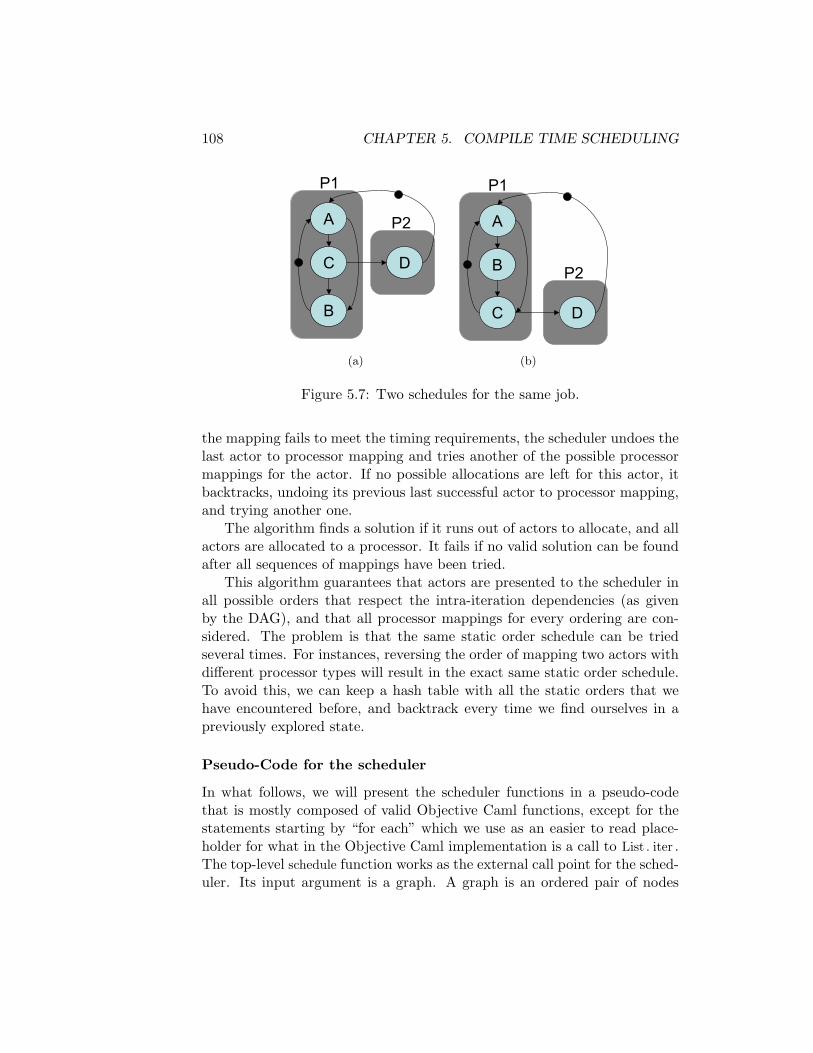
108 CHAPTER 5. COMPILE TIME SCHEDULING
A
B C D
A
B
C D
A
C
B
DP1
P2
P2
P1
(a)
A
B C D
A
B
C D
A
C
B
DP1
P2
P2
P1
(b)
Figure 5.7: Two schedules for the same job.
the mapping fails to meet the timing requirements, the scheduler undoes thelast actor to processor mapping and tries another of the possible processormappings for the actor. If no possible allocations are left for this actor, itbacktracks, undoing its previous last successful actor to processor mapping,and trying another one.
The algorithm finds a solution if it runs out of actors to allocate, and allactors are allocated to a processor. It fails if no valid solution can be foundafter all sequences of mappings have been tried.
This algorithm guarantees that actors are presented to the scheduler inall possible orders that respect the intra-iteration dependencies (as givenby the DAG), and that all processor mappings for every ordering are con-sidered. The problem is that the same static order schedule can be triedseveral times. For instances, reversing the order of mapping two actors withdifferent processor types will result in the exact same static order schedule.To avoid this, we can keep a hash table with all the static orders that wehave encountered before, and backtrack every time we find ourselves in apreviously explored state.
Pseudo-Code for the scheduler
In what follows, we will present the scheduler functions in a pseudo-codethat is mostly composed of valid Objective Caml functions, except for thestatements starting by “for each” which we use as an easier to read place-holder for what in the Objective Caml implementation is a call to List . iter .The top-level schedule function works as the external call point for the sched-uler. Its input argument is a graph. A graph is an ordered pair of nodes

5.5. THE SCHEDULING PROBLEM 109
and edges. The function extracts the inital DAG from the graph and ini-tializes an empty list of binds, after which it makes the initial call of thescheduling step function. The call will always return an exception that canbe caught by the caller. If the call to scheduling step succeeds, it will throwthe exception Solution found s, where s is the complete valid schedule, if not,schedule will throw the exception No Solution Found.
l et s chedu le graph=(∗ s chedu l i n g dag i s the graph wi thout edges wi th de l a y s ∗)l et dnodes= nodes graphand dedges= f i l t e r ( fun e −> delay e < 1) ( edges graph ) inlet dag= ( dnodes , dedges )and binds= [ ] in(∗a schedu l e i s the pa i r i n g o f a dag wi th a l i s t o f b inds ∗)l et empty schedule= (dag , binds ) ins ch edu l i n g s t ep empty schedule ;r a i s e No Solution Found
The recursive function scheduling step goes through all the actors that areready to be mapped in the current partial schedule and tries to map eachto each processor where it can run. If a mapping does not infringe the tem-poral requirements, which is checked by calling eval schedule, scheduling stepinvokes itself to continue the mapping procedure. If the mapping fails, thenext (actor,processor) pair is evaluated. If a complete valid schedule is found,it raises the exception Solution found s, where s is the complete valid sched-ule. If a mapping is invalid, the call to scheduling step will simply return.Note that we left outside of this description the hashing of the static or-der schedule that allows us to recognize a scheduling branch that has beenpreviously evaluated. This was omitted to make the program easier to read.
l et rec s ch edu l i n g s t ep schedu le =l et ( dag , binds ) = schedu le in(∗an ac tor i s f i r e a b l e i f i t has no predece s so r s in dag ∗)l et f i r e a b l e a c t o r s = ge t s ou r c e s dag ini f dag = ( [ ] , [ ] ) then r a i s e ( Solut ion Found schedu le ) ;for each ac to r in f i r e a b l e a c t o r s do
for each pro c e s s o r in ( pos s ib l e mappings ac to r ) dolet new schedule = map actor p ro c e s s o r schedu le inlet eval outcome = eva l s ch edu l e new schedule graph inmatch eval outcome with| Valid −> s ch edu l i n g s t ep new schedule| I nva l i d −> ( )
donedone

110 CHAPTER 5. COMPILE TIME SCHEDULING
The eval schedule function generates an analysis model for the given scheduleand graph and evaluates wether the analysis model meets the temporal re-quirements, returning either Valid or Invalid. The possible mappings functionreturns a list of processors in the multiprocessor architecture that match thetype of processor of the actor in the function argument. A scheduling heuris-tic can be defined by reordering the fireable actors list, the possible mappingslist, or both. For instances, ordering the fireable actors list such that theactor with the longest path to the sinks of the DAG is mapped first can sig-nificantly improve the number of steps the scheduler takes to find a solution,at least for some graphs. The map function adds the new actor to processormapping to the bind list. Binds are represented as (actor, processor) pairs.
l et map actor p ro c e s s o r ( old dag , o ld b ind s ) =l et new binds = ( actor , p ro c e s s o r ) : : o l d b ind sand new dag = remove node o ld dag acto r in( new dag , new binds )
The static order on a processor can be extracted from the binds list bygoing through the binds list and obtaining a list (in reverse order, since thescheduler always adds the last bind at the head of the list) of all actors inpairs (a,p) where p = proc.
l et so proc binds =f o l d l e f t ( fun l ( a , p)−> i f p=proc then a : : l else l ) b inds
5.5.5 Finding the Slice Times
For a TDM scheduler, we can try to reduce the size of the slices allocated toa given job on a given processor. This is not possible for NPNBRR, becauseof the lack of preemption – the size of the slice in this case matches the sumof the execution times of tasks mapped to the processor.
Convex Programming Formulation
If we write all the SPS precedence constraints (Equation 4.5) for the tem-poral analysis graph, as a function of the start times and the slice sizes, weobtain a set of constraints that limits our choice of the slice sizes at eachprocessor, while meeting the desired period µd. If we couple this with anobjective function that minimizes the sum of slices, we obtain somethingthat resembles the structure of a linear program. Given the static order perprocessor so(p) (we drop the job parameter G, since when solving the slicetime problem this can be kept implicit, and we will do the same for slice

5.5. THE SCHEDULING PROBLEM 111
size S) and actors i and j belonging to the input graph, let sc(so, i) = jif j is the actor after i in one of the static orders in so. Also, let tl(so, p)provide the last actor in the static order of processor p, and hd(so, p) pro-vide the first element in the static order for processor p. We then write aconstraint requiring every start time to be greater or equal to zero, everyslice to be greater or equal to zero, and lower than the maximum slice sizeof the processor, and an equation derived from Equation 4.5 for each edgein the analysis model. Then the following non-linear program accuratelyrepresents all the sequence constraints in the temporal analysis graph, andthe execution times of all actors in the analysis model:
Minimize∑
∀p∈Π S(p)subject to∀i ∈ V s(iR) ≥ 0∀i ∈ V s(iL) ≥ 0∀p ∈ Π s(vp) ≥ 0∀p ∈ Π S(p) ≥ 0∀p ∈ Π S(p) ≤ S(p)∀(i, j) ∈ Eint s(jR)− s(iR)− t(i).P (π(i))
S(π(i)) ≥ −µd ∗ d(i, j)
∀(i, j) ∈ Eext s(jL)− s(iR)− t(i).P (π(i))S(π(i)) ≥ −µd ∗ d(i, j)
∀i ∈ V s(iR)− s(iL) + S(π(i)) ≥ P (π(i))∀i, j ∈ V : sc(so, i) = j s(jR)− s(iR)− t(i).P (π(i))
S(π(i)) ≥ 0∀p ∈ Π : i = hd(so, p) andj = tl(so, p) s(iR)− s(jR)− t(j).P (p)
S(p) ≥ −µd
The objective function minimizes the sum of TDM slices. An arbitraryweight can be multiplied by each S(p), in the objective function, such thatwe introduce different costs for using processing resources on different virtualprocessors. The variables of this formulation are the slice times S(p) andthe start times s(i).
The constraint set is non-linear, as the S(p) variables appear inverted insome of the constraints. Therefore, a linear programming solver cannot han-dle this problem. We can however, use the results of the work in disciplinedconvex programming [35], which defines a set of rules for the constraintsand objective function that, if followed, allow the non-linear program to beclassified as belonging to a subset of non-linear programs, so-called convexprograms, because they have a convex solution space, and solved by a convex

112 CHAPTER 5. COMPILE TIME SCHEDULING
programming solver, which can be implemented with polynomial complex-ity on the size of the technology matrix (ie, on the number of variables andconstraints).
Our problem is in fact a Disciplined Convex Program (DCP). We willproceed to show that this is the case according to the requirements of DCPas stated in [35]. First, for the program to be a valid DCP, the objectivefunction must either be the minimization of a convex expression or the max-imization of a concave expression. According to DCP rules, a sum of convexexpressions is a convex expression; a variable multiplied by a constant is anaffine expression, and affine expressions are both convex and concave. Ourobjective function is the minimization sum of affine expressions, therefore avalid DCP objective function.
As for the the constraints, DCP rules prescribe that the constraints musthave the structure where a convex expression is lesser or equal than a concaveexpression.
We’ve already seen that variables multiplied by constants are affine, andmay be interpreted as either concave and convex. A DCP construction rulespecifies that the sum of affine expressions is also affine. So many of ourconstraints are of the type affine expression is greater or equal to affineexpression, which are valid DCP constraints (concave ≥ convex).
Our only problem is the expression − t(i).P (π(i))S(π(i)) where S(π(i)), a vari-
able, is inverted. According to DCP rules, inversion is a function that isneither convex nor concave. More specifically, it is convex for positive val-ues of the variable, and concave for negative values of the variable. In ourcase, however, our variable S(p) must always assume positive values, sincea negative slice has no meaning. CVX, a DCP solver [34], allows us to usea function called pos_inv to indicate an inverted variable that can only as-sume positive values. Thus all our occurrences of 1
S(π(i)) can be recognizedby CVX as being convex. A DCP rule states that a convex expression mul-tiplied by a negative constant results in a concave expression. Thus all ourleft hand sides can be construed as concave expressions (by being sums ofaffine and concave expressions) and all our right hand sides are affine, andtherefore convex. Since constraints of the type (concave ≥ convex) are validDCP constraints [35], we have shown that all our constraints are valid DCPconstraints, and our problem can be solved with polynomial complexity onthe size of the technology matrix by DCP – and therefore on the number ofactors in the graph, for a fixed number of processors in the virtual platform.
Our convex program will provide a solution that is optimal for theweights we provided for the processor slices, in polynomial time.
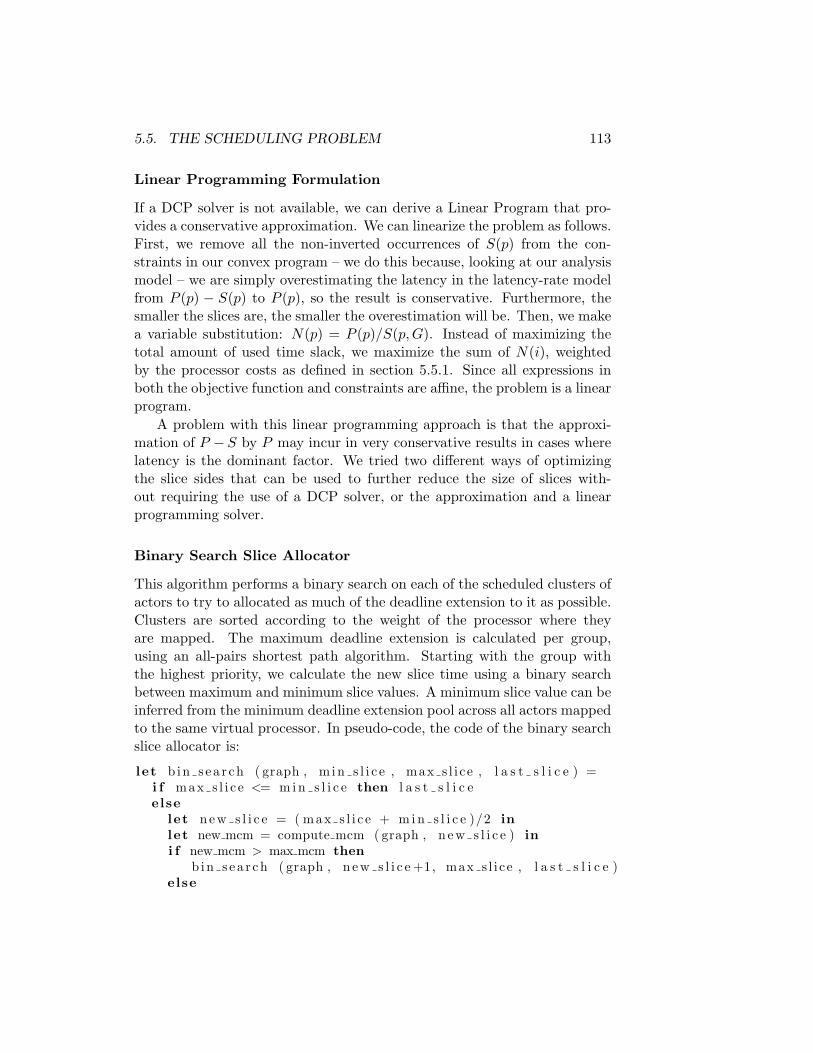
5.5. THE SCHEDULING PROBLEM 113
Linear Programming Formulation
If a DCP solver is not available, we can derive a Linear Program that pro-vides a conservative approximation. We can linearize the problem as follows.First, we remove all the non-inverted occurrences of S(p) from the con-straints in our convex program – we do this because, looking at our analysismodel – we are simply overestimating the latency in the latency-rate modelfrom P (p) − S(p) to P (p), so the result is conservative. Furthermore, thesmaller the slices are, the smaller the overestimation will be. Then, we makea variable substitution: N(p) = P (p)/S(p, G). Instead of maximizing thetotal amount of used time slack, we maximize the sum of N(i), weightedby the processor costs as defined in section 5.5.1. Since all expressions inboth the objective function and constraints are affine, the problem is a linearprogram.
A problem with this linear programming approach is that the approxi-mation of P − S by P may incur in very conservative results in cases wherelatency is the dominant factor. We tried two different ways of optimizingthe slice sides that can be used to further reduce the size of slices with-out requiring the use of a DCP solver, or the approximation and a linearprogramming solver.
Binary Search Slice Allocator
This algorithm performs a binary search on each of the scheduled clusters ofactors to try to allocated as much of the deadline extension to it as possible.Clusters are sorted according to the weight of the processor where theyare mapped. The maximum deadline extension is calculated per group,using an all-pairs shortest path algorithm. Starting with the group withthe highest priority, we calculate the new slice time using a binary searchbetween maximum and minimum slice values. A minimum slice value can beinferred from the minimum deadline extension pool across all actors mappedto the same virtual processor. In pseudo-code, the code of the binary searchslice allocator is:
l et b in s ea r ch ( graph , m in s l i c e , max s l i ce , l a s t s l i c e ) =i f max s l i c e <= min s l i c e then l a s t s l i c eelse
let new s l i c e = ( max s l i c e + m in s l i c e )/2 inlet new mcm = compute mcm ( graph , n ew s l i c e ) ini f new mcm > max mcm then
b in s ea r ch ( graph , n ew s l i c e +1, max s l i ce , l a s t s l i c e )else

114 CHAPTER 5. COMPILE TIME SCHEDULING
b in s ea r ch ( graph , m in s l i c e , new s l i c e −1, n ew s l i c e )
The algorithm can be sped up by not using the MCM computation algo-rithm, but instead relying on using a negative cycle detection algorithm suchas Szymanski [17] to check if the current MCM is still below the maximumMCM allowed (i.e. µD).
The results for this algorithm, however, will depend heavily on whichprocessor and group we start the binary search. The algorithm lowers asmuch as possible the slice time for the first cluster it performs the binarysearch on, sometimes leaving little or no slack that allows the remainingclusters to use to lower their slice times. In fact, its performance is inpractice very similar to the linear program, with the advantage that it doesnot use an approximation for the execution time of the latency actor.
This allocator applies cycle detection at every iteration of a binarysearch. It has polynomial complexity since both cycle detection and binarysearch have polynomial complexity.
Randomized Slice Allocator
We observed that the binary slice allocator depends quite heavily on theclustering ordering on which the search is performed. To overcome thatweakness this algorithm randomly selects clusters to decrease their slicetime by a specific amount, thereby trying to be fair to all clusters. As in theprevious algorithm, if the scheduled graph respects the specified throughputfor some predefined slice times, this algorithm will find smaller or equal slicetimes for the graph thereby decreasing the throughput to as close as possibleto the specified minimum throughput.
The random slice allocator adds all clusters to an open list (i.e. a listof clusters where we may still decrease the slice) and will select a clusterfrom there. The probability of a cluster being chosen for slice decrease isdependent on its weight. That cluster sees its slice time decreased by aspecified amount (pre-defined step of the algorithm) and the graph is testedfor compliance with the throughput constraints. Should the smaller sliceresult in a violation of imposed constraints, that cluster is removed from theopen list and its slice value restored to the previous amount. This select anddecrease step is repeated until there are no clusters in the open list, whichmeans it is not possible anymore to lower slice times while respecting thethroughput constraints.
This algorithm depends also on a cycle detector. Essentially it runs thecycle detector a number of times which depends on the step size and on

5.5. THE SCHEDULING PROBLEM 115
initial cluster’s slice times. The maximum running time for this algorithmcan be bounded and is also a class P algorithm.
5.5.6 Buffer Sizing
Ning and Gao [77] proposed an approach to compute minimal buffer sizesfor an SRDF graph G to allow for rate-optimal execution of the graph, thatis, such that the graph can execute a static-periodic schedule with periodequal to its MCM. Ning and Gao propose a linear program formulation forthis problem which they claimed to be optimal, implying that the prob-lem is solvable in polynomial time, since linear programming is solvable inpolynomial time.
In [72], we have shown that Ning and Gao’s formulation is not optimal,and that the buffer sizing problem is, in fact, NP-complete. Furthermore,we have shown that the constraints of the linear program used by Ning andGao are too conservative: it is relatively simple to derive exact constraints,obtaining a more accurate linear program. In our paper, we have also shownthat, for a randomized input data-set, while the linear program does notyield optimal results, the difference to the optimal solution appears to berelatively negligeable. For a randomized set of connected graphs with 40nodes, only in 50% of the cases did we get overestimation of the buffer sizes,and for these, the average overestimation was 2.1%. The results also seemedto indicate that with the increase of the size of the graphs, the likelihoodof overestimation would increase, while the amount of overestimation woulddecrease.
In our toolset, we implemented our improved version of the buffer sizinglinear program. Other approaches could also be applied, such as the onepresented in [88], which can yield optimal buffer sizes but suffers from ex-ponential complexity, or the approach taken in [92], that applies heuristicsto minimize the buffer size. These approaches were developed at the sametime as the work presented in this thesis. A comparative study of all theproposed solutions still needs to be carried out.
5.5.7 Scheduling Multi-rate graphs
A Multi-Rate Data Flow graph (or, for that matter, a Cyclo-Static DataFlow graph) can be scheduled using our framework, by converting the orig-inal MRDF graph to its equivalent SRDF graph. The conversion does nothave polynomial complexity – the number of copies per actor in the MRDFgraph is given by the number of repetitions in the repetition vector (see

116 CHAPTER 5. COMPILE TIME SCHEDULING
Chapter 3).Care must be taken to ensure that when a SRDF copy a0 of a MRDF
actor a is mapped to a virtual processor p ∈ Π during the static orderingphase, all other SRDF copies ai of the same MRDF node are allocated tothe same processor. The analysis model is also changed to reflect this fact:the values of lat and nat functions for all ai must be computed assumingan allocation to p. If, due to backtracking, the decision to map a0 to p isundone, the allocation of all copies must also be undone.
No changes are necessary to the slicing algorithms.As for buffer sizing, a separate buffer b(ik, jl)can still be calculated for
each arc (ik, jl) ∈ E, where ik is the copy number k of an MRDF actor i, andjl is the copy l of an MRDF actor. Since in the implementation a single bufferis shared to connect all copies of i to j, the static-periodic schedule resultingfrom the buffer sizing linear program is no longer buffer optimal. However, ifwe simulate this static periodic schedule, and count the maximum numberof tokens that are accumulated in every edge during the simulation, weobtain a feasible buffer size for each one of the buffers in the MRDF graph.Govindarajan et al propose another linear-programming approach [32] thatobtains better results by directly deriving buffer constrains from the MRDFgraph. According to the authors, this approach can obtain, in some casesbuffer sizes that are about half of the buffers sizes obtained by the approachwe sketched above. The problem with this approach however, is that thenumber of constraints in the linear program for each edge (i, j) in the isgiven by the product of the repetitions vector entries r(i) and r(j), and thismeans that the linear program can in some cases become too large for thesolver we used in our implementation – the GNU Linear Programming Kit[27] – to handle. Our toolset implements both approaches and leaves to theuser the choice on which to use. Only one of the transceiver graphs we usedin our experiments is a MRDF graph, namely the WLAN receiver presentedin Section 5.6. In this case, the two approaches delivered the same results.
One more remark is needed on buffer sizing. While the work that isbeing reported here was performed, two new approaches have been devisedto solve the buffer sizing problem for MRDF graphs. In [88], an approachis described that provides optimal results. Although the complexity of thealgorithm is exponential, the authors argue that for the extensive set ofrandom graphs that were used to test the approach, the algorithm is inpractice very fast. A heuristic approach has been proposed in [92]. We arenot aware of any extensive comparative study of these approaches.
One possibility that arises from the fact that we can formulate boththe slicing problem and the buffer sizing problems as convex programming

5.5. THE SCHEDULING PROBLEM 117
problems with a conservative linear programming approximation, is thatthe two can be combined onto a single convex programming problem thatsolves the two in tandem. A recently published paper [93] proposes exactlysuch a formulation, although it does not realize that the problem can beexactly solved (for time expressed as a real number) by a convex solver (atleast by CVX), and instead uses an approximation to get rid of the invertedappearances of the slice variables (as we have shown, inversion is a convexfunction for variables that are guaranteed to be positive).
5.5.8 Phase Ordering
It is not trivial to chose in which order to perform the determination of theslice times and the computation of the static order schedule, since these twosteps are strongly interdependent. If one determines the slice times first, thedetermination is based on partial constraints since the schedule is yet to bederived. It may be that there is no valid static order schedule that meetsthe tighter scheduling constraints caused by replacing the original executiontimes by the larger response times due to the chosen time slicing.
An important consideration is that all the algorithms we propose arepolynomial, except for the static order scheduler, which has exponentialcomplexity, and the MRDF to SRDF expansion, if the starting graph is notsingle-rate.
We can determine the static order schedule first, using response timesbased on the maximum allowed slice per processor, S(p), and only afterwardstry to find slice times that are compatible with that static order schedule.Thus, we firts approach the problem as a constraint satisfaction problem, towhich the static order scheduler delivers a feasible solution, if there is one,and then try to optimize this solution by reducing utilization. This has theadvantage that, provided there is a feasible static order schedule, there isalways a solution. However, it may be that the static order schedule chosenis not optimal in the sense that it does not allow for the lowest possibleutilization that meets all the constraints.
A problem with this approach is that the static order scheduler doesnot necessarily produce the solution that allows for the smallest slice sizes.For cases, as in our example, where the execution time of the static orderscheduler permits it, we can run the scheduler inside a loop that searches forlower slice sizes in a way similar to the binary and random slice allocators,with the difference that the whole static order schedule is recomputed insteadof just the MCM, for each attempted combination of slice sizes.

118 CHAPTER 5. COMPILE TIME SCHEDULING
5.6 Example
We will now show how to apply these scheduling techniques to an actual ap-plication in the Software-Defined Radio domain. Assume a multiprocessorsystem designed for baseband decoding. It includes a general-purpose core,an ARM, to handle control and generic functionality, a vector-processorcore, the EVP [8], to handle detection, synchronization and demodulation,and an application-specific Software Codec processor that takes care of thebaseband coding and decoding functions. All these processors are inter-connected via an Æthereal Network-On-Chip [31]. The platform is used tohandle several radio standards (Wireless LAN, TDS-CDMA, UMTS, DVP-H, DRM). In our example we will assume that we want to derive schedulersettings such that we are able to run Wireless LAN (WLAN) 802.11a andTDS-CDMA simultaneously, with independent start and stop, and allow forup to 2 job instances to be active at a time, including configurations withtwo WLAN instances and two TDS-CDMA instances.
Figure 5.8 depicts the timed data-flow model of a WLAN 802.11a job.Execution times (indicated under the actor names) are given in nanosec-onds. The different shading of nodes indicates the different cores to whichthe actors are assigned. Nodes with names starting by “Src” model thesource (inputs from an external RF unit), the nodes “LatencyHeader” and“LatencyPayload” and their adjacent edges are used to convert latency intothroughput constraints, as described in Chapter 4. The source is in thiscase sporadic, but we have seen in Chapter 4 that the maximum latencyassociated with a sporadic source can be bound by the maximum latencyassociated by a strictly periodic source with a rate equal to the minimalinterval between activations of the sporadic source, and therefore we treatthe source as periodic.
For space reasons, the Synchronization step is represented in Multi-RateData flow syntax: 5 “CFESync” nodes process the output of 5 “Src” nodesin a chain of sources and synchronization nodes. The number of “Payload-Demode” actors and respective sources may vary between 1 and 255. Weonly depict the case where there is only one “PayloadDemode” actor. Sourceand Latency actors are not scheduled. This graph has a required maximumproduction period of µD(WLAN) = 40000ns.
Figure 5.9 depicts the timed data-flow graph model of a TDS-CDMA job.The ”Rx” nodes represent the source. The ”Latency” nodes and adjacentedges are used to convert latency into throughput requirements as describedin Chapter 4 (we assume, in this case, a strictly periodic source). Therequired maximum production period is µD(TDSCDMA) = 675000ns.

5.6. EXAMPLE 119
Src1
2400
Src2
800
Detect
220
Hdemode
920
Src3
2400
FFEnCE
680
CFEnSync
355
Src4
1600
Src5
2400
Src7
4000
Src6
4000
HDecode
920
PDemode
920
PDecode
920
MacCRC
500
MacAnalyse
1000
BuildHeader
500r
CodeHeader
920
LatencyHeader
20000
AckCodeAckMode
920
LatencyPayload
20000
SIFS
16000
ModHeader
920
5:1
5:1
1:5
1:5
Figure 5.8: A Wireless LAN 802.11a receiver job.
Src1
275000
Src2
12500
DASS
19000
JD1
27500
Src3
100000
MI
42000
CE
33000
Src4
287500
DecCRC1
25000
JD2
15500
DecCRC2
25000
TFCI
2000
TPC
1000
Latency2
285500
Latency3
395000
Latency1
285680
Figure 5.9: A TDS-CDMA job.

120 CHAPTER 5. COMPILE TIME SCHEDULING
Weights Utilization (%)EVP SwC ARM EVP SwC ARM
1 1 1 45 45 212 1 1 28 45 452 2 1 28 45 451 2 1 45 28 45
Table 5.2: WLAN scheduling results.
We start by choosing time wheel periods. We assume a worst-casecontext-switch time of 100ns for all processors. We want to support twojobs at a time and we would like to spend less than 10% of our time context-switching, so we set our wheel time to 2000ns. Therefore, P(EVP)=2000,P(SWC)=2000, P(ARM)=2000.
As we want to be able to run two WLAN or two TDS-CDMA jobs si-multaneously, we set the maximum utilization per processor at 45%, (halfprocessor utilization minus context-switching overhead). That is, the maxi-mum slice size for any processor is S(p) = 0.45× P (p).
For both jobs, we first computed static order schedules and then timeslice extensions. In both cases, a static order schedule that meets the timingconstraints (including the S(p) limitation on slice size per processor) wasfound. These schedules were used to calculate slice time optimizations. Wevaried the values of the costs of the three processors to search for trade-offs.It turns out that the algorithms tends heavily towards allocating all slackto a particular processor. A change in weights typically forces a drasticchange from allocating slack to one processor to another, making this ap-proach essentially equivalent to a binary search with weights associated withprocessor types.
In the case of the WLAN – the results are shown in Table 5.2 – varyingthe weights for each processor type allowed us to decrease the utilization ofone of the processors from 45% to 28%. The table pretty much exhauststhe possible trade-offs. It suggests that it makes sense to keep a table withseveral configurations and allow the admission controller to chose differentTDM settings for a job instance taking into account the current level ofresource utilization.
The results for the TDS-CDMA are shown in Table 5.3. One thing tonotice here is that the optimal slice times for the ARM and the SoftwareCodec are obtained for equal weights. Increasing the weights of either ARMor Software Codec by any amount didn’t further decrease their slice times.
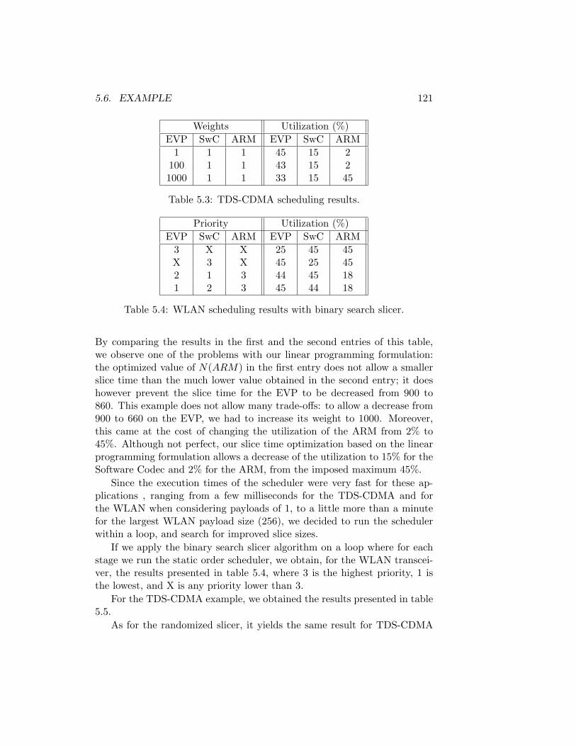
5.6. EXAMPLE 121
Weights Utilization (%)EVP SwC ARM EVP SwC ARM
1 1 1 45 15 2100 1 1 43 15 21000 1 1 33 15 45
Table 5.3: TDS-CDMA scheduling results.
Priority Utilization (%)EVP SwC ARM EVP SwC ARM
3 X X 25 45 45X 3 X 45 25 452 1 3 44 45 181 2 3 45 44 18
Table 5.4: WLAN scheduling results with binary search slicer.
By comparing the results in the first and the second entries of this table,we observe one of the problems with our linear programming formulation:the optimized value of N(ARM) in the first entry does not allow a smallerslice time than the much lower value obtained in the second entry; it doeshowever prevent the slice time for the EVP to be decreased from 900 to860. This example does not allow many trade-offs: to allow a decrease from900 to 660 on the EVP, we had to increase its weight to 1000. Moreover,this came at the cost of changing the utilization of the ARM from 2% to45%. Although not perfect, our slice time optimization based on the linearprogramming formulation allows a decrease of the utilization to 15% for theSoftware Codec and 2% for the ARM, from the imposed maximum 45%.
Since the execution times of the scheduler were very fast for these ap-plications , ranging from a few milliseconds for the TDS-CDMA and forthe WLAN when considering payloads of 1, to a little more than a minutefor the largest WLAN payload size (256), we decided to run the schedulerwithin a loop, and search for improved slice sizes.
If we apply the binary search slicer algorithm on a loop where for eachstage we run the static order scheduler, we obtain, for the WLAN transcei-ver, the results presented in table 5.4, where 3 is the highest priority, 1 isthe lowest, and X is any priority lower than 3.
For the TDS-CDMA example, we obtained the results presented in table5.5.
As for the randomized slicer, it yields the same result for TDS-CDMA

122 CHAPTER 5. COMPILE TIME SCHEDULING
Priority Utilization (%)EVP SwC ARM EVP SwC ARM
X X X 21 8 1
Table 5.5: TDS-CDMA scheduling results with randomized search slicer.
Priority Utilization (%)EVP SwC ARM EVP SwC ARM
1 1 1 33 36 36
Table 5.6: WLAN scheduling results with binary search slicer.
as the binary slicer since, for this transceiver, the minimum slice values foreach processor are seemingly independent of the others. This has to do withthe fact that the cycle that becomes the most critical when we reduce theresource allocation for each of the processors is different. For the EVP, thisis a cycle that includes the edge between Latency2 and Source1. For theSoftware Codec, it is the cycle between DecodeCRC1 and DecodeCRC2. Asfor the ARM, we obtained in both cases the lowest utilization we considered(1%).
In the WLAN case, the randomized slicer yields other slice allocationsdepending on the weights given to the processor types. By giving the sameweights to the 3 processor types, and using a step equal to 1% of the period,we obtained a slice distribution such as the one shown in table 5.6.
As for the buffer sizing, we ran the buffer sizing algorithm before andafter static ordering and slicing, and obtained exactly the same results.This may be accounted for by the relatively few possibilities for pipelinedexecution within the graphs of these applications. Most radio applicationswe studied (UMTS, LTE, DVB-T, DVB-H), however, seem to have relativelysimilar structures.
The best choice for ordering the stages in the scheduler may be verydependent on the characteristics of the specific application and platform. Inthis case, the relatively small execution times of the static order schedulerallowed us to run a full search for schedules to optimize the slice sizes.The relatively small search space for optimal buffer allocation made mootthe choice of when to perform buffer sizing. This may vary widely fromapplication to application, requiring flexibility in the implementation of thescheduler. Since the temporal impact of all the decisions can be simplymodeled in a data flow graph, all scheduling decisions can be imposed aspre-conditions to any stage of the scheduler, making it simple and easy to

5.7. RELATED WORK 123
re-order the stages of the scheduler, or even merging them.
5.7 Related Work
Much work has been published on the scheduling of data flow graphs withreal-time requirements. The level of dynamicity we allow in the start andstop of jobs is what basically differentiates our problem from other multipro-cessor real-time scheduling problems. We will review proposed approachesthat could be adapted to solve our problem.
The most viable alternative to our solution is to use pre-compiled re-source allocation configurations, such as in CPA [85]. For each job-mix, aseparate optimal static schedule is derived at compile time and stored ina look-up table. During operation, when there is a request to start a job,the runtime system checks which jobs are active and selects the appropriateconfiguration. This approach is not without problems. First, a differentconfiguration has to be stored for each combination of jobs, which meansthat the number of configurations grows exponentially with the number ofjobs. Second, if a job is not known at design time, it will force a wholenew set of configurations to be compiled later. Third, it is difficult to as-sure continuity of execution of already running jobs during reconfiguration.For continuity, a configuration should be generated for each transition froma job-mix to another which easily becomes infeasible because of the largeamount of configurations that may need to be generated.
We calculate scheduling budgets per job at compile time. During runtimetwo distinct temporal phases alternate: configuration phase and steady-stateexecution phase. During configuration phases, resources are allocated tojobs; during steady-state resource allocation is fixed. In this, our strategycan be compared with semi-static techniques [16], where system executionis divided in phases and resource allocation is redone at the beginning ofeach phase. But while in semi-static systems phases are periodical, in ourcase reconfiguration phases are triggered by an external request to start orstop a job. Also, in our approach, an actor, once placed cannot be movedto another processor.
Our strategy has similarities with other time-multiplexing strategies suchas gang scheduling [19]. Our jobs correspond roughly to a ’gang’, i.e. a groupof tasks (actors in our case) with data dependencies. There is, however,an important difference: in gang scheduling, time-multiplexing is global,i.e., the temporal slots are uniform across all processors, and synchronizedcontext-switching is required. In our case, time-multiplexing is local to

124 CHAPTER 5. COMPILE TIME SCHEDULING
each individual processing element. Our strategy has several advantagesover gang scheduling: it does not require global synchronization of contextswitches, which hinders design scalability; it leaves less unused resourcesbecause its time sharing is more fine grained; and it also allows for a differentscheduling mechanism per processor.
Stuijk[88] describes a method with many similarities to ours, since italso mixes static order and TDM scheduling for homogeneous multiprocessorsystems. It does not consider non-preemptive scheduling or heterogeneoussystems. It does not address different start/stop times. To account for theeffect of TDM on the response times, simulation of the self-timed executionof the data flow graph with worst-case response times is performed, whilekeeping track of the state of the TDM wheels. For this to yield conservativeresponse times, all possible states for a worst-case, self-timed schedule shouldbe simulated, which seems to imply that conservative results require thatsimulation continues until the same token positions and the same positionon all TDM arbiters is reached simultaneously, which can lead to an expo-nential blow-up. This work also differs from ours in that actor to processormapping and static ordering are decoupled. First an heuristic is appliedto find a processor mapping, and then static order schedule is determinedby a ready-list scheduler with no backtracking and no timing constraints,which means that the static order schedule has one single chance at findinga feasible order. No explicit heuristic is proposed to decide which of two si-multaneously ready actors mapped to the same processor is scheduled first.If the static order scheduler fails, the tool simply does a new mapping andtries again to statically order it. Slice minimization is done using binarysearch after static ordering, using data flow simulation to check for timingconstraint violation at each step. In this approach, only TDM schedulerscan be supported as timing analysis is dependent on the simulation of theTDM time-wheels.
5.8 Conclusion
In this chapter we present a scheduling strategy and a scheduling flow tosolve the problem of running multiple jobs with different rates and differentstart/stop times on a heterogeneous multiprocessor. The scheduling strat-egy involves a combination of static order scheduling per job per processor,and TDM or Non-preemptive Non-blocking Round Robin scheduling to ar-bitrate between different jobs in each processor. We have shown how thecombination of dynamic scheduling with static order scheduling is desirable

5.8. CONCLUSION 125
and can be modeled for the purpose of temporal analysis. We have shownhow the temporal analysis model can serve as a basis for a scheduling flow.We have proposed algorithms to estimate the temporal slack that can beallowed per actor for a timed SRDF, and how to exploit this time slack bydecreasing slice times. This flow solves a practical problem arising in real-time streaming platforms (Software-Defined Radio, Car Radio, Digital TV)and is unique in that it is able to find both TDM settings and static orderschedules per job per processor, to handle a dynamic job-mix on a multipleprocessor and provide hard real-time guarantees for all admitted jobs.
Although we present our flow using Time-Division Multiplex and Non-Preemptive Non-Blocking Round Robin for inter-job scheduling, this doesnot present an essential limitation of the techniques: any scheduler that canbe represented by a latency-rate model can be used, although changes mayneed to be made to the computation of scheduler settings. Also, any newdata flow model of a scheduler can be easily supported by simply changingmodel generation to create different actors and edges.
There are several open issues we wish to address in future work. One isproposing a heuristic approach to perform the clustering and static orderingof actors, since the current algorithm is exponential and, although it is man-ageable in the relatively small graphs of the transceivers we studied, it doesnot scale easily to larger graphs (and larger graphs can arise from MRDFto SRDF conversion for even relatively small MRDF graphs). Furthermore,the current approach allows communication and buffer capacity constraintsto be taken into account, but it is also interesting to search for schedulingsettings that optimize for low communication requirements and/or smallbuffer sizes.

126 CHAPTER 5. COMPILE TIME SCHEDULING

Chapter 6
Mode-Controlled Data Flow
In the process of choosing a Data Flow (DF) programming model for de-scribing an application, one must make a difficult trade off between expres-siveness and analytical properties. At one extreme, a Dynamic Data-flow(DDF) model is expressive enough to mimic the behavior of a Turing ma-chine [10], but lacks many useful analytical properties; for instance, for anarbitrary DDF graph it may be impossible to verify if it is free of dead-locks, or if it can execute for indefinite time on bounded buffer space [10].On the other hand, Static Data flow (StDF) variants (such as SynchronousDF [58], Homogeneous Synchronous DF [81], or Cyclo-Static DF [9]) allowfor powerful analysis, such as the verification of deadlock-freedom, determi-nation of maximum achievable throughput, and verification of latency andthroughput constraints, but have limited expressivity: they can only expressapplications that work with fixed data rates, i.e., all quantities of data sen-t/received per actor firing cannot be dependent on the values of the inputdata. Because of these limitations, StDF models tend to be reserved for ap-plication domains where task activation is data-driven, data rates regular,and real-time guarantees required.
For the most, this is the case for Base-Band Software-Defined Radio(SDR) [8]. On a typical digital baseband algorithm, data flows through threeprocessing stages: filtering, modulation/demodulation and coding/encod-ing. Broadcast standards typically have throughput requirements that mustbe met, while bi-directional communication standards also impose maximumlatencies.
StDF computation models have already been proposed [62] for usage inthis domain. One problem with such an approach is that some SDR appli-cations are subject to occasional changes of operation mode, i.e. changes in
127

128 CHAPTER 6. MODE-CONTROLLED DATA FLOW
the sequence of algorithms that must be executed to process the incomingstream. A DVB-H receiver, for instance, executes the same demodulation-decoding flow of streaming tasks during most of its operation, but duringinitiation and occasionally during its active state it needs to execute a differ-ent sequence of tasks in order to achieve synchronization with the incomingstream. This synchronization mode takes an unknown number of iterationsto succeed. Therefore, while static data rates can be used to represent themessage passing within each synchronization attempt, the same cannot bedone to represent the dependencies and data communication between syn-chronization and decoding modes.
A more severe problem can be observed in another SDR application:Wireless LAN (WLAN). On a WLAN 11a receiver, packet detection is per-formed in a loop in the RF interface until it succeeds. Then, the basebandstarts executing. First, synchronization is performed. If this is success-ful, a demode-decode sequence will be executed for each received symbol,until the variable-sized payload of the packet is fully processed. Each ofthese operation modes can be expressed as an (analyzable) StDF graph.The change from mode to mode, however, cannot be expressed within theconfines of StDF. In terms of DF, a change of operation mode is more likea change of the computation graph. However, for SDR applications, hardreal-time requirements may be defined across operation mode transitionsand therefore temporal analysis is only useful if mode transitions can betaken into account. Such is the case with the WLAN 11a example, wherethere is a maximum allowed latency from the time when the packet startsto be sent and the moment when the receiver sends an acknowledgment ofpacket reception to the sender. To make the problem more complex, thereare data dependencies between modes, such that the execution of each modeis conditioned by the schedule of the previous one.
The behavior during one of these mode transitions cannot be conve-niently expressed in StDF. One solution that we have used in the past is foran analysis specialist to design an StDF model that represents worst-caseassumptions about the execution of a given, concurrent WLAN receiverimplementation that does not necessarily conform to the strict StDF con-struction rules. The StDF model can then be used for temporal analysis andscheduling purposes. One such model was used for our WLAN 11a examplein Chapter 5.
This approach is slow, difficult, and requires both data-flow modelingexpertise and in-depth knowledge of the application. Furthermore, it isimpossible to guarantee that the model does indeed conform to the actualimplementation. What we would like to have is a programming model that

6.1. MODEL OVERVIEW 129
enables the automatic extraction of an analysis model. However, for thatthe programming model has to be powerful enough to describe these modetransitions and still allow for hard-real-time analysis.
In this chapter we propose a DF programming model that can be seen asa restriction of Boolean DF that allows for mode switching without compro-mising the properties that make the graph amenable to temporal analysis,and keeping the programming model as simple as possible. For need of aname, we refer to this restricted model as Mode-Controlled DF (MCDF).The chapter is organized as follows: in the next section, we present anoverview of our data flow model; in the following section, we describe in de-tail the new types of data flow actors we introduce; in Section 6.3 we presentthe rules to construct a well-constructed MCDF graph; Section 6.4 showshow radios can be modeled in MCDF, by providing two examples, a DVB-Treceiver and a WLAN 802.11a receiver; Section 6.5 discusses the basic an-alytical properties of well-constructed MCDF graphs; Section 6.6 providestechniques for temporal analysis of MCDF graphs; Section 6.7 describes thescheduling techniques we developed for MCDF graphs; Section 6.8 describesthe results we obtained from scheduling a WLAN receiver modeled as anMCDF graph on a multiprocessor platform; Section 6.9 discusses relatedwork; and Section 6.10 concludes the chapter.
6.1 Model Overview
Intuitively, a Mode-Controlled DF graph is a data flow graph where foreach firing of a designated actor, called the Mode Controller (MC), actorsbelonging to a specific, pre-defined subgraph of the complete MCDF graphare fired. A specific subgraph is chosen for firing, depending on an outputvalue produced by the Mode Controller. Therefore there are data-dependentactor firings. After all actors in the chosen subgraph have fired, the graphreturns to the initial token distribution. An iteration of an MCDF graphcorresponds to the firing of all actors in one of these subgraphs. The modelallows verification that no deadlocks can occur and behavior is kept deter-ministic in the Kahn Process Network [49] sense, i.e., provided that FIFOcommunication is blocking, and that the internal functionality of actors hasno notion of time, the outcome of the computations is independent of thetime at which the actors are activated.

130 CHAPTER 6. MODE-CONTROLLED DATA FLOW
6.2 MCDF Constructs
In this section we will describe the main building blocks of a Mode-ControlledDF graph.
6.2.1 The Mode Controller
The Mode Controller (MC) is a special node in MCDF. The special charac-teristic of the MC is that one of its outputs drives the control input portsof all data-dependent actors in the MCDF graph. We refer to this specialoutput port as the mode control port. At each firing, the MC producesa single token in the mode control port, and there are no delays on theedges that connect the mode control port to the control input ports of alldata-dependent actors.
For any given MCDF graph, there is a fixed number of modes, M . Thevalue of the token produced by the MC in the Mode Control port has tobe an integer within the closed interval from 1 to M . This value representsthe mode selected for the current iteration of the MCDF graph. Tokensproduced through the mode control port are referred to as control tokens.
6.2.2 Data-dependent Actors
Besides SRDF actors, an MCDF graph allows the usage of three types ofdata-dependent actors. These are the Mode Switch, Mode Select and ModeTunnel actors. However, as we shall see, the Mode Tunnel, can be repre-sented by using both a Mode Switch and a Mode Select actors, and shouldbe regarded as a convenient short-hand notation that we offer to the pro-grammer to allow inter-mode communication.
The data-dependent actors have in common the fact that they all have acontrol input port. A control token is read from this port for each firing ofthe data-dependent actor. That value determines which other ports of theactor are producing/consuming data during this firing. Control tokens areproduced and consumed as normal tokens.
Definition 6.1. A port is said to be associated with mode m if the con-sumption of a token with value m on the control input port causes data to beproduced/consumed on this port, while the consumption of any other valuewill not cause data to be produced/consumed on this port.
Definition 6.2. A Mode Switch actor (Figure 6.1(a)) has, besides thecontrol input port, one data input port and M output ports. Each output

6.2. MCDF CONSTRUCTS 131
port is associated with a mode. When a token is present on the control inputport and on the data input port, the Mode Switch actor is fired. It consumesboth input tokens and produces a token in the output port associated with theMode indicated by the token consumed on the control input port. The outputtoken has the same size and value as the token consumed on the data inputport.
Definition 6.3. A Mode Select actor (Figure 6.1(b)) has, besides thecontrol input port, M data input ports and one output port. Each input portis associated with a mode. When a token is present on the control inputport, its value is read and used to decide from which input port to consumea token. The actor is fired when a token is present in the control input portand in the data input port associated with the mode indicated by the tokenin the control input port. When fired, it consumes both of these tokens. Atthe end of the firing, it produces on the output port a token with the samesize and value as read from the modal input port. If the input port was notconnected, the output token will have some pre-defined default value, whichcan be mode dependent. Note that, as in the BDF Select, the firing rule mustbe evaluated in two steps.
Besides these two canonical types of data-dependent actors, we introducea third type, the Mode Tunnel. Mode tunnels are in fact a shorthand for aconstruct involving both a Mode Switch and a Mode Select actor, and forthat reason, they will be absent on our study of the properties of MCDFgraphs. They are, however a very useful construct for programmers, as theyallow the communication between different modes.
Definition 6.4. A Mode Tunnel actor (Figure 6.1(c)) has, besides thecontrol input port, one data input port and one data output port. The datainput port is associated with an arbitrary mode m of the graph, and thedata output port is associated with a mode n of the graph, different from m.When the token read at the control input port has the value m, the ModeTunnel fires and consumes a token from the control input port and fromthe data input port. It stores the token read from the data input port in itsinternal state. When the control input port has value n, the Mode Tunnelfires, consuming that value and copying the token stored in its internal stateto the data output port. The initial value of the internal state is graph-specific. In this way, the Mode Tunnel always delivers to its consumer thevalue produced by the last previous execution of the source orchestrated bythe Mode Controller. As with Select and Mode Select, the firing rule of ModeTunnel must be evaluated in two steps. We refer to a Mode Tunnel as an
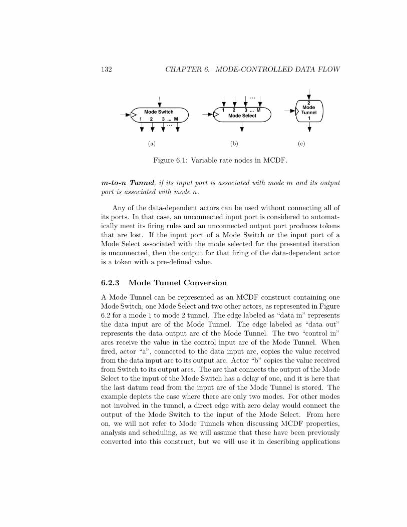
132 CHAPTER 6. MODE-CONTROLLED DATA FLOW
Mode Switch 1 2 3 ... M
...
(a)
1 2 3 ... M Mode Select
...
(b)
2ModeTunnel
1
(c)
Figure 6.1: Variable rate nodes in MCDF.
m-to-n Tunnel, if its input port is associated with mode m and its outputport is associated with mode n.
Any of the data-dependent actors can be used without connecting all ofits ports. In that case, an unconnected input port is considered to automat-ically meet its firing rules and an unconnected output port produces tokensthat are lost. If the input port of a Mode Switch or the input port of aMode Select associated with the mode selected for the presented iterationis unconnected, then the output for that firing of the data-dependent actoris a token with a pre-defined value.
6.2.3 Mode Tunnel Conversion
A Mode Tunnel can be represented as an MCDF construct containing oneMode Switch, one Mode Select and two other actors, as represented in Figure6.2 for a mode 1 to mode 2 tunnel. The edge labeled as “data in” representsthe data input arc of the Mode Tunnel. The edge labeled as “data out”represents the data output arc of the Mode Tunnel. The two “control in”arcs receive the value in the control input arc of the Mode Tunnel. Whenfired, actor “a”, connected to the data input arc, copies the value receivedfrom the data input arc to its output arc. Actor “b” copies the value receivedfrom Switch to its output arcs. The arc that connects the output of the ModeSelect to the input of the Mode Switch has a delay of one, and it is here thatthe last datum read from the input arc of the Mode Tunnel is stored. Theexample depicts the case where there are only two modes. For other modesnot involved in the tunnel, a direct edge with zero delay would connect theoutput of the Mode Switch to the input of the Mode Select. From hereon, we will not refer to Mode Tunnels when discussing MCDF properties,analysis and scheduling, as we will assume that these have been previouslyconverted into this construct, but we will use it in describing applications

6.3. MCDF CONSTRUCTION RULES 133
modeled as MCDF, as it greatly simplifies models where values must becommunicated between modal actors from different modes.
Switch 1 2
ba
1 2Select
data in data out
control in
control in
Figure 6.2: Construct to represent Mode Tunnel in terms of Mode Switch,Mode Select and SRDF actors.
6.3 MCDF Construction Rules
The rules we will present for the construction of a well-constructed MCDFgraph are designed to guarantee that it can always return to the initial stateof token placements independently of the sequence of mode control tokensgenerated by the Mode Controller. More specifically, we want to ensurethat each firing of the MC enables all actors pertaining to a mode and allactors not specifically pertaining to any mode to fire until all edges returnto the initial state, without any other activation of the Mode Controllerbeing required. Here we will assume that all actors that do not have data-dependent behavior are single-rate. In Section 6.9 we will discuss how themodel can be extended to multi-rate actors.
An MCDF graph with M modes is composed of:
• A Mode Control actor (MC);
• an arbitrary number of Mode Select, Mode Switch actors;
• an arbitrary number of static, single-rate actors
Now, we will define some terminology which will help us specify the con-struction rules.
Definition 6.5. Two ports are said to be connected if and only if thereis an arc between them in the graph. In the same way, two actors are said

134 CHAPTER 6. MODE-CONTROLLED DATA FLOW
to be connected if and only if there is an input port of one of them and anoutput port of the other that are connected.
Definition 6.6. An edge is said to be delay-less if its delay valuation iszero. A path is said to be delay-less if all the edges that it traverses aredelay-less.
Definition 6.7. Actor Modality Actors in an MCDF graph are annotatedwith a valuation mode: V → 1, ...M. Since only some actors execute forspecific modes, mode is a partial function. If mode(i) is defined, then theactor is said to be modal and we can say that actor i belongs to mode(i).If mode(i) is undefined, denoted by mode(i)= ⊥, the actor is said to beamodal.
Please note that modal actors do not have a mode control port. The onlyactors to have a mode control port are the data dependent actors, ModeSwitch and Mode Select (and Mode Tunnel), which are always amodal, i.e.are fired in all iterations, independent of the value of the mode control token.The Mode Controller itself amodal, and its firing condition is data-valueindependent.
Definition 6.8. Actor Type There are some actors in MCDF that havespecial attributes, these are the Mode Controller, the Mode Switch and theMode Select. We use valuation atype: V → mc, switch, select, normal, toindicate any special attributes of an actor.
An MCDF graph is defined by the tuple G = (V,E, t, d,M,mode, atype),where V is the set of actors, E is the set of edges, t is the timing valuation ofactors, d is the integer-value delay of edges, and M is the number of modesin the graph, mode is the mode valuation of actors and atype is the actortype valuation for actors.
Definition 6.9. The Mode m Subgraph of G is a sub-graph Gm =(Vm, Em, t, d) of MCDF graph G = (V,E, t, d,M,mode, atype), such thatits vertex set Vm is composed of all amodal actors, and all actors that belongto mode m, and its edge set is composed of all edges which are in E andwhose sources and sinks both belong to Vm, and where t and d are restrictedto Vm .
To simplify the notation, we will not explicitly model ports. We followa number of assumptions about ports: if a modal node is connected to adata-dependent actor such as a Mode Switch or Mode Select, it is alwaysto a port associated with its mode. Furthermore, an output port can be

6.3. MCDF CONSTRUCTION RULES 135
connected to multiple edges – i.e. the value produced through that port isproduced onto all edges connected to it – such a port can be referred to as amulti-port. The mode control port is a multi-port if there are more than onedata-dependent actors (i.e. Mode Switches and Mode Selects). An inputport can only be connected to a single edge.
The construction rules that must be respected by a MCDF graph for itto be considered well-constructed are as follows:
Rule 1. There is only one mode controller.
Rule 2. Modal actors can either be connected to other modal actors, assinks to the output ports associated with their mode on Mode Switches, oras sources to the input ports associated with their mode on Mode Selects.On the other hand, the ports of amodal actors other than the output ports ofMode Switches and the input ports of Mode Selects, can only be connected tofixed rate ports of other amodal actors. This means that, if G is an MCDFgraph, for edge (i, j) ∈ E it must hold that
(mode(i) = mode(j)) ∨ (atype(i) = switch ∧mode(j) 6= ⊥)∨(atype(j) = select ∧mode(i) 6= ⊥)
Rule 3. The mode control output port of the Mode Controller is connectedto all control input ports in the graph through delay-less edges. This meansthat for any edge (i, j) ∈ V where atype(i) = mc it must hold that
d(i, j) = 0 ∧ (atype(j) = switch ∨ atype(j) = select) (6.1)
Rule 4. There are no delay-less cycles in the graph.
Rule 3 ensures that there is a single condition that drives all data-dependent actors. Furthermore, it guarantees that for the same firing countthe same mode control token is read by all data-dependent actors, i.e. if thenth firing of a given data-dependent actor activates its ports associated withmode m, then we can expect the nth firing of another data-dependent actorin the graph to activate its own ports associated with mode m.
The concept of iteration for MCDF is the same as for SRDF: a sequenceof actor firings that brings the graph back to the initial token distribution.The difference is that in MCDF not all actors fire on each iteration. In fact,as we shall prove, only amodal actors fire once per each iteration, and thecount of completed iterations of the graph is equal to the number of firingsof MC.
Rule 4 is needed to obtain deadlock-free graphs. A cycle with no delayswould create a cyclic dependency between firings on the same iteration whichwould eventually deadlock the execution of the graph.

136 CHAPTER 6. MODE-CONTROLLED DATA FLOW
6.4 Radio Modeling in MCDF
MCDF was designed to allow the easy expression of modal behavior in trans-ceivers. In this section, we will provide two examples of how radios can bemodeled in MCDF: a DVB-T receiver and a Wireless LAN 11a receiver.
6.4.1 Example Application: DVB-T receiver
Figure 6.3 depicts our MCDF model for a DVB-T receiver application. TheDVB-T receiver requires an MCDF graph with 3 modes: mode 1 handlessynchronization, mode 2 simply drops input data and mode 3 demodulatesand decodes the input data and sends it to the output stream. Both in syn-chronization and demodulation modes, the DVB-T receiver must regulatethe timing and frequency of the receiver analog front-end. This is repre-sented by an analog control that is issued by the “sync” actor in mode 1and by the “dem” actor in mode 3, that is sent through a mode select backto the source. As for the operation of the mode controller, it selects, in thefirst iteration, the synchronization mode. It will continue to operate in thismode until synchronization with the incoming stream is detected. In thatcase, the receiver must align itself with the beginning of a DVB-T frame,and, for a number of rounds determined by the outcome of synchronization,it will drop input data. It will then go into demodulation mode (mode 3),where it will stay until either the receiver is stopped or synchronization islost, in which case it will go back to the synchronization mode. The require-ment for this receiver is that no matter what mode it is running, it keepsup with the period of the source (about 900 µs).
6.4.2 Example Application: Wireless LAN receiver
Figure 6.4 depicts the timing of a WLAN 802.11a packet. In a WLAN802.11a receiver, baseband processing starts once a packet is detected atthe RF. First, synchronization is performed over the first 8µs. These aretwo groups of 5 short symbols – 5 short symbols are equivalent to one longsymbol. If this is successful, the packet header is demodulated and decodedto determine the size of the payload. After this, the OFDM symbols of thevariable-sized payload – from 1 to 256 OFDM symbols, each with a lengthof 4µs – are processed one by one by a demode-decode loop, followed by aCyclic-Redundancy Check (CRC). If CRC is successful, an acknowledgmentpacket must be sent within 16µs of the end of reception. This time guardof 16µs is known as the Short Intra-Frame Spacing (SIFS).

6.4. RADIO MODELING IN MCDF 137
switch 1 2 3 mc
drop
sync
1 2 3 select1
source
dem dec
sink
1 2 3select2
acq
Figure 6.3: MCDF graph for a DVB-T receiver.
Preamble PayloadHeader
OFDMShort Symbols Long Symbols
OFDM OFDMHeader
IEEE 802.11a WLAN packet
LLS SSS SS SS S
10x 0.8 µs 2x 4.0 µs
S
4.0 µs 4.0 µs 4.0 µs 4.0 µs
Figure 6.4: WLAN 802.11a packet structure.
138 CHAPTER 6. MODE-CONTROLLED DATA FLOW
Figure 6.5 depicts our MCDF model for a Wireless LAN receiver ap-plication. Arcs that communicate control tokens are depicted by dashedlines. The graph has 4 modes: Synchronization (mode 1), Header Process-ing (mode 2), Payload Processing (mode 3) and CRC (mode 4). The inputfrom the RF source (“source” actor) is sent to the “shift” actor, which per-forms alignment at the start of each OFDM symbol, by pre-pending theend of the previous token to the current one, and storing the remainder ofthe current token to pre-pend to the next. The length of the prefix is firstset to 0, and is later determined during synchronization, and transmittedto “shift” through the Mode Controller, that received it from the Mode Se-lect “select” actor. From “shift’,’ data is sent through the Mode Switch“switch” to the mode selected by “mc.” The decoding of a packet startswith “mc” selecting mode 1. At the end of each firing, “sync” informs “mc”through “select” whether it succeeded to synchronize. Depending on theoutcome, “mc” will choose whether to fire mode 1 again, or start process-ing the header. Also,“mc” sends to “shift” the current value of the offset,as given by the return value of mode 1, received from “select”. Mode 2fires two modal actors: one on the EVP (“hdem”) and the other on thesoftware codec (“hdec”). The status sent by “hdec” to “mc” via “select”indicates the length of the payload. Also, through a Tunnel from mode 2 to3, several demodulation parameters for this message are communicated tothe “pdem” actor that does the demodulation of payload symbols in mode3. For a number of firings equal to the length of the payload, “mc” willselect mode 3, firing actor pdem in the EVP followed by actor “pdec” in theSoftware Codec. Once the full payload has been received, “mc” will selectmode 4 for execution, activating the consumer side of the Tunnel betweenactors “pdec” and “crc”. The “crc” actor executes in the ARM processor.After the CRC check is completed, a response message is encoded in theSoftware Codec (actor “code ack”), modulated in the EVP (actor “modeack”), and sent to the base-station through the RF. Notice that only whenmodes 1 or 2 are selected is the decision of the Mode Controller dependenton the last input data. For modes 3 and 4, decisions can be taken aheadof this, and in the graph this is reflected by the fact that “select” can im-mediately generate a data token to fire again “mc” without waiting for anyof the modal actors. Notice also that for the execution where “mc” selectsmode 4, data from the source is discarded, since the output port of “switch”for mode 4 is not connected.
In the next iteration, “mc” reverts to its initial state and the graph isready to process a new incoming packet.

6.5. PROPERTIES 139
switch 1 2 3 mc
hdem
sync
1 2select
hdec
pdec
source
dataout
pdem
crc
codeack
modeack
sendheader
sendpayload
shift
2:3 Tunnel 3:4
Tunnel
Figure 6.5: MCDF graph for a WLAN 11a receiver.
6.5 Properties
In this section we will discuss relevant analytical properties of MCDF graphs.Some important temporal properties of Mode-Controlled Data-Flow stem
from two facts: 1) MCDF is a subset of Integer-Controlled DF (IDF) ([10] –see Chapter 3), and therefore inherits all its properties; 2) a tight worst-casetiming model of its execution can be built that conforms to the SRDF modeland allows us to transpose some SRDF properties to MCDF graphs.
Other properties stem from the choice we made on defining the con-struction rules. In the following sections, we will present some importantproperties of MCDF, and provide proofs that they hold.
6.5.1 Notation
Consider an MCDF graph G = (V,E, t, d,M,mode, atype), where V is theset of actors, E is the set of edges, t is the timing valuation of actors, d is theinteger-value delay of an edge, and M is the number of modes in the graph,mode is the mode valuation of actors and atype is the actor type valuationfor actors.
140 CHAPTER 6. MODE-CONTROLLED DATA FLOW
Let a sequence c = [m1,m2, ...,mn], with mk ∈ 1, ...,M represent themode control sequence, i.e., the sequence of values of the tokens producedby the mode controller on a given execution of the MCDF graph. Let c(k)return the value of the tokens produced by the mc node on its (k + 1)th
firing, or the kth element of c.
6.5.2 Determinism
Any MCDF graph is also an IDF graph, and has all the properties of IDFgraphs. Therefore, it is deterministic, in the same sense as Kahn’s ProcessNetworks [49]: given the same input history (i.e given a specific sequence ofvalues produced by the firings of the source actor), an MCDF graph alwaysproduces the same exact output, independently of the time at which eachactor firing happens.
6.5.3 Linear Timing
Another interesting property of MCDF is the linear timing of its sched-ules. We proved that this property holds for self-timed schedules of SRDFgraphs in Chapter 4. Take a self-timed schedule s(i, k) of a data-flow graphG = (V,N, t, d) . Then, if the (n+1)th firing of a given actor a ∈ N is delayedby a time interval of ∆ such that its new firing time is s′(a, n) = s(a, n)+∆,then s′ is guaranteed to be an admissible schedule of the graph if, for allfirings dependent on firing (a, n), s′(i, j) = s(i, j) + ∆, while for firings in-dependent of (a, n), s(i, k) = s′(i, k) . Note that in SRDF an actor firing(i, k) is dependent on (a, n) if, by recursively applying 4.2 we find an ex-pression dependent on s(a, n). This theorem holds because the firing rulefor the activation of an SRDF actor is lower-bounded by a max function:when all the inputs are available, the actor can fire. If an input is availablelater than predicted, then the actor can, in the worst-case, be delayed by thesame amount of time. In the best case, the input still arrives in time for thefiring of the actor to be possible at the predicted time. Conversely, if a starttime is anticipated by a time interval of ∆ (assuming that no dependen-cies are broken, for instance, because the execution time of a producer wasshortened), one can only expect any other firing dependent on that firing tohappen at most ∆ earlier than predicted, and never later. Since MCDF isdeterministic, the sequence of mode control signals does not change whena given firing is delayed, and, for a given fixed sequence of mode controlsignals, since the firing rule of an MCDF actor is also based on a max ruleon the arrival of inputs, the theorem will still hold for an MCDF graph.

6.5. PROPERTIES 141
6.5.4 Iterative behavior and Deadlock Freedom
In this section, we show that a well-constructed MCDF graph is deadlock-free, and that its execution exhibits a behavior where the graph alwaysreturns to the initial token distribution after a well-defined firing sequence,by stating and proving the following theorem:
Theorem 6.1. For a well-constructed Mode-Controlled Data Flow graphG = (V,E, t, d,M,mode, atype) there is a non-empty firing sequence foreach possible value of the mode control token that will bring the graph backto its original state (i.e. the initial token distribution). In each such firingsequence, all the amodal nodes fire once, all the modal nodes of a mode mselected by the Mode Controller fire once, and all other modal nodes do notfire.
Proof. We will first compute how many firings of each actor are necessaryto bring the graph back to its initial state. Let r(i) denote the number oftimes that actor i must be fired on a firing sequence to bring the graph backto the initial token distribution. Then, for all edges (i, j) ∈ E it must holdthat at the end of the firing sequence the net increase of tokens in (i, j) iszero, i.e. per FIFO, for each token produced, a token has been consumed.This is normally expressed by the balance equations [58]:
∀(i, j) ∈ E, r(i) · prod(i, j) = r(j) · cons(i, j) (6.2)
where prod(i, j) and cons(i, j) represent, respectively, the number of tokensproduced/consumed on the edge per firing of the producer/consumer.
On an MCDF graph, by construction, any non-data-dependent actorproduces/consumes exactly 1 token per output/input port.
For data-dependent actors ( switches and selects) we need to representsymbolically the productions and consumptions on data-dependent ports.We use a similar convention as Buck [10] for representing IDF consumptionand production rates for variable-rate ports. Then p(c, j) designates thenumber of control tokens on a given mode control sequence c whose value isj, with j ∈ 1, 2, ...,M.
We can categorize the edges of an MCDF graph, and try to solve thethe balance equations with respect to the number of repetitions r(i) sym-bolically. There are four types of edges to be considered:
1. Edges (i, j) between amodal nodes: The balance equation is r(i) =r(j), since prod(i) = cons(j) = 1 by construction.

142 CHAPTER 6. MODE-CONTROLLED DATA FLOW
2. Edges (i, j) between modal nodes: As in the previous case, thebalance equation becomes r(i) = r(j).
3. Edges (w, j) from a switch actor w to a modal actor j: Since wwill produce a token in the output port associated with mode m everytime it reads a mode control token with value m, if mode(j) indicatesthe mode value associated with the variable-rate port to which j isconnected, then the balance equation becomes p(c,mode(j)).r(w) =r(j).
4. Edges (i, s) from a modal actor i to a select actor s: Since s willconsume a token in the input port associated with mode m every timeit reads a mode control token with value m, if mode(i) indicates themode value associated with the variable-rate port to which i is con-nected, then the balance equation becomes r(i) = p(c,mode(i)).r(j).
This is an exhaustive enumeration since, by construction, switches andselects must be amodal, and the construction rules do not allow edges be-tween modal actors and constant-rate amodal actors.
Lets now assume a valid mode sequence c = [m]. According to ourhypothesis, a solution of the balance equations must exist such that:
r(i) = 1, if mode(i) = ⊥r(i) = 1, if mode(i) = mr(i) = 0, if mode(i) 6= m ∧mode(i) 6= ⊥
It is easy to verify that this solution satisfies the balance equations fortype 1 edges. It also satisfies the equations for type 2 edges, since these are,by construction, either between edges of mode m, in which case r(i) = r(j) =1, or between edges of a mode p 6= m, and, in that case, r(i) = r(j) = 0. Fortype 3 edges, we have two cases: 1) if mode(j) = m, then p(c,mode(j)) =1, and the balance equation becomes r(w) = r(j) = 1, which is satisfiedby our solution, since j is an actor of mode m, or 2) mode(j) 6= m, andp(c,mode(j) = 0, and the balance equation becomes 0.r(w) = r(j) = 0,which again is satisfied by our solution. For type 4 edges, the argumentis similar as for type 3 edges: there are two cases: 1) mode(i) = m, thenp(c,mode(i)) = 1 and the balance equation becomes r(i) = r(s) = 1, whereboth values of r(i) and r(s) are satisfied by our solution and 2) mode(i) 6= m,then p(c,mode(i)) = 0 and the balance equation becomes r(i) = 0.r(s) = 0,which is satisfied by our solution. Therefore, our solution satisfies all balanceequations on a well-constructed MCDF.

6.5. PROPERTIES 143
Please notice that a consequence of this theorem is that to each firing ofthe MC and to each mode control value produced corresponds one iterationof the graph.
Theorem 6.2. A well-constructed MCDF graph is deadlock-free.
Proof. We only need to show that the graph will not deadlock during oneiteration since, by definition, the graph will return to the initial state afterconcluding a full iteration.
We have already established that every switch actor fires once per iter-ation. For such one firing, it acts as a single-rate actor that produces onetoken at the output port associated with the mode m selected for the cur-rent firing. In the same way, a select actor acts like a single-rate actor thatconsumes one token at its input port associated with mode m.
Furthermore, starting from the initial token distribution, the MC can firebefore any data-dependent actor, since there is a delay-less path from mc toall switches and selects, and the graph has no delay-less cycles. Therefore,for the current iteration, the firing of mc is only dependent on initial tokensand the firing of amodal nodes that cannot be reached through a delay-lesspath from modal nodes, again, because the graph has no delay-less cycles.For this reason, it is guaranteed that mc is able to fire at least once.
An SRDF graph Gmcan be built that represents the execution of thecurrent iteration of the original MCDF graph G. The vertex set Nm of thisgraph is composed of all amodal actors and actors belonging to mode m.Its edge set Em is composed of all edges in the original MCDF graph whosesources and sinks belong to Nm.
In[82], it is proven that an SRDF graph is deadlock-free if it does nothave any delay-less cycle. According to construction rule 4, Gm has nodelay-less cycles. Since Gm is a subgraph of G, it cannot have any delay-less cycles and is thus deadlock-free. Therefore, G does not deadlock whenexecuting the iteration corresponding to the mode sequence m, for anym ∈ 1, ...,M. Any iteration brings the graph back to the initial state.Since G does not deadlock for any single iteration, it cannot deadlock forany mode sequence, even if the execution of iterations is pipelined.
6.5.5 FIFO ordering, Firing and Iteration counts
In SRDF graphs where all actors respect FIFO ordering of firings, the firingcount of a particular firing of an actor indicates to which iteration it belongs.That is, the first firing of an actor will belong to the first iteration of thegraph, the second firing of the actor to the second iteration of the graph,

144 CHAPTER 6. MODE-CONTROLLED DATA FLOW
and so on. This is because, due to FIFO ordering, the tokens produced byan actor follow the same order as the tokens consumed by that actor, andevery actor fires exactly once for each iteration, consuming exactly a tokenfrom each of its input FIFOs, and producing exactly a token on each of itsoutput FIFOs.
As for SRDF graphs, we will only accept as well-constructed, MCDFgraphs that respect FIFO ordering of actors. In MCDF, however, the countof iterations of the graph does not match the count of the number of firingsfor all modal actors, since they only fire in iterations where their modehas been selected by the MC. Nonetheless, for each modal actor, a firingbelonging to iteration n can only happen after a firing of the same actorbelonging to an iteration k, if k < n. This is because all actors respectFIFO ordering. In other words, the completion order of firings of an actorcorresponds the starting order.
6.6 Schedules and Temporal Analysis
We will represent MCDF graph schedules as we did for SRDF graphs byemploying a function that gives the start time of an actor for a specificiteration of the graph. There are however, two major differences. First, theschedule is now dependent on the mode sequence c. Second, the scheduleis now a partial function, since, as we have seen in the previous section,for each graph iteration, only amodal actors and actors belonging to theparticular mode that was selected for that iteration fired.
We will therefore represent an MCDF schedule as a partial functions(i, k, c), where i ∈ V is an actor, k ∈ N0 is the number of this iteration ofthe MCDF graph, starting from 0 for the first iteration, and c is the modesequence.
This is a partial function since the start time s(i, k, c) is only defined ifmode(i) = c(k) or mode(i) = ⊥, where c(k) represents the (k +1)th elementof mode sequence c. If mode(i) 6= c(k) ∧ mode(i) 6= ⊥, then s(i, k, c) isundefined, or s(i, k, c) = ⊥.
In order to present the precedence constraints for MCDF graphs, weneed to determine on what firing of a producing modal actor is the firingof its consuming modal actor dependent. If the delay of the edge betweenproducer and consumer is 0, then, it is the same firing. If the delay of theedge is greater than 0, then it is dependent on the mode sequence. If, forinstance, the delay is one, then the value produced by the first firing of theproducer is consummed by the second firing of the consumer, and so on.

6.6. SCHEDULES AND TEMPORAL ANALYSIS 145
However, the first firing of the consumer does not necessarily happen in theiteration before the second firing of the producer, since the mode of thetwo actors is not necessarily selected for two consecutive iterations. In fact,given the iteration at which the second firing of the consummer occurred,we must find in the mode sequence the previous iteration at which the samemode was selected to identify the related firing of the producer. In general,given the initial delay of the edge and the mode sequence, we must be ableto count back, for a specific iteration, an amount of firings of the producerequal to the delay of the edge to determine what was the iteration at whichthe value consummed in the present iteration was produced. We representthis iteration dependence by the following definition:
Definition 6.10. Modal Delay δ Let G = (V,E, d, t,M, amode, atype) bea well-constructed MCDF graph. Let c be a valid mode sequence for graphG. Let n be the number of times mode c(k) has been selected from iteration 0to iteration k of an execution of G, for a mode sequence c. Let k′ ≥ 0 be aninteger such that c(k) = c(k′) and the number of times mode c(k) has beenselected between iterations 0 and k′ is n − y, where y is a positive integer.If k′ exists, then the modal delay δ(k, c, y) = k − k′. If k′ does not exist,then by definition, we will say that δ(k, c, y) = k + y + 1.
Lemma 6.1. For any given integer k ≥ 0 , mode sequence c, and integery ≥ 0, it holds that δ(k, c, y) ≥ y.
Proof. If k′ as defined in Definition 6.10 does not exist, then δ(k, c, y) =k+y+1 > d, since k ≥ 0. Assume that c(k′′) = m for any k′′ ∈ N0 and k′′ ∈[k−y, k]. Under this assumption k′ = k−y′ ⇔ k−k′ = y ⇔ δ(k, c, y) = d. Ifmode m is not selected for all iterations in the mode sequence from c(k− y)to c(k), then it must be that k′ < k − y ⇔ k − k′ > y ⇔ δ(k, c, y) > y.
Another useful definition is the modality of an edge. In MCDF, thestate of any edge (i, j) ∈ E where either mode(i) 6= ⊥ or mode(j) 6= ⊥only changes during the execution of an iteration k where c(k) = mode(i)or c(k) = mode(j). Note that if both mode(i) and mode(j) are defined, itfollows from the MCDF construction rules that mode(i) must be equal tomode(j).
Definition 6.11. Edge Modality The mode of an edge (i, j) ∈ V is rep-resented by the function emode : E → 1...M, which is given by
emode(i, j) =
mode(i) if mode(j) = ⊥mode(j) otherwise
(6.3)

146 CHAPTER 6. MODE-CONTROLLED DATA FLOW
An edge is said to be modal if emode(i, j) 6= ⊥. The edge is said to belong tomode m if emode(i, j) = m. The edge is said to be amodal if emode(i, j) =⊥.
6.6.1 Precedence constraints
The start time s(i, k, c) of actor i in iteration k of mode sequence c is onlydefined for iterations where c(k) = emode(i, j) or emode(i, j) = ⊥. In allother cases s(i, k, c) = ⊥. Every edge (i, j) ∈ V implies that a firing of jrequires the consumption from a firing of i. In SRDF, knowing the delay ofthe edge is enough to know which firing of j is dependent on which firingof i, because exactly one token is consumed and produced in the edge periteration. If there are no initial tokens on the edge, i.e. d(i, j) = 0, then atiteration k, firing k of j must consume the value produced by firing k of i. Ifthere are initial tokens on the edge, then the first d(i, j) iterations of j willconsume initial tokens and therefore iteration d(i, j) (i.e. the 1 + d(i, k)th
iteration, since we are counting from 0) must consume the output producedby the iteration 0 (i.e., the first iteration) of i, the iteration d(i, j) + 1 ofj consumes the output of iteration 1 of i, and so on. In MCDF, the samerule applies to amodal edges, since, according to Theorem 6.1, one input isproduced and an output is consumed from these edges for every iteration ofthe MCDF graph. Therefore, the precedence constraint due to an amodaledge (i, j) is given by
s(j, k, c) ≥ s(i, k − d(i, j), c) + t(i), d(i, j) ≤ k. (6.4)
For modal edges, however, things are different. Modal edges only have pro-ductions and consumptions on iterations where the mode controller selectedtheir mode for execution. Take an edge (i, j) such that (i, j) ∈ E andemode(i, j) = m. If such an edge has an initial number of tokens d(i, j) > 0in it, the first d(i, j) iterations where mode m is selected, j will not requireany token produced by i, as it will be consuming one by one the initial tokensin (i, j). Say that for a specific mode sequence c, the (d(i, j)+n)th selectionof mode m happens at iteration k. Then the firing of actor j at iteration kis dependent on the firing of i that occurred at an iteration k′ where modem was selected, such that d(i, j) selections of mode m happen between c(k′)and c(k). This is given by k − δ(k, c, d(i, j)). So, the precedence constraintdue to a modal edge (i, j) is given by
s(j, k, c) ≥ s(i, k − δ(k, c, d(i, j)), c) + t(i) (6.5)
when emode(i, j) = c(k) ∧ δ(k, c, d(i, j)) ≤ k.

6.6. SCHEDULES AND TEMPORAL ANALYSIS 147
6.6.2 Self-Timed Execution
As for SRDF, a self-timed schedule of an MCDF graph is a schedule whereall firings of all actors happen as soon as possible, taking into account theirprecedence constraints. For MCDF, however, a different worst case self-timed schedule exists for each different mode sequence. The start time forthe firing of actor j ∈ V on iteration k ≥ 0 for a mode sequence c, is definedonly if mode(j) = c(k) ∨mode(j) = ⊥. In this case the start time functionis given by:
swcsts(j, k, c) = max(i,j)∈V
swcsts(i, k − δ(k, c, d(i, j)), c) + t(i),if k ≥ δ(k, c, d(i, j)) ∧ emode(i, j) = c(k)
swcsts(i, k − d(i, j), c) + t(i),if k ≥ d(i, j) ∧ emode(i, j) = ⊥
0,otherwise
(6.6)If mode(j) 6= c(k) and mode(j) 6= ⊥, then swcsts(j, k, c) = ⊥.
6.6.3 SRDF bound
In this section we will show that a conservative, periodic bound exists onthe times of all firings of an MCDF graph that is given by worst-case self-timed schedule of an SRDF graph obtained by replacing all conditionalproductions/consumptions by unconditional ones.
Theorem 6.3. Let G = (V,G, t, d, M, amode, atype) be an arbitrary, well-constructed MCDF graph, an let G′ = (V,G, t, d) be an SRDF graph obtainedby taking all actors and arcs from G, that we refer to as the rate-equivalentSRDF graph of G and their respective timing and delay annotation, butwhere all actors are assumed to have fixed production and consumption ratesof 1 per firing on all edges. Then, for any actor i, and for any mode sequencec and iteration k such that c(k) = mode(i) ∨mode(i) = ⊥, it holds that
swcsts(i, k, c) ≤ s′wcsts(i, k) (6.7)
where s′wcsts(i, k) is the worst-case self-timed schedule of graph G′ as definedin Chapter 4.

148 CHAPTER 6. MODE-CONTROLLED DATA FLOW
Proof. Recall from Chapter 4 that the WCSTS of SRDF graph G′ is givenby:
s′wcsts(j, k) = max(i,j)∈V
s′wcsts(i, k − d(i, j)) + t(i), if k ≥ d(i, j))
0, otherwise(6.8)
We will prove the theorem by induction on the length of the chain of depen-dencies.
1) Base step: We must prove that for actor firings (i, k) (i.e. the firing ofactor i at iteration k) that are not dependent on other actor firings, it holdsthat swcsts(i, k, c) ≥ s′wcsts(i, k). This happens for actors that have no delay-less input edges and for iterations where these actors can fire by consuminginitial tokens only. For amodal actors, one can see by inspection of theformulas for swcsts and s′wcsts, that the start time of such firings happens attime 0 for both graphs and schedules, thus upholding the desired property.
For modal actors, if the firing (i, k) occurs and is independent of otherfirings, its start time for the MCDF schedule is swcsts(i, k, c) = 0. The (i, k)firing for SRDF graph G′ always exists and must be either 0 or positives′wcsts(i, k) ≥ 0, therefore upholding the desired property.
2) Induction step: for any actor firing (i, k) that is dependent on previousfirings, we must prove that if, for all the firings (j, k′) that it depends on, itholds that s(j, k, c) ≤ s′(j, k′), then it follows that s(i, k, c) ≤ s′(i, k).
The right-hand side of the equation that defines swcsts, as given by Equa-tion 6.6 is a max expression on all the predecessor edges of j. The contribu-tion to the max expression of each predecessor edge is dependent on whetherthe edge is modal or amodal, an on whether the firing count k is high enoughthat iteration k of j is not consuming initial tokens on arc (i, j). We willshow that none of these contributions can cause swcsts(j, k′, c) > s′wcsts(j, k)when the inductive assumption s(j, k′, c) ≤ s′(j, k′) holds.
If for an edge (i, j) and iteration k, the contribution of the edge to themax expression is given by the otherwise branch, then that contribution is0. Since scheduling times for SRDF graphs are always positive or 0 (whichcan be easily verified by inspection of Equation 6.8, this contribution cannotcause swcsts(j, k, c) > s′wcsts(j, k).
For amodal edges (i, j) and iterations k such that k > d(i, j), it is simpleto see that if our induction hypothesis holds, i.e. swcsts(i, k − d(i, j), c) ≤s′wcsts(i, k−d(i, j)), then the contribution of this edge to swcsts(j, k, c), givenby swcsts(i, k − d(i, j), c) + t(i) is upper-bounded by s′wcsts(i, k − d(i, j)) +t(i). Therefore, if one such contribution is dominant, then swcsts(j, k, c) ≤s′wcsts(j, k).
6.6. SCHEDULES AND TEMPORAL ANALYSIS 149
For modal edges (i, j) and iterations k, such that at k > δ(k, c, d(i, j), thecontribution to the max expression in Equation 6.6 is given by swcsts(i, k−δ(k, c, d(i, j), c)+t(i). Because of our induction hypothesis, this contributionto the max expression is upper-bounded by s′wcsts(i, k − δ(k, c, d(i, j), c)) +t(i). For the same edge(i, j) and iteration k, there is a contribution to themax expression that defines s′wcsts(j, k, c), as given by Equation 6.8, thatis given by s′wcsts(i, k − d(i, j)) + t(i). Now, due to Lemma 6.1, it alwaysholds that δ(k, c, d(i, j)) ≤ d(i, j) ⇔ k − δ(k, c, d(i, j)) ≤ k − d(i, j). Dueto FIFO ordering of SRDF, s′wcsts(i, k − δ(k, c, d(i, j)) ≤ s′wcsts(i, k − d(i, j)and, therefore swcsts(i, k− δ(k, c, d(i, j), c) + t(i) < s′wcsts(i, k− d(i, j) + t(i).Therefore, if one such contribution is dominant in the max expression ofswcsts, then again it holds that swcsts(j, k, c) ≤ s′wcsts(j, k).
We have covered all three types of terms that contribute to the maxexpression in Equation 6.6. We conclude that no matter which of the edgesdefines the value of the max expression in Equation 6.6, the induction holdsfor all edges and iterations on any well-constructed MCDF graph.
A direct consequence of this theorem is that, if the rate-equivalent SRDFgraph G′ has a finite MCM of µ(G′), then all amodal actors in the originalMCDF graph will be able to fire at least once every µ(G′) time units. Modalactors will be able to do the same as long as the mode to which they belongis repeatedly selected for consecutive iterations.
6.6.4 Mode-Sequence Specific Reference Schedule
In the previous section we saw how a periodic bound that is guaranteedto be met by all modes can be obtained by applying SRDF analysis tothe MCDF graph as a whole. Although such analysis may be sufficient ifour intention is to guarantee that, no matter what mode is executed fora particular iteration or how transitions between modes occur, the graphstill meets an overall throughput requirement, this may not be enough forall intended usages of MCDF. One of the problems is that such analysisdoesn’t take into account that each mode has a different latency from sourceto sink. If, as in the case of the WLAN, we are interested in bounding thelatency of a particular sequence of mode executions, this method will grosslyover estimate this latency, since it will represent every iteration as takingthe time of the mode with the longest latency. Also, in some cases it maybe acceptable that the execution of a certain mode cannot really meet theminimum period requirement of the source, when such mode is only executedfor a small finite number amount of times in a mode sequence of interest
150 CHAPTER 6. MODE-CONTROLLED DATA FLOW
(fort instances, the mode sequence necessary to decode a complete WLANpacket), and the graph has a recovery time after such a sequence where itcan flush the input buffer and catch-up with the source. This is actually thecase for the WLAN: after a complete packet is received, the sender goes ona hiatus that allows the receiver to recover any extra latency it incurred byexecuting a number of iterations at a rate slower than the source. In such acase, we are interested in calculating a bounded buffer that can handle thelargest mode sequence of interest, and provide a certain bound to the totallatency of executing the sequence, but different modes may have differentperiods.
Moreover a tight bound on the latency of data flow execution for a par-ticular mode sequence can be obtained by resorting to worst-case self-timedsimulation of the MCDF graph for a specific mode sequence. This methodwill yield tighter performance results than the method of computing theMCM of the MCM-equivalent SRDF graph, since the latter method essen-tially results in the equivalent of assuming that the mode with the slow-est initiation interval is selected for all iterations. Since MCDF graphs aremonotonic, the firing times in any execution of the graph with maximum ac-tion urgency (i.e., self-timed), but with potentially varying execution times,for a given mode sequence of interest are guaranteed to be earlier than inthe worst-case self-timed simulation.
Although this simulation method works for many practical cases wherethe number and length of all the mode sequences of interest are relativelylow, in this section we will present a third technique that can be used toquickly obtain a mode-sequence-specific upper bound on the firing times ofactors on an MCDF graph.
We start by observing that, if an MCDF graph G is executing for anumber of iterations in the same mode m, this is equivalent to executing forthose iterations the mode m subgraph Gm of G.
This SRDF graph Gm has its own MCM, say µm. Therefore, every actorin it can fire periodically with a minimum period given by µm, and at leastone rate-optimal SPS can be built that bounds the firing times of all actorsin any of its self-timed schedules, as shown in Chapter 4. We will call onesuch SPS a reference schedule for mode m, denoted as sm, where sm(i)yields the firing time of the first iteration of actor i ∈ Gm. In Chapter 4,we always assumed that such a schedule would start executing from time0, but if in any such schedule we shifted all execution times by adding apositive constant, we would also have a valid SPS schedule of the SRDFgraph, starting from the initial token distribution. This is easy to verify byinspecting the precedence constraints (add the same constant to sSPS(i) for

6.6. SCHEDULES AND TEMPORAL ANALYSIS 151
all i ∈ G and all precedence constraints are preserved). Incidentally, thisalso means that we can always obtain an SPS schedule of a graph wherethere is at least one actor that starts at time 0 (take any SPS schedule ofthe graph, determine which actor has the lowest start time and subtractthat value from the start time of all actors in the SPS to obtain a new SPSwhere at least one actor starts at time 0). We will assume that all SPSschedules we generate have at least one actor i such that s(i) = 0 (and noactor j has s(j) < 0).
Now say that we want to provide a bound for the firings at the k iterationof graph G, and that we know that mode m will be selected for that iteration.We will first assume that we only need to care about the dependencies forthe previous iteration. Later, we will take into account dependencies for theprevious iteration of the current mode. Assume that we also know all thefinish times (or conservative bounds for all finish times) of actor firings inthe previous iteration, k − 1. The execution of Gm at iteration k will havedependencies from previous iterations. These will be due to arcs (i, j) ∈ G,such that d(i, j) > 0, j ∈ Vm1 . To simplify the problem, we will considerthat, if d(i, j) > 0, then d(i, j) = 1. This is because any MCDF graphwhere d(i, j) > 1 can be converted onto a graph where d(i, j) ≤ 1 with thesame timing constraints, by replacing any arc with d(i, j) > 1, by insertingd(i, j) − 1 new SRDF actors a1, a2, ..., ad(i,j)−1, each with an executiontime of 0, and edges (i, a1), (a1, a2), ..., (ad(i,j)−1, j) each with a delay 1,for a total delay of d(i, j) in the path between i and j. By assuming thatwe make this transformation before analyzing the temporal behavior of thegraph, we need only to look at the dependency of the current iteration tothe previous one.
Say that we shift all starting times in this schedule forward in timeby a positive constant K, such that all start times in the SPS schedule areguaranteed to happen after all data dependencies from the previous iterationhave been satisfied. We then have a valid bound for the execution time ofany actor i ∈ G at iteration k, given by s(i) + K. So the question is nowhow to chose a valid value for K.
Now, let’s assume we have a similar upper bound on s(i, k − 1), thatis, we have an SPS schedule for the mode given by c(k − 1) = m2, givenby sm2(i) for all i ∈ Vm2 , and we know that constant K ′ meets equivalentrequirements with respect to all s(i, k − 1) as K meets for s(i, k).
Since sm2(i) is an SPS schedule with MCM µm2 we know that any actorin this schedule is ready to execute again after µm2 time units after theprevious one, therefore, for valid K, K ′, and for every amodal actor in the

152 CHAPTER 6. MODE-CONTROLLED DATA FLOW
MCDF graph it must hold that
sm1(i) + K ≥ sm2(i) + K ′ + µm2 ⇔K −K ′ ≥ sm2(i)− sm1(i) + µm2 (6.9)
What is interesting about this expression is that it provides a differencebetween a valid K bound and a valid K ′ bound for the transition betweenmodes m1 and m2 that is only dependent on the SPSs we chose as referenceschedules for mode m1 and m2, and not on the particular iteration at whichthe transition happens. Given that we know K ′, i.e. a time shift that canbe added to s2 in order to provide a valid bound for the firing of actorsin mode m2 on a particular iteration of the MCDF graph for a particularmode sequence, we can compute a bound for the subsequent iteration. Wewill call the difference K−K ′, the mode transition interval κm2m1 , frommode m2 to mode m1, defined by:
κm2m1 = maxi∈Gm2∩Gm1
(sm2(i)− sm1(i) + µm2) (6.10)
Notice that Equation 6.10 implies that κm2m1 ≥ µm2 since, because ofour choice of reference SPS schedules, there must be an actor i such thatsm1(i) = 0 and for such actor, it is true that sm2(i)− sm1(i) + µm2 ≥ µm2 ,as sm2(i) ≥ 0.
What about transitions from a mode to itself? Since sm is a SPS for Gm,we know that a second iteration in the same mode can start after an intervalof time equal to µ(Gm). And in fact, equation 6.10 gives us κmm = µ(Gm).
We have shown how a static periodic schedule can be delayed to accountfor inter-mode dependencies, and provide a bound for the execution of thegraph with mode m at iteration k, based on a bound for the start of theexecution of the previous iteration k − 1 . We know a valid starting timeK(k, c) for iteration k and mode sequence c must be such that
K(k, c) ≥ K(k − 1, c) + κc(k−1)c(k). (6.11)
However, we have only considered amodal actors. For modal actors, thedependency is towards the last iteration at which mode m was chosen forexecution. In fact, K(k, c) must be such that
K(k, c) ≥ K(k − δ(k, c, 1), c) + µc(k). (6.12)
If we chose to compute the bounds as
K(k, c) ≥ K(k − 1, c) + κc(k−1)c(k) (6.13)

6.6. SCHEDULES AND TEMPORAL ANALYSIS 153
we comply with both constraints. This is self-evident for the constraint givenby the inequality in 6.11. The second inequality is also taken into account,since the iteration that follows an iteration k− δ(k, c, 1) as in Equation 6.12has a bound, as given by equation 6.13 of
K(k − δ(k, c, 1) + 1, c) = K(k − 1, c) + κc(k−1)c(k) (6.14)
Since we already established when discussing equation 6.10 that κmn ≥ µm,then the previous equation implies that
K(k − δ(k, c, 1) + 1, c) ≥ K(k − δ(k, c, 1)) + µm (6.15)
Since a positive k is always greater or equal to k − δ(k, c, 1) + 1 andK(k, c) is always greater or equal to K(k− 1, c) according to 6.13, then anyK(k, c) as given by Equation 6.13 respects the constraint given by Equation6.12.
Having computed the upper bound K(k, c), the start time of a givenactor i, amodal, or of mode c(k) = m, at iteration k can be bounded bys(i, k, c) ≤ K(k, c) + sm(i), where sm is a chosen static periodic scheduleof mode m subgraph Gm. This provides a way of computing upper boundsfor all start times in the self-timed schedule by computing the MCMs of allmode subgraphs, one static periodic schedule per mode graph, and the κmn
mode transition intervals for all mode transitions from mode m to mode n.This method can, for long mode sequences, be much more efficient than
data flow simulation. Also, it allows for the fast temporal analysis of multiplemode sequences.
6.6.5 Temporal Analysis of Variable-length Mode Sequences
The technique described in the previous section can be extended to handlemode sequences of variable length. Suppose we are interested in analyzingthe temporal behavior of a family of mode sequences where a mode transitionsequence is given by ~m = [m1,m2, ...,mn], but where each mode is executedfor a number of times before each mode changes. Let ~p = [p1, p2, ..., pn] suchthat m1 is executed for p1 > 0 iterations, mode m2 is executed for p2 > 0iterations and so on. Any two subsequent modes in the sequence of modetransitions is different, i.e. mq 6= mq+1 for all q < n. Let the family of modetransitions defined in this way be denoted by C, and C(~m, ~p) is the modesequence for the mode transition sequence ~m with the number of executionsby transition given by ~p.
We are interested in bounding the latency of s(i, k, C(~m, ~p)), wherek =
∑nq=0 pq, and i ∈ Vmn . We do this by summing up the values of

154 CHAPTER 6. MODE-CONTROLLED DATA FLOW
K(k, C(~m, ~p)) for all transitions. However, since we do not know the exactnumber of iterations that are executed between two transitions, we have toconservatively approximate the value of the second term of the max expres-sion in Equation 6.13. Since we assume that all pq > 0, we know that atleast all mode transitions have occurred between the mode of the currentiteration and the previous selection of that same mode, although we do notknow how many iterations were executed in each mode. We can then inferthat the distance between two consecutive iterations of the same mode hasto be at least equal to the number of modes visited between the two. Thisdistance is equivalent to the modal distance for a mode sequence where eachmode in the mode transition sequence executes exactly once, that is C(~m,~1),where ~1 = [1, 1, ..., 1]. This modal distance is given by δ(k, C(~m,~1), 1) andtherefore a conservative approximation of s(i, k, C(~m, ~p)) is given by
s(i, k, C(~m, ~p)) ≤ µm1 .(p1 − 1) + κm1m2
+ µm2 .(p2 − 1) + κm2m3
+ ...
+ µmn .(pn − 1) + κmn−1mn
+ smn(i). (6.16)
This can be factored into:
s(i, k, C(~m, ~p)) ≤n∑
q=0
µmq .(pq − 1) +n∑
q=1
κmq−1mq + smn(i) (6.17)
We can now analyze the graph for temporal requirements of the type
s(i, k, C(~m, ~p)) ≤ L(~m, ~p), (6.18)
where L is a function that provides a temporal bound that is parameterizedon the number of repetitions of each mode in the family of mode transitionsC(~m, ~p).
6.6.6 Temporal Analysis Summary
We proposed four different techniques to perform worst-case temporal anal-ysis of MCDF graphs:
• Bound on overall throughput and start times of all actor firings asgiven by MCM analysis and SPS scheduling of a rate-equivalent SRDFgraph;
6.7. SCHEDULING MCDF GRAPHS 155
• Worst-case Data Flow simulation of all mode sequences of interest;
• Generation of reference schedules per mode and mode transition in-tervals, to be composed through Equation 6.13 for mode sequences ofinterest; note also that the worst case mode transition interval providesan upper bound to the period of any mode sequence;
• Generation of symbolic expressions on the number of executions ofeach particular mode, for parameterized mode sequences of interest.
Each technique has its own advantages and limitations. The first tech-nique is simple, as it re-uses without significant changes the techniques usedfor SRDF analysis. The problem with this technique is that it always takesthe worst-case throughput across all modes as the worst-case throughput ofthe graph when executing in any mode. The second technique allows themost accurate bounds, but it requires a complete data-flow simulation of theMCDF graph for all mode sequences of interest, which may be too costlyin terms of computation time if many and/or very long sequences need tobe considered, not to mention the fact that it cannot cope with virtuallyinfinite sequences, at least not in the general case. The third techniquereduces the accuracy of the analysis, since it resorts to static periodic sched-ules as bounds on the temporal behavior of the self-timed execution, butallows much faster computation of bounds per sequence. The fourth tech-nique is an extension of the third, and allows the analysis of sequences ofvariable length. It also provides, for virtually infinitely repeating sequences,a general expression for the bounds on firing times.
One further elaboration of the two last analysis techniques is possible.We can generate all the reference SPS as a single Linear Program formula-tion, including the expressions for the mode transition intervals, and mini-mize the weighted sum of the mode transition intervals. The weight of eachmode transition interval is chosen such that the most common transitions(according to the mode sequences of interest) have heavier weights in theobjective function.
6.7 Scheduling MCDF graphs
We wish to compute schedules by extending to MCDF the techniques weproposed for SRDF schedules in Chapter 5. With that in mind, we willproceed to explain how our techniques to generate static-order schedules,budgets for Run-Time Schedulers (RTSs) and sufficient buffer sizes can beextended for MCDF.

156 CHAPTER 6. MODE-CONTROLLED DATA FLOW
6.7.1 Generating Quasi-Static-Order Schedules
In order to extend the scheduling framework described in Chapter 5 so thatit accommodates for MCDF graphs, we need to make a number of changes.First, the data-dependent nature of the MCDF execution model does notallow for static-order schedules. A body of work exists in creating a scheduleas close as possible to static by leaving only data-dependent decisions to beperformed at run-time. This is referred to as quasi-static scheduling [10, 38].In quasi-static scheduling, the start times of all actors are still fixed, as ina static schedule, but depending on a data value, the actor is either fired ornot at the pre-determined time, that is, we decide at run-time whether theactor fires or not, but, if so, the time of the firing was chosen at compiletime. For reasons already explained in Chapter 2, we do not want to fixthe start times of all actors, but rather use a self-timed approach to actorfiring, where actor ordering plays the role of reducing the uncertainty causedby local arbitration. Because of this, our local scheduling of each mode isnot static, but statically-ordered, and thus we call our local, compile-timegenerated, intra-job scheduling policy Quasi-Static Ordering (QSO), ie, aschedule that is as close as possible to statically ordered, where only thedata-dependent decision on what mode to execute is left to be performed atrun-time.
A QSO is very similar to a static ordering. For each MCDF iteration, allactors mapped to a given processor are given the right to fire in a sequencepredefined at compile-time. When an actor is given the chance to fire, it willwait for its input data dependencies, as specified by the DF input graph tobe met (also, output space dependencies for bounded output buffers must bemet). Once the firing conditions are met, the actor fires, and the next actorin the QSO is given the right to fire. This is the same as static-ordering,except that in QSO, modal actors whose mode was not selected for executionin this iteration are skipped.
Such execution model assumes that the local scheduler is aware of themode control signal by the time it decides to schedule the first modal actorin the QSO sequence.
Because of this, we must change the DF scheduler we presented in 5, inthat the DF now automatically inserts in every processor’s static order anewly created Mode Switch that is responsible for splitting the schedule inmodal branches. This Mode Switch is inserted just before the first modalactor is inserted in the QSO, and it must be connected to the control outputof the Mode Controller, just like any Mode Switch in an MCDF graph. Wewill refer to such a Mode Switch as the Processor Switch of a given processor
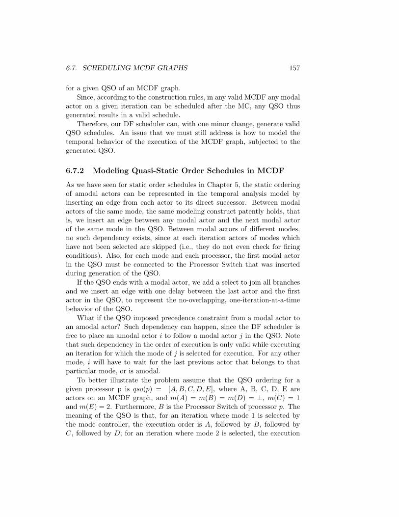
6.7. SCHEDULING MCDF GRAPHS 157
for a given QSO of an MCDF graph.Since, according to the construction rules, in any valid MCDF any modal
actor on a given iteration can be scheduled after the MC, any QSO thusgenerated results in a valid schedule.
Therefore, our DF scheduler can, with one minor change, generate validQSO schedules. An issue that we must still address is how to model thetemporal behavior of the execution of the MCDF graph, subjected to thegenerated QSO.
6.7.2 Modeling Quasi-Static Order Schedules in MCDF
As we have seen for static order schedules in Chapter 5, the static orderingof amodal actors can be represented in the temporal analysis model byinserting an edge from each actor to its direct successor. Between modalactors of the same mode, the same modeling construct patently holds, thatis, we insert an edge between any modal actor and the next modal actorof the same mode in the QSO. Between modal actors of different modes,no such dependency exists, since at each iteration actors of modes whichhave not been selected are skipped (i.e., they do not even check for firingconditions). Also, for each mode and each processor, the first modal actorin the QSO must be connected to the Processor Switch that was insertedduring generation of the QSO.
If the QSO ends with a modal actor, we add a select to join all branchesand we insert an edge with one delay between the last actor and the firstactor in the QSO, to represent the no-overlapping, one-iteration-at-a-timebehavior of the QSO.
What if the QSO imposed precedence constraint from a modal actor toan amodal actor? Such dependency can happen, since the DF scheduler isfree to place an amodal actor i to follow a modal actor j in the QSO. Notethat such dependency in the order of execution is only valid while executingan iteration for which the mode of j is selected for execution. For any othermode, i will have to wait for the last previous actor that belongs to thatparticular mode, or is amodal.
To better illustrate the problem assume that the QSO ordering for agiven processor p is qso(p) = [A,B, C, D, E], where A, B, C, D, E areactors on an MCDF graph, and m(A) = m(B) = m(D) = ⊥, m(C) = 1and m(E) = 2. Furthermore, B is the Processor Switch of processor p. Themeaning of the QSO is that, for an iteration where mode 1 is selected bythe mode controller, the execution order is A, followed by B, followed byC, followed by D; for an iteration where mode 2 is selected, the execution

158 CHAPTER 6. MODE-CONTROLLED DATA FLOW
order is A, B, D, E; for all other iterations, the order is A,a1,a4.To represent the conditional dependency of amodal actor firings on modal
actor firings, we have two options:
1. Interpolation of branches and merges We fix the QSO by in-serting a Select before every amodal actor that appears right after amodal actor in the QSO, except if that actor is a Select, since selectscan merge the schedule. Conversely, every time a modal actor appearsafter an amodal actor in the QSO, we insert before it a Switch tobranch the schedule in modes, except if the actor is a Switch, sinceswitches can branch the schedule. Figure 6.6(a) depicts this way ofmodeling QSO for the previously described example. We omitted theedges from the MC for simplicity sake.
The Processor Switch is the first of the Switches. It marks the pointfrom which the execution of the iteration is dependent on the outputof the MC.
2. “Modalization” of amodal actors. Any amodal actor that appearsafter a Processor Switch in the QSO is replaced by its set of modalcopies, one for each mode. Figure 6.6(b) depict this way of modelingQSO for the previously described example. D1 and D2 are the copiesof actor D, where m(D1) = 1 and m(D2) = 2.
We proceed to explain how an amodal actor can be converted to a setof modal actors. A copy of the amodal actor is created for every modein the MCDF graph. Then, any incoming edge of the original amodalactor is connected to the data input port of a newly created Switch.Each output of this Switch is connected to t the input of the copy ofthe amodal actor associated with the mode of that port. Any outgoingedge of the original amodal actor is connected to the output port ofa newly created Select. Each input port of that select is connected tothe output of the copy of the amodal actor associated with the modeof that port. Figure 6.7 depicts how an amodal actor B with one inputedge and one output edge can be converted to a modal representationon an MCDF graph with two modes. Please note that this conversionmakes each firing of B data-dependent on the firing of the MC on thesame iteration due to the control input of the Switch. The MC andthe edges from MC to the switch and select actors are not depicted.
The conversion of an amodal actor to a modal representation is going tocause the creation of many new switch and select actors and their associatededges in the analysis model.
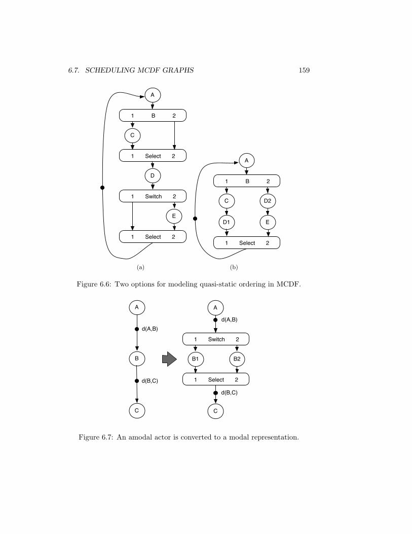
6.7. SCHEDULING MCDF GRAPHS 159
1 B 2
1 Select 2
1 Select 2
1 Switch 2
E
C
D
A
(a)
1 B 2
1 Select 2
E
C
D1
A
D2
(b)
Figure 6.6: Two options for modeling quasi-static ordering in MCDF.
1 Switch 2
1 Select 2
B1
C
A
B2
A
C
B
d(A,B)d(A,B)
d(B,C)
d(B,C)
Figure 6.7: An amodal actor is converted to a modal representation.
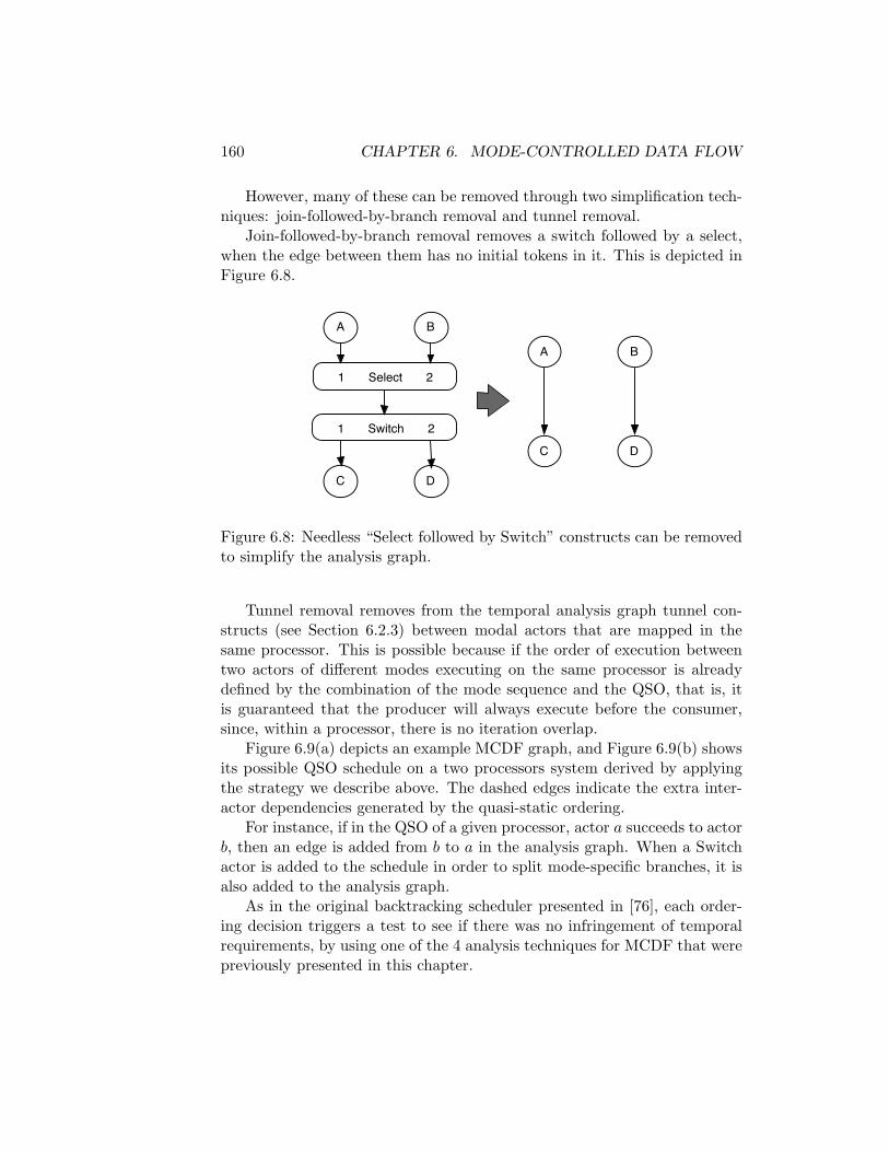
160 CHAPTER 6. MODE-CONTROLLED DATA FLOW
However, many of these can be removed through two simplification tech-niques: join-followed-by-branch removal and tunnel removal.
Join-followed-by-branch removal removes a switch followed by a select,when the edge between them has no initial tokens in it. This is depicted inFigure 6.8.
1 Select 2
A B
1 Switch 2
C D
A B
C D
Figure 6.8: Needless “Select followed by Switch” constructs can be removedto simplify the analysis graph.
Tunnel removal removes from the temporal analysis graph tunnel con-structs (see Section 6.2.3) between modal actors that are mapped in thesame processor. This is possible because if the order of execution betweentwo actors of different modes executing on the same processor is alreadydefined by the combination of the mode sequence and the QSO, that is, itis guaranteed that the producer will always execute before the consumer,since, within a processor, there is no iteration overlap.
Figure 6.9(a) depicts an example MCDF graph, and Figure 6.9(b) showsits possible QSO schedule on a two processors system derived by applyingthe strategy we describe above. The dashed edges indicate the extra inter-actor dependencies generated by the quasi-static ordering.
For instance, if in the QSO of a given processor, actor a succeeds to actorb, then an edge is added from b to a in the analysis graph. When a Switchactor is added to the schedule in order to split mode-specific branches, it isalso added to the analysis graph.
As in the original backtracking scheduler presented in [76], each order-ing decision triggers a test to see if there was no infringement of temporalrequirements, by using one of the 4 analysis techniques for MCDF that werepreviously presented in this chapter.

6.7. SCHEDULING MCDF GRAPHS 161
Mode Switch 1 2 MC
CA
1 2Mode Select
D
Source
B
Sink
(a)
Mode Switch 1 2
MC
CA
1 2Mode Select
DSource B
Sink
Mode Switch 1 2
(b)
Figure 6.9: An MCDF graph and its quasi-static order schedule on twoprocessors.

162 CHAPTER 6. MODE-CONTROLLED DATA FLOW
6.7.3 Determination of Run-Time Scheduler Settings
Run-time scheduler settings can be modeled in a similar way as we describedfor SRDF. If the RTS is a TDM scheduler, then we can simply compute theexecution of the actors in the model exactly as in SRDF. For a round-robinscheduler, it is necessary to remember that the size of the slice is equal tothe maximum sum of execution times across all modes, that is
S(p) = maxm∈M
∑i∈Vmπ(i)=p
t(i). (6.19)
The determination of the RTS settings can be performed by using eitherthe Binary Search Slice Allocator or the Random Slice Allocator, where ateach step the temporal analysis is performed using one of the four methodsdescribed in this chapter.
6.7.4 Determination of Buffer Sizes
With respect to buffer sizing, [10] proved that the problem of finding aschedule that guarantees execution in bounded buffer size is, in general,undecided for a BDF. The same does not apply to our model. As we haveseen, for any MCDF graph, we can generate a rate-equivalent SRDF graphthat assumes conservative bounds on the start times of all actors in theoriginal MCDF graph. Since SRDFs can be executed in bounded bufferspace [81], we know that we can implement our MCDF graphs in boundedbuffer space. Moreover, any of the existing means to compute a throughput-optimal buffer distribution for SRDF graphs[77, 32, 20, 86], will provide asufficient solution for buffer distribution in MCDF for the optimal rate ofthe throughput-equivalent SRDF graph.
For SRDF graphs, we proposed that sufficient buffer sizes could be com-puted by using the linear programming formulation originally described in[77] and corrected by us in [72]. The idea behind that technique to com-pute buffer sizes is that the maximum amount of tokens b(i, j) that needsto be stored in the FIFO corresponding to arc (i, j) ∈ G must be suchthat, between the start of any firing of the producer i and the end of thecorrespondent firing of the consumer j, is lower-bounded by the amount offirings of i that occur in that interval. If the desired maximum period of theexecution is µD, this is given by the inequality
b(i, j) ≥ s(j, k + d(i, j)) + t(j)− s(i, k)µD
(6.20)
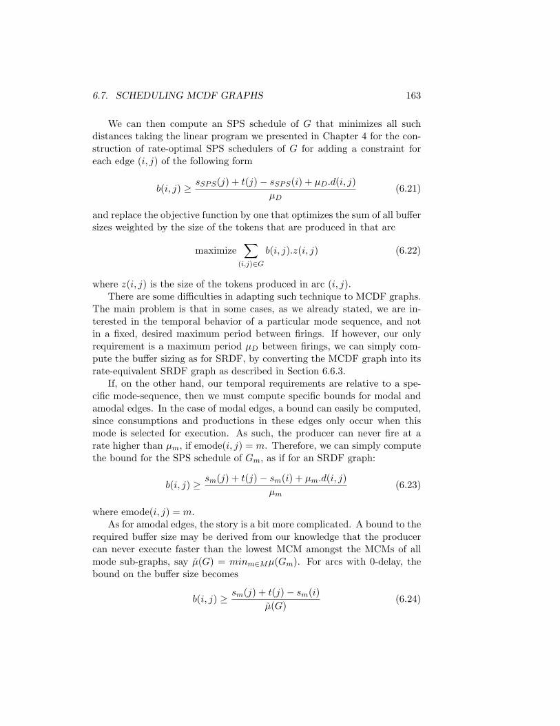
6.7. SCHEDULING MCDF GRAPHS 163
We can then compute an SPS schedule of G that minimizes all suchdistances taking the linear program we presented in Chapter 4 for the con-struction of rate-optimal SPS schedulers of G for adding a constraint foreach edge (i, j) of the following form
b(i, j) ≥ sSPS(j) + t(j)− sSPS(i) + µD.d(i, j)µD
(6.21)
and replace the objective function by one that optimizes the sum of all buffersizes weighted by the size of the tokens that are produced in that arc
maximize∑
(i,j)∈G
b(i, j).z(i, j) (6.22)
where z(i, j) is the size of the tokens produced in arc (i, j).There are some difficulties in adapting such technique to MCDF graphs.
The main problem is that in some cases, as we already stated, we are in-terested in the temporal behavior of a particular mode sequence, and notin a fixed, desired maximum period between firings. If however, our onlyrequirement is a maximum period µD between firings, we can simply com-pute the buffer sizing as for SRDF, by converting the MCDF graph into itsrate-equivalent SRDF graph as described in Section 6.6.3.
If, on the other hand, our temporal requirements are relative to a spe-cific mode-sequence, then we must compute specific bounds for modal andamodal edges. In the case of modal edges, a bound can easily be computed,since consumptions and productions in these edges only occur when thismode is selected for execution. As such, the producer can never fire at arate higher than µm, if emode(i, j) = m. Therefore, we can simply computethe bound for the SPS schedule of Gm, as if for an SRDF graph:
b(i, j) ≥ sm(j) + t(j)− sm(i) + µm.d(i, j)µm
(6.23)
where emode(i, j) = m.As for amodal edges, the story is a bit more complicated. A bound to the
required buffer size may be derived from our knowledge that the producercan never execute faster than the lowest MCM amongst the MCMs of allmode sub-graphs, say µ(G) = minm∈Mµ(Gm). For arcs with 0-delay, thebound on the buffer size becomes
b(i, j) ≥ sm(j) + t(j)− sm(i)µ(G)
(6.24)

164 CHAPTER 6. MODE-CONTROLLED DATA FLOW
for all modes m ∈ M such that emode(i, j) = m or emode(i, j) = ⊥. Ifd(i, j) 6= 0, then we again have the same problem we encountered withrespect to temporal analysis, ie, that the execution of a previous iteration ofan actor is subject to the dependencies of a different mode sub-graph and,therefore to a different rate. In that case, we use the same expedient asbefore, where we convert the input graph such that for all edges the delayis one or 0, and we now have to consider as a bound on the buffer size themaximum bound amongst all the possible mode transitions
b(i, j) ≥ maxm∈Mn∈M
(sm(j) + κnm + t(j)− sn(i)
µ(G)) (6.25)
We can now, given an MCDF graph, compute sufficient buffer size bysimply computing first the MCMs for all mode sub-graphs, then all SPSsfor all the mode sub-graphs, then all the transition intervals, then all thebounds for the buffer sizes of all arcs, and then, per arc, take the lowestinteger value that respects those bounds.
6.8 Scheduling Experiments
We applied our MCDF scheduling flow to the WLAN receiver depicted inFigure 6.5, mapped to the same heterogeneous multiprocessor we used asa platform in Chapter 5. We ran the MCDF graph of the WLAN throughthe scheduling flow for 2 different mode sequences: one for the shortestpossible packet, i.e. a mode sequence where the synchronization mode runstwice, the header mode once, and the payload mode once, and another forthe longest packet, i.e. the same as the previous, except that the payloadmode runs 256 times. We used both the SPS-based analysis and simulation-based analysis for constraint verification. The results are presented in Tables6.1, 6.2, 6.3, 6.4. In these tables, the highest priority is 3 and the lowestpriority is 1. We expected to find that the overestimation of the executiontime of the sequence with SPS-based analysis would cause final slice sizesto be larger that for simulation-based analysis, and that was indeed thecase. We expected the worst overestimation to occur for the small sequence,as the main overestimation is caused at the start of execution of a mode,and during transitions, and the the proportional contribution on the smallsequence of transitions is much larger than for the long sequence, that staysin the payload mode for 256 consecutive iterations. This was verified bythe experiment. The largest difference in required resource utilization afterscheduling and slice size determination was found for the short sequence,
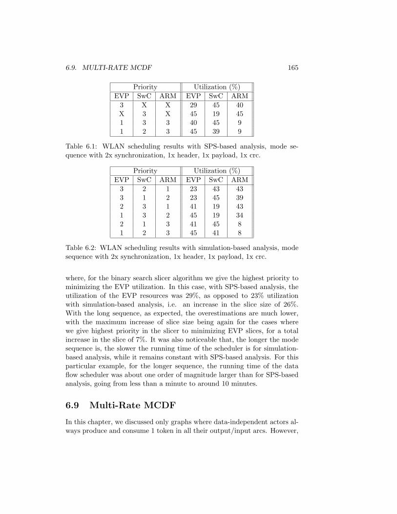
6.9. MULTI-RATE MCDF 165
Priority Utilization (%)EVP SwC ARM EVP SwC ARM
3 X X 29 45 40X 3 X 45 19 451 3 3 40 45 91 2 3 45 39 9
Table 6.1: WLAN scheduling results with SPS-based analysis, mode se-quence with 2x synchronization, 1x header, 1x payload, 1x crc.
Priority Utilization (%)EVP SwC ARM EVP SwC ARM
3 2 1 23 43 433 1 2 23 45 392 3 1 41 19 431 3 2 45 19 342 1 3 41 45 81 2 3 45 41 8
Table 6.2: WLAN scheduling results with simulation-based analysis, modesequence with 2x synchronization, 1x header, 1x payload, 1x crc.
where, for the binary search slicer algorithm we give the highest priority tominimizing the EVP utilization. In this case, with SPS-based analysis, theutilization of the EVP resources was 29%, as opposed to 23% utilizationwith simulation-based analysis, i.e. an increase in the slice size of 26%.With the long sequence, as expected, the overestimations are much lower,with the maximum increase of slice size being again for the cases wherewe give highest priority in the slicer to minimizing EVP slices, for a totalincrease in the slice of 7%. It was also noticeable that, the longer the modesequence is, the slower the running time of the scheduler is for simulation-based analysis, while it remains constant with SPS-based analysis. For thisparticular example, for the longer sequence, the running time of the dataflow scheduler was about one order of magnitude larger than for SPS-basedanalysis, going from less than a minute to around 10 minutes.
6.9 Multi-Rate MCDF
In this chapter, we discussed only graphs where data-independent actors al-ways produce and consume 1 token in all their output/input arcs. However,
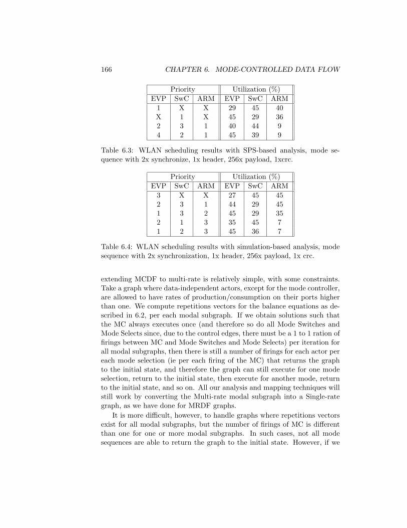
166 CHAPTER 6. MODE-CONTROLLED DATA FLOW
Priority Utilization (%)EVP SwC ARM EVP SwC ARM
1 X X 29 45 40X 1 X 45 29 362 3 1 40 44 94 2 1 45 39 9
Table 6.3: WLAN scheduling results with SPS-based analysis, mode se-quence with 2x synchronize, 1x header, 256x payload, 1xcrc.
Priority Utilization (%)EVP SwC ARM EVP SwC ARM
3 X X 27 45 452 3 1 44 29 451 3 2 45 29 352 1 3 35 45 71 2 3 45 36 7
Table 6.4: WLAN scheduling results with simulation-based analysis, modesequence with 2x synchronization, 1x header, 256x payload, 1x crc.
extending MCDF to multi-rate is relatively simple, with some constraints.Take a graph where data-independent actors, except for the mode controller,are allowed to have rates of production/consumption on their ports higherthan one. We compute repetitions vectors for the balance equations as de-scribed in 6.2, per each modal subgraph. If we obtain solutions such thatthe MC always executes once (and therefore so do all Mode Switches andMode Selects since, due to the control edges, there must be a 1 to 1 ration offirings between MC and Mode Switches and Mode Selects) per iteration forall modal subgraphs, then there is still a number of firings for each actor pereach mode selection (ie per each firing of the MC) that returns the graphto the initial state, and therefore the graph can still execute for one modeselection, return to the initial state, then execute for another mode, returnto the initial state, and so on. All our analysis and mapping techniques willstill work by converting the Multi-rate modal subgraph into a Single-rategraph, as we have done for MRDF graphs.
It is more difficult, however, to handle graphs where repetitions vectorsexist for all modal subgraphs, but the number of firings of MC is differentthan one for one or more modal subgraphs. In such cases, not all modesequences are able to return the graph to the initial state. However, if we

6.10. RELATED WORK 167
require the MC to behave such that for all valid mode sequences, each modeis selected a number of times equal to the number of repetitions of the MC onthe repetitions vector of the modal subgraph for each mode, then the graphis still guaranteed to be able to fire in such a way as to return to the initialstate after each sequence of firings of the same mode, and it is reasonableto assume that all analysis and mapping techniques can still be adapted tohandle such graphs. This however, should be the subject of further study.
6.10 Related Work
We have already discussed the limitations of Static Data Flow variants andof Integer Data Flow both in Chapter 3 and in the introduction of thischapter. During the last few years, however, there have been attempts insome ways similar to ours to find a better balance between expressivity andanalytical properties. In such category falls the work on Variable-PhasedData Flow (VPDF) presented in [92]. With VPDF, actors cycle through alist of execution phases determined at compile time. The variable runtimebehavior comes from the fact that each phase can be fired a number oftimes dependent on data values that can only be known during execution.Conditional behavior can be represent since phases can execute 0 or moretimes depending on data values. In [92] it is shown how, by knowing themaximum number of executions per phase, one can compute buffer sizesfor a VPDF graph to meet a given throughput requirement. Scheduling isassumed to be dynamic, and no techniques have been proposed for staticor quasi-static ordering of actors, nor, for that matter, any way of takingmapping decisions beside buffer sizing either at compile time or run time
Another approach, much closer to ours, is taken in the work on Scenario-Aware Data Flow (SADF), first introduced in [89]. In [23], a technique isprovided for real-time analysis of SADF graphs. In SADF, an applicationis modeled as a collection of SDF graphs, each representing individual sce-narios of behavior, and a Finite State Machine (FSM) that specifies thepossible orders of scenario occurrences. The paper provides techniques toanalyze worst-case performance of such applications. These techniques candetermine the highest throughput that can be guaranteed and can determinethe minimal latency that can be attained from a state space analysis. SADFis very similar to MCDF in many ways. In fact, according to preliminaryresults of a study which was still being carried out at the time of the writingof this thesis, it is very likely that the two models have the same expressivepower and that an automatic conversion between the two is possible. The

168 CHAPTER 6. MODE-CONTROLLED DATA FLOW
analysis techniques for SADF require the same information that we use forMCDF analysis: a graph per mode/scenario and a specification of scenariotransitions of interests. In our case, this is done with the specification ofmode sequences; in SADF, with the specification of a finite state machine forscenario transitions. The analysis technique proposed for SADF requires theexhaustive analysis of the state space of the execution of the SADF graph,as specified by the FSM. Our usage of reference schedules makes the analysisless precise, but avoids an exhaustive search space exploration, which is alsoa problem we have with the analysis technique where we apply data flowsimulation for all mode sequences of interest.
A difference between MCDF and SADF is that SADF was primarilydesigned as a way of modeling behavior and not as a programming modeland, because of that, the execution model is not explicit about the relationbetween scenario transition decisions and data flow execution, i.e., if onedefines the FSM and each one of the graphs per scenario, there is still noway of knowing where the decision to go from one scenario to another wastaken. Application mapping techniques for SADF were proposed in [87]. Inthis work, static ordering is handled by a single attempt, heuristic algorithmthat assumes that the mode of execution is known from the start of theiteration at each processor. It is not clear how this constrains the optionsavailable to the scheduler. Due to the similarity between SADF and MCDF,it is very likely that MCDF mapping techniques can be applied to SADFgraphs.
6.11 Conclusions
Transceivers are mostly iterative, repetitive applications, with little datavalue-dependent behavior. However, the little data value-dependent behav-ior there is cannot easily be accommodated by the static data flow computa-tion models. This posed a serious problem, as, until recently, only the staticflavors of data flow were known to have the analytical properties that allowsus to guarantee hard-real time behavior. On one side we had the dynamicdata flow variants that could not be analyzed, and on the other side we hadthe static data flow models that we could analyze, but were not expressiveenough to model the behavior of transceivers. The work presented in thischapter tried to find a compromise: we allowed for a small amount of data-dependent behavior and extended the known analysis techniques for staticgraphs to accommodate for this small amount of dynamism. The result wasthe Mode-Controlled Data Flow computation model. We have shown how

6.11. CONCLUSIONS 169
MCDF can be analyzed in terms of minimum guaranteed throughput andmaximum latency bound and we have extended the techniques for applica-tion mapping we developed in Chapter 5 so that MCDF graphs representingradio applications can be quasi-statically scheduled onto multiprocessor sys-tems.
There is still work to be done. Our quasi-static ordering scheduler is anadaptation of our static ordering scheduler, and, as such, it still makes anexhaustive search for feasible schedules, with an algorithm of exponentialcomplexity. For buffer sizing, we have only shown that we can compute anupper bound to the requirements, but this upper bound is not optimal inany sense.
The biggest challenge, however, is probably the expressivity of the model.The expressivity of MCDF was chosen such that the transceivers that wereknown to us could be conveniently expressed. There is a trend, however, forbaseband processing to become more irregular, with more complex control,as can be seen in the evolution of 4G standards such as LTE. It is yet tobe seen whether MCDF can cope with the increase of control complexity inbaseband processing. At the time of writing, a study has been carried outto model LTE in MCDF and MCDF seems to be capable to express all therequired behavior, but the complexity of the data flow model thus obtainedalso points towards the need for multi-rate and cyclo-static constructs, aswell as more constructs such as the Mode Tunnel that, although reducibleto Mode Switches and Selects, will make the specification of radios simpler.
It is also yet to see what lessons can be learned and what techniques canbe adopted from the work on SADF and VPDF.

170 CHAPTER 6. MODE-CONTROLLED DATA FLOW

Chapter 7
Resource Manager
In this chapter, we will discuss the algorithms that the resource managermust implement to try to find a mapping for a transceiver instance (a job)at runtime, and decide whether the job can be executed or not.
In the previous chapters, we have seen how a transceiver described bya data flow graph can be prepared at compile time for runtime allocationof resources. Actors are first bundled into quasi-statically ordered clusters.Each cluster is annotated with a resource budget, which includes schedulersettings (the size of a slice per period) and memory requirements, whilecommunication channels between clusters are annotated with required buffercapacity.
As already sketched in Chapter 2, our approach to the resource man-agement problem for a system with dynamic job-set and job-mix is to givejobs a degree of independence from the rest of the system by using a strongresource management policy. The resource management policy should en-sure: a) admission control – a job is only allowed to start if the system canallocate upon request the resource budget it requires to meet its timing re-quirements; and b) guaranteed resource provisions – the access of a runningjob to its allocated resources cannot be denied by any other job. Resourcebudgets are computed offline such that jobs meet timing constraints, usingthe techniques guided by temporal analysis that we described in Chapter 5.
As we have argued in Chapter 2, the enforcement of resource budgetsrequires the hardware platform to provide predictable arbitration schemes,that is, arbitration schemes that allow us to tightly bound the time that arequest takes to be served.
We designed a template for scalable multiprocessor architectures thatfits these requirements. We use global resource allocation to implement
171

172 CHAPTER 7. RESOURCE MANAGER
admission control and local schedulers to guarantee resource provision. Asimplified version of this architecture was presented in Chapter 2. In thischapter, we extend the communication infrastructure by using an ÆtherealNetwork-on-Chip [29]. Æthereal fits well in this architecture template asit allows for resource reservation by providing connections with guaranteedminimum throughput and maximum latency.
We start our discussion assuming a target platform containing a TDM-arbitrated router– i.e. an Æthereal network with a single router – for inter-tile communications. We show that the problem can be seen as a gener-alization of Vector Bin-Packing (VBP) [54] and, since the problem is NP-complete, provide heuristic approaches to tackle it. Since a single routerarchitecture does not scale with an increase in the number of cores, we lookat the problem assuming a network with many (4 to 12) routers.
By adding the network, the system changes in two important aspects.First, the resource allocator must find routes through the network and re-serve time slots per link per router. Secondly, the network cannot be mod-eled as a single resource, as bottlenecks between two tiles are formed de-pending on which routes are allocated. Special care has to be taken aboutwhich processors are used for which tasks, even though the set of processorsitself is homogeneous.
In Section 7.1, we explain how this work relates to the work of others.In Section 7.2, we describe the assumptions about hardware, software andscheduling mechanisms that were used in this study. In Section 7.3 weformally model the resource allocation problem. In Section 7.4, we describesthe heuristics we propose to find a feasible allocation. In Section 7.5 wedescribe our experiments and results. Finally, we state the conclusions forthis chapter in Section 7.6.
7.1 Related Work
An extensive survey or the traditional techniques for scheduling and resourceallocation in embedded multiprocessors can be found in [82]. It describestechniques from fully static to fully dynamic scheduling. However, it doesnot consider the case in which tasks arrive and leave at runtime, as in ourcase. The same holds for techniques that compute task assignments atdesign-time, such as [91].
In CPA [67], it is considered that jobs may start and stop at any time.Each job mix has its own schedule, which is calculated at compile time andstored in a look-up table. This approach is not without problems. The

7.2. SYSTEM ARCHITECTURE 173
number of potential job combinations is exponential in the number of jobs,and switching from one configuration to the other could mean a non-trivialprocessor migration of running tasks. Moreover, it assumes that all tasksare known at compile time.
The literature on task allocation for tasks with a periodic requirementis extensive, and covers many combinations of constraints. Previous ap-proaches either do not consider any network [4, 59, 30, 63, 95], consider onlya bus topology [5], require tasks to be migratable between processors [30],or require a solution to be computed at compile time [67, 91]. Hansson etal. [40] consider the network, but do an off-line computation of the networkslot tables, provided the assignment of tasks to processors is given. Ourapproach does not share these restrictions. We do task assignment usingglobal system knowledge. Task to processor assignment is done at job starttime. Task scheduling is done locally on the processor and it can use anypredictable scheduling mechanism such as Non-Preemptive Non-BlockingRound-Robin or TDM.
In [66], the authors propose a technique similar to ours to model thenetwork-on-chip resources as a graph where each node corresponds to a slicein each one of the routers, and each edges corresponds to a link. This work,however, does not consider processor allocation, assuming it is given a priori.
7.2 System Architecture
In this section we will describe some relevant aspects of the type of systemwe consider. We will describe the hardware and software models, as well asthe scheduling mechanisms used in the processors.
7.2.1 Hardware
In Chapter 2 we propose a hardware architecture consisting of a set of pro-cessors, of different types, fully connected through a global communicationframework. In this chapter, we will both simplify and extend this model.First, we will consider a homogeneous system, i.e. all processors are of thesame type. The reason for this is that, since in our framework each taskcan only run in one specific type of processor, the problem of allocatingresources to such a task is restricted to finding a processor of the type thattask requires. The problem of resource allocation for our heterogeneous sys-tem can therefore be seen as jointly solving the resource allocation problemfor several homogeneous multiprocessor systems.

174 CHAPTER 7. RESOURCE MANAGER
On the other hand, we have not described in Chapter 2 in detail whatthe communication infrastructure looks like. If for relatively small simplearchitectures a multi-layer bus may suffice (provided that care is taken toemploy predictable slave-side arbiters) such a solution will not scale wellwith an increase in the number of cores in the architecture.
In this chapter, the hardware under consideration consists of a homo-geneous set of processors, connected through a network of routers. Theprocessors and the network are placed on a single chip, forming a Multi-Processor System on Chip. We will consider at most 24 processors and 12routers.
Each processor resides on its own processing tile (PT), which consistsof a processor, local memory (MEM), a communication assist (CA) and anetwork interface (NI). The CA offers a fixed number of time slices that itallocates to memory accesses between the ARM and the NI. The NI offersa fixed number of input/output FIFO queues for accessing the channelsallocated over the network.
Figure 7.1: A processing tile.
For a model of the network we consider the Æthereal [30, 29] Network-on-Chip. The Æthereal can use contention-free routing, based on TDMswitching and allows links with guaranteed throughput and latency. Everyrouter is connected to other routers and/or to NIs. Each PT has one singleNI. Due to physical constraints, the routers can have at most 8 bidirectionalconnections. Every connection consists of a fixed number of links, and eachlink offers a fixed amount of bandwidth.
Data are transmitted by the routers in three-words packets. All routersand tiles send and receive data packets synchronously as if operating undera global clock. If data arrives on an input at tick t, it will be sent throughthe router to the output link and arrive at the other end of that link at tick

7.2. SYSTEM ARCHITECTURE 175
t+1. Per time slice, a packet from each input link is sent to an output link,according to a slot reservation table that specifies per time slice which inputlink is connected to each output link.
Two processes on different PTs can communicate unidirectionally byestablishing a channel. This requires a send and a receive buffer to beallocated in the data memory of their respective PTs, as well as time slices inthe CA and queues in the NI on both sides. In the network, a communicationchannel must be created by finding a path across routers from source PT todestination PT. The routers do not buffer their input packets. Therefore,when a packet arrives to an input link in a router, it must be sent at theend of the cycle to the output link specified for that time slot in the slotreservation table.
Each processor runs either a TDM or a NPNBRR scheduler, and has a(possibly empty) set of tasks assigned to it.
7.2.2 Application
As in previous chapters, we will assume that the application consists of anumber of stream-processing jobs. An unpredictable source, such as theuser, can ask to start or stop a job instance at any moment. Because theuser can typically request for more job instances than the hardware can runsimultaneously, there is a resource allocation problem. If the system canfind sufficient resources, the job is started. Otherwise, the user is informedof the lack of resources, and the system refuses to start the job.
The jobs are modeled as directed graphs. Nodes represent computationtasks, and edges represent FIFO communication channels. These graphsare not data flow graphs of the same type used in previous chapters. Infact, after our compile time scheduling techniques have been applied to adata-flow graph, a new graph has been generated: each task in this graphcorresponds to a cluster of actors (quasi-)statically ordered and annotatedwith budget requirements such as scheduler settings (for a TDM scheduler,this is processor cycles per TDM period) and memory consumption for bothdata and instructions.
Channels require memory space to store buffers, as well as network band-width. We did not discuss how to compute the bandwidth requirements ofchannels in Chapter 5, as we assumed that communication between actorswas accounted for as remote stores by the producers into buffer spaces re-served at the side of the consumer. In this chapter, due to the introductionof the network, we can no longer make such an assumption, and thereforean explanation is required on where and how such bandwidth budgets can

176 CHAPTER 7. RESOURCE MANAGER
cR jcLi
(a)
nR nHnLi j
(b)
nR nHnL
i
j
cR1cL1
cR2cL2
(c)
Figure 7.2: Data flow models for a) Communication Assist link b) Networklink c) channel from producer to consumer in different PTs.
be derived.
Determining bandwidth budgets for channels
With the introduction of the communication assists and the Æthereal net-work, communication now requires reservation of communication resources.
In terms of the temporal analysis model, a channel between two single-rate actors i and j through a producer-side CA, a number of network routersand a consumer-side CA can be represented by replacing the arc between(i, j) by a latency-rate server data flow models connected in series: a modelfor the producer-side CA, followed by a model for the network and a modelfor the consumer-side CA. The CAs are represented each by a latency-rateserver model (depicted in Figure 7.2(a)). The network is represented by asingle latency-rate server component followed by an actor that models thelatency caused by the synchronous transfer of packets through subsequentrouters on the path, as explained in the previous section (depicted in Figure7.2(b)). The complete model of the temporal behavior of a channel (i, j)implemented over the network is shown in Figure 7.2(c).
These models are parametric. The execution times of the two actors

7.2. SYSTEM ARCHITECTURE 177
cL and cR in the CA model are given respectively by t(cL) = (NCA −BCA(i, j)).PCA where PCA is the period of the CA time wheel (we as-sume TDM arbitration on the communication assist), NCA is the fixed num-ber of equally-sized slices per period that the CA scheduler provides, andBCA(i, j) is the number of slices allocated for link (i, j) in the CA, andt(cR) = z(i,j)
BCA(i,j).wCA.PCA, where z(i, j) is the size in words of the tokens
produced by i and consumed by j and wCA is the number of words the CAcan transfer per slice.
The execution times of the three actors nL, nR and nH that represent thenetwork are given by t(nL) = (NNet−BNet(i, j)).PNet, t(nR) = z(i,j)
BNet(i,j).wNet,
and t(nH) = (h(i, j) − 1) PNetNNet
, where PNet is the period the time wheel ofeach network router, NNet is the fixed number of equally-sized slices perperiod that each network router provides, BNet(i, j) is the number of slicesper period allocated to link (i, j) in a network router (it must be the same forall network routers that the connection provided to channel (i, j) traverses,and h(i, j) is the number of network routers that each packet sent throughchannel (i, j) must traverse.
If we assume a worst case for h(i, j) = h, where h is the number ofrouters in the network, i.e. we assume that each channel may traverse allrouters once, and we explicitly disallow a channel from traversing the samerouter twice, then all parameters in the model are application independent,except for the BCA(i, j) and BNet(i, j) parameters, which represent the CAand network bandwidth budgets of channel (i, j). Since in an SRDF grapheach producer produces at most once per period, and assuming that µD ≥PNet, then can simply set the required bandwidth to z(i, j) words per µD,which means that BNet(i,j)
PNet≥ z(i,j)
µDwhich implies that BNet(i, j) ≥ z(i,j).PNet
µD.
Assuming that a low latency is not necessary, we can set budget BNet(i, j)to be equal to this lower bound (same formulas and conclusion can be drawnfor BCA(i, j) budgets). If temporal analysis indicates that assuming valuesthus obtained creates an unfeasibility of throughput or latency requirements,then the budgets can be increased. Channel bandwidth budgets “withdraw”from the same deadline extension pools as the slicing optimization phase ofthe compile time scheduler, and the same methods as were described inChapter 5 can be used to determine instead or in combination with TDMslices for processor schedulers.
178 CHAPTER 7. RESOURCE MANAGER
7.3 Resource Allocation
If a request to start a job arrives, sufficient resources need to be found andallocated for its tasks and channels. The tasks are to be allocated to PTs,and routes need to be allocated in the network for the channels betweentasks on different PTs.
The problem is to find such an allocation, while trying to keep as manyfree resources as possible for jobs that may be started later. Also, it is aconcern that computing resources may start fragmenting across the platformafter many job starts and stops.
We first give a simplified example to highlight some of the challengesinvolved in solving the allocation problem. Then, we will describe how weformally model resource providing and resource requesting entities. We thenformally define the allocation problem, discuss its complexity and strategieson how to solve it.
7.3.1 Motivating Example
The three jobs depicted in Figure 7.3(a) are to be placed simultaneously ontothree empty tiles. We assume a single-router network, and can therefore ig-nore for now the problems related with network topology. To illustrate thetrade-offs involved, we depict several different allocations in Figure 7.3(b). Inthis example, for the sake of simplicity, each task in a job requires only com-putational resources and each tile provides only computational resources.Placement strategy 1 tries to map the whole job onto a new processor tominimize communication costs. This strategy fails to find a feasible allo-cation by requiring four processors to be used instead of three. Placementstrategy 2 packs the tasks as tightly as possible and concentrates all the freespace in a single processor. Jobs are now scattered over the processors, lead-ing to high communication costs between tasks. If we rearrange the tasks,as shown in strategy 3, we lower the communication overhead, while keep-ing the same distribution of free space. Packing strategy 4 shows anotherpossible free space vs. communication trade-off. It reduces the amount ofinter-processor communication at the expense of fragmenting the remainingcomputing resources.
7.3.2 PT Resource Provision
A PT provides computation, memory and communication resources. Thiscan be represented as a resource provision vector. If p is a PT, then the re-
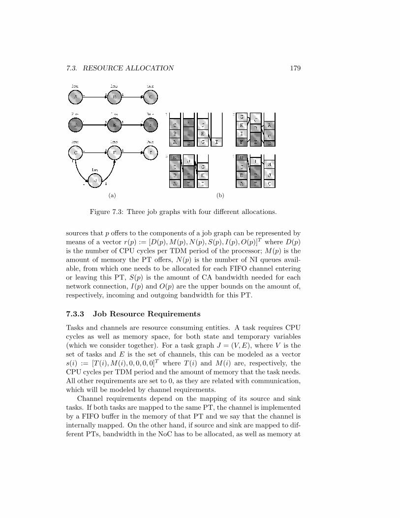
7.3. RESOURCE ALLOCATION 179
(a) (b)
Figure 7.3: Three job graphs with four different allocations.
sources that p offers to the components of a job graph can be represented bymeans of a vector r(p) := [D(p),M(p), N(p), S(p), I(p), O(p)]T where D(p)is the number of CPU cycles per TDM period of the processor; M(p) is theamount of memory the PT offers, N(p) is the number of NI queues avail-able, from which one needs to be allocated for each FIFO channel enteringor leaving this PT, S(p) is the amount of CA bandwidth needed for eachnetwork connection, I(p) and O(p) are the upper bounds on the amount of,respectively, incoming and outgoing bandwidth for this PT.
7.3.3 Job Resource Requirements
Tasks and channels are resource consuming entities. A task requires CPUcycles as well as memory space, for both state and temporary variables(which we consider together). For a task graph J = (V,E), where V is theset of tasks and E is the set of channels, this can be modeled as a vectors(i) := [T (i),M(i), 0, 0, 0, 0]T where T (i) and M(i) are, respectively, theCPU cycles per TDM period and the amount of memory that the task needs.All other requirements are set to 0, as they are related with communication,which will be modeled by channel requirements.
Channel requirements depend on the mapping of its source and sinktasks. If both tasks are mapped to the same PT, the channel is implementedby a FIFO buffer in the memory of that PT and we say that the channel isinternally mapped. On the other hand, if source and sink are mapped to dif-ferent PTs, bandwidth in the NoC has to be allocated, as well as memory at

180 CHAPTER 7. RESOURCE MANAGER
both extremities, outgoing/incoming bandwidth, network interfaces and CAbandwidth. We say that such a channel is externally mapped. The vectorthat represents the resource consumption of an internally mapped channel is:i(e) := [0,M(e), 0, 0, 0, 0]T , where M(e) is the amount of memory requiredto store the FIFO relative to channel e. If the edge is externally mapped,resources are required from both the source tile and the sink tile. This canbe expressed by two vectors, p(e) and c(e), representing respectively theresource usage at source and sink PTs p(e) := [0,Mp(e), 1, Cp(e), 0, b(e)]T ,c(e) = [0,Mc(e), 1, Cc(e), b(e), 0]T , where b(e) is the bandwidth required bythe channel, Mp(e) and Mc(e) are, respectively, the memory required tostore the source and sink endpoints, and Cp(e) and Cc(e) represent the CAbandwidth required.
These four resource requirement vectors can be reduced to two by thefollowing transformation. Let w(i) be the amount of resources needed tohost task i, i.e.,
w(i) := s(i) +∑
e=(i,b)∈E
p(e) +∑
e=(b,i)∈E
c(e).
The resources that are saved when both endpoints of a channel are mappedto the same PT is modeled by
δ(e) := p(e) + c(e)− i(e).
Then, a set of tasks A can be allocated on PT p iff:∑a∈A
w(a)−∑
e=(a,b)∈Ea∈A,b∈A
δ(e) ≤ r(p). (7.1)
7.3.4 Network Resource Provision
The route through which the packets of a FIFO channel flow through thenetwork should be allocated, and is fixed for the lifetime of the channel itsupports. Such a route through the network consists of a path through therouters used and slot allocations for the slot reservation tables of each oneof the routers.
In previous work [40], path finding and slot reservation in NoC resourceallocation are decoupled: first a path is found in a directed graph model ofthe network where nodes are routers and edges are links between routers,and given such a path, an attempt is made to do the slot allocation. If theslot allocation fails, then a new path is searched for.
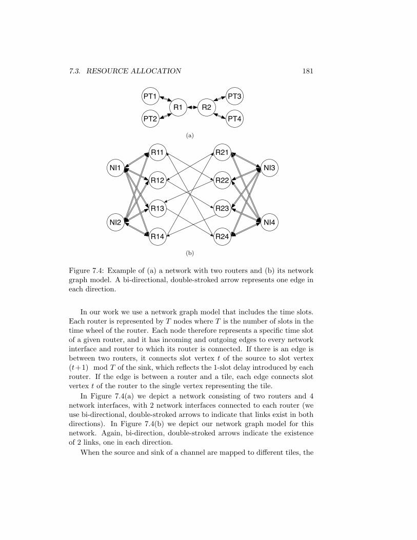
7.3. RESOURCE ALLOCATION 181
R2PT3
R1PT2
PT1
PT4
(a)
R13
R12
R11
R14 R24
R23
R22
R21
NI1
NI2
NI3
NI4
(b)
Figure 7.4: Example of (a) a network with two routers and (b) its networkgraph model. A bi-directional, double-stroked arrow represents one edge ineach direction.
In our work we use a network graph model that includes the time slots.Each router is represented by T nodes where T is the number of slots in thetime wheel of the router. Each node therefore represents a specific time slotof a given router, and it has incoming and outgoing edges to every networkinterface and router to which its router is connected. If there is an edge isbetween two routers, it connects slot vertex t of the source to slot vertex(t+1) mod T of the sink, which reflects the 1-slot delay introduced by eachrouter. If the edge is between a router and a tile, each edge connects slotvertex t of the router to the single vertex representing the tile.
In Figure 7.4(a) we depict a network consisting of two routers and 4network interfaces, with 2 network interfaces connected to each router (weuse bi-directional, double-stroked arrows to indicate that links exist in bothdirections). In Figure 7.4(b) we depict our network graph model for thisnetwork. Again, bi-direction, double-stroked arrows indicate the existenceof 2 links, one in each direction.
When the source and sink of a channel are mapped to different tiles, the

182 CHAPTER 7. RESOURCE MANAGER
channel requires a route through the network to be allocated between thesetwo tiles. In the network graph model, this corresponds to finding a set ofpaths between the two NIs of those tiles, which together provide enoughbandwidth to support the channel. In this way, finding a path throughthe network and a slot allocation become a single problem. The trade-offis, of course, that if the original network had R routers and L links, thecorresponding graph in the traditional model has R nodes and L edges, ournetwork graph model has T ×R nodes and T × L edges.
For the whole job, more than one route will typically be allocated throughthe network. Because in every time slice a router can only route to each out-put link a single input link, these paths are not allowed to collide, i.e. toshare edges. Finding several paths in the network graph model that do notcollide amounts to solving the Directed Edge-Disjoint Paths Problem, whichis NP-complete even in many restricted cases [53]. Instead of solving it di-rectly by considering all paths at once, we can approximate a solution byfinding routes one at a time using Shortest Path. In theory, this algorithmis capable of finding at least a fraction of Ω(1/
√|E0|) of the routes possible,
where |E0| is the number of channels allocated in an optimal solution [51].In practice however, it usually performs much better.
7.4 Mapping Jobs
The problem of mapping a single job to the target platform can be formu-lated in this way:
Problem 1. Single Job Resource Allocation : Given a job digraphG = (V,E), and a network topology digraph T = (P ∪ R,N) of processingtiles P , router nodes R and network links N . Also given a weight b(e) > 0for each edge in E, representing the amount of bandwidth capacity requiredby channel e. The topology T is restricted by the fact that each vertex in P isonly connected to exactly one router in R (assuming |P | > 1). Besides that,P has a valuation r : P → N6, the resource provision of p, and all n elementsof V have valuation w : V → N6, the resource usage of n, and all e elementsof E have valuation δ : E → N6, the resource savings for internal mappingof e. Does there exist an injective mapping m of tasks V to tiles P such thatthere exist edge-disjoint paths through the network (through R and N nodes)to accommodate the edges between the tasks in the mapping, knowing thateach edge e requires b(e) paths from the tile m(src(e)) to the tile m(snk(e)),where src(e) is the source task of e and snk(e) is the destination task of e,

7.4. MAPPING JOBS 183
while guaranteeing that for all tiles p it holds that∑n∈A(p)
w(n)−∑
e=(n,v)∈En∈A(p),v∈A(p)
δ(e) ≤ r(p), (7.2)
where A(p) = n ∈ V : m(n) = p, is the set of tasks mapped to tile p?
This problem is NP-complete. We will proceed to show this in twosteps: 1) show that the problem is in NP, that is, a solution can be verifiedin polynomial time, and 2) show that all the instances of a known NP-hard problem are an infinite subset of the set of instances of our problem.1) Checking whether a given mapping solves 1 can be done in polynomialtime: first, per PT, calculate the total unmodified resource consumptionby summing the resource requirements w(n) of all nodes mapped to thatPT; then, for each edge, check if its endpoints are in the same PT, and,if so, adjust resource consumption in that PT according to δ(e); for eachPT P , check if the total resource consumption is less than r(p). This hasa complexity of O(N2). Check for each externally mapped edge whetherthe route exists. This has a maximum complexity O(N) for a given fixednumber of routers and slices per router in the network. 2) Any instanceof off-line Vector Bin-Packing (VBP) can be reduced to an instance of ourproblem where items become nodes, bins become PTs and the edge set isempty. In all instances of Problem 1 where there are no edges, the sumof δ(e) in the problem formulation becomes zero in all dimensions, and theformulation of Problem 1 becomes equivalent to the formulation of VBP.Therefore a positive of VBP will be a positive of Problem 1 and vice-versa.Problem 1 is thus NP-complete.
We must also take into consideration that the solution cannot be algo-rithmically complex, because the resource manager must run on-line. Theproblem resembles the Vector Bin-Packing (VBP) problem by viewing thePTs as bins and the tasks as items. The resources provided by the PTs andthe resources required by the tasks become the bin capacities and item sizes,respectively. However, there are non-trivial differences between our problemand VBP. In VBP, the items to be packed have a constant size, while in ourresource allocation problem, the resources required by the endpoints of achannel depend on whether or not they are mapped to the same PT. Thiscan be disregarded, but that would over-dimension the problem. Also, VBPdoes not take bandwidth usage into account, nor the available routes in thenetwork.
Our experiments in Section 7.5.1 will show that, for a 1-router systemwhere topology is not an issue, the low-complexity First-Fit (FF) and First-

184 CHAPTER 7. RESOURCE MANAGER
Fit Decreasing (FFD) algorithms give a good performance regarding thenumber of PTs needed and the bandwidth usage can be optimized by clus-tering the most heavily communicating tasks.
We then upgrade these results such that a network can be included, ina two-steps approach. An FF-based algorithm is used to map the tasksonto virtual tiles (VTs), which are assumed to be connected through a bus.Virtual tiles provide the same amount of resources as a PT would. Then,each of these VTs is mapped to a real PT, and routes through the networkare allocated using shortest path.
We will describe some techniques that we combine in our proposed so-lution. First, we discuss the different techniques employed for clusteringtasks. Next, we argue why it is advantageous to shuffle the input of theFF algorithm. In Section 7.4.3, the different placement algorithms for thevirtual tiles are discussed. Finally, we show how to map the VTs onto thePTs in Section 7.4.4.
7.4.1 Clustering Strategies
Clustering can be applied before and during packing. If applied before, a setof tasks is replaced by a single larger task, thus forcing the set to be placedon the same PT. We will use a greedy heuristic, which orders the channelsin order of decreasing bandwidth requirements, and replaces each pair ofendpoints by a single large task if the resulting task fits on an empty PT.This is repeated until a predefined percentage of the number of channels inthe job is contracted, or until no more channels can be contracted. This canlead to an increased number of required PTs if the clustering is done tooaggressively.
If clustering is applied during packing, it works together with the packingheuristic: when the packing heuristic packs a task to a PT, it will then try topack adjacent tasks to the same PT before trying to pack other tasks. Thismodified First-Fit packing algorithm will be called First-Fit with Clustering(FFC). Our experiments 7.5.1 show that FFC performs significantly betterthan other FF variants for virtual tile placement.
7.4.2 Shuffled Input
Both FFC and the pre-clustering strategy behave in a deterministic man-ner and without backtracking. This gives these algorithms a single shot atfinding an acceptable solution. To incorporate backtracking is non-trivial.The problem it has to solve is NP-complete, so a solution which uses full

7.4. MAPPING JOBS 185
backtracking can take an exponential amount of time. Instead of backtrack-ing, we use randomization to generate multiple distinct solution candidates.The First-Fit algorithm considers and places the tasks one at a time, whichallows a randomization of the input to yield different mappings. An unsuc-cessful mapping of the tasks onto a set of bins using one ordering of thetasks can thus occasionally be corrected by considering a different orderingof the tasks. If the First-Fit algorithm clusters during packing, it still juststarts to map the ’next’ task when it has filled a PT, which keeps it sensitiveto the original ordering of the items.
7.4.3 Virtual Tile Placement
The First-Fit packing algorithm packs tasks into the PTs, but considersempty PTs to be equal and uses them in the order they are presented.However, due to the presence of the network and the bottlenecks that canbe formed between two PTs, it is not efficient to use just any subset of theempty PTs. It is favorable to map both endpoints of a channel as closeto each other as possible. If they do not fit on the same PT, they shouldpreferably be placed on PTs close to each other, for instance on two PTsconnected to the same router.
We want to accomplish this by employing a two-step system using virtualtiles (VTs). The packing algorithm maps tasks to a VT, as if the VTs areinterconnected through a bus. Then, each VT is assigned to a real PT by inthe second step, and routes through the network are allocated. We comparethree methods to do this assignment:
On-line placement: as soon as the packing algorithm needs a new,empty tile, a PT is selected. Because it is unknown which tasks are goingto be assigned to this new PT, there is little information for which PT toselect. As a heuristic, to minimize the usage of network resources, the PTclosest to those already used is chosen, using the sum of distances to thealready used PTs as the distance metric.
Semi on-line placement: the packing algorithm is capable of fillingthe VTs one by one. Once filled, the content of a VT does not change, sothe VTs can be mapped to PTs immediately. This allows a full VT to beplaced near those PTs which contain tasks connected to those in it. Thenumber of links required in the network to allocate the channels to that VTis used as the metric for distance.
Off-line placement: All tasks are packed into a set of VTs first. Thisset of VTs is then mapped to the PTs, minimizing the number of links used.
The described placement methods assume an empty system. If the sys-

186 CHAPTER 7. RESOURCE MANAGER
tem is not empty, it is preferable to fill up partially filled PTs first to avoidfragmentation of free space. To adjust all algorithms to be able to cope witha non-empty system, the placement methods let the packing algorithm fillup the partially used tiles first. Thus, the location and space limitations forthe VTs representing these locations are known beforehand.
7.4.4 Bisection According to Kernighan-Lin
The off-line placement algorithm maps the VTs to PTs such that the numberof links used is minimized. As will be shown, this problem contains NP-complete sub-problems, so a heuristic is needed. For our purposes, thenetwork consists typically of 4 to 12 routers, with each of which is attachedto several PTs. The heuristic we use tries to map the VTs to PTs such thatmost of the required links will be mapped over a single router. To accomplishthis, the placement algorithm selects a router and counts the number ofempty PTs around it. The algorithm then selects the same number of VTs,minimizing on the bandwidth required between the selected and not selectedVTs. These selected VTs are then mapped to the empty PTs. Once sucha cut is found and the selected VTs are mapped to PTs, a new router isselected. For example, take Figure 7.5, which shows a router surrounded byempty PTs as well as a set of unmapped VTs to map. Because the router isconnected to three PTs, three VTs are cut off. A cut is made such that thenumber of links to the rest is minimized. These VTs (a, b and c) are thenmapped on the PTs around R in any order. This process is repeated untilthe placement algorithm runs out of VTs (or empty PTs, in which case thealgorithm fails to find a valid placement). The order in which the routersare selected is predefined; we acknowledge this as a point of future research.
Figure 7.5: A router connected to three PTs (left) and four VTs connectedby channels (right).
The off-line placement algorithm is thus required to find a subset of VTs

7.4. MAPPING JOBS 187
of fixed size, with a minimal cut to the rest of the VTs. This problemcontains the Minimal Bisection problem, which asks to divide a graph intotwo equal pieces with a minimal cut and which is NP-complete [21]. In ourcase, two partitions of unequal size are needed, say of sizes a and |V |−a > a.To accommodate this, we add a clique of size |V | − 2a to the graph. Thevertices of this clique are not connected to any vertex outside the clique, andthe edges of the clique have an infinite weight. When Minimal Bisection isapplied, this clique will end up in one of the partitions, together with othervertices. Any other solution yields a cut of infinite weight. The rest of thevertices will thus form a a : |V | − a split.
A well-known heuristic for Minimal Bisection is the algorithm designedby Kernighan and Lin (KL) [50]. It starts with any bisection and iterativelyimproves on it as follows:
1. Create any bisection of V into P1 and P2 with |P1| = |P2|.
2. Set all vertices to ‘unlocked’.
3. Let S be a list of pairs of tasks, and let G be a list of integers. Set Sand G equal to the empty list.
4. For every pair of unlocked vertices a ∈ P1, b ∈ P2, calculate Dab, whichis the reduction of the weights of the edges in the cut, were a and b tobe swapped.
5. Find a pair a ∈ P1, b ∈ P2, for which Dab is maximal. Append (a, b)to S. Append Dab to G. Swap and lock a and b. The value
∑|S|−1i=0 Gi
now denotes the decrease in cutsize so far.
6. Repeat the previous two steps until all vertices are locked.
7. Find n := arg max0≤n6=|S|∑n−1
i=0 Gi, which represents the moment atwhich the cutsize was the lowest.
8. Swap back all pairs in S after index n.
9. Repeat steps 2 to 8 while there is an improvement (i.e. while∑n−1
i=0 Gi >0).
Further modification of the KL algorithm is needed to account for the factthat we cannot swap VTs that are already mapped to PTs. To ignore thesetiles means to ignore their channels to VTs that still need to be mapped.Rather, they can be taken into account by locking the already mapped VTsat step 2.

188 CHAPTER 7. RESOURCE MANAGER
7.5 Experiments and Results
In this section we will present a set of experiments to evaluate the perfor-mance of several combinations of the presented algorithms.
First, we will present results in the simplest case, where there is onlyone router in the system, and therefore topology has not to be taken intoaccount, and there the virtual tile mapping corresponds to the physical tilemapping. This case is relevant, because a single router is capable of handlingup to 8 tiles, which is more than enough for the size of current SDR systems.
After that, we will consider the case where more than one router isnecessary. We will start by comparing the performance of the simplestvariants on several network topologies. Then, the difference in performanceis measured between the on-line, semi on-line and off-line VT placementalgorithms. After that, we will evaluate the gain in performance when theordering of the input tasks is shuffled in order to obtain several solutioncandidates. Finally, the best of these alternative algorithms is tested on asystem with a high load.
As a job set, we used synthetically generated graphs. These graphs haveat most 100 tasks, and contain a number of channels similar to the numberof tasks. We divided them in four test sets depending on task and channelbandwidth requirements. Because of lack of space, we only show the resultsfor graphs containing tasks with resource requirements in the range of about4–14% of the resources available by PT and edges require between 2 and 7%of PT resources and bandwidth between routers. For smaller tasks andedges, the results are better. The complete results can be found in [70].
All tests were performed against varying rates of clustering, from con-tracting 0% to 60% of the channels. Trying to cluster more than 60% of thechannels failed in all cases.
7.5.1 Systems with one router
VBP Algorithm test
We first tested mappings of single jobs on an empty system for several low-complexity VBP algorithms: First-fit (FF), First-Fit Decreasing (FFD),Best-fit (BF) and Best-fit decreasing. To this we added our algorithm thatperforms clustering while packing. It is a First-fit algorithm that assigns atask to a PT, and then looks at the neighbors of that task and tries to putthem in the same PT. We refer to it as First-fit with Clustering (FFC).
The results were compared with an exact solution for VBP (which dis-regards δ(e) resource savings) obtained by a Branch-and-Bound (BB) algo-

7.5. EXPERIMENTS AND RESULTS 189
rithm. The result is shown in Figure 7.6. The BF variants are not shownfor simplicity sake – the results were similar to the FF variants.
All algorithms performed similarly well in terms of PT usage, only usingat most about 5% more PTs than the BB algorithm. For this reason, wedecided that there was no need to experiment with more complex VBPalgorithms. We also discarded the BF variants, which are more complexthan the FF variants. FFC still got better results than other algorithms asit allows for more resource savings. It turned out that our results were muchbetter than the theoretical worst-case performance [14] of FF and FFD ofabout 553% increase on the number of bins used for 6 dimensions.
Figure 7.6: Percentage of tile utilization with respect to the total amountof resources required as a function of the number of tasks per job.
Bandwidth and Clustering
We introduced clustering before packing to try to improve the bandwidthusage of FF and FFD. We used a greedy clustering algorithm that ordersall edges non-decreasingly by their bandwidth requirement. For each edge,it clusters the two endpoint tasks if the resulting cluster still fits in one PT.Only a certain percentage of edges is allowed to be contracted into a singlecluster, allowing a trade-off between saved bandwidth and granularity ofthe clusters. The Clustering Before Packing (CBP) algorithm attempts tocontract 0%-60% of the channels, in 1% increments. Sometimes it is notpossible to cluster the requested percentage, as clusters become too big to
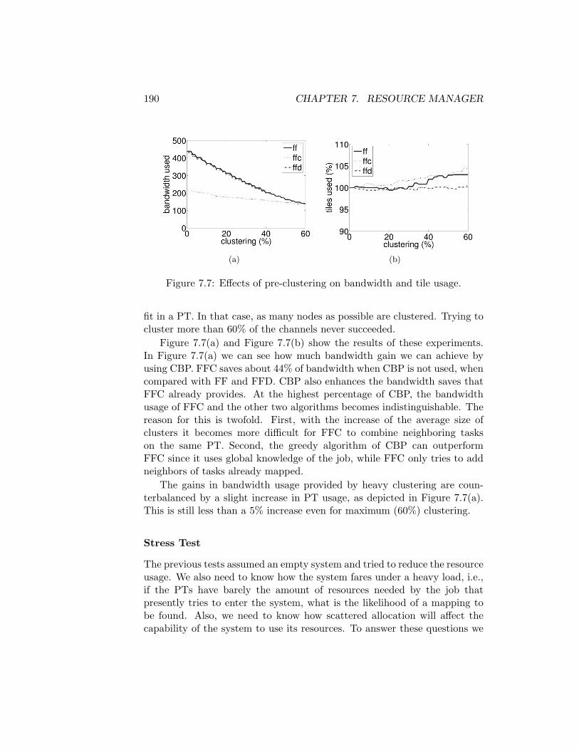
190 CHAPTER 7. RESOURCE MANAGER
(a) (b)
Figure 7.7: Effects of pre-clustering on bandwidth and tile usage.
fit in a PT. In that case, as many nodes as possible are clustered. Trying tocluster more than 60% of the channels never succeeded.
Figure 7.7(a) and Figure 7.7(b) show the results of these experiments.In Figure 7.7(a) we can see how much bandwidth gain we can achieve byusing CBP. FFC saves about 44% of bandwidth when CBP is not used, whencompared with FF and FFD. CBP also enhances the bandwidth saves thatFFC already provides. At the highest percentage of CBP, the bandwidthusage of FFC and the other two algorithms becomes indistinguishable. Thereason for this is twofold. First, with the increase of the average size ofclusters it becomes more difficult for FFC to combine neighboring taskson the same PT. Second, the greedy algorithm of CBP can outperformFFC since it uses global knowledge of the job, while FFC only tries to addneighbors of tasks already mapped.
The gains in bandwidth usage provided by heavy clustering are coun-terbalanced by a slight increase in PT usage, as depicted in Figure 7.7(a).This is still less than a 5% increase even for maximum (60%) clustering.
Stress Test
The previous tests assumed an empty system and tried to reduce the resourceusage. We also need to know how the system fares under a heavy load, i.e.,if the PTs have barely the amount of resources needed by the job thatpresently tries to enter the system, what is the likelihood of a mapping tobe found. Also, we need to know how scattered allocation will affect thecapability of the system to use its resources. To answer these questions we

7.5. EXPERIMENTS AND RESULTS 191
designed a stress test that constantly forces the allocator to map jobs underheavy load. This test works as follows.
First, we choose a job set J .For each job j ∈ J , the sum rj of the proces-sor cycles and memory requirements of its tasks and channels is calculated.Let t be the sum of all processor cycles and memory space still availablein the system. Vector t is updated whenever a job is started or stopped.The system starts without any jobs running. A job j which is not alreadyrunning, is selected at random, and is requested to start iff (1 + σ)rj ≤ t,where σ > 0 is an amount of slack. The slack parameter σ is introduced asit is very unlikely that any bin-packing algorithm (even an optimal one) iscapable of filling up the PTs to 100%. If the inequality (1 + σ)rj ≤ t doesnot hold , running jobs are stopped at random until the inequality does hold.The resource allocator is then requested to start the job.
The resource allocator receives this job start request and tries to mapthe job onto the unused resources. Its success or failure to do so is noted,and the next job is randomly selected. This is repeated for 10,000 iterationsfor several values of slack σ. During the first steps of the stress test theselected jobs will gradually fill up the system. After a while, the resourceallocator will be trying to map new jobs onto a heavily loaded system. Wecan then measure the number of successful mappings.
We have chosen several test job-sets. For each of these, we ran the stresstest for 10,000 iterations. The results shown are for the FFC algorithm,which provided the best results in the previous tests. The plot in Figure7.8(a) shows, for different percentages of CBP applied, the percentage ofsuccesses of the FFC algorithm plotted for different amounts of allowedslack. There are several things worth noting here. The first is that, if noCBP is used, less than 10% of slack is enough to virtually eliminate allmapping failures. The second is that CBP does not seem to work very well.A case analysis showed that the reason for this is that CBP creates clustersthat cannot be combined well on half-filled tiles, thus leaving large gapswhich the similarly large clusters of the new jobs cannot fill. In the previousexperiments, with an empty system, this problem could not be seen. Athird observation is that the graph occasionally spikes downwards with theincrease of slack. Case analysis showed this is due to the stress test gettingstuck in a local minimum, and a row of jobs fails to be mapped. This effect ismagnified at high CBP percentages, where fragmented mappings pose moreof a problem.
We decided to try to fix these problems by resorting to a fall-back mech-anism: if the RA cannot map the clustered version of the job, it tries to mapthe original, unclustered version. The results can be seen in Figure 7.8(b).

192 CHAPTER 7. RESOURCE MANAGER
(a) (b)
Figure 7.8: Mapping successes versus slack a) without fall-back and b) withfall-back.
With this modification, CBP does not affect negatively the performanceanymore and can even improve it slightly. Clustering optimizes bandwidthusage, not PT usage. To see if CBP is useful, the bandwidth requirementsof all jobs were scaled up and a slack of 10% was allowed. The results areshown in Figure 7.9. CBP does help in decreasing bus usage. With a factorof 3 increase in the bandwidth requirements, a clustering of 60% still allowsfor a success rate of 60%. Without any clustering, the success rate has gonedown to almost 0%.
Figure 7.9: Mapping successes with increased bandwidth requirements.

7.5. EXPERIMENTS AND RESULTS 193
Discussion of Results
For a 1-router system, the FF family of VBP algorithms provided a simpleyet effective base for an allocation heuristic. The best solution is a two-step approach: first, apply CBP and try FFC; second, if this fails, applyFFC with the original graph. This combined solution is capable of utilizingat least 95% of the available PT resources, if the bus bandwidth does notbecome a very scarce resource.
7.5.2 Systems with more than one router
For systems with more than one router, we tested several topologies, shownin Table 7.1. These topologies will be compared first. In a ring topology,routers are connected to neighboring routers in a one-dimensional grid. In amesh topology, routers are connected to north, south, east, west neighboringtasks in a two-dimensional grid.
Topology Size Links/router Tiles Routers Linksring-3 3 10 24 3 54ring-4 4 8 24 4 56ring-6 6 6 24 6 60ring-12 12 4 24 12 72mesh-6 2 by 3 6 22 6 58
Table 7.1: The topologies considered.
Effects of Topology
For each of the topologies of Table 7.1, the FFC algorithm was chosen to tryto map an instance of 100 tasks onto an empty system. We used the on-linevirtual placement method. This was tried for 100 instances, each mappedonto an empty system. The percentage of jobs that could successfully bemapped is shown against the clustering percentage in Figure 7.10.
We observe several facts from this figure. First, clustering is necessaryto be able to map any of the tested jobs onto any of the tested topologies.Secondly, the larger rings (ring-6 and ring-12) give bad performance (50%success rate or lower), while the performance for the other topologies issimilar (up to 70% success rate). This could be due to the fact that in ring-3, ring-4 and mesh-6, the average distance between two PTs is low. Hence,less congestion is likely to occur, which would hinder a successful mapping.What would be the optimal topology heavily depends on the cost function.

194 CHAPTER 7. RESOURCE MANAGER
0 20 40 600
20
40
60
80
100
clustering (%)su
cces
s (%
)
mesh−6ring−12ring−3ring−4ring−6
Figure 7.10: Successes per topology.
In our case, routers contain an all-to-all interconnection grid, thus havinga cost quadratic in the number of links they are connected to. Each linkand router also bears costs, further complicating judgment. For the rest ofthis chapter, we chose the ring-4 topology as a trade-off between number ofrouters and the number of links of each router, balancing the costs.
The rest of the tests will focus on the ring-4 topology.
Virtual Tile Placement
The best performance observed in all topologies was only a 70% success ratefor finding a mapping for a large job on an empty system. This percentageincreases if a different form of VT placement is used. In Figure 7.11, thesuccess rate is shown for the same job set on a ring-4 topology, using differentVT placement methods.
The difference between the on-line and semi on-line placement methodsis marginal. This can be explained by the little knowledge available andused by both algorithms when asked to place a VT. The on-line algorithmhas no knowledge of the contents of the tile, so has little information to per-form optimizations, other than choosing a location close to the tiles alreadymapped. The semi on-line algorithm knows which tasks are mapped to theVT it has to place, but does not know the location of all the tasks whichhave channels to it. As can be seen in Figure 7.11, this extra knowledgedoes not increase the performance significantly.
The off-line VT placement algorithm does prove to be a substantial im-provement over the on-line one. The success percentage is raised acrossall clustering percentages, reaching 90%. Even though the performance is

7.5. EXPERIMENTS AND RESULTS 195
0 20 40 600
20
40
60
80
100
clustering (%)
succ
ess
(%)
off−lineon−linesemi on−line
Figure 7.11: The percentage ofsuccessful mappings as a functionof the clustering percentage fordifferent placement algorithms.
0 20 40 6070
80
90
100
clustering (%)
links
use
d(%
)
off−lineon−linesemi on−line
Figure 7.12: The percentage oflinks used as a function of the clus-tering percentage, relative to theon-line algorithm.
better, clustering is still required to reach the higher chances of success.The difference in placement algorithms is not only visible in the per-
centage of successful mappings, but also in the number of links used bysuccessfully mapped jobs. The percentage of links used in the network, rel-ative to the number of links the basic on-line placement algorithm uses, isshown in Figure 7.12. The spikes at low clustering percentages occur be-cause there are relatively few successful mappings over which the averageis taken. Again, the on-line and semi on-line algorithm differ little in linkusage. The off-line algorithm attains a profit of 15% in the number of linksused, which is decent considering many routes that are optimized will be re-duced from length 3 (PT–router–router–PT) to length 2 (PT–router–PT),for which only a gain of 33% in length is possible. This directly impliesprofit in terms of power consumption and amount of free resources left forother jobs.
Using Shuffled Input
Another way to increase the chances of success is by trying to map severalrandom permutations on the ordering of the tasks to map. This results in afavorable increase as is shown in Figure 7.13. The figure shows the percent-age of successes when 1 to 4 random permutations are tried, increasing thesuccess rate up to over 95% when 4 permutations are tried.

196 CHAPTER 7. RESOURCE MANAGER
0 20 40 600
20
40
60
80
100
clustering (%)su
cces
s (%
)
1234
Figure 7.13: The percentage of successful mappings as a function of theclustering percentage. Each line represents a certain number of randomizedattempts.
Stress Test
The previous tests assumed an initially empty system. However, our solutionshould behave well under heavy load, i.e., if there are barely enough resourcesavailable in the system when there is a request to start a job.
We tested the performance under heavy load by taking the ring-4 topol-ogy and performing the stress test, as for the 1-router case.
The result of this test is shown for several clustering percentages inFigure 7.14. At σ = 0, there is no slack, implying the resource allocator hasto be capable of starting a job no matter how much the available resourcesare scattered. This is not always possible, so we cannot expect the resourceallocator to always succeed. As more slack is added, the resource allocatorhas more redundant free resources it can use, increasing the success ratedramatically. With only 5% slack, all requested jobs could be started if noclustering is used.
Another observation in relation to Figure 7.14 is that, as in the singlerouter case, clustering actually has a negative impact on performance. Thereason for this is that if clustering is applied, larger tasks are created thatrequire larger portions of free space on a PT. This requires the availableresources to be concentrated on fewer tiles, something that is less likelyto happen. Because clustering reduces bandwidth usage (and thus powerusage) as well as increases the feasibility of mapping bigger jobs, we did notwant to discard it. Instead, we use the same fall-back mechanism as in thesingle router case, in which first the job is clustered and an attempt is made
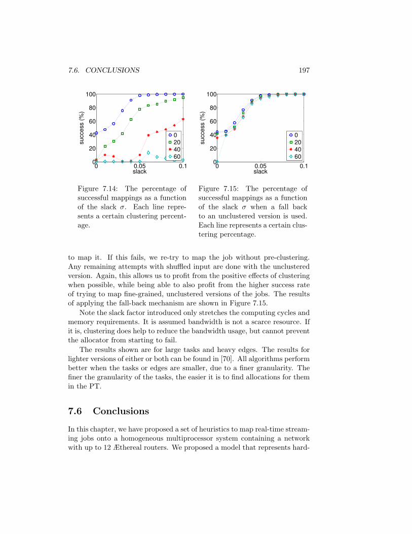
7.6. CONCLUSIONS 197
0 0.05 0.10
20
40
60
80
100
slack
succ
ess
(%)
0204060
Figure 7.14: The percentage ofsuccessful mappings as a functionof the slack σ. Each line repre-sents a certain clustering percent-age.
0 0.05 0.10
20
40
60
80
100
slack
succ
ess
(%)
0204060
Figure 7.15: The percentage ofsuccessful mappings as a functionof the slack σ when a fall backto an unclustered version is used.Each line represents a certain clus-tering percentage.
to map it. If this fails, we re-try to map the job without pre-clustering.Any remaining attempts with shuffled input are done with the unclusteredversion. Again, this allows us to profit from the positive effects of clusteringwhen possible, while being able to also profit from the higher success rateof trying to map fine-grained, unclustered versions of the jobs. The resultsof applying the fall-back mechanism are shown in Figure 7.15.
Note the slack factor introduced only stretches the computing cycles andmemory requirements. It is assumed bandwidth is not a scarce resource. Ifit is, clustering does help to reduce the bandwidth usage, but cannot preventthe allocator from starting to fail.
The results shown are for large tasks and heavy edges. The results forlighter versions of either or both can be found in [70]. All algorithms performbetter when the tasks or edges are smaller, due to a finer granularity. Thefiner the granularity of the tasks, the easier it is to find allocations for themin the PT.
7.6 Conclusions
In this chapter, we have proposed a set of heuristics to map real-time stream-ing jobs onto a homogeneous multiprocessor system containing a networkwith up to 12 Æthereal routers. We proposed a model that represents hard-

198 CHAPTER 7. RESOURCE MANAGER
ware constraints, and the resource requirements of jobs. Within this model,it is possible to reason about temporal guarantees, which allows us to mapjobs onto the system such that temporal constraints are met.
We showed how to model the Network-on-Chip in such a way that time-multiplexing can be taken into account by representing each router as anumber of communication nodes, one per time slice. The problem of findinga path through the network is then merged with the problem of finding avalid slot allocation table per router. The joint problem can be seen as adisjoint paths problem.
In order to map a job, its tasks and channels are packed onto the tilesusing a First-Fit strategy, after which routes through the network are allo-cated. We showed it is beneficial to use a two-step approach. First, we mapthe tasks onto virtual tiles (VTs), and then we map the VTs onto the ac-tual tiles. This raised the chance of finding a feasible mapping, and reducedbandwidth usage.
We also showed that chances of finding a feasible mapping can be furtherincreased by trying several random permutations on the ordering of theinput.
Our stress test shows how our resource manager performs under heavyloads. One interesting remark is that although clustering is essential to mapsome jobs, and greatly decreases bandwidth usage, it has an adverse effecton allocation success once the system is close to full. Because of this, wedevised a mechanism by which two versions of the job are tried out in themapping: first a clustered version, and, if this fails, an unclustered version.This allowed for a substantial increase in the percentage of successes duringthe stress test.
When operating under heavy load, the described approach seems to becapable of allocating 95% of the resources available on the processing tiles,assuming that bandwidth does not become a scarce resource.

Chapter 8
Demonstrator
The demonstrator prototype presented in this chapter was part of a largerdemonstrator built by Nokia, NXP and ST-Ericsson, where our basebandsoftware framework is integrated with the Radio Computer functional ar-chitecture proposed in [1]. It shows how the concepts we proposed can beworked out into an execution platform, even when the hardware was notdesigned to meet some of the requirements of our software framework. Italso shows how the custom components of our software framework can beimplemented while re-using a substantial amount of existing software.
As for the hardware, it uses an NXP prototype board for single-radio,integrating 2 EVPs, 3 ARMs, and hardware accelerators. All processorsrun at low clock frequencies: the EVPs at 183 MHz and the ARMs at61MHz. Each core has private data and instruction memories, and no cacheor memory management unit. Connectivity is provided by a tree of AXIbusses. Worst-case memory access latencies can be computed, since the AXIslave-side arbiters are Round-Robin. DMAs are not used, since bursts causelarge worst-case access times through the arbiters. The Resource Managerin this implementation supports at most 5 transceiver types and 5 jobs, anumber that was decided as a result of use-case analysis.
8.1 Streaming Framework: Sea-of-DSPs
In our demonstrator, Sea-of-DSPs (SoD) is a low-level multi-processor stream-ing OS that was developed initial at Philips and later at NXP Semicon-ductors. SoD was developed as a lightweight streaming framework for amulti-DSP chip.
SoD provides runtime support for the following features:
199
200 CHAPTER 8. DEMONSTRATOR
• Streaming Kernels: dynamic single-core schedulers on which taskscan be started and stopped; the default SoD scheduling policy is non-preemptive, round-robin;
• Streaming API: FIFO communication primitives;
• Network Manager API: can create, delete, resume and suspendtasks in any of the Streaming Kernels; and it can create or deleteFIFOs to connect tasks.
SoD is designed to function with minimal demands on memory footprintand cycle budget.
Internal memory management is done by reserving, at compile time,configurable memory pools for each object type. This results in predictablebehavior and no fragmentation. SoD has been ported to several processors:ARM, TriMedia, EVP (VD32040), EPICS7B, Tensilica Vectra LX DSP,HiFi 2. It can run in emulation mode on Windows and Linux. It has a lowmemory footprint: the Network Manager is less than 10 KByte of ARM7thumb code and the SoD SK (Streaming Kernel) code is less than 1 KByte.
The streaming API of SoD relies on shared memory access between com-municating cores. SoD allows FIFO buffers to be placed either at consumeror producer side. It also supports the usage of duplicated FIFO administra-tion at consumer and producer side, to avoid remote read operations.
An embedded hardware platform typically has its memory scatteredacross the system. Each core has local data and instruction memories, andshared system memories are also available. SoD offers several choices forthe location of the FIFO data and the FIFO administration. Dependent onthe latency of reads and writes to each of the memories, the most optimalpartitioning can be chosen when configuring SoD for a particular hardwareplatform. For example: in the case of a task on the ARM communicating toa task on an EVP, it is optimal to store the FIFO buffer and administrationin EVP local data memory. This because of the very high latency the EVPhas in writing to external/remote memories. In the case where two DSPshave to communicate, each DSP can read and write the local memories ofthe other DSP but remote reads will cause a much higher latency than thewrite cycles (posted writes). Thus the FIFO buffer is placed in the localmemory of the reading task.
SoD also minimizes latency/stall cycles caused by remote reads by em-ploying duplicated FIFO administration. If it is configured with that option,a copy of the FIFO administration table is placed at the local memory ofboth consumer core and producer core. Using this scheme, no remote reads

8.2. RESOURCE MANAGER IMPLEMENTATION 201
are required, since consumer and producer tasks simply check the state ofthe FIFO by reading their local copies. Of course than upon any change tothe administration of the FIFO requires both producer and consumer to up-date the local copy and the remote copy, but this only requires single-wordremote writes, which have a considerably lower latency than remote reads.
8.2 Resource Manager Implementation
The Base-band Resource Manager (BB-RM) uses the services provided bythe SoD Network Manager API. SoD already manages some resources. Itallocates memory for FIFO capacities, and creates tasks and FIFOs. It doesnot handle jobs as groups of interconnected tasks that must be admittedor rejected atomically. It merely finds and reserves resources for a singletask/channel at a time. It is not aware of timing requirements and doesnot perform scheduling tests. It does not chose task to processor mappings.BB-RM must take care of all these tasks.
BB-RM enforces strict admission control and resource reservation. Whenrequested by Central Resource Manager (see diagram in Figure 2.2 of Chap-ter 2) to start a transceiver, it performs admission check, trying to find afeasible processor assignment for all tasks of the transceiver.
As described in Chapter 7, the resource requirements of a transceiverare represented by a graph. Nodes represent the two types of resource con-suming entities: tasks (quasi-statically ordered clusters of MCDF actors)and channels (inter-cluster MCDF FIFOs). Each node has a requirementsvector. The vector fields are different from the model presented in Chap-ter 7, as the communication infrastructure does not contain communicationassists or a network-on-chip. For a task mapped to a TDM scheduler, thevector fields are: processor type, period, slice size, code memory read-writememory, and read-only memory. For NPNBRR schedulers, slice size is re-placed by worst-case execution time. Admission control checks if the sumof execution times/slices of tasks assigned to the core plus the executiontime/slice of the new task is lower than the deadlines of all tasks involved.For channels, the vector fields include buffer memory on the consumer andproducer side. The representation of resource requirements by a vector ofscalar fields is flexible and easy to port to different hardware platforms.
Processor assignment uses the adapted first-fit vector bin-packing algo-rithm described in Chapter 7 to fit the resource requirements of nodes tothe resource provision vectors of processors. The algorithm assumes thatmemory is not fragmented. After deriving a processor assignment, BB-RM

202 CHAPTER 8. DEMONSTRATOR
invokes a memory allocation procedure per segment. If memory allocationis successful, all tasks and FIFOs are instantiated. If instantiation succeeds,the transceiver is admitted. If not, BB-RM rolls back all reservations andinforms CRM of an in-feasibility. When CRM requests a job to stop, all itstasks are destroyed, and resources freed.
Since transceivers are compiled independently and processor assignmentis done at admission control, BB-RM supports dynamic loading with dy-namic linking to the Streaming API. The code in the transceiver configura-tion is compiled with relocation information that BB-RM uses to link andload the code at the addresses given by memory allocation.
BB-RM invokes a loader for each task. It provides it as input the startaddress and size of each allocated memory segment. The loader requests anobject file from the Configuration Manager for each task. This file is parsed,and the values for symbols left unresolved at compile time are now filled in.Code and read-only data are written into the memory of the processor towhich they were mapped. Symbols of newly loaded modules are added tothe internal symbol table of the framework so that they can be found bymodules loaded later.
8.3 Prototype Figures
In this section we evaluate the costs and overheads of our approach as evi-denced by the demonstrator.
8.3.1 Memory
The data memory of BB-RM dominates the footprint, requiring 49.8KB. Ofthis, 28.6 KB are spent in transceiver configuration. This requires two-fifthsof the memory of an ARM (128KB). However, there is plenty of room foroptimization. We set the number of components per transceiver to 50, to beable to store complete unclustered transceivers. This was needed for testing,but oversized: for the WLAN receiver, there are only 3 components afterclustering.
Memory allocation also consumes considerable space, at 13 KB. Thisis because of the fine granularity (32bits) at which blocks of memory areallocated. The SoD Network manager consumes a total of 25.6KB of datamemory, for its own configuration information. The Streaming Kernel re-quires 8.6 KB, both on EVP and ARM. For instruction memory, BB-RMrequires 24.5KB, and the Streaming Kernels require 1.6KB.

8.3. PROTOTYPE FIGURES 203
8.3.2 Performance of BB-RM
For a job containing 16 tasks and 22 FIFOs, the admission time is 201 ms,where 196 ms are taken by memory allocation. Processor allocation takesnegligible time (less than 5 ms). According to the specification, a new jobshould take less than one second to start, so these values are acceptable.If a need would arise for BB-RM to execute faster, the main area for op-timization is of course the memory allocation. As already mentioned, thecurrent granularity of memory allocation is in blocks of 1 word, using a Best-fit algorithm, that must scan all “holes” in the memory of a processor tofind the best allocation. This guarantees minimal memory fragmentation,but makes the process of memory allocation very slow. Memory allocationcould be made a lot faster by choosing a coarser granularity of memory blockallocation.
8.3.3 Scheduling Overhead
The scheduling overhead of the Streaming Kernel per task, for the EVP is99 ns at 183 MHz. When a task is activated, it checks for input data andoutput space. A check for data/space takes 135 ns, and an update of aFIFO management table takes 141 ns. The total synchronization overheadof a task that reads one FIFO and writes one FIFO is 135× 2 + 141× 2 +99 = 651ns. Table 8.1 depicts the synchronization overhead of one taskwith respect to the schedule period for relevant wireless standards ( sinceTDS-CDMAhas non-uniform symbol length, we took the duration of themidamble - the shortest symbol - as the schedule period).
The overhead is negligible for broadcast and connectivity standards. ForWLAN, an OFDM symbol arrives every 4 µs, and the overhead is 16.3% ofthe total schedule period. This overhead however, will decrease for higherprocessor clock frequencies, since the cycle count of the streaming kernelfunctions and the schedule period remain the same. It is also of note thatwe made a very straightforward port of the Streaming Kernel to the EVP,without using any EVP intrinsics, for instance, when dealing with compu-tation of memory addresses to access the circular FIFO buffers.
8.3.4 Multi-radio Operation
The prototype can only employ NPNBRR schedulers on the EVPs sinceits version of the core has no interrupt support. Consequently, only ra-dios working at about the same time granularity can share resources, e.g.2×DVB-T or 2×WLAN. The DF Scheduler computed resource budgets that

204 CHAPTER 8. DEMONSTRATOR
Standard Schedule Period Task Overhead (%)WLAN 802.11a 4µs 16.3%
LTE 71.4µs 0.32%TD-SCDMA 112.5µs 0.58%
UMTS 133µs 0.49%DVB-T/SH 935µs 0.07%
Table 8.1: Synchronization overhead per task.
accommodate these use cases using 2 ARM clusters and 1 EVP cluster. Inthe WLAN we scaled the execution times by 2, due to the low processorclock speeds on the prototype board. Using an interrupt-enabled EVP, aTDM scheduler with a 4µs period allows DVB-T and WLAN to run to-gether. This would cost a 13.7% context switching overhead, which is notinsignificant, but affordable for HRT multi-radio. The 2×WLAN use-casecan only be mapped with NPRR schedulers when clustering is applied. Infact, clustering is essential for demanding standards such as WLAN, dramat-ically reducing synchronization overhead. For WLAN, without clustering,each actor adds at least the 16.3% overhead shown in Table 8.1 to the totalresource expenditure, making mapping of two WLAN jobs sharing resourcesimpossible. With clustering, such overhead is only incurred once per clus-ter, and the mapping of two WLAN becomes possible. Table 8.1 also showsthat for standards other than WLAN the synchronization overhead is muchmore acceptable. Again, notice that these task synchronization overheadswere obtained by simply compiling the SoD API C code on EVP, with noplatform-specific optimizations, so there may still be plenty of room for op-timization.
8.3.5 Resource Fragmentation
We have not experienced resource fragmentation after multiple start/stoprequests. Our demonstrator supports few simultaneous transceivers and in-stances (4 of each). Since WLAN cannot share processors with slower radios,such as DVB-T or TD-SCDMA, due to the lack of preemptive schedulers inthe demonstrator, there is a natural limitation to the mappings: WLANs canonly be mapped to empty processors or to processors where other WLANsare already running. When a WLAN is stopped, it frees the exact spacethat a new WLAN instance will require.

8.4. CONCLUSION 205
8.4 Conclusion
The demonstrator shows how the concepts of our software framework can beput to practice, even on a platform that was originally designed as a demon-strator for single-radio operation. It also allows us to measure the memoryand performance overhead that each one of our run-time components addto a modem platform. For our implementation, these overheads turned outto still allow for two WLAN receivers to run simultaneously for a processorwith 2x the clock frequency of the EVPs in the prototype board – whichwere chosen to allow the execution of one single WLAN –, although with ahigh scheduling overhead of 16% of the WLAN period per task. Weighing inthe fact that WLAN is a standard with a much faster rate of operation thanmost other radio standards – in fact, for popular connectivity stadards thisoverhead is well bellow 1% of the cycle budget – and that the implemen-tation of the inter-task communication primitives was done by re-compilingoff-the-shelf C code, it is safe to state that the communication overhead ofa more realistic implementation for a less demanding standard should benegligeable.

206 CHAPTER 8. DEMONSTRATOR

Chapter 9
Conclusions and FurtherWork
We live in a planet overflown with information, where billions of wirelesslyconnected devices constantly send and receive data. Wireless connectivityis enabled through several different radio standards. Devices need to handlethis diversity, and, at times, must support several standards simultaneously.
The baseband layer of a wireless communication standard is often imple-mented on a heterogeneous multiprocessor platform. Each wireless standardhas its own strict temporal requirements. In systems that support a singlestandard at a time, the problem of mapping the application to the hardwarewith guaranteed temporal behavior is complex, but known to be manageablefrom an engineering perspective. This is typically done by doing schedulingmanually, or with little tool support and exhaustively verifying all possibleuse cases.
However, in an environment where multiple transceivers may be active si-multaneously, the problem becomes considerably more complex, as resourcecontention among transceivers may lead to unpredictable temporal behavior.
A solution to this problem is to assign fully separated resources to eachtransceiver. Such a solution is simple and clean, but neglects the fact thatsharing resources can lead to reduced costs in chip area, and cost is still amajor driving factor in high volumes electronics.
In this thesis we studied how to share hardware resources between trans-ceivers executing simultaneously, while still being capable of giving hardreal-time guarantees to each transceiver.
As a result, we proposed the first software framework that is capableof handling multi-radio execution with real-time guarantees, if used in con-
207
208 CHAPTER 9. CONCLUSIONS AND FURTHER WORK
junction with a predictable hardware platform. We proposed an automatedprogramming flow and a multiprocessor runtime for resource management,scheduling and inter-task communication. We have shown the feasibility ofsuch software framework, and we provided solutions for some main chal-lenges that we identified in building such a framework.
Our departing point was the observation that the main sources of unpre-dictable timing behavior are the functionality of the application itself andthe runtime resource management policies of the execution platform.
For the runtime, we proposed FIFO-based communication and synchro-nization, local budget schedulers per processor, and a global resource reser-vation mechanism, to effectively isolate the worst-case temporal behavior ofeach transceiver from the behavior of other running transceivers.
As a basis for a strict model of computation with strong analytical prop-erties and fitting expressivity, we picked data flow: its static variants havevery strong analytical properties, and since it is a concurrent, asynchronousmodel of computation, it lends itself well to distributed implementations.
We devised how the whole software framework and a runtime environ-ment based on these concepts should work. This was presented in Chapter2. The usage of a high-level language customized to describe data flow guar-antees correctness by construction and enables automatic model extractionand automatic code generation, which renders a more reliable tool chain,makes the source code more portable by allowing automatic generation ofplatform-specific API calls, and dramatically simplifies the job of the imple-menter.
We also identified a number of limitations of the state of the art re-garding the analytical properties of data flow, its expressivity, and mappingtechniques. We went on to figure out how some of these limitations couldbe overcome for wireless applications.
In Chapter 4, we studied latency and throughput analysis of data flow.Previous work on Multi-Rate Data Flow only allowed guarantees on a self-timed data flow execution for a minimum guaranteed throughput – averagedover a number of iterations dependent on the specific graph – and only afterthe graph had settled onto periodic behavior. We have shown that if theexternal source has a behavior that is upper-bounded by a periodic regime,we can guarantee a strictly periodic behavior for any actor in the graph,independently of any timing variations due to start-up behavior or variable(but bounded) execution times of other actors in the graph. We developedanalysis techniques that allow us to verify maximum bounds on latency– and therefore provide maximum latency guarantees - for the self-timedexecution of a multi-rate data flow graph, assuming either a periodic source,

209
a bursty source or a sporadic source.In Chapter 5, we proposed a scheduling strategy and an automated
scheduling flow that enable the simultaneous execution of multiple hard-real-time data flow jobs. Each job has its own execution rate and startsand stops independently from other jobs, at instants unknown at compile-time, on a multiprocessor system-on-chip. We have shown how such jobs, ifdescribed by a Multi-Rate Data Flow graph, can be automatically mappedonto a multi-processor system.
Our mapping strategy differentiates between intra-job scheduling andinter-job scheduling. Intra-job scheduling is handled at compile-time, throughthe generation of clusters of statically-ordered actors, and the computationof buffer sizes for arcs between actors. Inter-job scheduling is solved at run-time by using schedulers such as either Time-Division Multiplex (TDM)or Non-Preemptive Non-Blocking Round Robin (NPNBRR), depending onwhether the processor supports preemption or not. At compile time, wecompute settings for the runtime schedulers per job.
We showed how a combination of TDM or NPNBRR and static-orderscheduling can be modeled as additional nodes and edges on top of thedata flow representation of the job using Single-Rate Data flow semantics,to enable tight worst-case temporal analysis. Based on this analysis model,we proposed algorithms to find combined TDM/NPNBRR and static orderschedules for jobs that guarantee a requested minimum throughput andmaximum latency, while minimizing the usage of processing resources. Weillustrated the usage of these techniques for a combination of Wireless LANand TDS-CDMA radio jobs running on a prototype Software-Defined Radioplatform.
One of the main limitations of data flow for our application domain isthat radios do have some data dependent behavior which cannot be rep-resented by the static variants of data flow (single-rate, multi-rate andcyclo-static) that allow temporal analysis. Because of this, we proposedin Chapter 6 an extension of static data flow that allows a limited amountof data dependent behavior, while preserving most of the temporal prop-erties. We named it Mode-Controlled Data Flow (MCDF). We proposedtiming analysis techniques that allow us to reason both in terms of mini-mum sustainable throughput and maximum latency for MCDF graphs, andmapping techniques that allows us to compute budgets for MCDF graphs,by extending the techniques we proposed for MRDF graphs. We also showedhow a WLAN 11a receiver can be modeled in MCDF, and mapped onto avirtual platform.
Given the budgets computed by our compile-time tools, we need to al-

210 CHAPTER 9. CONCLUSIONS AND FURTHER WORK
locate and reserve resources across the multiprocessor to meet the budgetrequirements of a transceiver, whenever the transceiver is required to exe-cute. In Chapter 7, we proposed algorithms to solve this runtime mappingproblem, including allocation of network resources in hardware architectureswhere a Network-On-Chip is used for inter-processor communication.
To bring all components of our solution together, we implemented ourmapping tools and our runtime software to target a prototype chip for base-band processing. This experiment, described in Chapter 8, allowed us toshow that our intended software framework could be built from a combi-nation of standard runtime OSes, existing compilation tools, and our owncustom software, in a modular manner. We showed that our run-time couldrun on a pre-existing hardware platform, and that the temporal runtimeoverhead that our scheduling policies required was acceptable from the per-spective of the application requirements, even for an unoptimized, prototypeimplementation such as ours.
In summary, we have shown that an approach based on resource bud-geting combined with a strict data flow computation model can very well bethe way to go for developing multi-radio systems.
Nonetheless, the list of topics that require future work is a long one. Torefer only some of the most important ones:
• (Quasi)-Static-order scheduling and clustering algorithms: our algo-rithm for static ordering has exponential complexity, and can, forlarger graphs, take a long time to terminate. Its adaptation to han-dle quasi-static ordering for MCDF suffers from even larger executiontimes, due to the fact that many different static orders correspond tothe same quasi-static order (this is attenuated somehow by our usageof state hashing). The development of heuristics for static-orderingand quasi-static ordering, potentially combined with other steps ofthe mapping flow such as scheduler settings determination and buffersizing minimization is certainly useful, and very likely necessary, iflarger graphs are to be handled.
• MCDF Extensions: Mode-Controlled Data Flow, as presented in thisthesis, is single-rate; although some limited forms of multi-rate behav-ior should be reasonably easy to handle with the existing techniques,it would be interesting to study what gains in expressivity could comefrom allowing, for instances, multi-rate behavior for the variable-rateactors. Also, the imposition of having a single mode controller makestemporal analysis much simpler, but makes it very cumbersome to

211
express applications with a very complex control structure. This sug-gests that further work is needed in supporting MCDF graphs withmultiple mode controllers, including the special case of hierarchicalcontrol.
• MCDF buffer sizing: in our work, we only provide crude upper boundsto the amount of buffer sizing necessary for meeting the timing require-ments for a given MCDF graph, using pre-defined reference static-order schedules. There is work to do on optimizing buffer sizing algo-rithms. A promising lead here is the work on buffer sizing for Variable-Phased Data Flow (VPDF). Since VPDF seems to be a superset ofMCDF, VPDF buffer sizing algorithms should be simple to adapt forMCDF.
• Budget Schedulers: in our work, we used only NPNBRR and TDMschedulers. TDM, however, provides rather poor trade-offs betweenresponse latency and throughput – for instance, if one wants a lowlatency for a task, one may need to allocate many more TDM resourcesthan required by the load of the task, just to reduce arbitration time.Other schedulers, such as the Priority-based Budget Scheduler [83]or the Credit-Controlled Static Priority arbiter [2] allow for betterresource usage. There is nothing in our flow that cannot be adaptedto work with other schedulers, as long as a conservative data flowmodel can be provided for the temporal behavior of a static-order ofsingle-rate data flow actors running on such a scheduler – which is thecase for both PBS and CCSP.
• Resource Fragmentation: In our work on resource management, weassumed that memory did not fragment. The reason for this is thatwe assumed a resource defragmentation technique would be available,as there was some active research on the topic at the time. To thebest of our knowledge, the problem is still largely unsolved.
• Power-aware scheduling was probably the most important aspect thatwe neglected in our work. Our work concerned itself with trying tooptimize mappings for reduced resource usage. However, for portabledevices, which are powered by a small battery and cannot use the samesort of cooling technology found in more sedentary devices, power andenergy consumption are very important, even primary, concerns. Ourwork, as most of the work in data flow analysis and scheduling per-formed in the past, did not address these concerns. It is relatively

212 CHAPTER 9. CONCLUSIONS AND FURTHER WORK
easy to conjecture on how our techniques could be extended to ad-dress power and energy minimization, since we can easily model therelations between resource utilization and temporal behavior, and tem-poral analysis can probably be done in the same way, but finding map-ping and resource management algorithms that try to optimize powerand energy consumption is still to be done.
All of the listed problems are of research interest, and the solutionsthat we will find for them will certainly impact the adoption of data flowtechniques by modem developers. It is our opinion that very satisfactorysolutions can be found for most, if not all of them.
However, the adoption by the industry of many of the concepts we use inour work is challenged by other factors that are more difficult to overcome.
To start, there are the customary difficulties related with the adoptionof a new technology. Most companies in the industry have mature designprocesses in place, and staffs of extremely gifted, experienced and knowl-edgeable engineers. A change to a platform design strategy centered onbudget based resource allocation and data flow based programming may bea step too far, as it requires new skills, new processes and new tools. Evenif the current industry approach cannot really handle multi-radio require-ments, it is likely that small incremental changes to the current approach,however complex or inefficient, will be preferred instead of a departure to-wards a completely new mind set. So a challenge for us is finding a paththrough small steps in the direction of our proposed solution.
This brings us to another issue: the technology is not yet mature. Notonly there are still many problems to address, but, for the time being, wecannot offer mature tooling support for data flow-based modem design.Tools such as the ones we developed during the course of our work, andsimilar ones, are not ready for the prime time. They have been designedprimarily as research vehicles by small teams of researchers, not as industrial-strength CAD tools.
Even more challenging may be the fact that the complexity and evenfeasibility of data flow modeling of hardware architecture constraints is verydependent on the platform. For instances, fixed priority arbiters and sched-ulers are difficult to model satisfactorily, but they are very common in exist-ing platforms. Even if it is often true that many such architectural choicesprevent the system from being predictable, and should therefore not be usedin designing a hard-real time system, it is also often true that although agiven scheduler or arbiter has no bounded worst case in general, a boundcan still be provided under certain reasonable assumptions. A good example
213
of this is again a fixed-priority scheduler – once we have a best-case charac-terization of the activation pattern and resource usage of all higher prioritytasks, we can easily provide a tight characterization of the temporal behav-ior of any given task. This breaks the basic principles of our approach, as itrequires knowledge of the temporal behavior of one or more jobs (includingtheir best case behavior) in order to characterize the worst case behaviorof another, and it does not preserve temporal monotonicity, becoming assuch vulnerable to scheduling anomalies. However, in practice, it may workfor many specific cases. It is certainly likely that during the design processor even later, when the product is already delivered, it will fail due to, forinstance, a last minute change in the behavior of a high priority task thatwas not accounted for in the temporal analysis of other tasks.
Nonetheless, the fact remains that some form of analysis is possible, inideal conditions, without the usage of our techniques, and this makes itdifficult to argue a priori that the system is not going to be predictableand that it must be completely changed to accommodate for a data flow-driven design, leaving the data flow advocate often in the role of a “prophetof doom”, constantly warning developers against catastrophes that may ormay not occur.
Thus the bottom line is that data flow based techniques must be intro-duced to the industry gradually. In fact, this is one of the reasons we stroveto have a modular software framework in Chapter 2. Each component ofthe framework was designed such that it is useful by itself, even if the othercomponents are missing. For instances, our resource manager can be com-bined with manual generation of budgets. Our data flow analysis tools canbe used to analyze a data flow model that was manually extracted from theapplication description. A data flow input language, combined with a goodcode generator, can provide a lot of advantages to the programmer by allow-ing code that is platform independent to be generated, and give guaranteesthat platform-specific APIs are correctly used. “Selling” the approach inbits is one way to build an incremental path to adoption.
More important than anything is to understand the application, therequirements and the platform; understand that real-time behavior is oneamongst many concerns of the design team, accept that sometimes we willhave to do with non-enforceable assumptions and try to make the analysiswork with as few changes as possible to the platform and design process.
In any case, and however difficult the introduction of data flow may be,it may soon become absolutely necessary to find a new way of designingmodems. The techniques that are currently used cannot scale with theincreased complexity of the transceivers, and the increase in the number of

214 CHAPTER 9. CONCLUSIONS AND FURTHER WORK
transceiver combinations that must be supported. We believe our approachfinds a good compromise between simplicity, performance and robustness,while meeting the requirements, but it still needs the maturity that onlyyears of actual product development can bring.

Bibliography
[1] A. Ahtiainen et al. Multiradio scheduling and resource sharing on asoftware defined radio computing platform. In Proc. Software-DefinedRadio Forum Technical Conference, Oct. 2008.
[2] B. Akesson, L. Steffens, E. Strooisma, and K. Goossens. Real-timescheduling using credit-controlled static-priority arbitration. In Pro-ceedings of the 2008 14th IEEE International Conference on Embed-ded and Real-Time Computing Systems and Applications, pages 3–14,Washington, DC, USA, 2008. IEEE Computer Society.
[3] F. Baccelli, G. Cohen, G. Olsder, and J.-P. Quadrat. Synchronizationand Linearity. John Wiley & Sons, Inc., 1992.
[4] S. K. Baruah and S. Funk. Task assignment in heterogenous multi-processor platforms. Technical report, University of North Carolina,2003.
[5] J. Beck and D. Siewiorek. Modeling multicomputer task allocationas a vector packing problem. In Proceedings of the 9th internationalsymposium on System synthesis, ISSS ’96, pages 115–, Washington,DC, USA, 1996. IEEE Computer Society.
[6] M. Bekooij et al. Predictable embedded multiprocessor system design.In Proc. Int’l Workshop SCOPES, LNCS 3199. Springer, Sept. 2004.
[7] M. Bekooij et al. Dataflow analysis for real-time embedded multipro-cessor system design. In Dynamic and Robust Streaming in and be-tween Connected Consumer Electronic Devices, volume 3, pages 81–108.Springer, 2005.
[8] K. Berkel et al. Vector processing as an enabler for software-definedradio in handheld devices. EURASIP Journal on Applied Signal Pro-cessing, 2005(16), 2005.
215

216 BIBLIOGRAPHY
[9] G. Bilsen et al. Cyclo-static dataflow. IEEE Transactions on SignalProcessing, 44(2):397–408, 1996.
[10] J. Buck. Scheduling dynamic dataflow graphs with bounded memoryusing the token flow model. PhD thesis, Univ. of California, Berkeley,September 1993.
[11] J. Buck. Static scheduling and code generation from dynamic dataflowgraphs with integer-valued control streams. In Proc. of the AsilomarConference on Signals, Systems, and Computers, 1994.
[12] G. Buttazzo. Hard Real-Time Computing Systems. Kluwer AcademicPublishers, 1997.
[13] J. Cochet-Terrasson et al. Numerical computation of spectral elementsin max-plus algebra. In Proc. IFAC Conf. on Syst. Structure and Con-trol, 1998.
[14] E. G. Coffman, Jr., E. G. Coffman, D. S. Johnson, D. S. Johnson, L. A.Mcgeoch, L. A. Mcgeoch, R. R. Weber, and R. R. Weber. Bin packingwith discrete item sizes part ii: Average-case behavior of ffd and bfd.In preparation, 13:384–402, 1997.
[15] T. Corman et al. Introduction to Algorithms. McGraw-Hill, 2001.
[16] D. Culler et al. Parallel Computer Architecture: a hardware/softwareapproach. Morgan Kaufmann, 1999.
[17] A. Dasdan. Experimental analysis of the fastest optimum cycle ratioand mean algorithms. ACM Transactions on Design Automation ofElectronic Systems, 9(4):385–418, Oct. 2004.
[18] E. W. Dijkstra. Hierarchical ordering of sequential processes. ActaInformatica, pages 115–138, 1971.
[19] D. Feitelson. Job scheduling in multiprogrammed parallel systems.Technical report, IBM Research Report RC, 1994.
[20] G. Gao, R. Govindarajan, and P. Panangaden. Well-behaved dataflowprograms for DSP computation. In International Conference of Acous-tics, Speech and Signal processing, 1992.
[21] M. R. Garey and D. S. Johnson. Computers and Intractability; A Guideto the Theory of NP-Completeness. W. H. Freeman & Co., New York,NY, USA, 1990.

BIBLIOGRAPHY 217
[22] M. Geilen. Dataflow scenarios. In IEEE Transactions on Computers,2010.
[23] M. Geilen and S. Stuijk. Worst-case performance analysis of syn-chronous dataflow scenarios. In ACM CODES + ISSS, 2010.
[24] A. Ghamarian, M. Geilen, S. Stuijk, T. Basten, A. Moonen, M. Bekooij,B. Theelen, and M. Mousavi. Throughput analysis of synchronous dataflow graphs. In Proc. Int’l Conf. on Application of Concurrency toSystem Design (ACSD), pages 25–34, June 2006.
[25] A. H. Ghamarian, S. Stuijk, T. Basten, M. Geilen, and B. D. Theelen.Latency minimization for synchronous data flow graphs. In DSD, pages189–196, 2007.
[26] A. Girault, B. Lee, and E. Lee. Hierarchical finite state machines withmultiple concurrency models. IEEE Trans. on Computer-Aided Designof Integrated Circuits and Systems, 18(6):742–760, June 1999.
[27] GNU Project. GLPK website. In http://www.gnu.org/software/glpk/,2011.
[28] S. Goddard and K. Jeffay. Managing latency and buffer requirementsin processing graph chains. The Computer Journal, 44(6), 2001.
[29] K. Goossens, J. Dielissen, J. van Meerbergen, P. Poplavko,A. Radulescu, E. Rijpkema, E. Waterlander, and P. Wielage. Guaran-teeing the quality of services in networks on chip, pages 61–82. KluwerAcademic Publishers, Hingham, MA, USA, 2003.
[30] K. Goossens, P. Wielage, A. Peeters, and J. Van Meerbergen. Networkson silicon: Combining best-effort and guaranteed services. In Proceed-ings of the conference on Design, automation and test in Europe, DATE’02, pages 423–, Washington, DC, USA, 2002. IEEE Computer Society.
[31] K. Goossens et al. Guaranteeing the quality of service in networks onchip. Kluwer, 2003.
[32] R. Govindarajan, G. Gao, and P. Desai. Minimizing memory require-ments in rate-optimal schedules. In Proc. Int’l Conf. on Application-Specific Array Processors, pages 75–86, Aug. 1993.
[33] R. Govindarajan and G. G.R. A novel framework for multirate schedul-ing. In International Conference on Application Specific Array Proces-sors, 1993.

218 BIBLIOGRAPHY
[34] M. Grant and S. Boyd. CVX: Matlab software for disciplined convexprogramming, version 1.21. http://cvxr.com/cvx, Feb. 2011.
[35] M. Grant, S. Boyd, and Y. Ye. Disciplined convex programming. InGlobal Optimization: From Theory to Implementation, Nonconvex Op-timization and Its Application Series, pages 155–210. Springer, 2006.
[36] C. Grassmann, M. Richter, and M. Sauermann. Mapping the physi-cal layer of radio standards to multiprocessor architectures. In Proc.Design, Automation and Test in Europe Conference and Exhibition(DATE), pages 1412–1417, 2007.
[37] W. Gropp et al. Using MPI: Portable Parallel Programming with theMessage Passing Interface. MIT Press, 1994.
[38] S. Ha and E. Lee. Compile-time scheduling of dynamic constructsin dataflow program graphs. IEEE Transactions on Computers,46(7):768–778, July 1997.
[39] A. Hansson. A Composable and Predictable On-Chip Interconnect. PhDthesis, Eindhoven University of Technology, 2009.
[40] A. Hansson, K. Goossens, and A. Radulescu. A unified approach toconstraint mapping and routing on network-on-chip architectures. InInt’l Symposium on System Synthesis (ISSS), pages 75–80, 2005.
[41] A. Hansson, K. Gossens, M. Bekooij, and J. Huisken. Compsoc: A tem-plate for composable and predictable multi-processor system on chips.ACM Transactions on Design Automation of Electronic Systems, Oct.2009.
[42] B. Hayes. Cloud computing. ACM Communications of the ACM,51(7):9–11, July 2008.
[43] W. Heisenberg. The Physical Principles of Quantum Theory. Universityof Chicago Press, 1930.
[44] T. A. Henzinger. Two challenges in embedded systems design: pre-dictability and robustness. Philosophical Transactions of the Royal So-ciety, Oct. 2008.
[45] International Telecommunications Union. Measuring the InformationSociety 2010 - The ICT Development Index. http://www.itu.int, Dec.2010.
BIBLIOGRAPHY 219
[46] M. Jersak, K. Richter, and R. Ernst. Performance analysis of complexembedded systems. International Journal of Embedded Systems, 1(1-2):33–49, 2005.
[47] Joint Tactical Radio Systems Program Office. Software communicatonsarchitecture specification. http://sca.jpeojtrs.mil/.
[48] Joyent. What is cloud computing? www.youtube.com, 2008.6PNuQHUiV3Q.
[49] G. Kahn. The semantics of a simple language for parallel programming.In Proceedings IFIP Congress, pages 471–475, 1974.
[50] B. Kernighan and S. Lin. An efficient heuristic procedure for partition-ing graphs. The Bell System Technical Journal, 1970.
[51] S. G. Kolliopoulos and C. Stein. Approximating disjoint-path prob-lems using greedy algorithms and packing integer programs. In Lec-ture Notes in Computer Science, volume 1412/1998, pages 153–168.Springer-Verlag, 1998.
[52] Kopetz. Real-Time Systems: Design Principles for Distributed Embed-ded Applications. Springer, 1997.
[53] B. Korte and J. Vygen. Combinatorial Optimization: Theory and Al-gorithms. Springer-Verlag Berlin Heidelberg, 2002.
[54] L. Kou and G. Markowski. Multidimensional bin packing algortihms.IBM Journal of Research and Development, 22(2), 1977.
[55] P. Kourzanov. http://bitbucket.org/pjotr/lime/src/tip/doc/.
[56] E. Lee. The problem with threads. IEEE Computer, pages 60–67, 2006.
[57] E. Lee and D. Messerschmitt. Static scheduling of synchronous dataflow programs for digital signal processing. In IEEE Transactions onComputers, 1987.
[58] E. Lee and D. Messerschmitt. Synchronous data flow. In Proceedingsof the IEEE, 1987.
[59] J. Liebeherr, A. Burchard, Y. Oh, and S. H. Son. New strategies forassigning real-time tasks to multiprocessor systems. IEEE Trans. Com-put., 44:1429–1442, December 1995.

220 BIBLIOGRAPHY
[60] Y. Lin, Y. L. Hyunseok, M. Woh, Y. Harel, S. Mahlke, T. Mudge, andC. Chakrabarti. Soda: A low-power architecture for software radio.In In Proc. of the 33rd Annual International Symposium on ComputerArchitecture, pages 89–101, 2006.
[61] Y. Lin et al. Spex: A programming language for software defined ra-dio. In Proc. Software-Defined Radio Forum Technical Conference, Oct.2006.
[62] Y. Lin et al. Hierarchical coarse-grained stream compilation for softwaredefined radio. In Proc. Int’l Conf. on Compilers, Architectures andSynthesis for Embedded Systems (CASES), October 2007.
[63] C. L. Liu and J. W. Layland. Scheduling algorithms for multiprogram-ming in a hard-real-time environment. J. ACM, 20:46–61, January1973.
[64] T. Lundqvist and P. Stenstrom. Timing anomalies in dynamicallyscheduled microprocessors. In Proc. Real-Time Systems Symposium,1999.
[65] F. Malerba, R. Nelson, L. Orsenigo, S. Winter, F. Malerba, R. Nelson,L. Orsenigo, and S. Winter. A history-friendly model of the co-evolutionof the computer and semiconductors industries: Capabilities and tech-nical change as determinants of the vertical scope of firms in relatedindustries, 2006.
[66] T. Marescaux, B. Bricke, P. Debacker, V. Nollet, and H. Corporaal.Dynamic time-slot allocation for qos enabled networks on chip. In ES-TImedia, pages 47–52, 2005.
[67] G. Martin and H. Chang. Winning the SoC Revolution. Kluwer Aca-demic Publishers, 2003.
[68] J. Mitola. The software radio. In Proc. IEEE National TelesystemsConference. IEEE Computer Society Press, 1992.
[69] T. Miyazaki and E. Lee. Code generation by using integer-controlleddata flow graph. In Proc. ICASSP, 1997.
[70] J. Mol. Resource allocation for streaming applications in multiproces-sors. Technical report, Delft University of Technology, 2004.

BIBLIOGRAPHY 221
[71] A. Moonen, M. Bekooij, and J. van Meerbergen. Timing analysis modelfor network based multiprocessor systems. In Proc. Workshop of Cir-cuits, System and Signal Processing (ProRISC), pages 91–99, Veld-hoven, The Netherlands, 2004.
[72] O. Moreira, T. Basten, M. Geilen, and S. Stuijk. Buffer sizing forrate-optimal single-rate data-flow revisited. In IEEE Transactions onComputers, 2010.
[73] O. Moreira and M. Bekooij. Self-timed scheduling analysis for real-time applications. EURASIP Journal on Advances in Signal Processing,2007.
[74] O. Moreira, M. Bekooij, and J. Mol. Online resource management for amultiprocessor with a network-on-chip. In Proc. ACM Symposium onApplied Computing, March 2007.
[75] O. Moreira, M. Bekooij, J. Mol, and J. van Meerbergen. Multiproces-sor resource allocation for hard real-time streaming with a dynamic jobmix. In Proc. IEEE Real-Time and Embedded Technology and Applica-tions Symposium (RTAS), March 2005.
[76] O. Moreira, F. Valente, and M. Bekooij. Scheduling multiple indepen-dent hard-real-time jobs on a heterogeneous multiprocessor. In Proc.Embedded Software Conference (EMSOFT), October 2007.
[77] Q. Ning and G. Gao. A novel framework of register allocation for soft-ware pipelining. In Proceedings of the ACM SIGPLAN-SIGACT Sym-posium on Principles of Programming Languages, pages 29–42, 1993.
[78] T. M. Parks. Bounded Scheduling of Process Networks. PhD thesis,Princeton University, 1987.
[79] P. Poplavko, T. Basten, M. Bekooij, J. van Meerbergen, and B. Mes-man. Task-level timing models for guaranteed performance in multi-processor networks-on-chip. In Proc. Int’l Conf. on Compilers, Archi-tectures and Synthesis for Embedded Systems (CASES), pages 63–72,2003.
[80] U. Ramacher. Software-defined radio prospects for multi-standard mo-bile phones. IEEE Computer, 2007.
[81] R. Reiter. Scheduling parallel computations. Journal of the ACM,15(4):590–599, October 1968.

222 BIBLIOGRAPHY
[82] S. Sriram and S. Bhattacharyya. Embedded Multiprocessors: Schedulingand Synchronization. Marcel Dekker Inc., 2000.
[83] M. Steine, M. Bekooij, and M. Wiggers. A priority-based budget sched-uler with conservative dataflow model. In DSD, pages 37–44, 2009.
[84] D. Stiliadis and A. Varma. Latency-rate servers: a general model foranalysis of traffic scheduling algorithms. IEEE/ACM Trans. Netw.,6(5):611–624, 1998.
[85] M. Strik et al. Heterogeneous multiprocessor for the management ofreal-time video and graphics streams. IEEE Journal of Solid-State Cir-cuits, 35(11):1722–1731, 2000.
[86] S. Stuijk, M. Geilen, and T. Basten. Throughput-buffering trade-offexploration for cyclo-static and synchronous dataflow graphs. In IEEETransactions on Computers, 2008.
[87] S. Stuijk, M. Geilen, and T. Basten. A predictable multi-processordesign flow for streaming applications with dynamic behavior. In DSD,2010.
[88] S. Stuijk et al. Multiprocessor resource allocation for throughput-constrained synchronous dataflow graphs. In Proc. Design AutomationConference (DAC), 2007.
[89] B. Theelen et al. Scenario-aware data flow model for combined long-runaverage and worst-case performance analysis. Int’l Conf MEMOCODE,2006.
[90] W. Thies. Language and Compiler Support for Stream Programs. PhDthesis, Massachusetts Institute of Technology, 2009.
[91] D. tzen Peng, K. G. Shin, and T. F. Abdelzaher. Assignment andscheduling communicating periodic tasks in distributed real-time sys-tems. IEEE Transactions on Software Engineering, 23:745–758, 1997.
[92] M. Wiggers. Aperiodic Multiprocessor Scheduling. PhD thesis, Univer-sity of Twente, June 2009.
[93] M. Wiggers, M. Bekooij, M. Geilen, and T. Basten. Simultaneous bud-get and buffer size computation for throughput-constrained task graphs.In Proceedings of the Design, Automation and Test in Europe (DATE)Conference, 2010.

BIBLIOGRAPHY 223
[94] M. Woh et al. From soda to scotch: The evolution of a wireless base-band processor. In ACM International Symposium on Microarchitec-ture, 2008.
[95] O. Zapata and P. Mejia-Alvarez. Analysis of real-time multiproces-sors scheduling algorithms. In Proceedings of the Real-Time SystemsSymposium (RTSS), 2003.

224 BIBLIOGRAPHY

Acknowledgements
Through the process of moving to a different country and working on indus-trial research for eleven years and three companies, I have met many peoplewho taught me, inspired me, or influenced my thinking in ways that wereeventually reflected in the contents of this thesis. I am immensely gratefulto all of them. However, since it is unfeasible to mention everybody, I willtry to at least name the ones who had a direct impact on the work presentedhere.
First, I want to mention Bernardo Kastrup, because he was at the startof all of this. He created the opportunity for me to come to the Netherlandsand he introduced me to the large community involved in embedded systemsresearch in the Eindhoven area. It was with his guidance that I took my firststeps in research. He is very creative, charismatic, and enthusiastic abouthis many projects and ideas. Conversations with him never get boring. Iam proud to count him among my friends.
I wish to thank all the guys at the Compiler Technology cluster of PhilipsResearch circa 2000. Those were important formative years, when my un-derstanding of the virtues of formalism and design flow automation came tobe. The CT cluster was an exciting environment, where challenging tech-nical work was mixed with chess games, dinners in good restaurants, andintrincate philosophical arguments that went on until it was closing time atthe cafe Berlage.
I wish to thank Prof. Jef van Meerbergen for accepting me as a PhD can-didate, and helping me go through the process of admission and certificationat the TUE. His quiet demeanor can fool you into not realizing how sharpand incisive his thought is, or how wide and clear his vision of technology.Sadly, due to personal reasons, he could not supervise this work to its end.
Leszek Holenderski is a brilliant and uncompromising scientist. I learntfrom him not to confuse syntax with semantics. Our neverending argumentsprovided me with plenty of training in dialectic. Moreover, he introducedme to the Ocaml language, which made the implementation of my tools less
225

of a chore and much more of a pleasure.I am not well-versed in the actual workings of radio baseband applica-
tions, and it would have been impossible for me to model their behaviorand understand the temporal requirements without the help of experts. Mythanks to Ozgun Paker and Rick Nas for helping me with it. I owe the initialWLAN model that was the source of so many ideas to them.
Building the prototype tool chain and runtime described in this thesisis much more work than a single man can handle, so here goes a big thankyou to the guys from NXP and ST-Ericsson that worked on the demon-strator. Petr Kourzanov was the main designer of LIME and implementedthe parser and code generator for it, while elucidating me on the differencesbetween Western and Russian concepts of heroism; Marinus van Splunterwas our know-it-all specialist in streaming frameworks; Artur Burchard im-plemented the memory allocator, and David van Kampen was everywhere,fixing stuff whenever fixing was needed, and programming the “glue” thatwould hold the whole demonstrator together. My thanks also to Erik Lam-bers, who, as the group leader responsible for the Software-Defined Radioproject at NXP Semiconductors, believed in my ability to make the demon-strator happen. Thanks also to our research partners in the Nokia ResearchCenter in Helsinki, from whom I learnt about modem requirements andsoftware engineering practices.
I supervised the work of many master students during these 9 years.Working with each different personality was one of the most enriching expe-riences of my professional life, so thanks to all of you. Directly relevant tothis thesis was the work of five of them. Jan David Mol co-designed with methe online resource allocation algorithms, and carried out the implementa-tion and experimental evaluation. Frederico Valente cleaned up the mess Imade in the data flow scheduler. He also programmed and tested the slicingalgorithms and the data flow simulator. He was the student that managedto puzzle me by not asking questions, not having doubts, and still managingto get things done correctly. Emanuel Miranda implemented the versionof the resource manager that made it to the demonstrator, and along theway fixed many practical issues that we ignored when designing the originalalgorithms. Pedro Pereira implemented the buffer sizing algorithms basedon linear programming. Feiteng Yang implemented parts of the MCDFanalysis.
I would like to thank the management of ST-Ericsson, and Herman Ravein particular, for allowing me to take time to work on this, and making thefinalization of the manuscript one of my professional targets for the year2011. Without that extra push, I don’t know if I would have made it to the

end line.Prof. Henk Corporaal became involved in my thesis work relatively late,
but I cannot overstate how pleasurable it was working with him. His helpwith structuring the text and fleshing out the contents was invaluable, aswere his rigor, inquisitive attitude, and great sense of humor.
I also have a debt of gratitude to Marc Geilen. He only became involvedin my work at a late stage, but his thorough revision of the manuscriptspotted many problems. He is a truly remarkable expert in data flow, andhis eye for detail is second to none. I wish I had been able to cooperate withhim at an earlier stage. I would have wasted less time backtracking on mymistakes.
Marco Bekooij was for many years my mentor and sparring partner. Sev-eral ideas in my work evolved from his thinking. Cooperating with him wasalways highly enjoyable and challenging. He can zoom in on the essential de-tails of a problem and find great solutions for intricate problems that otherswouldn’t even be aware of. The dance of spinouts, mergers and acquisitionsin the semiconductors industry eventually dictated that we would work fordifferent companies. I feel tremendously indebted to him for opening thewhole field of real-time multiprocessor analysis to me, and for all he taughtme.
I have to especially thank Kees van Berkel for showing me a differentattitude towards industrial research, where problem relevance and productfocus are seen as a catapult to higher levels of intellectual challenge, andnot as restrictive and tedious, as it is often assumed by many researchers,and for believing in me and my work at times when I myself was not socertain. Few people can match him in breadth of knowledge, curiosity, andsheer intellectual brilliance. And he manages all of that while still retaininga healthy sense of humor.
Over the course of my twelve years stay in the Netherlands, I have hadthe pleasure of interacting and befriending many people from different cul-tures and backgrounds. I will not try to name everybody, for fear of mydreadful memory neglecting someone, but a couple of special shout-outshave to go, one to Armin, the quiet Dutch who is the favorite victim of myendless litany of complaints about the Dutch society and customs, and theother to Eero, my Finnish bro, with whom I share a love for pop trivia,literature, politics, the Seventh Symphony of Beethoven, and Suede. RCTCforever!
When I felt particularly demotivated, frustrated or tired, it was oftenthe artists and philosophers that came to my help. For that, I must feelindebted to many people I have never met personally. Nietzsche, Schopen-

hauer and Becker helped me plunge into the abyss armed with reason, whileBeethoven, Chopin and Michelangelo allowed me to soar above it in thewings of beauty. Great writers like Hemingway, Yourcenar or Saramagoprovided both experiences. Grant Morrison and his versions of Batman andSuperman, on the other hand, enabled me to live insane over-the-top es-capist teenager fantasies while keeping the higher brain functions engagedwith their potential for surreal and meta-textual interpretations.
My thanks to Frauke for the love she gives me, and for being the voiceof wisdom and tranquility that so often is missing within myself. I amgrateful to her beyond words for the times she alone took care of our houseand children. She also helped me with the design of the cover. You areawesome, babe.
My children, Juliano and Catarina, made it difficult for me to workon weekends and evenings, requesting my undivided attention in the waychildren do and have the right to. However, all things considered, theyprovided me with a crucial motive for finalizing this work. I wanted to givethem an example of a virtue which I often lack and yet consider essential:perseverance. And my love for them fills life with meaning in a way thatcannot be fully rationalized.
A final word to my parents. My father has taught me to treasure beautyand reason. He introduced me to the music of Beethoven and Mozart, to thepaintings of Raffaello and Van Gogh, and to the movies of Alain Resnais.He read Fernando Pessoa to me when I was less than 10 years old, and hegave me that book on Greek mythology and the Blake and Mortimer albumthat started two lifelong passions. For all that, I will always be thankful tohim. Finally, I want to thank my mother. It is impossible to overestimatethe care, time and energy she has dedicated to me. If I owe anything toanybody, it is to her. Many times she has been the one who doesn’t allowme to drown in either self-indulgence or self-doubt, and who pushes me tofulfil the potential she believes I have. Because of that, I wish to dedicatethis thesis to her.

List of Publications
First Author
• “Buffer Sizing for Rate-optimal Single-Rate Dataflow Scheduling Re-visited”, with T. Basten, M. Geilen, S. Stuijk, IEEE Transactions onComputers, January, 2010
• “Scheduling Multiple Independent Hard-Real-Time Jobs on a Hetero-geneous Multiprocessor”, with F. Valente, M. Bekooij, Proceedings ofthe ACM Embedded Software Conference (EMSOFT), 2007, Salzburg,Austria
• “Self-Timed Scheduling Analysis fo Real-Time Applications”, withM. Bekooij, EURASIP Journal on Advances in Signal Processing,ID83710, 2007
• “Online Resource Management for a Multiprocessor with a Network-on-Chip”, with J. Mol, M. Bekooij, Proceedings of the ACM Sympo-sium on Applied Computing (SAC) 2007, Seoul, South Korea
• “Multiprocessor Resource Allocation for Hard-Real-Time Streamingwith a Dynamic Job Mix”, with J. Mol, M. Bekooij, J. Meerbergen,Proceedings of the IEEE Real-time and Embedded Technology andApplications Symposium (RTAS), 7-10 March 2005, San Francisco,USA
Co-Author
• “Analyzing Synchronous Dataflow Scenarios for Dynamic Software-Defined Radio Applications”, with F. Siyoum, M. Geilen, R. Nas, H.
229
Corporaal, SOC Conference, 2011
• “Power Minimisation for Real-Time Dataflow Applications”, with A.Nelson, A. Molnos, S. Stuijk, K. Goossens, EUROMICRO Conferenceon Digital System Design, 2011
• “Disciplined Multicore Programming in C”, with P. Kourzanov, H.Sips, PDPTA, 2010
• “A Multi-Radio SDR Technology Demonstrator”, with K. van Berkel,A. Burchard, D. van Kampen, P. Kourzanov, A. Piipponen, R. Raiskila,S. Slotte, M. van Splunter, T. Zetterman, SDR Forum Technical Con-ference, 2009
• “Multi-radio Scheduling and Resource Sharing on a Software DefinedRadio Computing Platform”, with A. Ahtinen, K. van Berkel, D. vanKampen, A. Piipponen, T. Zetterman, SDR Forum Technical Confer-ence, 2008
• “A Note on the Extremes of a particular moving average count datamodel”, with Andreia Hall, Statistics and Probability Letters, Vol. 76,Issue 2, pp 135-141, Elsevier, January, 2006
• “Dataflow Analysis for real-time embedded multiprocessor system de-sign”, with M. Bekooij et al, ”Dynamic and Robust Streaming in andbetween Connected Consumer Electronic Devices”, ISBN-10 1-4020-3453-9, Springer, 2005
• “Predictable Multiprocessor System Design”, with M. Bekooij, P. Pop-lavko, B. Mesman, M. Pasternak, J. Meerbergen, Proceedings of the8th International Workshop SCOPES, 2004, Amsterdam, The Nether-lands
• “Predictable Multiprocessor System Design”, with M. Bekooij, B. Mes-man, J. Meebergen, L. Stephens, Philips DSP Conference,2003, Eind-hoven, The Netherlands
• “A Novel Approach to Minimising the Logic of Combinatorial Multi-plexing Circuits in Product-Term Based Hardware”, with B. Kastrup,IEEE Euromicro Digital Systems Design 2000, vol. 1, pp. 164-171,5-7 September, 2000, Maastricht, The Netherlands

• “Compiling Applications for ConCISe: An example of Automatic HWSW Partitioning and Synthesis”, with B. Kastrup, J. Trum, J. Hooger-brugge, J. Meerbergen, FPL 2000, Lecture Notes in Computer Science1896, pp. 695-706, 28-30 August, 2000, Villach, Austria
Granted U.S. Patents
As first inventor:
• US7788465 “Processing system including a reconfigurable channel in-frastructure comprising a control chain with combination elements foreach processing element and a programmable switch between eachpair”
As co-inventor:
• US7559051 “Source-to-source partitioning compilation”


Curriculum Vitae
Orlando Miguel Pires dos Reis Moreira was born in Porto, Portugal in Julyof 1975. He did his high school studies in Escola Secundaria Julio Dinis andEscola Secundaria Jose Fragateiro, both in Ovar. He graduated in Elec-tronics and Telecommunications Engineering at the Universidade de Aveiro.He joined the Compiler Technology cluster of the Information TechnologyGroup of Philips Research in March 2000. He was first assigned to the Em-bedded Reconfigurable Project that would become part of the Silicon Hivespin-off, where he was responsible for simulation and system integration. Helater joined the Hijdra project. The goal of Hijdra was developing technologyfor the design of predictable and composable multi-processor architectures.In 2006, he joined NXP Semiconductors, and continued to work on the sameproject. In 2007, he started working for the Software-Defined Radio project.In 2008, he joined the ST-NXP Wireless Joint Venture. In 2009, ST-NXPWireless was merged with Ericsson Mobile Platforms to build a new JointVenture between ST and Ericsson, called ST-Ericsson. From 2007 to thebeginning of 2009, he led a joint Nokia, NXP and (later) ST-Ericsson teamin developing a hard real-time software architecture for software-defined ra-dio. This software architecture was a central component of a technologydemonstrator by Nokia, NXP and ST-Ericsson that was delivered in thefirst quarter of 2009. He currently holds the title of Principal DSP SystemsEngineer at ST-Ericsson. He published work on reconfigurable computing,real-time multiprocessor scheduling, resource management, and temporalanalysis of data flow graphs.
233