Recommendation ITU-R P.1057-5(12/2017)

Probability distributions relevant to radiowave propagation modelling

P SeriesRadiowave propagation

ii Rec. ITU-R P.1057-5

Foreword

The role of the Radiocommunication Sector is to ensure the rational, equitable, efficient and economical use of the radio-frequency spectrum by all radiocommunication services, including satellite services, and carry out studies without limit of frequency range on the basis of which Recommendations are adopted.

The regulatory and policy functions of the Radiocommunication Sector are performed by World and Regional Radiocommunication Conferences and Radiocommunication Assemblies supported by Study Groups.

Policy on Intellectual Property Right (IPR)

ITU-R policy on IPR is described in the Common Patent Policy for ITU-T/ITU-R/ISO/IEC referenced in Annex 1 of Resolution ITU-R 1. Forms to be used for the submission of patent statements and licensing declarations by patent holders are available from http://www.itu.int/ITU-R/go/patents/en where the Guidelines for Implementation of the Common Patent Policy for ITU-T/ITU-R/ISO/IEC and the ITU-R patent information database can also be found.

Series of ITU-R Recommendations(Also available online at http://www.itu.int/publ/R-REC/en)

Series Title

BO Satellite deliveryBR Recording for production, archival and play-out; film for televisionBS Broadcasting service (sound)BT Broadcasting service (television)F Fixed serviceM Mobile, radiodetermination, amateur and related satellite servicesP Radiowave propagationRA Radio astronomyRS Remote sensing systemsS Fixed-satellite serviceSA Space applications and meteorologySF Frequency sharing and coordination between fixed-satellite and fixed service systemsSM Spectrum managementSNG Satellite news gatheringTF Time signals and frequency standards emissionsV Vocabulary and related subjects

Note: This ITU-R Recommendation was approved in English under the procedure detailed in Resolution ITU-R 1.

Electronic PublicationGeneva, 2017

ITU 2017

All rights reserved. No part of this publication may be reproduced, by any means whatsoever, without written permission of ITU.

Rec. ITU-R P.1057-5 1

RECOMMENDATION ITU-R P.1057-5

Probability distributions relevant to radiowave propagation modelling(1994-2001-2007-2013-2015-2017)

Scope

This Recommendation describes the various probability distributions relevant to radiowave propagation modelling and prediction methods.

Keywords

Probability distributions, normal, Gaussian, log-normal, Rayleigh, Nakagami-Rice, gamma, exponential, Pearson

The ITU Radiocommunication Assembly,

considering

a) that the propagation of radio waves is mainly associated with a random medium that makes it necessary to analyse propagation phenomena by means of statistical methods;

b) that, in most cases, it is possible to describe satisfactorily the variations in time and space of propagation parameters by known statistical probability distributions;

c) that it is important to know the fundamental properties of the probability distributions most commonly used in statistical propagation studies,

recommends

1 that the statistical information relevant to propagation modelling provided in Annex 1 should be used in the planning of radiocommunication services and the prediction of system performance parameters;

2 that the step-by-step procedure provided in Annex 2 should be used to approximate a complementary cumulative probability distribution by a log-normal complementary cumulative probability distribution.

Annex 1

Probability distributions relevant to radiowave propagation modelling

1 Introduction

Experience has shown that information on the mean values of received signals is not sufficient to accurately characterize the performance of radiocommunication systems. The variations in time, space, and frequency should also be considered.

2 Rec. ITU-R P.1057-5

The dynamic behaviour of both wanted signals and interference plays a significant role in the analysis of system reliability and in the choice of system parameters such as modulation type. It is essential to know the probability distribution and rate of signal fluctuations in order to specify parameters such as modulation type, transmit power, protection ratio against interference, diversity measures, coding method, etc.

For the description of communication system performance, it is often sufficient to observe the time series of signal fluctuation and characterize these fluctuations as a stochastic process. Modelling of signal fluctuations for the purpose of predicting radio system performance requires knowledge of the mechanisms of the interaction of radio waves with the neutral atmosphere and ionosphere.

The composition and physical state of the atmosphere is highly variable in space and time. Wave interaction modelling, therefore, requires extensive use of statistical methods to characterize various physical parameters describing the atmosphere as well as electrical parameters defining signal behaviour and the interactive processes which these parameters are related.

In the following, some general information is given on the most important probability distributions. This may provide a common background to the statistical methods for propagation prediction used in the Recommendations of the Radiocommunication Study Groups.

2 Probability distributions

Probability distributions of stochastic processes are generally described either by a probability density function (PDF) or by a cumulative distribution function (CDF). The probability density function of the random variable X, denoted by p(x), is the probability of X taking a value of x; and the cumulative distribution function of the random variable X, denoted by F(x), is the probability of X taking a value less than or equal to x. The PDF and CDF are related as follows:

p( x ) = ddx [F ( x )]

(1a)

or:

F (x )=∫c

x

p( t ) dt (1b)

where c is the lower limit of integration.

The following probability distributions are the most important for the analysis of radiowave propagation:– normal or Gaussian probability distribution;– log-normal probability distribution;– Rayleigh probability distribution;– combined log-normal and Rayleigh probability distribution;– Nakagami-Rice (Nakagami n) probability distribution;– gamma probability distribution and exponential probability distribution;– Nakagami m probability distribution;

– Pearson 2 probability distribution.

Rec. ITU-R P.1057-5 3

3 Normal probability distribution

The normal (Gaussian) probability distribution of a propagation random variable is usually encountered when a random variable is the sum of a large number of other random variables.

The normal (Gaussian) probability distribution is a continuous probability distribution in the interval from x=−∞ to+∞. The probability density function (PDF), p(x ), of a normal distribution is:

p(x) = k e–T (x) (2)

where T(x) is a non-negative second degree polynomial of the form ( x−mσ )

2

, where m and are the

mean and standard deviation, respectively, of the normal probability distribution, and k is selected

so ∫−∞

∞

p ( x ) dx=1. Then p(x) is:

p ( x )= 1√2 π σ2

exp (−12 ( x−m

σ )2

) (3)

The cumulative distribution function (CDF), F ( x ), of a normal probability distribution is:

F ( x )= 1√2π σ2 ∫

−∞

x

exp(−12 ( t−m

σ )2)dt (3a)

¿ 1√2 π ∫

−∞

x−mσ

exp(−12

t 2)dt (3b)

¿12 [1+erf ( x−m

σ √2 )] (3c)

where:

erf ( x )= 2√π∫0

x

exp (−t 2 )dt (3d)

The complementary cumulative distribution function (CCDF), Q(x ), of a normal probability distribution is:

Q ( x )= 1√2 π σ2∫

x

∞

exp (−12 ( t−m

σ )2)dt (4a)

¿ 1√2 π ∫

x−mσ

∞

exp (−12

t 2)dt (4b)

¿ 12

erfc ( x−mσ √2 ) (4c)

where:

erfc ( x )= 2√ π∫x

∞

exp (−t 2 )dt (4d)

4 Rec. ITU-R P.1057-5

Note that F ( x )+Q ( x )=1 and erf ( x )+erfc ( x )=1.

The inverse cumulative distribution function x=F−1( p) is the value of x such that F ( x )=p; and the inverse complementary cumulative distribution function x=Q−1( p) is the value of x such that Q ( x )=p.

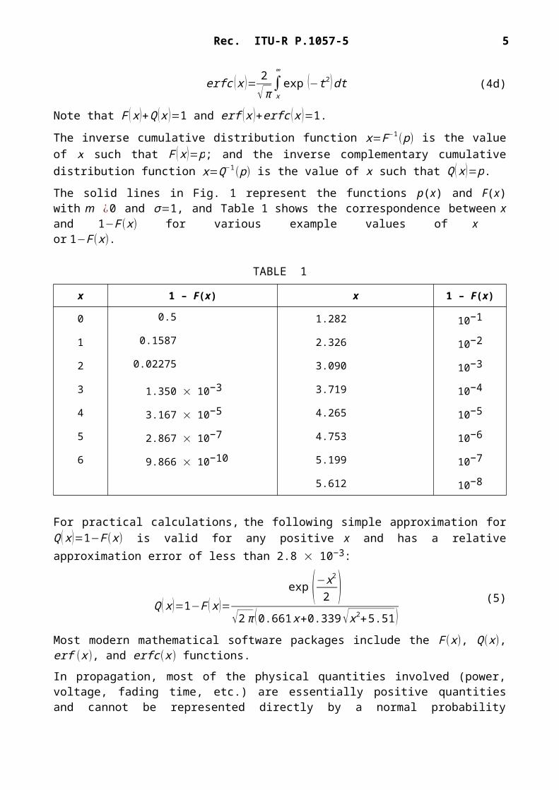
The solid lines in Fig. 1 represent the functions p(x) and F(x) with m ¿0 and σ=1, and Table 1 shows the correspondence between x and 1−F (x) for various example values of x or 1−F (x).

TABLE 1

x 1 – F(x) x 1 – F(x)

0 0.5 1.282 10−1

1 0.1587 2.326 10−2

2 0.02275 3.090 10−3

3 1.350 10−3 3.719 10−4

4 3.167 10−5 4.265 10−5

5 2.867 10−7 4.753 10−6

6 9.866 10−10 5.199 10−7

5.612 10−8

For practical calculations, the following simple approximation for Q ( x )=1−F (x) is valid for any positive x and has a relative approximation error of less than 2.8 10−3:

Q ( x )=1−F ( x )=exp (−x2

2 )√2π (0.661 x+0.339√x2+5.51 )

(5)

Most modern mathematical software packages include the F (x), Q(x ), erf (x), and erfc (x) functions.

In propagation, most of the physical quantities involved (power, voltage, fading time, etc.) are essentially positive quantities and cannot be represented directly by a normal probability distribution. The normal probability distribution is used in two important cases:– to represent the fluctuations of a random variable around its mean value

(e.g. scintillation fades and enhancements);– to represent the fluctuations of the logarithm of a random variable, in which case the

variable has a log-normal probability distribution (see § 4).

Diagrams in which one of the coordinates is a so-called normal coordinate, where a normal cumulative probability distribution is represented by a straight line, are available commercially. These diagrams are frequently used even for the representation of non-normal probability distributions.

Rec. ITU-R P.1057-5 5

4 Log-normal probability distribution

The log-normal probability distribution is the probability distribution of a positive random variable X whose natural logarithm has a normal probability distribution. The probability density function, p ( x ) , and the cumulative distribution function, F (x), are:

p( x )= 1σ √2 π

1x

exp [−12 (ln x−m

σ )2]

(6)

F (x )= 1σ √2 π ∫0

x1t

exp [−12 ( ln t−m

σ )2 ] dt =1

2 [1 + erf ( ln x−mσ √2 )]

(7)

where m and are the mean and the standard deviation of the logarithm of X (i.e. not the mean and the standard deviation of X).

The log-normal probability distribution is very often found in propagation probability distributions associated with power and field-strength. Since power and field-strength are generally expressed in decibels, their probability distributions are sometimes incorrectly referred to as normal rather than log-normal. In the case of probability distributions vs. time (e.g. fade duration in seconds), the log-normal terminology is always used explicitly because the natural dependent variable is time rather than the logarithm of time.

Since the reciprocal of a variable with a log-normal probability distribution also has a log-normal probability distribution, this probability distribution is sometimes found in the case of the probability distribution of the rate of change (e.g. fading rate in dB/s or rainfall rate in mm/hr).

In comparison with a normal probability distribution, a log-normal probability distribution is usually encountered when values of the random variable of interest results from the product of other approximately equally weighted random variables.

Unlike a normal probability distribution, a log-normal probability distribution is extremely asymmetrical. In particular, the mean value, the median value, and the most probable value (often called the mode) are not identical (see the dashed lines in Fig. 1).

The characteristic values of the random variable X are: – most probable value: exp (m – 2);– median value: exp (m);

– mean value:exp (m+ σ2

2 );

– root mean square value: exp (m + 2);

– standard deviation:exp (m+ σ2

2 ) √exp (σ2 )−1.

6 Rec. ITU-R P.1057-5

FIGURE 1Normal and log-normal probability distributions

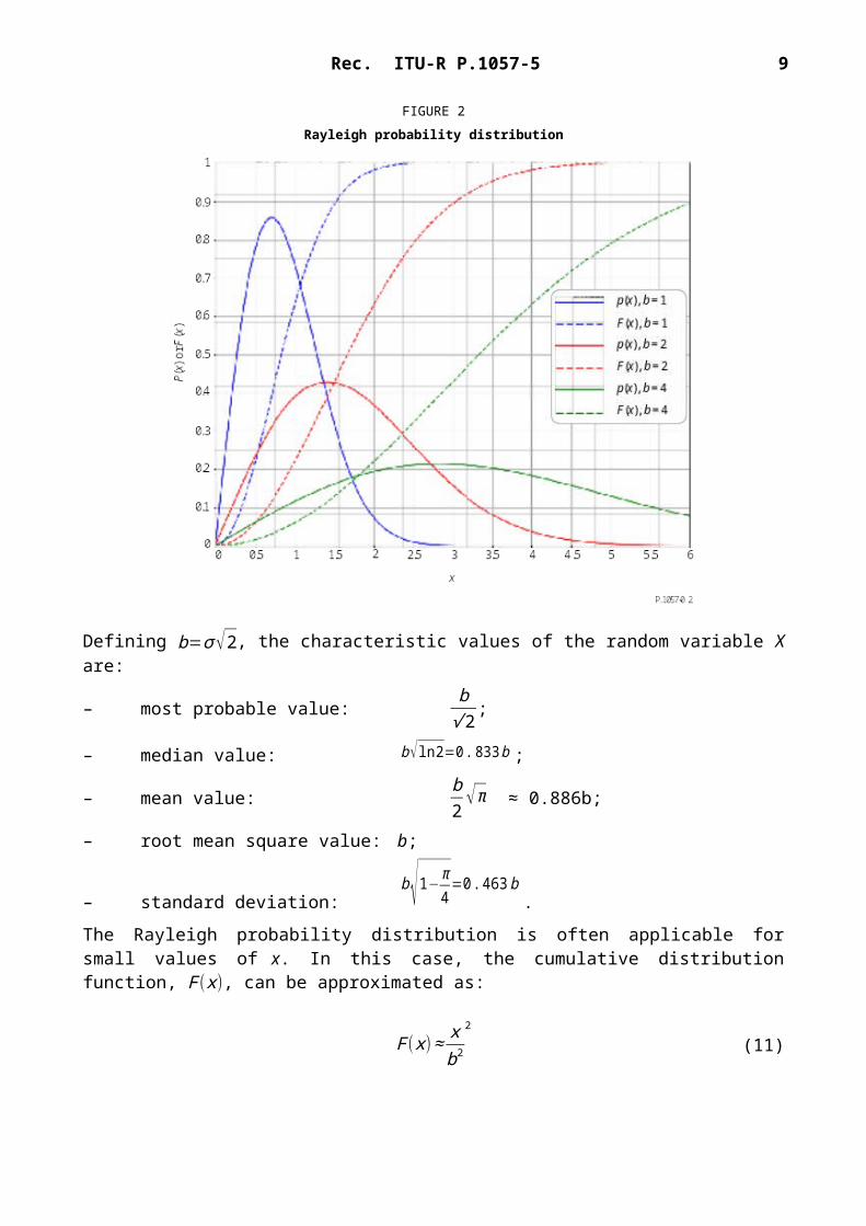
5 Rayleigh probability distribution

The Rayleigh probability distribution is a continuous probability distribution of a positive-valued random variable. For example, given a two-dimensional normal probability distribution with two independent random variables y and z of mean zero and the same standard deviation , the random variable

x=√ y2+z2(8)

has a Rayleigh probability distribution. The Rayleigh probability distribution also represents the probability distribution of the length of a vector that is the vector sum of a large number of constituent vectors of similar amplitudes where the phase of each constituent vector has a uniform probability distribution.

The probability density function and the cumulative distribution function of a Rayleigh probability distribution are given by:

p( x ) = xσ2 exp (− x2

2 σ 2 )(9)

F (x )= 1−exp (− x2

2 σ 2)(10)

Figure 2 provides examples of p(x) and F(x) for three different values of b.

Rec. ITU-R P.1057-5 7

FIGURE 2Rayleigh probability distribution

Defining b=σ √2, the characteristic values of the random variable X are:

– most probable value:b

√ 2 ;

– median value: b√ ln 2=0. 833 b ;

– mean value:b2 √π ≈ 0.886b;

– root mean square value: b;

– standard deviation:b√1− π

4=0 . 463b

.

The Rayleigh probability distribution is often applicable for small values of x. In this case, the cumulative distribution function, F (x), can be approximated as:

F (x)≈ xb2

2

(11)

This approximate expression can be interpreted as follows: the probability that the random variable X will have a value less than x is proportional to the square of x. If the variable of interest is a voltage, its square represents the power of the signal. In other words, on a decibel scale the power decreases by 10 dB for each decade of probability. This property is often used to determine whether a received level has an asymptotic Rayleigh probability distribution. Note, however, that other probability distributions can have the same behaviour.

8 Rec. ITU-R P.1057-5

In radiowave propagation, a Rayleigh probability distribution occurs in the analysis of scattering from multiple, independent, randomly-located scatterers for which no single scattering component dominates.

6 Combined log-normal and Rayleigh probability distribution

In some cases, the probability distribution of a random variable can be regarded as the combination of two probability distributions; i.e. a log-normal probability distribution for long-term (i.e. slow) variations and a Rayleigh probability distribution for short-term (i.e. fast) variations. This probability distribution occurs in radiowave propagation analyses when the inhomogeneities of the propagation medium have non-negligible long-term variations; e.g. in the analysis of tropospheric scatter.

The instantaneous probability distribution of the random variable is obtained by considering a Rayleigh probability distribution whose mean (or mean square) value is itself a random variable having a log-normal probability distribution.

The probability density function of the combined log-normal and Rayleigh probability distribution is:

p ( x )=√ 2π

kx∫−∞

∞

exp(−k x2 exp (−2 (σ u+m ) )−2 (σ u+m)−u2

2 )d u (12a)

and the complementary cumulative distribution function of the combined log-normal and Rayleigh probability distribution is:

1−F (x )= 1√2π ∫−∞

∞

exp(−k x2 exp (−2 (σ u+m ) )−u2

2 )du (12b)

where m and , expressed in nepers, are the mean and the standard deviation of the normal probability distribution associated with the log-normal distribution.

The value of k depends on the interpretation of σ and m:1) If σ and m are the standard deviation and mean of the natural logarithm of the most

probable value of the Rayleigh probability distribution, then k=1/2;2) if σ and m are the standard deviation and mean of the natural logarithm of the median value

of the Rayleigh probability distribution, then k=ln 2;3) if σ and m are the standard deviation and mean of the natural logarithm of the mean value

of the Rayleigh probability distribution, then k=π /4; and4) if σ and m are the standard deviation and mean of the natural logarithm of the root mean

square value of the Rayleigh probability distribution, then k=1.

The mean (E), root mean square (RMS), standard deviation (SD), median, and most probable value of the combined Rayleigh log-normal probability distribution are:

Mean value, E

E=∫0

∞

x√ 2π

kx [∫−∞

∞

exp (−k x2 [−2 (σ u+m ) ]−2 (σ u+m )−u2

2 )du]dx (13a)

¿ √π2√k

exp(m+ σ2

2 ) (13b)

Rec. ITU-R P.1057-5 9

Root mean square value, RMS

RMS=√∫0∞ x2√ 2π kx [∫

−∞

∞

exp(−k x2 exp [−2 (σ u+m ) ]−2 (σ u+m )−u2

2 )du]dx (13c)

¿ 1√k

exp (m+σ2) (13d)

Standard deviation, SD

SD=√ 1k

exp (2 (m+σ 2 ))− π4 k

exp (2(m+ σ2

2 )) (13e)

¿ 1√k

exp(m+ σ 2

2 )√exp (σ2 )− π4

(13f)

Median value

The median value is the value of x that is the solution of:

12=1− 1

√2 π ∫−∞

∞

exp(−k x2 exp (−2 (σ u+m ) )− u2

2 )du (13g)

i.e.

√ π2=∫

−∞

∞

exp(−k x2exp (−2 (σ u+m ) )−u2

2 )du (13h)

Most probable value

The most probable value (i.e. the mode) is the value of x that is the solution of:

∫−∞

∞ {1−2 kx 2 exp [−2 (σu+m ) ] }exp {−kx 2exp [−2 (σu+m ) ]−2 (σu+m )−u2

2 }du=0(13i)

Figure 3 shows a graph of this probability distribution for several values of the standard deviation, where m=0, and k=1 .

10 Rec. ITU-R P.1057-5

FIGURE 3Combined log-normal and Rayleigh probability distributions (with standard deviation of the

log-normal probability distribution as a parameter)

7 Nakagami-Rice (Nakagami n) probability distribution

The Nakagami-Rice (Nakagami n) probability distribution, which is different than the Nakagami m probability distribution, is a generalization of the Rayleigh probability distribution. It may be considered as the probability distribution of the length of a vector that is the sum of a fixed vector and a vector whose length has a Rayleigh probability distribution.

Alternatively, given a two-dimensional normal probability distribution with two independent variables x and y with the same standard deviation , the length of a vector joining a point in the probability distribution to a fixed point different from the centre of the probability distribution has a Nakagami-Rice probability distribution.

If a designates the length of the fixed vector and the most probable length of the Rayleigh vector, the probability density function is:

Rec. ITU-R P.1057-5 11

p( x )= xσ 2 exp (− x2+ a2

2 σ2 ) I 0 ( a xσ2 )

(14)

where I0 is the modified Bessel function of the first kind and of zero order.

This probability distribution depends on the ratio between the amplitude of the fixed vector a, and the root mean square amplitude of the random vector, σ √2 . There are two main radiowave propagation applications as follows:a) The power in the fixed vector is constant, but the total power in the fixed and random

components is a random probability distribution.

For studies of the influence of a ray reflected by a rough surface, or for consideration of multipath

components in addition to a fixed component, the mean power is given by (a2+2 σ2 ) . The probability distribution is often defined in terms of a parameter K:

K = 10 log ( a2

2 σ 2 )            dB (15)

which is the ratio of the powers in the fixed vector and the random component.b) The total power in the fixed and random components is constant, but both components

vary.

For the purpose of studying multipath propagation through the atmosphere, it can be considered that the sum of the power carried by the fixed vector and the mean power carried by the random vector is constant since the power carried by the random vector originates from the fixed vector. If the total power is taken to be unity, then:

a2+2 σ2=1 (16)

and the fraction of the total power carried by the random vector is then equal to 2 σ2 . If X is the resultant vector random variable, the probability that the random variable X is greater than x is:

Prob (X > x) = 1 – F(x) = 2 exp (− a2

2 σ 2) ∫x /σ√2

∞

νexp (−ν2) I 0( 2νaσ √2 ) dν

(17)

Figure 4 shows this probability distribution for different values of the fraction of power carried by the random vector.

12 Rec. ITU-R P.1057-5

FIGURE 4Nakagami-Rice probability distribution for a constant total power (with the fraction of power

carriedby the random vector as parameter)

For practical applications amplitudes are displayed using a decibel scale, and probabilities are displayed using a scale where a Rayleigh cumulative probability distribution is a straight line. For values of the fraction of the total power in the random vector above approximately 0.5, the curves asymptotically approach a Rayleigh probability distribution because the fixed vector has an amplitude of the same order of magnitude as that of the random vector, and the fixed vector is practically indistinguishable from the random vector. In comparison, for small values of this fraction of the total power in the random vector, the amplitude probability distribution tends towards a normal probability distribution.

While the amplitude has a Nakagami-Rice probability distribution, the probability density function of the phase is:

Rec. ITU-R P.1057-5 13

p(θ )= 12 π {1+√ π

2a cosθ

σe

a2cos2θ2 σ2 [1+erf( a cosθ

√2 σ )]}⋅e− a2

2σ 2

(18)

8 Gamma probability distribution and exponential probability distribution

Unlike the previous probability distributions that are derived from a normal probability distribution, the gamma probability distribution is a generalization of the exponential probability distribution. It is the probability distribution of a positive and non-limited variable. The probability density function is:

p( x )= α ν

Γ ( ν )xν−1 e−α x

(19)

where Γ is the Euler function of second order.

This cumulative distribution function depends on two parameters and . However, is only a scale parameter of variable x. The characteristic values of the random variable X are:

– mean value: να

– root mean square value:√ν (1+ν )

α

– standard deviation:√να

The integral expressing the cumulative distribution function cannot be evaluated in closed form except for integer values of . The following are series expansions for two special cases:

A series approximation for x << 1:

F (x )= 1Γ ( ν+1)

e−α x (α x )ν [1+ α xν+1

+(α x )2

(ν+1 ) (ν+2 )+. .. .]

(20)

An asymptotic approximation for x 1 is:

1−F ( x )= 1Γ (ν )

e−α x ( α x )ν−1[1+ ν−1α x

+(ν−1 ) (ν−2)

(α x )2+ .. ..]

(21)

For equal to unity, F (x) becomes an exponential probability distribution. For integer , the asymptotic expansion has a finite number of terms and gives the gamma probability distribution in an explicit form.

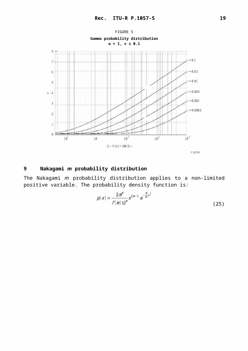
In radiowave propagation, the useful values of are very low values of the order of 1 × 10−2 to 1 × 10−4. For  near zero:

14 Rec. ITU-R P.1057-5

1Γ (ν )

~ νΓ ( ν + 1)

~ ν(22)

in which case, for x > 0.03:

1−F ( x ) ~ ν ∫α x

∞ e−t

td t

(23)

For practical calculations, it is possible to approximate the above integral as:

1−F ( x ) ~ ν e−α x

0 .68+α x+0 .28 log α x (24)

which is valid for < 0.1 and x 0.03.

The cumulative distribution function of the complementary gamma function for small values of is shown in Fig. 5. The probability of the variable X being significantly greater than zero is always small. In particular, this explains the use of the gamma probability distribution to represent rainfall rates since the total percentage of rainfall time is generally of the order of 2 to 10%.

FIGURE 5Gamma probability distribution

α = 1, ν ≤ 0.1

9 Nakagami m probability distribution

The Nakagami m probability distribution applies to a non-limited positive variable. The probability density function is:

Rec. ITU-R P.1057-5 15

p( x ) = 2 mm

Γ (m) Ωm x2m−1 e−mΩ x2

(25)

16 Rec. ITU-R P.1057-5

Ω is a scale parameter equal to the mean value of x2; i.e.

x2=Ω (26)

where m is a parameter of the Nakagami m probability distribution and not a mean value as in previous sections of this Annex.

This probability distribution is related to other probability distributions as follows:– if a random variable has a Nakagami m probability distribution, the square of the random

variable has a gamma probability distribution;– for m = 1 the Nakagami m probability distribution becomes a Rayleigh probability

distribution;– for m = 1/2 the Nakagami m probability distribution becomes a one-sided normal

probability distribution.

The Nakagami m probability distribution and the Nakagami-Rice probability distribution are two different generalizations of the Rayleigh probability distribution. For very low signal levels, the slope of the Nakagami m probability distribution tends towards a value which depends on the parameter m, unlike the Nakagami-Rice probability distribution where the limit slope is always the same (10 dB per decade of probability). The cumulative Nakagami m probability distribution for various values of the parameter m is shown in Fig. 6.

Rec. ITU-R P.1057-5 17

FIGURE 6

Nakagami-m probability distribution (x2=1)

18 Rec. ITU-R P.1057-5

10 Pearson 2 probability distribution

The Pearson χ2 probability density function is:

p( χ2 )= 1

2ν2 Γ ( ν

2 )e− χ2

2 ( χ2)ν2

– 1

(27)

where 2 is a non-limited positive variable, and the parameter , a positive integer, is the number of degrees of freedom of the probability distribution. Γ represents the Euler function of second order. Depending on the parity of , one has

even:Γ ( ν

2 )=( ν2−1) !

(28)

odd:Γ ( ν

2 )=( ν2−1) ( ν

2−2) .. . 1

2 √π(29)

The cumulative distribution function is:

F ( χ2 )= 1

2ν2 Γ ( ν

2 )∫0

χ2

e− t

2 tν2− 1

dt

(30)

The mean and standard deviation are:

m=ν (31)

σ=√2 ν (32)

An essential property of the 2 probability distribution is that, if n variables xi {i=1, 2, … , n} have Gaussian probability distributions with mean mi and standard deviation i, the variable:

∑i=l

n ( xi−mi

σ i)2

(33)

has a 2 probability distribution of n degrees of freedom. In particular, the square of a small Gaussian variable has a 2 probability distribution of one degree of freedom.

If several independent variables have 2 probability distributions, their sum also has a 2 probability distribution with the number of degrees of freedom equal to the sum of the degrees of freedom of each variable.

The 2 probability distribution is not fundamentally different from the gamma probability distribution. The two probability distributions are related by:

χ2

2=α x

(34)ν2=n

(35)

Rec. ITU-R P.1057-5 19

Similarly, the 2 probability distribution is related to the Nakagami-m probability distribution by:χ2

2=mΩ x2

(36)

ν2=m

(37)

The 2 probability distribution is used in statistical tests to determine whether a set of experimental values of a quantity (e.g. rainfall rate, attenuation, etc.) can be modelled by a given statistical probability distribution.

Figure 7 gives a graphic representation of the χ2 probability distribution for several values of .

20 Rec. ITU-R P.1057-5

FIGURE 72 probability distribution

Rec. ITU-R P.1057-5 21

Annex 2

Step-by-step procedure to approximate a complementary cumulative distribution by a log-normal complementary cumulative distribution

1 Background

The log-normal cumulative distribution is defined as:

F (x )= 1σ √2 π ∫0

x 1t

exp [−12 ( ln t−m

σ )2] dt

¿12 [1 + erf ( ln x−m

σ √2 )] (38)

or equivalently:

F (x )= 1√2π ∫

−∞

ln x−mσ

exp [− t2

2 ] dt(39)

Similarly, the log-normal complementary cumulative distribution is defined as:

G( x ) = 1σ √2π ∫

x

∞ 1t

exp [−12 ( ln t−m

σ )2 ] dt

¿12

erfc ( ln x−mσ √2 )=1

2 [1−erf ( ln x−mσ √2 )]

(40)

or equivalently:

G( x ) = 1√2 π ∫

ln x−mσ

∞

exp [−t2

2 ] dt

¿Q( ln x−mσ ) (41)

where Q ( . ) is the normal complementary cumulative probability integral. The parameters m and can be estimated from the set of n pairs (Gi, xi) as described in the following paragraph.

22 Rec. ITU-R P.1057-5

2 Procedure

Estimate the two log-normal parameters m and as follows:

Step 1: Construct the set of n pairs (Gi, xi), where Gi is the probability that xi is exceeded.

Step 2: Transform the set of n pairs from (Gi, xi) to (Zi, ln xi) where:

Zi=√2erf c−1 (2 Gi )=√2 erf −1(1−2 Gi) or equivalently, Zi=Q−1(Gi)

Step 3: Determine the variables m and σ by performing a least squares fit to the linear function:

ln xi=σ Z i+m

as follows:

σ=n ∑

i=1

n

Z i ln xi −∑i=1

n

Z i ∑i=1

n

ln x i

n ∑i=1

n

Zi2−[∑i=1

n

Z i ]2

m=∑i=1

n

ln x i−σ ∑i=1

n

Z i

n