Temperature Sensors & Measurement

E80 Spring 2014

Contents

Why measure temperature?

Characteristics of interest

Types of temperature sensors– 1. Thermistor– 2. RTD Sensor– 3. Thermocouple– 4. Integrated Silicon Linear Sensor

Sensor Calibration

Signal Conditioning Circuits (throughout)

Why Measure Temperature?

Temperature measurements are one of the most common measurements...

Temperature corrections for other sensors – e.g., strain, pressure, force, flow, level, and position many

times require temperature monitoring in order to insure accuracy.

Important Properties?

Sensitivity

Temperature range

Accuracy

Repeatability

Relationship between measured quantity and temperature

Linearity

Calibration

Response time

Types of Temperature Sensors?

Covered1. Thermistor

Ceramic-based: oxides of manganese, cobalt , nickel and copper

2. Resistive Temperature Device -RTDMetal-based : platinum, nickel or

copper

3. Thermocouplejunction of two different metals

4. Integrated Silicon Linear SensorSi PN junction of a diode or

bipolar transistor

5

Not Covered5. Hot Wire Anemometer

6. Non-Contact IR Single Sensor

7. IR Camera

>$10

Part I Thermistor

High sensitivity

Inexpensive

Reasonably accurate

Lead resistance ignored

Glass bead, disk or chip thermistor

Typically Negative Temperature Coefficient (NTC),– PTC also possible

nonlinear relationship between R and T

Thermistor resistance vs temperature

Simple Exponential Thermistor Model 

RT = R0 x exp[ β(1/T -1/T0)]

– RT is the thermistor resistance (Ω).

– T is the thermistor temperature (K)

– Manufacturers will often give you R0, T0 and an average value for β

• β  is a curve fitting parameter and itself is temperature dependent.

Simple Exponential Thermistor Model

Usually T0 is room temp 25oC = 298oK– So R0 = R25

RT = R25 x exp[β(1/T – 1/298)]

– where β ≈ ln (R85/R25) /(1/358-1/298)

Not very accurate but easy to use

Better Thermistor model

Resistance vs temperature is non-linear but can be well characterised by a 3rd order polynomial

ln RT = A + B / T +C / T2 + D / T3

where A,B,C,D are the characteristics of the material used.

Inverting the equation

The four term Steinhart-Hart equation

T = [A1 +B1 ln(RT/R0)+C1 ln2(RT/R0)+D1ln3(RT/R0)]-1

Also note: • Empirically derived polynomial fit• A, B, C & D are not the same as A1, B1 , C1 & D1

• Manufacturers should give you both for when R0 = R25

• C1 is very small and sometime ignored (the three term SH eqn)

http://www.eng.hmc.edu/NewE80/PDFs/VIshayThermDataSheet.pdf

Thermistor Calibration

3-term Steinhart-Hart equation

T = [A1 +B1 ln(RT/R0)+D1ln3(RT/R0)]-1

How do we find A1, B1 and D1?

Minimum number of data points?

Linear regression/Least Squares Fit (Lecture 2)

Thermistor Problems: Self-heating

You need to pass a current through to measure the voltage and calculate resistance.

Power is consumed by the thermistor and manifests itself as heat inside the device– P = I2 RT

– You need to know how much the temp increases due to self heating by P so you need to be given θ = the temperature rise for every watt of heat generated.

Heat flow

Very similar to Ohms law. The temperature difference (increase or decrease) is related to the power dissipated as heat and the thermal resistance.

Δ C = P x θ

– P in Watts– θ in oC /W

Self Heating Calculation

ΔoC = P x θ = (I2 RT) θ Device to ambient

Example. – I = 5mA – RT = 4kΩ

– θDevice to ambient = 15 oC /W

ΔoC =

Self Heating Calculation

ΔoC = P x θ = (I2 RT) θ Device to ambient

Example. – I = 5mA – RT = 4kΩ

– θDevice to ambient = 15 oC /W

ΔoC = (0.005)2 X 4000 X 15 = 1.5 C

Linearization Techniques

Current through Thermistor is dominated by 10k Ω resistor.

Linearization of a 1O k-Ohm Thermistor

This plot Ti = 50 0C, Ri = 275 Ω

Linearization techniques

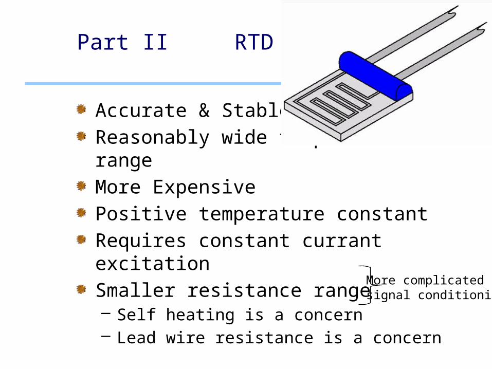
Part II RTD

Accurate & Stable

Reasonably wide temperature range

More Expensive

Positive temperature constant

Requires constant currant excitation

Smaller resistance range– Self heating is a concern– Lead wire resistance is a concern

More complicatedsignal conditioning

pRTD, cRTD and nRTD

The most common is one made using platinum so we use the acronym pRTD

Copper and nickel as also used but not as stable

Linearity: The reason RTDs are so popular

RTD are almost linear

Resistance increases with temperature (+ slope)

RT = R0(1+ α)(T –T0)

Recognized standards for industrial platinum RTDs are– IEC 6075 and ASTM E-1137 α = 0.00385 Ω/Ω/°C

Measuring the resistanceneeds a constant current source

Read AN 687 for more details (e.g. current excitation circuit): http://ww1.microchip.com/downloads/en/AppNotes/00687c.pdfhttp://www.control.com/thread/1236021381on 3-wire RTD

With long wires precision is a problem

Two wire circuits,

Three wire circuits and

Four wire circuits.

Two wire: lead resistances are a problem

The IDAC block is a constant current sink

Power supply connected here

No current flows in here

Three wire with two current sinks

Four wire with one current sink.

4 wire with precision current source

Mathematical Modelling the RTD

The Callendar-Van Dusen equation

RT = R0 (1 + A T + B T2 + C T3(T-100) for T < 0 oC

= R0 (1+ A T + B T2) for T > 0 oC– where R0 is the resistance at T0 = 0 oC and

For platinum

A = 3.9083 x e-3 oC-1

B = -5.775 x e-7 oC-2

C = -4.183 x e-12 oC-4

Experimentally

Derive temperature (+/-) from the measured resistance.

Easiest way is to construct a Look-Up table inside LabView or your uP

Precision, accuracy, errors and uncertainties need to be considered.

Experimental uncertainties

For real precision, each sensor needs to be calibrated at more than one temperature and any modelling parameters refined by regression using a least mean squares algorithm. – LabView, MATLAB and Excel have these functions

The 0oC ice bath and the ~100 oC boiling de-ionised water (at sea level) are the two most convenient standard temperatures.

Part III Thermocouples

High temperature range

Inexpensive

Withstand tough environments

Multiple types with different temperature ranges

Requires a reference temperature junction

Fast response

Output signal is usually small

Amplification, noise filtration and signal processing required

Seebeck Effect

Type K thermocouple

Thermocouples are very non-linear

Mathematical Model

To cover all types of thermocouples, we need a 6 - 10th order polynomial to describe the relationship between the voltage and the temperature difference between the two junctions

Either

T = a0 +a1 x V + a2 x V2 +++++ a10 V10

Or

V = b0 +b1 x T + b2 x T2 +++++ b10 T10

+ αo exp(α1(T-126.9686)2) for T >0oC

10th order polynomial fit:Find T from measured Voltage

What happens when we connect a meter?

What happens when we connect a meter?

Cu

Cu

Cold Junction Compensation

Can we read the voltage directly from our DAQ or meter?

Instrumentation Amplifier

One more thing…

Low voltage signal…

Long leads…

What problems could arise?

Thermocouple with compensation and filtering

Look-up table is easier than using a polynomial

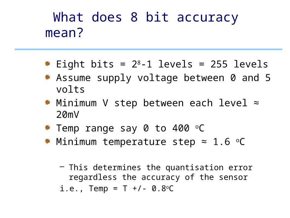
What does 8 bit accuracy mean?

Eight bits = 28-1 levels = 255 levels

Assume supply voltage between 0 and 5 volts

Minimum V step between each level ≈ 20mV

Temp range say 0 to 400 oC

Minimum temperature step ≈ 1.6 oC

– This determines the quantisation error regardless the accuracy of the sensor

i.e., Temp = T +/- 0.8oC

Part IV Silicon Detectors

Integrated form

-40°C to +150°C

Limited accuracy +/- 2 degree

Linear response ( no calibration is required)

Direct interface with ADC

References

Previous years’ E80

Wikipedia

Microchip Application Notes AN679, AN684, AN685, AN687

Texas Instruments SBAA180

Omega Engineering www.omega.com (sensor specs, application guides, selection guides, costs)

Baker, Bonnie, “Designing with temperature sensors, part one: sensor types,” EDN, Sept 22, 2011, pg 22.

Baker, Bonnie, “Designing with temperature sensors, part two: thermistors,” EDN, Oct 20, 2011, pg 24.

Baker, Bonnie, “Designing with temperature sensors, part three: RTDs,” EDN, Nov 17, 2011, pg 24.

Baker, Bonnie, “Designing with temperature sensors, part four: thermocouples,” EDN, Dec 15, 2011, pg 24.

Baker, Bonnie, “Designing with temperature sensors, part one: sensor types,” EDN, Sept 22, 2011, pg 22.

Baker, Bonnie, “Designing with temperature sensors, part two: thermistors,” EDN, Oct 20, 2011, pg 24.

Baker, Bonnie, “Designing with temperature sensors, part three: RTDs,” EDN, Nov 17, 2011, pg 24.

Baker, Bonnie, “Designing with temperature sensors, part four: thermocouples,” EDN, Dec 15, 2011, pg 24.