Tehcnical Paper: Calculating Freezing Times in Blast and Plate Freezers by Dr. Andy Pearson

Technical Papers31st Annual Meeting

International Institute of Ammonia Refrigeration

March 22–25, 2009

2009 Industrial Refrigeration Conference & ExhibitionThe Hyatt Regency

Dallas, Texas

ACKNOWLEDGEMENT

The success of the 31st Annual Meeting of the International Institute of Ammonia

Refrigeration is due to the quality of the technical papers in this volume and the labor of its

authors. IIAR expresses its deep appreciation to the authors, reviewers and editors for their

contributions to the ammonia refrigeration industry.

Board of Directors, International Institute of Ammonia Refrigeration

ABOUT THIS VOLUME

IIAR Technical Papers are subjected to rigorous technical peer review.

The views expressed in the papers in this volume are those of the authors, not the

International Institute of Ammonia Refrigeration. They are not official positions of the

Institute and are not officially endorsed

International Institute of Ammonia Refrigeration

1110 North Glebe Road

Suite 250

Arlington, VA 22201

+ 1-703-312-4200 (voice)

+ 1-703-312-0065 (fax)

www.iiar.org

2009 Industrial Refrigeration Conference & Exhibition

The Hyatt Regency

Dallas, Texas

© IIAR 2009 1

Technical Paper #5

Calculating Freezing Times in Blast and Plate Freezers

Dr. Andy PearsonStar Refrigeration Ltd

Glasgow, UK

Abstract

Recent experiences using carbon dioxide have shown remarkable improvements in freezing times. Close analysis of the freezing process has shown that this improvement is a result of the elimination of hindrances which handicap traditional freezer designs such as high suction line pressure drops, intolerance of off-design operation and internal fouling. The paper presents several methods of modeling the freezing process which can be used in a simple spreadsheet, and which help to explain the benefits which can be gained by using a correctly designed system with carbon dioxide as the refrigerant.

The paper will provide an explanation of the theory behind the freezing process and will convert this into a methodology which can be implemented in a standard spreadsheet. For more advanced users the option of automating the spreadsheet by using macro programs will be explained.

2009 IIAR Industrial Refrigeration Conference & Exhibition, Dallas, Texas

Technical Paper #5 © IIAR 2009 3


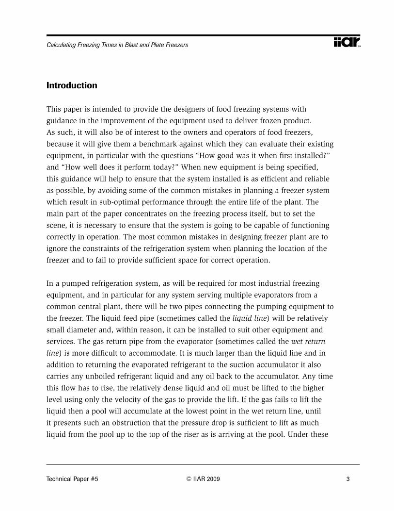
Introduction

This paper is intended to provide the designers of food freezing systems with

guidance in the improvement of the equipment used to deliver frozen product.

As such, it will also be of interest to the owners and operators of food freezers,

because it will give them a benchmark against which they can evaluate their existing

equipment, in particular with the questions “How good was it when first installed?”

and “How well does it perform today?” When new equipment is being specified,

this guidance will help to ensure that the system installed is as efficient and reliable

as possible, by avoiding some of the common mistakes in planning a freezer system

which result in sub-optimal performance through the entire life of the plant. The

main part of the paper concentrates on the freezing process itself, but to set the

scene, it is necessary to ensure that the system is going to be capable of functioning

correctly in operation. The most common mistakes in designing freezer plant are to

ignore the constraints of the refrigeration system when planning the location of the

freezer and to fail to provide sufficient space for correct operation.

In a pumped refrigeration system, as will be required for most industrial freezing

equipment, and in particular for any system serving multiple evaporators from a

common central plant, there will be two pipes connecting the pumping equipment to

the freezer. The liquid feed pipe (sometimes called the liquid line) will be relatively

small diameter and, within reason, it can be installed to suit other equipment and

services. The gas return pipe from the evaporator (sometimes called the wet return

line) is more difficult to accommodate. It is much larger than the liquid line and in

addition to returning the evaporated refrigerant to the suction accumulator it also

carries any unboiled refrigerant liquid and any oil back to the accumulator. Any time

this flow has to rise, the relatively dense liquid and oil must be lifted to the higher

level using only the velocity of the gas to provide the lift. If the gas fails to lift the

liquid then a pool will accumulate at the lowest point in the wet return line, until

it presents such an obstruction that the pressure drop is sufficient to lift as much

liquid from the pool up to the top of the riser as is arriving at the pool. Under these

4 © IIAR 2009 Technical Paper #5


conditions the pool will be stable, but if the load changes, as happens frequently

in freezer plants, or if the operating conditions shift to higher or lower temperature

then the stable operation will be disrupted and the system will have to find a new

balance point. This shift in operating point can introduce numerous difficulties to

the operation. There may be a tidal wave of liquid returning occasionally to the

accumulator at high velocity and possibly causing damage to valves, fittings or

pipework. Defrost might be more difficult to achieve because of the volume of liquid

held in the suction line. The amount of oil held in the wet return line might also

compromise plant efficiency and reliability, as well as requiring skilled maintenance

to keep the plant operating. Most significantly, the amount of pressure drop needed

to lift the liquid could, in extreme cases, be as much as a 10K (18°F) drop in the

saturated suction temperature, making the plant inefficient and possibly under

capacity.

Location of the freezer and associated equipment plays a large part in enabling the

refrigeration system to work well. Often the freezer location is decided very early

in the project, when the factory layout is being established, but the position of the

refrigeration machinery room is not finalised until the last minute, and it is often put

in the only space left; far away from the production area. This is not necessarily a

problem provided the wet return pipe can be installed to drain all the way from the

freezer to the accumulator, but often the distance is too great, the height difference

is too small or other services and equipment have already been installed in the way.

Any interruption of the drain path with a rise in the pipe will require additional

pressure loss to lift the liquid, and will reduce the plant efficiency. In extreme cases,

where the wet suction line pressure loss is too large, it may be possible to install the

accumulator and pumps close to the freezer, either in the production area or else in

a nearby yard or light well, so that the liquid overfeed can drain back to the pumps.

The pipe from the accumulator back to the compressors then becomes a dry return,

so can rise and fall as required by the constraints of the building. It may still be

necessary to consider oil return in the dry suction, unless oil is recovered from the

local accumulator. It may also be necessary to install additional safety precautions



such as ventilation, gas sensors and alarms to ensure production staff safety and to

meet code requirements.

The relatively high pressure and high gas density of carbon dioxide at the freezer’s

operating temperature offer the possibility of improved freezer performance by

reducing the drop in saturation temperature between the evaporator and the

compressor. Thus for a given suction gas condition at the compressor the evaporation

in the freezer will be at a lower temperature with carbon dioxide as the refrigerant

than it would be with ammonia. This is particularly important in plate freezer

systems with high pumped overfeed rates, where the drop in saturation temperature

between the plate outlet and the suction header can be as high as 10K (18°F). On the

other hand ammonia provides better coefficients of heat transfer than carbon dioxide,

by a factor of between 2 and 4, according to Stoecker (2000) and Hrnjak and Park

(2007).

The performance of plate and blast freezers has been explored in two previous

papers by the author. In the first, presented to the International Institute of Ammonia

Refrigeration’s annual meeting in Acapulco, in 2005, the beneficial effect of using

carbon dioxide in vertical plate freezers was described. In the plant in question

75mm slabs of wet meat products were frozen in an automated system which had

originally been designed with a two-hour cycle time, including five minutes for

defrosting, five minutes for unloading and ten minutes for loading the next batch.

The design was based on a calculated freezing time of ninety-five minutes, allowing

a further five minutes leeway in the two-hour cycle. However, on-site measurements

showed that the core of the slab was achieving the required temperature in fifty-

eight minutes. The plant operator was able to raise the compressor suction pressure

setpoint of the plant from –50°C (–58°F) to –43°C (–45°F), thereby improving the

plant efficiency by about 20%. In the second paper, presented to the International

Institute of Refrigeration’s Gustav Lorentzen Conference in Copenhagen in 2008, an

analysis of a multi-chamber blast freezer was presented. This showed that a similar

benefit had been achieved in a multi-chamber blast freezer where the product, boxed



beef, was frozen to a core temperature of –18°C (0°F) in an airstream nominally

at –38°C (–36°F). Compared with a calculated freezing time of 22 hours for the

blast freezer, product was frozen to a core temperature of –18°C within 18 hours, a

reduction of 18%. The boxes in this study were 600mm (23.5") by 390mm (15.5") by

150mm (6").

The question suggested by these field experiences is whether the improved

performance is a direct consequence of the use of carbon dioxide as the refrigerant,

or just the result of good practice in the management of the freezing process on the

sites in question.

To provide a better understanding of these benefits, a more detailed model of

the freezing process was developed. This was designed to be simple enough to

implement in a spreadsheet, yet containing sufficient accuracy in food properties to

provide an insight into the freezing process that would explain the unexpectedly good

results. This model of freezing could then be combined with a model of evaporator

performance in order to investigate, for example, the differences between ammonia

systems and carbon dioxide systems.

The Freezing Process

According to the United Nations Environment Program (UNEP, 2006), the global

market for frozen food is about 40 million tonnes (44 million tons) per year,

compared to a chilled food market of about 350 million tonnes (385 million tons)

per year. Some food, particularly meat and fish, is frozen for transport from the

slaughterhouse or port to a processing plant where it is then thawed for preparation

into ready meals or cooked food. In other cases, prepared food is frozen for long term

storage or long distance transportation. The type of freezing process used depends

on the size and shape of the product, the way in which the product is presented to

the freezing process and the relative importance of appearance after thawing. For



example, meat which is subsequently to be processed and cooked may be frozen in a

plate freezer which produces regularly shaped blocks which are easy to handle, but

which does not guarantee good appearance after thawing. Fish which is to be thawed

and sold whole must be preserved more carefully in its natural form, perhaps by

tunnel freezing. Bakery products, ready meals and fresh vegetables must be handled

even more carefully to ensure that they are not damaged by handling and that they

return to their original appearance when thawed. This may require the use of a spiral

freezer or belt freezer, or may prompt the use of cryogenic methods such as liquid

nitrogen, for example for freezing prawns. This study considers the freezing of post-

slaughter meat, butchered and packed in cardboard boxes then frozen in an air blast

chamber. In this case, the meat cuts may be thawed and sold whole, or they may be

sold frozen. Either way, appearance is relatively important.

Although the freezing process does not necessarily kill the bacteria which cause food

spoilage, it stops or slows their growth rate and hence prolongs product life. Freezing

also reduces mass transfer through the product, preventing the migration of salts

and the evaporation of water, and reduces the rate of product degradation through

oxidation.

Meat comprises a mixture of water, various salts and more complex chemicals

such as proteins all bound within a longitudinal cellular structure. It is considered

to be frozen when the core temperature is reduced to –18°C (0°F) or lower. This

temperature is relatively arbitrary, and was selected in the early days of food freezing

by Clarence Birdseye because it was thought to be the freezing point of a eutectic

sodium chloride solution. The core temperature achieved during the freezing process

is relatively unimportant provided the equalised temperature is lower than this level;

however it is useful to have a single number reference for the effectiveness of the

freezing process. Although core temperature is difficult to measure without destroying

the product sample it is convenient and reproducible, so a small quantity of product

write-off is accepted. Meat is predominantly water, typically up to 80% in lean cuts,

and as the water freezes, the salt concentration in the remaining liquid increases. As



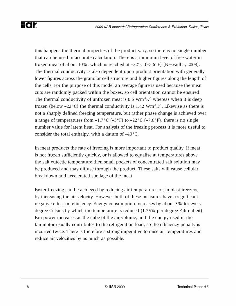
this happens the thermal properties of the product vary, so there is no single number

that can be used in accurate calculation. There is a minimum level of free water in

frozen meat of about 10%, which is reached at –22°C (–7.6°F) (Nesvadba, 2008).

The thermal conductivity is also dependent upon product orientation with generally

lower figures across the granular cell structure and higher figures along the length of

the cells. For the purpose of this model an average figure is used because the meat

cuts are randomly packed within the boxes, so cell orientation cannot be ensured.

The thermal conductivity of unfrozen meat is 0.5 Wm-1K-1 whereas when it is deep

frozen (below –22°C) the thermal conductivity is 1.42 Wm-1K-1. Likewise as there is

not a sharply defined freezing temperature, but rather phase change is achieved over

a range of temperatures from –1.7°C (–3°F) to –22°C (–7.6°F), there is no single

number value for latent heat. For analysis of the freezing process it is more useful to

consider the total enthalpy, with a datum of –40°C.

In meat products the rate of freezing is more important to product quality. If meat

is not frozen sufficiently quickly, or is allowed to equalise at temperatures above

the salt eutectic temperature then small pockets of concentrated salt solution may

be produced and may diffuse through the product. These salts will cause cellular

breakdown and accelerated spoilage of the meat

Faster freezing can be achieved by reducing air temperatures or, in blast freezers,

by increasing the air velocity. However both of these measures have a significant

negative effect on efficiency. Energy consumption increases by about 3% for every

degree Celsius by which the temperature is reduced (1.75% per degree Fahrenheit).

Fan power increases as the cube of the air volume, and the energy used in the

fan motor usually contributes to the refrigeration load, so the efficiency penalty is

incurred twice. There is therefore a strong imperative to raise air temperatures and

reduce air velocities by as much as possible.



Mathematical Modelling

Over the last hundred years, methods of calculating freezing times have become

increasingly complex in the pursuit of increased accuracy. A good overview of recent

model developments is given by Pham (2002). The more complex models can handle

a wide variety of shapes and products, and account for varying external conditions,

but they are generally difficult to follow without expert knowledge and often require

significant computing power or programming capability. The objective in developing

this model was to produce reasonable accuracy for simple geometries without using

expensive software and without any program writing, so it was decided to use a

spreadsheet for the model and display the result as a chart.

Freezing can be approximated by Plank’s equation, shown in equation 1, originally

developed in 1913. However this introduces some serious inaccuracies and can

result in over- or under-estimation by a factor of 30%. For example, the basic Plank

equation only considers the time from the onset of freezing (at temperature tf ) until

the latent heat, L, has been removed. It assumes that all the phase change takes place

at constant temperature, and that the ambient temperature, ta, remains constant

throughout the freezing process. It also assumes that the thermal conductivity is

constant throughout the freezing process. None of these assumptions is valid in real

applications.

=L

(tf – ta)

PD

h +

RD2

k (1)

where is the total time to achieve the require core temperature, L is the latent

heat, tf and ta are the temperatures of the product phase change and the surrounding

air respectively, h and k are the surface heat transfer coefficient and the thermal

conductivity respectively, D is a characteristic dimension of the product and P and

R are shape factors calculated from the block dimensions. A graph of these values



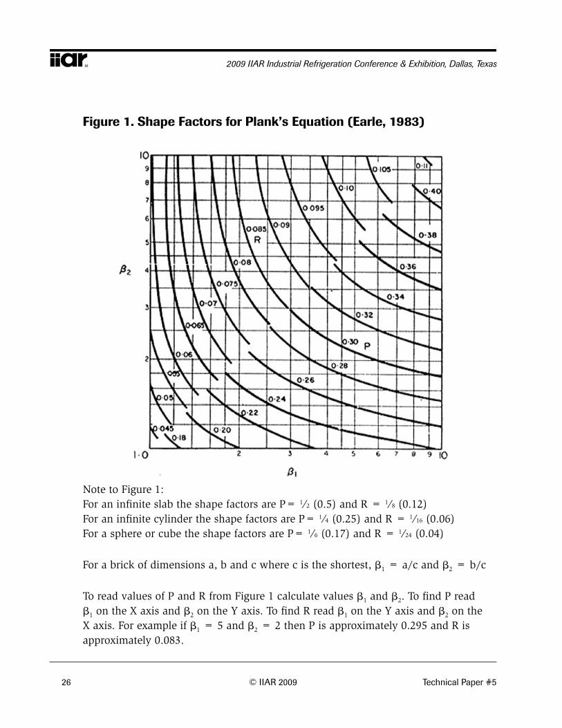
is shown in Figure 1, (Earle, 1983) where 1 and 2 are the ratios of the two longest

sides to the shortest. For the box dimensions given previously 1 and 2 are 4 and

2.6, so P and R are 0.307 and 0.086 respectively. With a latent heat of 230kJ kg-1 and

an assumed heat transfer coefficient of 20 Wm-2 K-1 the basic equation 7.22 hours as

the freezing time (Earle, 1983). A revised version of the Plank equation, developed by

Cleland and Earle (ASHRAE, 2006) using more complicated shape factors, is

=H18

(tf – ta)

PD

h +

RD2

k (2)

where H18 is the change in total enthalpy from the onset of freezing to –18°C (0°F).

It should be noted that these factors P and R are modified from the previous values

used in the simple Plank equation. With P and R calculated to be 0.447 and 0.224

respectively (using the method detailed in Chapter 10 of ASHRAE, 2006), with a

value of 271 600 kJ m-3 as H18 and with the surface heat transfer coefficient, h, again

taken to be 20 W m-2 K-1 the time to freeze the box to a core temperature of –18°C in

an air temperature of –36°C was calculated to be 15.89 hours. This correlates well

with site experience of a 16 hour cycle.

However, there are some serious flaws even with the revised version and it is likely

that the close agreement with site observations is the result of multiple errors tending

to cancel each other out. For example it is clearly not reasonable to assume that the

air temperature is –36°C at all times, nor that the thermal conductivity is constant

through the freezing process. Ultimately the accuracy of the calculation is dependent

upon the value of surface heat transfer coefficient which is assumed by the user,

and the calculated result can be matched to any observed value by changing the

assumptions used in the selection of the value for surface heat transfer coefficient.

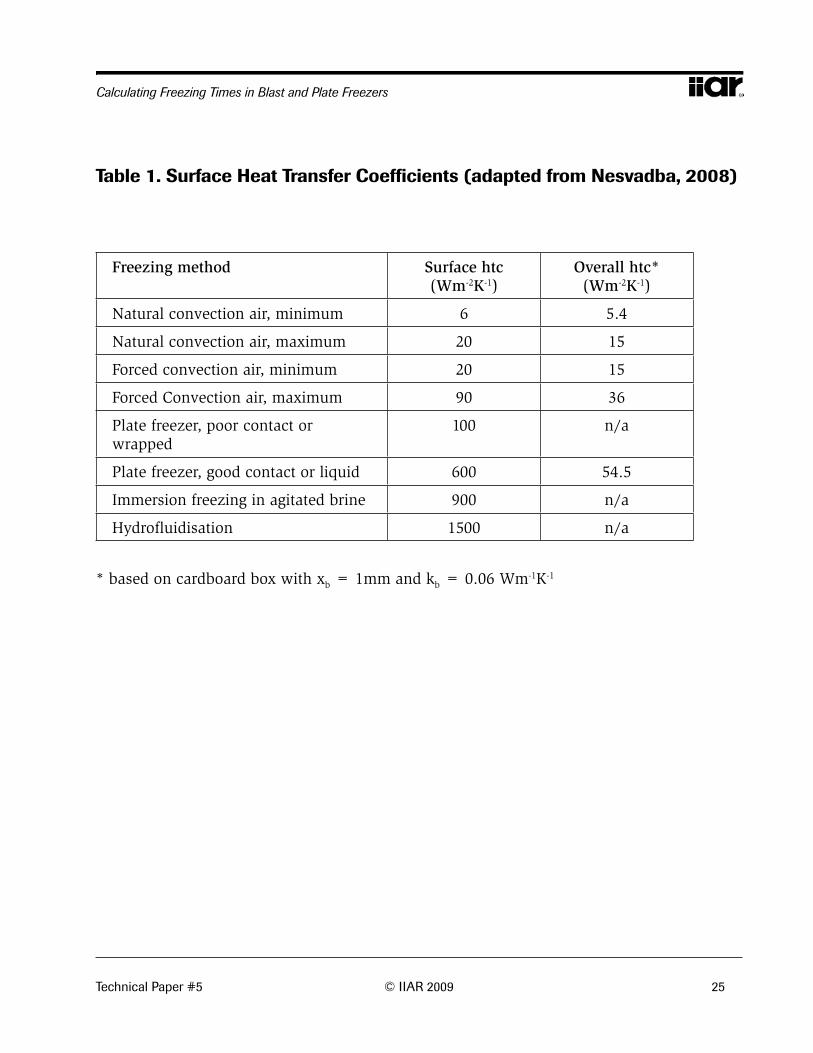
The surface heat transfer coefficient is primarily affected by the freezing process

used. Air in natural convection can achieve between 6 Wm–2K–1 and



20 Wm–2K–1, depending upon the temperature difference, surface roughness and

product orientation whereas blast freezers can provide coefficients from 20 Wm–2K–1

to 90 Wm–2K–1. Plate freezers achieve coefficients ranging from 100 Wm–2K–1

for badly wrapped or poorly positioned product to 600 Wm–2K-1 for liquids and

close contact solids. Freezing by immersion in brine gives even higher values, up to

900 Wm–2K–1 or even up to 1500 Wm–2K–1 for hydrofluidisation, the use of high

velocity brine jets within the immersion tank (Nesvadba, 2008). These values are

tabulated in Table 1, showing the basic value of surface heat transfer coefficient and

the effect of adding packaging in the form of a 1mm layer of cardboard.

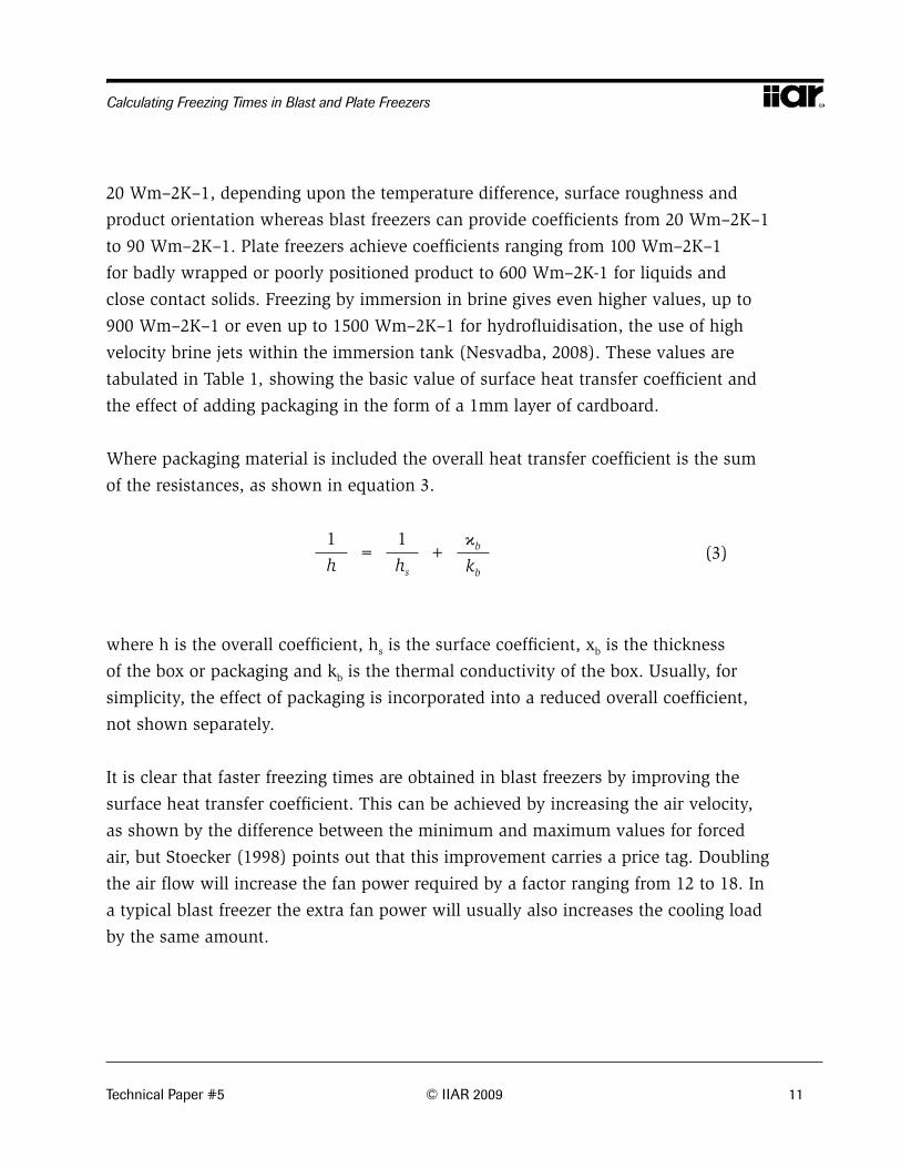
Where packaging material is included the overall heat transfer coefficient is the sum

of the resistances, as shown in equation 3.

1

h =

1

hs +

b

kb (3)

where h is the overall coefficient, hs is the surface coefficient, xb is the thickness

of the box or packaging and kb is the thermal conductivity of the box. Usually, for

simplicity, the effect of packaging is incorporated into a reduced overall coefficient,

not shown separately.

It is clear that faster freezing times are obtained in blast freezers by improving the

surface heat transfer coefficient. This can be achieved by increasing the air velocity,

as shown by the difference between the minimum and maximum values for forced

air, but Stoecker (1998) points out that this improvement carries a price tag. Doubling

the air flow will increase the fan power required by a factor ranging from 12 to 18. In

a typical blast freezer the extra fan power will usually also increases the cooling load

by the same amount.



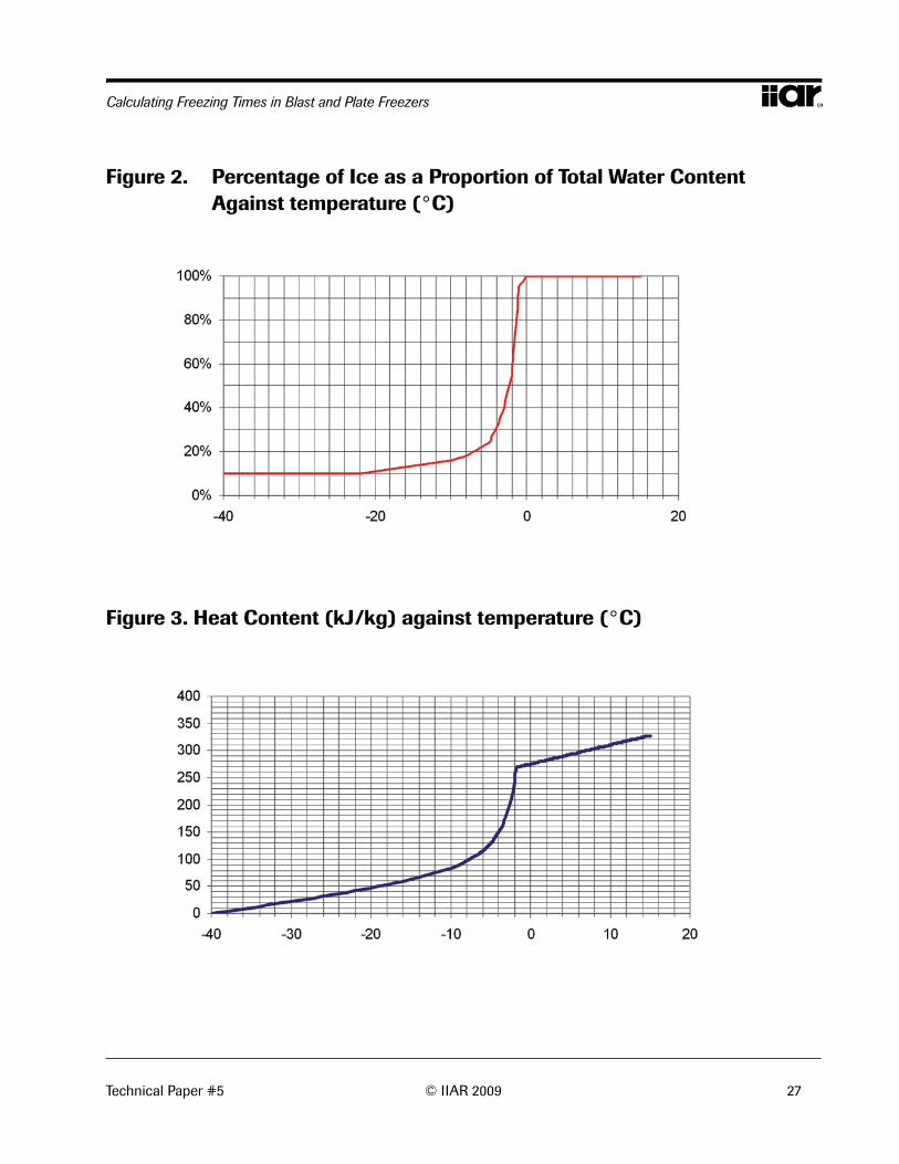
The ice content of the product is based upon data in Chapter 10 of the ASHRAE 2006

Refrigeration handbook. The ice content increases non-linearly from 0% at 0°C to

90% at –22°C as shown in Figure 2. The latent heat is modelled as variable specific

heat capacity with a step change from the value above freezing of 3.53 kJ kg-1 K-1 to

a peak value immediately below the onset of freezing of 76.4 kJ kg-1 K-1, reducing

asymptotically to the low temperature value of 2.13 kJ kg-1 K-1, shown in Figure 3. In

a similar way the thermal conductivity increases from 0.5 Wm-1K-1 when the product

is above freezing to 1.42 Wm-1K-1 when at low temperature as shown in Figure 4

(Pham, 2008).

To provide more accurate calculation of the behaviour of the product during the

freezing cycle, and to enable the use of variable enthalpy and thermal conductivity a

spreadsheet model for the freezing process was constructed. The spreadsheet is based

upon the Schmidt numerical method for assessing heating and cooling, but modified

to accommodate the change of state which progresses through the product as a

freezing front. The traditional Schmidt method divides the product into unit cells and

calculates the temperature of each cell at time ‘’ as the average of the temperatures

of the adjacent cells at time ‘ –1’. Special consideration is given to heat transfer at

the surface of the product where the temperature at time ‘’ is a combination of the

temperature of the adjacent block and the surrounding air temperature at time

‘ –1’. The relative importance of each of these is determined by the ratio of the heat

transfer by convection from the surface to the heat transfer through the product

by conduction. However to accommodate the thermal arrest during phase change

and the change of properties caused by the phase change the Schmidt method was

modified to consider total heat content rather than temperature. The enthalpy of each

cell was calculated by an averaging process analogous to the Schmidt method and

then the temperature of the cell was determined by correlation with the enthalpy

function described previously. This approach also allowed the values of specific

heat and thermal conductivity to be varied from cell to cell, which is not normally

possible in the Schmidt method. The key to successful application of the Schmidt

method is the selection of appropriate cell size and time interval to suit the product



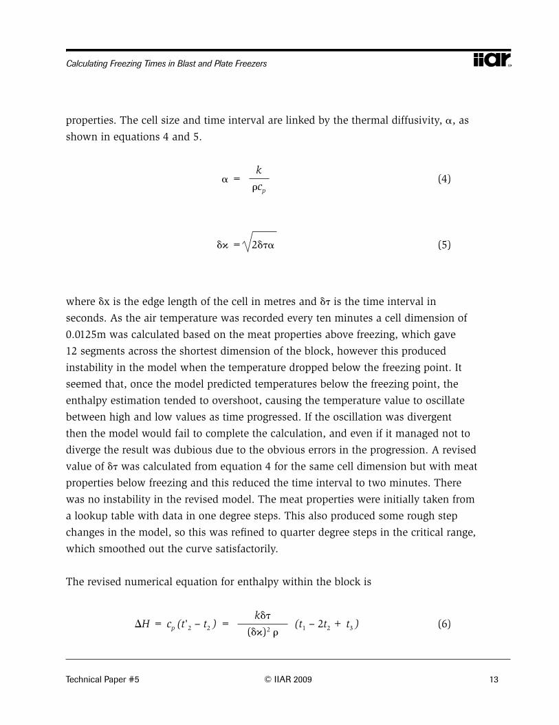
properties. The cell size and time interval are linked by the thermal diffusivity, , as

shown in equations 4 and 5.

=

k

cp (4)

=

(5) 2

where x is the edge length of the cell in metres and is the time interval in

seconds. As the air temperature was recorded every ten minutes a cell dimension of

0.0125m was calculated based on the meat properties above freezing, which gave

12 segments across the shortest dimension of the block, however this produced

instability in the model when the temperature dropped below the freezing point. It

seemed that, once the model predicted temperatures below the freezing point, the

enthalpy estimation tended to overshoot, causing the temperature value to oscillate

between high and low values as time progressed. If the oscillation was divergent

then the model would fail to complete the calculation, and even if it managed not to

diverge the result was dubious due to the obvious errors in the progression. A revised

value of was calculated from equation 4 for the same cell dimension but with meat

properties below freezing and this reduced the time interval to two minutes. There

was no instability in the revised model. The meat properties were initially taken from

a lookup table with data in one degree steps. This also produced some rough step

changes in the model, so this was refined to quarter degree steps in the critical range,

which smoothed out the curve satisfactorily.

The revised numerical equation for enthalpy within the block is

H = cp (t'2

– t2 ) =

k

()2 (t1

– 2t2 + t3 )

(6)



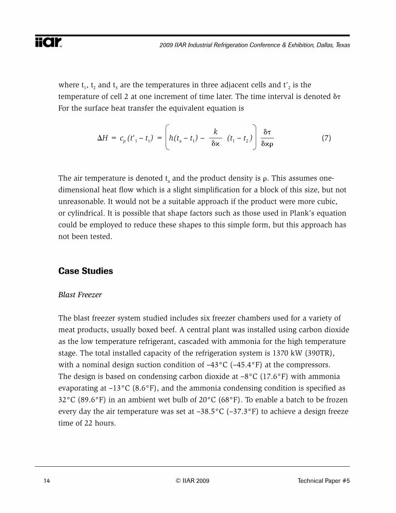
where t1, t2 and t3 are the temperatures in three adjacent cells and t’2 is the

temperature of cell 2 at one increment of time later. The time interval is denoted

For the surface heat transfer the equivalent equation is

H = cp (t'1

– t1) = h(ta

– t1) –

k

(t1

– t2 )

(7)

The air temperature is denoted ta and the product density is . This assumes one-

dimensional heat flow which is a slight simplification for a block of this size, but not

unreasonable. It would not be a suitable approach if the product were more cubic,

or cylindrical. It is possible that shape factors such as those used in Plank’s equation

could be employed to reduce these shapes to this simple form, but this approach has

not been tested.

Case Studies

Blast Freezer

The blast freezer system studied includes six freezer chambers used for a variety of

meat products, usually boxed beef. A central plant was installed using carbon dioxide

as the low temperature refrigerant, cascaded with ammonia for the high temperature

stage. The total installed capacity of the refrigeration system is 1370 kW (390TR),

with a nominal design suction condition of –43°C (–45.4°F) at the compressors.

The design is based on condensing carbon dioxide at –8°C (17.6°F) with ammonia

evaporating at –13°C (8.6°F), and the ammonia condensing condition is specified as

32°C (89.6°F) in an ambient wet bulb of 20°C (68°F). To enable a batch to be frozen

every day the air temperature was set at –38.5°C (–37.3°F) to achieve a design freeze

time of 22 hours.



Tests from site show that the product is sufficiently frozen typically after 16 hours,

although the blast freezer chambers are frequently overloaded by as much as 15%.

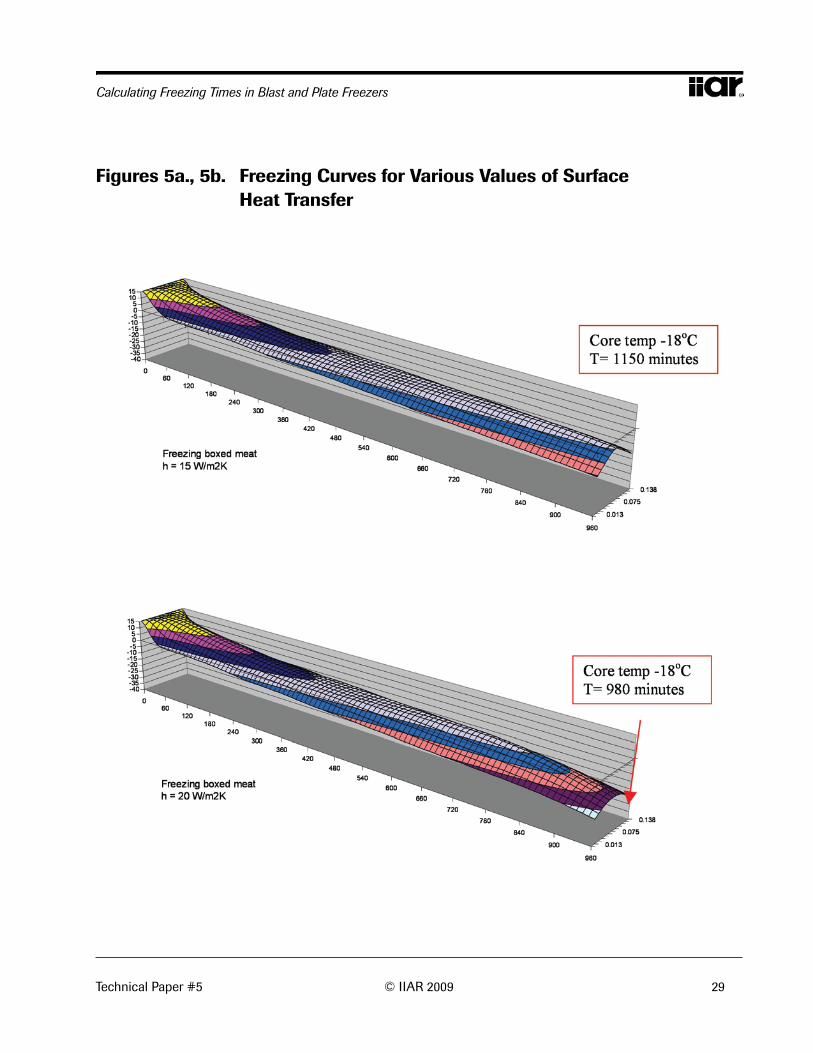
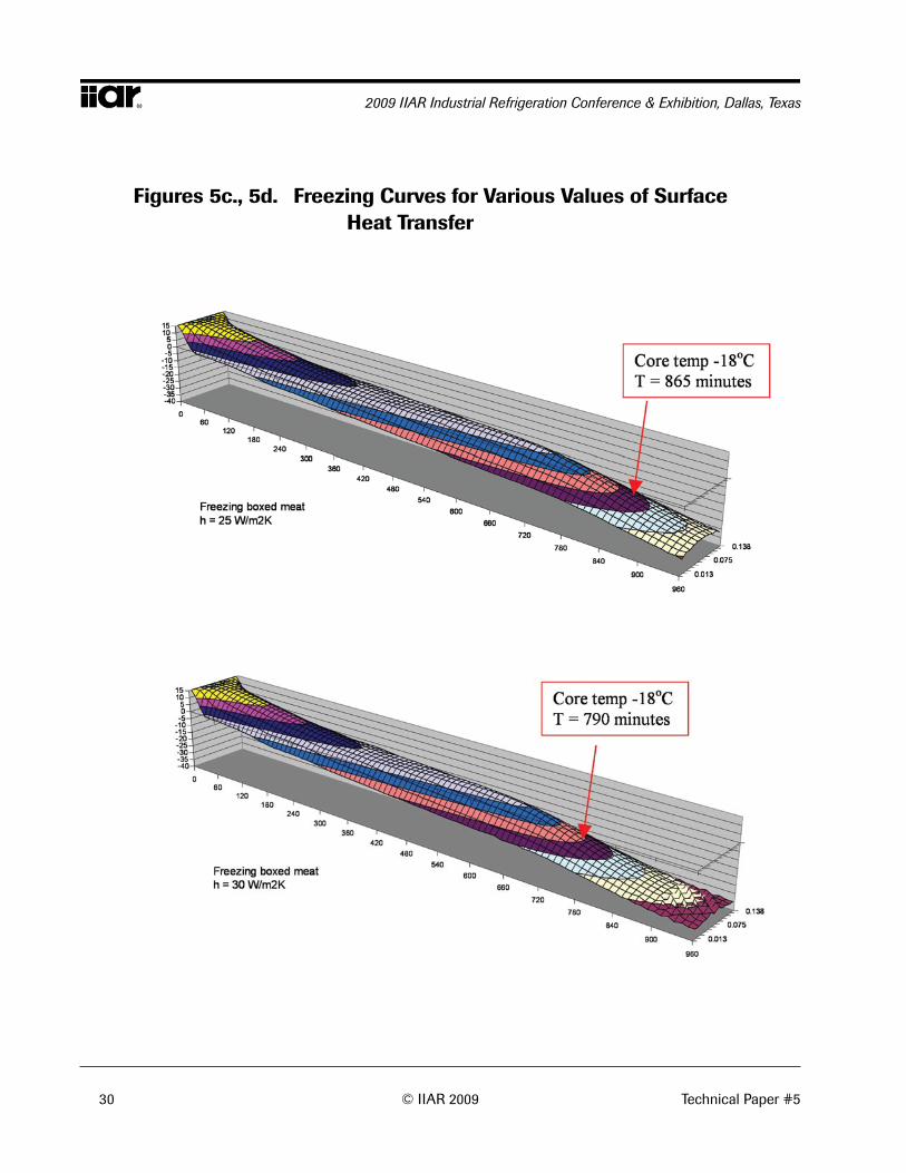
The spreadsheet model was used to investigate the relative importance of initial air

temperature pull down versus surface heat transfer performance. Figure 5 shows

four time-temperature charts for boxes of beef assuming various heat transfer

coefficients ranging from 15 Wm-2K-1 to 30 Wm-2K-1. For comparison a reduced rate of

air pulldown was modelled to simulate the performance of an ammonia evaporator,

assuming that the initial pull down is slower but that the air reaches the same

temperature as the carbon dioxide system after ten hours. On this basis there is very

little difference in the core temperature after 16 hours. With the more rapid start the

core reaches –18°C after 16:10 hours, with a surface htc of 20 Wm-2K-1 whereas with

the slower start it reaches –16.25°C and takes a further 20 minutes to get to –18°C.

In contrast the time taken to reach –18°C with a surface heat transfer coefficient of

15 Wm-2K-1 is 19:10 hours and with a value of 30 Wm-2K-1 it is only 13:10 hours.

Plate Freezer

The plate freezer system comprises 16 units each with 26 stations, giving a total

product load of 1000kg (2200 lbs) per unit. With a freeze cycle of two hours this gives

the capability to freeze 1000 tonnes of product per week on a five-and-a-half day

shift pattern. The installed capacity is 1000kW (286TR) at –50°C (–58°F) compressor

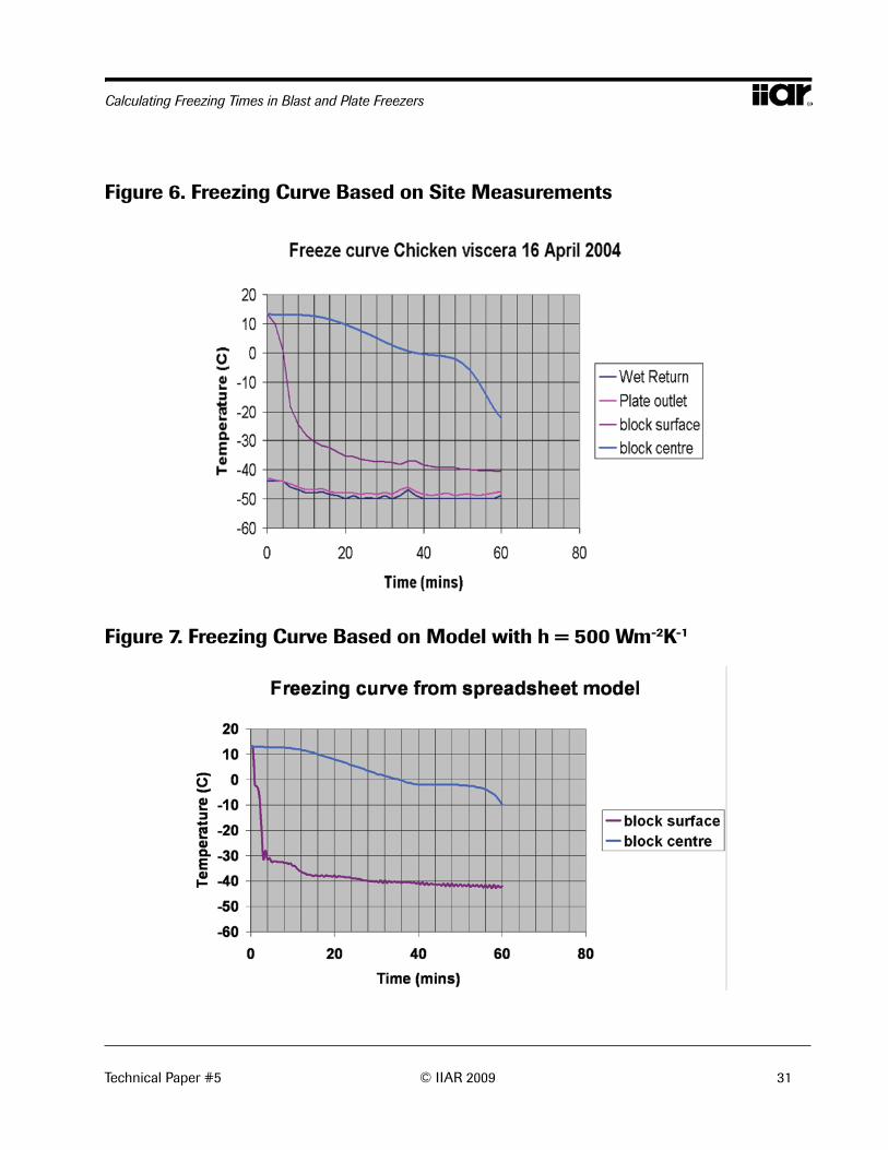
saturated suction temperature. Site freezing tests conducted in 2004 showed that the

time taken to achieve –18°C at the core was 58 minutes, as shown in Figure 6.

The model was reconfigured for plate freezer operation and various values of

heat transfer coefficient were tried. It was found that the model became unstable if

the heat transfer value were greater than 500 Wm-2K-1 as shown in Figure 7.

This is presumably because the look up table is not sufficiently fine, since the values

for , x and are not affected by surface heat transfer. A value of 600 Wm-2K-1

is suggested by Earle (1983) for unwrapped meat—it can be seen by comparison

of Figures 5 and 6 that this will give good agreement with the site measurements.

Further work is required in refinement of the model to allow this to be confirmed.



Conclusions

The changes in food properties during freezing are too great to allow simple

‘single number’ parameters to be used for estimating freezing times. In particular

the changes in specific heat capacity and thermal conductivity occur over a wide

temperature range, not at a single point, due to the manner in which the freezing

process progresses. Despite this inherent inaccuracy, simple methods such as Plank’s

equation are frequently used because they offer a quick answer. Plank’s equation can

always be adjusted to match empirical observations by adjusting the value used for

surface heat transfer coefficient. This makes it useful for comparing freezing times for

different products in the same process, but not so good for comparing processes or

the effects of adjusting external parameters such as air velocity or temperature.

The Schmidt method gives a structured form for calculating heat transfer through a

solid body and can be solved either arithmetically or graphically but it does not cope

well with phase change during heat transfer, nor with changes in food properties.

To model the freezing process, a modified version of the Schmidt method was used,

based on enthalpy rather than temperature and using look up tables for ice content,

enthalpy and thermal conductivity. The specific heat capacity for a given temperature

is the rate of change of enthalpy with respect to temperature. The time interval and

cell size used in the Schmidt method are both dependent on the food properties. If

incorrect values are used for the time step or the cell size then the model is likely to

be unstable. This shows up in the results as wild swings in temperature which clearly

could not happen in practice, and generally indicates that the time interval is too

large, causing temperature estimates to overshoot. The properties of the food in the

fully frozen state should be used to establish a suitable cell size and time interval.

This method is particularly well suited to modelling in a spreadsheet provided the

product shape allows one-dimensional heat transfer to be assumed. This is possible

with slabs of product, as in a plate freezer or with flat boxes, but the method does

not suit spheres, cylinders or cubes. It might be possible to develop the model



further using shape factors. This is probably simpler, if two or three dimensional

modelling is required, rather than attempting to add dimensions to the spreadsheet.

The advantages of modelling in a spreadsheet are that the freezing process can be

visualised easily and changes in key parameters can be investigated quickly.

In simulations of blast freezing and plate freezing, the spreadsheet model showed

good agreement with site measurements, although some further refinement is

required for plate freezers.

In this manner, the excellent results achieved in a blast freezer using carbon dioxide

as the refrigerant were investigated. It had been suggested that faster freezing

times were achieved because the evaporators were better able to cope with extreme

overload at the start of the freezing process. However, the freezing model suggests

that the time taken to achieve core temperature is still much more sensitive to the

surface heat transfer coefficient, particularly in the latter stages of freezing, than it is

to the initial air temperature pulldown.

The plate freezer model, although not able to cope with the very high heat transfer

coefficient expected in practice, suggests that the extraordinary improvement in

freezing time compared to previous experience on ammonia systems is largely due to

the properties of carbon dioxide and particularly to the relatively small effect which

pressure drop has on saturation temperature.

Acknowledgements

The author would like to thank the directors and staff of Star Refrigeration for

supporting this work and for permission to publish the results. Thanks are also due

to Dr. Sandy Small for his assistance in refining the model and providing guidance

for further improvements, and to the staff of Prosper de Mulder, Doncaster, England

and Granville Food Care, Dungannon, N. Ireland for the results reported in the case

studies.



Nomenclature

Symbol Description, units Symbol Description, units Time to freeze, s 1 Ratio of longest to shortest side, –

L Latent Heat, kJkg-1 2 Ratio of middle to shortest side, –

tf Freezing point, °C H18 Enthalpy change from 0°C to –18°C

ta Air temperature, °C Elapsed time in freezing calculation, s

P Shape factor, – Thermal diffusivity, m2s-1

R Shape factor, – Time interval, s

D Characteristic dimension, m H Enthalpy change, kJkg-1

h Overall heat transfer coeff, Wm-2K-1

cp Specific heat capacity, kJkg-1K-1

k Thermal conductivity,Wm-1K-1 Density, kg m-3

x Distance through block, m x Size of computation cell, m

hs Surface heat transfer coeff, Wm-2K-1

kb Thermal conductivity of box,Wm-1K-1

xb Thickness of box, m



References

ASHRAE, Refrigeration Handbook Chapter 10, Cooling and Freezing Times of Food,

Atlanta, 2006

Earle, R.L., Unit operations in food processing, chapter 6—Second ed. Pergamon Press, 1983

Hrnjak, P. and Park, C., In-Tube Heat Transfer and Pressure Drop Characteristics Of Pure

NH3 And CO2 In Refrigeration Systems, Proc IIR Conference, Ohrid, 2007

Nesvadba, P., Thermal Properties and Ice Crystal Development in Frozen Food, in Frozen

Food Science and Technology, Evans, J., ed, Blackwell, Oxford, 2008

Pearson, A., Evaporator performance in Industrial CO2 systems, International Institute

of Ammonia Refrigeration Annual Meeting, Acapulco, 2005

Pearson, A., A multi-chamber blast freezer with carbon dioxide as refrigerant, Proc IIR

Conf, Copenhagen, 2008

Pham, Q., Calculation of Processing Time and Heat Load During Food Refrigeration,

Proc AIRAH Conf, Sydney, 2002

Pham, Q., Modelling of Freezing Processes, in Frozen Food Science and Technology,

Evans, J., ed, Blackwell, Oxford, 2008

Stoecker, W., Industrial Refrigeration Handbook, p. 573, McGraw-Hill, 1998

Stoecker, W., Ammonia/Carbon Dioxide Hybrid Systems: Advantages and Disadvantages

International Institute of Ammonia Refrigeration, Annual Meeting, Nashville, 2000

UNEP, 2006 Assessment Report of the Refrigeration, AC and Heat Pumps Technical

Options Committee, UNEP Nairobi, February 2007



Appendix 1. Modelling in a Spreadsheet

The one-dimensional freezing process is well suited to modelling in a spreadsheet

because an individual worksheet can contain the one dimension of length plus time

as a second dimension and the resultant temperature profile with time can be easily

visualised in a three-dimensional chart (Figure 5). If two-dimensional modelling

were required then an additional worksheet for each second dimension slice would

be required and the process would become unwieldy. The graphical representation

would also be difficult, and would be best handled by producing a three-dimensional

chart for each one dimensional slice of the product that was of interest. In practice,

because the core temperature at the centre of the block is usually the only point

of interest in a freezing problem it is sufficient to model one dimension on the

centreline of the product, with suitable adjustment factors for shape. The problem of

two or three dimensional modelling is better handled in a computer program using

three or four dimensional matrices but concise presentation of the results would be

very complicated.

The model was created in Microsoft® Excel 2003. Any similar spreadsheet software

will have equivalent functionality. The spreadsheet includes some basic properties of

the product, including density above and below freezing, thermal conductivity and

specific heat. The thermal conductivity and specific heat are used to produce a look

up table based upon a correlation of temperature against unfrozen water content,

(Figure 2).

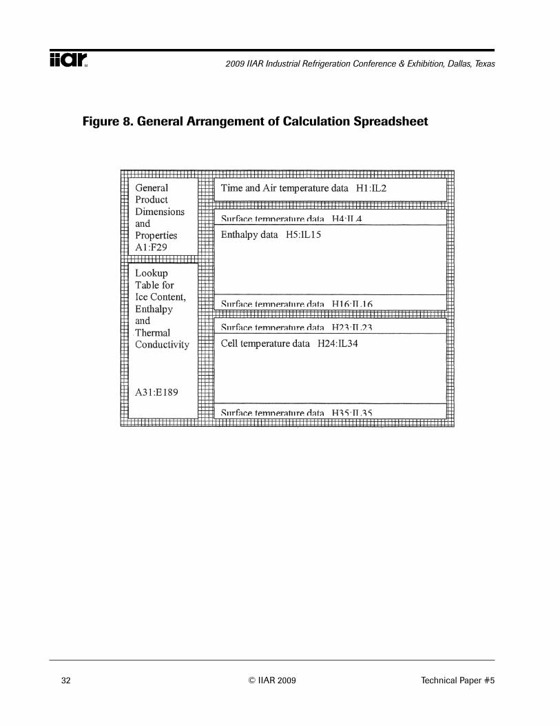
The general layout of the sheet is shown in Figure 8.

The calculation is done in two ranges, one for enthalpy (rows 5 to 15) and a

corresponding one for temperature (rows 24 to 34). The basic product parameters

are contained in columns A to E, with the first time cell (T=0) in column I. Each

column to the right of I represents a further time increment. The basic methodology

is to calculate the enthalpy of each cell based on the conditions of the adjacent cells



in the previous time period (to the left) and then to use the lookup table to calculate

the temperature corresponding to that heat content. The basic equations used in

the spreadsheet are given in equations 5 and 6 in the paper for internal and surface

cells respectively. For example the enthalpy for cell J5 (the surface cell after one time

increment) is represented in the spreadsheet by the terms

=I5+(($C$5*$C$1*((I23+J23)/2-I24)-VLOOKUP(I24,$C$32:$E$189,3)*(I24-I25))*

(J$1-I$1)*60/($C$1^2*IF(I24<0,$C$6,$E$6)*1000))

and likewise the enthalpy of the corresponding cell below the surface, J6, is calculated as

=I6+(VLOOKUP(I25,$C$32:$E$189,3)*(J$1-I$1)*60/($C$1^2*IF(I25<0,$C$6,$E$6)*1000)*

(I24-(2*I25)+I26))

In these expressions the term VLOOKUP(I25,C32:E189,3) reads the thermal conductivity

at temperature given in cell I25 from the range in cells C32 to E189 (the look up table

of properties). The IF( ) clause allows different values of density to be used above and

below freezing and the term (J1–I1)*60 gives the time interval in seconds. Note that the

dollar signs are used to fix the row or column of a cell reference, enabling the formula

to be copied to multiple cells without changing the reference, for example for the basic

parameters or the look up table.

The temperature of each cell is derived by using the calculated enthalpy values in the

lookup table. The expression for cell J24 is =VLOOKUP(J5,B32:C189,2). It would be

possible to have a function for temperature expressed as enthalpy, but this would be

a different polynomial for each product modelled, and would make automating the

spreadsheet more difficult (see Appendix 2).



When the model was based on a 10-minute interval it fitted onto a single worksheet,

which is 256 cells wide. However cutting the interval to 2 minutes increased the

width of range required, which meant that the full range had to be spread over three

sheets.

If starting afresh it would be better to orient the range vertically in order to progress

from top to bottom rather than left to right—the standard Excel sheet has 65,536

rows but only 256 columns. If the sheet is changed then the command for the lookup

table would become HLOOKUP.



Appendix 2. Automating the Spreadsheet

The basic model can be extended by using the built in macro program language in

Excel, Visual Basic. The Visual Basic editor is accessed by pressing <ALT> F11

when the spreadsheet is open.

Visual Basic is different from more traditional programming languages (BASIC,

FORTRAN, etc.) because it is event-based. When a macro is live it runs in the

background and responds to specific events such as keystrokes or soft-buttons

(control graphics superimposed onto the computer screen) to run associated

subroutines. These subroutines comprise a combination of standard Excel

functions and logic statements to determine alternate courses of action. Using these

subroutines it is possible to open data files, manipulate information and write files

to disk. It is also useful in many cases to temporarily disable the spreadsheet screen

update, as this causes severe screen flicker in complex calculations and significantly

slows the process down.

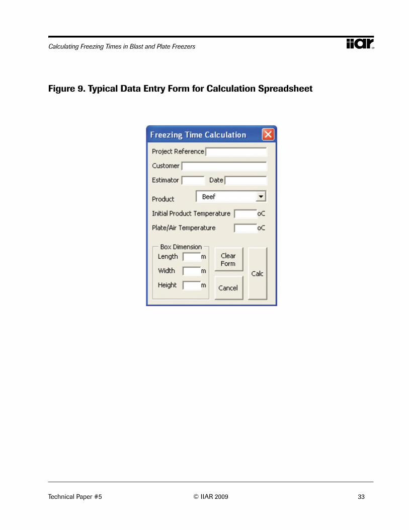
The benefit of adding macros to the freezing model is that it allows the user to build

up a library of product data and then specify product and conditions for a particular

case. Visual Basic allows the programmer to create a data input form with function

buttons, drop down menus, text boxes and other input devices (check boxes, toggle

buttons, option buttons, scroll bars, spin buttons, etc.). The form is used to enter

project data (Project Name, Reference Number, Date, User Initials), product data

(type of product, size of package, material of container) and performance data (air

velocity, refrigerant temperature, initial product temperature). At the end of the

calculation session the user has the opportunity to save the spreadsheet to a filename

compiled from the project details and the date. The user form should also include a

control button to calculate the new freezing time, one to reuse the previous inputs

and one to cancel the user input. The macro can be arranged to load automatically

when the spreadsheet is opened, but it is also useful to add a soft button to the

spreadsheet or specify a control key to run the form and call up the input form. It is



useful to have the spreadsheet open to an introduction page with notes on how to

use it if it will be available to people who are less familiar with the way it operates.

A typical data input form is shown in Figure 9.

The data form only allows for the final coolant temperature to be entered. For a

plate freezer this will be the plate surface, which will be almost the same as the

temperature of the refrigerant evaporating in the plates, and which will be nearly

constant throughout the freezing process. It must be remembered however that this

temperature might be substantially higher than the saturated temperature in the wet

suction header, due to pressure loss in the connecting hoses. For an air blast freezer

the assumption that the coolant temperature is constant is less reasonable. In this

case the macro for selecting the product type should be run once and then cancelled,

leaving a spreadsheet which can be modified to suit actual air temperature profiles if

they have been measured or estimated.

Where data for more than one product has been entered each product should be on

a separate worksheet. When the product is selected in the input form the macro will

switch to the appropriate sheet, copy the range containing the relevant data, switch

back to the calculation worksheet and paste the data into the appropriate position.



Table 1. Surface Heat Transfer Coefficients (adapted from Nesvadba, 2008)

Freezing method Surface htc(Wm-2K-1)

Overall htc*(Wm-2K-1)

Natural convection air, minimum 6 5.4

Natural convection air, maximum 20 15

Forced convection air, minimum 20 15

Forced Convection air, maximum 90 36

Plate freezer, poor contact or wrapped

100 n/a

Plate freezer, good contact or liquid 600 54.5

Immersion freezing in agitated brine 900 n/a

Hydrofluidisation 1500 n/a

* based on cardboard box with xb = 1mm and kb = 0.06 Wm-1K-1



Figure 1. Shape Factors for Plank’s Equation (Earle, 1983)

Note to Figure 1: For an infinite slab the shape factors are P= 1⁄2 (0.5) and R = 1⁄8 (0.12) For an infinite cylinder the shape factors are P= 1⁄4 (0.25) and R = 1⁄16 (0.06) For a sphere or cube the shape factors are P= 1⁄6 (0.17) and R = 1⁄24 (0.04)

For a brick of dimensions a, b and c where c is the shortest, 1 = a/c and 2 = b/c

To read values of P and R from Figure 1 calculate values 1 and 2. To find P read 1 on the X axis and 2 on the Y axis. To find R read 1 on the Y axis and 2 on the X axis. For example if 1 = 5 and 2 = 2 then P is approximately 0.295 and R is approximately 0.083.



Figure 2. Percentage of Ice as a Proportion of Total Water Content Against temperature (°C)

Figure 3. Heat Content (kJ/kg) against temperature (°C)



Figure 4. Thermal Conductivity (W/m2K) Against Temperature (°C)



Figures 5a., 5b. Freezing Curves for Various Values of Surface Heat Transfer



Figures 5c., 5d. Freezing Curves for Various Values of Surface Heat Transfer



Figure 6. Freezing Curve Based on Site Measurements

Figure 7. Freezing Curve Based on Model with h = 500 Wm-2K-1



Figure 8. General Arrangement of Calculation Spreadsheet



Figure 9. Typical Data Entry Form for Calculation Spreadsheet

Notes:



Documents

Tehcnical Paper: Calculating Freezing Times in Blast and Plate Freezers by Dr. Andy Pearson