Embed Size (px)
Citation preview
Technological Leadershipand Endogenous Growth
Susanto Basu∗, James Feyrer,†
& David Weil‡
First Draft: July 1998This Draft: February 8, 2002
Abstract
This paper investigates the interaction between technological leadershipand spillovers through a theoretical model where technological followers ben-efit from spillovers from a technological leader. Simulations of the model showthat technological leadership is persistent and history dependent. A more pa-tient nation may choose to remain behind an impatient technological leaderin order to benefit from spillovers. The result is lower steady state growththan would occur if the more patient nation took leadership. The probabilityof a persistent, impatient leader is higher the more easily technology flowsbetween nations.
Introduction
A typical feature of endogenous growth models is that the rate of growth is a function
of the discount rate.1 Countries with lower discount rates are more patient and invest
more in developing new technologies. The higher investment rate is rewarded with
more rapid technological progress and higher long run growth rates. If taken at face
value, models of this type predict that the income gap between two countries with
different discount rates will grow over time.
∗Department of Economics, University of Michigan†Department of Economics, Dartmouth College. E-mail : [email protected]‡Department of Economics, Brown University. E-mail : david [email protected] need to add some citations. Aghion and Howitt (1992), Romer (1986), Grossman and
Helpman (1991)
1
However, as noted by Gerschenkron (1962), Nelson and Phelps (1966) and oth-
ers2, technological growth need not be solely through the creation of new technolo-
gies as implied by the endogenous growth literature. Due to the non-rivalry of ideas,
the presence of technological spillovers allows a less technologically advanced nation
to grow in the absence of any domestically created technological advances.
It seems reasonable to think that the rate of technological spillovers will be a
function of the distance from the technological frontier. Countries far from the
frontier will have a large backlog of technologies to adopt, and will naturally choose
to adopt those technologies that have a high rate of return.3 As they near the
frontier, however, the number of technologies available for adoption will diminish
and the difference between adaptation and creation of new technologies will blur.
In the steady state, any country investing less in new technologies than the leader
will lag behind. Indeed, for any given level of investment in technology, there will
be a unique position below the technological frontier.
If the technological leader is also the most patient country in the world, it seems
clear that this is a stable arrangement. The rest of the countries in the world will
be impatient relative to the leader and will therefore want to invest less on new
technologies than the leader, even in autarky. As followers, these countries will
grow more rapidly than they would in autarky, while investing less on developing
new technologies.
What happens in the case when the technological leader is not the most patient
nation is less clear. Suppose that a relatively impatient nation is put in the position
of technological leader by historical accident and that a more patient nation is
in the following role. Are there any conditions under which this can be a stable
relationship?
The more patient nation is faced with a choice: invest less in technology, grow
more slowly than if alone in the world, and take advantage of technological spillovers;
or invest more in technology, grow at the autarky rate, and provide spillovers to the
follower. This tradeoff turns out to be consequential. If a less patient nation is the
technological leader in equilibrium, the world as a whole grows less rapidly. This
2Several papers in the endogenous growth literature have explicit models of spillovers, includingGrossman and Helpman (1991), Basu and Weil (1998) and Howitt (2000)
3Potential growth rates seem to be higher for countries away from the technological frontier.Evidence for this is the lack of examples of wealthy nations (presumably near the frontier) withsustained growth rates of greater than about 4%. On the other hand, there are several examplesof backward nations sustaining growth rates of nearly 10% for decades.
2
paper will examine the nature of this tradeoff and see when the more patient nation
chooses to follow and when they choose to lead.
The paper will describe the leadership choice in stages. Section one introduces
the model and describes the nature of balanced growth paths for exogenous levels
of investment in technological development. Section 2 endogenizes the choice of
technology investment and determines the optimal long run level of investment for a
leader and a follower. Given these optimal levels of investment, Section 3 describes
the balanced growth paths that are candidates to be equilibria in the long run.
Section 4 will then evaluate which of the possible balanced growth paths is a Nash
equilibrium.
1 The Model
The model is based on the basic model from Lucas (1988), simplified by using
log utility and neglecting population growth and capital depreciation. Endogenous
growth is produced through constant returns to accumulable factors and the steady
state growth rate is a decreasing function of the discount rate.4 Preferences over
per-capita consumption streams in country i are given by
Ui =∫ ∞
0eθit ln[ci(t)]dt (1)
Output is determined by a constant returns to scale Cobb-Douglas production
function two factors of production, physical capital and human capital augmented
labor. Labor can be allocated to production or to the accumulation of human
capital. Output per capita in country i is 5
4This model was chosen for simplicity. Models with more explicit microfoundations for in-novation such as Aghion and Howitt (1992) and Grossman and Helpman (1991) have a similarrelationship between the discount rate and the long run level of growth. This is the feature ofendogenous growth models that we wish to exploit.
5Throughout the paper, we are analyzing the solution to the social planner’s problem. Theresults of the paper continue to hold in a decentralized model with individual agents. In particular,the results hold if we introduce a composite human capital measure that allows spillovers betweenindividuals and the aggregate economy. The production function has the form
yi,j(t) = Bki(t)α[ui,j(t)hi,j(t)ψhi(t)1−ψ]1−α
where individual j’s proportion of labor used in production is ui,j(t) ∈ [0, 1] and individual j’slevel of physical capital is ki,j(t). The effective level of human capital for individual j in countryi is a constant returns to scale combination of the individual’s level of human capital, hi,j(t) and
3

yi(t) = Bki(t)α[ui(t)hi(t)]
1−α (2)
To further simplify the analysis, the marginal product of capital is set by an
exogenous interest rate. This allows us to express output without physical capital.
Removing capital does not qualitatively affect the results.
yi(t) = Aui(t)hi(t), A = B(
αB
r
) 11−α
(3)
The proportion of output not paid to physical capital is consumed each period.
We assume that capital flows across borders to equalize the marginal product of
capital but that international borrowing for consumption smoothing is not possible.
We further assume that the discount rate is higher than the world interest rate,
θi < r, ∀i. Under this condition, nations will want to borrow, so that the liquidity
constraint will be binding. The proportion of labor not used for producing output,
(1− ui), is used to produce human capital.
At any given time, the country with the highest level of human capital is the
technological leader. Let L be the subscript for the nation with the highest level
of human capital. The leader’s accumulation of human capital is unaffected by the
actions of follower countries. The form of the human capital accumulation equation
for the leader is based on the single country model of Lucas (1988)
hL(t) = [1− uL(t)] φhL(t), hL(t) ≥ hi(t) ∀i (4)
At any given time, nations with a lower level of human capital than the leader
are followers. In addition to domestically produced human capital, followers benefit
from spillovers from the human capital of the leader. For a follower, the size of
the spillover is a function of the level of human capital relative to the technological
leader. The larger the difference between the two, the larger the return to investment
in human capital. In other words, the farther a follower is behind the leader, the
larger the spillover.
hi(t) = [1− ui(t)] {φhi(t) + β [hL(t)− hi(t)]} , (5)
the average level of human capital within country i, hi(t) . As with physical capital in the Romer(1986) model, there is a spillover from human capital so that social returns to human capital arelarger than individual returns to human capital.
4
hi(t) < hL(t)
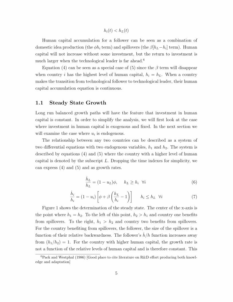
Human capital accumulation for a follower can be seen as a combination of
domestic idea production (the φhi term) and spillovers (the β[hL−hi] term). Human
capital will not increase without some investment, but the return to investment is
much larger when the technological leader is far ahead.6
Equation (4) can be seen as a special case of (5) since the β term will disappear
when country i has the highest level of human capital, hi = hL. When a country
makes the transition from technological follower to technological leader, their human
capital accumulation equation is continuous.
1.1 Steady State Growth
Long run balanced growth paths will have the feature that investment in human
capital is constant. In order to simplify the analysis, we will first look at the case
where investment in human capital is exogenous and fixed. In the next section we
will examine the case where ui is endogenous.
The relationship between any two countries can be described as a system of
two differential equations with two endogenous variables, h1 and h2. The system is
described by equations (4) and (5) where the country with a higher level of human
capital is denoted by the subscript L. Dropping the time indexes for simplicity, we
can express (4) and (5) and as growth rates.
hL
hL
= (1− uL)φ, hL ≥ hi ∀i (6)
hi
hi
= (1− ui)
[φ + β
(hL
hi
− 1
)]hi ≤ hL ∀i (7)
Figure 1 shows the determination of the steady state. The center of the x-axis is
the point where h1 = h2. To the left of this point, h2 > h1 and country one benefits
from spillovers. To the right, h1 > h2 and country two benefits from spillovers.
For the country benefiting from spillovers, the follower, the size of the spillover is a
function of their relative backwardness. The follower’s h/h function increases away
from (h1/h2) = 1. For the country with higher human capital, the growth rate is
not a function of the relative levels of human capital and is therefore constant. This
6Pack and Westphal (1986) [Good place to cite literature on R&D effort producing both knowl-edge and adaptation]
5

Figure 1: Steady State between Two Countries
0.50 1.00 1.50
h1/h2
h gr
owth
rat
e
Country 1
Country 2
( )φ11
1 1 uh
h−=
�
( )φ22
2 1 uh
h−=
�
( ) ��
���
����
�
�−+−= 11
1
21
1
1
h
hu
h
h βφ�
( ) ��
���
����
�
�−+−= 11
2
12
2
2
h
hu
h
h βφ�
(h1/h2)*
is represented in Figure 1 by the horizontal segments. The steady state is the point
where h1 and h2 grow at the same rate. In Figure 1, this is the crossing point of the
two lines, (h1/h2)∗.
Whether the steady state is to the left or the right of the (h1/h2) = 1 is de-
termined by the relative levels of investment in human capital. Suppose that the
level of human capital is the same in both countries, (h1/h2) = 1. Neither country
benefits from spillovers so the country with higher investment in human capital will
have higher growth. For Figure 1, country one has higher investment in human
capital accumulation (1− u1) > (1− u2).
The leader will always be the nation with highest human capital investment.
Equating (6) and (7) gives the stable relative levels of human capital for a follower.
This will be referred to as the steady state level of backwardness.
(hL
hi
)∗= 1 +
(ui − uL)
(1− ui)
φ
β(8)
6

2 Endogenous Steady States
In this section we extend the analysis of the previous section by endogenizing the
level of investment in human capital. We begin by examining balanced growth
paths where the level of investment in human capital accumulation is constant.7
Through dynamic optimization we can determine the long run levels of human
capital accumulation that result from optimizing behavior.
Along a balanced growth path a country must either lead or follow. For each
of these long run outcomes, they must satisfy a set of first order conditions at all
times. For these first order conditions we can calculate the balanced growth level of
investment in human capital accumulation.
2.1 The Technological Leader
This section will examine the balanced growth level of investment in human capital
accumulation for a country which is the leader on the balanced path. The current
value Hamiltonian the country with the highest level of human capital (dropping
the time indexes for simplicity) is
HL = ln(AuLhL) + mL [(1− uL)φhL] , hL(t) ≥ hi(t) ∀i (9)
An optimal path must satisfy the following first order conditions,
∂HL
∂uL
=1
uL
−mLφhL = 0 (10)
mL = −∂HL
∂hL
+ mLθL = − 1
hL
−mLφ(1− uL) + mLθL (11)
We are interested in balanced growth paths where the long run investment in
human capital is constant. The leader’s balanced path can be solved without any
knowledge of the follower’s behavior. The two first order conditions, (10) and (11),
can be combined to solve for the growth rate of the costate variable mL,
mL
mL
= −φ + θL (12)
For uL to remain constant, equation (10) implies that mL and hL must have
7This is similar to the constant long run saving rate in the Cass-Ramsey model. In both cases,constancy of the choice variable is a consequence of transversality conditions.
7

growth rates of equal magnitude and opposite sign. With (12) this allows us to
solve for the steady state growth rate of human capital and output.
hL
hL
= −mL
mL
= φ− θL (13)
Plugging this result in to the leader’s human capital accumulation equation
(6) we can determine the steady state value of u∗L which satisfies the first order
conditions,
hL
hL
= (1− uL)φ = φ− θL
u∗L =θL
φ(14)
For a country which is the leader on a balanced growth path, optimization implies
that the level of human capital accumulation is described by (14). In our simplified
dynamic system (with no capital) the leading nation is always on the balanced
growth path without transitional dynamics.
2.2 Technological Followers
This section will examine the balanced growth level of investment in human capital
accumulation for a country which is a follower on the balanced path. The current
value Hamiltonian for an individual in the follower nation is,
Hi = ln(Auihi) + mi {(1− ui) [φhi + β (hL − hi)]} , (15)
hi(t) < hL(t) ∀i
An optimal path must satisfy the following first order conditions,
∂Hi
∂ui
=1
ui
−mi [φhi + β (hL − hi)] = 0 (16)
mi = −∂Hi
∂hi
+ miθi = − 1
hi
−mi(φ− β)(1− ui) + miθi (17)
Again, we are interested in balanced growth paths where the long run investment
in human capital is constant. From the preceding section we saw that a technological
8

leader chooses a constant growth rate of human capital which is independent of the
actions of a follower nation. From the point of view of a technological follower, this
growth rate is exogenous in a long run steady state. Let gL be the growth rate
chosen by the leader.
As before, we are considering long run steady states where the level of ui is
constant. In Section 1 we showed that there is a stable steady state between two
nations choosing constant levels of investment in human capital accumulation. In
this steady state, the ratio hL/hi is constant.
Using these two features of the steady state we can solve for the level of u∗i which
satisfies the first order conditions for a follower. The two first order conditions, (16)
and (17), can be combined to solve for the growth rate of the costate variable mi,
mi
mi
= −uiβhL
hi
− (φ− β) + θi (18)
If ui and the ratio hL/hi are to remain constant, (16) implies that mi and hi must
have growth rates of equal magnitude and opposite sign. The constancy of hL/hi
allows us to equate the growth rate of hi with the growth rate of hL determined in
the leader’s problem by equation (13).
mi
mi
= − hi
hi
= − hL
hL
= −gL (19)
Equating (18) and (19),
βhL
hi
=gL + θi
ui
+β − φ
ui
(20)
Using the follower’s human capital accumulation equation (7) we can determine
the optimum u∗i where the follower grows at the same rate as the leader along a
balanced growth path.
φ + βhL
hi
− β − uiφ− uiβhL
hi
+ uiβ = gL (21)
Using (20) to substitute out hL/hi terms,
φ +gL + θi
ui
+β − φ
ui
− β − uiφ− ui
(gL + θi
ui
+β − φ
ui
)+ uiβ = gL (22)
9

Rearranging and multiplying through by ui to get a quadratic equation in ui
[β − φ] u2i + [−2(β − φ)− 2gL − θi] ui + [β − φ + gL + θi] = 0 (23)
Solving for ui,8
u∗i =2(β − φ) + 2gL + θi −
√4gL(β − φ) + [2gL + θi]2
2(β − φ)(24)
Substituting in gL = φ(1− u∗L) from (6) we can express the steady state invest-
ment in human capital for a follower in terms of the steady state level investment
in human capital for the leader.
(1− u∗i ) =−2φ(1− u∗L)− θi −
√4φ(β − φ)(1− u∗L) + [2(1− u∗L) + θi]2
2(β − φ)(25)
Equation (25) describes the optimal choice of investment in human capital accu-
mulation along the balanced growth path for a follower as a function of the leader’s
investment in human capital. Assume that human capital in country i relative to
the leader is at the stable level defined by equation (8), h1/h2 = (h1/h2)∗, and that
ui(t) = u∗i ∀t. As long as the lead country grows at the rate gL, country i will satisfy
the first order conditions at all times. This is therefore the only optimal long run
choice if country i is a follower.
3 Optimal Long Run Equilibria
On a balanced growth path, each of the countries in our model must either lead or
follow. If they lead, they must satisfy the steady state optimality condition for a
leader, equation (14), and if they follow, they must satisfy the steady state optimality
condition for a follower, equation (25). Figure 2 shows both these possibilities for
country two in our model as a function of country one’s investment in human capital
accumulation, u1. The straight line, labelled “Lead,” is invariant to the level of u1
because if country two leads, their behavior is independent of country one. The
curved line, labelled “Follow,” shows the optimal long run response of country two
8only the positive root results in u∗i ∈ [0, 1]
10

to different levels of u1. These two lines represent the only possible choices of human
capital accumulation for country two along an optimal balanced growth path.
Figure 2: Optimal Responses for Country Two
0.0
0.1
0.2
0.3
0.4
0.5
0.6
0.7
0.8
0.9
1.0
0.0 0.1 0.2 0.3 0.4 0.5 0.6 0.7 0.8 0.9 1.0(1-u1)
(1-u
2)
Follow
Lead
A closer look at Figure 2 will show that portions of each line will not result in
a steady state as described in Section 1. Recall from Section 1 that the country
with the highest level of investment in human capital is always the leader in the
steady state. To the right of the 45o line, the Lead line indicates that country
two’s optimal level of investment in human capital as a leader is lower than country
one’s investment. Country two cannot lead if they invest less than country one in
human capital accumulation. Similarly, a portion of the Follow line lies above the
45o line. If country two’s optimal level of human capital accumulation as a follower
is larger than country one’s level, two cannot be a follower. Redrawing the graph to
include only the portions of each line which represent potential steady states results
in Figure 3.
If country one has low enough investment in human capital accumulation, coun-
try two has no choice but to lead in the long run. This is represented in Figure
3 by the region to the left of the grey rectangle. If country one has sufficiently
high human capital investment country two must follow on the balanced path (the
area to the right of the grey rectangle). In between the extremes, both leading and
following are possible long run equilibria. This is represented in Figure 3 by the
11
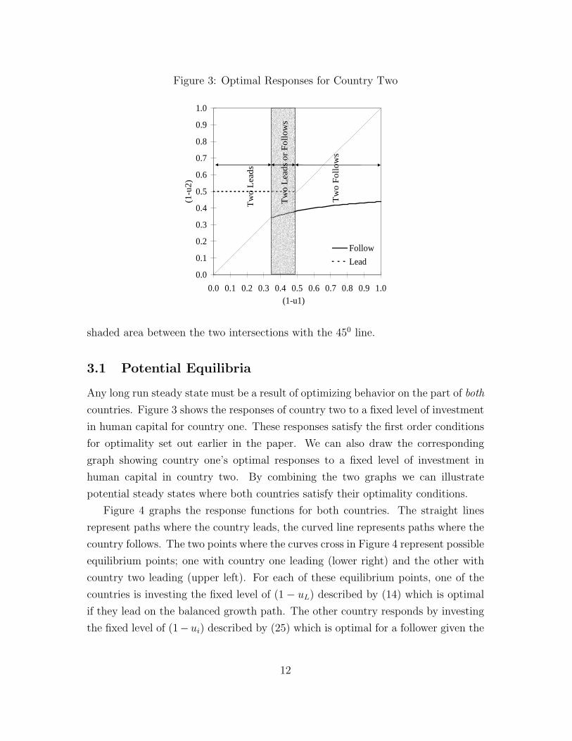
Figure 3: Optimal Responses for Country Two
0.0
0.1
0.2
0.3
0.4
0.5
0.6
0.7
0.8
0.9
1.0
0.0 0.1 0.2 0.3 0.4 0.5 0.6 0.7 0.8 0.9 1.0(1-u1)
(1-u
2)
Follow
Lead
Tw
o F
ollo
ws
Tw
o L
eads
Tw
o L
eads
or
Fol
low
s
shaded area between the two intersections with the 450 line.
3.1 Potential Equilibria
Any long run steady state must be a result of optimizing behavior on the part of both
countries. Figure 3 shows the responses of country two to a fixed level of investment
in human capital for country one. These responses satisfy the first order conditions
for optimality set out earlier in the paper. We can also draw the corresponding
graph showing country one’s optimal responses to a fixed level of investment in
human capital in country two. By combining the two graphs we can illustrate
potential steady states where both countries satisfy their optimality conditions.
Figure 4 graphs the response functions for both countries. The straight lines
represent paths where the country leads, the curved line represents paths where the
country follows. The two points where the curves cross in Figure 4 represent possible
equilibrium points; one with country one leading (lower right) and the other with
country two leading (upper left). For each of these equilibrium points, one of the
countries is investing the fixed level of (1− uL) described by (14) which is optimal
if they lead on the balanced growth path. The other country responds by investing
the fixed level of (1− ui) described by (25) which is optimal for a follower given the
12

Figure 4: Symmetric Response Functions - Two Possible Equilibria
0.0
0.1
0.2
0.3
0.4
0.5
0.6
0.7
0.8
0.9
1.0
0.0 0.1 0.2 0.3 0.4 0.5 0.6 0.7 0.8 0.9 1.0(1-u1)
(1-u
2)
C2
C1
leader’s behavior.
For different parameter values, there may be only one crossing point and only
one possible equilibrium. Figure 5 illustrates this possibility. In Figure 4 both
countries share the same discount rate. For Figure 5 country one’s discount rate
was increased. The increased discount rate results in lower optimal investment,
shifting country one’s response functions to the left. The equilibrium point where
one remains in the lead is eliminated.
For any given set of parameters β and φ, the existence of one or two potential
equilibria will be a function of the discount rates of the two countries. We are
interested in identifying the set of discount rates pairs where there are two potential
long run equilibria, as illustrated by the crossing points in Figure 4. These are the
conditions under which it is possible for a less patient country to lead in the long
run.
Suppose that country two has a lower discount rate than country one. For there
to be two crossing points, the optimal level of investment by country two as a follower
must be lower than country one’s autarky investment at some point to the right of
the 45o line. Since the optimal response of two is an increasing function of one’s
investment in human capital, it is the case that two’s lowest possible investment level
is found where their response curve crosses the 45o. This investment level can be
13

Figure 5: Only One Possible Equilibrium
0.0
0.1
0.2
0.3
0.4
0.5
0.6
0.7
0.8
0.9
1.0
0.0 0.1 0.2 0.3 0.4 0.5 0.6 0.7 0.8 0.9 1.0(1-u1)
(1-u
2)
C2
C1
solved by setting he follower’s optimal response, (25) equal to the leaders invesment
level, (1 − uL). Solving and simplifying we find that the minimum sustainable
investment for country two is
(1− ui) =φ− θi
β + φ(26)
The minimum possible level of investment is decreasing in the discount rate (less
patient nations are willing to invest less), and decreasing in the spillover parameter
β (larger spillovers induce less investment).9
It is impossible for two to be a follower if the leader is investing less than two’s
minimum in human capital accumulation. The condition where two can potentially
follow can therefore be stated as
(1− u∗F ) > (1− ui) (27)
This condition simply states that the leader must invest more than the follower’s
minimum investment to retain leadership. Plugging in (14) and (26) we can describe
the conditions needed for two potential equilibria in terms of the discount rates of
9Indeed, as β → 0 the minimum level of investment by country two approaches the autarkylevel.
14
the two countries and the exogenous parameters.
θL
φ<
β + θi
β + φ(28)
Again, it is worth noting the effect of changes to the spillover parameter. As long
as φ > θi increasing β will increase the allowable discount rate of the leader.10 In
other words, as spillovers increase, you can sustain a larger gap between the leader
and follower’s discount rates. As β → ∞, any gap between the discount rates is
sustainable as long as the leader has positive growth.11 As β → 0, no gap between
the two discount rates is sustainable and the more patient nation will always lead.
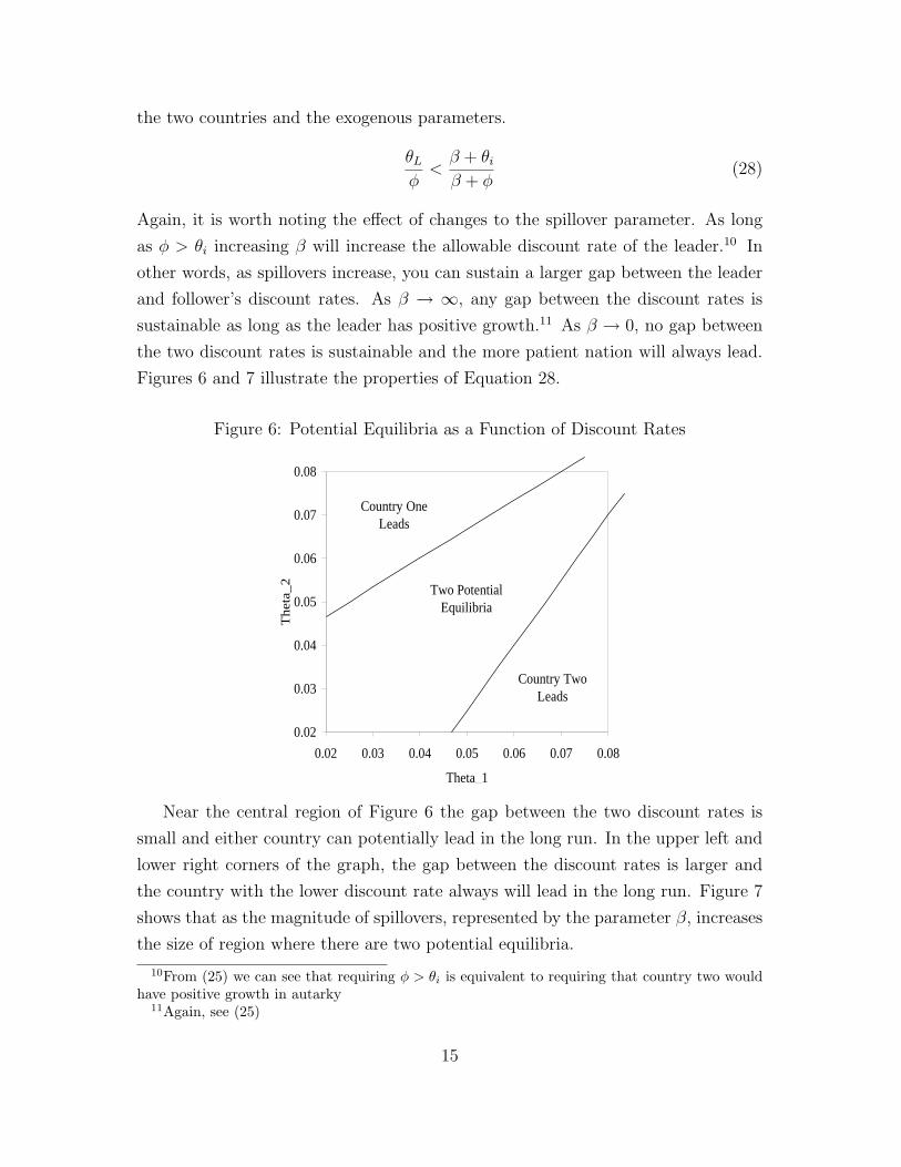
Figures 6 and 7 illustrate the properties of Equation 28.
Figure 6: Potential Equilibria as a Function of Discount Rates
0.02
0.03
0.04
0.05
0.06
0.07
0.08
0.02 0.03 0.04 0.05 0.06 0.07 0.08
Theta_1
Th
eta_
2
Two Potential Equilibria
Country One Leads
Country Two Leads
Near the central region of Figure 6 the gap between the two discount rates is
small and either country can potentially lead in the long run. In the upper left and
lower right corners of the graph, the gap between the discount rates is larger and
the country with the lower discount rate always will lead in the long run. Figure 7
shows that as the magnitude of spillovers, represented by the parameter β, increases
the size of region where there are two potential equilibria.
10From (25) we can see that requiring φ > θi is equivalent to requiring that country two wouldhave positive growth in autarky
11Again, see (25)
15

Figure 7: The Effect of Increasing Beta
0.02
0.03
0.04
0.05
0.06
0.07
0.08
0.02 0.03 0.04 0.05 0.06 0.07 0.08
Theta_1
Th
eta_
2Two Potential
Equilibria
Country One Leads
Country Two Leads
In the case where there are two potential equilibria (i.e., two crossing points
exist), these equilibria represent the only long run choices of investment in human
capital where both countries satisfy their respective first order conditions along
balanced growth paths. This does not imply, however, that both configurations are
optimal for both countries. It may be the case that one country will wish to deviate
from one of the long run paths in order to move to the other long run path. The
next section will describe the circumstances under which this is the case. In doing
so, we will be able to establish that one of the two potential balanced growth paths
is a Nash equilibrium.
At this point, we should note that the insights gained from analyzing the po-
tential long run equilibria continue to hold when we add transitional dynamics to
the analysis. Some of the potential equilibria described in the Figures 6 and 7 will
turn out to be unsustainable as Nash Equilibria, but the basic shape of the regions
remains intact. Long run paths where less patient nations are technological leaders
continue to be possible and the likelihood of this outcome increases with the rate of
technological spillovers.
16

4 Nash Equilibria
In this section we will examine the two potential equilibria described in the previous
section and determine the conditions under which these points are Nash equilibria.
Our discussion will encompass variation in three variables, the discount rates, θ1
and θ2, and the initial relative levels of human capital, h1(0)/h2(0).
In the long run, for any given set of parameters there are only two possible
configurations; country one leading and country two leading. For each of these
configurations, the long run investment in human capital accumulation and the
long run human capital ratio will be constant as determined in the previous section.
Given a set of discount rates and the initial human capital ratio, any optimal paths
of human capital accumulation must satisfy the differential equation system given
by the first order conditions, (10), (11), (16), and (17) at all points in time. The
problem is to find initial values for the control variables, u1(0) and u2(0), which put
each country on one of the two potential balanced growth paths.
There are two possible sets of initial conditions which lead to optimal balanced
growth paths given θ1, θ2 and h1(0)/h2(0):
[uL
1 (0), uF2 (0)
]
limt→∞uL
1 (t) = uL∗1 , lim
t→∞uF2 (t) = uF∗
2 , limt→∞
h1(t)
h2(t)=
(h1
h2
)∗> 1 (29)
[uF
1 (0), uL2 (0)
]
limt→∞uF
1 (t) = uF∗1 , lim
t→∞uL2 (t) = uL∗
2 , limt→∞
h1(t)
h2(t)=
(h1
h2
)∗< 1 (30)
where the superscripts L and F indicate the relative position of the country in the
steady state. If the two countries start with initial[uL
1 (0), uF2 (0)
]their optimal paths
will lead to country one leading and country two following along a balanced growth
path. As t gets large, each country’s investment in human capital accumulation will
approach the balanced growth levels described by equations (14) and (25). Similarly,
the human capital ratio approaches the steady state level of backwardness described
by (8).
For (29) country one leads along the balanced growth path; for (30) country two
leads along the balanced growth path. There is no reason to assume that both these
17

paths exist. As we showed in the last section, there are conditions under which only
one long run configuration is supportable in the long run.
Let
[uL1 (0..∞), uF
2 (0..∞)] (31)
[uF1 (0..∞), uL
2 (0..∞)] (32)
be the entire paths of u1(t) and u2(t) implied by (29) and (30). The paths (31) and
(32) are the only possible Nash equilibria given a set of initial parameters because
they are the only long run paths which satisfy the first order conditions for an
optimum. Each of these paths is a Nash equilibrium if and only if the path for each
country is the optimal strategy taking the other country’s path as given.
To evaluate whether (31) is a Nash equilibrium, suppose that country one takes
the path for country two in (31), uF2 (0..∞) as given. Country one may choose
uL1 (0..∞) and lead, or they may pick a starting value uF ′
1 (0) and path uF ′1 (0..∞)
which satisfies the first order conditions and leads them to a balanced growth path
following country two. If uF ′1 (0..∞) is preferred to uL
1 (0..∞) then (31) is not a Nash
equilibrium. Similarly we check to see if uF2 (0..∞) is preferable to uL′
2 (0..∞), a
leading path for country two given that country one chooses uL1 (0..∞).
At this point it is important to note that we are solving for open-loop Nash
equilibria. That is, for given initial conditions we pick a time path of saving rates
for country one and then solve for the optimal time path of saving rates for country
two. If country one’s time path of saving rates is also optimal given country two’s
reaction then we conclude that we have found a Nash equilibrium.
Clearly, these Nash equilibria are not necessarily subgame-perfect. Of course,
it would be desirable to solve for subgame-perfect equilibria, since these equilibria
specify the behavior of the countries both on and off the equilibrium path. By
contrast, we solve only for the behavior on the equilibrium path. For example,
at t = 10 the equilibrium will specify values of u1 and u2. But these values are
optimal only if the equilibrium actions have been followed for t < 10. If one country
has deviated (or if there has been an unexpected shock to the human capital of
one country), then the countries will not know what to do at subsequent points in
time. However, there is no general theory of subgame-perfect Nash equilibrium for
dynamic games (as opposed to repeated games). In fact, there are only a few special
examples of dynamic games where it has proved possible to solve for subgame-perfect
18

equilibria, and our model is not in this set. Thus, we consider non-subgame-perfect
Nash equilibria, while remaining cognizant of the limitations of this solution concept.
We have noted one reason why we may have “too many” equilibria-we do not
discard some of them by applying subgame perfection. However, we may also have
“too few” equilibria, since we do not investigate Nash equilibria where actions are
conditioned upon the history of play (as in trigger strategies). Thus, for example,
we do not consider equilibria with strategies of the form “Save more, or we will
punish you.” We do not consider this omission to be a serious one. Since our model
is based on countries with a large number of small agents, we do not think it likely
that such agents would coordinate on sophisticated punishment strategies.
4.1 Simulations
The comparisons described in the previous section can be accomplished through
numerical simulations. Given some set of conditions θ1, θ2, and h1(0)/h2(0), the
starting values in (29) and (30) are straightforward to find using the limiting con-
ditions on u1 and u2. If limt→∞ u1(t) = −∞, the starting value u1(0) is too low.
Similarly, if limt→∞ u1(t) = ∞, u1(0) is too high. Finding [u1(0), u2(0)] pairs which
satisfy the limit conditions is sufficient to find the entire optimal paths of (31) and
(32).
To see if (31) is a Nash equilibrium we first take the strategy for country two,
uF2 (0..∞), as given. The optimal strategy where country one leads, uL
1 (0..∞) is
already known. Plugging uF2 (0..∞) into the equations of motion we look for a
starting value uL′1 (0) for country one which results in country one following country
two on a balanced path and which satisfies the first order conditions for a maximum
for country one. Call this strategy uF ′1 (0..∞). If
U1(uF ′1 (0..∞)) > U1(u
L1 (0..∞)) (33)
we can eliminate (31) as a Nash equilibrium. Similarly, we can take the strategy for
country one, uL1 (0..∞), as given and check to see if country two would deviate. If
U2(uL′2 (0..∞)) > U2(u
F2 (0..∞)) (34)
we can eliminate (31) as a Nash equilibrium. If (31) passes both tests country one
19
as the leader is a Nash equilibrium. We can similarly test the case where country
two leads, (32).
4.2 Nash Equilibria for Fixed θ1
In Section 3, we were able to identity the conditions under which there are two
potential candidates to be Nash equilibria.12 Through numerical simulations we
will identify which of those potential equilibria is sustainable as a Nash equilibrium.
This will turn out to depend critically on the initial levels of human capital.
We begin with the result that a Nash equilibrium always exists when the more
patient nation is the leader at time t = 0. A less patient nation never chooses to
pass a more patient leader. Our investigation therefore focuses on the case where a
more patient nation is initially behind a less patient leader.
In the following discussion, we will assume that country one is always the leader
at time t = 0 and that country two has a lower discount rate than country one.
One central result from simulations is that the leader at time t = 0, country one,
always has higher utility by acquiescing to the decision of the follower. That is,
if country two, starting behind, chooses to stay behind, country one has higher
utility by continuing to lead. Similarly, if country two chooses to become the leader,
country one has higher utility from following.
Country two is therefore the decision maker. One possibility is that country two’s
utility is always maximized by overtaking the leader, regardless of initial levels of
human capital. If this is the case, the only Nash equilibrium is with country two
leading.13
First we will consider the case where the discount rate for country one is fixed.
We would like to find conditions under which country two’s optimal choice is always
to become the leader regardless of initial human capital levels. These conditions
will define the boundary between where there are two potential Nash Equilibria
and where the only Nash equilibrium is for country two to lead. Suppose that
country one is the current leader and that country two is at the steady state value
12If there is only one candidate, there is no need for simulations. The more patient countryleading in the long run is a Nash Equilibrium
13If country two starts ahead, they stay ahead due to a lower discount rate. If country twostarts behind, they overtake country one. Country two leading is therefore the only long run Nashequilibrium regardless of initial conditions.
20
for backwardness,h2(0)
h1(0)=
(h2
h1
)∗(35)
This starting position is chosen because any path from a lower starting position
will approach this point even if country two is to remain a follower. Therefore, if
country two chooses to overtake from an initial position at the steady state level
of backwardness, they will also choose to overtake starting at any level below the
steady state. At human capital ratios above the steady state level of backwardness,
simulations show that overtaking becomes more attractive. Therefore, if country
two chooses to overtake from the steady state level of backwardness, they will also
choose to overtake from any point above this level. Therefore, if country two chooses
to overtake country one when the starting position is the steady state level of back-
wardness, they will choose to overtake country one for any starting position.
We are examining the candidate Nash equilibrium (29) where country one re-
mains the leader along the balanced path. Since there are no transitional dynamics
for a leader and country one starts in the lead, country one will always choose uL∗1
described by equation (14). Country two takes this behavior as given. Country two
has two options, remaining at the steady state level of backwardness and following,
or passing country one and becoming the leader.
Suppose that we hold θ1 constant and look for the critical θ2, θL2 where country
one remaining the leader ceases to be a Nash equilibrium for any starting ratio
of human capital. A country with a discount rate equal to or lower than θL2 will
always overtake country one along the balanced growth path. This value identifies
the boundary where two following is a potential Nash Equilibria. The critical θL2
will change with the spillover parameter, β.
There is also a second critical value of interest. When θ2 > θL2 , country two will
remain behind country two if they start at the steady state level of backwardness.
Suppose that country two’s discount rate is ε higher than the critical level θ2 = θL2 +ε.
If country two’s initial position is the steady state level of backwardness, they will
choose to follow. However, as previously noted, overtaking becomes more attractive
at higher starting level of human capital. Therefore, we will identify a second critical
value, θF2 > θL
2 where country two will choose to follow if they start with any human
capital level below the leader.
Figure 8 shows the value of the critical values θL2 and θF
2 for rising β. As β gets
21

larger the critical values fall. In other words, as spillovers get larger, the gap in
discount rates where country two will choose to lag behind a less patient leader gets
larger. They are willing to give up larger amounts of future growth in exchange for
spillovers.
Figure 8: Nash Equilibria, h2(0)/h1(0) < (h2/h1)∗,θ1 = .05
0.03
0.04
0.05
Beta
The
ta2
No Leadership Change Occurs
Leadership Change Always Occurs
Leadership change depends on initial levels of human capital
For the lower left hand corner, country two is willing to overtake country one
regardless of starting position. Therefore, country two leading is the only Nash
equilibrium. For the upper right corner, country two will stay behind country one
as long as they start behind. The relatively small zone between the two critical
values identifies the parameter values for which the precise initial conditions matter.
If country two is initially close to country one in this region, they will overtake,
otherwise, they will remain behind. This region identifies the only parameter values
where initial conditions matter.
4.3 Nash Equilibria for General θ1, θ2
Figure 9 shows the possible configurations of Nash Equilibria given the discount
rates for country one and country two. If the gap between the two discount rates is
high enough, the only Nash equilibrium is for the more patient nation to lead. This
is represented by the upper left and lower right regions. When the two discount
rates differ by less, there will be two possible equilibria. Only one of these equilibria
is a Nash Equilibrium. Which one is dependent on initial conditions.
22
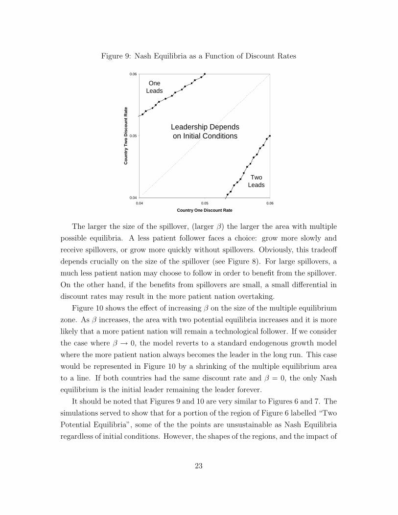
Figure 9: Nash Equilibria as a Function of Discount Rates
0.04
0.05
0.06
0.04 0.05 0.06
Country One Discount Rate
Co
un
try
Tw
o D
isco
un
t R
ate
Leadership Depends on Initial Conditions
OneLeads
TwoLeads
The larger the size of the spillover, (larger β) the larger the area with multiple
possible equilibria. A less patient follower faces a choice: grow more slowly and
receive spillovers, or grow more quickly without spillovers. Obviously, this tradeoff
depends crucially on the size of the spillover (see Figure 8). For large spillovers, a
much less patient nation may choose to follow in order to benefit from the spillover.
On the other hand, if the benefits from spillovers are small, a small differential in
discount rates may result in the more patient nation overtaking.
Figure 10 shows the effect of increasing β on the size of the multiple equilibrium
zone. As β increases, the area with two potential equilibria increases and it is more
likely that a more patient nation will remain a technological follower. If we consider
the case where β → 0, the model reverts to a standard endogenous growth model
where the more patient nation always becomes the leader in the long run. This case
would be represented in Figure 10 by a shrinking of the multiple equilibrium area
to a line. If both countries had the same discount rate and β = 0, the only Nash
equilibrium is the initial leader remaining the leader forever.
It should be noted that Figures 9 and 10 are very similar to Figures 6 and 7. The
simulations served to show that for a portion of the region of Figure 6 labelled “Two
Potential Equilibria”, some of the the points are unsustainable as Nash Equilibria
regardless of initial conditions. However, the shapes of the regions, and the impact of
23

Figure 10: The Effect of Increasing Beta
0.04
0.05
0.06
0.04 0.05 0.06
B = 0.2 B = 0.05
TwoLeads
OneLeads
Leadership Depends on Initial
Conditions
increasing the spillover parameter remain unchanged after the simulations exercise.
5 Conclusion
Our model shows that it is possible to have a stable equilibrium where a less patient
nation is the technological leader. This appears to be the current situation in the
world. As judged by savings rates, the United States appears to have one of the
highest discount rates among the industrialized nations yet invests a higher per
capita share of GDP on research and development than any other nation. This
situation is more likely to occur in a world with rapid transfers of technology from
the technological leader to followers.
If we assume that the speed of transfers is increasing over time, we should see
that technological leadership is more persistent over time. With a low transfer
coefficient, a relatively small shock to discount rates will be sufficient to induce
a change in technological leadership. With a large transfer coefficient, leadership
changes require a much larger differential in discount rates.
This may be the case. The US has been the world technological leader for at
least eighty years and arguably for well over a century. There appear to be few signs
that US technological leadership is diminishing. This is a relatively long period of
24

time when compared to other technological leaders over the previous three centuries.
25

References
Aghion, P. and P. Howitt, “A Model of Growth Through Creative Destruction,”
Econometrica, March 1992, 60 (2).
and , Endogenous Growth Theory, Cambridge, MA: MIT Press, 1998.
Barro, Robert J. and Xavier Sala-i-Martin, Economic Growth, Cambridge,
MA: MIT Press, 1995.
Basu, Susanto and David Weil, “Appropriate Technology and Growth,” Quar-
terly Journal Of Economics, November 1998, 113 (4), 1025–54.
Brezis, Paul Krugman, and Tsiddon, “Leapfrogging in International Compe-
tition: A Theory of Cycles in National Technological Leadership,” American
Economics Review, December 1993.
Gerschenkron, Alexander, Economic Backwardness in Historical Perspective,
Cambridge, MA: The Belknap Press, 1962.
Grossman, Gene and Elhanan Helpman, Innovation and Growth in the Global
Economy, MIT press, 1991.
and , “Endogenous Innovation in the Theory of Growth,” Journal of
Economic Perspectives, Winter 1994, 8 (1).
Howitt, Peter, “Endogenous growth and cross country income differences,” AER,
September 2000, 90 (4), 829–46.
Lucas, Robert E., “On the Mechanics Of Economic Development,” Journal of
Monetary Economics, 1988, 22, 3–42.
Mankiw, N. Gregory, David Romer, and David Weil, “A Contribution to
the Empirics of Economic Growth,” Quarterly Journal Of Economics, 1992,
107, 407–437.
Nelson, Richard and Edmund Phelps, “Investment in Humans, Technological
Diffusion, and Economic Growth,” American Economics Review, 1966, 56, 69–
75.
26

Pack, Howard and Larre E. Westphal, “Industrial Strategy and Technological
Change: Theory Versus Reality,” JDE, June 1986, 22 (1), 87–128.
Romer, Paul, “Increasing Returns and Long-Run Growth,” Journal of Political
Economy, 1986, 94, 1002–1038.
, “The Origins of Endogenous Growth,” Journal of Economic Perspectives,
Winter 1994, 8 (1).
27


![Energy taxes and endogenous technological change (Running ...public.econ.duke.edu/~peretto/EnergyTaxes.pdf · [10]); Barsky and Killian, in contrast, argue that they matter very little](https://img.dokumen.tips/doc/110x75/5e95217cddc9b5741668cd9f/energy-taxes-and-endogenous-technological-change-running-perettoenergytaxespdf.jpg)