Embed Size (px)
Citation preview

A111D5 ^73Sb7PUBLICATIONS
Techniques for TreatingUncertainty and Risk in
the Economic Evaluationof Building Investments
Harold E. Marshall
1
1
1 j
S. DEPARTMENT OF COMMERCEitional Institute of Standards and Technology
ST Special Publication 757


NIST Special Publication 757
Techniques for Treating
Uncertainty and Risk in
the Economic Evaluation
of Building Investments
Harold E. Marshall
Applied Economics Group
Mathematical Analysis Division
Center for Computing and Applied Mathematics
National Engineering Laboratory
National Institute of Standards and Technology
Gaithersburg, MD 20899
/ v Xo ,
—
^1—, V
c
X
NOTE: As of 23 August 1988, the National Bureau of
Standards (NBS) became the National Institute of
Standards and Technology (NIST) when President
Reagan signed into law the Omnibus Trade and
Competitiveness Act.
September 1988
U.S. Department of CommerceC. William Verity, Secretary
National Institute of Standards and Technology
Ernest Ambler, Director

Library of Congress
Catalog Card Number: 88-600584
National Institute of Standards
and Technology
Special Publication 757
97 pages (Sept. 1 988)
CODEN: XNBSAV
U.S. Government Printing Office
Washington: 1988
For sale by the Superintendent
of Documents,
U.S. Government Printing Office,
Washington, DC 20402"

PREFACE
This is the fifth in a series of National Institute of Standards and Technology (NIST), formerly the National
Bureau of Standards (NBS), reports on recommended practices for applying economic evaluation methods to
building decisions. 1 The previous four dealt with the theory and application of six economic methods of
analysis: life-cycle costing, net benefits, benefit-to-cost and savings-to-investment ratios, internal rate of
return, and payback. These reports were used as the bases for recommended standard practices published
by the American Society for Testing and Materials (ASTM). Economic measures described from applying
these methods in project evaluations were presented in the NBS reports and ASTM standards primarily in
single-value, deterministic terms as if all input values were certain.
This report differs from the earlier ones in that it focuses on techniques that account for uncertainty in
input values and techniques that measure the risk that a project will have a less favorable economicoutcome than what is desired or expected. In addition, the report considers techniques for incorporating
risk attitudes of decision makers in selecting efficient projects.
iThe previous four reports are as follows: Rosalie T. Ruegg, Stephen R. Petersen, and Harold E.
Marshall, Recommended Practice for Measuring Life-Cycle Costs of Buildings and Building Systems , National
Bureau of Standards Interagency Report 80-2040, June 1980; Harold E. Marshall and Rosalie T. Ruegg,
Recommended Practice for Measuring Benefit/Cost and Savings-to-Investment Ratios for Buildings and
Building Systems. National Bureau of Standards Interagency Report 81-2397, November 1981; Harold E.
Marshall, Recommended Practice for Measuring Net Benefits and Internal Rates of Return for Investments in
Buildings and Building Systems. National Bureau of Standards Interagency Report 83-2657, October 1983; and
Harold E. Marshall, Recommended Practice for Measuring Simple and Discounted Payback for Investments in
Buildings and Building Systems. National Bureau of Standards Interagency Report 84-2850, March 1984.


ACKNOWLEDGMENTS
Thanks are due the members of ASTM who have participated in the Building Economics Subcommittee
meetings and thereby have helped determine the framework of this paper. Special appreciation is extended
to Tung Au, Robert E. Chapman, Sieglinde K. Fuller, Barbara C. Lippiatt, Margaret S. Murray, Stephen R.
Petersen, Rosalie T. Ruegg, Barry Stedman, James B. Weaver, and Stephen F. Weber for their helpful
technical comments on the paper; to David Rosoff for supplying data for one of the case examples; to
Robert E. Chapman for writing and executing computer programs that produced the simulations and some of
the graphs; and to Laurene Linsenmayer for typing the final manuscript.


GLOSSARY
Adjusted Internal Rate-of-Return (AIRR)-The compound rate of interest that discounts the terminal values
of costs and benefits of a project over a given study period so that costs equal benefits, where terminal
values are computed at a specified reinvestment rate. The AIRR method is used to measure project worth.
Annual Value (Annual Worth)—Project costs or benefits expressed as uniform annual amounts, taking into
account the time value of money.
Base Time (Base Year)-The date (usually the beginning of the study period) to which benefits and costs
are converted to time equivalent values when using the present value method.
Benefit-to-Cost Ratio-The ratio of benefits to costs, where both are discounted to present or annual
values. The BCR method is used to measure project worth.
Breakeven Analysis—A technique for determining the minimum or maximum value that a variable can reach
and still have a breakeven project; i.e., a project where benefits (savings) equal costs.
Capital Asset Pricing Model (CAPM)-The capital asset pricing model explains how assets should be priced
according to their calculated risk and expected returns. It indicates what the return on an asset should be,
based on that asset's risk.
Cash Flow-The stream of costs and benefits resulting from a project investment.
Certain Equivalent FaCtor(CEF)-The factor by which uncertain project returns are multiplied to determine
the "certainty equivalent" amount a decision maker finds equally acceptable.
Certainty Equivalent Technique-A technique used to adjust economic measures of project worth to reflect
risk exposure and risk attitude. Estimated project returns are multiplied by a certainty equivalent factor
(CEF) to determine the "certainty equivalent" amount a decision maker finds equally acceptable.
Coefficient of Variation (CV)-The ratio of the standard deviation to the mean.
Constant Dollars (Real Dollars)-Dollars of uniform purchasing power tied to a specified time.
Contour Lines-Line segments that connect the various rays of a spider diagram.
Cost Effective-The condition whereby the present value benefits (savings) of an investment alternative
exceeds its present value costs.
Cumulative Distribution Function (cdf)-A function that shows on the y axis the probability of a value being
less than or equal to the corresponding value on the x axis.
Current Dollars-Dollars of nonuniform purchasing power, in which actual prices in the market are stated
for any given time. With no inflation or deflation, current dollars will be identical to constant dollars.
Decision Ana lysis-A technique for making economic decisions in an uncertain environment that allows a
decision maker to include alternative outcomes, risk attitudes, and subjective impressions about uncertain
events in an evaluation of investments. Decision analysis typically uses decision trees to represent
decision problems.
vii

Decision Tree-A decision flow diagram (in the shape of a tree) that is used to represent all possible
outcomes, costs, and probabilities associated with a given decision problem. The tree serves as a road mapto clarify possible alternatives and outcomes of sequential decisions.
Differential Price Escalation Rate--The expected percent difference between the rate of increase assumed
for a given item of cost (such as energy), and the general rate of inflation.
Discount Factor--A multiplicative number that is used to convert costs and benefits occurring at different
times to a common time. Discount factors are calculated from a discount formula for a given discount rate
and study period.
Discount Rate-The minimum acceptable rate of return used in discounting benefits and costs occurring at
different times to a common time. Discount rates reflect the investor's time value of money (or
opportunity cost). Real discount rates reflect time value apart from changes in the purchasing power of
the dollar (i.e., inflation or deflation) and are used to discount constant dollar cash flows. Nominal
discount rates include changes in the purchasing power of the dollar and are used to discount current dollar
cash flows.
Discounting-A procedure for converting a cash flow that occurs over time to an equivalent amount at a
common time.
Economic Evaluation Methods-Various ways in which project benefits and costs can be combined and
presented to describe measures of project worth. Examples are life-cycle costs (LCC); net benefits (NB) or
net savings (NS); benefit-to-cost ratio (BCR) or savings-to-investment ratio (SIR); and adjusted internal
rate of return (AIRR).
Future Value (Future Worth)-The value of a cost or benefit at some time in the future, taking into
consideration the time value of money.
Inflation-A rise in the general price level. Inflation can also be described as a decline in the general
purchasing power of a currency.
Internal Rate of Return-The compound rate of interest that, when used to discount a project's cash flows,
will equate costs and benefits.
Investment Costs-The costs associated with acquiring an asset, including such items as design, engineering,
purchase, and installation.
Life-Cycle Cost (LCC)-The sum of all discounted costs of acquiring, owning, operating and maintaining a
building project over the study period. Comparing life-cycle costs among mutually exclusive projects of
equal performance is one way of determining relative cost effectiveness.
Mathematical/Analytical (M/A) Technique-A technique of obtaining probability functions for economic
measures of project worth without the repeated trials of simulation.
Mean (/i)--A statistical measure of central tendency. Specifically, the arithmetic mean is the sum of
individual values for a group of items divided by the number of items in the group. It may also be
referred to as the "average" or "typical" value in a distribution.
Mean-Variance Criterion—A technique for evaluating the relative risk and return when choosing among
competing projects. The mean-variance criterion dictates that the project with the higher mean (i.e.,
expected value of project worth) and lower standard deviation be chosen. This presumes that decision
makers prefer less risk to more risk.
viii

Minimum Acceptable Rate of Return--The minimum percentage return required for an investment to beeconomically acceptable.
Modified Uniform Present Value Factor (UPV*)--The discount factor used to convert an annual amountescalating at a constant rate to a time-equivalent present value.
Mutually Exclusive--A condition where the acceptance of one alternative precludes acceptance of others.
Net Benefits (Savings)-The difference between benefits (savings) and costs, where both are discounted to
present or annual values. The NB method is used to measure project worth.
Nominal Discount Rate -See Discount Rate.
Non-Mutually Exclusive Project-A project whose acceptance does not preclude acceptance of others.
Payback Period-The time it takes for an investment's cumulative benefits or savings from a project to pay
back the investment and other accrued costs.
Portfolio Analysis-A technique used to seek the combination of assets with the maximum return for any
given degree of risk (i.e., variance of the return), or the minimum risk for any given rate of return.
Present Value (Present Worth)-The time-equivalent value at the base time of past, present, or future cash
flows.
Probability Density Function (pdf)-The derivative of a continuous, cumulative distribution function. Thearea under the pdf must equal 1.
Real Discount Rate -See Discount Rate.
Real Dollars -See Constant Dollars.
Resale Value (Salvage Value)-The monetary amount expected from the sale of an asset at its time of
disposal, less disposal costs.
Retrofit—The modification of an existing building or facility to include new systems or components.
Risk-Adjusted Discount Rate (RADR)-A discount rate that has been adjusted to account for risk. Whenusing the RADR technique, projects with anticipated high variability in distributions of project worth have
their net benefits or returns discounted at higher rates than projects with low variability.
Risk Analysis-The body of theory and practice that has evolved to help decision makers assess their risk
exposures and risk attitudes so that the investment that is "best for them" can be selected. (Note that this
definition is restricted to the types of analyses described in this report, and is not necessarily consistent
with how the term is used in reference to analyses in such areas as the environment or health.)
Risk Attitude-The willingness of decision makers to take chances or gamble on investments of uncertain
outcome. Risk attitudes are generally classified as risk averse, risk neutral, or risk taking. Risk averse
decision makers would prefer a sure cash payment to a risky venture with known expected value greater
than the sure cash payment. Risk neutral decision makers act on the basis of expected monetary value.
They would be indifferent between a sure cash payment and a risky venture with expected value equal to
the sure cash payment, and would therefore accept a fair gamble. Risk takers prefer a risky venture with
known expected value to a sure cash payment equal to the expected value.
Risk Averse (RA)-See Risk Attitude.
ix

Risk Exposure—The probability of investing in a project whose economic outcome is different from what is
desired (the target) or what is expected.
Risk Neutral (RN)--See Risk Attitude.
Risk Taking (RT)-See Risk Attitude.
Salvage Value- See Resale Value.
Savings-to-lnvestment Ratio (SIR)-The ratio of present value savings to present value investment costs.
Also computed as the ratio of annual value savings to annual value investment costs. The SIR method is
used to measure project worth.
Sensitivity Analysis—A technique for measuring the impact on project outcomes of changing one or more
key input values about which there is uncertainty.
Single Present Value Factor (SPV)-The discount factor used to convert future benefit and cost values to
time-equivalent present values
Simulation—A technique that can be used to determine risk exposure from an investment decision. Toperform this type of simulation, probability functions of the input variables are required.
Spider Diagram-A graph that presents a snapshot of the potential impact, taking one input at a time, of
several uncertain input variables on project outcomes.
Standard Deviation (a)--The square root of the variance. The standard deviation indicates the extent to
which items in a distribution differ from the mean value.
Study Period (Time Horizon)-The length of time over which an investment is evaluated.
Time Horizon-See Study Period.
Time Value of Money-The time-dependent value of money arising both from the real earning potential of
an investment over time and from changes in the purchasing power of money (i.e., inflation or deflation).
Uncertainty-Uncertainty (or certainty) as used in this report refers to a state of knowledge about the
variable inputs to an economic analysis. If the analyst is unsure of input values, there is uncertainty. If
the analyst is sure, there is certainty.
Uniform Present Value Factor (UPV)-The discount factor used to convert uniform annual values to a time-
equivalent present value.
Utility Function—A function that shows how utility (i.e., satisfaction) varies with money or income. The
utility function shows the decision maker's risk attitude.
Variance (ct2)-A statistical measure of dispersion about the mean. The square root of the variance is the
standard deviation.
x

ABBREVIATIONS AND SYMBOLS
AIRR adjusted internal rate of return
BCR benefit-to-cost ratio
CAPM capital asset pricing model
cdf cumulative distribution function
CEF certainty equivalent factor
CV coefficient of variation
EMV expected monetary value
EMV'er decision maker who acts on the basis of
expected monetary value
HVAC heating, ventilating, and air conditioning
kWh kilowatt hour
LCC life-cycle cost
MARR minimum acceptable rate of return
NB net benefits
NS net savings
NBS National Bureau of Standards
NIST National Institute of Standards and
Technology (formerly NBS)
M/A mathematical /analytical
pdf probability density function
RA risk averse
RADR risk-adjusted discount rate
RN risk neutral
RT risk taking
SIR savings-to-investment ratio
SPV single present value (worth) factor
UPV uniform present value (worth) factor
UPV* modified uniform present value (worth)
factor
|x mean or expected value
cr standard deviation
cr2
variance
xi


CONTENTS
Page
PREFACE iii
ACKNOWLEDGMENTS v
GLOSSARY vii
ABBREVIATIONS AND SYMBOLS xi
1. INTRODUCTION 1
1.1 Background 1
1.2 Purpose 2
1.3 Approaches to Treating Uncertainty and Risk 2
1.4 Organization 3
2. METHODS OF ECONOMIC ANALYSIS AND PROBLEM ILLUSTRATIONS 5
2.1 Methods 5
2.2 Problem Illustration— Uncertainty and Risk Ignored 8
2.2.1 Life-Cycle Cost 9
2.2.2 Net Savings 10
2.2.3 Savings-to-Investment Ratio 11
2.2.4 Adjusted Internal Rate of Return 11
3. RISK EXPOSURE AND RISK ATTITUDE 13
3.1 Risk Exposure 13
3.2 Risk Attitude 15
4. TECHNIQUES THAT DO NOT USE PROBABILITY 23
4.1 Conservative Benefit and Cost Estimating 23
4.2 Breakeven Analysis 23
4.3 Sensitivity Analysis 24
4.3.1 Spider Diagram 26
4.3.2 Contour Lines 27
4.3.3 Spider Diagrams for Competing Projects 29
4.4 Risk-Adjusted Discount Rate 30
4.5 Certainty Equivalent Technique 32
5. TECHNIQUES THAT USE PROBABILITY 35
5.1 Input Estimation Using Expected Values 35
5.2 Mean-Variance Criterion and Coefficient of Variation 36
5.3 Decision Analysis 37
5.3.1 Decision Analysis of Energy Conservation Investment 37
5.3.2 Advantages and Disadvantages of Decision Analysis 41
5.4 Simulation 43
5.4.1 Storage Facility Simulation Example 44
5.4.2 Construction Contingency Simulation Example 52
5.4.3 Advantages and Disadvantages of Simulation 54
5.5 Mathematical /Analytical Technique 55
5.5.1 Shopping Centers Example of M/A Technique 56
5.5.2 Advantages and Disadvantages of M/A Technique 64
5.5.3 M/A Technique Used with the CEF and RADR Techniques 65
5.6 Other Techniques 66
5.6.1 Portfolio Analysis 66
5.6.2 Capital Asset Pricing Model 67
6. CONCLUSIONS 68
xiii

Page
APPENDIX A. Formulas for Calculating Economic Measures 73
APPENDIX B. Constructing a Utility Function 75
BIBLIOGRAPHY 79
SUBJECT INDEX 83
xiv

LIST OF TABLES
Page
Table 1-1. Techniques that account for uncertainty, risk, or both 3
Table 2-1. Methods of economic analysis 6
Table 2-2. Examples of building investment decisions that are evaluated with economic analysis 7
Table 2-3. Data for evaluating new-technology building component
Table 4-1. A firm's certainty equivalent factor table for use in adjusting net cash flows from
uncertain investments 33
Table 5-1. Expected value of reduction in kilowatt hours 35
Table 5-2. Fixed investment and retrofit package cost for buildings I and II 38
Table 5-3. Possible benefit outcomes and their estimated probabilities of occurrence for the six
retrofit packages 39
Table 5-4. Fixed input data for simulation of investment in storage facility 45
Table 5-5. Assumptions for the economic evaluation of the limited-partnership shopping centers 56
Table 5-6. Probability distributions and means, by year, for net cash flows from shopping centers 58
Table 5-7. Standard deviations, by year, for net cash flows from shopping centers 60
Table 5-8. Data for constructing probability density function of present value net cash flows
for shopping centers 61
Table 5-9. Data for constructing cumulative distribution function of present value net cash
flows for shopping centers 63
Table 6-1. Characteristics of techniques for treating uncertainty and risk 69
Table A-l. Formulas useful for measuring the economic worth of building investments 73
Table B-l. Data for plotting utility functions 77
xv

LIST OF FIGURES
Page
Figure 3-1. Probability distribution of benefit-to-cost ratio 14
Figure 3-2. Cumulative distribution function of benefit-to-cost ratio 15
Figure 3-3. Probability density functions of benefit-to-cost ratio for projects A and B 16
Figure 3-4. Cumulative distribution functions of benefit-to-cost ratio for projects A and B 17
Figure 3-5. Intermingled probability density functions of benefit-to-cost ratio for projects Cand D 18
Figure 3-6. Cumulative distribution functions of benefit-to-cost ratio for projects C and D 18
Figure 3-7. Three types of risk attitude 19
Figure 3-8. Utility function showing both risk averse (RA) and risk taking (RT) attitudes 21
Figure 4-1. Sensitivity of net benefits of projects A and B to discount rate 25
Figure 4-2. Spider diagram showing sensitivity of the adjusted internal rate of return to variations
in uncertain variables 27
Figure 4-3. Spider diagram with a contour 28
Figure 4-4. Spider diagrams for competing projects 29
Figure 5-1. Decision tree for conservation investment 40
Figure 5-2. Probability distribution of net benefits for alternative outcomes from R2 42
Figure 5-3. Cumulative distribution function of net benefits for alternative outcomes from R2 43
Figure 5-4. Probability density function of number of units rented 46
Figure 5-5. Probability density function of present value operating costs. 46
Figure 5-6. Probability density function of present value resale price 46
Figure 5-7. Probability density function of present value of land preparation and construction
costs 46
Figure 5-8. Cumulative distribution function of net benefits for the storage facility 49
Figure 5-9. Cumulative distribution function of benefit-to-cost ratio for the storage facility 50
Figure 5-10. Cumulative distribution function of adjusted internal rate of return for the storage
facility 51
Figure 5-11. Two cumulative distribution functions of net benefits for the storage facility 52
Figure 5-12. Contingency /risk graph for construction project X 53
xv i

Page
Figure 5-13. Probability density function of present value net cash flows for shopping centers 62
Figure 5-14. Cumulative distribution function of present value net cash flows for shopping centers. ... 63
Figure B-l. Three types of risk attitude: data and fitted functions 77
xvii


1. INTRODUCTION
1.1 Background
Investments in long-lived projects such as buildings are characterized by uncertainties regarding project
life, operation and maintenance costs, revenues, and other factors that affect project economics. Since
future values of these variable factors are generally not known, it is difficult to make reliable economic
evaluations.
The traditional approach to project investment analysis is to apply economic methods of project evaluation
to "best estimates" of project input variables as if they were certain estimates and then to present results
in single-value, deterministic terms. When projects are evaluated without regard to uncertainty of inputs
to the analysis, decision makers have insufficient information to measure and evaluate the risk of investing
in a project having a different outcome from what is expected.
Although the technical literature treats uncertainty and risk analysis extensively, a recent survey shows
that applications are still far behind theoretical capabilities.3 Several reasons might be hypothesized for
this lag in implementation. First, practicing analysts anticipate high costs and time-consuming analyses in
evaluating risk. Yet computers reduce considerably the costs and time for risk analysis. Second, analysts
are concerned about the lack of data. The more uncertain the input data, however, the more helpful it
would be to account for the uncertainty and to evaluate the associated risk. Third, decision makers,
particularly top managers in corporations or government agencies, are reluctant to accept these techniques
because they are not confident that the techniques will help them make better decisions. This reluctance
may stem in part from a lack of understanding of the techniques. A comprehensive examination of the
different approaches to treating uncertainty and risk in project evaluation would show how the application
of risk analysis techniques to uncertain data can improve management decision making.
This report is intended as the basis for a new ASTM standard on how to account for uncertainty and risk
in economic evaluations of buildings and building components. The approach is tutorial and relatively
comprehensive to build understanding of the appropriate concepts and techniques among engineers,
zSee, for examples, W. Fellner, Probability and Profit (Homewood, Illinois: Richard D. Irwin, Inc.,
1965); Frank H. Knight, Risk, Uncertainty, and Profit (New York, New York: Harper and Row, 1965); D.
Hertz, "Risk Analysis in Capital Investment," Harvard Business Review, January 1964, pp. 95-106; E. C.
Capen, "The Difficulty of Assessing Uncertainty," Journal of Petroleum Technology, August 1976, pp. 843-
850; Michael W. Curran, "Range Estimating for Plaudits and Profits," Baltimore Engineer, April 1986, pp. 6-8;
Raymond P. Lutz and Harold A. Cowles, "Estimation Deviations: Their Effect Upon the Benefit-Cost Ratio,"
The Engineering Economist, Vol. 16, No. 1, pp. 22-42; F. J. Weston and E. F. Brigham, Managerial Finance
(Hinsdale, Illinois: The Dryden Press, 1981); T. Au and T. P. Au, Engineering Economics for Capital
Investment Analysis (Boston, Massachusetts: Allyn and Bacon, Inc., 1983); J. J. Clark, T. J. Hindelang, and
R. E. Pritchard, Capital Budgeting: Planning and Control of Capital Expenditures (Englewood Cliffs, NewJersey: Prentice-Hall, Inc., 1984); Jack Hirshleifer and David L. Shapiro, "The Treatment of Risk and
Uncertainty," ed. Robert Haveman and Julius Margolis, 2nd ed., Public Expenditure and Policy Analysis, 1977,
pp. 180-203; J. E. Matheson and R. A. Howard, "An Introduction to Decision Analysis," Readings in Decision
Analysis (Menlo Park, California: Stanford Research Institute, 1977, pp. 7-43); and Howard Raiffa, Decision
Analysis: Introductory Lectures on Choices Under Uncertainty (Reading, Massachusetts: Addison-Wesley,
1970).
3See, for examples, Suk H. Kim and Edward J. Farragher, "Current Capital Budgeting Practices,"
Management Accounting. June 1981, pp. 26-28; Edward J. Farragher, "Capital Budgeting Practices of Non-
Industrial Firms," The Engineering Economist, Vol. 31, No. 4, Summer 1986, p. 298; and C. Gurnani, "Capital
Budgeting: Theory and Practice," The Engineering Economist, Vol. 30, No. 1, Fall 1984, pp. 32-33.
1

architects, and economists of the American Society for Testing and Materials (ASTM) Subcommittee who will
develop the new standard. The report is also intended for professionals, educators, students, and managers
who are interested in applying these techniques to the economic evaluation of buildings.
1.2 Purpose
The report has two purposes. The first is to describe in depth various techniques for treating uncertainty
and risk in project evaluation. The second is to describe advantages and disadvantages of each technique
to help the decision maker choose an appropriate one for a given problem.
Although the focus is on buildings and building components, the techniques described in this report are
equally applicable to non-building investments. These same principles apply in the evaluation of any capital
budget expenditure whose future stream of benefits, revenues, savings, or costs is uncertain.
1.3 Approaches to Treating Uncertainty and Risk
The numerous treatments of uncertainty and risk that appear in the technical literature come from various
fields including decision analysis, finance, statistics, and economics. For example, the financial literature
defines business risk, investment risk, portfolio risk, cataclysmic risk, financial risk, systematic risk, and
unsystematic risk.
For purposes of this paper, however, uncertainty and risk are defined as follows. Uncertainty (or
certainty) refers to a state of knowledge about the variable inputs to an economic analysis. If the analyst
is unsure of input values, there is uncertainty. If the analyst is sure, there is certainty. Sensitivity
analysis is an example of a technique that accounts for uncertainty. It provides a range of measures of
project worth that corresponds to a range of possible input values.
Risk refers either to risk exposure or risk attitude. Risk exposure is the probability of investing in a
project that will have a less favorable economic outcome than what is desired (the target) or from what is
expected.^ Probability distributions of measures of project worth describe risk exposure. Simulation is an
example of a technique that can be used to build probability distributions that show risk exposure.
Risk attitude, also called risk preference, is the willingness of a decision maker^ to take a chance or
gamble on an investment of uncertain outcome. The implications of decision makers having different risk
attitudes is that a given investment of known risk might be economically acceptable to an investor who is a
risk taker, but totally unacceptable to another investor who is risk averse. Decision analysis is an example
of a technique that uses utility functions to account for risk attitude.
Table 1-1 presents 10 techniques for treating uncertainly and risk described in this report. All of the
techniques account in some way for uncertainty in input values, but not all treat risk. Furthermore, not all
of the techniques in table 1-1 that account for risk treat both risk exposure and risk attitude.
Also included in the report, but not shown in table 1-1, are some techniques for evaluating risk and return
used in managing stock portfolios. These hold some promise as techniques for evaluating portfolios of
building assets.
^he risks listed earlier from the financial literature are in the risk-exposure category. Manyapplications of risk analysis treat exposure risk exclusively.
^A decision maker or investor can be an individual (e.g., chief executive officer) or a group (e.g.,
board of directors).
2

No single technique in table 1-1 can be labeled the "best" technique in every situation for treating
uncertainty, risk, or both. What is best depends on the following: availability of data, availability of
resources (time, money, expertise), computational aids (e.g., computer services), user understanding, ability
to measure risk exposure and risk attitude, risk attitude of decision makers, level of risk exposure of the
project, and size of the investment relative to the institution's portfolio.
Table 1-1. Techniques that account for uncertainty, risk, or both
1. Conservative Benefit and Cost 6. Input Estimation Using ExpectedEstimating Values
2. Breakeven Analysis 7. Mean-Variance Criterion andCoefficient of Variation
3 . Sensitivity Analysis8. Decision Analysis
4. Risk-Adjusted Discount Rate9. Simulation
5. Certainty Equivalent Technique10. Mathematical/Analytical Technique
1.4 Organization
Chapter 2 introduces four common economic methods for evaluating building investments: life-cycle costing;
net benefits or net savings; benefit-to-cost ratio or savings-to-investment ratio; and adjusted internal rate
of return. Appropriate applications for each are specified. Widespread use of the methods in building
evaluations is documented.
An investment problem is analyzed using each of the four methods in the simple, deterministic approach to
capital investment analysis in which uncertainty and risk are ignored in the formal analysis. These problem
examples are presented for two reasons. First, they introduce the methods to readers who are not familiar
with them. This is important because these are the methods with which the techniques for treating
uncertainty and risk are later Illustrated. Second, the examples of the methods with no treatment of
uncertainty and risk provide a baseline against which advantages and disadvantages of the 10 techniques
listed in table 1-1 can be compared. (Readers familiar with the four economic methods and then-
appropriate applications may prefer to pass over chapter 2.)
Chapter 3 provides statistical and economic bases for interpreting the techniques for treating uncertainty
and risk. First, it explains the concept of risk exposure and how it can often be quantified with
cumulative distribution functions and statistical measures of dispersion. Then it introduces the concept of
risk attitude and describes how utility functions can be used to assign values to project outcomes that
reflect decision makers' attitudes toward risk taking.
The 10 techniques for treating uncertainty and risk are presented in chapters 4 and 5. Chapter 4 focuses
on techniques that treat uncertainty and/or risk with single- or multiple-value data. Chapter 5 focuses on
techniques that employ probability distributions of data. In each chapter the techniques are presented
generally in order of increasing complexity. Advantages and disadvantages are described for each technique.
3

Chapters 4 and 5 also provide case examples of building investment problems that illustrate specific
techniques for treating uncertainty and risk. Since relatively brief treatments are given to the theory
underlying each technique, case examples are relied upon in part to explain the techniques. Actual project
data and typical building problems are used to some extent to provide "real-world" illustrations of building
investment decisions. Note, however, that the economic results for any case example relate only to defined
conditions and cannot be generalized for that type of investment.
Chapter 6 concludes the report with a table of comparative characteristics for all of the techniques and
guidance on how to choose among the techniques. Appendix A provides a table of formulas for the four
economic methods (life-cycle costing, net benefits, benefit-to-cost ratio, and adjusted internal rate of
return) with which risk analysis might properly be applied. And appendix B explains and illustrates the
process of deriving a utility function for measuring risk attitude.
4

2. METHODS OF ECONOMIC ANALYSIS AND PROBLEM ILLUSTRATIONS
This chapter describes four standard methods of economic analysis and their use in the private and public
sectors. It also provides numerical illustrations of each method applied to a building investment problem.
The techniques for treating uncertainty and risk described in chapters 4 and 5 are used in conjunction with
these economic methods. Thus an understanding of the methods is necessary to use the techniques
described in chapters 4 and 5. The numerical illustrations also make clear the deterministic nature of
typical applications of the methods.
2.1 Methods
Table 2-1 lists four common methods^ used in evaluating capital investment projects, the unit measure of
project worth used for each of the methods, and the appropriate applications for each7 These traditional
methods are used in evaluating four basic types of building decisions: accepting or rejecting a given
building investment, choosing the cost-effective design of a building or component, choosing the cost-
effective size of a building or component, and choosing the economically efficient combination of projects
competing for a limited budget. Examples of some of these types of decisions for the building industry are
given in table 2-2.
Both industry and government use the methods in table 2-1 for making building (as well as non-building)
investment decisions. For example, the American Society for Testing and Materials (ASTM), with over
30,000 members representing industry, government, and academia, has published through its building
economics subcommittee standard practices for each of the methods in table 2-1.^ Professional societies,
such as the American Institute for Architects (AJA)9 and the American Society of Heating, Refrigerating,
and Air Conditioning Engineers (ASHRAE)-^ also have published guidelines for making economic evaluations
of buildings and building components using methods listed in table 2-1.
Federal, state, and local government agencies use the economic methods in the analysis of building design
and operation. The Department of Energy was directed by Executive Order and legislation to provide
"practical and effective" methods and procedures to Federal agencies for estimating life-cycle costs and
savings of proposed energy conservation and renewable energy projects and for comparing their cost
effectiveness in a uniform and consistent manner among agencies. These methods and procedures were
developed for the Department of Energy at the National Institute of Standards and Technology.12 They are
now being applied to more than 400,000 Federal buildings.
^Those readers who are familiar with the methods described in table 2-1 may prefer to go directly to
chapter 3.
'Payback period is left out because it is not an appropriate technique for making many kinds of
investment decisions.
^American Society for Testing and Materials, Annual Book of Standards, Vol. 04.07 (Philadelphia,
Pennsylvania: ASTM, 1987).
9See Harold E. Marshall and Rosalie T. Ruegg, Simplified Energy Design Economics: Principles of
Economics Applied to Energy Conservation and Solar Energy Investments in Buildings , National Bureau of
Standards Special Publication 544, Reprinted by American Institute of Architects, January 1980.
^American Society of Heating, Refrigerating and Air-Conditioning Engineers, Inc., "Life-Cycle
Costing," ASHRAE Handbook , Chapter 42 (Atlanta, Georgia: ASHRAE, 1984).
1:LU.S. Congress, National Energy Conservation Policy Act, November 1978, Title V, Part 3, Sec. 545(a).
12See Rosalie T. Ruegg, Life-Cycle Costing Manual for the Federal Energy Management Program,
National Bureau of Standards Handbook 135 (Rev. 1987), November 1987, and Rosalie T. Ruegg and Stephen
R. Petersen, Comprehensive Guide for Least-Cost Energy Decisions , National Bureau of Standards Special
Publication 709, January 1987 for these methods and procedures.
5

Table 2-1. Methods of economic analysis'1
Unit MeasureName of Worth Applications
(1) Life-Cycle Cost (LCC) $
and
(2) Net Savings (NS) $
or
Net Benefits (NB) $
* Determine if a project should beaccepted
,
* Choose the size or scale of a
project, and
* Choose among alternative projectdesigns competing for a givenpurpose
.
(3) Benefit-to-Cost (BCR) Ratio
or
RatioSavings - to - Investment(SIR)
and%
(4) Adjusted Internal Rateof Return (AIRR) C
* Determine if a project should beaccepted
,
* Choose the size or scale of a
proj ectb, and
* Establish priority and chooseamong non-mutually exclusiveprojects competing for a limitedbudget
.
a See appendix A for formulas for these methods.
b For this application, marginal BCRs (SIRs) or AIRRs are required.
c The internal rate of return adjusted for reinvestments of investment earnings at
explicit rates is used throughout this report. This differs from the traditionalinternal rate of return which makes the unlikely assumption that reinvestmentsachieve the same rate earned on the original investment. For a comparison of
the adjusted and traditional internal rates of return, see Marshall, Harold E.,
"Advantages of the Adjusted Rate of Return," Cost Engineering , Vol. 28, No. 2,
February 1986, pp. 32-37.
6

Table 2-2. Examples of building investment decisions that are evaluated with economicanalysis
Type of Decision Example
Acceptance/Rejection * Will the purchase of a particular rental warehouse beprofitable?
* Is a time clock system for managing HVAC equipment costeffective?
* Is a solar hot water system cost effective?
* Is a fire sprinkler system cost effective?
* Will insulation be cost effective for a water heater?
Design * Which heating system among several alternatives is mostcost effective?
* Which plumbing system is most cost effective?
* What kind of insulation (e.g., foam, fiberglass,cellulose) is most cost effective?
* Is single, double, or triple glazing most costeffective?
* Which floor finish (e.g., carpeting, tile, wood) is mostcost effective?
* Which wall type (e.g., masonry, wood frame, curtainwall) is most economical?
Size * What is the economically efficient level (R-value) ofinsulation in the walls and above the ceiling of a
house?
* How many square feet of collector area and what storagevolume should be provided for a solar energy system?
Priority * What combination of investments in a given building(e.g., new water heater, new floor tile, and newlighting system) is economically preferred when each is
justifiable on economic grounds, but insufficient funds
are available to pay for all of them?
7

The General Services Administration, responsible for providing all Federal space, uses the life-cycle cost
(LCC) economic method in routine investments as well as in determining whether to build or lease newspace. State and local government agencies are also implementing economic evaluation methods both for
facilities and procurement. Twenty-six states were using economic evaluation methods by 1981.^
Risk exposure and risk attitude are seldom treated in these public evaluations. The ASTM recommendedpractices, the Department of Energy guidelines, and the state and local government procedures, however, do
treat uncertainty in that they recommend sensitivity analysis.
The absence of risk analysis in practice does not suggest any shortcoming in the economic methods
described in table 2-1. The methods are generally well known and accepted. The possible weakness in
capital investment analysis in practice is in failing to account adequately for uncertainty and risk whenusing the methods, thereby giving decision makers an incomplete economic picture. The following problem
illustrates typical applications of economic methods without consideration of uncertainty and risk.
2.2 Problem Illustration— Uncertainty and Risk Ignored
An economic analysis is presented for determining if a new-technology building component should be
accepted. The component could be a new kind of roofing system, a new type of heating/cooling element, or
any other item that is being considered either for a new building or for a building retrofit. The new-
technology component is evaluated with each of the four economic methods listed in table 2-1: life-cycle
cost (LCC), net savings (NS), savings-to-investment ratio (SIR), and adjusted internal rate of return (AIRR).
The formulas for computing the economic measures are based on those in appendix A. With the exception
of eq (2.4) for the AIRR, however, all equations in chapter 2 are expressed in a slightly different form
from appendix A to allow the use of discount factors in calculating present values of specific costs and
benefits.
Table 2-3 lists the assumptions for the building problem to which the four economic methods will be
applied. The new-technology component costs $6,000 more than the existing-technology alternative, but
saves $500 annually in maintenance. The new-technology component is expected to last at least 20 years,
the study period for the analysis, while the existing-technology component is expected to last only 10 years.
Thus no replacements are required for the new-technology component, but one replacement at the end of
10 years can be expected for the existing-technology component. No salvage value is expected for either
component. All costs are expressed in constant dollars. The real discount rate and minimum acceptable
rate of return (MARR) are 10 percent. The analysis is for a public building, so taxes need not be
considered.
It is assumed that the components perform equally well. Thus the problem is to determine if it is cost
effective to invest an additional $6,000 for a new-technology component in order to avoid extra replacement
and annual maintenance costs required by installing the existing-technology component. Table 2-1 indicates
this acceptance/rejection problem to be an appropriate application for any of the four methods.
-^Alphonse Dell'Isolla and Stephen J. Kirk, Life-Cycle Costing for Design Professionals (New York,
New York: McGraw-Hill, 1981), p. 174.
l^axes should be included in an economic analysis if the building is owned by a tax-paying institution
because taxes typically play a significant role in the building's economic performance. Taxes are not
included for most of the examples here in order to simplify and focus on exposition of the methods and
techniques. In section 5.4.1 on simulation, however, a comprehensive analysis including tax effects is
presented to illustrate how an after-tax treatment is done.
8

Table 2-3. Data for evaluating new -technology building component 11
Installation Cost (C)
New- technology Component (CN )
Existing- technology Component (CE )
Annual Maintenance Cost (A)
New- technology Component (MN )
Existing- technology Component (ME )
Study Period (N)
Expected LifeNew- technology ComponentExisting- technology Component
Replacement CostsNew- technology Component (RN )
Existing- technology Component (RE )
Salvage ValueNew- technology Component (S N )
Existing- technology Component (SE )
Discount Rate (i)
Minimum Acceptable Rate of Return (MARR)
$15,000$9,000
$500
$1 ,000
20 years
20 years +
10 years
none
$9 ,000
nonenone
10 percent 13
10 percentb
a All costs are in constant dollars as of the base year.
b The discount rate and MARR are in real terms, meaning that they reflect that
portion of the time value of money related to the real earning power of money
over time. A real discount rate and MARR are required when evaluating future
costs and benefits that are denominated in constant dollars.
2.2.1 Life-Cycle Cost
The LCC is calculated for the existing-technology and new-technology components using eq (2.1), where all
amounts have been converted to present values. The cost-effective component will be the one with the
lower LCC.
LCC = C + R + A, (2.1)
where LCC = present value of life cycle costs,
C = present value of installation costs,
R = present value of replacement costs, and
A = present value of maintenance, repair, and other annual costs.
9

Since C occurs at the base time, it is already in present value terms. Since R occurs in the future, it has
to be discounted to present value. Maintenance, repair, and other costs occurring on an annual basis must
be converted to present values. The following calculations take the time value of money into consideration
in arriving at the LCC of the existing-technology component (LCCE) and of the new-technology component(LCCN ).
LCCE = CE + RE + AE
= $9,000 + (SPVN = 1o!i== i0%)($9,000) + (UPVN = 20)i = 10%)($l,000)
= $9,000 + (0.3855) ($9,000) + (8.514) ($1,000)
= $9,000 + $3,470 + $8,514
LCCE = $20,984
The LCC of using the existing-technology component is estimated to be $20,984. Note that the word
"estimate" is used. This is because typically the values of replacement, repair, maintenance, and component
life are uncertain, and therefore the LCC estimate will be uncertain.
The LCC for the new-technology component is computed the same way.
LCCjsj = Cjvj + Rjvj + Ajsj
= $15,000 + 0 + (UPVN = 2o,i = iO%)($500)
= $15,000 + 0 + (8.514) ($500)
= $15,000 + 0 + $4,257
= $19,257
Since the LCC of the new-technology component is estimated to be less than that of the existing-
technology component, it appears cost effective to purchase the new-technology component.
2.2.2 Net Savings
Net savings (NS) can also be used to determine if the new-technology component is cost effective.^ Given
that LCCs have already been calculated for the two components, the NS from using the new-technology
component can be determined by subtracting the LCC with the new-technology component (LCCjvj) from the
LCC with the existing-technology component (LCCE), as shown in eq (2.2).
NS = LCCE - LCCN (2.2)
NS = $20,984 - $19,257
NS = $1,727
Since the NS for using the new-technology component instead of the existing-technology one is a positive
amount, the analysis indicates the new technology to be a cost-effective investment.
±JNote that net savings could just as easily be called net benefits. It is referred to here as net
savings only because the benefits from investing in the new-technology component are in the form of
maintenance and replacement savings.
L0

2.23 Savings-to-Investment Ratio
The savings-to-investment ratio indicates a project is cost effective if the ratio is greater than 1.0.
Equation (2.3) can be used to calculate the SIR.
SIR = (AM + AR)/AC, (2.3)
where AM = Mg— Mjsj,
AR = RE—
R
N , and
AC = cN-cE .
If the new-technology component is cost effective, the savings it generates through reductions in
maintenance and replacement costs must exceed the associated increase in initial costs (all in present value
terms). The following calculation shows that the decline in M and R exceed by a factor of 1.29 the $6,000
extra cost of the new-technology component.
SIR = (($8,514-$4,257) + ($3,470- $0))/($15,000- $9,000)
= ($4,257 + $3,470))/$6,000
= $7,727/$6,000
= 1.29
Thus the new component is cost effective based on the SIR estimate.
2.2.4 Adjusted Internal Rate of Return
The last method illustrated is the adjusted internal rate of return (AIRR). The AIRR earned on the new-
technology component must be greater than the minimum acceptable rate of return (MARR) for the
investment to be cost effective. Equation (2.4) can be used to calculate the AIRR.
AIRR =-1.0 + (1 + r)(BCR) 1/N, (2.4)
where r = the rate of return on reinvestments of cash savings, which is
equal to 10 percent (the discount rate) for this problem.
The following calculation produces an AIRR of 11.4 percent. This exceeds the MARR of 10 percent and
therefore suggests that the new component is cost effective.
AIRR =-1.0 + (1 + 0.1)(1.29)1/20
= -1.0 + 1.1 (1.0128)
= 0.114
All four of the economic measures suggest that the project is cost effective. This is not surprising, since
all four should give consistent results when properly applied. Note, however, that all of the measures are
1.1

based on the following uncertain variables: (1) the year in which the existing-technology system is to be
replaced, (2) the year in which the new-technology system is to be replaced, (3) the dollar cost of the
capital replacement of the existing-technology component, (4) annual maintenance and repair costs of the
existing-technology component, and (5) annual maintenance and repair costs of the new-technology
component.
Variations in any of these variables from their assigned values could make the new-technology component
uneconomic. For example, if the old-technology component did not have to be replaced, or the dollar costs
of replacement for it were less than $9,000, or the difference in annual maintenance costs were less than
$500, or any combination of the above, then investing in the new-technology component would be less
desirable and in fact might not be cost effective. Thus it becomes apparent that using "best guess"
estimates in a deterministic approach to evaluating capital investments may lead to uneconomic investment
choices.
This does not mean, however, that single-value, deterministic measures of project worth are not useful. If
input data and measures of worth are not expected to vary much, applying the methods without accounting
for uncertainty and risk may be appropriate.
On the other hand, where wide variations in project worth are possible, and where decision makers have a
strongly positive or negative attitude towards risk taking, techniques are needed to extend the methods to
account for variability in measures of project worth. Chapter 3 defines risk exposure and risk attitude,
shows how they can be measured, and thereby provides the basis for understanding the techniques for
treating uncertainty and risk described in chapters 4 and 5.
L2

3. RISK EXPOSURE AND RISK ATTITUDE
Decision makers faced with investment choices under uncertain conditions are concerned with two aspects
of risk. The first is risk exposure. It is the probability of investing in a project whose economic outcome
is different from what is desired (the target) or what is expected. The second is risk attitude. It is the
willingness of decision makers to take chances or gamble on investments of uncertain outcome. The fact
that decision makers have different risk attitudes means that an investment with a given level of risk
exposure might be economically acceptable to an investor who is a risk taker, but totally unacceptable to
another investor who is more risk averse.
Risk analysis is the body of theory and practice that has evolved to help decision makers assess their risk
exposures and risk attitudes so that the investment that is "best for them" can be selected. This section
distinguishes between risk exposure and risk attitude, discusses how risk exposure can be measured with
probability distributions, and describes how utility functions can be generated and used to account for risk
attitude.
3.1 Risk Exposure
A probability distribution quantifies risk exposure by showing probabilities of achieving different economic
worth values. Figure 3-1 is a discrete probability distribution^ that shows graphically for a building
investment a profile of probabilities for the benefit-to-cost ratio (BCR). Each bar of the histogram shows
on the vertical axis the probability of the investment achieving the corresponding BCR on the horizontal
axis. The mean (expected value) of the BCR is 2.0. This suggests that the most likely measure of worth
will well exceed the 1.0 BCR that is normally regarded as the minimum hurdle necessary for project
acceptance.
Other values for the BCR are possible, however, including a value less than 1.0. Having the standard
deviation and mean for the distribution helps the decision maker determine the likelihood that the actual
BCR is within acceptable bounds around the mean. The smaller the spread of the distribution, as measured
by the standard deviation, the tighter the distribution is around the mean value and the smaller is the risk
exposure associated with the project.
It is known that in a normal distribution the probability is 68.26 percent, 95.46 percent, and 99.73 percent
respectively that the actual value will be within one, two, and three standard deviations of the mean.
Assuming the discrete probability distribution in figure 3-1 approximates a normal distribution, we can
estimate the probability of the BCR being within any one of the standard deviation ranges. The standard
deviation for figure 3-1 is found to be 0.72 by the following eq:
Na = (E(BCRs -^)
2 -Ps)
1/2,
(3.1)
s = l
16Measuring the probability of the project's economic worth being less than the target value reveals
the risk of accepting an uneconomic project. Another type of risk exposure that some decision makers are
concerned about is the probability of passing up a good investment. For example, measuring the
probability of the project's economic worth being greater than the target value reveals the risk of rejecting
an economic project. The risk of accepting an uneconomic project is focused on here.
17The discrete probability distribution is also called probability function and probability mass function.
13

where a = standard deviation
s = possible state,
N = number of possible states
BCRS= BCR in sth state,
(j, = mean or expected value of the distribution, and
Ps= probability of sth state.
Thus we know, for example, there is a 68.26 percent probability that the BCR will lie in the range of 1.28
(2.0 - 0.72) to 2.72 (2.0 + 0.72).
o^ 0.2
0.5 1.0 1.5 2.0 2.5
Benefit-to-Cost Ratio
Figure 3-1. Probability distribution of benefit-to-cost ratio.
Although the probability distribution in figure 3-1 does not reveal directly the probability of choosing a
project having a BCR less than some target value (say, less than the expected value of 2.0 in this case), it
is easily transformed to the cumulative distribution function (cdf) in figure 3-2 which does.1^ Any percent
on the vertical axis in figure 3-2 is read "less than." The function relating BCRs to cumulative
probabilities is upward sloping, indicating that the probability of the BCR being less than any given BCRvalue on the horizontal axis increases as the given BCR value increases.
The probability (or risk of exposure) of the BCR being less than 1.0 is 5 percent in figure 3-2. Or, said
another way, the probability of the project earning positive net benefits or at least breaking even is 95
percent. The probability that the BCR is less than the target value (expected value) of 2.0 is 35 percent.
l^See chapter 5 for a detailed description of how to build a cdf from a probability density function.
L4

0.5 1.0 1.5 2.0 2.5 3.0 3.5 4.0
Benefit-to-Cost Ratio
Figure 3-2. Cumulative distribution function of benefit-to-cost ratio.
Probability and distribution functions provide considerably more information about risk exposure than
deterministic approaches described in chapter 2 that assume certainty and provide single-value measures of
project worth. But the functions in themselves do not treat risk attitude. That is, they show only risk
exposure. Different decision makers, individuals or institutions,^ may respond differently to any given
profile of risk exposure. Thus, to make efficient choices when investment outcomes are uncertain, decision
makers also need to consider their unique risk attitudes.
3.2 Risk Attitude
There are two general approaches decision makers might follow to incorporate risk attitudes in their project
evaluations. First, they can examine the distribution profile, mean, and standard deviation of the measure
of project worth to assess their risk exposure, and then make a decision on the basis of their subjective or
intuitive perception of whether they are prepared to accept the degree of risk exposure indicated. This
informal approach allows for the consideration of risk attitude, but lacks any standard procedure for
measuring personal or institutional risk attitude when making a choice. For example, if the investment
decision is to accept or reject a single project, this approach will often be adequate. Thus the project
described by figure 3-2 is likely to be deemed cost effective by all but the most risk averse decision
makers since there is little probability of a BCR less than 1.0.
19An entity such as a corporation has a risk attitude just like an individual. To determine it,
however, may be difficult. One approach is to use the risk attitude of the chief executive officer as a
proxy for the corporation. Another is to use the attitude of the board of directors.
15

Even where several projects are being compared, the informal approach for considering risk attitude may be
adequate. Although the preferred choice may not be obvious from an examination of probability density
functions (pdfs)^ for individual projects, it may become obvious when functions for alternative projects are
superimposed as shown in figures 3-3 and 3-4. Here the probability profiles are a good index to project
choice because project A clearly has "stochastic dominance" over project B. That is, for every BCR value
in figures 3-3 and 3-4, there is as high or higher probability that project A will exceed that BCR than will
project B. In other words, for every BCR, there is as high or higher probability that project B will provide
a lower or equal BCR than project A. Thus the project alternative whose function is farthest to the right
is the preferred alternative. (Note that if life-cycle costs of alternatives were measured on the horizontal
axis instead of BCRs, the alternative farthest to the left would be preferred because the objective function
would be to minimize life-cycle costs rather than to maximize the BCR.)
Project A
2 3 4
Benefit-to-Cost Ratio
Figure 3-3. Probability density functions of benefit-to-cost ratio for projects A and B.
^UThe probability density function (pdf) is the derivative of a continuous, cumulative distribution
function. The area under the pdf must equal 1.
L6

0 1 2 3 4 5 6
Benefit-to-Cost Ratio
Figure 3-4. Cumulative distribution functions of benefit-to-cost ratio for projects A and B.
The second approach for considering risk attitude is considered formal because it employs a standard
procedure for measuring the decision maker's attitude towards risk and then uses that measure in evaluating
the economic worth of a risky project. The need for a formal technique is illustrated by the intermingled
distributions shown in figures 3-5 and 3-6. Although project D has the larger mean, it also has the larger
variance. That is, the project with the greater expected return also has the greater variance or risk of
exposure. There is no clear indication of stochastic dominance or project preference. Some procedure for
including risk attitude in project evaluation is required to establish project preference in this case.
The remainder of this chapter describes conceptually how risk attitude can be measured and interpreted
through the application of utility theory. Appendix B describes in detail how to construct utility functions.
Risk attitude is measured by the tradeoffs decision makers will make between uncertain money payoffs of
known probability and sure money payoffs. These tradeoffs are determined by asking decision makers to
specify how much sure money (the certainty equivalent) must be received to make them indifferent
between the certainty equivalent and the expected value of a given amount that is not certain. For
example, if a person were given a choice between a lottery, say with a 50 percent probability of winning
$1,000 and a 50 percent probability of winning nothing, and a sure or certain amount of money, there
would be some amount of that certain payment at which the decision maker would be indifferent between
the lottery and the sure payment. The revealed tradeoffs between the expected value of the lottery and
the sure payment determine whether a decision maker is risk neutral, risk averse, or a risk taker. Onceseveral such tradeoffs have been specified, a relationship between money and utility can be determined.^1
Utility here means simply the satisfaction a decision maker receives from given quantities of money.
17

1.00
Figure 3-5. Intermingled probability density functions of benefit-to-cost ratio for projects Cand D.
Benefit-to-Cost Ratio
Figure 3-6. Cumulative distribution functions of benefit-to-cost ratio for projects C and D.
1
8

A graph of this money-utility relationship, called a utility function, can be used to show the decision
maker's risk attitude.22 There are formal techniques for using utility functions in conjunction with the
economic methods described in chapter 2. These techniques help decision makers choose among competing
projects that do not exhibit stochastic dominance like C and D in figures 3-5 and 3-6.
Figure 3-7 shows three shapes of utility functions.23 Each shape represents one of three different risk
attitudes-risk neutral, risk averse, and risk taking. Utility values, displayed on the vertical axis, are
arbitrary units used to measure the degree of utility or satisfaction associated with a given amount of
money shown on the horizontal axis.24 The utility function reflects a particular relationship between
satisfaction, a subjective value, and monetary amounts. Thus the utility function is unique to one
individual, firm, or institution. Each decision maker is likely to have a different utility function.
Figure 3-7. Three types of risk attitude.
RN = risk neutral,
RA = risk averse, and
RT = risk taking
22Because utility theory is used to measure risk attitude, the literature often uses the term "utility
theory" when treating the subject of risk attitude.
23Appendix B describes in detail how the functions in figure 3-7 were derived.
24Note that relative utility-not absolute utility-is being measured. An individual could assign any
two utility values on the vertical axis to any two dollar amounts on the horizontal axis. However, once
those have been assigned, there exists a unique utility value for every other dollar amount.
19

In using the utility function in an economic analysis, it is assumed that a decision maker will be indifferent
among investments with the same expected utility, and prefer investment A to investment B if the expected
utility is greater for A than B.^ The procedure for using the utility function to choose among alternative
investments can be generally described as follows:^ (1) find from the function, for each investment
alternative, utility values that correspond to each dollar-valued outcome in the probability distribution of
potential outcomes; (2) find the expected utility value (the sum of outcome utilities weighted by outcome
probabilities) for each investment; and (3) select the investment with the maximum expected utility.
Given this general background on the construction and use of utility functions, the three utility functions
in figure 3-7 can now be interpreted in some detail. For the straight-line utility function (RN), each
additional, fixed increment of income yields a constant increase in utility; i.e., the marginal utility of
income is constant. The decision maker is considered risk neutral because the gain or loss of a large
amount of money would yield the same increase or decrease respectively in utility per dollar as would the
gain or loss of a small amount of money.
Since the shape of the utility function is dependent on tradeoffs between uncertain money payoffs of known
probability and sure money payoffs, it is also helpful to consider risk attitude directly in terms of how a
decision maker reacts to such gambles. Decision makers who are risk neutral are called EMV'ers because97
they act on the basis of expected monetary value (EMV). For example, the worth or EMV of the lottery
described earlier is calculated as follows:
EMV = 0.5($1,000) + 0.5($0.00) = $500.
An EMV'er would be indifferent to the lottery or a sure cash payment of $500. Hence, the decision maker
is risk neutral in the sense of being willing to accept a "fair" gamble. The utility function for a risk-
neutral decision maker is a straight line, because there is a constant tradeoff between satisfaction in utility
and dollar amounts. An implicit assumption in many economic analyses is that decision makers are EMV'ers.
Thus there is no explicit consideration of risk attitude because maximizing the expected value of net
benefits is assumed to be equivalent to maximizing expected utility.
If the utility function bends over to the right (RA in fig. 3-7), the decision maker is risk averse.
Increasingly large dollar amounts are required to achieve constant increments of utility; i.e., the marginal
utility of income is diminishing. This means that a decision maker would prefer a sure payment that is less
than the expected value of the lottery to the chance of participating in the lottery. In other words, the
amount the decision maker is willing to pay for the lottery ticket will be less than its expected value
because of aversion to the risk of the lottery's outcome. This implies that decision makers regard marginal
payoffs to be worth less (i.e., to be of less utility), per dollar, as total payoffs increase. Thus, to
determine the true value of investments for risk-averse decision makers, economic analyses must account for
decreasing satisfaction of higher payoffs with corresponding decreases in marginal utility. Since empirical
studies have shown that most corporate decision makers are in the risk-averse category,-^ accounting for
risk attitude is a significant consideration in project evaluation.
^The utility theory described in this chapter evolved from that published in The Theory of Games and
Economic Behavior, by John von Neuman and Oskar Morgenstern (Princeton, New Jersey: Princeton
University Press, 1944).
^This procedure is most descriptive of decision analysis, one of the techniques described in chapter 5.
Note that if the measure of worth is not dollars (e.g., a BCR measure) then the projected benefits and
costs are first transformed to utility units before computing the measure of worth.
^Raiffa, Decision Analysis , p. 9.
^See, for examples, Carl S. Spetzler, "Establishing a Corporate Risk Policy," 1986 Proceedings of the
American Institute of Industrial Engineers (Norcross, Georgia: AIIE, 1986), and Ralph O. Swalm, "Utility
Theory-Insights into Risk Taking," Harvard Business Review, Nov./Dec. 1966, pp. 123-136.
20

If the utility function bends upward to the left (RT in fig. 3-7), the decision maker is a risk taker.
Successively smaller dollar amounts are required to achieve constant increments in utility; i.e., the marginal
utility of income is increasing. This implies that the decision maker would actually pay a premium for a
lottery ticket, i.e., a value greater than the expected value of the lottery. The reason is that the decision
maker regards project payoffs to be worth more (i.e., to have more utility), per dollar, as the total payoffs
increase. Thus, to determine the true value of investments for risk takers, economic analyses must account
for increasing marginal satisfaction of higher payoffs with corresponding increases in marginal utility.
Behavior of decision makers implies that more than one risk attitude is possible, depending on the monetary
stakes. For example, many low-income persons are willing to buy insurance at a premium greater than the
expected value of a loss without insurance (sign of risk averter) and at the same time to play the lottery
at worse than fair odds (sign of risk taker). This suggests a utility function with risk averting and risk
taking segments, as shown in figure 3-8.^
Figure 3-8. Utility function showing both risk averse (RA) and risk taking (RT) attitudes.
Note that expected utility analysis based on subjective utility functions will not necessarily predict the way
decision makers will actually choose among alternative investments. Decision makers are not expected to
act rationally and consistently in every investment situation with respect to their revealed utility-money
functions. Friedman and Savage point out that decision makers do not, in fact, calculate utilities before
making every choice.3^ However, utility analysis is still useful as long as decision makers generally act as
29Milton Friedman and L. J. Savage discuss at length various shapes of utility functions in "The Utility
Analysis of Choices Involving Risk," Readings in Price Theory (Homewood, Illinois: Richard D. Irwin, Inc.,
1952), pp. 57-96.
RA RT
5
Income
30Ibid., p. 86.
21

if they had compared expected utilities and as if they knew the odds for the economic choices being
evaluated. Under these conditions, a firm or institution can use utility theory in a normative or
prescriptive role to establish risk policy that will consistently direct management to investments that
support the firm's or institutions's risk attitude.
Several factors have limited the application of risk attitude adjustments in practice. First, many decision
makers consider the technique impractical for their institution. This may be due in part to a lack of
understanding and to an unwillingness to give up some opportunities for personal judgment in project
evaluation. Second, there is often considerable difficulty in determining an organization's risk attitude.
This arises for a couple of reasons. Because individual decision makers may not want to be bound by an
organization's risk policy, they may be unwilling to cooperate in defining that policy. Also, because
individuals are often risk averters in their personal frame of reference, they may have difficulty in
identifying an institutional risk attitude where a more risk-taking attitude might be appropriate.
The use of risk attitude adjustments in project evaluation, however, does have merit. Competent
professional assistance in helping decision makers develop and implement a risk policy would overcome many
of the limiting factors described earlier. There is a sound theoretical basis for including risk attitude
adjustments. And a firm or institution that can establish a risk policy that consistently directs management
to investments that support the firm's or institution's risk attitude will select better projects over the
long run.
In the next two chapters, various techniques of treating risk exposure and risk attitude are described and
illustrated. Some techniques, such as the mathematical/analytical technique, focus on risk exposure, whereas
others, such as the risk-adjusted discount rate, account for risk attitude as well as risk exposure. Aconfusion is often created by the literature because the term "risk analysis" is used sometimes to describe
exclusively either risk exposure or risk attitude, and other times to describe both. Thus in these
illustrations it will be made explicit in each case whether risk exposure, risk attitude, or both are treated.
22

4. TECHNIQUES THAT DO NOT USE PROBABILITY
Chapter 4 describes five techniques that treat uncertainty and risk in project evaluation without using
probability or cumulative distribution functions. Techniques that use such functions are examined in chapter
5. In both chapters, advantages and disadvantages of each technique are described, and the extent to
which each technique accounts for risk exposure and risk attitude is discussed.
4.1 Conservative Benefit and Cost Estimating
A simplistic approach to accounting for the uncertainty of input values is to be conservative in their
estimation so that any error in prediction will likely be an underestimation of project economic worth.
This is accomplished by intentionally estimating benefits on the low side, costs on the high side, or both.
Or, when estimating values of parameters on which benefits and costs depend, such as the discount rate or
project life, the parameter estimates would be made in the direction that lowers expected benefits and
raises expected costs.
The more conservative are benefit and cost estimates, the more assurance one has that a project estimated
to be cost effective will in fact be so. This technique is most useful when a decision maker suffers a great
penalty for selecting an uneconomic project, but incurs no penalty for rejecting economic projects.
However, if a firm were using this technique to determine its bids on construction projects, it would be
unlikely to win many contracts in a competitive market. The technique provides no measure of the risk of
making an uneconomic decision, and it will actually bias decision makers against choosing many projects
that would in fact be economic.
The greater the risk exposure perceived by the decision maker, and the more risk averse the decision
maker, the more conservative will be the benefit and cost estimates. With this technique there is no clear
distinction between adjustments for handling risk exposure and risk attitude.
4.2 Breakeven Analysis
When an uncertain variable is critical to the economic success of a project, decision makers sometimes want
to know the minimum or maximum value that variable can reach and still have a breakeven project; i.e., a
project where benefits (savings) equal costs. For example, the breakeven value of an input cost variable
is the maximum amount one can afford to pay for the input and still break even compared to benefits
earned. A breakeven value of an input benefit variable is the minimum amount the project can produce in
that benefit category and still cover the projected costs of the project.
To perform a breakeven analysis, an equation is constructed wherein the benefits are set equal to the costs
for a given investment project, the values of all inputs except the breakeven variable are specified, and the
breakeven variable is solved for algebraically.
Suppose a decision maker is deciding whether or not to invest in a piece of energy conserving equipment.
The derivation of the formula for computing breakeven investment costs for the equipment is as follows.1
S = CC = I + O&M + RS = I + O&M + RI = S - O&M - R
31A11 costs and benefits are in present value terms.
23

where S = savings (benefits) in reduced energy costs from using the equipment,
C = ail costs associated with the equipment,
I = investment costs of the equipment,
O&M = operation and maintenance costs of the equipment, and
R = replacement costs for the equipment.
By rearranging terms, the breakeven investment "unknown" is isolated on the left side of the equation.
Substitution of known values for the terms on the right side allows the analyst to solve for the breakeven
value. For example, if S = $20,000, O&M - $2,500, and R - $1,000, then
I = $20,000 - $2,500 - $1,000, or
I = $16,500.
This means that $16,500, the breakeven value, is the maximum amount that can be paid for the energy-
conserving equipment and still recover all costs through energy savings.
An advantage of breakeven analysis is that it can be computed quickly and easily with limited information.
It also simplifies project evaluation in that it gives just one value to decision makers to use as a
benchmark for comparison against the predicted performance of that uncertain variable. Breakeven analysis
helps decision makers assess the likelihood of achieving the breakeven value and thereby contributes
implicitly to the analysis of project risk.
A disadvantage is that it provides no probabilistic picture of input variable uncertainty or of project risk
exposure. Furthermore, it includes no explicit treatment of risk attitude.
4.3 Sensitivity Analysis
Sensitivity analysis measures the impact on project outcomes of changing one or more key input values
about which there is uncertainty. For example, a pessimistic, expected, and optimistic value might be
chosen for an uncertain variable. Then an economic analysis could be performed for each of the three
values to see how the outcome changes as they change, with other things held the same.
Sensitivity analysis can also be performed on different combinations of input values. That is, several
variables are altered at once and then a measure of worth is computed. For example, one scenario might
include a combination of all pessimistic values, another all expected values, and a third all optimistic values.
Examining different combinations would be required if the uncertain variables were interrelated.
The following illustration of sensitivity analysis treats an accept/reject decision. Consider a decision on
whether or not to install a programmable time clock to control heating, ventilating, and air conditioning
(HVAC) equipment in a commercial building. The time clock would reduce electricity consumption by
turning off that part of the HVAC equipment that is not needed during hours when the building is
unoccupied. Using the BCR as the economic method, the time clock would be acceptable on economic
grounds if its BCR were greater than 1.0. The energy reduction benefits from the time clock, however, are
not certain. They are a function of three factors: the initial price of energy, the rate of change in
energy prices over the life cycle of the time clock, and the number of kilowatt hours (kWh) saved. Assumethat the initial price of energy and the number of kWh saved are relatively certain, and that the sensitivity
of the BCR is being tested with respect to the following three values of energy price change: a low rate
of energy price escalation (slowly increasing benefits from energy savings); a moderate rate of escalation
(moderately increasing benefits); and a high rate of escalation (rapidly increasing benefits). These three
assumed values of energy price change might correspond to our projections of pessimistic, expected, and
optimistic values. Three BCR estimates result from repeating the BCR computation for each of the three
energy price escalation rates. For example, BCRs of 0.8, 2.0, and 4.0 might result. Whereas a deterministic
24

approach might have generated the BCR estimate of 2.0, now it is apparent that the BCR could be
significantly less than 2.0, and even less than 1.0. Thus accepting the time clock could lead to an
inefficient outcome.
There are several advantages of sensitivity analysis. First, it shows how significant a single input variable
is in determining project outcomes. Second, it recognizes the uncertainty associated with the input. Third,
it gives information about the range of output variability. And fourth, it does all of these when there is
little information, resources, or time to use more sophisticated techniques.
Major disadvantages of sensitivity analysis are that it gives no explicit probabilistic measure of risk
exposure and it includes no explicit treatment of risk attitude. The findings of sensitivity analysis are
ambiguous. How likely is a pessimistic or expected or optimistic value, for example, and how likely is the
corresponding outcome value? Hillier maintains that sensitivity analysis can in fact be misleading if ah
pessimistic assumptions or all optimistic assumptions are combined in calculating economic measures. Such
combinations of inputs would be most unlikely in the real world. Furthermore, he emphasizes that no
conclusions can be reached about the impact of combinations of errors in the input estimates.-^
Sensitivity results can be presented in text, tables, or graphs. One type of graph that is useful in showing
the sensitivity of project worth to a critical variable is illustrated in figure 4-1. Net benefits (NB) for
Discount Rate (%)
Figure 4-1. Sensitivity of net benefits of projects A and B to discount rate.
^2F. Hillier, "The Derivation of Probabilistic Information for the Evaluation of Risky Investments,"
Management Science, 1969, p. 444.
33For additional information on sensitivity analysis, see Robert G. Hendrickson, A Survey of Sensitivity
Analysis Methodology , National Bureau of Standards Interagency Report 84-2814, February 1984.
25

projects A and B decrease as the discount rate increases. The slopes of the functions show that NB is
more sensitive to the discount rate changes for project A than for project B, assuming other variables
remain unchanged. These functions also help in making comparisons as to which project is more cost
effective. At a discount rate below 7 percent, for example, A has the greater NB. At a rate above 7
percent, B yields the greater NB. And at 7 percent, the two projects provide identical NB.^
Note that the functions indicate the potential values of NB if different values of the discount rate occur.
If decision makers have some idea as to the likelihood of specific discount rates, the graph will help them
evaluate the NB implications for these two projects. The sensitivity graph in this sense contributes to an
implicit description of risk exposure. Yet the graph fails to provide a quantitative measure of the
probability of any given NB occurring.
4.3.1 Spider Diagram
Another special graph for sensitivity analysis that presents a snapshot of the potential impact of uncertain
input variables on project outcomes is the spider diagram.^ The one illustrated in figure 4-2 shows for a
prospective commercial building investment the sensitivity of the adjusted internal rate of return (AIRR) to
three variables: operation, maintenance, and replacement costs (OM&R); project life (PL); and the
reinvestment rate (RR).^ Each variable is represented by a labeled function that shows what AIRR values
would result from different values of the uncertain variable.-^ For example, the downward-sloping OM&Rfunction indicates that the AIRR is inversely proportional to OM&R costs. By design, the OM&R function
(as well as the other two functions) passes through the horizontal axis at the "best-guess" estimate of the
AIRR (15 percent in this case), based on the "best-guess" estimates of the three uncertain variables.^
Since each of the variables is measured by different units (money, years, and percentage), the vertical axis
is denominated in positive and negative percent changes from the best-guess values fixed at the horizontal
axis. The AIRR value corresponding to any given percent variation indicated by a point on the function is
found by extending a line perpendicular to the horizontal axis and reading directly the AIRR value. Thus a
30 percent increase in the best-guess reinvestment rate would yield a 25 percent AIRR, assuming other
values remain unchanged.^
The contribution of the spider diagram is its picture of the relative importance of the different uncertain
variables. It shows immediately that the lesser the slope of a function, the more sensitive is the AIRR to
that variable. For example, any given percentage change in OM&R will have a greater impact on the AIRRthan will an equal percentage change in RR or PL.
^Note that the graph also shows the breakeven discount rate (i.e., 10 percent) for project A.
-^For descriptions of spider diagrams used in the analysis of construction and building projects, see J.
G. Perry and R. W. Hayes, "Risk and Its Management in Construction Projects," Proceedings Institution of
Civil Engineers, Vol. 78, pp. 499-521, and Roger Flanagan, Adrian Kendell, George Norman, and Graham
Robinson, "Life-Cycle Costing and Risk Management," CIB Proceedings of the Fourth International
Symposium on Building Economics , Danish Building Research Institute, Copenhagen, 1987.
^See chapter 2 for an explanation of the AIRR.inThe functions are linear here to simplify exposition. In practice they may not be linear.
J°Other variables, for example occupancy rate, will impact the AIRR, but these are assumed to be
known for purpose of this analysis.
^Note that if the measure of AIRR were also given in percent differences, then the best-guess AIRRwould be at the origin.
26

a>
u3o4)
ft,
co
>
OM+R
Adjusted Internal Rate of Return (%)
Figure 4-2. Spider diagram showing sensitivity of the adjusted internal rate of return to
variations in uncertain variables.
PL = project life,
RR = reinvestment rate, and
OM&R = operation, maintenance, and replacement costs
43.2 Contour Lines 40
Wrapping contour lines around the variable functions in a spider diagram has been recommended by Perry
and Hayes^ and by Flanagan et al.^ to overcome the perceived limitation in sensitivity analysis of failing
to describe uncertain input variables with probabilities. However, it is shown here that wrapping contours
around spider diagrams adds no additional information and may actually mislead analysts. To evaluate this
approach, let us describe how to wrap a contour around the spider diagram shown in figure 4-3. (This is
the same spider diagram shown in figure 4-2, except now it has a contour.) Assume that the uncertain
variables are normally distributed and that we know their means and standard deviations. A probability is
selected on which to base the contour. In this case 68 percent was used because it represents about one
standard deviation from the mean in a normal distribution. Thus the range of values within which each
^This section on contour lines includes a discussion of probability distributions. Contour lines are
described here rather than in the next chapter, however, because contour lines go with sensitivity analysis.
And sensitivity analysis generally does not require the use of probability distributions.
41Perry and Hayes, "Risk and Its Management in Construction Projects."
^Flanagan et al., "Life-Cycle Costing and Risk Management."
27

+
Figure 4-3. Spider diagram with a contour.
PL = project life,
RR = reinvestment rate, and
OM&R = operation, maintenance, and replacement costs
uncertain variable is expected to be found 68 percent of the time can be calculated (i.e., a high of /i + a to
a low of \i - a). This range is indicated in figure 4-3 by the segment of the vertical axis that
corresponds to the vertical distance between the two Vs" on each function. Joining these "x's" with a
continuous line forms the 68 percent contour.
According to Perry and Hayes,^ this contour implies that 68 percent of the possible outcomes fall inside
this contour and "... is then a subjective opinion by the estimator of the likelihood of occurrence." This
might be true for values of each of the input variables, but it is not true of the measure of worth, i.e., the
AIRR. The contour reveals nothing about the likelihood of obtaining any single AIRR value or range of
possible AIRR values, because it applies only to the maximum variation in an individual variable where all
other variables are held constant at their "best-guess" values.
The most that can be inferred from figure 4-3 is the range in AIRR values that might be expected 68
percent of the time for variation in any one of the three variables while the other two are held constant.
This can best be seen, however, by ignoring the contour and simply finding the corresponding AIRR values
for the "x" marks on each variable function. For example, in figure 4-3 there is a 68 percent probability
that OM&R will be in the range bounded by the two "x's" of 14 percent above to 14 percent below the
best-guess estimate. Assuming all other variables are at their best-guess values, this translates into a
range in the AIRR of 5 percent to o percent, as shown by the dotted lines to the horizontal axis.
'Perry and Hayes, "Risk in Construction Projects," p. 504.
28

433 Spider Diagrams for Competing Projects
Spider diagrams can be helpful when comparing competing projects as long as the decision maker keeps in
mind that extreme values of the measure of worth reflect variations in one variable only. For example,
look at the spider diagram for projects A and B in figure 4-4. The NB of project A is a function of
variables Al and A2, and the NB of project B is a function of variables Bl and B2. The horizontal axis
suggests that project B has a higher present value net benefits ($90,000) than project A ($50,000). That is,
if only best-guess values were used in a single-value, deterministic approach, B would be the preferred
project. However, if we assign, say, a 50 percent confidence interval about the uncertain variables Al, A2,
Bl, and B2, as shown by "x's" on the functions, there appears the possibility that A could yield a higher NBthan B. That is, within that confidence interval, if the extreme Bl value to the left were to occur, project
B would yield a lesser NB than would project A for Al or A2 extreme values to the left. Furthermore, if
Al and Bl were the same input variable, we would know that project A would be preferred at values of Aland Bl above 10 percent over the best-guess value, and project B would be preferred at values of Al and
Bl below 10 percent.
Once again, however, sensitivity analysis gives no indication of the probability of any given value of NB.
Furthermore, because only one variable is allowed to change at a time, and NB is a function of more than
one variable, sensitivity analysis gives an incomplete description of the possible outcomes.
+
Net Benefits ($1,000)
Figure 4-4. Spider diagrams for competing projects.
29

4.4 Risk-Adjusted Discount Rate
One technique used by the business community to account for risk is the risk-adjusted discount rate
(RADR). The objective of using the RADR technique is to raise the likelihood that the investor will earn a
return over time sufficient to compensate for extra risk associated with specific projects.
Projects with anticipated high variability in distributions of project worth have their net benefits or returns
discounted at higher rates than projects with low variability. Thus in computing net benefits or the
benefit-to-cost ratio, the discount rate is higher for benefit streams of risky projects than for those with
certain outcomes. Or, when applying rate-of-return methods, the MARR is raised above the risk-free rate
to compensate for the higher variability of returns in risky projects.
The RADR can be found by eq (4.1):
RADR = RF + AR1 + AR2, (4.1)
where RF = risk-free rate,
AR1 = adjustment for normal risk encountered in the firm's operations,
AR2 = adjustment for extra risk above or below normal risk,
and all terms are expressed as percents 44
The risk-free rate (RF) component is required to account for the time value of money. It is what might be
earned, for example, on government treasury bills, the closest thing to a riskless investment available to
most investors. The adjustment for normal risk (AR1) is the risk premium that a firm might impose to
cover the average riskiness of the firm's normal operations. The sum of RF and AR1 should equal the
MARR the firm requires on typical investments.
The AR2 component adjusts for projects with more or less risk than what is normally associated with the
firm. The adjustment can be positive or negative.
For discounting benefit streams, AR2 is an increasing function of the (1) perceived variability in project
outcomes (risk exposure) and the (2) degree to which the decision maker is risk averse (risk attitude). For
cost streams, AR2 is a decreasing function of those same risk factors.
There are two approaches one might follow in applying the RADR technique. The first, and one
recommended, is to discount each benefit and cost stream with a unique RADR that includes AR1 and AR2values that describe that stream's uncertainty. For benefit or savings streams, AR1 and AR2 are adjusted
upwards as perceived risk increases. That is, as future benefits become more uncertain, the RADRtechnique requires raising the discount rate to make the project look less cost effective. For cost streams,
AR1 and AR2 are adjusted downwards as perceived risk increases. That is, as future costs become more
uncertain, the correct application of the RADR technique requires lowering the discount rate to make the
project look less cost effective. This point is rarely made in the literature.4-* It follows then that the
^For additional information on the RADR, see Clark et al., Capital Budgeting, pp. 180-189, and
William Baumol, Economic Theory and Operations Analysis (Prentice Hall, Inc.: Englewood Cliffs, NewJersey, 1977) Fourth Edition, pp. 620-621.
4^The only statement in the literature the author has found that recommends lowering discount rates
when evaluating uncertain cost streams is in Kenneth J. Arrow and Robert C. Lind, "Uncertainty and the
Evaluation of Public Investment Decisions," The American Economic Review, Vol. LX, No. 3, June 1970, pp.
364-378. They say (p. 378) "... if net benefits to an individual are negative, this requires discounting
expected returns at a rate lower than the certainty rate. Raising the rate of discount only reduces the
present value of net benefits when they are positive."
30

appropriate adjustment for risk when using LCC analysis is a decrease in the discount rate for each cost
stream to make project costs appear higher. Otherwise LCC analysis will be biased in favor of projects
with a greater risk of higher-than-anticipated costs.
The second approach is to use a single discount rate with a constant risk adjustment to evaluate the net
cash flows (positive or negative). The constant risk adjustment for AR1 and AR2 are in effect a composite
of the risk adjustments that might be made individually on benefit and cost elements about which there is
uncertainty in a given project. Instead of discounting each benefit and cost stream with a unique discount
rate, an implicit weighted average of the uncertainty is incorporated in the RADR value assigned a given
project. This approach, albeit common, is not recommended because it distorts the risk adjustment
mechanism.
Let us look once again at the BCR of the time clock for an illustration of the RADR when making an
accept/reject decision. If no unusual risk is associated with the time clock, the discount rate is equal to
the sum of RF and AR1 as shown under eq (4.1). Let us suppose that the BCR for the time clock is 1.1
in this case. Thus it appears to be a cost effective investment. Now let us assume instead that the
economic performance of the time clock is more risky than average. This might arise, for example, from
the impact of uncertain kWh reductions or uncertain future energy prices. Furthermore, let us assume that
the decision maker is risk averse. Using the RADR technique, we raise the discount rate for evaluating
energy cost savings by some positive value of AR2. If the resulting BCR falls below 1.0, the project no
longer appears economically acceptable.
The RADR technique as described so far generates a single measure of project worth. The decision maker
incorporates implicitly the probabilities of uncertain inputs and risk preference attitudes in the
determination of a value for the RADR. However, the RADR technique can be coupled with the
mathematical/analytical approach to generate probability density functions and/or cumulative distribution
functions of measures of project worth.4^ In this coupling of techniques, risk exposure is indicated
explicitly by the distributions of project worth, and risk attitude is treated explicitly in the adjustment
component to the RADR.
Advantages of the RADR technique are that it is relatively simple to understand; it is easy to compute; and
it accounts to some extent for the uncertainty of inputs, risk exposure, and risk attitude.
A major limitation in using the RADR is the lack of any accepted procedure for establishing the RADRvalue. It is typically estimated based on the decision maker's best judgment. One common approach is to
simply lump projects into "risk categories," each of which has an assigned RADR. There is little fine
tuning. Furthermore, there is no distinction between adjustments for handling risk exposure and risk
attitude.
Another shortcoming is that a constant AR2 is typically applied over the entire study period, even when
there are periods for which no special adjustment is necessary for risk above or below what is considered
normal risk. Furthermore, discounting with a RADR that includes a constant AR2 over the whole study
period implies in effect that returns become exponentially more uncertain over time 47 Thus a discount
rate that includes a constant AR2 severely reduces the weight of net benefits accrued in later years,
regardless of the certainty of their occurrence. This biases selection towards projects with early payoffs.48
^See section 5.5.3.
47In many cases it may be reasonable to assume that estimates for distant years are of lower quality
than those for near years.
^For an explanation and illustration of how perceived risk is implicitly assumed to increase over time
with a constant RADR, see Weston and Brigham, Managerial Finance, pp. 479-480 and pp. 482-484.
31

4.5 Certainty Equivalent Technique
With the certainty equivalent technique, the decision maker determines a certainty equivalent factor (CEF)
by which project returns are adjusted to reflect risk exposure and risk attitude. Adjusting estimated
returns of an investment by a CEF yields a "certainty equivalent" amount a decision maker finds equally
acceptable to making that same investment with its uncertain outcome.
Let us examine how the certainty equivalent technique is applied in a net benefits analysis. The net
benefits computation is based on Formula 2 in appendix A, with the addition of a CEF term multiplied times
net benefits to account for risk. The certainty equivalent version of net benefits is found with eq (4.2).
NNBce = 2 (CEF
t(B
t-C
t))/(l + RF) 1
, (4.2)
t = 0
where NBce = certainty equivalent net benefits,
CEFt= certainty equivalent adjustment factor in time
period t, and
RF - risk-free discount rate.
The discount rate is "risk-free" since risk is now handled through the CEF. As perceived risk exposure
increases, CEFtbecomes smaller, making NBce smaller. And as aversion to risk increases, CEF
tbecomes
smaller, likewise making NBce smaller. Any CEFj- less than 1.0 implies that an investment will be worth
less than the estimated net benefits because of the decision maker's assessment of risk.4^
Given this background on how the certainty equivalent technique is used, let us examine two approaches
for deriving a CEF. First, consider the derivation of a CEF based on risk attitude. Suppose a decision
maker specifies a certain payment (the certainty equivalent) that must be received to make him or her
indifferent between that certain payment and the expected value of a return that is uncertain. For
example, assume a person is given a choice between a certain payment of money and a lottery with a 50
percent probability of winning $1,000 and a 50 percent probability of winning nothing. For some amount of
certain payment, the decision maker will be indifferent between the lottery and that certain payment. Once
this tradeoff is specified, the CEF can be derived using eq (4.3).
CEF = Certain Payment/Expected Value of Uncertain Return (4.3)
If a decision maker accepts a certain payment of $500 in lieu of the lottery described above, then the CEF= 1.0, and the decision maker is risk neutral. If the decision maker is indifferent between the lottery or a
sure payment of $550, then, according to eq (4.3), the CEF = 1.1 (i.e., $550/$500), and the decision maker is
a risk taker. On the other hand, if the decision maker is indifferent between the lottery or a sure
payment of $400, then the CEF = 0.8 (i.e., $400/$500), and the decision maker is risk averse.
Although the decision maker might have some vague notion of the level of investment risk using this
approach, risk exposure is not included explicitly in the derivation of CEF.
yFor a LCC analysis, the CEFtadjustment would be in the opposite direction. That is, as risk
aversion and exposure increase, CEFtbecomes larger, making LCCce larger.
32

Now consider the second approach to the derivation of the CEF, where the derivation is based on risk
exposure. This approach seems particularly appropriate for private firms. They often have a historical
record of business performance for different types of investments. The record can be used to establish
CEF values for evaluating proposed investments that are similar. The first step in deriving a CEF table is
to divide the firm's investments into categories such as "new plant" and "equipment replacement" as shown
in table 4-1. The next step is to divide these general categories into subcategories based on their
historical risk-return records as indicated by their coefficient of variation.-^ The final step is to assign
CEFs by year according to the coefficients of variation.^
Table 4-1. A firm's certainty equivalent factor table for use in adjusting net cash flows from
uncertain investments
Certainty Equivalent FactorCoefficient
Investment Categories of Variation Year 1 Year 2 Year 3
New Plant A V < 0..15 0 ,94 0. 90 0. 84
New Plant B V > 0, 15 0. 90 0. 86 0. 79
Equipment Replacement A V < 0. 15 0. 98 0. 94 0. 89
Equipment Replacement B V > 0. 15 0 94 0. 88 0, 81
The greater the coefficient of variation of cash flows for a given investment subcategory, the greater is
the risk exposure associated with that subcategory, and therefore the smaller is the subjectively determined
CEF to be assigned to each year for that subcategory. Looking at table 4-1 again, for each year, the CEFt
for "new plant B," for example, would be smaller than for "new plant A". Note also that, since the
performance of replacement equipment is likely to be more certain than that of new equipment, the CEFs
would typically be larger for the replacement equipment.
The procedure for using the CEFs established in table 4-1 in an NBce evaluation is as follows: determine
for the proposed investment the appropriate investment category and its coefficient of variation; find the
CEFtfor each year for that investment category and coefficient of variation; and use eq (4.2) to determine
the NB nf>.
50The coefficient of variation is the standard deviation divided by the mean. See section 5.2 for a
discussion of the coefficient of variation.
5
1
Determining CEFs with the help of probability functions puts the certainty equivalent technique in
the category of risk analysis techniques that are to be examined in chapter 5. However, since the CEF is
also derived without the use of probability functions, as shown in eq (4.2), the technique is discussed here.
33

To illustrate the impact on project choice of handling risk with the CEF, consider once again the time
clock. Three decision makers are individually examining the same time clock investment. Assume that one
views the weighted average of CEFtas equal to 1.0 for the time clock. Assume further that, for this case,
NB and, therefore, NBce are positive. Thus the decision maker finds the time clock cost effective. Let us
assume that the second person assigns a weighted average value to CEF greater than 1.0. Using the same
NB value, NBce for the second person will be higher than for the previous case. Finally, if we assume for
the third person that the weighted average value of CEF is less than 1.0, then the project yields lower
NBce than it did for the other two persons, and NBce could even be negative.
One advantage of the CEF technique is that it accounts for risk by a factor that can include both the
decision makers's risk attitude and assessment of risk exposure. If the CEF is based on risk attitude (eq
(4.3)), a subjective adjustment can be made to account for risk exposure. If, on the other hand, the CEFis based on risk exposure (historical risk-return records), a subjective adjustment can be made to account
for risk attitude.
Another advantage of the CEF technique is that it separates the discounting procedure that accounts for
the time value of money from adjustments for risk, both of which are combined in the RADR technique. By
so doing, it allows for differential risk "weighting" over time, which might be more appropriate than the
increasingly heavy discounting for risk over time implicit in the RADR technique. Finally the CEF can be
used with probabilistic data (sec. 5.5.3) and formal utility models (ch. 3).
A limitation of the CEF application is that it is "data hungry," and the procedure for "feeding" it is to a
large extent subjective.
Another limitation of the CEF technique is the lack of a rigorous, theoretically defensible, mathematical
expression for establishing a CEF that combines risk attitude and risk exposure. While it is an advantage
of the CEF that risk attitude and risk exposure can be treated in one factor, combining the two types of
risk adjustment subjectively is not acceptable to many decision makers. The first approach using eq (4.3)
fails to measure explicitly risk exposure. The second approach, based on historical experience, treats risk
exposure explicitly, but attitude only implicitly. A CEF that explicitly treats exposure and attitude would
assure a more comprehensive, consistent, and objective treatment of risk in project evaluation.
34

5. TECHNIQUES THAT USE PROBABILITY
The five techniques described in this section use probability or cumulative distribution functions to describe
input values, measures of worth, or both. The techniques are presented generally in order of increasing
complexity.
5.1 Input Estimation Using Expected Values 52
A frequently used technique is to apply expected value analysis (also known as probability analysis) to the
estimation of uncertain input data. An "expected value" of an input is found by summing the products of
possible input values and their respective probabilities of occurrence. The values of any number of inputs
can be estimated by this technique. The "expected" input values are ultimately used to compute a single-
value measure of project worth. Again the time clock is used in illustration. To calculate the BCR for the
time clock, let us examine uncertainty regarding the kWh critical input. The kWh savings resulting from
the time clock determine in part its BCR. Taking, for example, an annual after-hours energy consumption
of 230,000 kWh, we might expect one of the following three levels of kWh reductions in consumption:
184,000, 138,000, or 92,000 kWh. Table 5-1 shows how the expected value of the energy reduction input
value is obtained from the potential kWh reductions and their estimated probability weights.
Table 5-1. Expected value of reduction in kilowatt hours
Reduction in Energy(1,000 kWh)
(1)
Probability(2)
Expected Valueof Reduction(1,000 kWh)(3)=(2)-(l)
184 0.4 74
138 0.5 69
92 0.1 9
Expected kWh Reduction 152
The expected reduction of 152,000 kWh is unlikely to be the exact reduction achieved. However, if
expected values were used over repeated applications, the differences between actual values and predicted
values would tend to be less than if point estimates were used. This is the primary contribution of using
expected value analysis to estimate input values.
->2Note that expected values might be computed in using any of the techniques in this section, and can
be computed for measures of project worth as well as for inputs. However, the expected-value technique.
as used here, refers specifically to the weighted average of an input value, and is described in this
subsection solely as a way of handling the uncertainty associated with input variables.
35

To compute the monetary benefits of the time clock, the expected value of energy reductions is combined
with estimates of values (point estimates or expected values) for the energy escalation rate and initial
energy price. Uncertainty has been treated regarding kWh to the extent that several possible values were
considered for kWh reductions.
A major shortcoming of this technique is that a single BCR value provides no measure of risk exposure.
Also, there is no treatment of risk attitude. Finally, applications are limited to problems where input
distributions can be developed.
5.2 Mean-Variance Criterion and Coefficient of Variation
Comparing the mean values and standard deviations of the measure of project worth can help decision
makers evaluate returns and risk exposure of one project versus another and determine stochastic
dominance.^ If two projects competing for limited funds are being compared on the basis of BCRs, for
example, the mean-variance criterion dictates that the one with the higher mean (i.e., expected value) and
lower standard deviation be chosen. This presumes that decision makers prefer higher BCRs to lower BCRsand less risk to more risk.-^
If one project has a higher mean and higher standard deviation of the measure of project worth, then the
choice is not clear with the mean-variance criterion. In this case, the coefficient of variation can be
computed to determine the relative risk of the two projects. The coefficient of variation is found by
dividing the standard deviation by the mean as shown in eq (5.1):
CV = a/fi, (5.1)
where CV = coefficient of variation,
a = standard deviation, and
/j, = mean or expected value.
The project with the lower coefficient of variation has the lesser risk per unit of return or project worth.
It will be preferred by risk averse decision makers. Risk taking decision makers, on the other hand, will
prefer the project with the higher coefficient.^
An advantage of the coefficient of variation is that it provides an explicit measure of risk exposure.
Another is that risk attitude is considered when the decision maker evaluates the coefficients of variation
to choose among alternative projects. The major limitation is in acquiring the a and /j, values for the
measure of project worth.
J:>See chapter 3 for a discussion of the mean, standard deviation, and stochastic dominance.
-^Both the mean-variance criterion and coefficient of variation are typically applied under the
assumption that the decision maker is risk averse.
55Another technique sometimes used for evaluating alternatives with just a and /j. is the "gambler's
indifference map." Indifference curves, each of which connect equally attractive combinations of a and /i,
are constructed to help select the preferred alternative. For a description and case example of this
technique, see Tung Au, Richard M. Shane, and Lester A. Hoel, Fundamentals of Systems Engineering:
Probability Models (Reading, Massachusetts: Addison-Wesley Publishing Company, 1972), pp. 185-187.
36

5.3 Decision Analysis
Decision analysis is one of the few techniques for making economic decisions in an uncertain environment
that treats formally both risk exposure and risk attitude. It provides a methodology that allows a decision
maker to include alternative outcomes, risk attitudes, and subjective impressions about uncertain events in
an evaluation of investments.^
Decision analysis typically uses decision trees to represent all possible outcomes, costs, and probabilities
associated with a given decision problem. A decision tree is a decision-flow diagram that serves as a road
map to clarify possible alternatives and outcomes of sequential decisions. A decision tree is used in this
section to illustrate how it helps bring order to complex decisions about risky investments.
Procedures for using decision analysis are documented extensively in the literature.-^ In general, the
decision analysis approach has three steps. The first is to structure the problem. This includes defining
variables, describing with models their relationships, assigning values to possible outcomes, and measuring
the importance of the variables through sensitivity analysis. The second step is to assign probabilities to
important variables and possible outcomes, and to find the "best" alternative. This includes describing
uncertainty with probability distributions, describing risk attitude with a utility function, and finding the
alternative that is expected to yield the greatest economic return (or utility if the decision maker is not
risk neutral). The third step is to determine whether obtaining additional information is worth the cost. If
it is, then the information is collected, and steps 1 and 2 are repeated.
This three-step procedure is not required for every decision analysis. In fact, several of the operations
described will not be included in the illustration to be given in this chapter. However, the procedure is
useful as a reference when deciding which operations are necessary for applying decision analysis to a
specific problem.
5.3.1 Decision Analysis of Energy Conservation Investment
This illustration examines an energy investment problem facing a state energy office. The office has been
directed to make a choice regarding an energy conservation project from among six possibilities for
retrofitting two public buildings. The purpose of the conservation project is to demonstrate to private
companies that energy conservation is profitable. The objective of the decision analysis exercise is to
choose the retrofit package that yields the maximum net benefits (NB), i.e., shows the greatest profit
potential. If none of the packages yields a positive NB, the choice will be not to invest at all.
Two types of retrofit costs are considered. The first is a fixed retrofit investment cost that is incurred
for energy conservation work in each building regardless of which retrofit package is chosen. The second
is the cost of implementing the individual retrofits in each package. The present value fixed investment
(Fl and F2) costs and retrofit package (R1-R6) costs are shown in table 5-2. All costs are assumed to be
certain.
56Decision analysis as defined here is based on Bayesian analysis; that is, uncertainty regarding input
variables and outcomes is quantified probabilistically, and statistical conclusions are interpreted in the direct
probability sense. For a comprehensive argument that supports Bayesian decision theory, see James O.
Berger, Statistical Decision Theory and Bavesian Analysis, 2nd Ed. (New York, New York: Springer-Verlag,
1985) pp. 119-286.
57See, for examples, Berger, Statistical Decision Theory and Bavesian Analysis; Matheson and Howard,
"An Introduction to Decision Analysis," pp. 9-43; C. S. Stael von Holstein, "A Tutorial in Decision Analysis,"
Readings in Decision Analysis, pp. 119-145; and Raiffa, Decision Analysis.
37

Table 5-2. Fixed investment and retrofit package cost for buildings I and II
(cost in millions of $)
Building I Building II
Fl Rl R2 R3 F2 R4 R5 R6
0.5 2.0 3.0 4.0 0.8 3.0 4.0 4.5
The predicted benefit outcomes (dollar energy savings in present value terms) are uncertain for the
different retrofit packages. Table 5-3 shows estimates of these possible benefit outcomes with their
respective probabilities of occurrence. Since the state is assumed to be risk neutral and act so as to
maximize the expected monetary value of its investments, we need not concern ourselves with risk attitude
and the corresponding utility measures of outcomes.
A helpful aid in carrying out a decision analysis is a decision tree. The decision tree in figure 5-1 clarifies
the possible alternatives and outcomes listed in tables 5-2 and 5-3. The following explanation describes the
potential paths of the decision tree starting from the left side.^
The basic alternative of not investing is indicated by the top line segment coming out of the box on the
left side of figure 5-1. The fixed investment of $500,000 in building I is shown by the next line, and the
investment of $800,000 in building II is shown by the bottom line. Each box in a decision tree represents a
"decision juncture" or "node," and the line segments represent "alternative branches" on the decision tree.
The state energy office will select that branch sequence that they expect will maximize the present value
of net benefits from conservation.
Associated with each building is another decision node, requiring a decision regarding a specific set of
retrofit choices, R1-R3 or R4-R6. The known costs of each retrofit package are shown under each
alternative branch.
The benefit outcomes (dollar energy savings) are uncertain for the different retrofit packages. Thus at the
end of each retrofit package branch is a "chance node" or "juncture" followed by "alternative outcomes."
Retrofit package Rl, for example, is followed by a chance node, indicated by a circle, with two potential
outcomes. The probability of each alternative outcome is indicated on top of its line and the value of each
alternative outcome at the tip of its line.
One way to establish the probability and outcome values is for the analyst to discuss with engineers,
architects, building managers, equipment manufacturers, and other knowledgeable people the implications of
alternative retrofit packages in buildings I and 11.^ The outcome values at the branch tips will be based
on anticipated potential impacts of changes in uncertain input variables, including energy prices, length of
system life, performance of the conservation retrofits, and the quantity of energy saved.
-'"The procedure for finding the package that yields maximum net benefits requires starting from the
right side of the tree, as will be shown later. It is easier to explain the tree structure, however by
starting from the left.
-^For an example of how to obtain a judgmental probability distribution, see Raiffa, Decision Analysis,
pp. 161-168.
38

Table 5-3. Possible benefit outcomes and their estimated probabilities of occurrence for the
six retrofit packages
PossibleBenefit
Retrofit Outcomes EstimatedPackages (millions of $) Probabilities
Rl 3 .0 0 .9
2 . 0 0 . 1
IN. £-A4 s
. j U c. o
3 .0 0 .3
-1 .0 0 . 1
R3 6 .0 0 .7
4 .0 0,.2
2 .0 0. 1
R4 4 .0 0.,8
3 0 0. 1
2. 5 0. 1
R5 7. 0 0. 5
4 . 5 0. 44. 0 0. 1
R6 7. 0 0. 5
4. 5 0. 3
1. 0 0. 2
Looking again at the first decision node, starting at the left of the decision tree, let us trace out one set
of decisions with its possible outcomes. If the state energy office invests in building I for $500,000 and
chooses the Rl package of retrofits for an additional $2,000,000, there is a 90 percent probability that the
outcome (payoff) will be $3,000,000 and a 10 percent chance it will be only $2,000,000.
Let us also examine how some of the outcome and probability values might have been derived. The 90
percent probability associated with Rl for a $3,000,000 payoff might be due to the Rl conservation package
being a well-tested one with predictable results. On the other hand, R2 might contain conservation
options that are new and untried, thereby explaining the spread of possible outcomes and the lower
probabilities. And since there is no record of performance, and there is some chance of the conservation
options not working, a 10 percent probability of a loss of $1,000,000 is included in R2, as shown on the
bottom outcome branch.
The outcome values at the tips of the outcome branches, the probabilities on the outcome branches, and the
retrofit and fixed building costs on the alternative branches have been estimated (tables 5-2 and 5-3). The
values shown at each decision node and chance node, on the other hand, must be calculated. The following
39

^$1.0
Figure 5-1. Decision tree for conservation investment ($ values are in millions).
= Decision Node• = Chance NodeR = Retrofit Package
steps describe the calculation process for the node values and how to determine the retrofit choice that
maximizes net benefits. Note that the calculation process starts from the right side of the tree and works
backwards to the left side.
First, starting from the right-hand side of the tree, the expected value is averaged out for each chance
node; that is, a weighted average is calculated for each probability fan by summing the products of the
possible outcomes weighted by their respective probabilities. For example, the expected value of the
probability fan of Rl (Rlgy) is computed as follows:
R1EV = 0.9($3,000,000) + 0.1($2,000,000) = $2,900,000.
The expected value is written atop each chance node, as shown in figure 5-1.
The second stip is to fold or roll back to the preceding stage. That is, at each decision node the
alternative branches are evaluated for their expected benefits and costs, and the one with the highest net
benefits (all benefits and costs are assumed to be in present value terms) is selected. The net benefits
calculated for the most efficient alternative branch is written atop the decision node box. For example, if
41)

we fold back the decision node values on the building II path sequence, we find expected NB values (before
subtracting the $800,000 building II fixed cost) for R4-R6 as follows:
R4jvjb = $3,800,000 - $3,000,000 = $800,000,
R5NB = $5,700,000 - $4,000,000 = $1,700,000, and
R6nb = $5,100,000 - $4,500,000 = $600,000.
The preferred (i.e., maximum NB) branch is R5. Its value, $1,700,000, is written atop the decision node box.
The other two paths are truncated by parallel slash marks to indicate they are less cost-effective choices.
The final step is to fold back one more time. Retrofit package R5 in Building II is the most efficient
choice because its expected value of net benefits is $900,000 (i.e., $1,700,000 - $800,000) compared to
$700,000 (i.e., $1,200,000 - $500,000) for retrofit package R3 in Building I and zero dollars for having no
project. The maximum expected value is entered at the initial decision node box at the far left of the
decision tree. Parallel slash marks are used to truncate the "no project" and Building I paths. Thus the
decision tree, when all values are written in, can be examined directly to determine the economically
efficient path sequence (Building II/R5 in this case) and the expected value of net benefits ($900,000) for
that path sequence.
Note that risk attitude was not addressed explicitly with utility values in this example because the state is
assumed to be risk neutral (i.e., an EMV'er). If the decision maker were risk averse or a risk taker,
however, the projected earnings and costs associated with each decision branch could be converted to
utility values. A utility function (see sec. 3.2 and appendix B) is used to find the utility value
corresponding to these benefits and costs. The averaging out to find expected values (now expected utility
values) and the rolling back process are the same as described earlier. Once the alternative that maximizes
utility is identified, the certain equivalent dollar value corresponding to that alternative's utility is found
on the utility function. The certain equivalent value shows what the risky investment is worth, taking into
consideration the decision maker's risk attitude.
53.2 Advantages and Disadvantages of Decision Analysis
An advantage of decision analysis is that it describes multiple investment alternatives in one series of
calculations. For example, if each decision path sequence in figure 5-1 were evaluated as a separate
project, there would be six different NB calculations to make. This could be done. The decision tree,
however, provides a structure for solving directly and efficiently for the specific alternative that is likely
to yield the greatest net benefits. Inefficient alternative branches are truncated in the decision analysis so
that fewer calculations are required with the decision tree to arrive at the single NB value for the most
efficient path sequence.
Another advantage of the decision tree structure is that it provides perspective in defining investment
alternatives. It forces decision analysts to examine how the different alternatives and chance events relate
to one another. And it helps them iteratively embellish, prune, and refine alternative branches before
beginning the process of calculating the most efficient investment.
A disadvantage of decision analysis as shown here is that the NB values of truncated investment paths are
customarily not shown. Thus the relative economic worth of alternative designs may not be apparent to the
decision maker presented only with evaluation results. Lack of information could be important when other
considerations might make the preferred investment an alternative that is not the most cost-effective
choice. The tree structure, however, contains all the information required to generate a measure of project
worth for each path sequence if a comprehensive picture is desired.
41

Another possible problem with the decision tree analysis as shown in figure 5-1 is that there is no explicit
measure of the risk of choosing an uneconomic project. The probability fans are for benefits only instead
of NB measures of worth. Thus it is not obvious as to what the NB distributions look like. This should
not make any difference to decision makers who are confident in their statements of probability and risk,
because risk exposure and attitude are both handled in finding the preferred alternative.^ However, if
desired, the data presented in the decision tree can be used to generate probability distributions and
cumulative distribution functions of NB for each design.^* If these functions are generated, then the
decision tree analysis provides a profile of risk exposure.
To illustrate the generation of these functions, let us use package R2 in figure 5-1. The first step is to
find the net benefits (costs) associated with each of the three probabilities associated with R2. This is
done by subtracting the fixed and retrofit costs associated with the R2 path sequence from the value of
each of the three possible outcomes. Thus the probability distribution values would be determined as
follows:
For probability of 0.6, $4,500,000 - $3,000,000 - $500,000 = $1,000,000,
For probability of 0.3, $3,000,000 - $3,000,000 - $500,000 - -$500,000,
For probability of 0.1, -$1,000,000 - $3,000,000 - $500,000 = -$4,500,000.
These can be plotted as shown in the discrete probability distribution of figure 5-2. By cumulating the
probabilities, the cumulative distribution function of figure 5-3 can be derived. Note that these graphs give
-4.5 -4.0 -3.5 -3.0 -2.5 -2.0 -1.5 -1.0 -0.5 0 0.5 1.0
Net Benefits ($1,000,000)
Figure 5-2. Probability distribution of net benefits for alternative outcomes from R2.
0URisk attitude is handled in decision analysis by substituting utility values for dollar values, as
described in section 5.3.1. However, since the state is risk neutral, maximizing expected monetary value is
the same as maximizing utility.
^See chapter 3 for a detailed discussion of probability distributions and cumulative distribution
functions.
42

Net Benefits ($1,000,000)
Figure 5-3. Cumulative distribution function of net benefits for alternative outcomes from R2.
additional information to that provided by the decision tree; namely, that there is a 40 percent probability
that R2 will not have positive net benefits. Whereas the perceptive reader might readily intuit such
probability implications from the decision tree of figure 5-1, it would be less obvious for more complex
problems with complex trees. Thus providing explicit information regarding risk exposure may be helpful.
5.4 Simulation
Simulation is a common technique used to determine risk exposure from an investment decision. To perform
a simulation, probability functions of the input variables are required. The simulation process for building a
probability density function (pdf) and cumulative distribution function (cdf) of the measure of project
worth is as follows: a value for each input variable is drawn randomly from its probability function; the
set of input values for that round of draws is substituted into the formula for computing the measure of
economic worth; and the process is repeated over and over until a pdf and cdf can be constructed for the
measure of worth.
For example, in analyzing the time clock, the initial energy price, the rate of energy price escalation, and
the kWh savings are uncertain input variables. If each of these inputs could be described by a probability
distribution, a simulation could be used to arrive at a probability distribution of the time clock's BCR (or
some other measure of worth). Specifically, a random combination of each of the three variables would be
selected and combined with constant inputs to compute a BCR. By repeating this random sampling over and
over, typically 500 to 1,000 times, and computing the BCR for each combination, a pdf and cdf can be
generated for evaluating the cost effectiveness of the time clock.
43

Newnan ,Pouliquen , and Hertz" have discussed in detail the application of simulation in measuring the
risk of capital investments. Two illustrations of the concept in building economics are given here. Thefirst is for a private investor who is evaluating the economic merits of constructing small-scale warehouse
storage facilities for rent. The second is for an engineering firm that is trying to deterrnine the
appropriate bid to make on a construction project.
5.4.1 Storage Facility Simulation Example
A private investor wants to compute NB, BCR, and AIRR measures of worth to evaluate the economic merits
of constructing small-scale warehouse storage facilities for rent. (Any one measure would be adequate, but
all three are used to illustrate the flexibility of the simulation technique.) Examples of uncertain inputs
that might affect the profitability of a warehouse are rental receipts, operating costs, resale value of the
facility at the end of its holding period, and building costs. These uncertain inputs can be described by
probability distributions. Random combinations of each of the variable inputs are selected and combined
with constant inputs to compute a single measure of worth for each of the three methods listed earlier.
This simulation process is repeated a total of 50 times.^ From each of the three sets of 50 measures of
worth generated by the simulation, a pdf and cdf are constructed for evaluating the likely economic
performance and risk exposure of investing in the warehouse facility.
Tax effects are included to illustrate the net effect on the investor after taxes.^ It is assumed that the
investment is owner financed, so borrowing costs are not pertinent to the analysis. It is also assumed that
the probability distributions are independent, so that a selection from one distribution does not affect the
selections from others. Table 5-4 lists input data which are held fixed (i.e., assumed certain) in the
analysis.^
An option has been obtained to purchase 9 acres at $20,000/acre for a total of $180,000.68 The $1200/unit
annual rent projection is based on comparable space currently being rented. It is assumed that the real
dollar value of the rent will remain the same over the 10 years; i.e., annual rents will be escalating in
° D. Newnan, Engineering Economic Analysis (San Jose, California: Engineering Press, Inc., 1980).
6^L. Y. Pouliquen, Risk Analysis in Project Appraisal (Baltimore, Maryland: Johns Hopkins University
Press, 1970).
^Hertz, "Risk Analysis in Capital Investment," pp. 95-106.
6^The special sampling scheme used here to select values from the input distributions requires only 50
draws to characterize the distribution of project worth. This will be demonstrated later.
^"The effects of personal income and capital gains taxes are computed in the case illustration.
Property taxes do not enter into the calculation in this case because the local government is assumed to be
granting a 10-year exemption on property taxes to attract new business to a designated area for industrial
development. If property taxes were being levied, they would be accounted for in operating costs.
6^The case illustration is based on estimated costs and revenues of building and operating the
described facility in a lightly urbanized area of Virginia. Thanks are due Mr. David Rosoff for providing
realistic figures for the analysis. He helped in identifying cost items, establishing the costs of fixed-value
inputs, and in defining the shapes of pdfs describing inputs of uncertain value. Note, however, that this
illustration is not intended to provide economic advice about any particular investment opportunity in
storage facilities.
CO°°The cost of the option is not pertinent to the analysis because it is a sunk cost whether or not the
investment is made in the warehouse.
44

Table 5-4. Fixed input data for simulation of investment in storage facility
1 . $180,000 land purchase costs (LC)
2 600 units with 300 sq. ft./unit
3 $1,200 rent/unit/year;10 years (RNT)
$9,801 present value total rent/unit/
4 10 year holding period (N = 10)
5. 7.5% after-tax nominal discount rate (D) a
7.5% after-tax minimum acceptable rate of return7.5% after-tax reinvestment rate (r)
(MARR)
rD , 3.5% inflation rate (I)
7,
8.
3.86% after- tax, real discount rate (d) b
28% marginal tax rate on personal income (MTRPI)
9, 28% marginal tax rate on capital gains (MTRCG)
10. 31.5 years for depreciation via the straight- line method
a D was selected as follows: The best available return (7.5%) on a low-
risk, tax exempt bond was compared against the after- tax equivalent return
(7.37%) on the best available taxable investment of similar risk. The
after- tax, equivalent rate was computed for the taxable investment bymultiplying the before-tax opportunity rate by the factor 1-ctr, where ctr
is the composite Federal/State tax rate at the margin. In this case,
D = 11% (1 - 0.33) = 7.37%. The better opportunity was the tax-exemptbond (7.5% > 7.37%); therefore 7.5% is the after-tax discount rate usedin the analysis.
b d = ((1 + D)/(l + I)) - I, or (1.075/1.035) - 1, or 3.86%).
current dollars at the rate of general price inflation. Thus the $1,200 figure is multiplied by the UPVfactor for 10 years at 3.86 percent (i.e., UPV = 8.1677) to find the present value of total rents/unit/10
years ($9,801).
°
9
The input data about which there is uncertainty in this problem are revenues (rental rate multiplied times
the number of units occupied), operating costs, resale value (the projected warehouse selling price in 10
years), and building costs (including both preparation costs and construction costs). The pdfs shown in
figures 5-4 through 5-7 represent the uncertainty associated with each of these input factors. In each
iteration of the simulation, a draw is made from the possible values in each pdf and entered into formulas
for computing measures of project worth.
69The time period, t, used throughout the analysis is one year; rates of discount and inflation are
quoted per annum; and the convention of end-of-year discounting is followed. The derivation of the after-
tax, real discount rate of 3.86 percent is shown in a footnote to table 5-4.
45

0"
Number of Units
F 0
Present Value Costs ($)
Figure 5-4. Probability density function of
number of units rented.
Q
Present Value Resale Price ($)
Figure 5-6. Probability density function of
present value resale price.
Figure 5-5. Probability density function of
present value operating costs.
C
o
Land Preparation and Construction Costs ($)
Figure 5-7. Probability density function of
present value of land prepara-
tion and construction costs.
The pdf in figure 5-4 depicts the number of units expected to be rented in any given year. A gammadistribution seems best to describe anticipated rentals. The distribution has a mean of 564 units (94
percent occupancy) with a standard deviation of 12 units (2 percent). The left-hand tail lies close to the
horizontal axis up to an occupancy level of about 520. This is the point at which the function in figure
5-4 begins to rise significantly. (Gaps in the function and on the horizontal axis occur for a range of
occupancy values less than 520. These segments are not shown because the occupancy values are relatively
low-probability events and the tail would be very long.) The right-hand tail does not touch the horizontal
axis because there is some likelihood that all 600 units (indicated by point F on the axis) could be rented.
The facility is expected to fill up rapidly due to a shortage of storage in that location. Over the holding
period for the facility, new renters are anticipated to quickly replace those that terminate their lease.
Thus the pdf is assumed to be about the same for each year, and figure 5-4 therefore is assumed to
represent the average occupancy for every year in the 10-year period. In the simulation procedure, a value
is drawn from this distribution on each iteration and multiplied times the present value rental rate ($9,801)
for the 10 years to arrive at rental revenues in the measure of economic worth.
46

Annual operating costs are thought to be distributed normally, with a mean of $156,000 (base year dollars)
and standard deviation of $16,000 (about 10 percent variation from the mean)7^ Figure 5-5 shows the
normal distribution of annual costs converted to a normal distribution of present value operating costs over
the 10-year holding period. The mean of the distribution is $1,274,161.^
The normal pdf in figure 5-6 depicts the present value resale price of the warehouse facility at the end of
10 years. It has a mean of $1,355,758 (in present value terms) and a standard deviation of $230,479 (about
17 percent variation from the mean). The resale price in constant dollars at the end of 10 years was
projected to be $1,980,000.^ This amount discounted at the after-tax, real rate of 3.86 percent over 10
years yields a present value of $1,355,758. This seemingly optimistic, mean resale figure is based on the
investor's perception that the property will likely hold its value as a storage facility. The higher values
depicted by the right-hand tail might arise if the land were converted to a "higher and better use," thereby
reflecting substantial "real" appreciation. Resale enters into the economic evaluation both as a direct
benefit in terms of sale proceeds and as a component of capital gains on which taxes are levied.
Building costs are depicted by figure 5-7 as a lognormal distribution. The mean is thought to be $1,800,000
with a standard deviation of $180,000 (about 10 percent variation from the mean).7^ The right-hand tail
stretches out because unforeseen land preparation and construction problems always create the possibility of
much higher costs than anticipated. Building costs will be incurred in what is expected to be a relatively
short construction period and are given in present value dollars.
Three formulas (eqs (5.2) - (5.4)) based on those in table A-l in appendix A are used to compute the
economic measures of worth.74 All dollar values are in present value terms unless defined otherwise. Bars
over parameters signify that they are constants. The values of these parameters are found in table 5-4.
Parameters without bars are uncertain variables represented by the distributions in figures 5-4 to 5-7 or
uncertain variables dependent on one of the distributions.
'^Operating costs include the costs of gate attendants, liability insurance, administration, advertising,
lighting, water and sewer service, and routine maintenance.
71Real annual costs of operating the facility are expected to remain unchanged over the 10 years as
measured in constant dollars; i.e., current dollar annual costs are assumed to increase at the same rate as
general price inflation. Therefore the conversion of annual operating costs to present values can be made
by multiplying any given uniform annual cost by the UPV factor for 10 years and 3.86 percent. Thus the
present value equivalent of the mean annual operating costs of $156,000 would be $156,000 times the UPVfactor 8.1677, or $1,274,161.
72The projection is based on the supposition that the property might likely sell for about $1,980,000 in
constant dollars (i.e., the equivalent of its total costs of land ($180,000), site preparation ($900,000), and
construction ($900,000).
73The estimated building costs are based on a projected $900,000 in land preparation costs (concrete
slab, paving, underground utilities, fence, lights, etc.) and $900,000 ($l,500/unit) in building construction
costs.
74Note that substantial calculations are required to include tax effects. This is complicated by having
to use current dollar amounts for tax effects and having to reconcile them with constant dollar amounts for
non-tax items.
47

NET BENEFITS (NB)
NB = RS + (RNT • UN)~LC-LPCC-OC-TX, (5.2)
where RS = resale proceeds,
RNT = rent rate/unit/10 years = $9,801,
UN = number of units rented/year, on average, over 10 years,
LC = land purchase costs = $180,000,
LPCC = land preparation and building construction costs,
OC = operating costs, and
TX = change in tax liability due to investment = change in personal income tax liability (PTX) +change in capital gains tax liability (CGTX),
N _where PTX = MTRPI ((S (RNTCDt)(UN)- OCCDt-DEPCD)/(l + D) 1
),
t = l
CGTX = MTRCG ((RSCD- ((LPCC + LC)- N(DEPCD)))/(1 + D)N), and
where RNT^^t = rent rate/unit/year t in current dollars,
= $1,200 (1 +T)\ or ($1,200 • 1.0351
),
OC^^t = operating costs/year t in current dollars,
= constant dollar operating costs times LOSS 1
,
pgpCD _ depreciation/year in current dollars,
= LPCC/31.5,
RS^^ = resale price in current dollars, _= resale price in constant dollars times 1.035^.
BENEFIT-COST RATIO (BCR)75
BCR = ((RS + RNT • UN)- OC -TX)/(LC + LPCC). (5.3)
-'The choice of placing an item of cost or benefit in the numerator or denominator can affect the
relative ranking of projects. The convention followed here is to place first or initial costs only in the
denominator in order to measure returns solely on initial investment.
48

ADJUSTED INTERNAL RATE OF RETURN (AIRR)
AIRR =-1.0 + (1.0 +"r)(BCR)1/N, (5.4)
where r = reinvestment rate, and r = D in this problem.
Figures 5-8 through 5-10 give the cdfs for NB, BCR, and AIRR respectively.70 Looking first at figure 5-8,
we see approximately, for example, a probability of 5 percent that NB will be less than $2 million, 50
percent that NB will be less than $2.33 million, and about 98 percent that NB will be less than $3 million.
This cdf gives a strong indication that the storage facility is cost effective with a high likelihood of a NBbetween $2 million and $3 million.
1500 2000 2500 3000 3500
Net Benefits ($1,000)
Figure 5-8. Cumulative distribution function of net benefits for the storage facility.
76The computer program to perform these simulations and plot the distributions was written and
executed by Robert E. Chapman at the National Institute of Standards and Technology.
49
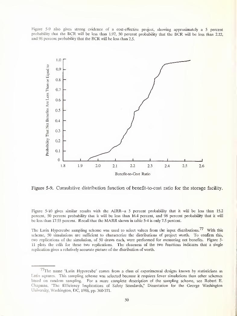
Figure 5-9 also gives strong evidence of a cost-effective project, showing approximately a 5 percent
probability that the BCR will be less than 1.97, 50 percent probability that the BCR will be less than 2.22,
and 98 percent probability that the BCR will be less than 2.5.
1.8 1.9 2.0 2.1 2.2 2.3 2.4 2.5 2.6
Benefit-to-Cost Ratio
Figure 5-9. Cumulative distribution function of benefit-to-cost ratio for the storage facility.
Figure 5-10 gives similar results with the AIRR—a 5 percent probability that it will be less than 15.2
percent, 50 percent probability that it will be less than 16.4 percent, and 98 percent probability that it will
be less than 17.55 percent. Recall that the MARR shown in table 5-4 is only 7.5 percent.
The Latin Hypercube sampling scheme was used to select values from the input distributions.^ With this
scheme, 50 simulations are sufficient to characterize the distributions of project worth. To confirm this,
two replications of the simulation, of 50 draws each, were performed for measuring net benefits. Figure 5-
11 plots the cdfs for these two replications. The closeness of the two functions indicates that a single
replication gives a relatively accurate picture of the distribution of worth.
' The name "Latin Hypercube" comes from a class of experimental designs known by statisticians as
Latin squares. This sampling scheme was selected because it requires fewer simulations than other schemes
based on random sampling. For a more complete description of the sampling scheme, see Robert E.
Chapman, "The Efficiency Implications of Safety Standards," Dissertation for the George Washington
University, Washington, DC, 1988, pp. 360-371.
50
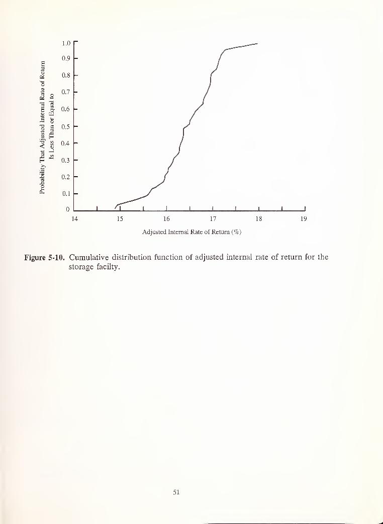
14 15 16 17 18 19
Adjusted Internal Rate of Return (%)
Figure 5-10. Cumulative distribution function of adjusted internal rate of return for the
storage facilty.
51

1500 2000 2500 3000 3500
Net Benefits ($1,000)
Figure 5-11. Two cumulative distribution functions of net benefits for the storage facility.
Replication 1 = solid line
Replication 2 = dotted line
5.4.2 Construction Contingency Simulation Example
Contingency analysis is routinely used by cost engineers in estimating the costs of construction projects. Acontingency is a cost element included in project cost estimation to cover costs that have some likelihood
of occurrence, but whose amounts cannot be predicated with certainty. By adding the contingency to the
line-item estimate of project cost, the cost engineer hopes to project the "most likely" final cost. Typical
uses of contingencies are to cover possible increases in material or labor costs beyond normal escalation,
unanticipated developments in applying a first-time technology, changes in project scope due to omission or
error, or unforeseen work disruptions from operating in a volatile foreign country.
Contingencies are often estimated simply as a percentage of the base estimate of project cost. Historical
data on the differences between actual and estimated costs for similar projects can be used to determine an
average percentage of underestimation (or overestimation). The percentage can apply to the overall project
or to specific elements of the project which are estimated separately. This simple approach is typical in
estimating costs of small projects. There is no distinction, however, between accounting for risk exposure
and risk attitude in the contingency estimate.
For a more complete listing of possible types of contingencies, see James J. Stevenson, Jr..
"Determining Meaningful Estimate Contingency," Cost Engineering, Vol. 26, No. 1, February 1984, pp. 35-41.
52
For large construction projects, a sophisticated risk-analysis technique based on simulations is oftenemployed in estimating contingencies. It provides decision makers with the probabilities of cost overruns(i.e., risk exposure) associated with every possible contingency markup in the relevant range. Thefollowing example from the Cost Engineers' Notebook illustrates how to use simulation to measure risk
, i- ••<• - • -79exposure when making a cost estimate for a specific construction project
Construction cost is being estimated for project X. It is expected to cost $140 million exclusive of
contingencies. Of the $140 million, $60 million are spent dollars or firm commitments. Being relatively
certain, they require no consideration for contingency. The other $80 million are uncertain and make upthe base on which the contingency is calculated.
The process for carrying out a "contingency/risk analysis" is as follows. Probability distributions are
generated for every activity that is deemed particularly uncertain. The distributions describe the percent of
estimated costs of these activities, where the midpoint is 100 percent of the estimated value. These data,
along with the estimated dollar costs of both certain and uncertain activities, are entered into a computersimulation package. It generates a probability distribution of the contingency percent of total project cost
and a graph that plots probability of cost overrun against contingency percent and amount.
Figure 5-12 shows how the probability of a cost overrun (i.e., risk exposure) varies with the contingencyadjustment for this construction project. To use this contingency/risk analysis to select a single cost
>,ocv
C
5U
90 80 70 60 50 40 30 20 10
i Greater Risk Lower Risk
Probability of Overrun (%)
16.0
14.0
12.8
11.0
8.9
8.0
6.4
4.8
3.2
1.6
0
-1.6
-3.2
20
18
16 n
14
12
t£10
~o
8 Dc
6 So
4U
2
0 11
-2
Figure 5-12*. Contingency /risk graph for construction project X.
*S. H. Zaheer, "Contingency and Capital Cost Estimates," Cost Engineers
Notebook, American Association of Cost Engineers, Morgantown, WV, March1983, p. 13.
79S. H. Zaheer, "Contingency and Capital Cost Estimates," Cost Engineers' Notebook, A-1.200, March
1983, American Association of Cost Engineers, pp. 1-14.
53

estimate, the decision maker considers risk exposure and risk attitude. Risk exposure, as indicated by the
rising probability of cost overrun, increases as the percent contingency markup goes down. Risk exposure
decreases as the percent contingency markup increases. Risk attitude enters when the decision maker
chooses a contingency amount, thereby establishing a probability of overrun that will be acceptable.
The risk neutral decision maker would choose the most likely cost estimate of $144 million, which includes
the $140 million without contingency plus a contingency of $4 million (0.05 • $80 million of uncertain
costs). That is, the vertical axis on the right side of the graph shows the most likely contingency percent
(where the probability of overrun is 50 percent) to be about 5 percent. This assumes an underlying
probability distribution which is symmetric.
A more risk averse decision maker might opt for a lower risk of overrun by choosing a larger contingency.
For example, if an overrun probability of only 20 percent were acceptable, the contingency would be $7.2
million (0.09 • $80 million), and the total cost estimate would be $147.2 million ($140 million plus $7.2
million contingency).
On the other hand, a risk taker might choose a relatively low contingency. For example, if an overrun
probability of 70 percent were acceptable, the contingency would be $1.6 million (0.02 • $80 million), and
the total cost estimate would be $141.6 million ($140 million plus $1.6 million contingency). Note that
figure 5-12 is really a cdf similar to that described in figure 3-2 with two exceptions. First, figure 5-12
has the axes reversed. The item whose distribution is being measured (contingency percent and amount) is
on the vertical axis instead of the horizontal axis, and the cumulative distribution measure (probability of
overrun) is on the horizontal axis. Second, the cdf in figure 5-12 measures cumulative probabilities of a
value being "greater than" instead of "less than," as in figure 3-2. Thus, for example, there would be about
a 35 percent probability of a cost overrun with a contingency of 7 percent. That is, there is a 35 percent
probability that the necessary contingency to avoid an overrun would be "greater than" 7 percent.^
5.4.3 Advantages and Disadvantages of Simulation
There are several advantages of the simulation technique applied to risk analysis. First, simulation works
with any kind of distribution of input variables, so it is not limited to certain classes of well-behaved
distributions.
Second, it can handle interdependencies between inputs. That is, where one input is related to another, the
two can be tied together. For example, if operating costs for the storage facility described earlier were
dependent on occupancy rates, then we would draw first a value for number of units occupied and then go
to the pdf on operating costs that includes the value of the occupancy rate that was already drawn. Thus
there would be several pdfs of operating costs that would map to every possible occupancy rate.
Third, simulation can be used in generating pdfs and cdfs for any of the economic measures described in
table 2-1.
Fourth, while it is true that the cdf describes only risk exposure, it also facilitates incorporation of risk
attitude by the decision maker in the decision process. That is, when the decision maker selects projects
on the basis of cdfs, inherent in that selection is an implicit assessment of risk attitude.
The disadvantage of simulation is that it requires many calculations, and is therefore practical only when
used with a computer.
°uFor additional information on contingency analysis, see Zaheer, "Contingency and Capital Cost
Estimates;" p. 13; J. R. Healy, "Contingency Funds Evaluation," American Association of Cost Engineers
Transactions , B-3, 1982; and M. W. Graf, "An Overview of Contingency Consideration," Cost Engineering ,
Vol. 26, No. 1, February 1984.
54

5.5 Mathematical/Analytical Technique
The mathematical/analytical (M/A) technique was developed by Hillier as a means of obtaining probability
functions for economic measures of worth without the repeated trials of simulation.81 The M/A technique
allows one to generate pdfs and cdfs of life-cycle costs, net benefits, and unadjusted internal rate-of-return
measures*82
Equations (5.5) and (5.6) show how to compute the aggregated, discounted mean and variance for the net
benefits measure of project worth. The input data are the mean and variance of net cash flows for each
year of the investment's study period.
N^NB = £ E(B
t- C
t)/(1 + i)1
, and (5.5)
t = 0
Na2NB = S Var(B
t- C
t)/(1 + i)2t
(5.6)
t = 0
where = the mean of net benefits,
° NB = tne variance of net benefits,
E(Bt
- C[) = the expected value (mean) of net benefits in time period t,
VAR(Bt
- Ct)= the variance of net benefits in time period t.
8^
By using the mean and variance of net benefits earned on the investment and the probability tables for the
normal distribution, pdfs and cdfs can be derived for net benefits of the investment. Also, the probability
of the investment yielding net benefits less than, equal to, or greater than zero (or some other specified
target value) can be computed directly.
The M/A technique requires that input values be normally distributed to generate pdfs and cdfs of the
measures of worth. Even without normal input distributions, however, the technique produces means and
variances of economic measures of worth. And these statistics by themselves can be highly useful.
The technique as applied here presumes independence in a single project's profitability over time.
Approaches to handling interdependence are treated in section 5.5.2.
81Hillier, "The Derivation of Probabilistic Information," p. 444.
82Park extended Hilher's model to develop a method for computing probability distributions of benefit-
cost ratios. See "Probabilistic Benefit-Cost Analysis," The Engineering Economist, Vol. 29, No. 2., 1983, pp.
83-100.
8^The notation for benefits and costs used in these equations is consistent with that of the formulas
in table A-l in appendix A.
55

5.5.1 Shopping Centers Example of M/A Technique
To illustrate the technique, a cdf is derived for net cash flows from an investment in a limited partnership
that is buying shopping centers.^ The minimum investment in the partnership is $5,000, so that is the
amount on which net cash flow returns will be estimated for making the economic evaluation. A 6-year
holding period is projected. Although fewer, or more, than 6 years may pass before the shopping centers
are sold and the proceeds distributed to investors, the brokerage house selling the partnerships will make a
market for the shares in the over-the-counter market. So we know with certainty that the investment can
be cashed in at the end of 6 years. Table 5-5 lists these and additional assumptions on which the case
illustration is based.
Note that net cash flows are not net of initial investment cost in this example. That is why we use the
term net cash flows here instead of net benefits. The approach followed in this case illustration is to (1)
apply Hilher's approach to the uncertain net cash flows and then (2) compare the final cdf of net cash
flows against the certain $5,000 investment cost to see how cost effective the shopping centers are likely
to be.
Table 5-5. Assumptions for the economic evaluation of the limited-partnership shopping
centers
1. $5,000 investment initial cost
2. 6-year holding period (study period)
3. 1987 (constant) dollars used in the analysis
4. 8% discount rate used
5. Cash flows (annual revenues minus annual costs) projections are normallydistributed in each period
6. Net cash flows are computed before taxes
7. Net cash flows are independent among years
8^This case illustration is based on data in part from a 1987 prospectus issued by a brokerage house
sponsoring a limited partnership for buying shopping centers. The prospectus is used only for the purpose
of helping to generate a realistic problem. The illustration is not intended to provide economic advice
about any particular investment opportunity in shopping centers.
56

Equations (5.7) and (5.8) are used to calculate the mean and standard deviation of present value net cashflows from the shopping centers over the 6-year study period. These equations differ slightly from eqs(5.5) and (5.6) in two ways. First n t
and at
2 do not incorporate investment costs, whereas E(Bt
- Ct)
andVar(B
t- C
t)would. Second, the apyc is computed directly by eq (5.8) rather than computing the variance
as in eq (5.6). Equations (5.9) and (5.10) are used to calculate the mean and standard deviations of netcash flows in each of the 6 years of the project study period.
N/WC = 2 (M 1 + i)*).
(5.7)
t = l
Napvc - (2 (a
t
2/(l + i)*))^
(5 g)
t = l
Kwhere nt
= 2 (CtsPts ), (5.9)
s = l
Ka
t= (S (C
ts - A*t)2Pts)
1/2. ^d (5.10)
s = l
where /^pvc = tne expected value of present value net cash
flows over the project holding period,
/it- the expected value of net cash flows in period t,
aPVC = tne standard deviation of the present value of net
cash flows over the project holding period,
= the variance of net cash flows in period t,
K = number of possible states of business success,
C(S= net cash flow associated with state s in period t, and
Pts= probability of state s in period t, and
at= the standard deviation of net cash flows in period t.
Four steps are described for deriving the pdf and cdf of the shopping centers. The first is to construct on
the basis of perceived uncertainty the net cash flow distributions for a $5,000 investment in the shopping
centers. Techniques for assigning probability to uncertain events have been developed elsewhere, so they
are not discussed here.^ Table 5-6 provides the probability distributions and means that describe
potential earnings of the shopping centers. Five states (s) of business success are hypothesized for the
^C. S. Spetzler and C. S. Stael von Holstein, "Probability Encoding in Decision Analysis," Readings in
Decision Analysis, pp. 403-427; A. Wilson, "Risk Analysis in Retail Store Design: A Case Study," Quality
and Profit in Building Design, edited by P. S. Brandon and J. A. Powell (London, England: E. & F. N.,
Spon, 1984); and Capen, "The Difficulty of Assessing Uncertainty," pp. 843-850.
57

Ucj4—
>
CJo
.a
Oho
a
oa
4-1
C
at-Ta
CCJ
s~3
V.
co
•fH-J—
J
3
H•4—1
.29
£O
HO
1H
•co
• rf
V-
>u
f..
co -u cu -u a> c/i c/i
in o o o mCm co in 00 <t
V> o VO 00 r- 1 oo oID •—
1
CM CM .—
i
oO •co-
CT\
in o o O in co-l£> —
i
CM n CMll
IDo CO o o oo in o in oV) CM VD o> COID
CJ) VD 00 o> o CM</> i—
i
.—
1
in o m o in om
Cm o CM o r~- oco .—1 CO 00co- •—
1
r-H .—1
O ooCfl O m o in o co-m •—
I
CN) CO CJ 1—
I
Cm ll
mn o O o O o a.to o m o in oU CO <f VD r-« cr>
•CO-
W»
Cm CD o m in OCO o VO oo</> r—
1
—1 —
i
lT oinin
n O in o in O co-•—
1
CM ro CM •—
I
Cm ll
-j
v> O o o o o a.O o in o oo OO <f U~) oo
co-
nco in I Pi O in in
CmCM o C J p-
n <—
i
co o VO coU co- CM H oo
inv) in in o in in •co-
co O CJ CM OCm ll
co
Ul o O o o o a.co m in o in mO CM co m r-.
CO-
i/l
cm CO O o o oCm
in m O o o mCM CM CO ^M VDO CO- '—
I
^1 oin<r
v) CO O O o O •co-
CM I—
1
CJ C J —
(
Cm ll
CM
VI o O o o o a.eg in in m m inO CM ro <t in vo
CO-
in
•M CO o o o OCm
o o o o oro VjO CM O CTi
C_> co- —1 i—
I
ooc^ in co-
•—
i
CM CO CM <—
i
Cm ll
o O o O O a?o o o o o
U CM co <J- m•CO-
to t—
1
CM OO in
58

group of shopping centers ranging from the least profitable state, s = 1, to the most profitable, s = 5.
Potential net cash flows (current earnings minus current expenses) are estimated for each of the 6 years
(t = 1 through 6) for all five states of success. The net cash flow (cts)
values are weighted by the
probabilities (Pts)
that those respective business conditions might occur. The Cts
and Pts
values define the
cash flow distributions for each year.
The following rationale was used in deriving the distributions for this case illustration. Based on current
shopping center earnings, the prospectus predicted an 8 percent return ($400 on the $5,000 investment) in
the first period (i.e., year). The dispersion of earnings about the mean (table 5-7) is based on uncertainty
about finding renters right away for shopping centers under new management. In the second period there
is a higher probability associated with a larger mean and a smaller variance than in the first period. It is
more likely that all of the space will be rented in the second year. Furthermore, two years are a short
enough time that the general partners feel confident in predicting high rental rates with greater certainty.
For periods t3 through [5, the mean continues to rise because rent escalation contracts call for increasing
rents (in constant dollar terms), while mortgage payments are fixed in current dollars (probably dropping in
constant dollar terms). The variance about the mean increases, however, because estimates become less
certain as the time horizon is extended. Resale proceeds have been coupled with annual net cash flows to
make all the values in the probability distribution for period 6 (col. Cgsin table 5-6) larger than those in
earlier periods. Resale (in constant dollar terms) is estimated at 1.2 to 2.4 times the $5,000 purchase price.
The second step is to calculate the mean, variance, and standard deviation of net cash flows for each of
the 6 years. The mean, shown as ^ ton the bottom line of table 5-6, is computed with eq (5.9). The
standard deviation, shown as aj- in table 5-7, is computed with eq (5.10).
The third step is to use eqs (5.7) and (5.8) to calculate the mean and standard deviation of the pdf of the
present value net cash flows over the 6 years. Substituting into the equations, we find for the pdf a mean
present value net cash flow of $8,015 and a standard deviation of $1,104, as shown below.
^pvc$400 $450 $500 $550 $600 $9,600
(1.08) 1 (1.08) 2 (1.08) 3 (1.08) A (1.08) 5 (1.08) 5
= $370.37 + $385.80 + $396.92 + $404.27 + $408.35 + $6,049.63
= $8,015, and
'pvc $16,000 $12,000 $17,500+ +
(1 .08) :
(1 .08)'
$23,750 $29,250 $2,916,000
(1.08) 6 (1.08) !
(1 .08) 1 0 (1.08) 12
1 / 2
= [$13,717.42 + $8,820.36 + $11,027.97 + $12,831.39
+ $13,548.41 + $1,157,983.70]1 / 2
[$1,217,929.30
$1 , 104.
1 / 2
59

Ifl CO
CO CD O o o O O o COCm Cm O o o -3 o oCN CN LO m LO in om in o in in o CN
CO CM CM CNI CM o rO CD ro ro r-M
NT) NO <—
i
LO5? CO-
CO- rO i—
'
ONto ro in LO on r-- CO
co </> CD <—
I
CMco-
II1
1
IIII
II II
CO lO m in CM co CO CNI CO
ro ^+ CO CD CDC-M Cm
CN CN o o O O OQ Q Q Q Q
CO o o o o CD O LO oa. LO m a.
CN r->
CO CN CO CN CNCO CN cm CD CN 00 CO CMu CO- "
</>
CO CO
CN CO
Cm CmCN o o o o o o o CN o LO o LO o o H
o o o o o c-H o CN CN o LOCM o o o o *—
I
m \Q rn CNa. co- a. •co-
CN CNI CM i tn IT) CTc CJ\
CO </> CO </> CNu i-H ij m <J>
u UCO II ll w 11 ll
x3Q CN Q LO
»HCO Q Q CN CO o LO LO CN
CM CN CN] IN 1) m cn CN K.\J
Cm (2 Cm
CM CNo o o o oCM o o o o cn o o o o oa. o o o o a. o o o o
1 o m n oCO
f—
\
r—
s
Q 10
CN <T -f\i in c^ CM CM* oO </> O C7\ CM CM OA
CO CO
<r
Pm o o <*CN o O o o o O NO o in o in in in in
o o o o o CM in CM CNI i'—
i
o o o o o <—
1
CM <o CM co-
a"1
</> ^! COCN] i vO in in M3 CM
CO Co- <—
1
to co- co-co- -a-
u Oll II ll ll
,—
1
CO lo o o o m CN H o m o in O CM
i—
i
CN CM <—
i
»M b *—
1
Cl ro CM '—
i
bCm
-1
b P-t b
CN <Nt—
j
o (3 Q OQ o o o
Q o1
LO LO lO in1
10 o O o o 10 CM CM CM CMi <r <D CM CM
o co- O </>
'/I 7)
u d)
jj
ct CM ro m ."j CM ro in4- u0"; c/3
(,()

The fourth and final step is to construct a pdf and cdf for the present value of net cash flows from the
shopping centers, and evaluate them in light of the $5,000 investment. To construct a pdf, ordinates from
a statistical table on normal curves are used to derive relative heights on the y axis for corresponding
present value net cash flows. However, ordinal values in statistical tables are given only for standardized z
values. Thus z values that correspond to specific dollar amounts must be available before corresponding
ordinates on the y axis can be found. Equation (5.11) shows the relationship between z and x, where x
represents net cash flow. Each z value measures the number of standard deviations that any given net cash
flow lies above or below the mean ($8,015).
z = (x - y)/a. (5.11)
Table 5-8 illustrates the derivation of the pdf with ordinate values. Arbitrary z values are selected (col. 1)
to establish the range of the distribution. Since 99.73 percent of all values in a normal distribution lie
within 3 standard deviations of the distribution mean, z values from 0 to 3.0 are chosen. The present value
net cash flow (x value) corresponding to each z value is computed for the range 3 standard deviations
below (col. 2) to 3 standard deviations above (col. 3) the mean. The ordinates (col. 4) for the
corresponding z values are taken from a statistical tabled Values for y are plotted in the same proportion
to one another as the ordinates in column 4. Figure 5-13 shows a smooth function drawn through these yplots to construct the pdf.
Table 5-8. Data for constructing probability density function of present value net cash flows
for shopping centers
Net Cash Flow Values ($)
z x = /z-zct x = /i+zo Ordinate at z
(1) (2) (3) (4)
0.0 8,015 8,015 .3989
0.5 7,463 8,567 .3521
1.0 6,911 9,119 .2420
1.5 6,359 9,671 .1295
2.0 5,807 10,223 .0540
2.5 5,255 10,775 .0175
3.0 4,703 11,327 .0044
86"The Normal Probability Function and Related Functions," Standard Mathematical Tables , 14th ed.,
edited by Samuel M. Selby, the Chemical Rubber Co.; Cleveland, Ohio, 1965, pp. 260-265. Note that x and
f(x) values in the Chemical Rubber Co. tables correspond respectively to z and ordinate values in this
report.
61

4.5 5.0 5.5 6.0 6.5 7.0 7.5 8.0 8.5 9.0 9.5 10.0 10.5 11.0 11.5
Present Value Net Cash Flows ($1,000)
Figure 5-13. Probability density function of present value net cash flows for shopping centers.
Note that the pdf by itself gives considerable information about the cost effectiveness of the shopping
centers. For example, visual inspection indicates that there is little area under the left tail of the pdf for
present value net cash flows less than $5,000, the amount that must be recovered to at least break even
with the initial investment. Thus we know immediately there is a low probability that the investment will
not at least break even. Furthermore, we can see directly that the most likely value of the net cash flows
is about $8,000.
The cdf in figure 5-14 is even more helpful, because it indicates the probability of being less than or just
equal to target levels of present value net cash flows over the entire range of possible outcomes.
Conversely, it can be used to determine the probability of exceeding target levels of present value net cash
flows.
Table 5-9 shows how the numbers are obtained for plotting the cdf. First we establish an arbitrary range
of present value net cash flows (col. 1) over which to plot the cdf. Since 99.73 percent of all values he
within 3 standard deviations of the mean, we can feel comfortable selecting a range of net cash flows
between ]i - 3a and \x + 3a. Looking back to table 5-8, columns 2 and 3 show a corresponding range of
net cash flow values from $4,703 to $11,327. For convenience we round to $4,000 and $12,000 with $1,000
intervals. Column 1 in table 5-9 shows the present value net cash flow amounts for which the cdf is
constructed.
A z value is computed in table 5.9 (col. 2) for every net cash flow value (col. 1) using eq (5.11). This is
necessary because curve areas in statistical tables are given only for standardized z values. The associated
normal curve areas for z values in column 2 are listed in column 3 of table 5-9.^ The area value
8 'The normal curve areas were found in table 10, "Table of Areas of the Normal Curve," Tables for
Statisticians, by Herbert Arkin and Raymond R. Colton (New York, New York: Barnes and Noble, 1950), p.
114.
62
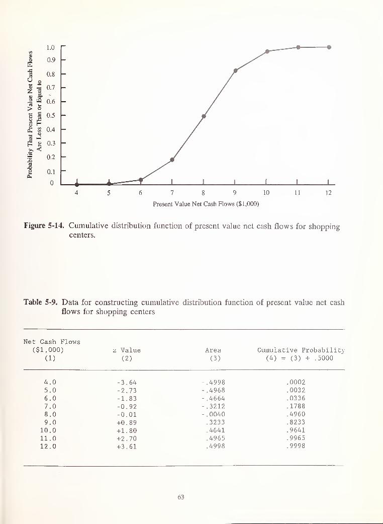
1.0CO
0.9OEJ3
U.ou QNet
30 7
313
a* 0 6
> Q
c s r\ <;U.jr"
tou Hu.
d.COto 0.4
03
D
0.3
>, <0.2
bab
1 0.1
0
7 8 9 10
Present Value Net Cash Rows ($1,000)
Figure 5-14. Cumulative distribution function of present value net cash flows for shopping
centers.
Table 5-9. Data for constructing cumulative distribution function of present value net cash
flows for shopping centers
Net Cash Flows
1 ,000) z Value Area Cumulative P
(1) (2) (3) (4) = (3)
4.0 -3.64 - .4998 .0002
5.0 -2.73 - .4968 .0032
6.0 -1.83 - .4664 .0336
7.0 -0.92 - .3212 . 1788
8.0 -0.01 - .0040 .4960
9.0 +0.89 .3233 .8233
10.0 +1.80 .4641 .9641
11.0 +2.70 .4965 .9965
12.0 +3.61 .4998 .9998
63

describes what percent of total area under the pdf lies between the mean and some specified number of
standard deviations (z value) to the right (positive area value) or left (negative area value). Theprobability that net cash flows will be less than or equal to any given target value of PVC in column 1 is
the area under the pdf to the left of the target value. To find the cumulative probability (col. 4) at any
given present value net cash flow, the area of the corresponding z value is added to 0.5000.
Let us first use table 5-9 to evaluate the likelihood that our $5,000 investment will at least break even.
The area under the normal curve to the left of $5,000 is found as follows: The value of z = -2.73 (i.e.,
($5,000 - $8,015)/$1,104). The area under the normal curve between the mean and the z value of -2.73 is
0.4968. The difference between this area and the total area to the left of the mean is 0.0032 (i.e., 0.5000-
0.4968). Thus, given the data used in the analysis, there is less than a 1 percent chance that the
shopping centers would not at least break even. Given the extremely low probability of a loss, all but the
most risk-averse decision makers would likely accept this investment unless other higher-return alternatives
with similar or less risk were competing for limited budget funds.
We can also examine the cdf to determine probabilities that the investment will achieve various degrees of
profitability or loss. For example, we find about a 50 percent probability that returns would be less than
$8,000 ($3,000 profit) and about a 97 percent probability that returns would be less than $10,000 ($5,000)
profit.
5.5.2 Advantages and Disadvantages of M/A Technique
A major advantage of the M/A technique is that means and variances (and therefore pdfs and cdfs) of
project worth can be generated directly by hand calculations without repeated simulations on a computer.
Thus risk exposure can be determined without the use of a computer.
Another advantage is that implicit incorporation of risk attitude into the selection process is facilitated
when the decision maker selects a project based on cdfs.
A disadvantage of the M/A technique is that it presumes that the underlying probability distributions
associated with the inputs are normally distributed. This condition is necessary to generate precise
probability statements about the measure of worth. However, Hillier has suggested that the subjective
probability distributions analysts tend to generate in describing uncertain events are often symmetrical and
resemble normal distributions. Furthermore, even where the distributions are not normal, the mean and
variance of the measure of worth, as computed by eqs (5.5) and (5.6), will still be accurate and provide
helpful information in evaluating alternative investments.
A possible disadvantage with the M/A technique is in specifying and calculating the impacts of
interdependence among a single project's measures of worth over time. For example, the level of
interdependence among NB in, let us say, years 1, 2, and 3 might range from total independence (zero
correlation among NB in different years) to total interdependence (perfect correlation among NB in
different years).
One approach to handling interdependence is to use sensitivity analysis-calculate the variance first with
the assumption of zero correlation and then with the assumption of perfect correlation. A more accurate
approach is to assume that net benefits in some years are related and in other years they are not. Hillier
presents a mathematical model for calculating the mean and standard deviation under conditions of varying
interdependence.^
88Hillier, "The Derivation of Probabilistic Information," p. 446.
^F. Hillier, "The Evaluation of Risky Interrelated Investments," Studies in Mathematical and
Managerial Economics, ed. by Henri Theil, North-Holland, Amsterdam, 1969.
(.4

A second interdependence issue arises when evaluating interrelated projects. The economic worth of one
project may vary as a function of the worth of competing or complementary projects. For example, the
returns from a given investment may be correlated to returns on other investments in a group of projects
because all of the projects are affected by common factors. Hillier has developed techniques for evaluating
large, risky, interrelated investments.^
Another disadvantage of the M/A technique is that the input distributions in each period must be of the
measure of economic worth. That is, the uncertainty expressed in the input distributions pertains only to
the final measure of project worth for that period. Thus for the NB measure, for example, the distribution
in each period would be of NB. This means that the analyst would already have had to determine how all
of the uncertain factors that affect benefits and costs combined in a given period to make that period's
NB distribution. The simulation method, on the other hand, accommodates separate distributions for each of
the uncertain inputs and provides for then systematic combining to form a final distribution of the measure
of project worth. It should be noted, however, that in the simulation approach, the input variables are all
discounted to present or annual values, whereas in the M/A approach, there is a separate distribution for
each period in the project's time horizon. Thus the latter has more opportunity for fine tuning the
estimated project performance from period to period.
5.53 M/A Technique Used with the CEF and RADR Techniques
The M/A technique can be used in conjunction with the risk-adjusted discount rate or certainty equivalent
technique in computing NB. The uncertainty associated with the variables used to compute NB period-by-
period is captured in the probability distributions of net cash flows. Thus risk exposure is indicated by the
mean and variance of NB and by the pdf and cdf generated from those statistics. Risk attitude, on the
other hand, is incorporated exclusively in the CEF or RADR adjustment to NB.
When using the RADR technique, the RADR value, as defined in eq (4.1), substitutes for discount rate "i" in
eq (5.5). Equation (5.6) is used as shown.9 -*- The AR2 component of the RADR value should adjust for risk
attitude only. Thus the more risk averse is the decision maker, the higher will be the RADR valued
Note that, if the RADR adjusts for risk exposure while using the M/A technique, there will be an
overadjustment for risk exposure.
The advantage of a joint M/A and RADR analysis over using the M/A or simulation technique alone is that
it treats risk attitude in a formal manner. Typically the mean and standard deviation (and pdf and cdf)
reflect only risk exposure, and the decision maker has to make a subjective determination of risk attitude
when considering each project alternative. When using the techniques jointly, on the other hand, the
distributions already have risk attitude incorporated in them. That is, the NB values have been adjusted by
the RADR to reflect, in effect, their certainty equivalent or utility values. Thus the decision maker whose
objective function is to maximize the expected value of utility simply chooses the project with the higher
expected value of adjusted net benefits.
If decision makers are not comfortable with a choice based on expected values adjusted for risk attitude,
additional selection rules might be used in determining which project is preferred after applying eqs (5.5)
and (5.6). Where the pdf and cdf show clear stochastic dominance, they can be the guide to project choice.
Where stochastic dominance is not obvious, the preferred project might be the one with the lower
coefficient of variation (sec. 5.2).
90Ibid.
91The RADR and CEF adjustments apply to the mean, but not to the variance, when used with the
M/A technique.
92rhis presumes that benefit streams are being discounted. As discussed in section 4.4, if cost streams
are being discounted, AR2 is adjusted downwards to compensate for a risk averse attitude.
65

When using the certainty equivalent technique (sec. 4.5) with the M/A technique, the CEFtwould be
inserted into eq (5.5) as a multiplicative factor times E(Bt
- Ct ).
Equation (5.6) is used as shown. A risk-
free rate of interest would be used for discounting.^ in this case, CEFtshould adjust for risk attitude
only. Thus, the more risk averse is the decision maker, the lower would be the CEFf and the lower would
be the mean of NB. Once again note that, if the certainty equivalent technique also adjusts for risk
exposure while using the M/A technique, there will be an overadjustment for risk exposure.
The same selection rules discussed for the RADR determining the preferred project are applicable to the
certainty equivalent technique. And, as is the case with the RADR technique, when used with the M/Atechnique, the certainty equivalent technique provides a formal treatment of risk attitude. Thus the
decision maker whose objective function is to maximize the expected value of utility might simply choose
the project with the higher expected value of adjusted net benefits.
5.6 Other Techniques
Additional techniques for evaluating investments, which are based on distributions and include utility
considerations in the decision-making process, are gaining increased attention in the building field. The
two techniques described briefly here are used to evaluate the risk and return of combinations or
portfolios of projects in which interactions among the projects affect the overall riskiness of the portfolio,
and to determine what the expected return of an individual asset should be, given its risk.
5.6.1 Portfolio Analysis
Portfolio analysis is a technique used to seek the combination of assets with the maximum return for any
given degree of risk (i.e., variance of the return), or the minimum risk for any given rate of return.^ By
diversifying its assets so that returns are not perfectly positively correlated, a firm's overall investment
risk can be reduced. The risk reduction from this diversification of assets is called the portfolio effect.
Portfolio theory was originally developed for the analysis of stocks. The model has been extended,
however, to the analysis of other assets. The evaluation of building investments seems a logical application
of portfolio theory. Yet few applied efforts have been made. One reason is that it is difficult to get data
to measure the correlation of building investments.
Another reason portfolio analysis is not applied frequently to building investments is that they involve large
chunks of capital, large and lumpy chunks of real estate, cumbersome markets, lengthy transaction times,
and large transaction costs. This is certainly a more complex market environment than the New York Stock
Exchange provides, for example, to an investor accumulating and managing a portfolio of stocks.
An academic study of portfolio analysis in construction is available in Vegara's thesis.^ It combines
probabilistic estimating, portfolio theory, and utility theory in the development of models for helping
construction firms select an optimal mix of new projects.
y:5Note that it is appropriate to use risk-free rates of interest for discounting whenever risk is being
accounted for by some means other than the RADR.
^For a LCC analysis, the more risk averse is the decision maker, the higher would be the CEFt
.
9^For the landmark treatment of portfolio analysis, see Harry Markowitz, Portfolio Selection: Efficient
Diversification of Investment (New York, New York: John Wiley and Sons, 1959).
™J. A. Vegara, "Probabilistic Estimating and Applications of Portfolio Theory in Construction," Ph.D.
Thesis, Graduate College of the University of Illinois at Urbana-Champaign, Urbana, Illinois, 1977.
66
5.6.2 Capital Asset Pricing Model
The Capital Asset Pricing Model (CAPM), the best known model of risk and return among asset pricing
models, is an extension of portfolio theory.97 It explains how an asset should be priced based on the
additional risk it will add to the risk of a market portfolio of assets. Said another way, it indicates whatthe return on an asset should be, based on that asset's risk.
Two types of risk are attributed to any investment in an asset. One is unsystematic risk; that is, risk
associated with random events, such as fires and strikes, that are unique to the investment. The other is
systematic risk (also called market risk) resulting from market variations to which all investments are
subjected.9^
Unsystematic risk can be eliminated with a diversified portfolio, but systematic risk cannot. The systematic
risk of a given asset is a function of how sensitive its return is to changes in market conditions. This
sensitivity to market conditions is measured by "beta." The beta coefficient is measured as the covariance
of the asset's returns with the market portfolio's returns. According to CAPM, an asset's beta measures
the risk that is compensated in the market place. Thus higher returns are not predicated for higher
unsystematic risk. An asset with a beta of 1.0 has average market risk and, therefore, one would expect an
average return for it. A beta below 1.0 indicates proportionately less-than-average market risk and
therefore a lower return. And a beta above 1.0 indicates proportionately more-than-average market risk
and therefore a higher return.
Risk and return relationships can be specified using CAPM. Once the risk/return relationship is defined,
the expected rate of return on an asset can be estimated based on its systematic risk as defined by beta.
The return on an asset should equal the risk-free rate of return plus a risk premium in proportion to the
asset's beta. An asset with an estimated return higher than the expected return based on its beta would be
a "good buy." Over time, however, increased demand for it will raise its price and lower its relative
return in a perfect market until the estimated return is in line with the asset's beta.
Portfolio analysis and the CAPM show promise theoretically for the evaluation of building investments. The
data needed to apply these techniques, however, are not available. Estimating the beta for a real estate
investment, for example, is much more complicated than for a stock. Thus widespread application of these
techniques awaits additional research.
97For the landmark treatment of the Capital Asset Pricing Model, see W. F. Sharpe, "Capital Asset
Prices: A Theory of Market Equilibrium Under Conditions of Risk," Journal of Finance , Vol. 19, No. 4,
September 1964.
^Examples of events that affect market risk are interest rate changes, war, and economic expansion
and contraction.
99For a treatment of CAPM and other asset pricing theories, see Russell J. Fuller, Capital Asset
Pricing Theories-Evolution and New Frontiers, Monograph No. 12, The Financial'Analysts Research
Foundation, Charlottesville, Virginia, 1981.
67

6. CONCLUSIONS
If it can be agreed that better decisions come from more complete information, then accounting for
uncertainty and risk will enhance decision making. Yet there is no "best" technique for handling
uncertainty and risk in evaluating every investment. What is best will depend on circumstances of the
organization. The analyst and decision maker should consider the following items of information before
selecting a technique for a given investment problem.
First, the level of resources must be assessed. How much time is available to evaluate the project? Howmuch money is available for staff and computer support? Does the staff have the technical capability to
apply all of the techniques? For example, can they derive utility functions from inferred risk attitudes and
develop probability distributions for uncertain variables? And finally, are computer software and hardware
available for applying all of the techniques? By asking these questions, the set of feasible techniques
(where feasibility depends on resource availability) can be defined.
Second, the particular audience that will use the analysis must be identified, and their reactions to the
techniques should be considered. Has executive judgment and intuition been successful in the past? Will
the management team understand the information generated from applying the techniques? Will they
accept the different types of information produced by the techniques? If the chief executive officer has
been choosing profitable projects on the basis of personal judgments and deterministic, single-value
estimates of project worth, for example, the analyst who presents cumulative distribution functions using
the simulation technique will probably have little influence.
Third, the approximate size of the investment relative to the institution's budget or portfolio of other
investments should be taken into account. For example, if the investment to be analyzed were small
relative to the total portfolio, and would affect total profitability only slightly if it yielded a poor return,
then a sophisticated approach to risk analysis such as the mathematical/analytical technique would not be
needed. On the other hand, if the investment were relatively large, and a poor return could bankrupt the
institution, then a sophisticated technique might be needed.
Fourth, risk attitude should be considered in choosing a technique. If the decision maker were risk neutral,
for example, decisions could be made on the basis of maximizing net benefits instead of utility, and the
procedure to account for risk attitude would be unnecessary. If the decision maker were very risk averse
or a risk taker, on the other hand, it becomes appropriate to use techniques that can adjust for risk
attitude, such as decision analysis, the risk adjusted discount rate, and certainty equivalent technique.
Table 6-1 is a quick-reference guide to the 10 techniques described in this report for treating uncertainty
and risk. Column 1 indicates the form in which input data are accepted for each technique. The
possibilities include single values (S), multiple values (M), and probability distributions (D). For example,
the technique "conservative benefit and cost estimating" is shown to require single-value data inputs,
whereas the simulation technique requires probability distributions. On the other hand, the risk-adjusted
discount rate or certainty equivalent technique can be used with either single values or probability
distributions.
Column 2 indicates the form in which the measure of project worth is expressed. It can be expressed as a
single value (S), multiple values (M), or distribution of values (D). Input estimation using expected values
displays the measure of worth as a single value, for example, whereas the mathematical/analytical approach
yields a cumulative distribution of worth values.
Column 3 treats risk exposure. Explicit (Ex) consideration means that a numerical adjustment for or
graphical measure of risk exposure is provided by the technique. The cumulative distribution of project
worth given by the simulation and mathematical/analytical techniques are explicit measures of risk
exposure. An implicit (Im) treatment considers risk exposure, but does not treat it quantitatively or
graphically. Sensitivity analysis, for example, suggests a possible range of output values, and thereby
implies something about risk exposure, but does not quantify that risk exposure.
OS

Table 6-1. Characteristics of techniques for treating uncertainty and risk
(1) (2) (3) (4)
Technique(S)
VnTm n "Fi UI 111 w ±.
InputData(M) (D) (S)
Phttti n "F1 U L 111 KJ J-
Measureof Worth
(M) (D)
RiskExposure(Ex) dm)
Pnn c i Hpt
RiskAttitudeCEx) (Im)
ConservativeBenefit andCost Estimating
k * •k
BreakevenAnalysis 3
k k k
Sensitivity-Analysis
* k k
Risk-Adj us tedDiscount Rateb
* k k -k k k
CertaintyEquivalent*3
k A * k k k *
Input EstimationUsing ExpectedValues 0
•k *
Mean-Variance/Coefficient ofVariation
k k k k
Decis ionAnalysis
k * k k k
Simulation •k k k *
Mathematical/ k k *
Analytical
09

Table 6-1 (continued)
(S_) = single value for each data (S) = single-value measure of worthinput (M) = multiple-value measure of worth
(M) = multiple values for each (D) = distribution of measure of worthdata input
(D.) = distribution of values for
each data input(Ex) = explicit, numerical measure of risk(Im) = implicit consideration of risk
a Breakeven analysis solves for the value of the uncertain input value thatwill just make the investment break even (e.g., NB = 0 , BCR = 1.0, orAIRR = MARR) . Thus the economic measure of worth would be a single value.
b Risk-adjusted discount rate and certainty equivalent techniques have bothsingle values and distributions of values indicated for the form of datainput and for the form of measure of worth. Distributions are citedbecause both techniques can be used with the mathematical/analyticaltechnique
.
c Input estimation using expected values does not treat risk exposure or
risk attitude. Expected values are computed only for inputs, yielding no
information in the single-value measure of worth to help the decision makerconsider even implicitly risk attitude.
Column 4 treats risk attitude. Explicit consideration occurs when a numerical adjustment is made for risk
attitude in project evaluation. Using utility functions with decision analysis is one example. Implicit
treatment considers risk attitude, but provides no measure of it in project evaluation. For example, if a
cumulative distribution function of project worth is constructed through simulation, implicit in the decision
based on that function is the decision maker's attitude towards risk. That is, a risk-averse decision maker
might very well make a different decision than a risk taker, given the same profile of risk exposure.
Note that the risk-adjusted discount rate and certainty equivalent techniques can be applied to treat risk
exposure and attitude either explicitly or implicitly.
Once the questions asked earlier about resources, management acceptance, and risk attitude have been
answered, table 6-1 can help decision makers or analysts select the appropriate technique. Suppose, for
example, a decision maker wants to know the range of possible AIRRs an investment might take and at
least enough information for the implicit consideration of risk exposure and risk attitude. Furthermore,
assume that the decision maker is uncomfortable with the process of generating probability functions of
uncertain events and prefers deterministic over non-deterministic answers. Looking at table 6-1, the single
technique that satisfies these conditions is sensitivity analysis. Multiple (but deterministic) AIRR values are
obtained, and information in the form of an array of possible AIRR values is given that helps the decision
maker consider risk exposure and attitude implicitly in making a decision. Any other technique that would
meet the criteria for this decision maker would violate the constraint that probability functions not be
used.
70

Over half of the techniques in table 6-1 use probability distributions in displaying the measure of project
worth. Yet these techniques are rarely used in the building community. Why are they not more common?It is not due to lack of research. An early treatment by Hillier
1^ demonstrated mathematical/analytical101 109
techniques for measurmg risk exposure. And Pohquenlul and Hertz1^ described in detail the application of
the simulation technique. More recent works in capital budgeting^ and engineering economics ^ continue
to explain the techniques. In addition, commercial software is available to perform these analyses on
widely-available microcomputers.^5
One author explains the paradoxical low level of use historically in the following description of the non-
deterministic approach in LCC analysis:^6
"... its variable output is harder to understand, it is more costly to set up and operate, and its answer is
often unwelcome. Few managers want to tell their supervisor or their customer that a project is risky or
an estimate uncertain. Thus, although it is possible to construct probabilistic models that are intellectually
satisfying and mathematically rigorous, most LCC models are deterministic."
Although this explanation is probably correct for the past, new evidence suggests that techniques for risk
analysis are of increasing interest to the building community and will become increasingly common in the
economic evaluation of buildings and building components. First, increasing education in these techniques
will yield practitioners that will understand and want to use them in building evaluations. Second, the
increased availability, decreased cost, and better understanding of computers and applied software will make
computations much easier. Third, managers are increasingly better educated in advanced analysis techniques
and are requesting risk analysis as a routine part of economic evaluations. And fourth, technical societies
such as the American Society for Testing and Materials are encouraging the development of standard
methods for measuring the risk associated with economic measures applied to building decisions.
100Hilher, "The Derivation of Probabilistic Information," 1963.
1 ni±u±Pohquen, Risk Analysis in Project Appraisal, 1970.
102Hertz, "Risk Analysis in Capital Investments," 1964.
•^Weston and Brigham, Managerial Finance, 1981.
lO^Newnan, Engineering Economic Analysis, 1980.
105One example of software is "Supertree™ Decision Analysis Software," from SDG Decisions Systems,
Menlo Park, California.
106Robert M. Seldon, Life-Cycle Costing: A Better Method of Government Procurement (Boulder,
Colorado: Westview Press, 1979), p. 163.
71


APPENDIX A. Formulas for Calculating Economic Measures
Table A-l. Formulas useful for measuring the economic worth ofbuilding investments 3
To Measure Use This Formula
Life-Cycle CostN
LCC = 2t=0
(C t- B t )/(1 + i) fc
(1)
Net Benefits 15
N
NB = X
t=0
(B t- C t )/(1 + i)
1
(2)
Benefit- to-Cost RatioN
BCR = S
t=l
(Bt
- C t )/(1 + i)* /C 0 (3)
Adjusted Internal Rateof Return (AIRR)
Find the AIRR Value for which
N
S (Bt- C t )(l + r t )
N_t /(l + AIRR) N
t=l
Solve directly
AIRR = -1 + (TV/CD )
1/N, or
AIRR = -1 + (1 + r)(BCR) 1/N,where
r is a constant, and r = I.
-Co =0, or (4)
(5)
(6)
a Only present value formulas are shown in table A-l. Annual value measures
could also be used.
b When the main effect of a project is to reduce costs, Ct
in formulas 2-7
will be negative. Thus there will be a cost reduction or savings resulting in
a positive value. (The minus sign coupled with a negative value yields a
positive value.) These savings are added to any positive benefits the project
might have over the alternative. When cost reductions dominate, the net
benefits measure is called the net savings measure, and the benefit- to-cost
ratio is called the savings- to -investment ratio.
73

Table A-l (continued)
SYMBOLS
N = total number of discounting periods in the study period,
Ct= costs associated with a given investment alternative in time period t,
Bt
= benefits (e.g., resale value) associated with a given investmentalternative in time period t,
i = discount rate for the period considered,
B t= benefits (including resale values) in time period t for the projectbeing evaluated less the benefits in time period t of a mutuallyexclusive alternative against which it is being compared,
Cfc
= costs in time period t for the project being evaluated less the costsin time period t of a mutually exclusive alternative against which it
is being compared,
C Q= initial project costs, net any initial benefits, for the project being
evaluated less initial project costs, net of any initial benefits, for
a mutually exclusive alternative against which it is being compared,
r t= reinvestment rate in time period t, and
N
TV = terminal value = 2 (Bt- C
t)(l + r
t )N_fc
t=l
74

APPENDIX B. Constructing a Utility Function
This appendix explains one approach107 to the construction of utilityfunctions. The approach derives the utility function directly throughquestions to a decision maker about willingness to trade guaranteed sums forlarger, uncertain sums. The appendix also presents the data on which thethree utility functions in figure 3-7 are based. Figure B-l is used here to
explain the derivation of the three functions in figure 3-7. Figure B-l is
exactly like figure 3-7, except that the points through which the curves werefitted are shown in figure B-l.
The function in figure B-l that bends over to the right indicates a riskaverse (RA) decision maker. The RA function is used to explain the process of
constructing a utility function. The steps taken to construct it were asfollows
:
(1) Two arbitrary incomes were selected. The decision maker chose $0 and$100,000. Then the decision maker was asked to assign arbitrary utilityvalues (U) to these two incomes. They were as follows:
U($100,000) = 70 U($0) = 0
(2) The decision maker was then asked to choose the amount of money(certainty equivalent) which he would be indifferent to receiving whencompared to the following lottery:
.50 U($100,000) + 0.50 U($0)
The decision maker chose $25,000, half the $50,000 expected value of the
lottery. By substitution we solve for the corresponding utility value as
follows
:
U($25,000) = 0.50(70) + 0.50(0) = 35
(3) Using the U($25,000) as a known value, another point is experimentally
determined by finding the certainty equivalent which the decision maker would
be indifferent to receiving when compared to the following lottery:
0.50 U($25,000) + 0.50 U($0)
The choice was $5,000, considerably less than the $12,500 expected value of
the lottery. By substitution we find the corresponding utility value of
$5,000 as follows:
U($5,000) = 0.50(35) + 0.50(0) = 17.5
107Examples of other approaches to constructing utility functions are to base utility measures (1) on
observations of individual or firm behavior in practice and (2) on recorded behavior in games of chance
designed to test risk attitude.
75

(4) To find utility values for levels of income greater than $25,000,alternative lotteries are posed that use the known utility values of $25,000and $100,000. For example, the decision maker was asked to choose the amountof money which he would be indifferent to receiving when compared tothe following lottery:
0.90 U($100,000) + 0.10 U($25,000)
The decision maker chose $70,000, compared to an expected value of $92,500.By substitution we solve for the corresponding utility value as follows:
U($70,000) = 0.90(70) + 0.10(35) = 66.5
(5) When asked to choose a value for the certainty equivalent of thislottery
,
0.75 U($70,000) + 0.25 U($25,000),
the decision maker chose $50,000, compared to an expected value of $58,750.By substitution we find the corresponding utility value as follows:
U($50,000) = 0.75(66.5) + 0.25(35) = 58.6
(6) To find a point in the range where the decision maker could lose money, a
loss situation was introduced into the lottery. The decision maker was askedto find the probabilities of outcomes which would make him indifferent betweenthe following lottery and the certain equivalent from doing nothing.
PU • ($5,000) + (1-P) • U(-$5,000) = U($0),
where P and (1-P) sum to 1.0.
The decision maker assigned to P the probability 0.70 and to (1-P) the
probability 0.30. Substituting known values for U($5,000) and U($0) yieldedthe utility of losing $5,000; i.e.,
0.70(17.5) + (.30) • U(-$5,000) = 0
U(-$5,000) = -(. 70(17. 5))/0. 30
= -40.8
To complete the process of constructing the risk averse utility function, a
curve was statistically "fitted" through the combination of points selectedarbitrarily ($0, 0; $100,000, 70) and experimentally ($25,000, 35; $5,000,17.5; $70,000, 66.5; $50,000, 58.6; and -$5,000, -40.8), as shown in functionRA in figure B-1. 108 A curve- fitting routine from DATAPLOT , a computer programdeveloped at the National Institute of Standards and Technology, was used to
establish the utility function. The risk taking (RT) and risk neutral (RN)
functions in figure B-l were constructed with the same routine, using the datashown in table B-l.
109
108por additional information on how to construct utility functions, see Berger, Statistical Decision
Theory and Bayesian Analysis, pp. 46-70, and Ronald A. Howard, "Risk Preference," Readings in Decision
Analysis , ed. by Ronald Howard et al. (Menlo Park, California: SRI International, 1977,
pp. 431-465.
^Robert e. Chapman of the National Institute of Standards and Technology ran DATAPLOT to
construct the three utility functions.
76

T 100
.RN
/
J- -50
Figure B-l. Three types of risk attitude: Data and fitted functions.
RN = risk neutral
RA = risk averse
RT = risk taking
Table B-l. Data for plotting utility functions
Risk Taker Risk Neutral
Thousands Utility Thousands Utilityof $ of $
-40 -10 0 -20 -25.0-30 -7 5 -10 -17.5-15 -5 0 -5 -7.5
0 0 0 0 0.015 5 0 5 7.5
35 10 0 15 15.0
50 20 0 20 25.0
60 22 5 25 35.0
65 30 0 40 47.5
70 35 0
80 42 5
85 50 0
77


BIBLIOGRAPHY
American Society for Testing and Materials. Annual Book of Standards , Vol. 04.07 (Philadelphia, Pennsylvania:
ASTM, 1987).
American Society of Heating, Refrigerating and Air-Conditioning Engineers, Inc. "Life-Cycle Costing," ASHRAEHandbook, Chapter 42 (Atlanta, Georgia: ASHRAE, 1984).
Arkin, Herbert and Colton, Raymond R. "Table of Areas of the Normal Curve," Tables for Statisticians (NewYork, New York: Barnes and Noble, 1950).
Arrow, Kenneth J. and Lind, Robert C. "Uncertainty and the Evaluation of Public Investment Decisions," TheAmerican Economic Review, Vol. LX, No. 3, June 1970.
Au, Tung and Au, T. P. Engineering Economics for Capital Investment Analysis (Boston, Massachusetts: Allyn
and Bacon, Inc., 1983).
Au, T., Shane, Richard M., Hoel, Lester A. Fundamentals of Systems Engineering: Probability Models (Reading,
Massachusetts: Addison-Wesley Publishing Company, 1972).
Baumol, William. Economic Theory and Operations Analysis, Fourth Edition (Englewood Cliffs, New Jersey:
Prentice-Hall, Inc., 1977).
Berger, James O. Statistical Decision Theory and Bayesian Analysis, 2nd Edition (New York, New York:
Springer-Verlag, 1985).
Capen, E. C. "The Difficulty of Assessing Uncertainty," Journal of Petroleum Technology, August 1976.
Chapman, Robert E. "The Efficiency Implications of Safety Standards." Dissertation for the George Washington
University, Washington, DC, 1988.
Chemical Rubber Company. "The Normal Probability Function and Related Functions," Standard Mathematical
Tables, 14 ed., edited by Samuel M. Selby, Cleveland, Ohio, 1965.
Clark, J. J., Hindelang, T. J., and Pritchard, R. E. Capital Budgeting: Planning and Control of Capital
Expenditures (Englewood Cliffs, New Jersey: Prentice-Hall, Inc., 1984).
Curran, Michael W. "Range Estimating for Plaudits and Profits," Baltimore Engineer , April 1986.
Dell-Isolla, Alphonse and Kirk, Stephen J. Life-Cycle Costing for Design Professionals (New York, New York:
McGraw-Hill, 1981).
Farragher, Edward J. "Capital Budgeting Practices of Non-Industrial Firms, The Engineering Economist, Vol. 31,
No. 4, Summer 1986.
Fellner, W. Probability and Profit (Homewood, Illinois: Richard D. Irwin, Inc., 1965).
Flanagan, Roger; Kendell, Adrian; Norman, George; and Robinson, Graham. "Life-Cycle Costing and Risk
Management," CIB Proceedings of the Fourth International Symposium on Building Economics, Danish
Building Research Institute, Copenhagen, 1987.
Friedman, Milton and Savage, L. J. "The Utility Analysis of Choices Involving Risk," Readings in Price Theory
(Homewood, Illinois: Richard D. Irwin, Inc., 1952).
79

Fuller, Russell J. Capital Asset Pricing Theories-Evolution and New Frontiers, monograph No. 12, The Financial
Analysts Research Foundation, Charlottesville, Virginia, 1981.
Graf, M. W. "An Overview of Contingency Consideration," Cost Engineering, Vol. 26, No. 1, February 1984.
Gurnani, C. "Capital Budgeting: Theory and Practice," The Engineering Economist, Vol. 30, No. 1, Fall 1984.
Healy, J. R. "Contingency Funds Evaluation," American Association of Cost Engineers Transactions, B-3, 1982.
Hendrickson, Robert G. A Survey of Sensitivity Analysis Methodology, National Bureau of Standards Interagency
Report 84-2814, February 1984.
Hertz, D. "Risk Analysis in Capital Investment," Harvard Business Review, January 1964.
Hillier, F. "The Derivation of Probabilistic Information for the Evaluation of Risky Investments," Management
Science, April 1963.
Hillier, F. "The Evaluation of Risky Interrelated Investments," Studies in Mathematical and Managerial
Economics, ed. by Henri Theil, North-Holland, Amsterdam, 1969.
Hirshleifer, Jack and Shapiro, David L. "The Treatment of Risk and Uncertainty," ed. Robert Haveman and Julius
Margolis, 2nd ed., Public Expenditure and Policy Analysis, 1977.
Holstein, C. S. von. "A Tutorial in Decision Analysis," Readings in Decision Analysis, ed. by Ronald Howard et
al. (Menlo Park, California: SRI International, 1977).
Howard, Ronald A. "Risk Preference," Readings in Decision Analysis , ed. by Ronald Howard et al. (Menlo Park,
California: SRI International, 1977).
Kim, Suk H. and Farragher, Edward J. "Current Capital Budgeting Practices," Management Accounting , June 1981.
Knight, Frank H. Risk, Uncertainty, and Profit (New York, New York: Harper and Row, 1965).
Lutz, Raymond P. and Cowles, Harold A. "Estimation Deviations: Their Effect Upon the Benefit-Cost Ratio,"
The Engineering Economist, Vol. 16, No. 1.
Markowitz, Harry. Portfolio Selection: Efficient Diversification of Investment (New York, New York: John
Wiley and Sons, 1959).
Marshall, Harold E. and Ruegg, Rosalie T. Recommended Practice for Measuring Benefit/Cost and Savings-to-
Investment Ratios for Buildings and Building Systems, National Bureau of Standards Interagency Report 81-
2397, November 1981.
Marshall, Harold E. and Ruegg, Rosalie T. Simplified Energy Design Economics: Principles of Economics Applied
to Energy Conservation and Solar Energy Investments in Buildings , National Bureau of Standards Special
Publication 544, Reprinted by American Institute of Architects, January 1980.
Marshall, Harold E. Recommended Practice for Measuring Net Benefits and Internal Rates of Return for
Investments in Buildings and Building Systems , National Bureau of Standards Interagency Report 83-2657,
October 1983.
Marshall, Harold E. Recommended Practice for Measuring Simple and Discounted Payback for Investments in
Buildings and Building Systems, National Bureau of Standards Interagency Report 84-2850, March 1984.
80

Matheson, J. E. and Howard, R. A. "An Introduction to Decision Analysis," Readings in Decision Analysis (Menlo
Park, California: Stanford Research Institute, 1977).
Neuman, John von and Morgenstern, Oskar. The Theory of Games and Economic Behavior (Princeton, NewJersey: Princeton University Press, 1944).
Newnan,D>. Engineering Economic Analysis (San Jose, California: Engineering Press, Inc., 1980).
Park, C. "Probabilistic Benefit-Cost Analysis," The Engineering Economist, Vol. 29, No. 2, 1983.
Perry, J. G. and Hayes, R. W. "Risk and Its Management in Construction Projects," Proceedings Institution of
Civil Engineers , Vol. 78.
Pouliquen, L. Y. Risk Analysis in Project Appraisal (Baltimore, Maryland: Johns Hopkins University Press, 1970).
Raiffa, Howard. Decision Analysis: Introductory Lectures on Choices Under Uncertainty (Reading,
Massachusetts: Addison-Wesley, 1970).
Ruegg, Rosalie T. Life-Cycle Costing Manual for the Federal Energy Management Program , National Bureau of
Standards Handbook 135 (Rev. 1987), November 1987.
Ruegg, Rosalie T. and Petersen, Stephen R. Comprehensive Guide for Least-Cost Energy Decisions, National
Bureau of Standards Special Publication 709, January 1987.
Ruegg, Rosalie T., Petersen, Stephen R., and Marshall, Harold E. Recommended Practice for Measuring Life-Cycle
Costs of Buildings and Building Systems, National Bureau of Standards Interagency Report 80-2040, June
1980.
SDG Decisions Systems. "Supertree Decision Analysis Software," Menlo Park, California.
Seldon, Robert M. Life-Cycle Costing: A Better Method of Government Procurement (Boulder, Colorado:
Westview Press, 1979).
Sharpe, W. F. "Capital Asset Prices: A Theory of Market Equilibrium Under Conditions of Risk," Journal of
Finance, Vol. 19, No. 4, September 1964.
Spetzler, Carl S. "Establishing a Corporate Risk Policy." 1986 Proceedings of the American Institute of
Industrial Engineers (Norcross, Georgia: AIIE, 1986).
Spetzler C. S. and Holstein, C. S. Stael von. "Probability Encoding in Decision Analysis," Readings in Decision
Analysis , ed. by Ronald Howard et al. (Menlo Park, California: SRI International, 1977).
Stevenson, James J., Jr. "Determining Meaningful Estate Contingency," Cost Engineering , Vol. 26, No. 1,
February 1984.
Swalm, Ralph O. "Utility Theory-Insights into Risk Taking," Harvard Business Review, Nov./Dec. 1966.
U.S. Congress, National Energy Conservation Policy Act, November 1978, Title V, Part 3, Sec. 545(a).
Vegara, J. A. "Probabilistic Estimating and Applications of Portfolio Theory in Construction," Ph.D. Thesis,
Graduate College of the University of Illinois at Urbana-Champaign, Urbana, Illinois, 1977.
Weston, F. J. and Brigham, E. F. Managerial Finance (Hinsdale, Illinois: The Dryden Press, 1981).
81

Wilson, A. "Risk Analysis in Retail Store Design: A Case Study," Quality and Profit in Building Design , edited
by P. S. Brandon and J. A. Powell (London, England: E. & F. N., Spon, 1984).
Zaheer, S. H. "Contingency and Capital Cost Estimates," Cost Engineers' Notebook, A-1.200, March 1983,
American Association of Cost Engineers.
82

SUBJECT INDEX
adjusted internal rate of return 3, 11, 26-28, 49-51, 73
American Society for Testing and Materials 1-2, 71
applications 5-6, 69
benefit-to-cost ratio 3, 13-18, 24-25, 31, 35, 48, 50, 73
beta 67
breakeven analysis 23-24, 62, 64, 69
capital asset pricing model 67
certainty equivalent technique 32-33, 65-66, 69
coefficient of variation 33, 36, 69
contingency 52-54
contour lines 27
cost
estimate 52-54
overruns 53-54
cumulative distribution function 14-15, 17-18, 35, 43, 49-55, 62-64, 69
decision
analysis 2, 37-42, 69
tree 37-43
deterministic 1, 3, 5, 12, 24, 29, 71
discounting 8, 30-31, 34
economic methods 1, 3, 5, 8
expected
monetary value 20, 41
value analysis 35-36, 69
interdependence 54-55, 64-65
life-cycle cost 3, 5, 9-10, 16, 30, 32, 55, 73
limited budget 5-7, 36
mathematical/analytical 31, 55-56, 69
83

mean-variance criterion 36, 69
minimum acceptable rate of return 8-9, 11
net
benefits 3, 10, 25-26, 29, 32-34, 37-43, 48, 52, 55, 65, 73
savings 3, 10, 73
non-deterministic 71
normal distribution 13, 27-28, 47, 55, 64
portfolio analysis 66-67
probability density function 16, 18, 35, 43, 45-46, 55, 61-62, 69
probability distribution 2-3, 13-14, 35, 42, 44, 54, 58-59
risk
adjusted discount rate 30-31, 34, 65-66, 69
analysis 1, 13, 22, 53-54, 69
attitude 2-3, 8, 13, 15-17, 19-25, 30-32, 34, 36-37, 41-42, 54, 65-66, 69, 75, 77
averse 19-21,32,36,41,54, 65-66, 75-77
exposure 2-3, 8, 13-15, 23-26, 30-37, 42, 53-54, 65-66, 69
neutral 19-20, 32, 38, 54, 75-77
taking 19-21, 32, 36, 41, 54, 75-77
savings-to-investment ratio 3, 11, 73
sensitivity analysis 2, 8, 24-29, 37, 64, 69
simulation 2, 43-45, 53-54, 65, 69
spider diagrams 26-29
stochastic dominance 16-17, 19, 36
taxes 8, 44-45, 47
time value of money 10, 30
uncertainty 1-3, 8, 12, 23-27, 31, 35, 38, 44-45, 53, 57, 65
utility function 3-4, 17, 19-21, 41, 75-77
84

NBS-114A 1REV. 2-8C)
U.S. DEPT. OF COMM. 1. PUBLICATION OR 2. Performing Organ. Report No. 3. Publication Date
BIBLIOGRAPHIC DATAREPORT NO.
SHEET (See instructions) NIST/SP- /5 / September 1988
4. TITLE AND SUBTITLE
Techniques for Treating Uncertainty and Risk in the Economic Evaluation of
Building Investments
5. AUTHOR(S)
Harold E. Marshall
6. PERFORMING ORGANIZATION (If joint or other than NBS. see instructions) 7. Contract/Grant No.
NATIONAL INSTITUTE OF STANDARDS AND TECHNOLOGY(formerly NATIONAL BUREAU OF STANDARDS) 8. Type of Report & Period CoveredU.S. DEPARTMENT OF COMMERCEGAITHERSBURG, MD 20899 final
9. SPONSORING ORGAN I ZATI ON NAME AND COMPLETE ADDRESS (Street. City. State. ZIP)
National Institute of Standards and TechnologyU.S. Department of CommerceGaithersburg, MD 20899
10. SUPPLEMENTARY NOTES
J Document describes a computer program; SF-185, FlPS Software Summary, is attached.
11. ABSTRACT (A 200-word or less factual summary of most significant information. If document includes a significantbibliography or literature survey, mention it here)
Four economic methods— life-cycle costing, net benefits, benefit-cost ratio, andadjusted internal rate of return—are illustrated in a building investment problem.Input values are first assumed to be certain; thus uncertainty and risk are ignoredin arriving at measures of project worth. Then the same four methods are examinedwith techniques for treating uncertainty in input values and for measuring riskexposure (i.e., the probability of failing to achieve predicted investment worth).Risk attitude, the willingness of a decision maker to take a chance or gamble on an
investment of uncertain outcome, is also incorporated. Techniques examined includeconservative cash flow estimation, sensitivity analysis, breakeven analysis, risk-adjusted discount rate, certainty equivalent, input estimation using expected values,
mean-variance criterion and coefficient of variation, decision analysis, simulation,
and the mathematical/analytical technique. Advantages and disadvantages of each
technique are described. The techniques are applicable to any capital budgetexpenditure whose future stream of benefits, revenues, savings, or costs is
uncertain. Guidance is provided for selecting the appropriate technique for any
given investment problem.
12. KEY WORDS (Six to twelve entries; alphabetical order; capitalize only proper names; and separate key words by semicolons)
building economics; certainty equivalent; decision analysis; economics; mathematical/
analytical technique; risk-adjusted discount rate; risk analysis; risk attitude;
risk exposure; sensitivity analysis; simulation; uncertainty
13. AVAILABILITY
f_~J Unlimited
I I
For Official Distribution. Do Not Release to NTIS
f I
Order From Superintendent of Documents, U.S. Government Printing Office, Washington, D.C.
20402.
Order From National Technical Information Service (NTIS), Springfield, VA. 22161
14. NO. OFPRINTED PAGES
97
15. Price
USCOMM-DC 6CU3-P80
U3. GOVERNMENT PRINTING OFFICE 1988 - 201-597 - 814/92577


U.S. Department of CommerceNational Institute of Standards and Technology
(formerly National Bureau of Standards)
Gaithersburg, MD 20899
Official Business
Penalty for Private Use $300
Stimulating America's Progress
1913-198*