Techniques for Frequency Stability Analysis

Techniques for Frequency Stability Analysis

W. J. RileySymmetricom – Technology Realization Center, Beverly, MA 01915

IEEE International Frequency Control SymposiumTampa, FL, May 4, 2003

Techniques for Frequency Stability Analysis.ppt04/06/03

5/4/03 FCS 2003 Tutorial 2

Outline! Introduction & Definitions! Stability Analysis Overview! Measurement Systems & Data Formats! Preprocessing! Stability Analysis! Postprocessing & Reporting! References


Introduction! This tutorial describes practical techniques for time-domain frequency

stability analysis.! It covers the definitions of frequency stability, measuring systems and

data formats, preprocessing steps, analysis tools and methods, postprocessing steps, and reporting suggestions.

! Examples are included for many of these techniques.! Some of the examples use the Stable32 program [SW-6], which is a

commercially-available tool for understanding and performing frequency stability analyses.

! Two good general references for this subject are NIST Technical Note 1337 [G-16] and a tutorial paper at the 1981 FCS [G-9].

! Note: The references are denoted by [X-#] where X is the topic code and # is the reference number.


DefinitionsA frequency source has a sine wave output signal given by [ST-5]

where V0 = nominal peak output voltageε(t) = amplitude deviationν0 = nominal frequencyφ(t) = phase deviation

For the analysis of frequency stability, we are primarily concerned with the φ(t) term. The instantaneous frequency is the derivative of the total phase:

For precision oscillators, we define the fractional frequency offset as

where

V t V t t t( ) ( ) sin ( )= + +0 02ε πυ ϕ

υ υπ

ϕ( )t ddt

= +01

2

x t t( ) ( ) /= ϕ πν2 0

y t ff

t ddt

dxdt

( ) ( )= = − = =∆ ν νν πν

ϕ0

0 0

12


Stability AnalysisThe time domain stability analysis of a frequency source is concerned with characterizing the variables x(t) and y(t), the phase (expressed in units of time) and the fractional frequency, respectively. It is accomplished with an array of phase and frequency data arrays, xi andyi respectively, where the index i refers to data points equally-spaced in time. The xi values have units of time in seconds, and the yi values are (dimensionless) fractional frequency, ∆f/f. The x(t) time fluctuations are related to the phase fluctuations by φ(t) = x(t)·2πν0, where ν0 is the nominal carrier frequency in Hz. Both are commonly called "phase" to distinguish them from the independent time variable, t. The data sampling or measurement interval, τ0, has units of seconds. The analysis or averaging time, τ, may be a multiple of τ0 (τ=mτ0, where m is the averaging factor).

The objective of a time domain stability analysis is a concise, yet complete, quantitative and standardized description of the phase and frequency of the source, including their nominal values, the fluctuations of those values, and their dependence on time and environmental conditions.


Stability Analysis (Con’t)A frequency stability analysis is normally performed on a single device, not a population of such devices. The output of the device is generally assumed to exist indefinitely before and after the particular data set was measured, which are the (finite) population under analysis. A stability analysis may be concerned with both the stochastic (noise) and deterministic properties of the device under test. It is also generally assumed that the stochastic characteristics of the device are constant (both stationary over time and ergodic over their population). The analysis may show that this is not true, in which case the data record may have to be partitioned to obtain meaningful results. It is often best to characterize and remove deterministic factors (e.g. frequency drift and temperature sensitivity) before analyzing the noise. Environmental effects are often best handled by eliminating them from the test conditions. It is also assumed that the frequency reference instability and instrumental effects are either negligible or removed from the data. A common problem for time domain frequency stability analysis is to produce results at the longest possible averaging times in order to minimize test time and cost. Analysis time is generally not as much of a factor.


Power-Law Clock NoiseA perfect frequency source would have a constant value equivalent to a single spectral line. It has been found that the instability of most frequency sources can be modeled by a combination of power-law noises having a spectral density of their frequency fluctuations of the form Sy(f) ∝fα, where f is the Fourier or sideband frequency in Hz.

Noise Type Alpha

White PM 2

Flicker PM 1

White FM 0

Flicker FM -1

Random Walk FM -2

The even more divergent flicker walk (α=-3) and random run (α=-4) noise types are sometimes encountered.


Clock Noise (Con’t)

The frequency stability analyst soon becomes familiar with these noise types, and the devices that display them. For example, passive atomic frequency standards have an inherent white FM noise characteristic that falls off with the square root of the averaging time until some flicker FM floor is reached (often caused by environmental effects). A summary of common frequency sources and their typical noises is shown below:

Source Short Term Medium Term Long TermXtal Osc W & F PM F & RW FM AgingRb Std W FM F FM AgingCs Std W FM W FM F FMH Maser W PM W FM RW FM & AgingGPS Rx W PM Flywheel Osc GPS System


Power Spectral DensitiesThe following power spectral densities are commonly used as frequency domain measures of frequency stability:

Formula Units DescriptionSy(f) 1/Hz PSD of fractional frequency fluctuationsSx(f) sec²/Hz PSD of time fluctuationsSφ(f) rad²/Hz PSD of phase fluctuations£(f) dBc/Hz SSB phase noise to carrier power ratio

where: PSD = Power Spectral DensitySSB = Single SidebanddBc = Decibels with respect to carrier power

The relationship between these is:Sx(f) = Sy(f)/(2πf)²Sφ(f) = (2πνo)² · Sx(f)£(f) = 10·log[½ · Sφ(f)]

where νo is the carrier frequency, Hz.


Frequency Stability Statistics! Statistical measures are used to characterize the fluctuations of a

frequency source. These are 2nd-moment measures of scatter, much like the standard variance is used to quantify the variations in (say) the length of rods around a nominal value. The variations from the mean are squared, summed, and divided by the number of measurements -1.

! The result is often expressed as the square root, the standard deviation.! Unfortunately, the standard variance

does not converge to a single value for the non-white FM noises as the number of measurements is increased. Thus it is not a suitable statistic to describe the stability of most frequency sources. 1.0

1.5

2.0

2.5

3.0

10 100 1000

Sample Size (m=1)

Stan

dard

or A

llan

Dev

iatio

n

Convergence of Standard & Allan Deviation for F FM Noise


Freq Stability Statistics (Con’t)! The Allan variance was developed to solve this problem. It uses 2nd

differences of frequency (rather than differences from the mean) to calculate the variations, and is convergent for most clock noises.

! Other variances (e.g. Hadamard) have been devised that converge for all clock noises and handle frequency drift.

! Still other variances provide PM noise discrimination (e.g. Modified Allan), or provide better confidence(e.g. Overlapping & Total).

! Thus the analyst has a number of effective statistical tools at his disposal to describe the instability of a frequency source.


Sigma-Tau Diagrams

Sigma-Tau plots show the dependence of stability on averaging time, and are a common way to describe frequency stability. The power law noises have particular slopes, µ, on these log σ vs. log τplots. α and µ are related as shown in the table below:

Noise α µW PM 2 -2F PM 1 -2W FM 0 -1F FM -1 0RW FM -2 1


Variance TypesVariance Type CharacteristicsStandard Non-convergent for some clock noises – Don’t useAllan Classic – Use only if required – Poor confidenceOverlapping Allan General Purpose - Most widely used – 1st choiceModified Allan Used to distinguish White and Flicker PMTime Based on modified Allan varianceHadamard Rejects frequency driftOverlapping Hadamard Better confidence than normal HadamardTotal Better confidence at long averagesModified Total Better confidence than modified Allan deviationTime Total Better confidence than for time deviationHadamard Total Better confidence than for Hadamard deviationThêo1 Provides information over full record length


Variance Types (Con’t)! All are 2nd-moment measures of dispersion – scatter or instability of

frequency from central value.! All are usually expressed as deviations.! All are normalized to standard variance for white FM noise.! All except standard variance converge for common clock noises.! Modified types have additional averaging that can distinguish W and F

PM noises.! Time variances based on modified types.! Hadamard types also converge for FW and RR FM noise.! Overlapping types provide better confidence than classic Allan variance! Total types provide better confidence than overlapping.! Thêo1 (Theoretical Variance #1) provides stability data out to nearly the

full record length.! Some are quite computationally-intensive, especially if results are

wanted at all (or many) averaging times.


Fully Overlapping Samples! Some stability calculations can utilize (fully) overlapping samples:

! The use of overlapping samples improves the confidence of the resulting stability estimate at the expense of greater computational time.

! The overlapping samples are not completely independent but nevertheless do increase the effective number of degrees of freedom (see later) and thereby improve the confidence in the results.

! The choice of overlapping samples applies to the Allan and Hadamard variances. Other variances (e.g. total) always use them.

! Overlapping samples don’t apply at the basic measurement interval, which should be as short as practical to support a large number of overlaps at longer averaging times.

1 2 3 4

Non-Overlapping SamplesAveraging Factor, m =3

Overlapping Samples

12

34

5


Overlapping Samples (Con’t)The following plots show the significant improvement in statistical confidence obtained by using overlapping samples in the calculation of the Hadamard deviation:


MDEV to Identify W & F PM NoiseADEV MDEV

W PM

F PM

The W and F FM noise slopes are both ≈ -1.0 on the ADEV plots, but they can be distinguished as –1.5 and –1.0 respectively on the MDEV plots.


Hadamard Deviation to Reject Drift


Thêo1Thêo1 [TH-1] is a new statistic currently under development that offers the ability to provide stability data at larger averaging factors.

Th o m NN m m m

x x x xxx m

m

i

N m

i i m i m i m

x

ê ( - , 01 1 1 120

22 1

2 1

12 2

2ττ δδ

δ δ, )( )( ) ( / )

( ) ( )( / )

( / )

/ /[ ]=− −

− + −=− −

−

=

−

− + + + +∑∑

δ-4

-3

-2

-1

0

4

3

2

1

m/2 - δ9

8

7

6

5

4

3

2

1

1 2 3 4 5 6 7 8 9 10 11x[ ]

Thêo1 Schematic for Nx=11, m=10i =1 to Nx-m = 1 to 1, δ = -(m/2 -1) to m/2 -1 = -4 to 4

Thêo1 provides useful samples at an averaging factor, m, nearly equal to the record length Nx(mmax=Nx-1)


MTIE and TIE rms! The maximum time interval error (MTIE) and rms time interval error (TIE

rms) are clock stability measures commonly used in the telecom industry [M-3], [M-5].

! MTIE is determined by the extreme time deviations within a sliding window of span τ. It is not as easily related to clock noise processes as TDEV [M-1].

! MTIE is computationally-intensive for large data sets [M-7].! For no frequency offset, TIE rms is approximately equal to the standard

deviation of the fractional frequency fluctuations multiplied by the averaging time. It is therefore similar in behavior to TDEV, although the latter is better suited for divergent noise types.


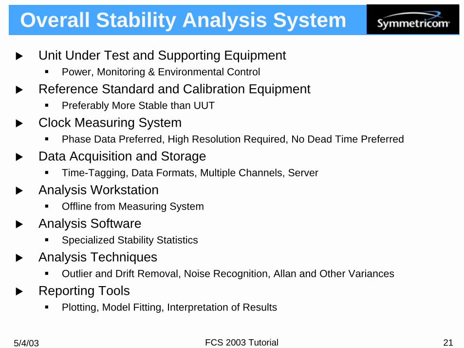
Overall Stability Analysis System! Unit Under Test and Supporting Equipment

! Power, Monitoring & Environmental Control

! Reference Standard and Calibration Equipment! Preferably More Stable than UUT

! Clock Measuring System! Phase Data Preferred, High Resolution Required, No Dead Time Preferred

! Data Acquisition and Storage! Time-Tagging, Data Formats, Multiple Channels, Server

! Analysis Workstation! Offline from Measuring System

! Analysis Software! Specialized Stability Statistics

! Analysis Techniques! Outlier and Drift Removal, Noise Recognition, Allan and Other Variances

! Reporting Tools! Plotting, Model Fitting, Interpretation of Results


Measurement Systems! A frequency counter can be used to directly make frequency

measurements with modest resolution! Higher resolution can be obtained from the following popular

measurement system configurations:

! Heterodyne System! Offset Reference! Narrowband! High Resolution! Frequency Only! Dead Time

! Time Interval Counter! Std Freq Reference

! Wide Freq Range! Fair Resolution! Phase Measured! No Dead Time! Simple


Measurement Systems (Con’t)! Dual Mixer Time Interval

! Offset Reference! Narrowband! High Resolution! Phase Measured! No Dead Time! Multiple Channels! Complex

! High resolution clock measuring systems are available commercially [ME-6], [ME-7], [ME-8]


Data Format! The essential data are an array of equally-spaced phase or frequency

values taken at particular measurement interval.! The data must have sufficient resolution to support the analysis. This

can require many orders of magnitude of dynamic range, particularly for frequency data taken with an ordinary frequency counter, or long-term phase data for a source having a large frequency offset.

! The data may have an associated time tag array, which can be a significant advantage for relating the data to other events. Use of the Modified Julian Date (MJD) is recommended.

! Data is most often stored as numeric ASCII characters, which provides the easiest transfer between different hardware and software.

! Non-numeric characters are often included as header information or comments, but are best put on separate lines.


Phase vs. Frequency Data! Phase data is preferred because it can be used to obtain frequency

data, but the reverse it not strictly true. Absolute phase cannot be reconstructed from frequency data, and a gap in the frequency data means that phase continuity is lost.

! Phase data can be used at a longer averaging time by simply re-sampling (decimating) it. Frequency data must be averaged to accomplish this, a process that takes much longer in a stabilityalgorithm. It is generally faster (sometimes much faster) to convert frequency data to phase data before performing a stability calculation.

! Phase data applies directly to timing applications, and is fundamental for time distribution systems.

! Frequency data is often easier to “read”. Outliers are more apparent, frequency changes are directly seen, and drift is more obvious.

! Frequency data is the more fundamental for most internal aspects of a frequency source.


Basic Analysis Sequence

→ →

Phase Data Convert to Freq Remove Outlier

0.000000000000000e+008.999873025741449e-071.799890526185009e-062.699869215098003e-063.599873851209537e-064.499887627663997e-065.399836191440859e-066.299833612216789e-067.199836723454638e-068.099785679257264e-068.999774896024524e-069.899732698242008e-06

Etc.

Phase data is just a ramp with slope corresponding to freq offset.

Outlier obvious in freq data – must remove it to continue analysis.

Can now see noise and drift.

Visual inspection of data is an important preprocessing step!


Basic Analysis Sequence (Con’t)

→ → →

↓

Remove Freq Offset Remove Freq Drift

Analyze Stability

Get Freq Residuals

Quadratic shape is due to freq drift -can now begin to see phase fluctuations.

Phase and freq residuals allow noise to be clearly seen.

Notice W & F FM Slopes at simulated levels


Preprocessing! Preprocessing is usually necessary before the formal stability analysis

is started.! Phase data may be decimated or frequency data averaged to a longer

tau. This will shorten the data file and make subsequent processing faster, but is a disadvantage for overlapping and total statistics.

! Phase <-> Frequency conversions may be performed.! The data may be plotted and examined visually for steps, jumps, spikes,

glitches, interference and other anomalies.! A portion of the data may be selected for analysis.! Outliers may be found and removed (with discretion). One should

understand why the data point is invalid.! Frequency offset may be removed.! Frequency drift may be analyzed and removed.


Phase-Frequency Conversions! Phase data can be converted to frequency data by dividing the 1st

difference of phase by tau: yi = (xi - xi-1) / τ.! Frequency data can be converted to phase data by multiplying the

frequency by tau and adding it to the phase: xi = xi-1 + (yi-1) · τ.! Phase to frequency conversion is straightforward unless the two phase

values are the same, which gives y = 0, and can be confused with a gap. Using a small non-zero value (e.g. 1e-99) will solve this. But two identical adjacent phase values can be a sign of data quantization or a measurement problem.

! Frequency to phase conversion is undefined if there is a gap in the data. To preserve phase continuity, the average frequency value can be used to integrate through the gap.

! The individual time tag interval can be used instead of a fixed tau for non uniformly-spaced data.


Outliers! It is important to have (and use) a consistent way to identify and remove

outliers, based on the the methods of robust statistics [R-2].! This is much easier to do for frequency (rather than phase) data.! An outlier is an extreme data point that is significantly larger or smaller

than most others (often a case of “I’ll know it when I see it”).! The median is a robust way to determine the center value (an outlier

affects the mean).! The deviation from the median is a robust way to determine whether a

point is an outlier.! The median absolute deviation (MAD) [R-3] is a robust way to set the

criterion for an outlier. It is the median of the (scaled) absolute deviations of the data points from their median value, and is defined as:

MAD = Median { | y(i) - m | / 0.6745 }

where m=Median { y(i) }, and the factor 0.6745 makes the MAD equal to the standard deviation for normally distributed data.

! An outlier criterion of 5X the MAD is usually a good choice.


Frequency Offset

1. Linear Fit: The first (optimal for white PM noise) uses a least-squares linear fit to the phase data, x(t) = a + bt, where slope = y(t) = b.

2. Endpoints: The second method simply uses the difference between the first and last points of the phase data, slope = y(t) = [ x(end) − x(start) ] / (M-1), where M = # phase data points. This method (optimal for white FM noise) can be used to match the two endpoints.

Frequency offset is usually calculated for frequency data as the average (mean) of the frequency values.

Frequency offset may be calculated for phase data by either of two methods:


Drift Analysis and Removal

1. Quadratic Fit: The first is a least-squares quadratic fit to the phase data, x(t) = a + bt + ct², where y(t) = x'(t) = b + 2ct, slope = y'(t) = 2c. This method is optimum for white PM noise [G-16].

2. 2nd Differences: The second method is the average of the 2nd

differences of the phase data, y(t) = [x(t+τ)−x(t)]/τ, slope = [y(t+τ)−y(t) ]/τ = [ x(t+2τ)−2x(t+τ)+x(t)]/τ².This method is optimum for random walk FM noise [D-4].

3. 3-Point: The third method uses the 3 points at the start, middle and endof the phase data, slope = 4[x(end)−2x(mid)+x(start)]/(Mτ)², where M = # data points It is the equivalent of the bisection method for frequency data [D-3].

Three methods are commonly used to analyze frequency drift in phase data:


Drift Analysis and Removal (Con’t)

1. Linear Fit: The first, the default, is a least squares linear regression tothe frequency data, y(t) = a+bt, where a = intercept, b = slope = y'(t). This is the optimum method for white FM noise.

2. Bisection: The second method computes the drift from the frequency averages over the first and last halves of the data, slope = 2 [ y(2nd half) − y(1st half) ] / (Nτ), where N = # points. This bisection method is optimum for white and random walk FM noise.

3. Log Fit: The third method, a log model of the form (see MIL-O-55310B), y(t) = a·ln(bt+1), where slope = y'(t) = ab/(bt+1) which applies to frequency stabilization.

4. Diffusion Fit: The last frequency drift method is a diffusion (√ t) model of the form y(t) = a+b(t+c)1/2, where slope=y'(t)=½·b(t+c)-1/2.

Four methods are commonly used to analyze frequency drift in frequency data:


Bias and Confidence! It is not enough to simply calculate one of these statistics. It is also

necessary to know what value it is expected to converge to, and how closely it has done so.

! The Allan variance is defined so that its expected value is the same as the standard variance for white FM noise. Most of the other clock statistics are either defined likewise, or are biased estimators of the Allan variance for which (noise and sample size dependent) corrections must be applied.

! Thus, properly applied and corrected, all of these statistics converge to the same expected value, with increasing confidence as the number of samples increases.

! The uncertainly in the result can be estimated and used to set confidence intervals and error bars, using the theory of Χ2 statistics that applies to variances.

! This requires knowledge of the equivalent number of degrees of freedom (EDF), which is also a function of the noise type and number of samples.


Noise Identification! Noise type identification is important not only for understanding the

physical basis of the instability but also to apply bias corrections and to set confidence limits.

! The noise type may be known a priori, or can be determined by a preliminary analysis from the slope of a log σ vs. log τ stability plot.

! Preferably, the noise identification is performed automatically at each averaging time during a stability run to support bias corrections and error bar determination.

! A way for automatic noise identification is to calculate additional vari-ances (e.g. standard or mod Allan) whose ratio to the desired variance (e.g. Allan) is dependent in a known way on the noise type [N-6].

! The Barnes B1 and R(n) ratios can be used for this purpose.! B1 is the ratio of the standard (N-sample) and Allan (2-sample)

variances [N-3].! R(n) is the ratio of the modified Allan and Allan variances [G-16].! Analytic expressions are available to relate these ratios to the noise

type and number of data samples.


Noise Identification (Con’t)The dominant power law noise type can be estimated by comparing the ratio of the N-sample (standard) variance to the 2-sample (Allan) variance of the data (the B1 bias factor) to the value expected of this ratio for the pure noise types (for the same averaging factor). This method of noise identification, while not perfect, is reasonably effective in most cases. The main limitations are (1) its inability to distinguish between white and flicker PM noise, and (2) its limited precision at large averaging factors where there are few analysis points. The former limitation can be overcome by supplementing the B1 ratio test with one based on R(n), the ratio of the modified Allan variance to the normal Allan variance. That technique is applied to members of the modified family of variances (MVAR, TVAR, and MTOT). The second limitation can be avoided by using the previous noise type estimate at the longest averaging time of an analysis run. One further limitation is that the R(n) ratio is not meaningful at a unity averaging factor. A description of this power law noise identification method can be found in Reference [N-6].


Confidence IntervalsSample variances are distributed according to the expression:

EDF · s²χ² =

σ²

where χ² is the Chi-square, s² is the sample variance, σ² is the true variance, and EDF is the Equivalent number of Degrees of Freedom (not necessarily an integer). The EDF is determined by the number of analysis points and the noise type. Single or double-sided confidence intervals (error bars) with a certain confidence factor may be set for variances based on χ² statistics. The general procedure is to choose a confidence factor, p, calculate the corresponding χ² value, determine the EDF from the variance type, noise type and number of analysis points, and then set the statistical limit(s) on the variance. For double-sided limits:

EDF EDFσ²min = s2 ⋅ and σ²max = s2 ⋅

χ²(p, EDF) χ²(1-p, EDF)


EDF! The Equivalent # of Χ2 Degrees of Freedom (EDF) is needed to

determine confidence intervals and set error bars for a varianceestimate.

! The EDF value depends on the variance type, the noise type, and the number of data points used in the analysis.

! Empirical formulae exist for determining the approximate EDF value.! Some variance types use a large number of highly-correlated 2nd

differences to obtain a larger EDF for better confidence.

Variance Type EDF Determination Method ReferenceAllan & Hadamard σ/√N & Kn, see p. TN-182 [G-16]Overlapping Allan See Table 12.4 (as corrected) [G-11]Modified & Time Allan HEDF w/ modified args [HV-8]Overlapping Hadamard HEDF [HV-8]Total See Table I [T-7]Modified & Time Total See §4.2 & Table 1 [MT-1]Hadamard Total See Eq. (7) & Table 1 [HV-9]Thêo1 Currently Under Investigation [TH-1]


ADEV EDF Example

1

10

100

1000

1 10 100

EDF=[(3(N-1)/2m)-(2(N-2)/N)]⋅[4m2/(4m2+5)]500

100

50

10

5

N=

Averaging Factor, m

EDF

ADEV EDF for W FM Noise

EDF falls offto 1at m≈N/2


ADEV EDF Example (Con’t)

1

10

100

1 10 100

α Noise 2 W PM 1 F PM 0 W FM-1 F FM-2 RW FM

-2

-1

0

1

2α=

Averaging Factor, m

EDFADEV EDF for N=100

EDF generally lower for more divergent noise types

EDF nearly independent of m for W PM noise

EDF ≈ N/m for α ≤ 0


EDF vs Variance Type

1

10

100

200

1 10 100

TotalHadamard TotalAllanModified TotalHadamardModified Allan

Averaging Factor, m

EDF

EDF for N=100 W FM Noise

EDF larger for total variances compared with their non-total equivalents


Postprocessing! Dead Time Correction

! Apply Barnes B2 and B3 Bias Ratio! Important for non-white noises and large dead time ratios

! Reference Correction! Separation of Variances

! 1 of 2 Clocks Correction! Divide sigma by √2! Use when measuring 2 identical units

! Noise Line Fitting! Fit power law noise lines to stability data

! Interpretation of Results! Data presentation and discussion! Correlation with clock physics! Understanding of environmental effects! Explanations for anomalies! Suitability for application


Dead Time

Dead time between frequency measurements can affect the results of a stability analysis, and should be avoided if possible.

Otherwise, the Barnes B2 and B3bias ratios should be used to correct for the effect of dead time [DT-2].

This is an example of the effect of dead time on W PM noise sampled with a 100-second measurement once per hour, and the use of dead time corrections.


Separation of Variances! The so-called “3-Cornered Hat” method can be used to separate the

variances of the unknown and reference clocks in a stability measurement [3C-2], [3C-10].

! Three measurements are made of the sources in pairs, and are processed to obtain the individual variances.

! The method works best with large data sets for uncorrelated devices having similar stabilities – otherwise non-physical negative variances can result. A “perfect” reference is still the best!

Measured ADEVs Separated ADEVs


Phase Steps/Frequency SpikesThe Allan deviation of a frequency record having large spike (a phase step) has a τ-1/2 characteristic [G-13]. This can be a source of confusion, but can also be used as a means for simulation. For example, adding a single large central outlier (e.g. 106) to an otherwise much smaller 1000-point data set yields a white FM noise level of σy(τ0)=[(106)2/(1000-1)]1/2 = 3.16386e4.


Data QuantizationWhile it is desirable to have sufficient resolution that the data is noise rather than resolution limited, highly quantized data can provide good stability information provided that there is a least 1 bit of meaningful variation.

Random telegraph signal representing frequency data having a white FM noise characteristic


Cyclic Environmental SensitivityThe combination of an environmental sensitivity and a cyclic disturbance will cause the time-domain stability to display a distinctive pattern ofmaxima and minima at the half period and period of the stimulus as given by the expression:

where: ∆f/f = peak frequency deviation, T = period of disturbance, and τ = averaging time.

An example of such a stability record is shown below. This is a simulation of the stability of a GPS Block IIR rubidium atomic frequency standard (RAFS) with typical white FM and flicker FM noise levels of 2x10-12τ-1/2 and 2x10-14 respectively, plus a temperature coefficient of 2x10-13/°C, when exposed to a sinusoidal orbital temperature variation of 5°C p-p with a 12-hour period. The actual clock has a baseplate temperature controller (BTC) that reduces this thermal sensitivity to below the noise level. Even this large periodic variation does not prevent determining the underlying noise level.


Cyclic Environmental Sensitivity


Vibrational Modulation

The same general expression applies to the effect of vibrational modulation on the stability of a frequency source. It should be noted that the envelope of the resulting stability plot shows both (at the top) the vibrational FM (1x10-9·√2 rms at 1/2·fvib) and the noise (1x10-12τ-1). Minima occur at averaging times equal to multiples of the vibration period.


HistogramA histogram shows the amplitude distribution of the phase or frequency fluctuations, and can provide insight regarding them. One can expect a normal (Gaussian) distribution for a reasonably-sized data set, and a different (e.g. bimodal) distribution can be a sign of a problem. For a normal distribution, the standard deviation is approximately equal to the half-width at half-height (HWHA=1.177σ) .


Power Spectral DensitiesFrequency stability is described in the frequency domain by several power spectral densities:

PSD of Frequency Fluctuations Sy(f)The power spectral density (PSD) of the fractional frequency fluctuations y(t) in units of 1/Hz is given by Sy(f) = h(α)·fα, where f=sideband frequency, Hz and h(α) is an intensity coefficient.

PSD of Phase Fluctuations Sφ(f)The PSD of the phase fluctuations in units of rad²/Hz is given by Sφ(f) = (2πν0)² · Sx(f), where ν0=carrier frequency, Hz.

PSD of Time Fluctuations Sx(f)The PSD of the time fluctuations x(t) in units of sec²/Hz is given by Sx(f) = h(β)·fβ = Sy(f)/(2πf)², where β=α-2. The time fluctuations are related to the phase fluctuations by x(t)= φ(t)/2πν0.

SSB Phase Noise £(f)The SSB phase noise in units of dBc/Hz is given by £(f) = 10·log[½ · Sφ(f)]. This is the most common engineering unit to specify phase noise.


Domain ConversionsConversions can be made between time and frequency domain stability measures. These conversions are unique from the frequency domain, but may not be for the opposite case. For the Allan variance, the relationship is:

And, for the modified Allan and time deviations, the relationship is:

These conversions may be performed by numerical integration.


Domain Conversions (Con’t)Domain conversions may be made for power law noise models by using the following conversion formulae:

Noise Type σ²y(τ) Sy(f) RW FM A·f2 ·Sy(f)·τ1 A-1·τ-1·σ²y(τ)·f-2F FM B·f1 ·Sy(f)·τ0 B-1·τ0·σ²y(τ)·f-1W FM C·f0 ·Sy(f)·τ-1 C-1·τ1·σ²y(τ)·f0F PM D·f-1·Sy(f)·τ-2 D-1·τ2·σ²y(τ)·f1W PM E·f-2·Sy(f)·τ-2 E-1·τ2·σ²y(τ)·f2

where:A=4π²/6B=2·ln2C=1/2D=1.038+3·ln(2πfhτ0)/4π²E=3fh/4π²

and fh is the upper cutoff frequency of the measuring system in Hz, and τ0is the basic measurement time. The fh factor applies only to white and flicker PM noise.


Spectral Analysis

Spectral analysis is another method to characterize frequency stability. In the context of the time-domain techniques considered here, it can provide additional information about the noise type, and show the presence of interference.

The subject of spectral analysis is a broad one. Issues include reducing bias with windowing (tapering) functions, and reducing variance with averaging (smoothing). A distinguishing aspect of its application to frequency stability analysis is the emphasis on noise, rather than discrete components. Besides FFT-based periodograms, the multitaper method is recommended.


Spectral Analysis (Con’t)

Commercial instruments are available [ME-6] to take relatively fast, high resolution time domain phase data and present it both as Allan deviation and £(f), as shown below for a small rubidium frequency standard.


ReportingThe results of a stability analysis are usually presented as a combination of textual, tabular and graphic forms. The text describes the device under test, the test setup, and the methodology of the data preprocessing and analysis, and summarizes the results. The latter often includes a table of the stability statistics. Graphical presentation of the data at each stage of the analysis is generally the most important aspect of presenting the results. For example, these are often a series of plots showing the phase and frequency data with an aging fit, phase and frequency residuals with the aging removed, and stability plots with noise fits and error bars. Plot titles, sub-titles, annotations and inserts can be used to clarify and emphasize the data presentation. The results of several stability runs can be combined, possibly along with specification limits, into a single composite plot. The various elements can be combined into a single electronic document for easy printing and transmittal.


Data PlotsData plotting is often the most important step in the analysis of frequency stability. Visual inspection can provide vital insight into the results, and is an important "preprocessor'' before numerical analysis. A plot also shows much about the validity of a curve fit.

Phase data is generally plotted as line segments connecting the data points. This presentation properly conveys the integral nature of the phase data.

Frequency data is often plotted the same way, simply because that is the way plotting is usually done. But a better presentation is a flat horizontal line between the frequency data points. This shows the averaging time associated with the frequency measurement, and mimics the analog chart record from a counter.

As the density of the data points increases, there is essentially no visual difference between the two plotting methods, and the point method is faster.


Data Plots (Con’t)001 002 003 004 005

006 007 008 009 010

011 012 013 014 015

016 017 018 019 020

Small multiple plots can be a useful visual tool for comparing behavior, as shown in these aging plots for GPS Rb clocks [SW-7].

Fits to linear, log, diffusion or other drift models can support stability analysis and aid in understanding the physical processes involved.


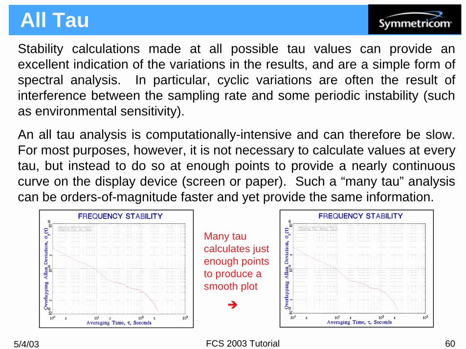
Stability Plots

Stability plots generally take the form of graphs of log versus log , often with error bars to shown the precision of the results. The slope of the σy(τ) characteristic depends on the type of noise. It is customary to show points at binary increments of tau. These are equally spaced on the log scale, and are the result of successive averaging by two. Such a run usually ends when there are too few analysis points (say < 7) for reasonable confidence. A run for all possible values, while slow, can provide valuable information since it is, in effect, a form of spectral analysis that can show periodic instabilities such as environmental effects. Such an all-tau run can be made much faster by spacing the points no closer than can be seen on the display device.


All TauStability calculations made at all possible tau values can provide an excellent indication of the variations in the results, and are a simple form of spectral analysis. In particular, cyclic variations are often the result of interference between the sampling rate and some periodic instability (such as environmental sensitivity).

An all tau analysis is computationally-intensive and can therefore be slow. For most purposes, however, it is not necessary to calculate values at every tau, but instead to do so at enough points to provide a nearly continuous curve on the display device (screen or paper). Such a “many tau” analysis can be orders-of-magnitude faster and yet provide the same information.

Many tau calculates just enough points to produce a smooth plot

!


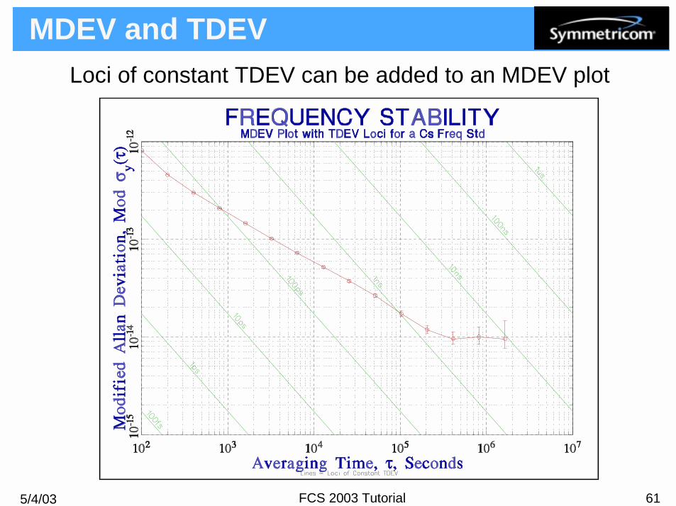
MDEV and TDEVLoci of constant TDEV can be added to an MDEV plot


Software Validation

1. Manual Analysis: The results obtained by manual analysis of small data sets (such as NBS Monograph 140 Annex 8.E [G-4]) can be compared with the new program output. This is always good to do to get a "feel'' for the process.

2. Published Results: The results of a published analysis or test suite can be compared with the new program output [SW-3], [SW-4].

3. Other Programs: The results obtained from other specialized stability analysis programs [SW-6], or from a previous generation computer or operating system, can be compared with the new program output.

4. General Programs: The results obtained from industry standard, general purpose mathematical and spreadsheet programs (such as MathCAD and Excel) can be compared with the new program output.

Several methods are available to validate frequency stability analysis software:


Software Validation (Con’t)

5. Consistency Checks: The new program should be verified for internal consistency, such as producing the same stability results from phase and frequency data. The standard and Allan variances should be approximately equal for white FM noise. The Allan and modified Allan variances, and total variance, should be identical for an averaging factor of 1. For other averaging factors, the modified Allan variance should be approximately one-half the normal Allan variance for white FM noise and τ >> τ0. The normal and overlapping Allan variances, and total variance, should be approximately equal, while the overlapping method and total variance provide better confidence of the stability estimates. The various methods of drift removal should yield similar results.

6. Simulated Data: Simulated clock data can also serve as a useful cross check. Known values of frequency offset and drift can be inserted, analyzed and removed. Known values of power law noise can be generated, analyzed, plotted and modeled.


References - General1. Special Issue on Frequency Stability, Proc. IEEE, Vol. 54, Feb. 1966. 2. Proc. IEEE, Vol. 55, June 1967. 3. J.A. Barnes, et. al., “Characterization of Frequency Stability”, IEEE Trans.

Instrum. Meas., Vol. IM-20, No. 2, pp. 105-120, May 1971. 4. B.E. Blair (Editor), "Time and Frequency: Theory and Fundamentals", NBS

Monograph 140, U.S. Department of Commerce, National Bureau of Standards, May 1974.

5. G. Winkler, "A Brief Review of Frequency Stability Measures", Proc. 8th PTTI Meeting, pp. 489-527, Dec. 1976.

6. J. Rutman, "Oscillator Specifications: A Review of Classical and New Ideas", Proc. 31th Annu. Symp. on Freq. Contrl., pp.291-310, June 1977.

7. J. Vanier and M. Tetu, "Time Domain Measurement of Frequency Stability", Proc. 10th PTTI Meeting, pp. 247-291, Nov. 1978.

8. P.Lesage and C. Audoin, “Characterization and Measurement of Time and Frequency Stability”, Radio Science, Vol. 14, No. 4, pp. 521-539, 1979.

G-#

http://www.ieee-uffc.org/archive/fc/proceed/1977/proceed/s7710291.pdf

http://home.attbi.com/~lizriley/JVTutorial.pdf


References - General (Con’t)9. D.A. Howe, D.W. Allan and J.A. Barnes, "Properties of Signal Sources and

Measurement Methods'', Proc. 35th Annu. Symp. on Freq. Contrl., pp. 1-47, May 1981. Also available on line at NIST web site.

10. V.F. Kroupa (Editor), Frequency Stability: Fundamentals and Measurement, IEEE Press, Institute of Electrical and Electronic Engineers, New York, 1983, ISBN 0-87942-171-1.

11. S.R. Stein, "Frequency and Time - Their Measurement and Characterization'', Chapter 12, pp.191-416, Precision Frequency Control, Vol. 2, Edited by E.A. Gerber and A. Ballato, Academic Press, New York, 1985, ISBN 0-12-280602-6.

12. Proc. IEEE, Vol. 74, Jan. 1986. 13. C.A. Greenhall, "Frequency Stability Review", Telecommunications and Data

Acquisition Progress Report 42-88, Oct-Dec 1986, Jet Propulsion Laboratory, Pasadena, CA, pp. 200-212, Feb. 1987.

14. D.W. Allan, “Time and Frequency (Time-Domain) Characterization, Estimation, and Prediction of Precision Clocks and Oscillators”, IEEE Trans. Ultrasonics, Ferroelectrics and Freq. Contrl., Vol. UFFC-34, No. 6, pp. 647-654, Nov. 1987.

G-#



http://www.bldrdoc.gov/timefreq/phase/Properties/main.htm

http://www.amazon.com/exec/obidos/ISBN%3D0122806026/104-9196908-8979922

http://tmo.jpl.nasa.gov/tmo/progress_report/42-88/88Z.PDF

http://www.ieee-uffc.org/archive/uffc/trans/trans/1987/t8760647.pdf

http://www.ieee-uffc.org/archive/uffc/trans/trans/1987/t8760647.pdf


References - General (Con’t)15. D.W. Allan, et al., "Standard Terminology for Fundamental Frequency and Time

Metrology", Proc. 42nd Annu. Freq. Control Symp., pp. 419-425, June, 1988. 16. D.B Sullivan, D.W Allan, D.A. Howe and F.L.Walls (Editors), "Characterization

of Clocks and Oscillators", NIST Technical Note 1337, U.S. Department of Commerce, National Institute of Standards and Technology, March 1990.

17. D.W. Allan, “Characterization of Precision Clocks and Oscillators”, Class Notes, NRL Workshop, Nov. 1990.

18. D.W. Allan, "Time and Frequency Metrology: Current Status and Future Considerations'', Proc. 5th European Freq. and Time Forum, pp. 1-9, March 1991.

19. Special Issue on Time and Frequency, Proc. IEEE, Vol. 79, July 1991. 20. J. Rutman and F. L. Walls, "Characterization of Frequency Stability in Precision

Frequency Sources", Proc. IEEE, Vol. 79, July 1991. 21. J.A. Barnes, "The Analysis of Frequency and Time Data", Austron, Inc., Dec.

1991.22. W.J. Riley, "The Calculation of Time Domain Frequency Stability”, Hamilton

Technical Services, 2002.23. W.J. Riley, "The Basics of Frequency Stability Analysis", Hamilton Technical

Services, 2000.

G-#



http://www.boulder.nist.gov/timefreq/general/tn1337/


http://www.ieee-uffc.org/archive/uffc/special/misc/e917/e9170952.pdf

http://www.ieee-uffc.org/archive/uffc/special/misc/e917/e9170952.pdf

http://www.wriley.com/paper1ht.htm



References - Standards1. "Characterization of Frequency and Phase Noise", Report 580, International

Radio Consultative Committee (C.C.I.R.), pp. 142-150, 1986. 2. MIL-PRF-55310, Oscillators, Crystal, General Specification For. 3. R.L. Sydnor (Editor), “The Selection and Use of Precise Frequency Systems”,

ITU-R Handbook, 1995.4. Guide to the Expression of Uncertainty in Measurement, International

Standards Organization, 1995, ISBN 92-67-10188-9. 5. "IEEE Standard Definitions of Physical Quantities for Fundamental Frequency

and Time Metrology - Random Instabilities", IEEE Std 1139-1999, July 1999. 6. Proc. IEEE-NASA Symp. on the Definition and Measurement of Short-Term

Frequency Stability, NASA SP-80, Nov. 1964.

ST-#

http://www.dscc.dla.mil/Programs/MilSpec/ListDocs.asp?BasicDoc=MIL-PRF-55310


References - Allan Variance1. D.W. Allan, "Allan Variance", Allan's TIME. 2. D.W. Allan, "The Statistics of Atomic Frequency Standards'', Proc. IEEE, Vol.

54, No. 2, pp. 221-230, Feb. 1966. 3. "Characterization of Frequency Stability", NBS Technical Note 394, U.S

Department of Commerce, National Bureau of Standards, Oct. 1970.4. J.A. Barnes, et al, "Characterization of Frequency Stability", IEEE Trans.

Instrum. Meas., Vol. IM-20, No. 2, pp. 105-120, May 1971. 5. J.A. Barnes, “Variances Based on Data with Dead Time Between the

Measurements”, NIST Technical Note 1318, U.S. Department of Commerce, National Institute of Standards and Technology, 1990.

6. C.A. Greenhall, "Does Allan Variance Determine the Spectrum?", Proc. 1997 Intl. Freq. Cont. Symp., pp. 358-365, June 1997.

7. C.A. Greenhall, “Spectral Ambiguity of Allan Variance”, IEEE Trans. Instrum. Meas., Vol. IM-47, No. 3, pp. 623-627, June 1998.

AV-#

http://www.allanstime.com/AllanVariance/index.html

http://horology.jpl.nasa.gov/papers/spectrum.pdf

http://horology.jpl.nasa.gov/papers/specambi.pdf


Refs - Mod Allan Variance1. D.W. Allan and J.A. Barnes, "A Modified Allan Variance with Increased

Oscillator Characterization Ability", Proc. 35th Annu. Symp. on Freq. Contrl., pp. 470-474, May 1981.

2. P. Lesage and T. Ayi, “Characterization of Frequency Stability: Analysis of the Modified Allan Variance and Properties of Its Estimate”, IEEE Trans. Instrum. Meas., Vol. IM-33, No. 4, pp. 332-336, Dec. 1984.

3. C.A. Greenhall, "Estimating the Modified Allan Variance", Proc. 1995 IEEE Freq. Contrl. Symp., pp. 346-353, May 1995.

4. C.A. Greenhall, "The Third-Difference Approach to Modified Allan Variance", IEEE Trans. Instrum. Meas., Vol. IM-46, No. 3, pp. 696-703, June 1997.

MV-#




http://horology.jpl.nasa.gov/papers/thirddiff.pdf


References - Time Variance1. D.W. Allan and H. Hellwig, “Time Deviation and Time Prediction Error for Clock

Specification, Characterization, and Application”, March 1981. 2. D.W. Allan, D.D. Davis, J. Levine, M.A. Weiss, N. Hironaka, and D. Okayama,

"New Inexpensive Frequency Calibration Service From NIST'', Proc. 44th Annu.Symp. on Freq. Contrl., pp. 107-116, June 1990.

3. D.W. Allan, M.A. Weiss and J.L. Jespersen, "A Frequency-Domain View of Time-Domain Characterization of Clocks and Time and Frequency Distribution Systems'', Proc. 45th Annu. Symp. on Freq. Contrl., pp. 667-678, May 1991.

TV-#






Refs - Hadamard Variance1. Jacques Saloman Hadamard (1865-1963), French mathematician.2. R.A. Baugh, "Frequency Modulation Analysis with the Hadamard Variance",

Proc. 25th Annu. Symp. on Freq. Contrl., pp. 222-225, April 1971. 3. B. Picinbono, "Processus a Accroissements Stationnaires", Ann. des telecom,

Tome 30, No. 7-8, pp. 211-212, July-Aug, 1975. 4. K. Wan, E. Visr and J. Roberts, "Extended Variances and Autoregressive

Moving Average Algorithm for the Measurement and Synthesis of Oscillator Phase Noise", 43rd Annu. Symp. on Freq. Contrl., pp.331-335, June 1989.

5. S.T. Hutsell, "Relating the Hadamard Variance to MCS Kalman Filter Clock Estimation", Proc. 27th PTTI Meeting, pp. 291-302, Dec. 1995.

6. S.T. Hutsell, "Operational Use of the Hadamard Variance in GPS", Proc. 28th PTTI Meeting, pp. 201-213, Dec. 1996.

7. D.N. Matsakis and F.J. Josties, "Pulsar-Appropriate Clock Statistics", Proc. 28th PTTI Meeting, pp. 225-236, Dec. 1996.

8. C.A. Greenhall, private communication, May 1999 and March 2000. The edf for the overlapping Hadamard variance can be found by an algorithm developed by C.A. Greenhall based on its generalized autocovariance function.

9. D. Howe, et al., “A Total Estimator of the Hadamard Function Used For GPS Operations”, Proc. 32nd PTTI Meeting, pp. 255-268, Nov. 2000.

10. W.J. Riley, “The Hadamard Variance”, Hamilton Technical Services, 1999.

HV-#

http://www-groups.dcs.st-and.ac.uk/~history/Mathematicians/Hadamard.html





http://www.wriley.com/TotHvar-PTTI-00.pdf

http://www.wriley.com/TotHvar-PTTI-00.pdf



References - Total Variance1. D.A. Howe, "An Extension of the Allan Variance with Increased Confidence at

Long Term," Proc. 1995 IEEE Int. Freq. Cont. Symp., pp. 321-329, June 1995. 2. D.A. Howe and K.J. Lainson, "Simulation Study Using a New Type of Sample

Variance," Proc. 1995 PTTI Meeting, pp. 279-290, Dec. 1995. 3. D.A. Howe and K.J. Lainson, "Effect of Drift on TOTALDEV", Proc. 1996 Intl.

Freq. Cont. Symp. , pp. 883-889, June 1996 4. D.A. Howe, "Methods of Improving the Estimation of Long-term Frequency

Variance," Proc. 1997 European Frequency and Time Forum, pp. 91-99, March 1997.

5. D.A. Howe & C.A. Greenhall, "Total Variance: A Progress Report on a New Frequency Stability Characterization", pp. 39-48, Proc. 1997 PTTI Meeting, Dec. 1997.

6. D.B. Percival and D.A. Howe, "Total Variance as an Exact Analysis of the Sample Variance", Proc. 1997 PTTI Meeting, Dec. 1997.

7. C.A. Greenhall, D.A. Howe and D.B Percival, “Total Variance, an Estimator of Long-Term Frequency Stability”, IEEE Trans. Ultrasonics, Ferroelectrics and Freq. Contrl., Vol. UFFC-46, No. 5, pp. 1183-1191, Sept. 1999.

T-#




http://horology.jpl.nasa.gov/papers/totvar_ptti.pdf

http://horology.jpl.nasa.gov/papers/totvar_ptti.pdf

http://horology.jpl.nasa.gov/papers/totvar_uffc99.pdf

http://horology.jpl.nasa.gov/papers/totvar_uffc99.pdf


Refs - Total Variance (Con’t)8. D.A. Howe, “The Total Deviation Approach to Long-Term Characterization of

Frequency Stability”, IEEE Trans. Ultrasonics, Ferroelectrics and Freq. Contrl., Vol. UFFC-47, No. 5, pp. 1102-1110, Sept. 2000.

9. D.A. Howe, "Total Variance Explained", Proc. 1999 Joint Meeting of the European Freq. and Time Forum and the IEEE Freq. Contrl. Symp., pp. 1093-1099, April 1999.

10. D.A. Howe and T.K. Peppler, "Definitions of Total Estimators of Common Time-Domain Variances", Proc. 2001 Intl. Freq. Cont. Symp. , pp. 127-132, June 2001

T-#

http://www.ieee-uffc.org/archive/uffc/trans/toc/papers/00/sep1102.pdf

http://www.ieee-uffc.org/archive/uffc/trans/toc/papers/00/sep1102.pdf


http://www.boulder.nist.gov/timefreq/general/pdf/1481.pdf

http://www.boulder.nist.gov/timefreq/general/pdf/1481.pdf


Refs - Mod Total Variance1. D.A. Howe and F. Vernotte, "Generalization of the Total Variance Approach to

the Modified Allan Variance", Proc. 31th PTTI Meeting, pp.267-276, Dec. 1999.

MT-#

http://tycho.usno.navy.mil/ptti/ptti99/PTTI_1999_267.PDF

http://tycho.usno.navy.mil/ptti/ptti99/PTTI_1999_267.PDF


Refs - Time Total Variance1. M.A. Weiss and D.A. Howe, “Total TDEV”, Proc. 1998 IEEE Int. Freq. Cont.

Symp., pp. 192-198, June 1998.

TT-#



Thêo1 Variance1. D.A. Howe and T.K. Peppler, "Estimation of Very Long-Term

Frequency Stability Using a Special-Purpose Statistic", Proceedings of the 2003 IEEE International Frequency Control Symposium , May 2003 (to be published).

TH-#


References - MTIE1. P. Travella and D. Meo, “The Range Covered by a Clock Error in the Case of

White FM”, Proc. 30th Annu. PTTI Meeting, pp. 49-60, Dec. 1998. 2. P. Travella, A. Dodone and S. Leschiutta, “The Range Covered by a Random

Process and the New Definition of MTIE”, Proc. 28th Annu. PTTI Meeting, pp. 119-123, Dec. 1996.

3. Bregni, " Clock Stability Characterization and Measurement in Telecommunications”, IEEE Trans. Instrum. Meas., Vol. IM-46, No. 6, pp. 1284-1294, Dec. 1997.

4. Bregni, " Measurement of Maximum Time Interval Error for Telecommunications Clock Stability Characterization”, IEEE Trans. Instrum. Meas., Vol. IM-45, No. 5, pp. 900-906, Oct. 1996.

5. G. Zampetti, “Synopsis of Timing Measurement Techniques Used inTelecommunucations”, Proc. 24th PTTI Meeting, pp. 313-326, Dec. 1992.

6. M.J. Ivens, "Simulating the Wander Accumulation in a SDH SynchronisationNetwork", Master's Thesis, University College, London, UK, November 1997.

7. S. Bregni and S. Maccabruni, "Fast Computation of Maximum Time Interval Error by Binary Decomposition", IEEE Trans. I&M, Vol. 49, No. 6, Dec. 2000, pp. 1240-1244.

M-#

http://www.elet.polimi.it/Users/DEI/Sections/Telecom/Stefano.Bregni/PAPERS/clockstab.pdf

http://www.elet.polimi.it/Users/DEI/Sections/Telecom/Stefano.Bregni/PAPERS/clockstab.pdf

http://www.elet.polimi.it/Users/DEI/Sections/Telecom/Stefano.Bregni/PAPERS/mtiemeas.pdf

http://www.elet.polimi.it/Users/DEI/Sections/Telecom/Stefano.Bregni/PAPERS/mtiemeas.pdf

http://www.micronet.co.uk/thesis2.html

http://www.micronet.co.uk/thesis2.html


References - Multi-Variance1. F. Vernotte, E. Lantz, "Time Stability: An Improvement of the Multi-Variance

Method for the Oscillator Noise Analysis", Proc. 6th European Frequency and Time Forum, pp. 343-347, March 1992.

2. F. Vernotte, E. Lantz, J. Groslambert and J.J. Gagnepain, "A New Multi-Variance Method for the Oscillator Noise Analysis", Proc. 46th Annu. Symp. on Freq. Contrl., pp. 284-289, May 1992.

3. F. Vernotte, E. Lantz, J. Groslambert and J.J. Gagnepain, "Oscillator Noise Analysis: Multivariance Measurement", IEEE Trans. Instrum. Meas., Vol. IM-42, No. 2, pp. 342-350, April 1993.

4. F. Vernotte, E. Lantz, F. Meyer and F. Naraghi, "Simultaneneous Measurement of Drifts and Noise Coefficients of Oscillators: Application to the Analysis of the Time Stability of the Millisecond Pulsars" Proc. 1997 European Frequency and Time Forum, pp. 91-99, March 1997.

5. T. Walter, "A Multi-Variance Analysis in the Time Domain", Proc. 24th PTTI Meeting, pp. 413-424, Dec. 1992.

MU-#


Refs - Confidence Intervals1. J.A. Barnes and D.W. Allan, Variances Based on Data with Dead Time Between

the Measurements", NIST Technical Note 1318, U.S. Department of Commerce, National Institute of Standards and Technology, 1990.

2. C.A. Greenhall, "Recipes for Degrees of Freedom of Frequency Stability Estimators'', IEEE Trans. Instrum. Meas., Vol. 40, No. 6, pp. 994-999, Dec. 1991.

3. M.A. Weiss and C. Hackman, "Confidence on the Three-Point Estimator of Frequency Drift'', Proc. 24th Annu. PTTI Meeting, pp. 451-460, Dec. 1992.

4. M.A.Weiss and C.A. Greenhall, "A Simple Algorithm for Approximating Confidence on the Modified Allan Variance and the Time Variance", Proc. 28th Annu. PTTI Meeting, pp. 215-224, Dec. 1996.

5. D.A. Howe, "Methods of Improving the Estimation of Long-Term Frequency Variance", Proc. 11th European Freq. and Time Forum, pp. 91-99, March 1997.

6. F. Vernotte and M. Vincent, "Estimation of the Uncertainty of a Mean Frequency Measurement“, Proc. 11th European Freq. and Time Forum, pp. 553-556, March 1997.

7. P. Lesage and C. Audoin, "Estimation of the Two-Sample Variance with a Limited Number of Data", pp. 311-318.

CI-#

http://horology.jpl.nasa.gov/papers/avaredf_im.pdf

http://horology.jpl.nasa.gov/papers/avaredf_im.pdf


Refs – Conf Intervals (Con’t)8. P. Lesage and C. Audoin, "Characterization of Frequency Stability: Uncertainty

due to the Finite Number of Measurements", IEEE Trans. Instrum. Meas., Vol. 22, No. 2, pp.157-161, June 1973.

9. K. Yoshimura, "Degrees of Freedom of the Estimate of the Two-Sample Variance in the Continuous Sampling Method", IEEE Trans. Instrum. Meas., Vol. 38, No. 6, pp. 1044-1049, Dec. 1989.

10. W.J. Riley, “Confidence Intervals and Bias Corrections for the Stable32 Variance Functions”, Hamilton Technical Services, 2000.

CI-#

http://www.wriley.com/CI.htm

http://www.wriley.com/CI.htm


References - Drift1. C.A. Greenhall, "Removal of Drift from Frequency Stability Measurements", ",

Telecommunications and Data Acquisition Progress Report 42-65, July-Aug 1981, Jet Propulsion Laboratory, Pasadena, CA, pp. 127-132, 1981.

2. J.A. Barnes, "The Measurement of Linear Frequency Drift in Oscillators'', Proc. 15th Annu. PTTI Meeting, pp. 551-582, Dec. 1983.

3. M.A. Weiss and C. Hackman, "Confidence on the Three-Point Estimator of Frequency Drift", Proc. 24th Annu. PTTI Meeting, pp. 451-460, Dec. 1992.

4. M.A. Weiss, D.W. Allan and D.A. Howe, "Confidence on the Second Difference Estimation of Frequency Drift'', Proc. 1992 IEEE Freq. Contrl. Symp., pp. 300-305, June 1992.

5. “Long Term Quartz Oscillator Aging - A New Approach”, The Standard, Hewlett-Packard Co., pp. 4-5, Jan. 1994.

6. G.Wei, “Estimations of Frequency and its Drift Rate”, IEEE Trans. Instrum. Meas., Vol. 46, No. 1, pp. 79-82, Feb. 1997.

7. C.A. Greenhall, "A Frequency-Drift Estimator and Its Removal from Modified Allan Variance", Proc. 1997 IEEE Freq. Contrl. Symp., pp. 428-432, June 1997.

8. F. Vernotte and M. Vincent, “Estimation of the Measurement Uncertainty of Drift Coefficients Versus the Noise Levels", Proc. 12th European Freq. and Time Forum, pp. 222-227, March 1998.

D-#

http://tmo.jpl.nasa.gov/tmo/progress_report/42-65/65S.PDF






Refs - Noise Identification1. J.A. Barnes, "The Generation and Recognition of Flicker Noise", NBS Report

9284, U.S Department of Commerce, National Bureau of Standards, June 1967. 2. J.A. Barnes, “Effective Stationarity and Power Law Spectral Densities”, NBS

Frequency-Time Seminar Preprint, Feb. 1968. 3. J.A. Barnes, “Tables of Bias Functions, B1 and B2, for Variances Based on

Finite Samples of Processes with Power Law Spectral Densities”, NBS Technical Note 375, Jan. 1969.

4. J.A. Barnes and D.W. Allan, “Recognition and Classification of LF Divergent Noise Processes”, NBS Division 253 Class Notes, circa 1970.

5. J.A. Barnes, "Models for the Interpretation of Frequency Stability Measurements", NBS Technical Note 683, U.S Department of Commerce, National Bureau of Standards, Aug. 1976.

6. D. Howe, R. Beard, C. Greenhall, F. Vernotte and W. Riley, "A Total Estimator of the Hadamard Function Used for GPS Operations", Proceedings of the 32nd Annual Precise Time and Time Interval (PTTI) Systems and Applications Meeting, pp. 255-268, November 2000.

N-#


References - Dead Time1. J.A. Barnes and D.W. Allan, Variances Based on Data with Dead Time Between the

Measurements", NIST Technical Note 1318, U.S. Department of Commerce, National Institute of Standards and Technology, 1990.

2. D.B Sullivan, D.W Allan, D.A. Howe and F.L.Walls (Editors), "Characterization of Clocks and Oscillators", NIST Technical Note 1337, U.S. Department of Commerce, National Institute of Standards and Technology, TN-296-335, March 1990.

3. J.A. Barnes, "The Analysis of Frequency and Time Data", Austron, Inc., Dec. 1991.4. W.J. Riley, "Gaps, Outliers, Dead Time, and Uneven Spacing in Frequency Stability

Data”, Hamilton Technical Services, 2003.

DT-#



http://www.wriley.com/Gaps.htm

http://www.wriley.com/Gaps.htm


References - Simulation1. C.A. Greenhall and J.A. Barnes, "Large Sample Simulation of Flicker Noise",

Proc. 19th Annu. PTTI Meeting, pp. 203-217, Dec. 1987 and Proc. 24th Annu. PTTI Meeting, p. 461, Dec. 1992.

2. N.J. Kasdin and T. Walter, "Discrete Simulation of Power Law Noise", Proc. 1992 IEEE Freq. Contrl. Symp., pp. 274-283, May 1992.

3. T. Walter, “Characterizing Frequency Stability: A Continuous Power-Law Model with Discrete Sampling”, IEEE Trans. Instrum. Meas., Vol. 43, No. 1, pp. 69-79, Feb. 1994.

4. S.K. Park and K.W. Miller, "Random Number Generators: Good Ones are Hard to Find'', Comm. ACM, Vol. 31, No. 10, pp. 1192-1201.

S-#



Refs - Domain Conversions1. A.R. Chi, “The Mechanics of Translation of Frequency Stability Measures

Between Frequency and Time Domain Measurements”, Proc. 9th Annu. PTTI Meeting, pp. 523-548, Dec.1977.

2. J. Rutman, "Relations Between Spectral Purity and Frequency Stability”, pp. 160-165.

3. R. Burgoon and M.C. Fisher, “Conversion Between Time and Frequency Domain of Intersection Points of Slopes of Various Noise Processes”, 32th Annu. Symp. on Freq. Contrl., pp.514-519, June 1978.

4. W.F. Egan, “An Efficient Algorithm to Compute Allan Variance from Spectral Density”, IEEE Trans. Instrum. Meas., Vol. 37, No. 2, pp. 240-244, June 1988.

5. F. Vernotte, J. Groslambert and J.J. Gagnepain, “Practical Calculation Methods of Spectral Density of Instantaneous Normalized Frequency Deviation from Instantaneous Time Error Samples”, Proc. 5th European Freq. and Time Forum, pp. 449-455, March 1991.

DC-#




Refs - Robust Statistics1. D.B. Percival, "Use of Robust Statistical Techniques in Time Scale Formation",

Preliminary Report, U.S. Naval Observatory Contract No. N70092-82-M-0579, 1982.

2. Gernot M.R. Winkler, "Introduction to Robust Statistics and Data Filtering", Tutorial at 1993 IEEE Freq. Contrl. Symp., Sessions 3D and 4D, June 1, 1993.

3. V. Barnett and T. Lewis, Outliers in Statistical Data, 3rd Edition, John Wiley & Sons, Chichester, 1994, ISBN 0-471-93094-6.

R-#

http://www.wriley.com/ROBSTAT.htm


References - 3-Cornered Hat1. The term "3-cornered hat" was coined by J.E. Gray of NIST.2. J.E. Gray and D.W. Allan, "A Method for Estimating the Frequency Stability of

an Individual Oscillator", Proceedings of the 28th Annual Symposium on Frequency Control , May 1974, pp. 243-246.

3. S.R. Stein, "Frequency and Time - Their Measurement and Characterization'', Chapter 12, Section 12.1.9, Separating the Variances of the Oscillator and the Reference, pp. 216-217, Precision Frequency Control , Vol. 2, Edited by E.A. Gerber and A. Ballato, Academic Press, New York, 1985, ISBN 0-12-280602-6.

4. J. Groslambert, D. Fest, M. Oliver and J.J. Gagnepain, "Characterization of Frequency Fluctuations by Crosscorrelations and by Using Three or More Oscillators", Proceedings of the 35th Annual Frequency Control Symposium, May 1981, pp. 458-462.

5. P. Tavella and A. Premoli, "A Revisited Tree-Cornered Hat Method for Estimating Frequency Standard Instability", IEEE Transactions on Instrumentation and Measurement, IM-42, February 1993, pp. 7-13.

6. P. Tavella and A. Premoli, "Characterization of Frequency Standard Instability by Estimation of their Covariance Matrix", Proceedings of the 23rd Annual Precise Time and Time Interval (PTTI) Applications and Planning Meeting, December 1991, pp. 265-276.

3C-#







Refs - 3-Cornered Hat (Con’t)7. P. Tavella and A. Premoli, "Estimation of Instabilities of N Clocks by Measuring

Differences of their Readings", Metrologia, Vol. 30, No. 5, 1993, pp. 479-486. 8. F. Torcaso, C.R. Ekstrom, E.A. Burt and D.N. Matsakis, "Estimating Frequency

Stability and Cross-Correlations", Proceedings of the 30th Annual Precise Time and Time Interval (PTTI) Systems and Applications Meeting, December 1998, pp. 69-82.

9. C. Audoin and B. Guinot, The Measurement of Time, Cambridge University Press, ISBN 0-521-00397-0, 2001, Section 5.2.8.

10. C. Ekstrom and P. Koppang, "Three-Cornered Hats and Degrees of Freedom", Proceedings of the 33rd Annual Precise Time and Time Interval (PTTI) Systems and Applications Meeting, November 2001, pp. 425-430.

11. J.A. Barnes, The Analysis of Frequency and Time Data, Austron, Inc. May 1992.

12. W.J. Riley, "Application of the 3-Cornered Hat Method to the Analysis Of Frequency Stability", Hamilton Technical Services, 2003.

3C-#

http://uk.cambridge.org/physics/catalogue/0521003970/

http://tycho.usno.navy.mil/ptti/ptti2001/poster5.pdf

http://www.wriley.com/3-CornHat.htm

http://www.wriley.com/3-CornHat.htm


Refs - Spectral Analysis1. W.H. Press, B.P. Flannery, S.A. Teukolsky and W.T. Vetterling, Numercial

Recipes in C , Cambridge University Press, 1988, ISBN 0-521-35465-X, Chapter 12.

2. D.J. Thomson, "Spectrum Estimation and Harmonic Analysis", Proc. IEEE , Vol. 70, No. 9, Sept. 1982, pp. 1055-1096.

3. D.B. Percival and A.T. Walden, Spectral Analysis for Physical Applications, Cambridge University Press, 1993, ISBN 0-521-43541-2.

4. J. M. Lees and J. Park, "A C-Subroutine for Computing Multi-Taper Spectral Analysis", Computers in Geosciences , Vol. 21, 1995, pp. 195-236.

5. Help File for the AutoSignal program for spectral analysis, AISN Software, Inc., 1999.

SA-#


References - Measurements1. D.W. Allan, "Picosecond Time Difference Measurement System", Proc. 29th

Annu. Symp. on Freq. Contrl., pp. 404-411, May 1975. 2. D.A. Howe, D.W. Allan and J.A. Barnes, "Properties of Signal Sources and

Measurement Methods'', Proc. 35th Annu. Symp. on Freq. Contrl., May 1981, pp. 1-47.

3. S.R. Stein, "Frequency and Time - Their Measurement and Characterization'', Chapter 12, pp.191-416, Precision Frequency Control, Vol. 2, Edited by E.A. Gerber and A. Ballato, Academic Press, New York, 1985, ISBN 0-12-280602-6.

4. S. Stein, D.Glaze, J. Levine, J. Gray, D. Hilliard, D. Howe and L Erb, "Performance of an Automated High Accuracy Phase Measurement System", Proc. 36th Annu. Freq. Contrl. Symp., June 1982, pp. 314-320.

5. S.R. Stein and G.A. Gifford, "Software for Two Automated Time Measurement Systems", Proc. 38th Annu. Freq. Contrl. Symp, June 1984, pp. 483-486.

6. Data Sheet, Model 5110 Time Interval Analyzer, Timing Solutions Corporation5335 Sterling Dr, Suite B Boulder, CO 80301 USA.

ME-#




http://www.amazon.com/exec/obidos/ISBN%3D0122806026/104-9196908-8979922




http://www.timing.com/5110A.htm


Refs - Measurements (Cont’)7. Data Sheet, A7 Frequency & Phase Comparator Measurment System,

Quartzlock (UK) Ltd., Gothic, Plymouth Road, Totnes, Devon, TQ9 5LH England.

8. Picotime Frequency Stability Measuring System, Temex Neuchatel Time SA, Vauseyon 29, CH-2000 Neuchatel, Switzerland.

9. C.A. Greenhall, "Oscillator-Stability Analyzer Based on a Time-Tag Counter", NASA Tech Briefs, NPO-20749, May 2001, p. 48.

10. C.A. Greenhall, "Frequency Stability Review", Telecommunications and Data Acquisition Progress Report 42-88, Oct-Dec 1986, Jet Propulsion Laboratory, Pasadena, CA, pp. 200-212, Feb. 1987.

11. W.J. Riley, "Methodologies for Time Domain Frequency Stability Measurement and Analysis“, Hamilton Technical Services, 2002.

ME-#

http://www.quartzlock.com/cgi-bin/servepage.cgi?page=a7

http://www.quartzlock.com/cgi-bin/servepage.cgi?page=a7

http://www.temex.ch/pdf/picospec.pdf

http://www.nasatech.com/Briefs/May01/NPO20749.html

http://tmo.jpl.nasa.gov/tmo/progress_report/42-88/88Z.PDF




References – Software, Etc.1. W.H. Press, B.P. Flannery, S.A. Teukolsky and W.T. Vetterling, Numerical

Recipes in C, Cambridge Univ. Press, Cambridge, U.K., 1988, pp.216-217. 2. C.A. Greenhall, "A Shortcut for Computing the Modified Allan Variance'', Proc.

1992 IEEE Freq. Contrl. Symp., pp. 262-264, May 1992. 3. W.J. Riley, "A Test Suite for the Calculation of Time Domain Frequency

Stability", Proc. 1995 IEEE Freq. Contrl. Symp., pp. 360-366, June 1995. 4. W.J. Riley, "Addendum to a Test Suite for the Calculation of Time Domain

Frequency Stability", Proc. 1996 IEEE Freq. Contrl. Symp., pp. 880-882, June 1996.

5. M. Kasznia, “Some Approach to Computation of ADEV, TDEV and MTIE”, Proc. 11th European Freq. and Time Forum, pp. 544-548, March 1997.

6. Stable32 Software for Frequency Stability Analysis, Hamilton Technical Services, 195 Woodbury St., S. Hamilton, MA 01982 USA, www.wriley.com.

7. E.R. Tufte, The Visual Display of Quantitative Information, Graphics Press, ISBN 0-9613921-0-X, 1983.

SW-#

http://lib-www.lanl.gov/numerical/bookcpdf.html

http://lib-www.lanl.gov/numerical/bookcpdf.html


http://www.ieee-uffc.org/archive/fc//proceed/1995/proceed/s9510360.pdf

http://www.ieee-uffc.org/archive/fc//proceed/1995/proceed/s9510360.pdf



http://www.wriley.com/

Documents

Techniques for Frequency Stability Analysis