Technical Report Series on Global Modeling and Data ... · PDF fileNASA/TM-2000-104606, Vol. 17 Technical Report Series on Global Modeling and Data Assimilation Max J. Suarez, Editor

NASA/TM-2000-104606, Vol. 17

)

Technical Report Series onGlobal Modeling and Data Assimilation

Max J. Suarez, Editor

Volume 17

Atlas of Seasonal Means Simulated by the

NSIPP 1 Atmospheric GCM

Julio Bacmeister, Philip J. Pegion, Siegfried D. Schubert, and Max J. Suarez

July 2000

The NASA STI Program Office ... in Profile

Since its founding, NASA has been dedicated to

the advancement of aeronautics and spacescience. The NASA Scientific and Technical

Information (STI) Program Office plays a key

part in helping NASA maintain this importantrole.

The NASA STI Program Office is operated by

Langley Research Center, the lead center forNASA's scientific and technical information.

The NASA STI Program Office provides access

to the NASA STI Database, the largest collection

of aeronautical and space science STI in the

world. The Program Office is also NASA's

institutional mechanism for disseminating the

results of its research and development activi-ties. These results are published by NASA in the

NASA STI Report Series, which includes the

following report types:

• TECHNICAL PUBLICATION. Reports of

completed research or a major significant

phase of research that present the results of

NASA programs and include extensive data ortheoretical analysis. Includes compilations of

significant scientific and technical data and

information deemed to be of continuing

reference value. NASA's counterpart of

peer-reviewed formal professional papers buthas less stringent limitations on manuscript

length and extent of graphic presentations.

• TECHNICAL MEMORANDUM. Scientific

and technical findings that are preliminary or

of specialized interest, e.g., quick release

reports, working papers, and bibliographiesthat contain minimal annotation. Does not

contain extensive analysis.

• CONTRACTOR REPORT. Scientific and

technical findings by NASA-sponsored

contractors and grantees.

CONFERENCE PUBLICATION. Collected

papers from scientific and technical

conferences, symposia, seminars, or other

meetings sponsored or cosponsored by NASA.

SPECIAL PUBLICATION. Scientific, techni-

cal, or historical information from NASA

programs, projects, and mission, often con-

cerned with subjects having substantial publicinterest.

TECHNICAL TRANSLATION.

English-language translations of foreign scien-

tific and technical material pertinent to NASA'smission.

Specialized services that complement the STI

Program Office's diverse offerings include creat-

ing custom thesauri, building customized data-

bases, organizing and publishing research results...even providing videos.

For more information about the NASA STI Program

Office, see the following:

• Access the NASA STI Program Home Page at

http://www.sti.nasa.gov/STI-homepage.html

• E-mail your question via the Internet to

help @ sti.nasa.gov

• Fax your question to the NASA Access Help

Desk at (301) 621-0134

• Telephone the NASA Access Help Desk at(301) 621-0390

Write to:

NASA Access Help Desk

NASA Center for AeroSpace Information7121 Standard Drive

Hanover, MD 21076-1320

NASA/TM-2000-104606, Vol. 17

Technical Report Series onGlobal Modeling and Data Assimilation

Max J. Suarez, Editor

Goddard Space Flight Center, Greenbelt, Maryland

Volume 17

Atlas of Seasonal Means Simulated by the

NSIPP 1 Atmospheric GCM

Julio Bacmeister

Universities Space Research Associates

Philip J. Pegion

General Sciences Corporation, Laurel, Maryland

Siegfried D. Schubert

Data Assimilation Office, Goddard Space Flight Center, Greenbelt, Maryland

Max J. SuarezClimate and Radiation Branch

NASA Seasonal to Interannual Predication Project

Goddard Space Flight Center, Greenbelt, Maryland

National Aeronautics and

Space Administration

Goddard Space Flight Center

Greenbelt, Maryland 20771

July 2000

NASA Center for AeroSpace Information7121 Standard Drive

Hanover, MD 21076-1320Price Code: A17

Available from:

National Technical Information Service

5285 Port Royal Road

Springfield, VA 22161Price Code: A10

Abstract

This atlas documents the climate characteristics of version 1 of the NASA Seasonal-

to-Interannual Prediction Project (NSIPP) Atmospheric General Circulation Model

(AGCM). The AGCM includes an interactive land model (the Mosaic scheme), andis part of the NSIPP coupled atmosphere-land-ocean model. The results presented here

are based on a 20-year (December 1979-November 1999) "AMIP-style" integration of

the AGCM in which the monthly-mean sea-surface temperature and sea ice are specifiedfrom observations.

The climate characteristics of the AGCM are compared with the National Centers

for Environmental Prediction (NCEP) and the European Center for Medium-Range

Weather Foreacsting (ECMWF) reanalyses. Other verification data include Special

Sensor Microwave/Imager (SSM/I) total precipitable water, the Xie-Arkin estimates ofprecipitation, and Earth Radiation Budget Experiment (ERBE) measurements of short

and long wave radiation.

The atlas is organized by season. The basic quantities include seasonal mean global

maps and zonal and vertical averages of circulation, variance/covariance statistics, and

selected physics quantities.

°..

111

iv

Contents

List of Figures vii

1 Introduction

2 Description of the model

3 Description of the integration 4

4 Validation data sets 5

5 Organization and calculations 6

6 Means of Upper Air Fields

7 Sub-Monthly Quadratics of Upper Air Fields

8 Surface and TOA Fluxes 8

9 Summary 9

10 References 11

vi

List of Figures

ZONAL MEAN FIELDS

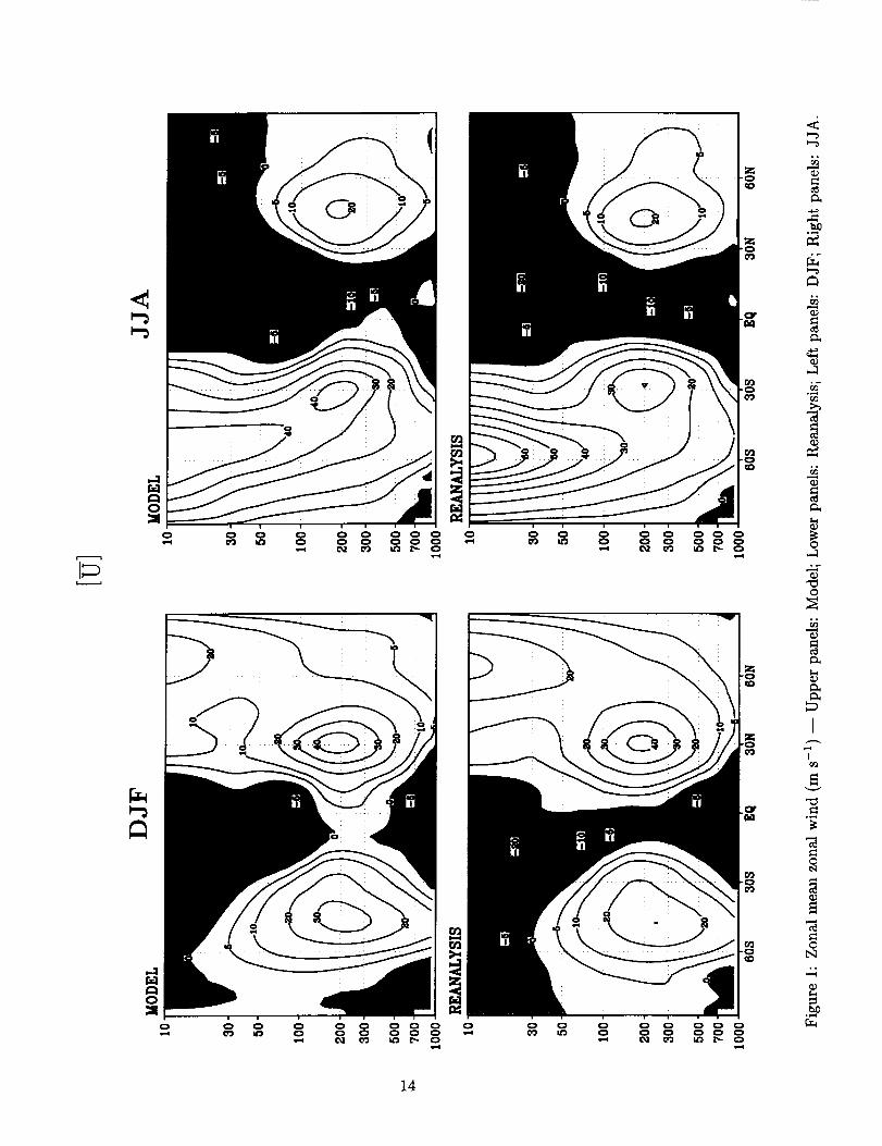
Zonal mean zonal wind (m s -I) -- Upper panels: Model; Lower panels:

Reanalysis; Left panels: DJF; Right panels: JJA ...............

2 Zonal mean zonal wind (m S -1) -- Upper panels: Model; Lower panels:

Reanalysis; Left panels: MAM; Right panels: SON ..............

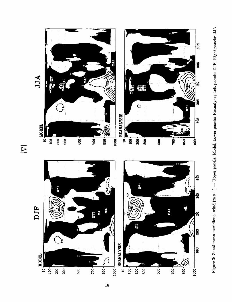
Zonal mean meridional wind (m s -1) -- Upper panels: Model; Lower panels:


7

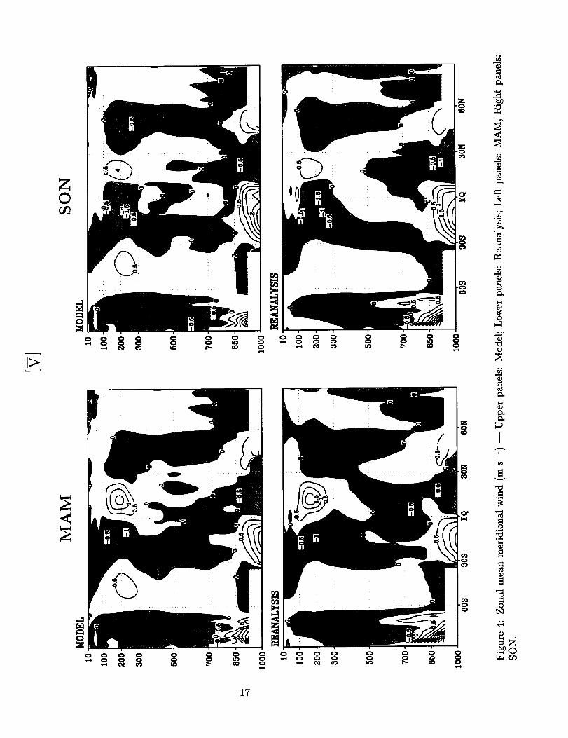
Zonal mean meridional wind (m s-1) -- Upper panels: Model; Lower panels:


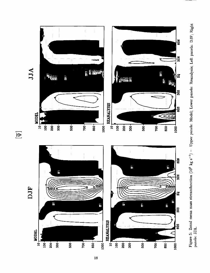
Zonal mean mass streamfunction (109 kg s -1) -- Upper panels: Model; Lower

panels: Reanalysis; Left panels: DJF; Right panels: JJA ...........

Zonal mean mass streamfunction (109 kg s -1) -- Upper panels: Model; Lower

panels: Reanalysis; Left panels: MAM; Right panels: SON ..........

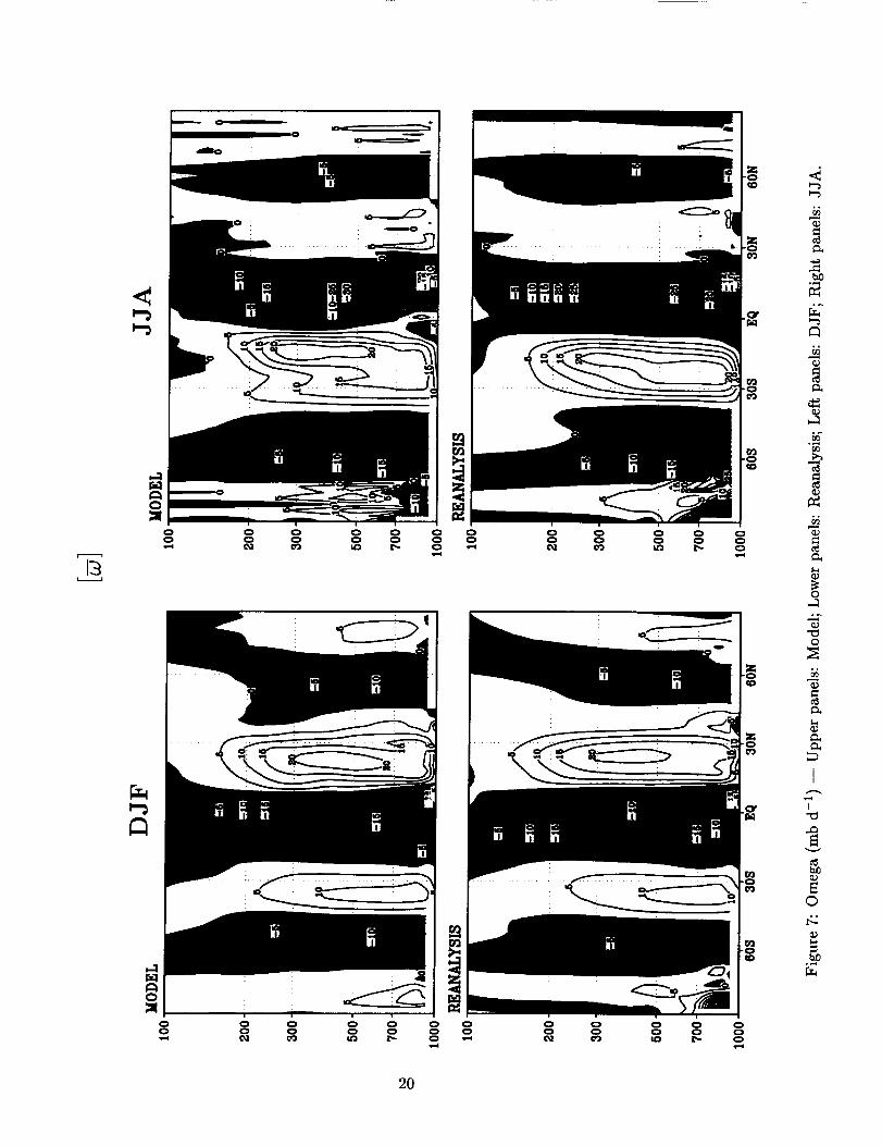
Omega (rob d -1) -- Upper panels: Model; Lower panels: Reanalysis; Left

panels: DJF; Right panels: JJA .........................

Omega (mb d -1) -- Upper panels: Model; Lower panels: Reanalysis; Left

panels: MAM; Right panels: SON ........................

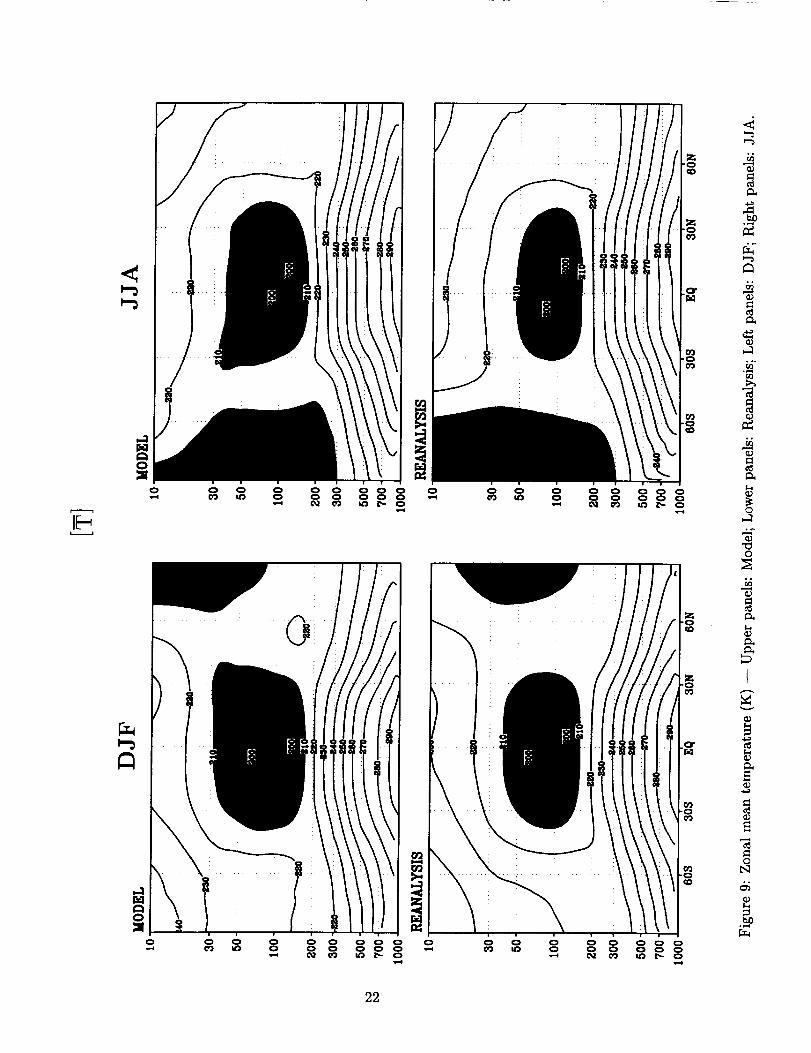
Zonal mean temperature (K) -- Upper panels: Model; Lower panels: Re-

analysis; Left panels: DJF; Right panels: JJA .................

10

11

12

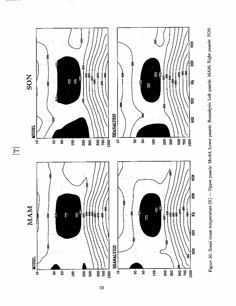
Zonal mean temperature (K) -- Upper panels: Model; Lower panels: Re-

analysis; Left panels: MAM; Right panels: SON ................

Zonal mean specific humidity (g kg -1) -- Upper panels: Model; Lower panels:


Zonal mean specific humidity (g kg -1) -- Upper panels: Model; Lower panels:


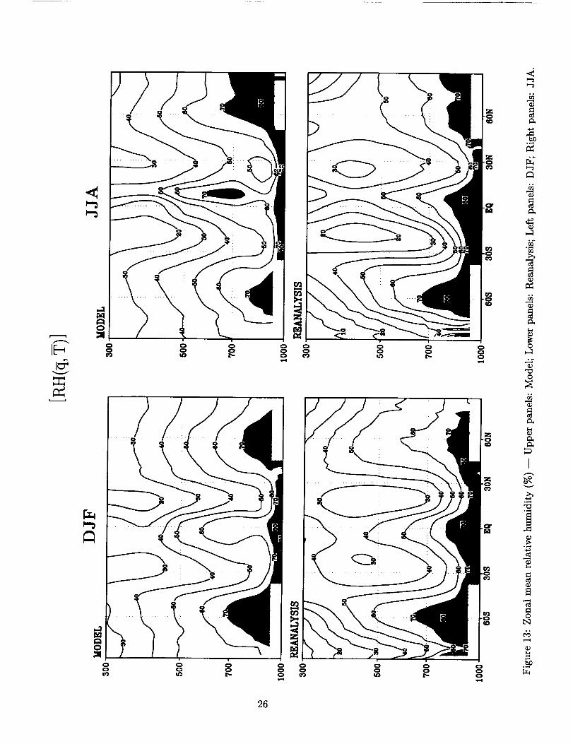
13 Zonal mean relative humidity (%) -- Upper panels: Model; Lower panels:


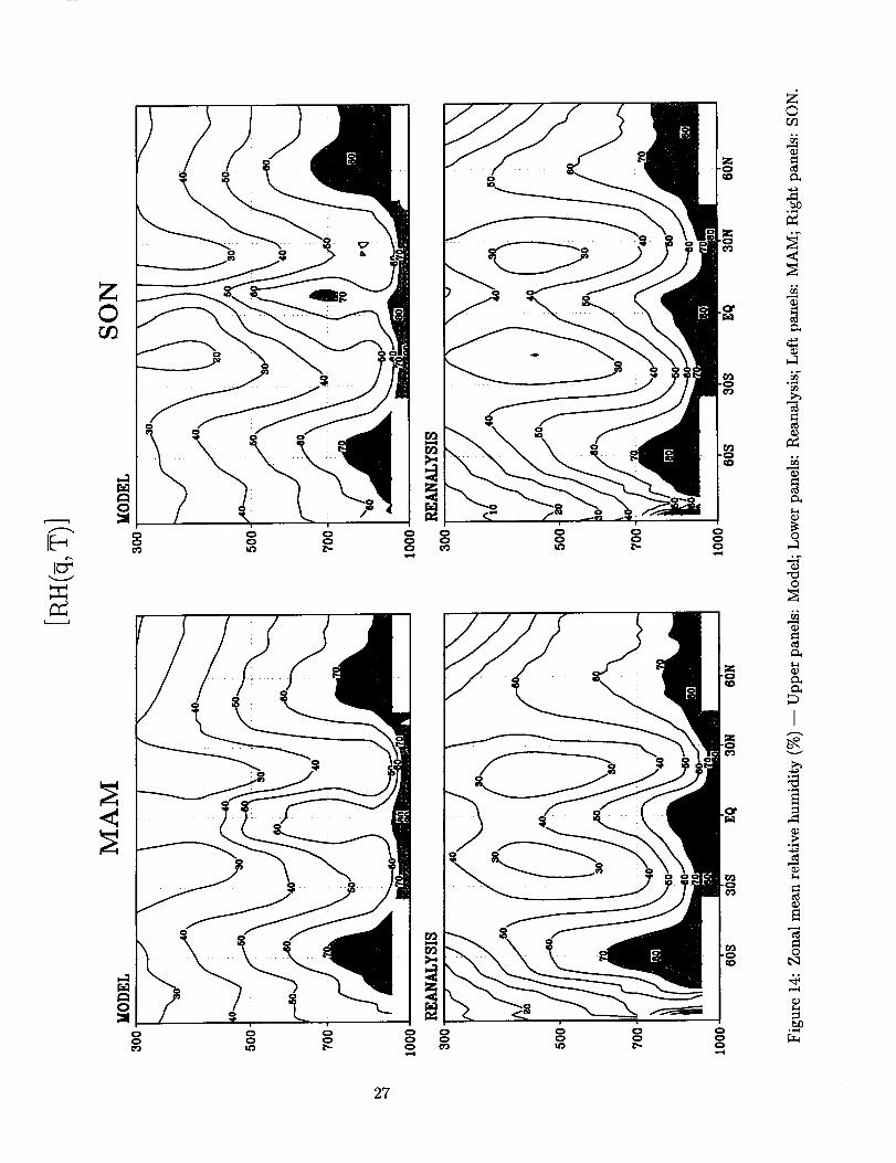
14 Zonal mean relative humidity (%) -- Upper panels: Model; Lower panels:


15 Zonal mean zonal wind bias (m s -1) ......................

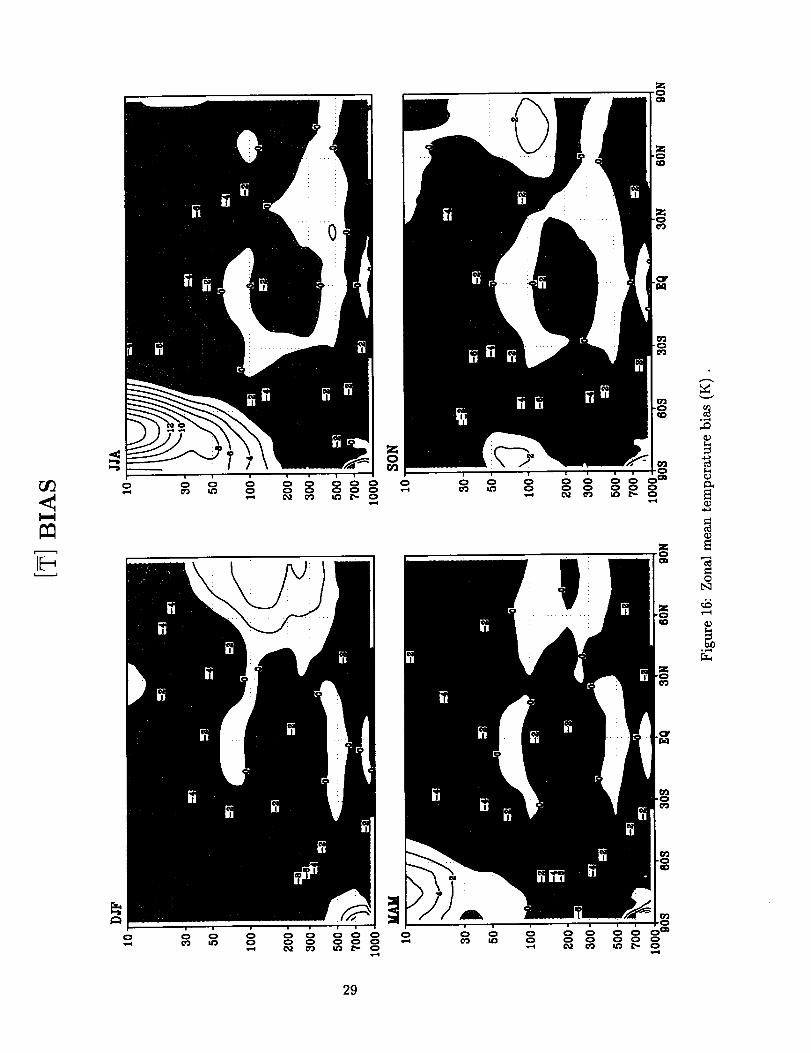
16 Zonal mean temperature bias (K) .......................

13

14

15

16

17

18

19

2O

21

22

23

24

25

26

27

28

29

vii

17 Zonalmeanspecifichumidity bias(g kg-1) .................. 30

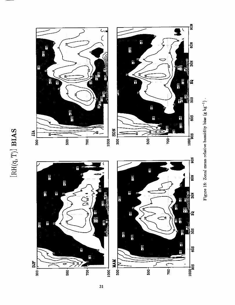
18 Zonalmeanrelativehumiditybias (g kg-1) .................. 31

GLOBAL MAPS

19 Zonal wind at 200 mb for DJF-- Top: Model, Bottom: Reanalysis. Con-

tour interval: 5 m s -1. Easterlies indicated by dark shading, light shading-1indicates westerlies in excess of 40 m s ....................

2O Zonal wind at 200 mb for JJA-- Top: Model, Bottom: Reanalysis. Con-

tour interval: 5 m s -1. Easterlies indicated by dark shading, light shading-1indicates westerlies in excess of 40 m s ....................

21 Zonal wind at 200 mb for MAM-- Top: Model, Bottom: Reanalysis. Con-

tour interval: 5 m s -1. Easterlies indicated by dark shading, light shadingindicates westerlies in excess of 40 m s -1 ....................

22 Zonal wind at 200 mb for SON-- Top: Model, Bottom: Reanalysis. Con-

tour interval: 5 m s -1. Easterlies indicated by dark shading, light shadingindicates westerlies in excess of 40 m s -1 ....................

23 Zonal wind at 850 mb for DJF-- Top: Model, Bottom: Reanalysis. Contourinterval: 3 m s -1. Easterlies are shaded .....................

24 Zonal wind at 850 mb for JJA-- Top: Model, Bottom: Reanalysis. Contourinterval: 3 m s -1. Easterlies are shaded .....................

25 Zonal wind at 850 mb for MAM-- Top: Model, Bottom: Reanalysis. Contourinterval: 3 m s-1. Easterlies are shaded .....................

26 Zonal wind at 850 mb for SON-- Top: Model, Bottom: Reanalysis. Contourinterval: 3 m s -1. Easterlies are shaded .....................

27 ;ea-level pressure for DJF-- Top: Model, Bottom: Reanalysis. Contour

interval: 4 mb. Shading indicates pressures in excess of 1000 mb .......

28 Sea-level pressure for JJA-- Top: Model, Bottom: Reanalysis. Contour


29 Sea-level pressure for MAM-- Top: Model, Bottom: Reanalysis. Contour


30 Sea-level pressure for SON-- Top: Model, Bottom: Reanalysis. Contour


31 Eddy geopotential height at 300 mb for DJF-- Top: Model, Bottom: Re-

analysis. Contour interval: 40 m. Shading indicates negative values .....

33

34

35

36

37

38

39

4O

41

42

43

44

45

46

°°°

VIII

32

33

34

35

36

37

38

39

4O

41

42

43

44

45

46

47

48

49

Eddy geopotential height at 300 mb for JJA-- Top: Model, Bottom: Re-


Eddy geopotential height at 300 mb for MAM-- Top: Model, Bottom: Re-


Eddy geopotential height at 300 mb for SON-- Top: Model, Bottom: Re-


Omega at 500 mb (mb d -1) for DJF-- Top: Model, Bottom: Reanalyms.

Contour interval: 4 mb d -1. Shading indicates rising motion .........

Omega at 500 mb (mb d -1) for JJA-- Top: Model, Bottom: Reanalysls.

Contour interval: 4 mb d -1. Shading indicates rising motion .........

Omega at 500 mb (rob d -1)Contour interval: 4 mb d -1.

Omega at 500 mb (mb d -1)Contour interval: 4 mb d -1.

for MAM-- Top: Model, Bottom: Reanalysls.

Shading indicates rising motion .........

for SON-- Top: Model, Bottom: Reanalysls.

Shading indicates rising motion .........

Eddy stream function at 200 mb for DJF-- Top: Model, Bottom: Reanalysls.Contour interval: 5 x 10 6 m 2 s -1. Shading indicates negative values .....

Eddy stream function at 200 mb for JJA-- Top: Model, Bottom: Reanalysls.Contour interval: 5 x 10 6 m 2 s -1. Shading indicates negative values .....

Eddy stream function at 200 mb for MAM-- Top: Model, Bottom: Reanal-

ysis. Contour interval: 5 x 10 6 m 2 s -1. Shading indicates negative values.

Eddy stream function at 200 mb for SON-- Top: Model, Bottom: Reanalysis.Contour interval: 5 x 106 m 2 s -1. Shading indicates negative values .....

Velocity potential at 200 mb for DJF-- Top: Model, Bottom: Reanalysis.

Contour interval: 5 x 106 m 2 s -1. Shading indicates negative values .....

Velocity potential at 200 mb for JJA-- Top: Model, Bottom: Reanalysis.


Velocity potential at 200 mb for MAM-- Top: Model, Bottom: Reanalysis.


Velocity potential at 200 mb for SON-- Top: Model, Bottom: Reanalysis.

Contour interval: 5 × 106 m 2 s -1. Shading indicates negative values .....

Zonal mean sea-level pressure (mb) Solid: Model, Dashed:Reanalysis ....

Zonal mean zonal wind at 200 mb (m s -1) Solid: Model, Dashed:Reanalysis.

Zonal mean zonal wind at 850 mb (m s-1) Solid: Model, Dashed:Reanalysis.

47

48

49

5O

51

52

53

54

55

56

57

58

59

6O

61

62

63

64

ix

ZONAL MEAN STATISTICS 65

5O Zonal mean eddy standard deviation of u (m s -1) for DJF-- Upper panels:

Model; Lower panels: Reanalysis; Left panels: Transients; Right panels:

Stationary .....................................

51 Zonal mean eddy standard deviation of u (m s -1) for JJA-- Upper panels:

Model; Lower panels: Reanalysis; Left panels: Transients; Right panels:Stationary .....................................

52 Zonal mean eddy standard deviation of u (m s -1) for MAM-- Upper panels:


Stationary .....................................

53 Zonal mean eddy standard deviation of u (m s -1) for SON-- Upper panels:


54 Zonal mean eddy standard deviation of v (m s -I) for DJF-- Upper panels:

Model; Lower panels: Reanalysis; Left panels: Transients; Right panels:Stationary. ....................................

55 Zonal mean eddy standard deviation of v (ms -1) for JJA-- Upper panels:


Stationary .....................................

56 Zonal mean eddy standard deviation of v (m s -1) for MAM-- Upper panels:


57 Zonal mean eddy standard deviation of v (m S -1) for SON-- Upper panels:


Stationary .....................................

58 Zonal mean eddy kinetic energy (m 2 s -2) for DJF-- Upper panels: Model;

Lower panels: Reanalysis; Left panels: Transients; Right panels: Stationary.

59 Zonal mean eddy kinetic energy (m 2 s -2) for JJA-- Upper panels: Model;


60 Zonal mean eddy kinetic energy (m 2 s -2) for MAM-- Upper panels: Model;


61 Zonal mean eddy kinetic energy (m 2 s -2) for SON-- Upper panels: Model;


62 Zonal mean standard deviation of w (mb d -1) for DJF-- Upper panels:


66

67

68

69

7O

71

72

73

74

75

76

77

78

x

63 Zonal mean standard deviation of w (mb d -1) for JJA-- Upper panels:


Stationary. .................................... 79

64 Zonal mean standard deviation of w (mb d -1) for MAM-- Upper panels:


Stationary. .................................... 80

65 Zonal mean standard deviation of w (mb d -1) for SON-- Upper panels:


Stationary. .............................. , ..... 81

66 Zonal mean standard deviation of T (K) for DJF-- Upper panels: Model;

Lower panels: Reanalysis; Left panels: Transients; Right panels: Stationary. 82

67 Zonal mean standard deviation of T (K) for JJA-- Upper panels: Model;


68 Zonal mean standard deviation of T (K) for MAM-- Upper panels: Model;


69 Zonal mean standard deviation of T (K) for SON-- Upper panels: Model;


70 Zonal mean standard deviation of Z (m) for DJF-- Upper panels: Model;


71 Zonal mean standard deviation of Z (m) for JJA-- Upper panels: Model;


72 Zonal mean standard deviation of Z (m) for MAM-- Upper panels: Model;


73 Zonal mean standard deviation of Z (m) for SON-- Upper panels: Model;


74 Zonal mean eddy momentum transports (m 2 s -2) for DJF-- Upper panels:


Stationary. .................................... 90

75 Zonal mean eddy momentum transports (m 2 s -2) for JJA-- Upper panels:


Stationary. .................................... 91

76 Zonal mean eddy momentum transports (m 2 s -2) for MAM-- Upper panels:


Stationary. .................................... 92

xi

77 Zonalmeaneddymomentumtransports(m 2 S-2) for SON-- Upper panels:


Stationary ..................................... 93

78 Zonal mean eddy meridional heat transports (m s-1 K) for DJF-- Upper

panels: Model; Lower panels: Reanalysis; Left panels: Transients; Rightpanels: Stationary ................................ 94

79 Zonal mean eddy meridional heat transports (m s -1 K) for JJA-- Upper


8O Zonal mean eddy meridional heat transports (m s -1 K) for MAM-- Upper


81 Zonal mean eddy meridional heat transports (m s -1 K) for SON-- Upper

panels: Model; Lower panels: Reanalysis; Left panels: Transients; Right

panels: Stationary ................................ 97

82 Zonal mean eddy vertical heat transports (mb d -1 K). for DJF-- Upper


83 Zonal mean eddy vertical heat transports (rob d -1 K). for JJA-- Upper



84 Zonal mean eddy vertical heat transports (mb d -1 K). for MAM-- Upper



85 Zonal mean eddy vertical heat transports (mb d -1 K). for SON-- Upper


86 Zonal mean eddy meridional moisture transports (m s -1 g kg -1) for DJF--

Upper panels: Model; Lower panels: Reanalysis; Left panels: Transients;

Right panels: Stationary ............................. 102

87 Zonal mean eddy meridional moisture transports (m s -1 g kg -1) for JJA--

Upper panels: Model; Lower panels: Reanalysis; Left panels: Transients;

Right panels: Stationary ............................. 103

88 Zonal mean eddy meridional moisture transports (m s -1 g kg -1) for MAM--

Upper panels: Model; Lower panels: Reanalysis; Left panels: Transients;Right panels: Stationary ............................. 104

xii

89

9O

91

92

93

94

95

96

97

Zonal meaneddymeridionalmoisturetransports(m s-1 g kg-1) for SON--Upper panels: Model; Lowerpanels: Reanalysis;Left panels:Transients;Right panels:Stationary............................. 105

Verticalmeantransienteddykineticenergy(m2 s-2). Solid: Model, Dashed:Reanalysis.

106

Square root of the vertical mean [(w02] (mb d -1) Solid: Model, Dashed:Reanalysis.107

Square root of the vertical mean [(T') 2] (K) Solid: Model, Dashed:Reanalysis. 108

Square root of the vertical mean [(Z') 2] (m) Solid: Model, Dashed:Reanalysis. 109

Vertical mean [u-'_V](m 2 s -2) Solid: Model, Dashed:Reanalysis ........ 110

Vertical mean [v-7_T_] (m s-1 K) Solid: Model, Dashed:Reanalysis ...... 111

Vertical mean [w'T'] (mb d -1 K) Solid: Model, Dashed:Reanalysis ..... 112

Vertical mean [v-_] (m s-1 g kg -1) Solid: Model, Dashed:Reanalysis .... 113

GLOBAL MAPS OF SELECTED STATISTICS

98

99

100

101

102

103

104

115

interval:

interval:

interval:

2]interval:

interval:

interval:

interval:

at 200mb for DJF-- Top: Model, Bottom: Reanalysis. Contour

2 m s -1. Shading indicates values exceeding 6 m s -1 ........ 116

at 200mb for JJA-- Top: Model, Bottom: Reanalysis. Contour


at 200mb for MAM-- Top: Model, Bottom: Reanalysis. Contour

2 m s-1. Shading indicates values exceeding 6 m s-1 ........ 118

at 200mb for SON-- Top: Model, Bottom: Reanalysis. Contour


at 200mb for DJF-- Top: Model, Bottom: Reanalysis. Contour

2 m s-1. Shading indicates values exceeding 6 m s -1 ........ 120

at 200mb for JJA-- Top: Model, Bottom: Reanalysis. Contour


at 200mb for MAM-- Top: Model, Bottom: Reanalysis. Contour


xiii

105

106

107

108

109

110

111

112

113

114

115

116

117

118

119

120

V_(V') 2] at 200mb for SON-- Top: Model, Bottom: Reanalysis. Contour

interval: 2 m s -1. Shading indicates values exceeding 6 m s -1 ........ 123

_L + (v') 2] at 200mb for DJF-- Top: Model, Bottom: Reanalysis. Con-

tour interval: 30 m 2 s -2. Shading indicates values exceeding 120 m 2 s-2. . . 124

½[(u') 2 + (v') 2] at 200mb for JJA-- Top: Model, Bottom: Reanalysis. Con-

tour interval: 30 m 2 s -2. Shading indicates values exceeding 120 m 2 s -2. . . 125

1 r(u,)2 + (v,)2] at 200mb for MAM-- Top: Model, Bottom: Reanalysis. Con-_ttour interval: 30 m 2 s -2. Shading indicates values exceeding 120 m 2 s -2. . . 126

½[(u') 2 + (v') 2] at 200mb for SON-- Top: Model, Bottom: Reanalysis. Con-

tour interval: 30 m 2 s -2. Shading indicates values exceeding 120 m 2 s -2. . . 127

Vf_W_) 2] at 500rob for DJF-- Top: Model, Bottom: Reanalysis. Contour

interval: 20 mb d -1. Shading indicates values exceeding 120 mb d -1 ..... 128

V/[(w') 2] at 500rob for JJA-- Top: Model, Bottom: Reanalysis. Contour


V_(W_) 2] at 500rob for MAM-- Top: Model, Bottom: Reanalysis. Contour


V/[(w') ] at 500rob for SON-- Top: Model, Bottom: Reanalysis. Contour


v_(T') 2] at 850rap (K) for DJF-- Top: Model, Bottom: Reanalysis. Contour

interval: 1 K. Shading indicates values exceeding 4 K ............. 132

v_(T') 2] at 850mp (K) for JJA-- Top: Model, Bottom: Reanalysis. Contour

mterval: 1 K. Shading indicates values exceeding 4 K ............. 133

_at 850mp (K) for MAM-- Top: Model, Bottom: Reanalysis. Con-

tour interval: 1 K. Shading indicates values exceeding 4 K .......... 134

V/[(T') 2] at 850mp (K) for SON-- Top: Model, Bottom: Reanalysis. Contour

interval: 1 K. Shading indicates values exceeding 4 K ............. 135

_/[(Z') 2] at 200 mb (m) for DJF-- Top: Model, Bottom: Reanalysis. Contour

interval: 20 m. Shading indicates values exceeding 100 m ........... 136

V/_(Z_) 2] at 200 mb (m) for JJA-- Top: Model, Bottom: Reanalysis. Contour

interval: 20 m. Shading indicates values exceeding 100 m ........... 137

V/_(Z_) 2] at 200 mb (m) for MAM-- Top: Model, Bottom: Reanalysis. Con-

tour interval: 20 m. Shading indicates values exceeding 100 m ........ 138

xiv

_/_Z') 2] at 200mb (m) for SON-- Top: Model, Bottom: Reanalysis.Con-121tour interval: 20m. Shadingindicatesvaluesexceeding100m........ 139

122 _/_X_)2] at 200mbfor DJF-- Top: Model, Bottom: Reanalysis.Contourinterval: 2 ×106m2 s -1. Shading indicates values exceeding 8 ×106 m 2 s -1. 140

123 V/_(X') 2] at 200mb for JJA-- Top: Model, Bottom: Reanalysis. Contour

interval: 2 ×106 m 2 s -1. Shading indicates values exceeding 8 ×106 m 2 s -1. 141

124 V/_(Xr) 2] at 200mb for MAM-- Top: Model, Bottom: Reanalysis. Contour

interval: 2 × 106 m 2 s -1. Shading indicates values exceeding 8 x 106 m 2 s -1. 142

125 V/[(X_) 2] at 200mb for SON-- Top: Model, Bottom: Reanalysis. Contour

interval: 2 xl0 s m 2 s -1. Shading indicates values exceeding 8 ×10 6 m 2 s -1. 143

126 [u-_v_] at 200 mb for DJF-- Top: Model, Bottom: Reanalysis. Contour inter-

val: 20 m 2 s -2. Shading indicates negative values ............... 144

127 [u_v _] at 200 mb for JJA-- Top: Model, Bottom: Reanalysis. Contour inter-val: 20 m 2 s -2. Shading indicates negative values ............... 145

128 [u_v _] at 200 mb for MAM-- Top: Model, Bottom: Reanalysis. Contourinterval: 20 m 2 s -2. Shading indicates negative values ............ 146

129 [u_v _] at 200 mb for SON-- Top: Model, Bottom: Reanalysis. Contourinterval: 20 m 2 s -2. Shading indicates negative values ............ 147

130 [v--7_T_] at 850 mb for DJF-- Top: Model, Bottom: Reanalysis. Contourinterval: 5 m s -1 K. Shading indicates negative values ............ 148

131 [v-7_T_] at 850 mb for JJA-- Top: Model, Bottom: Reanalysis. Contour inter-val: 5 m s -1 K. Shading indicates negative values ............... 149

132 [v_T _] at 850 mb for MAM-- Top: Model, Bottom: Reanalysis. Contourinterval: 5 m s -1 K. Shading indicates negative values ............ 150

133 [v--_-TT_] at 850 mb for SON-- Top: Model, Bottom: Reanalysis. Contourinterval: 5 m s -1 K. Shading indicates negative values ............ 151

134 -[w-_-TT_] at 850 mb for DJF-- Top: Model, Bottom: Reanalysis. Contourinterval: 50 mb d -1 K. Shading indicates downward heat transport ..... 152

135 -[w--T_T_] at 850 mb for JJA-- Top: Model, Bottom: Reanalysis. Contourinterval: 50 mb d -1 K. Shading indicates downward heat transport ..... 153

136 -[w_T _] at 850 mb for MAM-- Top: Model, Bottom: Reanalysis. Contour

interval: 50 mb d -1 K. Shading indicates downward heat transport ..... 154

xv

137

138

139

140

141

-[w'T'] at 850 mb for SON-- Top: Model, Bottom: Reanalysis. Contour

interval: 50 mb d -1 K. Shading indicates downward heat transport ..... 155

[v--_] at 850 mb (m s -1 g kg -1) for DJF-- Top: Model, Bottom: Reanalysis.

Contour interval: 2 m s -1 g kg -1. Shading indicates negative values .... 156

[v'q'] at 850 mb (ms -1 g kg -1) for JJA-- Top: Model, Bottom: Reanalysis.

Contour interval: 2 m s-1 g kg -1. Shading indicates negative values .... 157

[v-_] at 850 mb (ms -1 g kg -1) for MAM-- Top: Model, Bottom: Reanalysis.


[v--_] at 850 mb (ms -1 g kg -1) for SON-- Top: Model, Bottom: Reanalysis.


GLOBAL MAPS OF PHYSICS DIAGNOSTICS 161

142 Total precipitation (ram d-l). The comparison is for the entire 20-year period

of the run. -- Upper panels: Model; Lower panels: Reanalysis; Left panels:DJF; Right panels: JJA ............................. 162

143 Total precipitation (mm d-l). The comparison is for the entire 20-year period

of the run. -- Upper panels: Model; Lower panels: Reanalysis; Left panels:MAM; Right panels: SON ............................ 163

144 Total precipitable water (kg m-2). The comparison is for the period July

1987 to February 1992. -- Upper panels: Model; Lower panels: Reanalysis;

Left panels: DJF; Right panels: JJA. Contour interval: 10 kg m -2. Shading

indicates values in excess of 30 kg m -2 ..................... 164

145 Total precipitable water (kg m-2). The comparison is for the period July 1987

to February 1992. -- Upper panels: Model; Lower panels: Reanalysis; Left

panels: MAM; Right panels: SON. Contour interval: 10 kg m -2. Shadingindicates values in excess of 30 kg m -2 ..................... 165

146 Outgoing longwave radiation at the top of the atmosphere (W m-2). The

comparison is for the ERBE period: January 1985 to December 1989.. Solid:

Model, Dashed: ERBE .............................. 166

147 Net downward shortwave radiation at the top of the atmosphere (W m-2).

The comparison is for the ERBE period: January 1985 to December 1989..

Solid: Model, Dashed: ERBE ........................... 167

148 Net downward radiation at the top of the atmosphere at the top of the

atmosphere (W m-2). The comparison is for the ERBE period: January

1985 to December 1989.. Solid: Model, Dashed: ERBE ............ 168

149 Longwave cloud radiative forcing (W m-2).. Solid: Model, Dashed: ERBE. 169

xvi

150

151

152

153

154

155

156

157

158

159

160

161

162

Shortwave cloud radiative forcing (W m-S). The comparison is for the ERBE

period: January 1985 to December 1989.. Solid: Model, Dashed: ERBE. 170

Net cloud radiative forcing (W m-S). The comparison is for the ERBE

period: January 1985 to December 1989.. Solid: Model, Dashed: ERBE. 171

Longwave cloud radiative forcing (W m-S). The comparison is for the ERBE

period: January 1985 to December 1989.-- Upper panels: Model; Lower

panels: Reanalysis; Left panels: DJF; Right panels: JJA ........... 172

Longwave cloud radiative forcing (W m-2). The comparison is for the ERBE


panels: Reanalysis; Left panels: MAM; Right panels: SON .......... 173













Outgoing longwave radiation bias (Model - ERBE) (W m-2). The compari-

son is for the ERBE period: January 1985 to December 1989 ........ 178

Net downward shortwave radiation bias (Model - ERBE) (W m-2). The

comparison is for the ERBE period: January 1985 to December 1989 .... 179

Net radiation bias (Model - ERBE) (W m-2). The comparison is for the

ERBE period: January 1985 to December 1989 ................ 180

Zonal component of the surface wind stress (dynes cm-2). -- Upper panels:

Model; Lower panels: Reanalysis; Left panels: DJF; Right panels: JJA.

Results from the ECMWF re-analysis are for the 10-year period December

1979 to November 1989. Model results are for all 20 years ........... 181

Zonal component of the surface wind stress (dynes cm-2). -- Upper panels:

Model; Lower panels: Reanalysis; Left panels: MAM; Right panels: SON.

Results from the ECMWF re-analysis are for the 10-year period December

1979 to November 1989. Model results are for all 20 years ........... 182

xvii

163

164

165

166

167

168

169

170

Meridional componentof the surfacewind stress(dynescm-2). -- Upperpanels:Model; Lowerpanels:Reanalysis;Left panels:DJF; Right panels:JJA. Resultsfrom the ECMWF re-analysisare for the 10-yearperiodDe-cember1979to November1989.Modelresultsare for all 20years...... 183

Meridional componentof the surfacewind stress (dynes cm-2). -- Upper

panels: Model; Lower panels: Reanalysis; Left panels: MAM; Right pan-

els: SON. Results from the ECMWF re-analysis axe for the 10-year period

December 1979 to November 1989. Model results are for all 20 years ..... 184

Curl of the surface wind stress (10 -6 N m-3). -- Upper panels: Model; Lower

panels: Reanalysis; Left panels: DJF; Right panels: JJA. Results from the

ECMWF re-analysis are for the 10-year period December 1979 to November

1989. Model results are for all 20 years ..................... 185

Curl of the surface wind stress (10 -6 N m-3). -- Upper panels: Model;

Lower panels: Reanalysis; Left panels: MAM; Right panels: SON. Results

from the ECMWF re-analysis are for the 10-year period December 1979 to

November 1989. Model results are for all 20 years ............... 186

Surface sensible heat flux (W m-2). -- Upper panels: Model; Lower panels:

Reanalysis; Left panels: DJF; Right panels: JJA. Results from the ECMWF

re-analysis are for the 10-year period December 1979 to November 1989.

Model results are for all 20 years ......................... 187

Surface sensible heat flux (W m-2). -- Upper panels: Model; Lower pan-

els: Reanalysis; Left panels: MAM; Right panels: SON. Results from the



Surface latent heat flux (W m-2). -- Upper panels: Model; Lower panels:

Reanalysis; Left panels: DJF; Right panels: JJA. Results from the ECMWF

re-analysis are for the 10-year period December 1979 to November 1989.

Model results are for all 20 years ......................... 189

Surface latent heat flux (W m-2). -- Upper panels: Model; Lower pan-

els: Reanalysis; Left panels: MAM; Right panels: SON. Results from the



xviii

1 Introduction

The mission of the NASA Seasonal-to-Interannual Prediction Project (NSIPP) is to use

remotely-sensed observations to enhance the predictability of E1 Nino/Southern Oscillation

(ENSO) and other major seasonal-to-interannual signals and their global teleconnections.

Fullfilling this mission requires state-of-the-art general circulation models of the coupled

ocean-atmosphere-land system that can be used to assimilate observations and to demon-

strate the utility of those observations through experimental prediction.

This report presents the climate characteristics of version 1 of the NSIPP Atmospheric Gen-

eral Circulation Model (the NSIPP 1 AGCM). This model, which is the atmosphere/land

component of the full coupled atmosphere-land-ocean model, is currently being used in a

wide range of atmospheric, coupled ocean/atmosphere and land/atmosphere simulation and

predictability studies. Subsequent reports will summarize the predictability characteristics

and interannual variability of this version of the AGCM.

The NSIPP AGCM was developed at Goddard. NSIPP 1 is a production version of the

development cycle Aries l_l/Patch 4. We note that the Goddard Earth Observing System

(GEOS) model currently being used by the Data Assimilation Office (DAO) stems from

the same development path. The GEOS model was, however, tailored for atmospheric data

assimilation, while the NSIPP model was developed for climate simulation and prediction.

This difference in application manifests itself largely in the tailoring and tuning of the

physical parameterizations to ensure that certain key aspects of the atmosphere/land system

are faithfully reproduced by the model. For example, in the development of the NSIPP

AGCM, much attention has been devoted to the simulation of wind stresses over the tropical

Pacific Ocean in order to obtain the proper atmosphere-ocean coupling when run in a

coupled mode. Also, the middle latitude atmospheric stationary waves must be sufficiently

unbiased in order to obtain the proper extratropical ENSO response and its variability

(e.g., Schubert et al. 2000). In fact, it is these two aspects of the model climatology that

motivated the recent model development, leading to Patch 4.

Although one may regard most changes in Patch 4 as fairly minor, they led to a much

improved simulation over earlier versions. These changes include an increase in vertical

resolution from 22 to 34 levels, with all new levels added near the surface; a modified

version of the convection parameterization, with a more complete liquid water budget in

updrafts; a modified version of the turbulence scheme, together with the elimination of dry

convective adjustment; the use of filtered topography; and some minor modifications to the

cloud disgnostic scheme. More details are presented in the next section.

The results presented are from a 20-year (December 1979-November 1999) "AMIP-style"

integration of the NSIPP 1 AGCM. Here AMIP indicates that the model was run with

monthly mean sea surface temperature and sea ice specified from observations following the

experimental design of the Atmospheric Model Intercomparison Project (Gates 1992). The

results are compared with the reanalysis performed by the National Centers for Environ-

mental Prediction and the National Center for Atmospheric Research (the NCEP/NCAR

Reanalysis, Kalnay et al., 1995) for the same time period. Other verification data include

the European Center for Medium-Range Weather Foreacsting (ECMWF) reanalysis (Gibson

et al., 1996), Special Sensor Microwave/Imager (SSM/I) total precipitable water, Xie arts

Arkin (1997)estimatesof precipitation,and Earth RadiationBudgetExperiment(ERBE)measurementsof shortwaveandlongwaveradiation.

The atlas is organizedby season.The basicquantitiesincludeseasonalmeanglobalmapsand zonaland vertical averagesof circulation, variance/covariancestatistics,and selectedphysicsquantities.

Section2 describesthe NSIPP 1 AGCM. Sections3 and 4 describethe model integrationand validation data, respectively.Section5 givesan overviewof the organizationof theatlas.The resultsarediscussedin Sections6-8.

2 Description of the model

The AGCM is the atmospheric component of the NSIPP coupled prediction system. It uses

a finite-difference dynamical core based on a C-grid in the horizontal and a standard sigma

coordinate in the vertical. A detailed description of this core is given in Suarez and Takacs

(1995).

Finite differences are second-order accurate, except for advection by the rotational part of

the flow, which is done at fourth order. The momentum equations use a fourth-order version

of the enstrophy conserving scheme of Sadourney (1975). The horizontal advection schemes

for potential temperature and moisture are also fourth-order and conserve the quantity and

its square (Takacs and Suarez, 1996).

The parameterizations of solar and infrared radiative heating rates are described in Chou

and Suarez (1999) and Chou and Suarez (1994). The solar parameterization includes ab-

sorption due to 03, CO2, water vapor, 02, and clouds, as well as gaseous and aerosol

scattering. The solar spectrum is divided into eight Visible-UV bands and three near-IR

bands. A k-distribution method is used within each band. The eight VIS-UV bands use a

single k-interval, while the IR bands use ten intervals each. Effects of multiple scattering by

clouds and aerosols are treated using the $-Eddington approximation for the direct beam

and Sagan-Pollock for diffuse radiation. The infrared parameterization includes absorp-

tion by water vapor, CO2, 03, methane, N20, CFC-11, CFC-12, and CFC-22, within eight

spectral bands, but in the results prsented only water vapor, CO2, and 03 are included.

From the moist physics parameterizatious, the GCM estimates a cloud fraction at each

level. For the solar radiation calculation, the GCM levels are then grouped into three

regions which axe identified with high (a < 0.56) middle (0.56 < a < 0.77) and low (a >

0.77) clouds. Within each of these regions, clouds are assumed to be maximally overlapped

and the cloud fractions are scaled using a scheme that depends on solar zenith angle and

optical thickness. This leaves us with a single cloud fraction in each of the three regions.

The overlapping between these region is treated "exactly" by assuming random overlapping

and combining the results of full transfer calculations for the eight possible cases.

Turbulence throughout the atmospheric column is modeled using the Louis et al.(1982)

scheme. This is a local "K" scheme with Richardson number-dependent viscosity and

diffusivity. In practice, we found that the scheme contributed to excessive annual mean

stressesover the equatorialpacific, as well as to unrealistic seasonal variation of these

stresses. These deficiencies were alleviated by using a smaller than usual value for the eddy-

mixing length scale A0. We use A0--=20 meters, compared to typical values of 80 to 160 meters

in other implementations of the scheme. We also truncate mixing in the stable Ri regime, so

that for Ri>3.0 vertical viscosity and diffusivity are exactly zero. This eliminates sporadic

patches of significant momentum mixing in the middle troposphere, which we believe havean adverse effect on the simulation of surface wind stresses. These modifications to the

standard implementation of the Louis scheme do not have noticeable negative impacts on

other aspects of the model climate. We also note here that dry convective adjustment hasbeen eliminated from the current version of the model.

The model uses the gravity-wave drag parameterization described by Zhou et al. (1996).

The Zhou scheme incorporates only orographically forced gravity waves. Directional anisotropy

of the orographic forcing is ignored. The scheme contains two important "tunable" param-

eters, the effective wavenumber krnw for the waves, and a maximum surface amplitude for

the waves hrnax. These must be determined empirically. Currently we use krnw = 2.5 x 10 -5

m -1 and hmax = 400 m. The surface amplitude of waves is the lower of hmax and a

local gridbox RMS topographic deviation derived from the GTOPO30 thirty arcsecond

topographic data set (http://edcwww.cr.usgs.gov/landdaac/gtopo30/gtopo30.html). The

GTOPO30 data have been binned by averaging the heights in 5 x 5 squares to produce a

2.5' dataset. It is with these data that the RMS amplitudes are computed.

In addition to the Zhou scheme, the model incorporates enhanced Rayleigh damping above

a=0.05. This damping is formulated as

('0.05- o (0. rJ)0= "y0\ 0.05

where U is the model horizontal wind vector. The strength _'0 = (60 m s-1)-2(10 d) -1 is

chosen to damp a 60 m s-1 jet in 10 days. This drag is a crude ad hoc representation of

missing gravity wave drag in the middle atmosphere. It is intended primarily to reduce the

strength of the polar night jet in the winter stratosphere in the interest of computational

stability. This drag formulation does not produce realistic simulations of the stratosphericclimate.

We find that our simulation of stationary planetary waves improves significantly when the

topographic elevation data used by the model is first filtered to eliminate high spatial

frequencies. This is accomplished using a 12-th order Coiflet filter. Coiflets are nearly

symmetrical orthogonal wavelets with compact support and exact reconstruction. We filter

by simply removing the highest frequency (octave) of the Coiflet transform of the topography

and reconstructing. The compact support of the Coiflet filter reduces the ringing that

plagues higher-order filtering techniques.

Penetrative convection originating in the boundary layer is parameterized using the Relaxed

Arakawa-Schubert (RAS) scheme (Moorthi and Suarez, 1992), which is a simple and effi-

cient implementation of the Arakawa-Schubert scheme. The version described in Moorthi

and Suarez, RAS-1, is the standard parameterization used at Goddard. It has also been

tested at NCEP, NCAR, and COLA, and has performed particularly well in simulating the

atmospheric response to tropical SST anomalies -- a crucial aspect of the coupled predic-

tion problem. We have recently updated it by including a more detailed condensate budget

3

in the updraft. This version,whichwereferto asRAS1.5,is theoneusedin the NSIPP1AGCM.

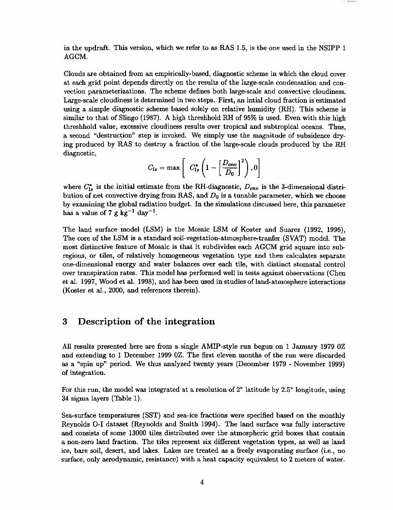
Cloudsare obtained from an empirically-based, diagnostic scheme in which the cloud cover

at each grid point depends directly on the results of the large-scale condensation and con-

vection parameterizations. The scheme defines both large-scale and convective cloudiness.

Large-scale cloudiness is determined in two steps. First, an intial cloud fraction is estimated

using a simple diagnostic scheme based solely on relative humidity (RH). This scheme is

similar to that of Slingo (1987). A high threshhold RH of 95% is used. Even with this high

threshhold value, excessive cloudiness results over tropical and subtropical oceans. Thus,

a second "destruction" step is invoked. We simply use the magnitude of subsidence dry-

ing produced by RAS to destroy a fraction of the large-scale clouds produced by the RH

diagnostic,

where C_s is the initial estimate from the RH-diagnostic, Deny is the 3-dimensional distri-bution of net convective drying from RAS, and Do is a tunable parameter, which we choose

by examining the global radiation budget. In the simulations discussed here, this parameter

has a value of 7 g kg-1 day-1.

The land surface model (LSM) is the Mosaic LSM of Koster and Suarez (1992, 1996),

The core of the LSM is a standard soil-vegetation-atmosphere-tranfer (SVAT) model. The

most distinctive feature of Mosaic is that it subdivides each AGCM grid square into sub-

regions, or tiles, of relatively homogeneous vegetation type and then calculates separate

one-dimensional energy and water balances over each tile, with distinct stomatal control

over transpiration rates. This model has performed well in tests against observations (Chen

et al. 1997, Wood et al. 1998), and has been used in studies of land-atmosphere interactions

(Koster et al., 2000, and references therein).

3 Description of the integration

All results presented here are from a single AMIP-style run begun on 1 January 1979 0Z

and extending to 1 December 1999 OZ. The first eleven months of the run were discarded

as a "spin up" period. We thus analyzed twenty years (December 1979 - November 1999)

of integration.

For this run, the model was integrated at a resolution of 2 ° latitude by 2.5 ° longitude, using

34 sigma layers (Table 1).

Sea-surface temperatures (SST) and sea-ice fractions were specified based on the monthly

Reynolds O-I dataset (Reynolds and Smith 1994). The land surface was fully interactive

and consists of some 13000 tiles distributed over the atmospheric grid boxes that contain

a non-zero land fraction. The tiles represent six different vegetation types, as well as land

ice, bare soil, desert, and lakes. Lakes are treated as a freely evaporating surface (i.e., no

surface, only aerodynamic, resistance) with a heat capacity equivalent to 2 meters of water.

Table 1: Sigma surfaces separating the 34 layers of the model.L a L a L a L a L a

1 0.000 2 0.005 3 0.010 4 0.015 5 0.0256 0.050 7 0.075 8 0.100 9 0.125 10 0.15011 0.175 12 0.200 13 0.225 14 0.275 15 0.32516 0.375 17 0.425 18 0.500 19 0.625 20 0.70021 0.750 22 0.775 23 0.800 24 0.825 25 0.85026 0.865 27 0.880 28 0.895 29 0.910 30 0.925

31 0.940 32 0.955 33 0.970 34 0.985 35 1.000

One peculiarity of this run is that, to avoid running with a sea-ice model, we have spec-

ified both sea ice fractions and temperatures. The former vary interannual, but sea-ice

temperatures repeat the same seasonal cycle each year.

4 Validation data sets

For the upper air fields and their statistics, we compare with the NCEP/NCAR Reanalysis

(Kalnay et al. 1994) averaged for the same period as the model simulation. For the

moisture field and various physics diagnostics we compare with various satellite and in

situ measurements described below.

Precipitation is compared with the combined satellite,gauge, and model estimates derived

by Xie and Arkin (1997). These data are available for the entire period of the simulation

from ftp: / / ftp.ncep.noaa.gov /pub /precip /cmap /monthly/.

Estimates of total precipitable water (TPW) are those generated by Wentz (1992) from the

Special Sensor Microwave Imager (SSM/I) measurements. The radiative transfer algorithm

uses three channels of microwave measurements (22V, 37V, 37H) and a scheme that accounts

for absorption and emission in the atmosphere and uses a surface emissivity value over

oceans appropriate for a wind-roughened sea surface. The scheme does not account for

scattering by raindrops or by frozen hydrometers and is, therefore inaccurate for high rain

rates. No data is produced over land or sea ice, because of the complexity of the surface

emissivity.

To validate the top of the atmosphere radiation budget, we compare with the Earth Ra-

diation Budget Experiment (ERBE) data collected by the ERBS, NOAA 9 and NOAA 10

satellites between November 1984 and February 1990. More information on ERBE may be

obtained at (http://asd-www.larc.nasa.gov/erbe/ASDerbe.html). We limit our comparison

to the 5-year period from 1985 through 1989.

Surface fluxes are compared with the first 10 years of the ECMWF reanalysis (Gibson et

al., 1996).

5 Organization and calculations

Unless otherwise noted, quantities presented in this report are averaged over the 20 years

of the integration. We will concentrate on seasonal means. Instantaneous values of the

simulated upper air data were saved four times daily at 0Z,6Z,12Z, and 18Z. Surface and

top-of-atmosphere (TOA) fluxes, precipitation, and cloudiness were accumulated at each

time step and saved once daily.

Results axe presented as zonal means and global maps of climatological means and sub-

monthly variance/covariance statistics. For selected quantities we also show the zonal

mean bias (departures from NCEP/NCAR reanalysis), and/or line plots of zonal means

at selected pressure levels or of vertical means. The zonal means are computed at the fol-

lowing pressure levels (1000, 925, 850, 700, 500, 400, 300, 250, 200, 150, 100, 70, 50, 30,

qnd 10 mb). While results are presented up to 10 mb, the model was not tuned to pro-

duce a very realistic stratosphere. In fact, the current values of Rayleigh friction produce

a rather strong damping on the stratosphere, resulting in unrealistically weak high latitudewesterlies and covariance statistics above about 50 rob.

The variance/covariance statistics are divided into "transient" and "stationary" compo-

nents. The "transient" statistics are computed from 6 hourly deviations from monthly

means of each year and each calendar month. Products are then taken and averaged for

each season and for the twenty years of the analysis. The "stationary" statistics are com-

puted from zonal departures of monthly means, these are then averaged for each season

and for the twenty years of the analysis. We will use overbars to denote a calendar monthlymean, so that u _ = u - _ is the monthly deviation of u, and square brackets to denote

a zonal mean, so that u* = u -_ is the zonal departure of u. Then the mean quadratic

quantities are defined as:

TRANSIENT(u,v) = {u-_vl}, STATIONARY(u,v) = {[_-'9-'1},

where the braces represent an average over the three months of each season and all years.

For all squared statistics, other than kinetic energy, we plot the square root, which is taken

after all averaging.

Section 6 discusses the climatological means and bias of upper air fields. Section 7 discusses

sub-monthly quadratic statistics, and Section 8 selected physics quantities.

6 Means of Upper Air Fields

The model produces a very good simulation of the general circulation of the troposphere,

including the zonally asymmetric flow and stationary eddy patterns. In the following dis-

cussion, we emphasize deficiencies that remain in the simulation.

The model simulation of the seasonal mean zonal mean winds is generally quite good.

Notable deficiencies include, weak high latitude stratospheric winter westerlies, an easterly

bias in the upper troposphere/lower stratosphere of the tropics, and a westerly bias in the

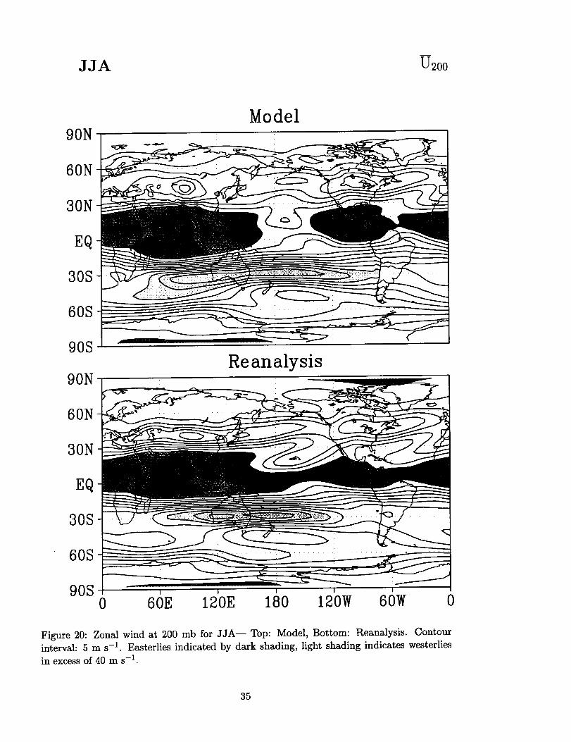
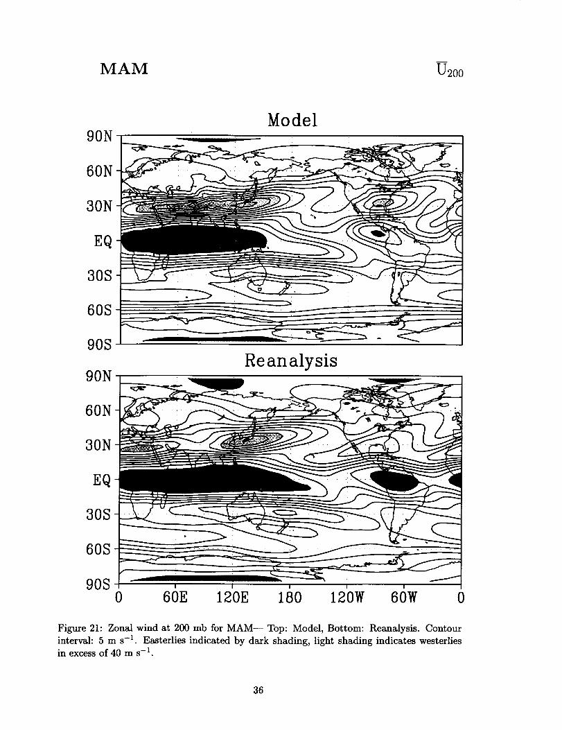
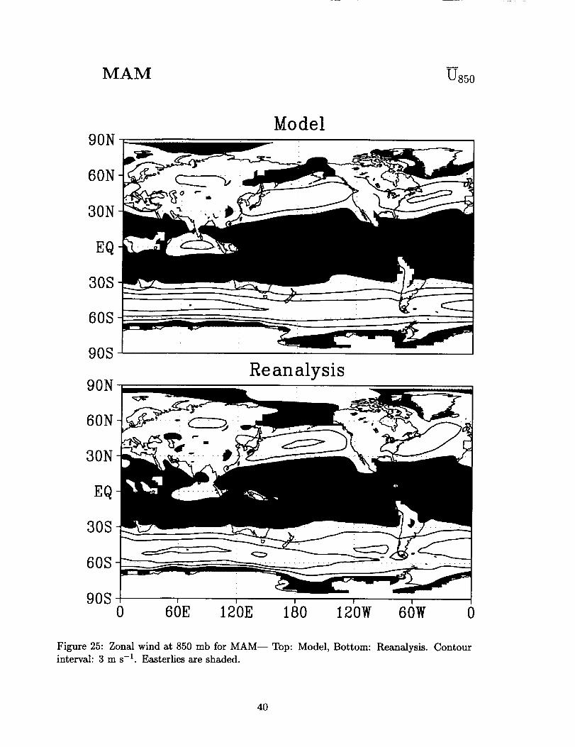
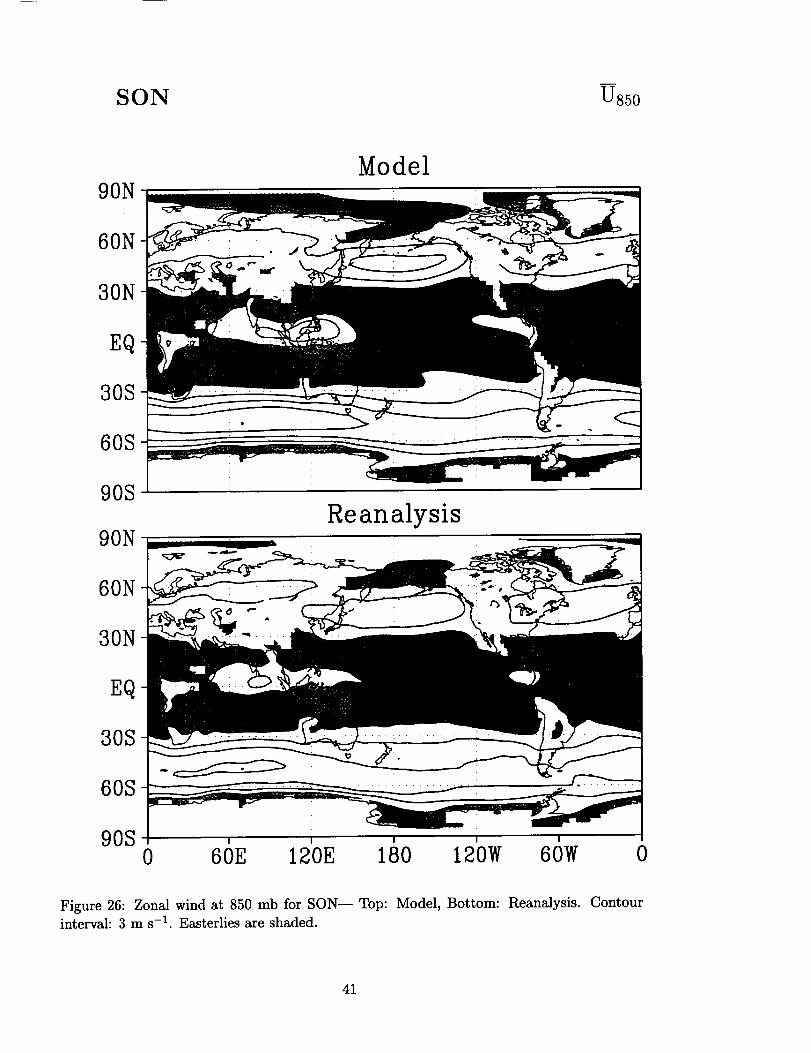
middle latitudes of the SouthernHemisphere.At 200mb, the modelproducesa westerlynodein the easterntropical Pacificthat is too strong.During JJA, the 200mb Asian andNorth Pacificjets are too weak. There is a tendencyfor a westerlybias at 200mb overthe tropical westernhemisphereduring DJF and MAM. The model fails to capture theseparationof the 200mb AfricanandEast Asianjets duringMAM. At 850mb, the modelgeneratestoo strongtropical easterliesovertheeasternPacific,andtoo strongwesterliesinthe SouthernHemispheremiddle latitudesandthe Asiansummermonsoonregion.

Theseasonalcycleof the HadleyCell is quite realistic, though the maximum rising motion

during JJA occurs substantially lower in the atmosphere (below 500 rob) than the estimates

from the NCEP/NCAR reanalysis show (400 mb). The model has a consistent cold bias

throughout most of the stratosphere, the Southern Hemisphere high latitude upper tropo-

sphere, and the tropical upper troposphere. A substantial warm bias (greater than 8 degrees

C) occurs during the winter in the stratosphere of the southern high latitudes. During all

seasons the tropical and subtropical troposphere below 800 mb is too dry (maximum bias

near 925mb), while between 700 mb and 500 mb the tropics are too wet. The moisture

bias is reflected in the relative humidity (RH) bias, though the latter also show that the

boundary layer relative humidity is too high, while away from the polar regions the upper

tropospheric relative humidity is too low.

The North Pacific and North Atlantic surface highs tend to be too strong, especially during

JJA. The North American upper tropospheric west coast ridge is too strong during DJF.

The east Asian/west Pacific trough is too weak (and has a noticeable hump) during DJF,

and it does not extend far enough into the eastern Pacific during MAM.

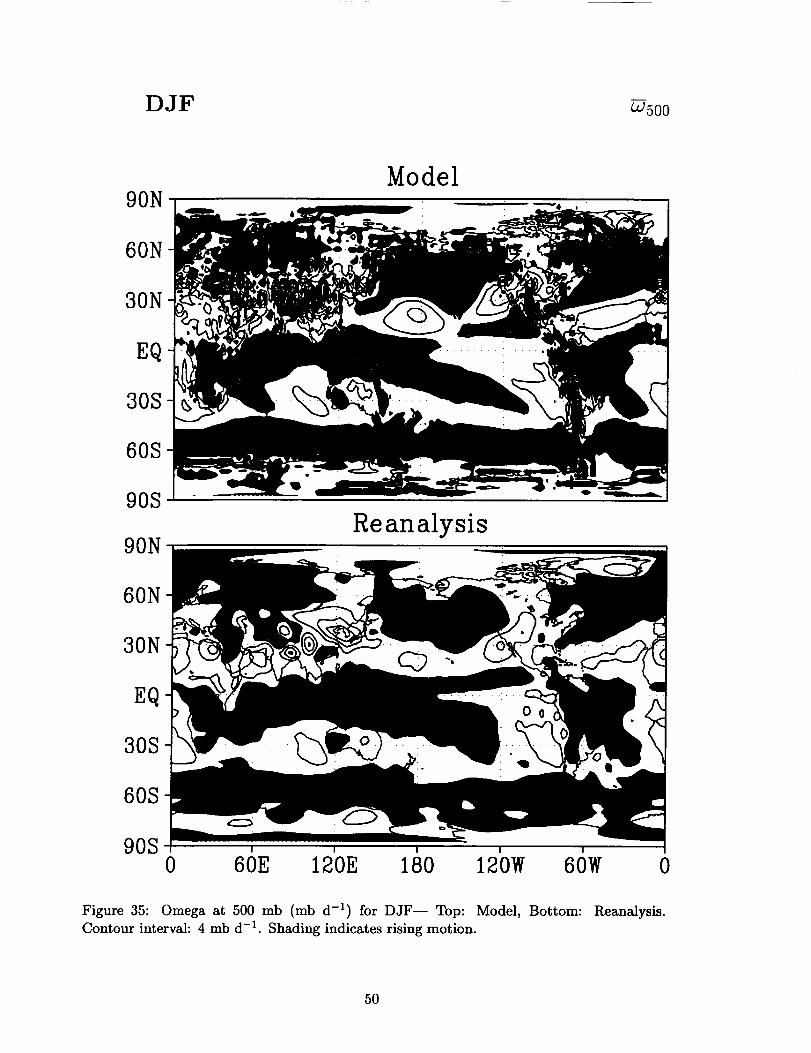
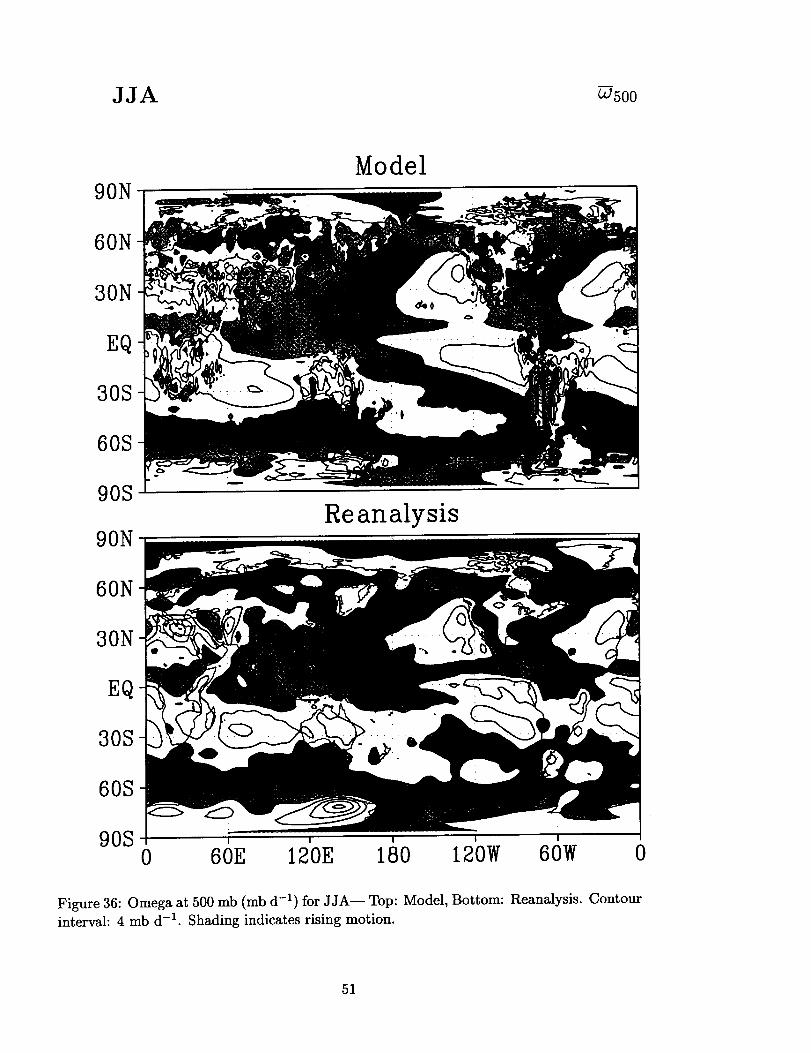
The model shows excessive noise over mountains in the 500 mb omega fields. Compared

to the NCEP reanalysis, there is insufficient rising motion over the tropical eastern Pacific

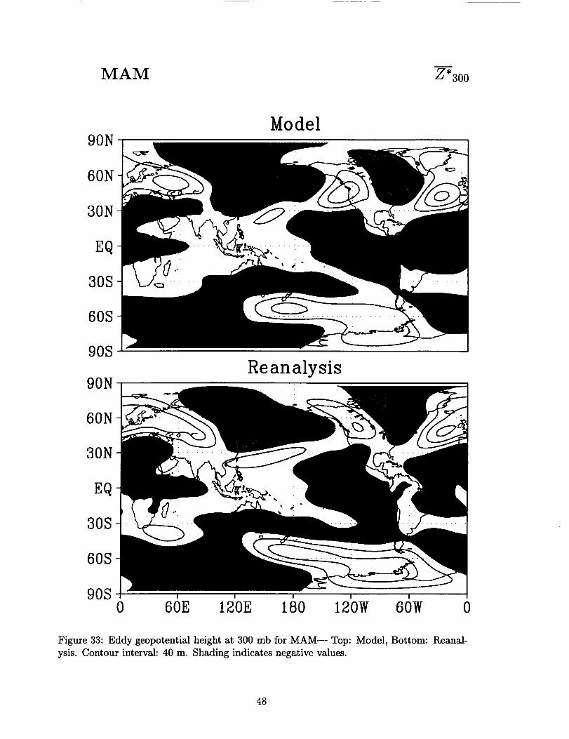
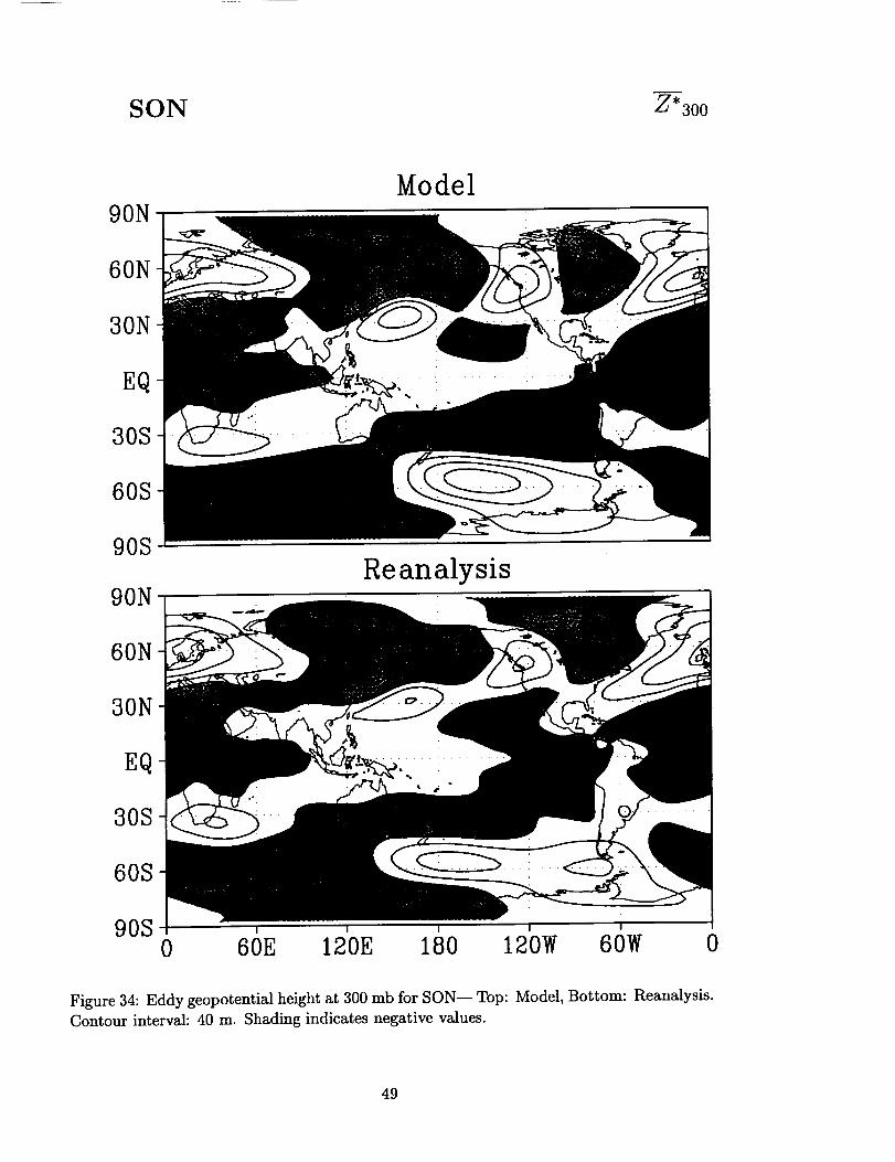
in the region of the ITCZ. The eddy stream function at 300 mb shows tropical/subtropical

stationary waves that are too weak in the eastern hemisphere, while they are too strong in

the western hemisphere during all seasons. The seasonal evolution of the 200 mb velocity

potential is quite good.

7 Sub-Monthly Quadratics of Upper Air Fields

The model produces good tropospheric transient and stationary zonal and meridonal wind

variances. However, the transient variances in both wind components (especially v) tend to

be somewhat weak in the Northern Hemisphere. This leads to a substantial underestimate

of the transient kinetic energy in the Northern Hemisphere troposphere during all seasons.

The stationary zonal wind variance is too strong in the upper tropospheric tropics. The

wind variances are much weaker than observed in the high latitudes of the stratosphere

during winter.

There are large differences in the variance of the omega field, with the model showing con-

siderably larger variance than the NCEP/NCAR reanalysis in the tropics and extratropics.

It should be noted that the quality of the reanaIysis are suspect for this field. The model

produces very good geopotential height variances in the troposphere. Similar to the wind

7

variances;however,the heightvariancesareweakerthan observedduring thecold seasonsin the highlatitudesof the stratosphere.This isespeciallysofor thestationarycomponentduring DJF in the NorthernHemisphereand during SON in the SouthernHemisphere.At 200mb, the seasonalcycleof the heightvarianceis quite good,thoughthe varianceissomewhatweakerthan observedin the NorthernHemispheremiddleand highlatitudes.

The modelproducesexcellentmeridionalfluxesof zonalmomentum.Exceptionsaxethetoo strongstationary fluxesbetween200 mb and 100 mb during JJA, and a tendencyto overestimatethe southwardtransientfluxes in the SouthernHemisphere.The modelproducesreasonableheatfluxesin thetroposphere,thoughtransientsouthwardfluxesin theSouthernHemispherearesystematicallyhigherthan in the reanalysis.In the stratosphere,thestationarymeridionalheatflux ismuchtooweakat high latitudesduringDJF, whilethetransientcomponentis too strong.The modelgeneratesveryrealisticmeridionalmoisturefluxes.

8 Surface and TOA Fluxes

The model's global precipitation distribution is much improved from that produced byearlier versions. In particular, its tendency to produce unrealistic double ITCZs in the

central and eastern Pacific has been greatly lessened. A strong vestige of the problem,however, remains in the MAM season. One of the more intractable problems with the

precipitation distribution is a "gap" in the eastern Pacific ITCZ and an associated "bull's

eye" in precipitation over Central America. This problem is apparent in all four seasons ofthe simulation.

The simulated precipitable water (vapor only) agrees quite well with the satellite estimate

(SSM/I). As might be expected, however, it shows some of the same unrealistic features as

the precipitation fields.

The zonal mean total radiation budget at the top of the atmosphere is simulated well. The

most obvious deficiency is the excessive outgoing longwave radiation at almost all latitudes

and all seasons. This results in a systematic "cold" bias in the net radiation, which is

otherwise extremely well simulated. The "cloud radiative forcings" (CRF) highlight better

the model's performance. In the OLR-CRF, the model does surprisingly well in the tropics--

a result of our improved distributions of convective activity. In the middle latitudes, the

model consistently underestimated the OLR-CRF, implying too little, or too low cloudiness

in these regions. The solar CRF is extremely good, the main problem being too weak

forcing in middle latitudes of the southern hemisphere during MAM. Aside from this, littledifferentiates it from the ERBE data.

The global distributions of CRF show clearly that some of the agreement in the zonal mean

results from a compensation of errors along latitude circles, but they also show that much of

the agreement is due to the model's improved distribution of tropical (convective) cloudiness

and of the marine stratus and stratocumulus regimes. The latter is best seen in the solarCRF distributions.

Because of its importance to the ENSO problem, we have devoted considerable attention to

the simulationof tropical surface stresses, particularly the seasonal cycle in the equatorial

Pacific. As may be seen from the global distributions shown, both the zonal and meridional

stress compare quite well with the ECMWF reanalysis. In fact, even the more difficult and

oceanographically important curl of the wind stress is very close to the reanalysis.

The same cannot be said of the sensible and latent heat fluxes, both of which the model

seems to overestimate very significantly, at least over oceans.

9 Summary

The atlas presents a very good simulation of the mean seasonal cycle of the tropospheric

general circulation. The model is shown to have very good skill in simulating the horizontal

and vertical distribution of both mean fields and variance/covariance statistics.

The results also identify a several deficiencies. Some of these, like the problems in the

eastern Pacific ITCZ, may require increased horizontal resolution. Others, however, are

things that we feel can clearly be improved within the current framework.

Nevertheless, we feel this is an acceptable model for NSIPP's purposes and have frozen it

in the form presented here. A number of other experiments have already been conducted

with it and many more will follow. These experiments address the model's sensitivity to

sea-surface temperatures, its teleconnection patterns and modes of natural variability, the

nature of its land-atmosphere interactions, and its performance in coupled integrations. In

all of these areas, the model appears to be performing quite well, and results will be reported

in the near future.

9

10

10 References

Chen, T.H. and 42 others, 1997: Cabauw experimental results from the Project for Inter-

comparison of Landsurface Parameterization Schemes (PILPS), J. Climate, 10, 1194-1215.

Chou, M.-D. and M. Suarez, 1994: An efficient thermal infrared radiation parameterization

for use in general circulation models. NASA Technical Memorandum, 104606, 10, 84pp.

Chou, M.-D. and M. J. Suarez, 1999: A solar radiation parameterization for atmospheric

studies, NASA Technical Memorandum, 104606, 11, 40pp.

Gibson,R., P.Kallberg and S. Uppsala, 1996: The ECMWF reanalysis (ERA) project.

ECMWF Newsletter, 73, 7-16.

Gates, W. L., 1992: AMIP: The atmospheric model intercomparison project. Bull. Amer.

Meteor. Soc., 73, 1962-1970.

Gruber, A. and A.F. Krueger, 1984: The status of the NOAA outgoing longwave radiation

data set. Bull. Amer. Meteor. Soc., 65, 958-962.

Kalnay, E., M. Kanamitsu, R. Kistler, W. Collins, D. Deaven, J. Derber, L. Gandin, S. Sara,

G. White, J. Woollen, Y. Zhu, M. Chelliah, W. Ebisuzaki, W. Higgins, J. Janowiak, K. C.

Mo, C. Ropelewski, J. Wang, A Leetma, R. Renolds, R Jenne, 1995: The NMC/NCAR

Reanalysis Project. Bull Amer. Meteor. Soc., 77, 437-471.

Koster, R., and M. Suarez, 1992: Modeling the land surface boundary in climate models as

a composite of independent vegetation stands. J. Geophys. Res., 97, 2697-2715.

Koster, R. and M. Suarez, 1996: Energy and Water Balance Calculations in the Mosaic

LSM, NASA Tech. Memo. 104606, Vol. 9.

Koster, R. D., M. J. Suarez, and M. Heiser, 2000: Variance and predictability of precipita-

tion at seasonal-to-interannual timescales, J. Hydrometeorology, 1, 26-41.

Louis, J., M. Tiedke, J. Geleyn, 1982: A short history of the PBL parameterization at

ECMWF. In: Proceedings, ECMWF Workshop on Planetary Boundary Layer Parameteri-

zation, Reading, UK, 59-80.

Moorthi, S. and M. Suarez, 1992: Relaxed Arakawa-Schubert: a parameterization of moist

convection for general circulation models. Mon. Weather Rev., 120, 978-1002.

Reynolds, W. R. and T. M. Smith, 1994: Improved global sea surface temperature analyses

using optimum interpolation. J. Climate, 7, 929-948.

Rossow, W. B., and R. A. Schiffer, 1991: ISCCP cloud data products. Bull. Am. Meteorol.

Soc.,72, 2-20.

Sadourney, R., 1975: The dynamics of finite difference models of the shallow water equa-

tions, J. Atmos. Sci., 32, 680-689.

11

Schubert,S.D., M. J. Suarez,Y. Changand G. Branstator,2000:Theimpactof ENSOonextratropical low frequencynoisein seasonalforecasts.Submitted to J. Climate.

Slingo, J. M., 1987: The development and verification of a cloud prediction scheme for the

ECMWF model, Q. J. R. Meteorol. Soc, 113, 899-927.

Suarez, M. J. and L. L. Takacs, 1995: Documentation of the Aries/GEOS dynamical core

Version 2, NASA Technical Memorandum 104606, 5, 58pp.

Takacs, L. L.and M. J. Suarez, 1996: Dynamical aspects of climate simulations using theGEOS GCM, NASA Technical Memorandum, 104606, 10, 56pp.

Wentz, F., 1994: User's Mannual, SSM/I Geophysical Tapes. Remote Sensing Systems, 11

pp.

Wood, E.F., and 28 others, 1998: The project for the intercomparison of land-surface

parameterization schemes (PILPS) phase 2(c) Red Arkansas river basin experiment, 1,

Experiment description and summary intercomparisons, J. Global and Planetary Change,19, 115-135.

Xie, P. and P. Arkin, 1997: Global precipitation, a 17-Year monthly analysis based on gauge

observations, satellite estimates and numerical model outputs. Bull. Am. Met. Soc., 78,2539-2558.

Zhou, J., Y. C. Sud, and K. M. Lau, 1996: Impact of orographically induced gravity wave

drag in the GLA GCM, Q. J. R. Meteorol. Soc, 122, 903-927.

12

ZONAL MEAN FIELDS

(DJF, MAM, JJA, SON)

Zonalwind

Meridionalwind

Massstreamfunction

Omega

Temperature

Specifichumidity

Relativehumidity

Zonalwind bias

Temperaturebias

Specifichumidity bias

Relativehumidity bias

13

14

0

0

0 0

0 0

Z

0

q-G

0 0 0 0 00 0 0 0 0

00

0 0 0 0 00 _ 0 0 0

J_

°_

o

I

I

o

ob_

°..._

O3

.o

0 O O 0 00 C3 0 0 0

©

°_

°_

o

I

o

Ob_

15

0

O

cO

OO

OO

OOt_

OO

O

GO

Z"O

QD

"OCr_

.g

O2

.o

_r3

.o

OOO

c_

c_

o_

O

I

o

c_

o

16

©

I>

i

00

00

0

CO

Z-0

qD

000

qJ

bOo,.._

._

_J

_J

r_

_J

o

_J

O_0_

I

I

o

_J

_J

_d

0_q

_._ °

=Z._ ©_rm

17

.zo_O

Z

03

03

bO

o_

o

I

J03

bO

c_c_

c_

o

18

'

..

o _

Z

Z

0 0 0 00 0 0 0

000v-0

0 0 0 00 0 0 0

000

._-

2_

O

_u

I

I

©

2O

©

<

21

©

I

©

o

I

oL'_

22

.<

/tll

II /

f//I

EliI

i I i

|

0

0 0 0a_ _3 0

0 0 0

0 O O O 00 0 0 O 0

.o

Z

_2

-0

_2-0

qD

O O 0 0 00 0 O 0 O

©_Q

0

I

0l'q

c_

Q;

23

°_

o

i

I

o

.°

°_

24

Z©

<

0m

00

25

i w

0 0 0 00 0 L'_ 0

°_

o

i

I

°_

oN

c_,--4

._©

J_

00

°_

o

c_

I

c_

0N

26

0 0 0 0 00 0 0 0 0

_ L_ 0

0o

oo

oo

Z

-0O_

-0_D

000

Z

.o

©

o_

o

c_

c_

o

I

v

o,.._

°_.._

c_

c_

o

_w

27

rj_ 0

0I-G

0 0 00

0 0 0O3 LO 0

0 0 0 0 00 0 0 0 0

oz_3

0 0 0 0 00 0 0 0 0

0 0 0 00 0 0 0 0

I

_3

,.Q

C_

0b]

C_QJ

0

b_

28

<

0

0 0

0 0 00

29

z

o

_r_<

0 0 0 00 0 0 U3

0 0 0 0 00 0 0 113 0o3 _ [_ up 0

03-0

o3

IbO

b_v

c_

0

r_

30

31

I

oN

32

GLOBAL MAPS


Zonalwind 200mb

Zonalwind 850mb

Sea-levelpressure

Eddygeopotentialheight300mb

Omega500mb

Eddystreamfunction 200mb

Velocitypotential 200mb

ZONAL MEANS

Sea-levelpressure

Zonalwind 200mb

Zonalwind 850mb

33

DJF U200

90NModel

60N

30N

EQ

30S

60S

90S

90NReanalysis

60N

30N

EQ

30S

60S

90S I i I

0 60E 120E 180 120W 60W 0

Figure 19: Zonal wind at 200 mb for DJF-- Top: Model, Bottom: Reanalysis. Contour

interval: 5 m s -1. Easterlies indicated by dark shading, light shading indicates westerliesin excess of 40 m s-1.

34

JJA U200

90NModel

60N

30N

EQ

30S

60S

90S

90NReanalysis

60N

30N

EQ

30S

60S

90S I I I I I

0 60E 120E 180 120W 60W 0

Figure 20: Zonal wind at 200 mb for JJA-- Top: Model, Bottom: Reanalysis. Contour

interval: 5 m s -1. Easterlies indicated by dark shading, light shading indicates westerliesin excess of 40 m s -1.

35

MAM U200

90NModel

60N

30N

EQ

30S

60S

90S

90NReanalysis

60N

30N

EQ

30S

60S

90S I I i

0 60E 120E 180 120W 60W 0

Figure 21: Zonal wind at 200 mb for MAM-- Top: Model, Bottom: Reanalysis. Contour

interval: 5 m s -1. Easterlies indicated by dark shading, light shading indicates westerliesin excess of 40 m s -1.

36

SON U200

90N

60N

30N

EQ

30S

60S

90S

Model

90NReanalysis

60N

30N

EQ

30S

60S

90S , , , ,0 60E 120E 180 120W 60W 0

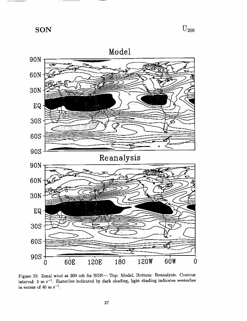
Figure 22: Zonal wind at 200 mb for SON-- Top: Model, Bottom: Reanalysis. Contourinterval: 5 m s -1. Easterlies indicated by dark shading, light shading indicates westerlies

in excess of 40 m s-1.

37

DJF Usso

90NModel

60N

30N

EQ

30S

60S

90S

90NReanalysis

60N

30N

EQ

30S

60S

90S0 60E 120E 180 120W 60W 0

Figure 23: Zonal wind at 850 mb for DJF-- Top: Model, Bottom: Reanalysis. Contourinterval: 3 m s -1. Easterlies are shaded.

38

JJA Uss0

90NModel

60N

30N

EQ

30S

60S

90S

90NReanalysis

60N

30N

EQ

30S

60S

90S0 60E 120E 180 120W 60W 0

Figure 24: Zonal wind at 850 mb for JJA-- Top: Model, Bottom: Reanalysis. Contourinterval: 3 m s -1. Easterlies are shaded.

39

MAM Usso

90NModel

60N

30N

EQ

30S

60S ........

90S

90NReanalysis

60N

30N

EQ

30S

60S

90S0 60E 120E 180 120W 60W 0

Figure 25: Zonal wind at 850 mb for MAM-- Top: Model, Bottom: Reanalysis. Contourinterval: 3 m s -1. Easterlies axe shaded.

4O

SON U850

90NModel

60N

30N

EQ

30S

60S

90S

90N

60N

30N

EQ

30S

60S

90S

Reanalysis

I I

0 60E 120E 180 120W 60W 0

Figure 26: Zonal wind at 850 mb for SON-- Top: Model, Bottom: Reanalysis. Contourinterval: 3 m s -1. Easterlies are shaded.

41

DJF SLP

90N

60N

30N

EQ

30S

60S

90S

Model

90NReanalysis

60N

30N

sq

30S

60S

90S0 60E 120E 180 120W 60W 0

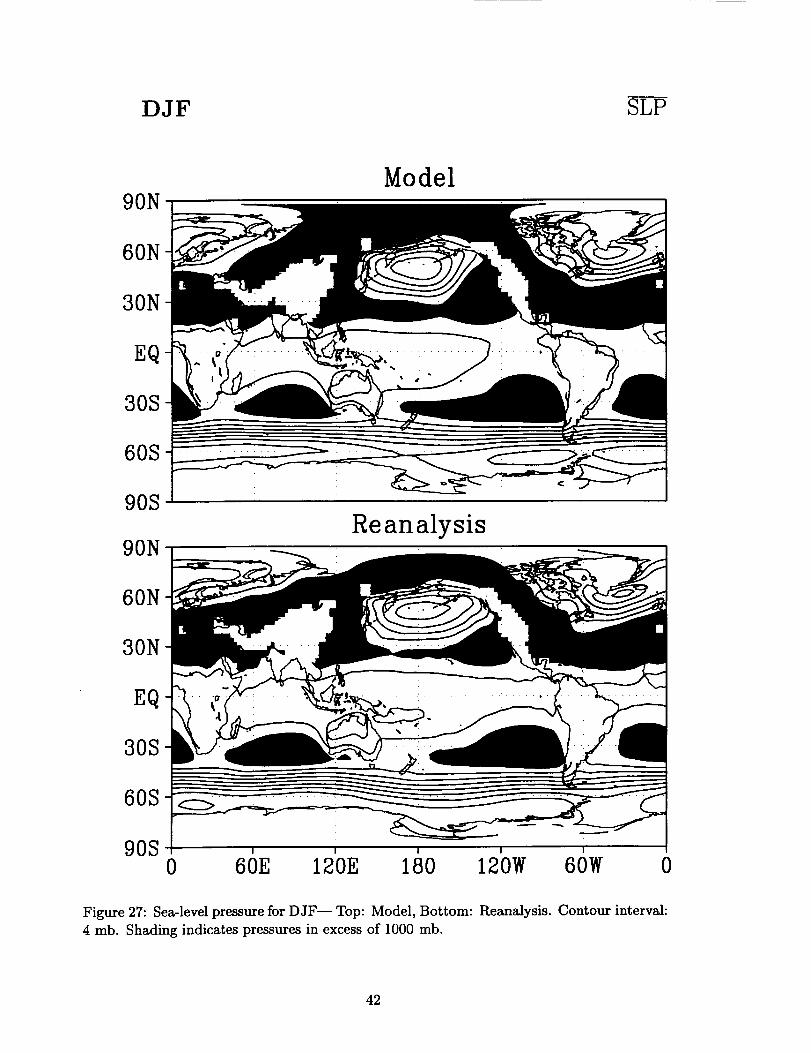
Figure 27: Sea-level pressure for DJF-- Top: Model, Bottom: Reanalysis. Contour interval:

4 mb. Shading indicates pressures in excess of 1000 mb.

42

JJA SLP

90NModel

60N

30N

EQ

30S

60S

90S

90NReanalysis

60N

30N

EQ

30S

60S

90S0 60E 120E 180 120W 60W 0

Figure 28: Sea-level pressure for JJA-- Top: Model, Bottom: Reanalysis. Contour interval:


43

MAM SLP

90NModel

60N

30N

EQ

30S

60S

90S

90NReanalysis

60N

30N

EQ

30S

60S

90S I I I I

0 60E 120E 180 120W 60W 0

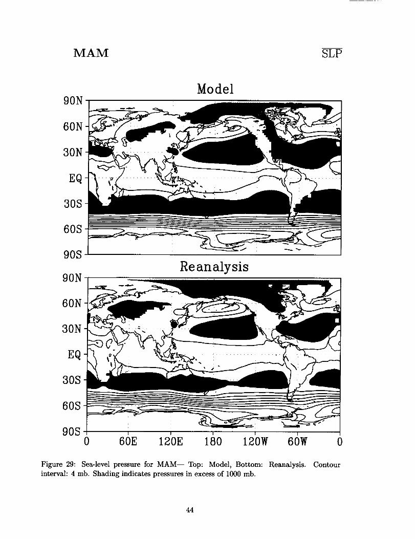
Figure 29: Sea-level pressure for MAM-- Top: Model, Bottom: Reanalysis. Contour

interval: 4 mb. Shading indicates pressures in excess of 1000 mb.

44

SON SLP

90N

60N

30N

EQ

30S

60S

90S

Model

90N

60N

30N

EQ

30S

60S

90S

Reanalysis

I I I I

0 60E 120E 180 120W 60W 0

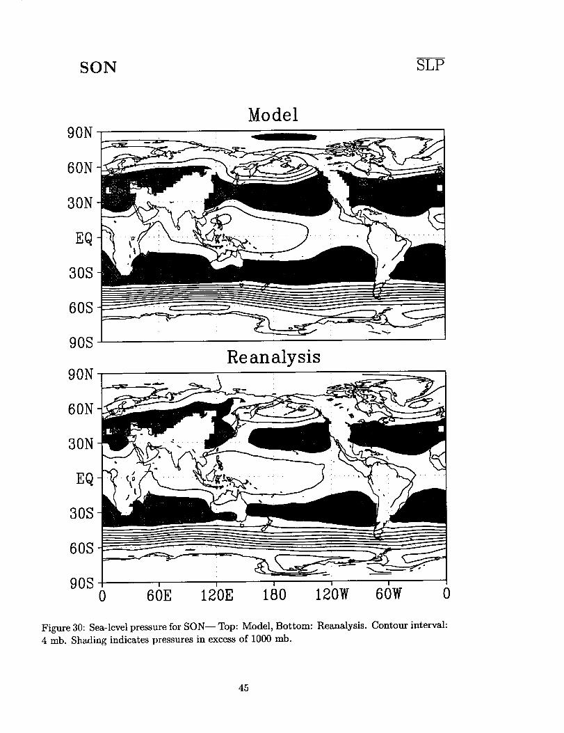
Figure 30: Sea-level pressure for SON-- Top: Model, Bottom: Reanalysis. Contour interval:


45

DJF Z*300

90NModel

60N

30N

EQ

30S

60S

90S

90NReanalysis

60N

30N

EQ

30S

60S

90S I ! I

0 60E 120E 180 120W 60W 0

Figure 31: Eddy geopotential height at 300 mb for DJF-- Top: Model, Bottom: Reanalysis.

Contour interval: 40 m. Shading indicates negative values.

46

JJA Z*3oo

90N

60N

30N

EQ

30S

60S

90S

Model

90NReanalysis

60N

30N

EQ

30S

60S

90S , , , ,0 60E 120E 180 120W 60W 0

Figure 32: Eddy geopotential height at 300 mb for JJA-- Top: Model, Bottom: Reanalysis.


47

MAM Z*3oo

90NModel

60N

30N

EQ

30S

60S

90S

90NReanalysis

60N

30N

EQ

30S

60S

90S I I I I I

0 60E 120E 180 120W 60W 0

Figure 33: Eddy geopotential height at 300 mb for MAM-- Top: Model, Bottom: Reanal-

ysis. Contour interval: 40 m. Shading indicates negative values.

48

SON Z*3oo

90N

60N

30N

EQ

30S

60S

90S

Model

90NReanalysis

60N

30N

EQ

30S

60S

90S _ , _0 60E 120E 180 120W 60W 0

Figure 34: Eddy geopotential height at 300 mb for SON-- Top: Model, Bottom: Reanalysis.


49

DJF _500

90NModel

60N

30N

EQ

30S

60S

90S

90NReanalysis

60N

30N

EQ

30S

60S

90S I I I I I

0 60E 120E 180 120W 60W 0

Figure 35: Omega at 500 mb (mb d-I) for DJF-- Top: Model, Bottom: Reanalysis.

Contour interval: 4 mb d -1. Shading indicates rising motion.

5O

JJA _500

90NModel

60N

30N

EQ

30S

60S

90S

90NReanalysis

60N

30N

EQ

30S

60S

90S I I I I I

0 60E 120E 180 120W 60W 0

Figure 36: Omega at 500 mb (mb d -1) for JJA-- Top: Model, Bottom: Reanalysis. Contour

interval: 4 mb d -1. Shading indicates rising motion.

51

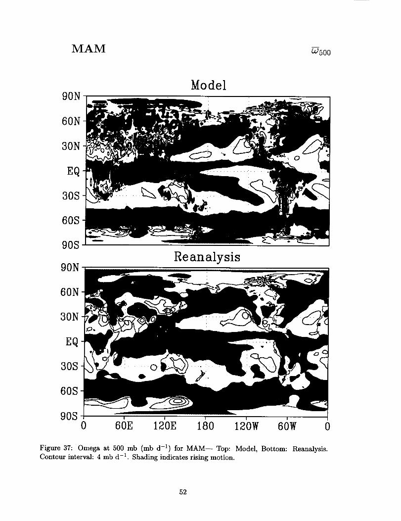
MAM _500

90NModel

60N

30N

EQ

30S

60S

90S

90NReanalysis

60N

30N

EQ

30S

60S

90S I I I I

0 60E 120E 180 120W 60W 0

Figure 37: Omega at 500 mb (rob d -i) for MAM-- Top: Model, Bottom: Reanalysis.

Contour interval: 4 mb d -1. Shading indicates rising motion.

52

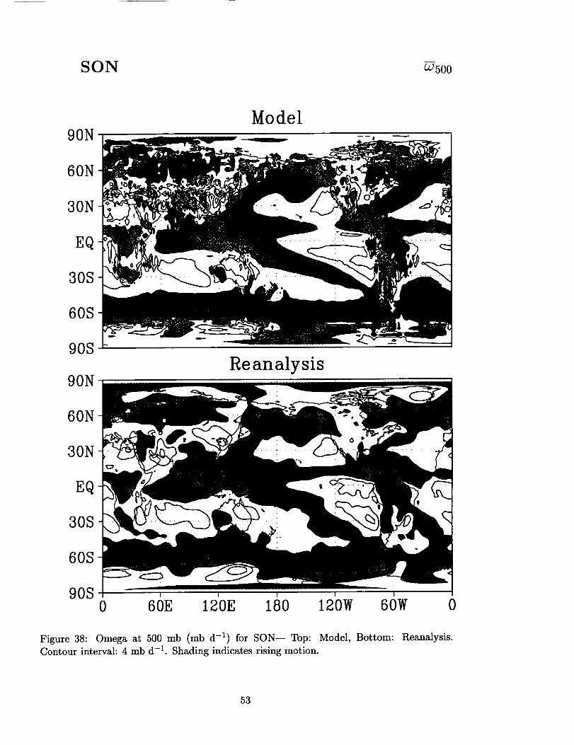
SON _5oo

90N

60N

30N

EQ

30S

60S

90S

90N

60N

30N

EQ

30S

60S

90S

Model

Reanalysis

I I I i I

0 60E 120E 180 120W 60W 0

Figure 38: Omega at 500 mb (mb d -1) for SON-- Top: Model, Bottom: Reanalysis.Contour interval: 4 mb d -1. Shading indicates rising motion.

53

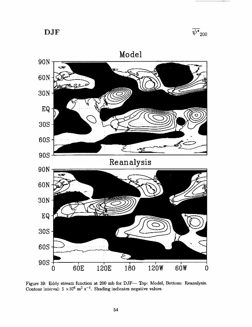
DJF ¢*9.00

90NModel

60N

30N

EQ

30S

60S

90S

90NReanalysis

60N

30N

EQ

30S

60S

90S ! !

0 60E 120E 180 120W 60W 0

Figure 39: Eddy stream function at 200 mb for DJF-- Top: Model, Bottom: Reanalysis.

Contour interval: 5 × 10 6 m 2 s -1. Shading indicates negative values.

54

JJA ¢*200

90NModel

60N

30N

EQ

30S

60S

90S

90NReanalysis

60N

30N

EQ

30S

60S

90S l I I

0 60E 120E 180 120W 60W 0

Figure 40: Eddy stream function at 200 mb for JJA-- Top: Model, Bottom: Reanalysis.

Contour interval: 5 ×10 6 m 2 s-1. Shading indicates negative values.

55

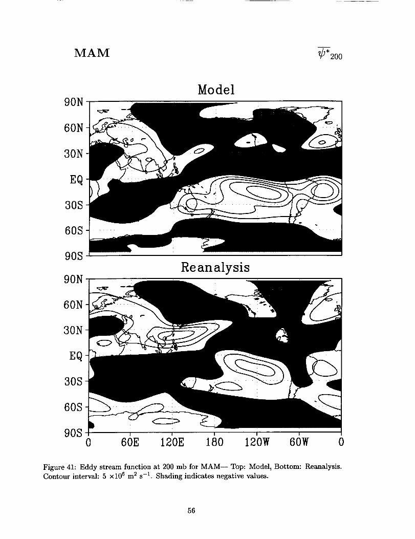
MAM ¢*200

90NModel

60N

30N

EQ

30S

60S

90S

90NReanalysis

60N

30N

EQ

30S

60S

90S I I I I I

0 60E 120E 180 120W 60W 0

Figure 41: Eddy stream function at 200 mb for MAM-- Top: Model, Bottom: Reanalysis.

Contour interval: 5 x 106 m 2 s -1. Shading indicates negative values.

56

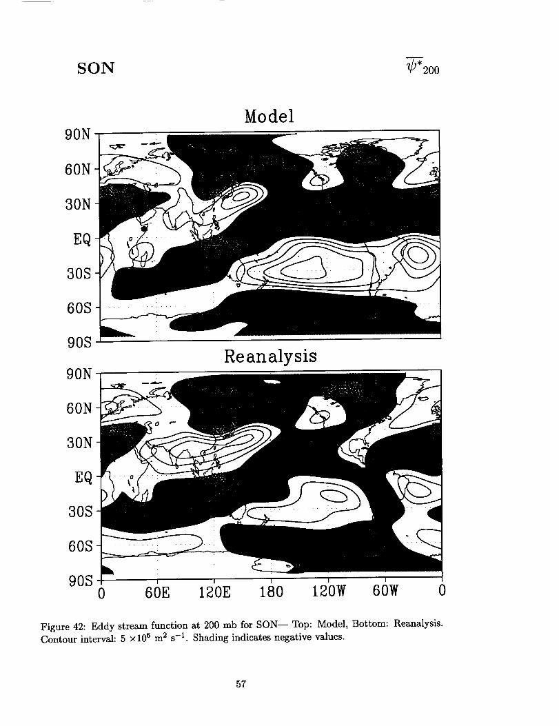
SON ¢'2oo

90NModel

60N

30N

Eq

30S

60S

90S

90NReanalysis

60N

30N

Eq

30S

60S

90S I I I

0 60E 120E 180 120W 60W 0

Figure 42: Eddy stream function at 200 mb for SON-- Top: Model, Bottom: Reanalysis.


57

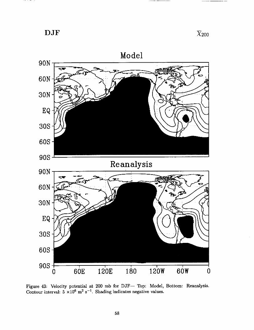
DJF X2oo

90N

60N

30N

EQ

30S

60S

90S

Model

90N

60N

30N

EQ

30S

60S

90S I I I

Reanalysis

0 60E 130E 180 120W 60W 0

Figure 43: Velocity potential at 200 mb for DJF-- Top: Model, Bottom: Reanalysis.

Contour interval: 5 x 106 m S s -1. Shading indicates negative values.

58

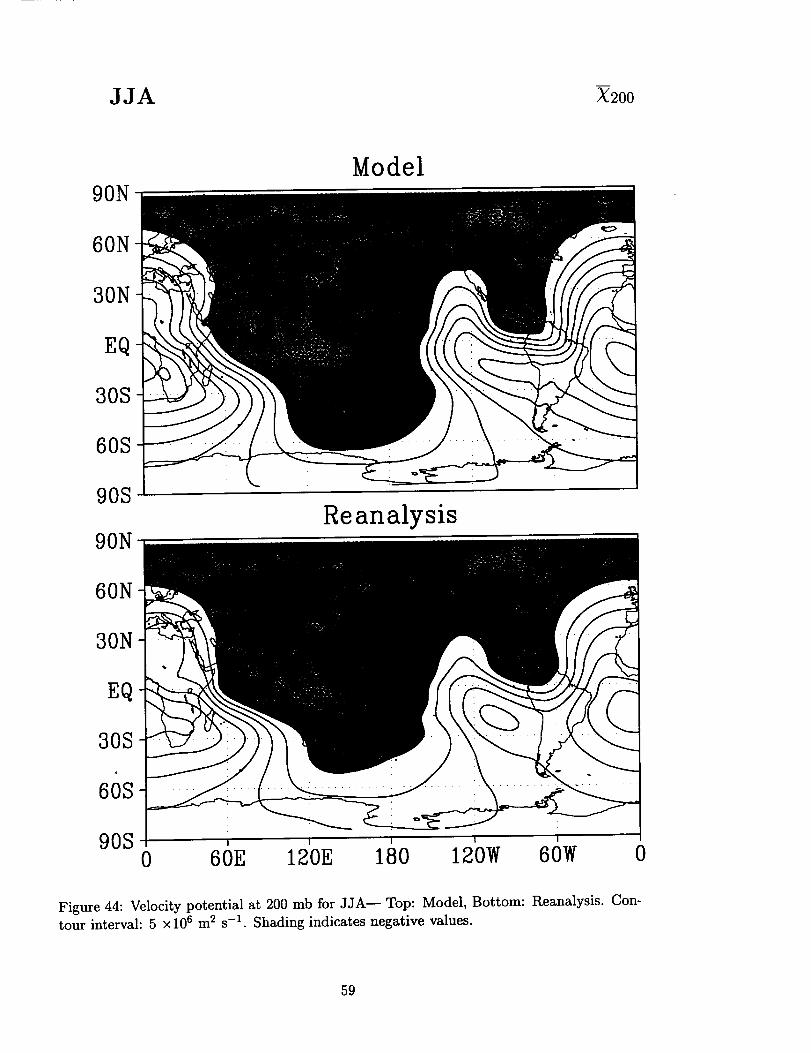
JJA X200

90NModel

60N

30N

EQ

30S

60S

90S

90NReanalysis

60N

30N

EQ

30S

60S

90S ! !

0 60E 120E 180 120W 60W 0

Figure 44: Velocity potential at 200 mb for JJA-- Top: Model, Bottom: Reanalysis. Con-

tour interval: 5 x 106 m 2 s -1. Shading indicates negative values.

59

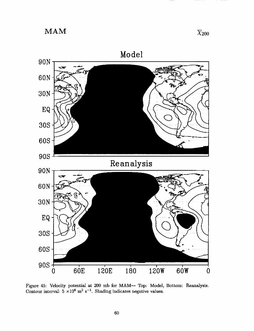
MAM X2oo

90NModel

60N

30N

EQ

30S

60S

90S

90NReanalysis

60N

3ON

EQ

30S

60S

90S i I I

0 60E 120E 180 120W 60W 0

Figure 45: Velocity potential at 200 mb for MAM-- Top: Model, Bottom: Reanalysis.


6O

SON _200

90NModel

60N

30N

EQ

30S

60S ......... -

90S

90NReanalysis

60N

30N

EQ

30S

60S ....... --

0 60E 120E 180 120W 60W 0

Figure 46: Velocity potential at 200 mb for SON-- Top: Model, Bottom: Reanalysis.

Contour interval: 5 xl06 m 2 s -1. Shading indicates negative values.

61

0

Q

0

o

o

0

o

0

62

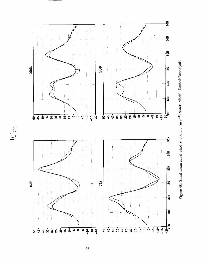
c'q

!0 _ 0 t_ 0 t_ 0 _ 0 U3 0 af3 0 _ 0u_ _P N" C"J C_ C_ C'_ --I ,,,..I I ',-_ --.q C_

I I I

Zo0_

.o

Z

r;3

_3

o

|1

Z

o_o_o_o_o_o_o_o °! I I

r_

c_

c_

c_

0

.,,-_

0

r_

c',,1

o ,,.._

c_

.,,._

63

oO

: i

I I I

Z

rD

i

9 I l

0

°_

/

Q_

°_

o_Q

gN

d_

°_,,i

64

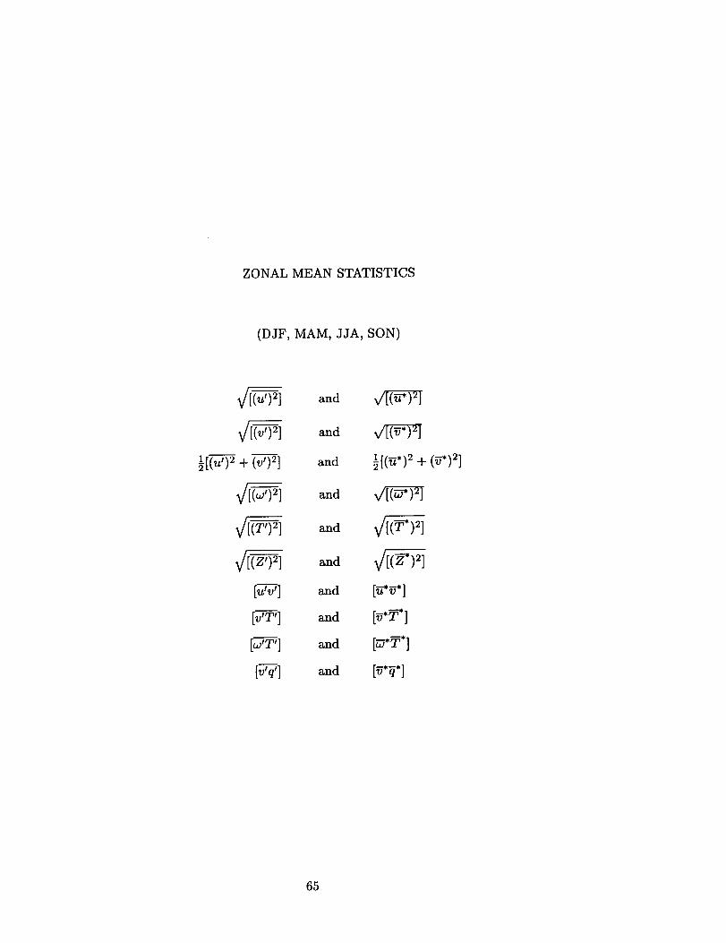
ZONAL MEAN STATISTICS


lr(u,)2_,. + (.,,,)2]

_/[(,,..,')':']

v_(T') 2]

v_(z') '_]

[_--_,]

[_-_T']

[,.,..,'T']

[_--_]

a,nd

and

and

and

and

and

and

and

and

and

1r(_*)2_,. + (_.)2]

V_(_) 2]

[_*_]

[_*_*]

[_*_*]

65

/

/

<

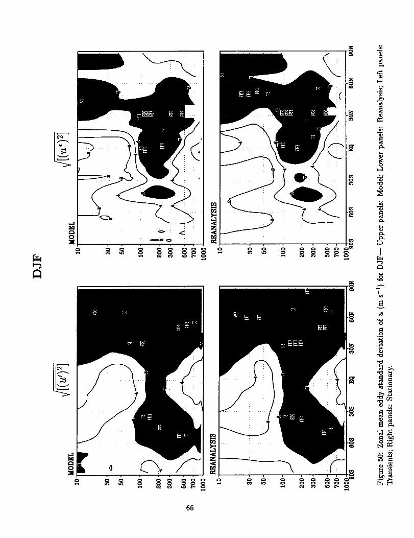
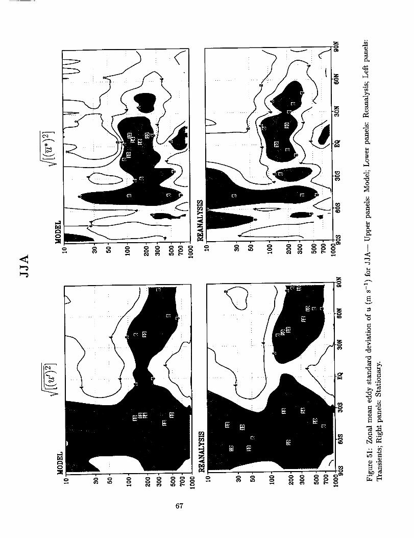
0 0

o_

0

<

I

v

o

0

o_

.o

67

0 0 0 0 0

o_

o

I

I

0

°_

o

68

Z©

69

0

o

I©

o

>

_0

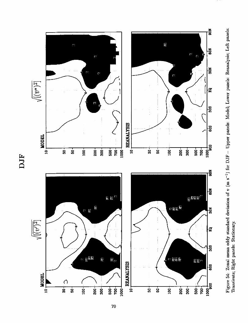
0i i 1 i i i !

0 0 0 0 0 0 0 0_ 0 0 0 0 0 0

! u i0 0 0

z

_ _ 0 0 0 0 0 0

o_

I

v

Q

0

o_

70

_J

o

o_

@

I<

_o

J

@

-o

U3

_J

71

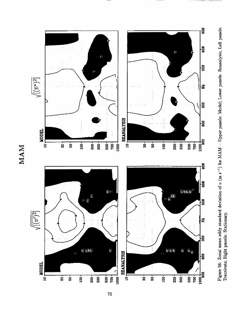
Z

.o

.o

Z.o

_3

c_

°_

o

I

I

v

O

o°_

Or_

_r_

_u0

o_

o_

72

Z©

! ! i J i

0 0 0 0 0 0

z

z

-0

0

0 0 0 _

0 0 0

0_

o

z©

I

o

°_

73

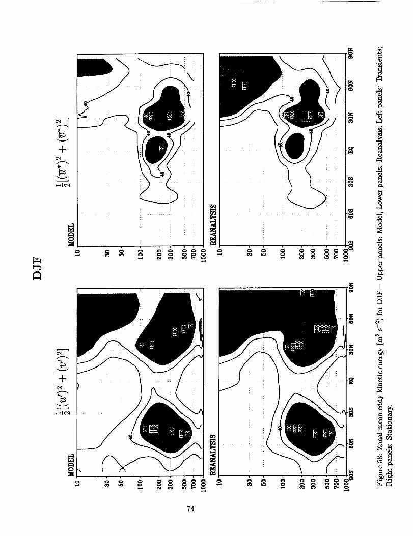
0

ov-4

i

oi i g | w

0 0 0 0 0 0 00 0 0 0 0 0

Z0

Z"0

Z"0

C/3

c_

c_

c_

c_

c_

o

O

c'q

°,,._

c_

74

\

/

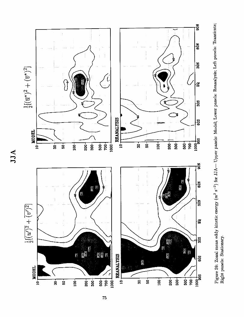
0

m i i

0 0 0LO 0

i i i |0 0 0 0 0 _

0 0 0 0 0

Z

o

-o

Z-0

o.

@

o

I_3

_q

o_ o_

?5

_o

o o _ _ _q.O

76

Z©

_Jc_

0

0

w w , ! i i i

0 0 0 0 0 0 0 0CO _'3 0 0 0 0 0 0

c__J

(_

_J

o

_J

_J

z©

I

_J

_J

77

00

00

78

00

c_

°_

o

I

I

o

o

°,-¢

cr_

_0°,-¢

<

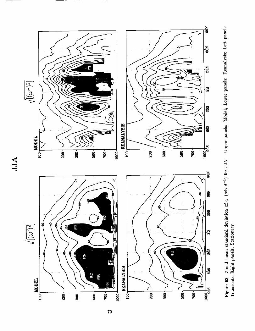
7g

00

00

o

o

c_

<

1

3

o

o°_

_o_r_

°_

o.

80

C/3

°_

o

I

I

0

o

b0o

°o

°_

©

o_

o

I©

1

3

o

oo_

°_

°o

81

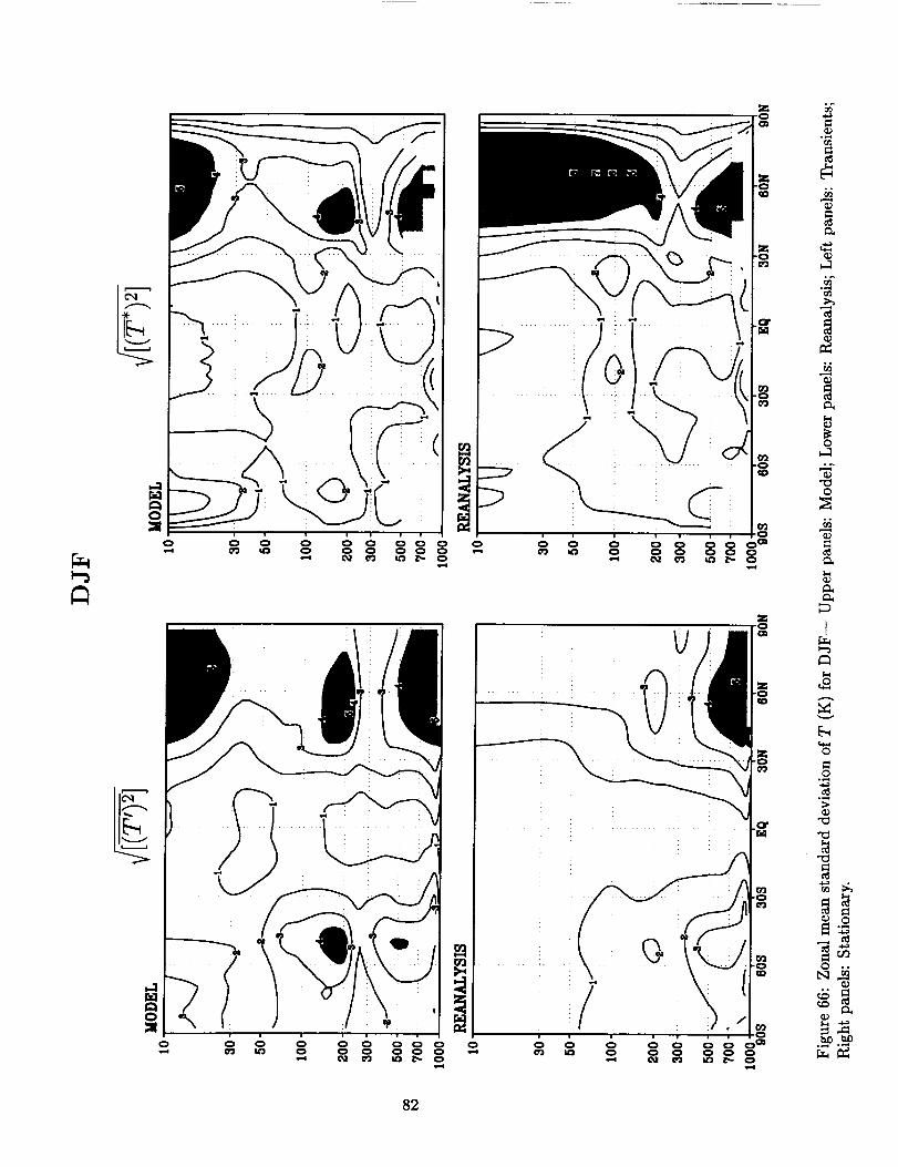
i ..... i

0 0 0 0 0 0 0 0 0_ _ 0 0 0 0 0 0

0 0 0

Q

0

O

o_

o

0

82

83

84

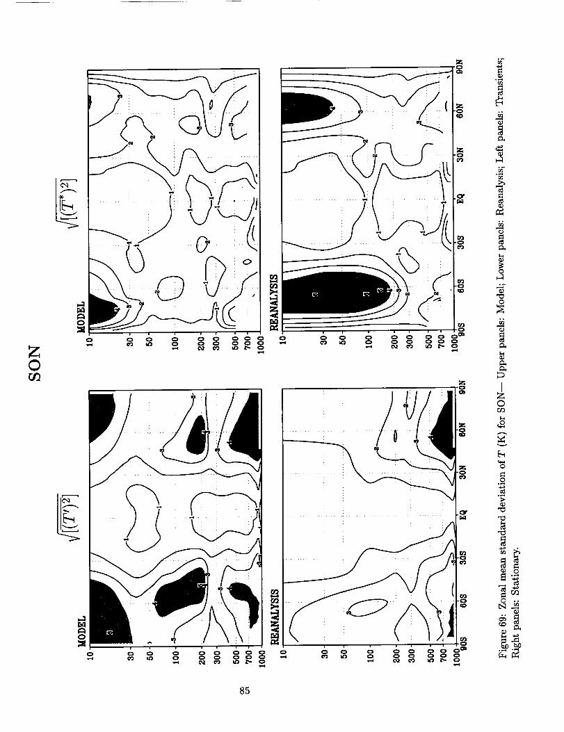
I=

q_

I=

°_

o

z©

v

E_

O

_p

o_._

o

A:I_0

85

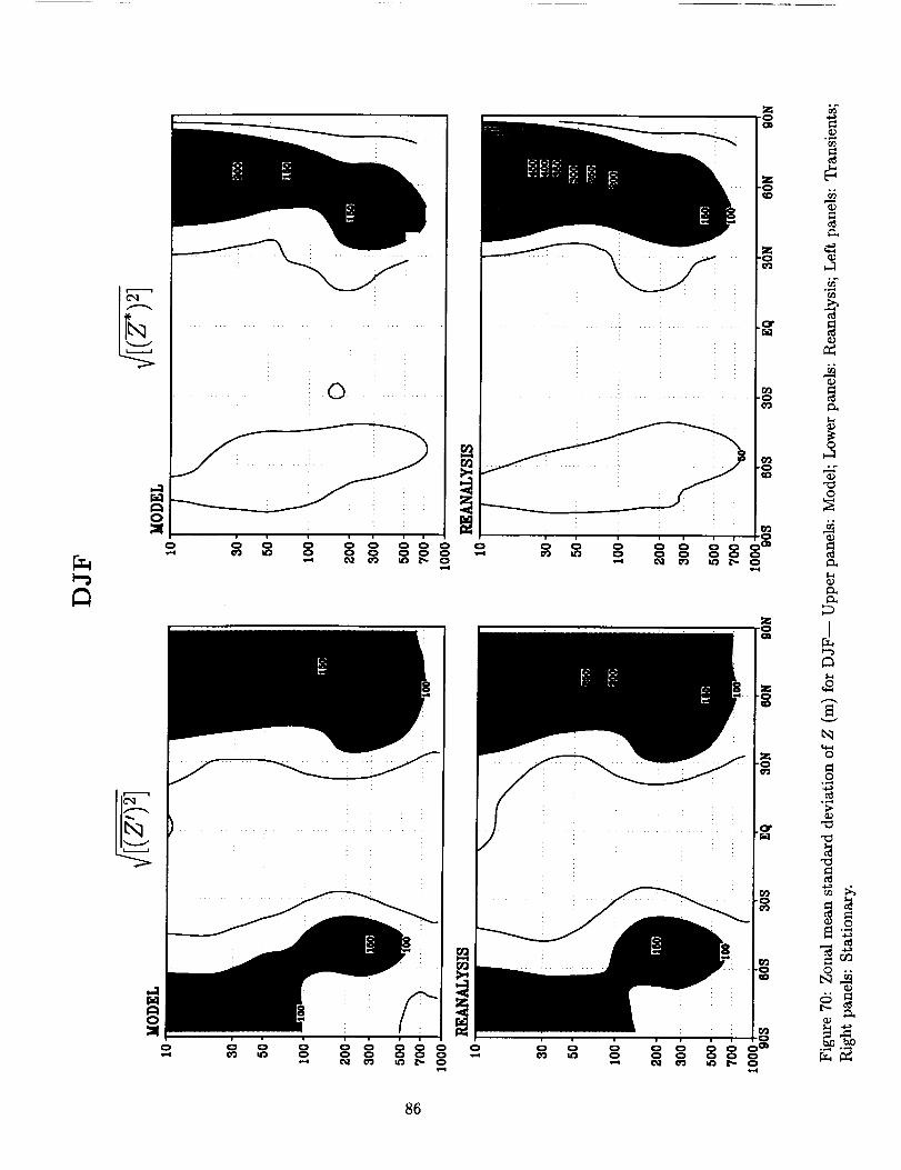
0

©

i i i | i i |0 0 0 0 0 0 0 0C_J _ 0 0 0 0 0 0

0

_D

C'3

............. _.......... 0C'3

03-0

z02

0

I

0

o_

0

86

<

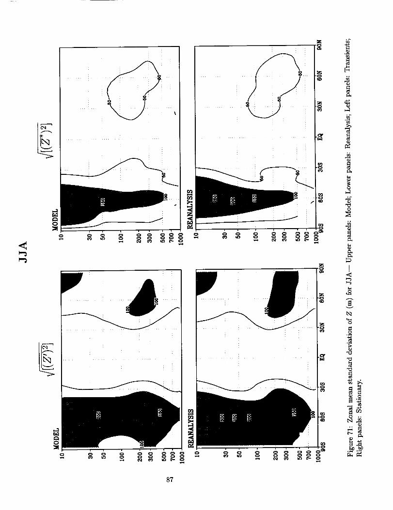
Z

ZCO

o_

o

0

oo_

o

87

\

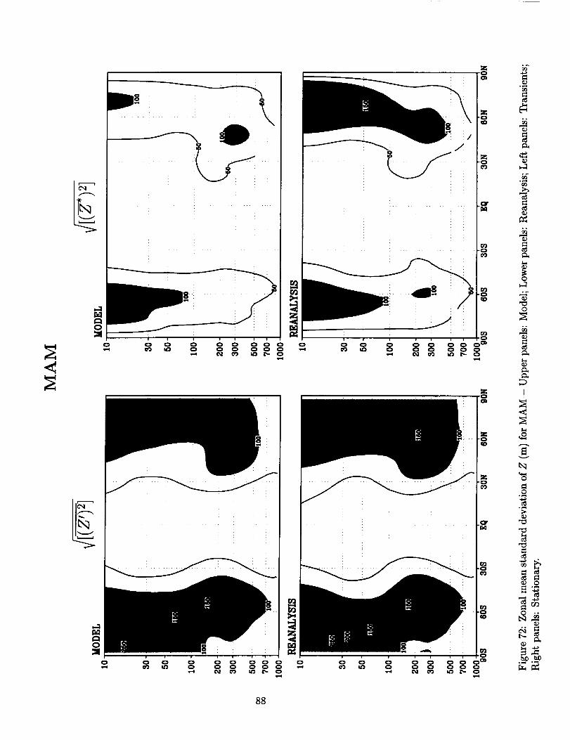
-0

o_

o

88

\

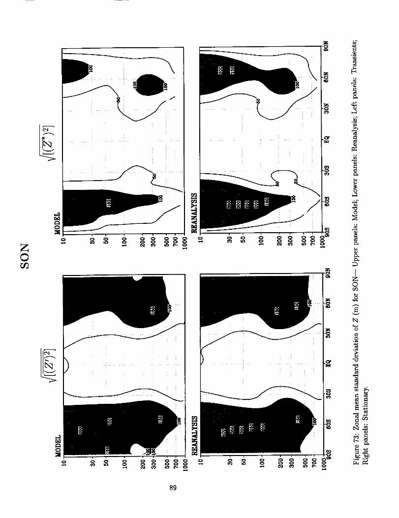
89

O'J

O'J

c_

.,-t

o

o

c_

©cf_

_o

o

.,..,

_ o

_D

90

zC_

qD

02

¢0

c_

o

I

J

c_

o

C/3

°_

Z

°_

O

I

I

0

oo

o_

91

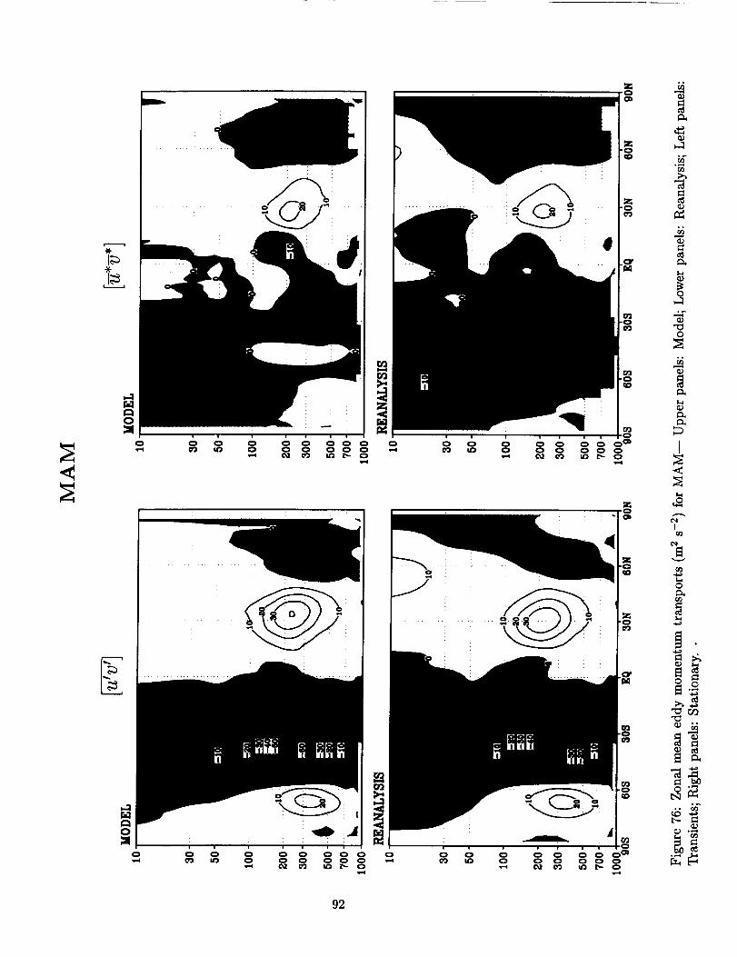
o o

Z

Z

Z

i i i i

"0

o_

o

I

I

0

°_

o_

0_

92

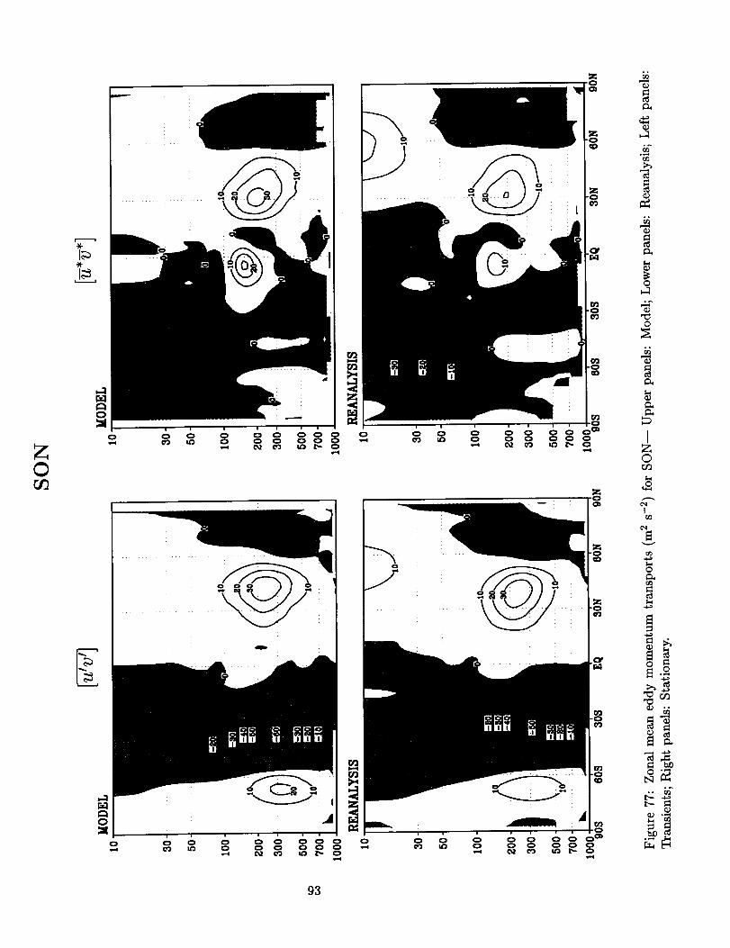
Z©

rJ3

0

c_

c_

o_

o

nz©

I_3

0

c_

°_

93

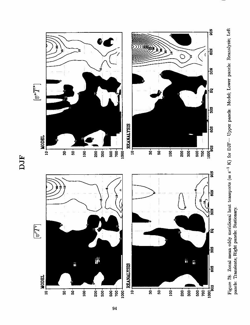
0

0 0 0 0 0 0 0 0 0_ 0 0 0 0 0 0

-0

-0

0 0 0 00 0 0 0 0

0_

0

I

94

<

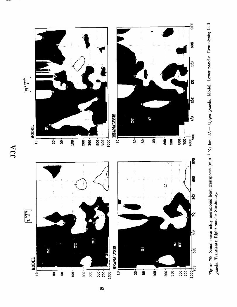
g5

z0O_

00

0

°_

0

I

C_3

0

o

b_°,_

o'_

L"-

• _

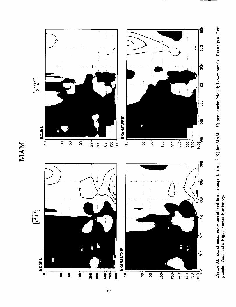
z"0

z

o_ _ o__i ° , .o o o oo °o oOoOoO o o o oo o °o oooo o_

o

J

173

0

O0_

O0

96

Z©

0

0

O2

0

c_

F_

0

I

©U_

7_3

0

o.,'_

oo,.._Nm

°_

g7

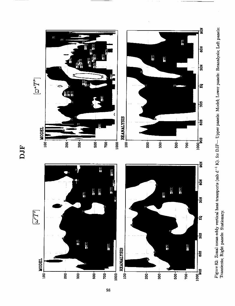
00

o_

2_

0

o_b_

98

.......... !

gg

000

0003

00

00

°_

0

I<

_3

0

_r_

O0

C_3

*

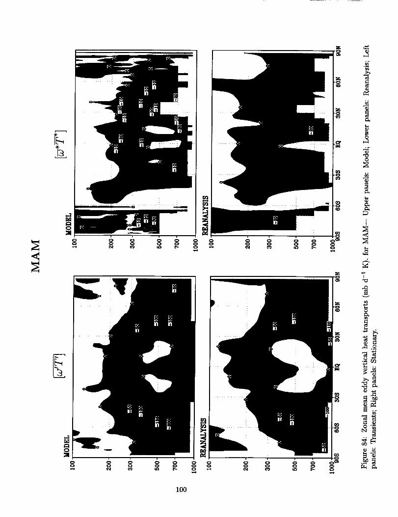
0o

00

100

00

00

°_

0

2_

I

0

.,.._

Z©

o 00 0

101

c_

c_

°_

o

c_

©rj_

o

°,_

_3

0"_L'q

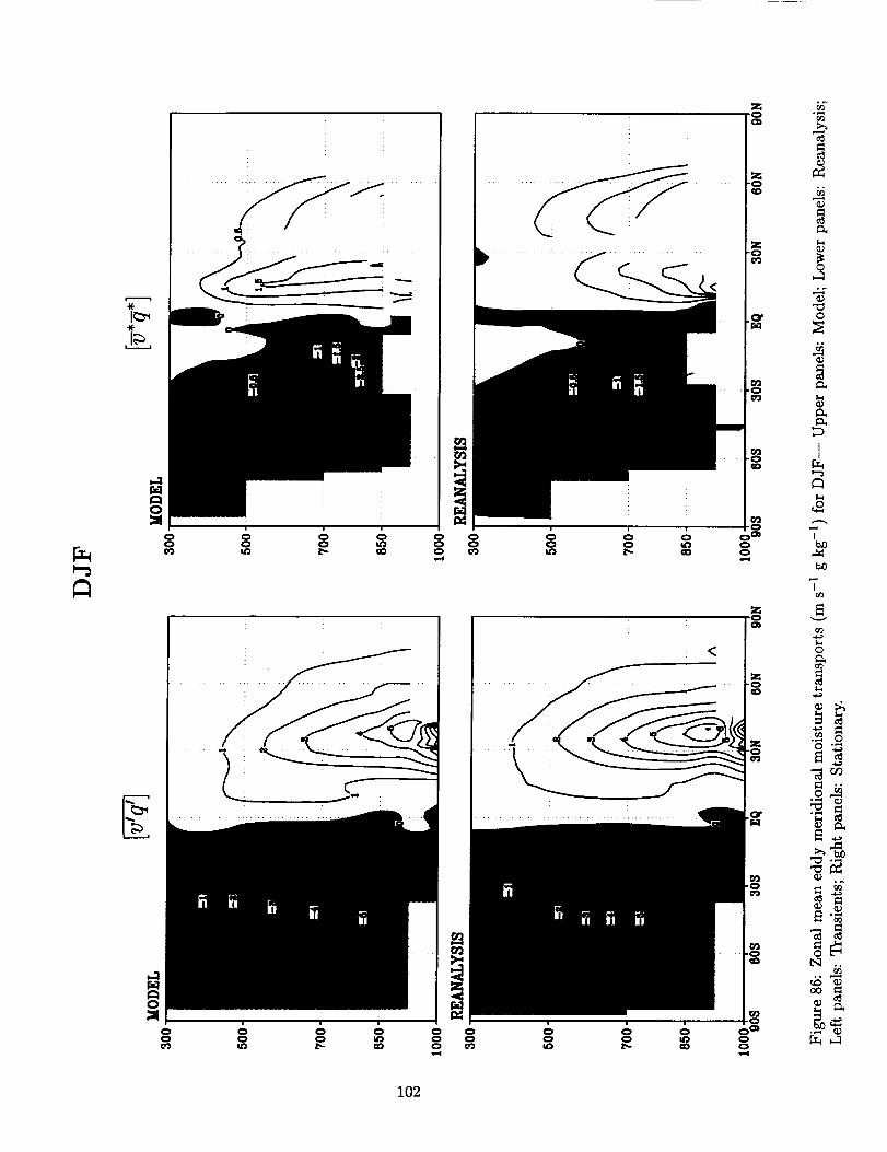
o

o

I

I

k_

°_

o_

o

o°

102

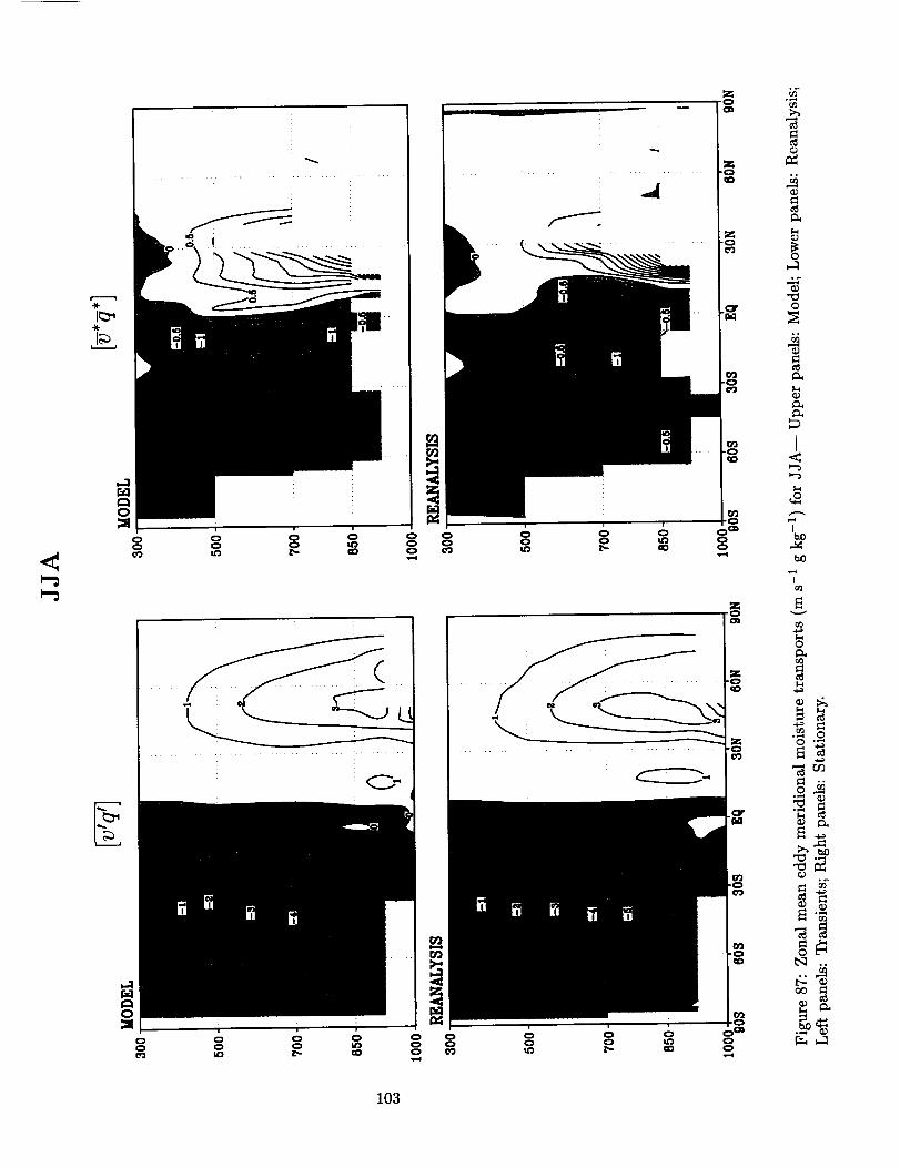
G-

.....___

oz

.zo

z

00

0

<

7

v

0

O ""_

_._

0

._N

103

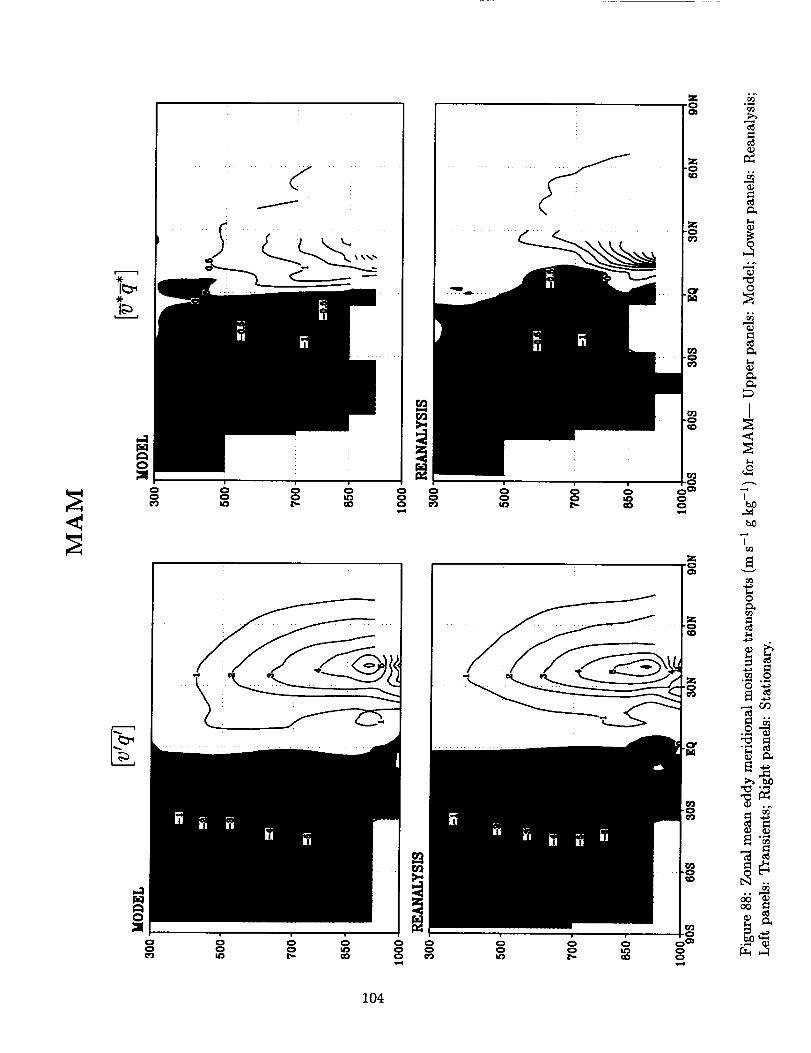
0

00

=

@

°_

@

I

I

o

o._

@

0°

104

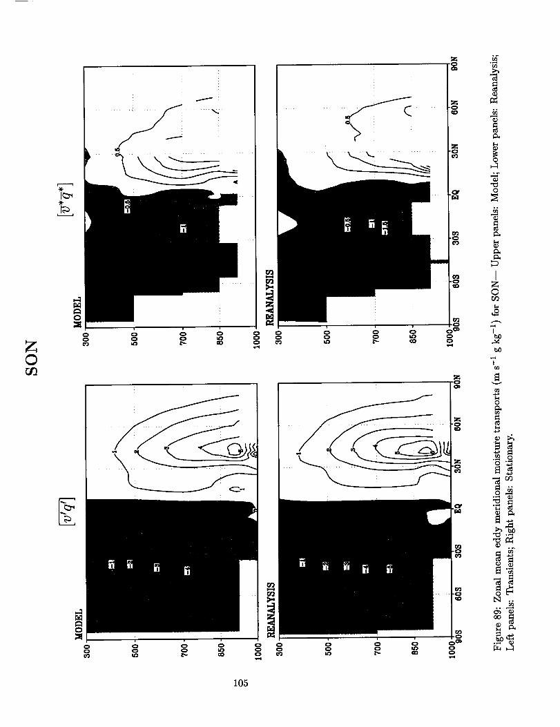
Z©

z

z

0 0 00 o u_

O_o0

p-4

°_

O

Iz©

0

Ct_

o_

..-_

Q;

0L_ o.

..

oo

105

+

/

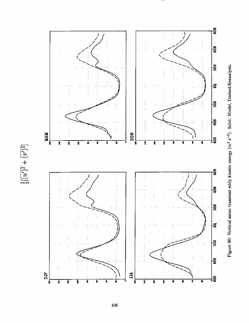
106

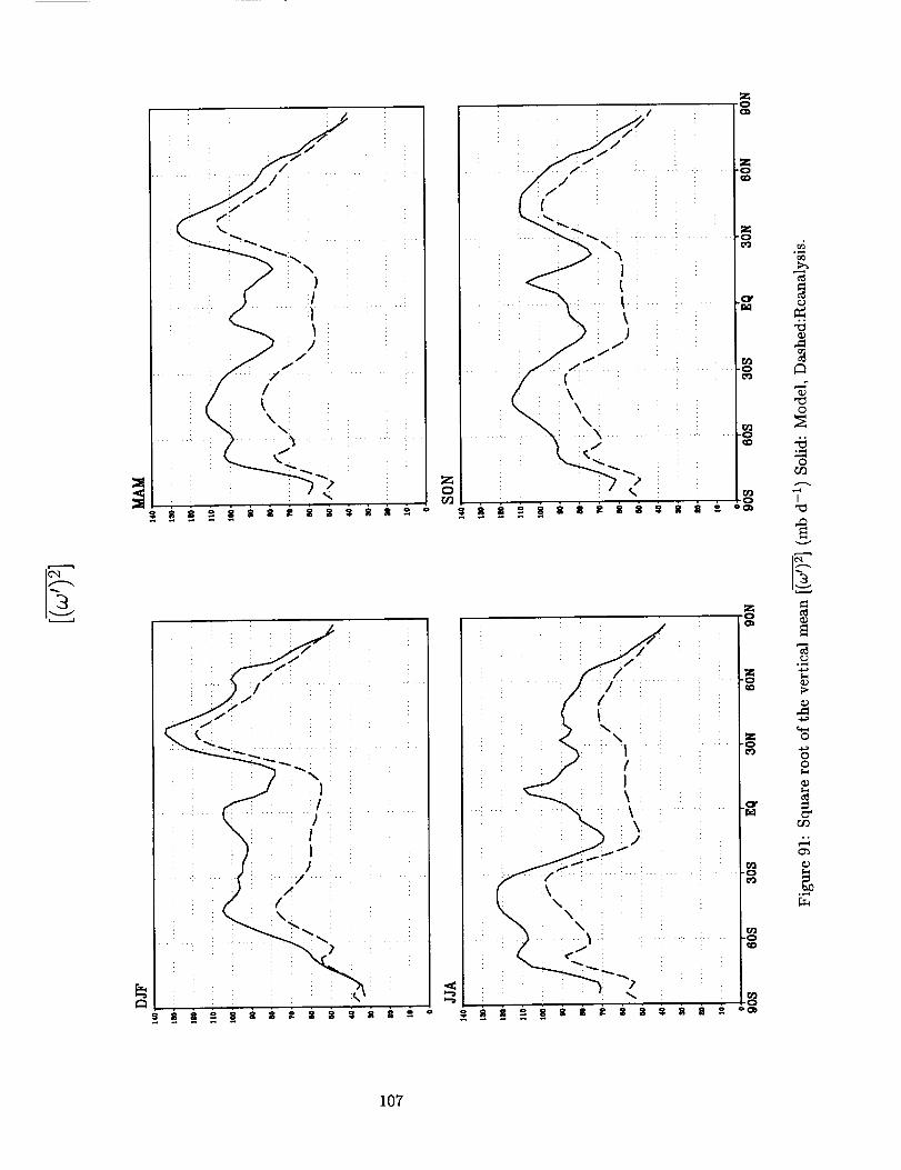
L

/

•i \1I

!

i iJ

\\ i.. .... ...

_ .

z

irJ'J

i i : i i !

: ii i :

i! .! i i ;/ i

O

o,.,_

o

I

_>

o

o@

°,._

107

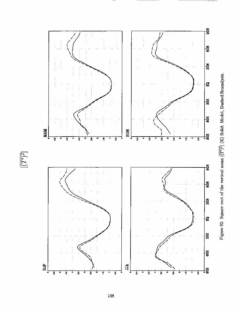
108

)/

//

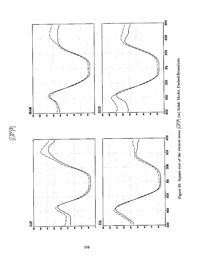
109

I\: i I

\\

!

110

i i i : :

Z

Z

Z-0

o

o

,Q,,;,

111

112

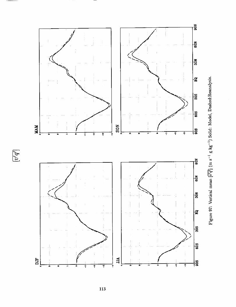
/ : _ i

z i i

_j

z

-0¢0

C_

¢t3

,..-,

0

°...q

0

J

b_3

°.-,

113

114

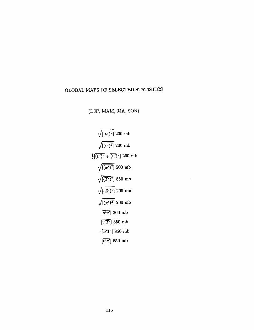
GLOBAL MAPSOF SELECTED STATISTICS


_200 mb

_200 mb

½t_-_+ _PJ 200_b

_500 mb

_850 mb

_200 nab

_200 mb

f_-_'J200_b

[v--Z_T_l850 mb

-t_-_T'J850_b

t.--_Jsso _b

115

DJF

90N

60N

30N

nq

30S

60S

90S

Model

90N

60N

30N

EQ

30S

60S

90S

Reanalysis

0 60E 120E 180 120W 60W 0

Figure 98: _[_7_] at 200rob for DJF-- Top: Model, Bottom: Reanalysis. Contour interval:

2 m s -1. Shading indicates values exceeding 6 m s -1.

116

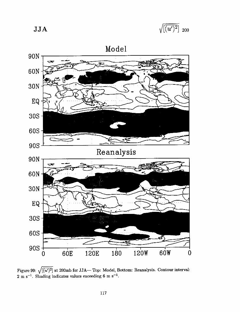
JJA :] :oo

90N

60N

30N

EQ

30S

60S

90S

Model

90N

60N

30N

EQ

30S

60S

90S

Reanalysis

0 60E 120E 180 120W 60W 0

Figure 99: _ at 200mb for JJA-- Top: Model, Bottom: Reanalysis. Contour interval:

2 m s-1. Shading indicates values exceeding 6 m s-1.

117

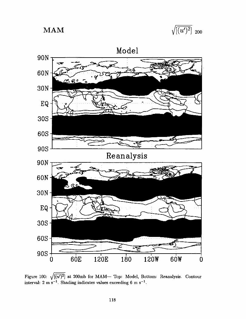
MAM 20o

90NModel

60N

30N

EQ

30S

60S

90S

Reanalysis90N

60N

30N

EQ

30S

60S

90S I i I I I

0 60E 130E 180 120W 60W 0

F_- _

Figure 100: _/[(u') 2] at 200mb for MAM-- Top: Model, Bottom: Reanalysis. Contour

interval: 2 m s -1. Shading indicates values exceeding 6 m s -1.

118

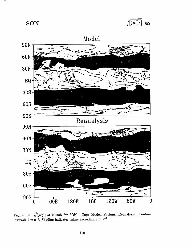
SON

90NModel

60N

30N

EQ

30S

60S

90S

90NReanalysis

60N

30N

EQ

30S

60S

90S0 60E 120E 180 120W 60W 0

Figure 101: _/[(u') _] at 200mb for SON-- Top: Model, Bottom: Reanalysis. Contour

interval: 2 m s-1. Shading indicates values exceeding 6 m s -1.

119

DJF

90NModel

60N

30N

EQ

30S

60S

90S

90NReanalysis

60N

30N

EQ

30S

60S

90S0 60E 120E 180 120W 60W 0

Figure 102: _ at 200rob for DJF-- Top: Model, Bottom: Reanalysis. Contour


120

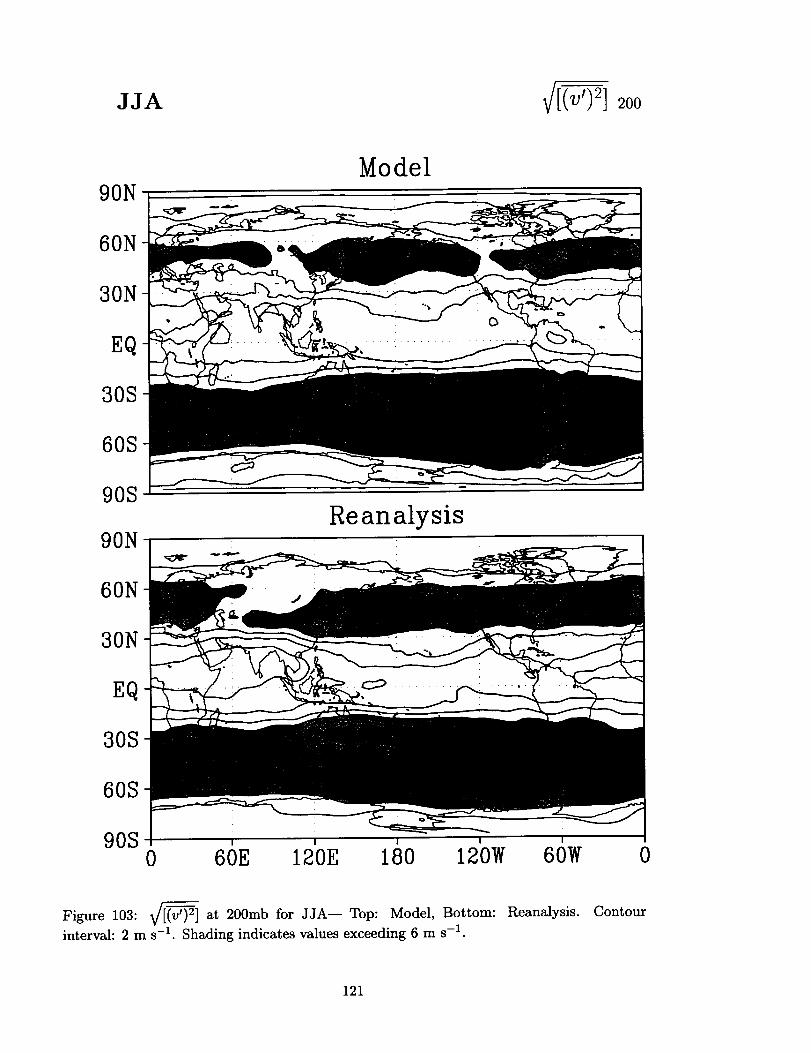
JJA

90N

Model

60N

3ON

EQ

30S

60S

90S

90N

60N

30N

EQ

30S

60S

90S

Reanalysis

I I I I

0 60E 120E 180 120W 60W 0

Figure 103: y_v') 2] at 200mb for JJA-- Top: Model, Bottom: Reanalysis. Contour


121

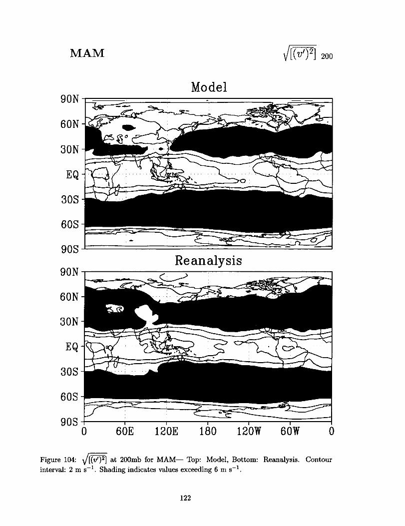
MAM 2o0

90NModel

60N

30N

EQ

30S

60S

90S

90N

60N

30N

EQ

30S

60S

90S

Reanalysis

! !

0 60E 130E 180 120W 60W 0

Figure 104: _/[(v') 2] at 200mb for MAM-- Top: Model, Bottom: Reanalysis. Contour


122

SON :oo

90NModel

60N

30N

EQ

30S

60S

90S

Reanalysis90N

60N

30N

EQ

30S

60S

90S ! I

0 60E 120E 180 120W 60W 0

Figure 105: y/_v') 2] at 200rob for SON-- Top: Model, Bottom: Reanalysis. Contour


123

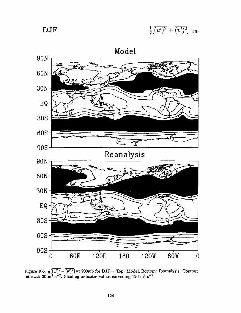
DJF ½[(_'):+ (v')_]_00

90NModel

60N

30N

EQ

30S

60S

90S

90NReanalysis

60N

30N

EQ

30S

60S

90S I

0 60E 120E 180 120W 60W 0

Figure 106: ½[(u') 2 + (v') 2] at 200rob for DJF-- Top: Model, Bottom: Reanalysis. Contour

interval: 30 m 2 s -2. Shading indicates values exceeding 120 m 2 s -2.

124

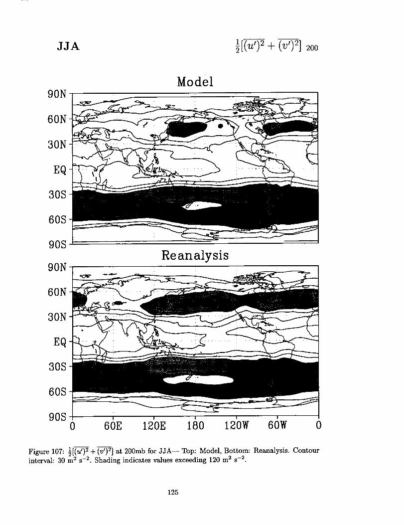
JJA 200

90NModel

60N

30N

EQ

30S

60S

90S

90N

60N

30N

EQ

30S

60S

90S

Reanalysis

I !

0 60E 120E 180 120W 60W 0

Figure 107: ½[(u') 2 + (v') 2] at 200mb for JJA-- Top: Model, Bottom: Reanalysis. Contourinterval: 30 m 2 s-2. Shading indicates values exceeding 120 m 2 s -2.

125

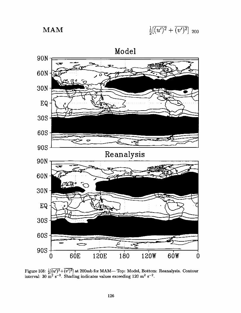
MAM 1 i 2 200) +

90NModel

60N

30N

EQ

30S

60S

90S

Reanalysis90N

60N

30N

EQ

30S

60S ........

90S , , ,0 60E 120E 180 120W 60W 0

1 t2 _t2Figure 108: _[(u ) + ( ) ] at 200mb for MAM-- Top: Model, Bottom: Reanalysis. Contourinterval: 30 m 2 s-2. Shading indicates values exceeding 120 m 2 s-2.

126

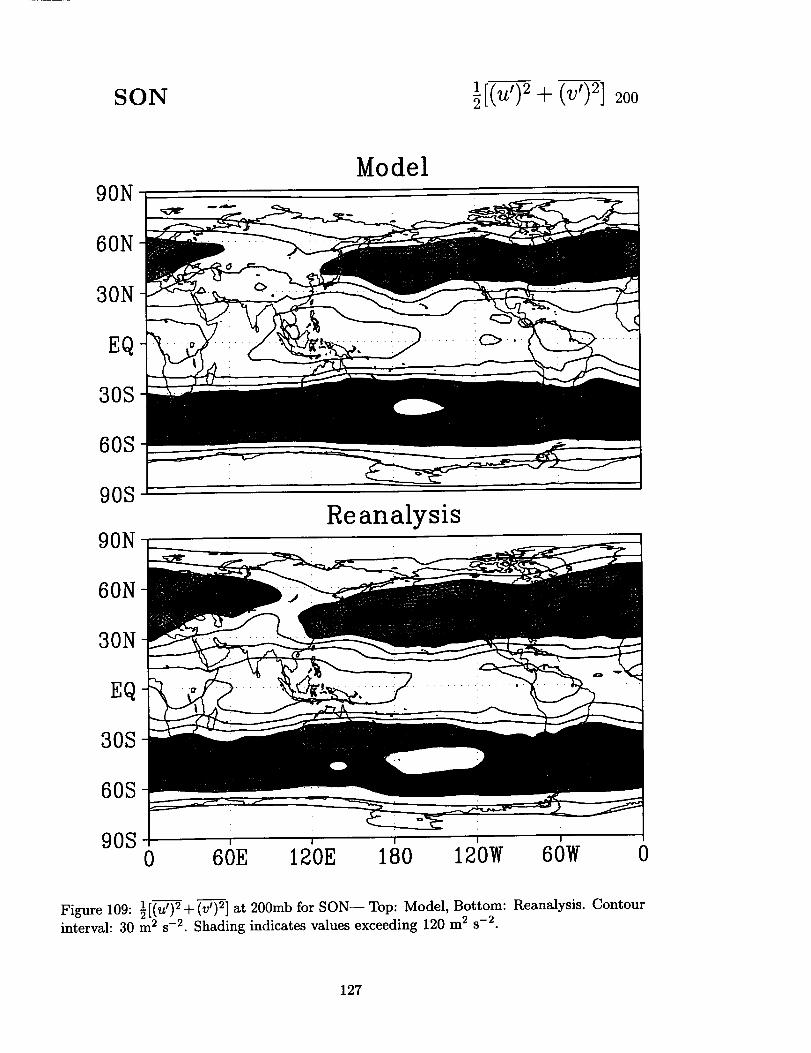
SON _r_u'):+ (v'):] _ooLk

90NModel

60N

30N

EQ

30S

60S

90S

90NReanalysis

60N

30N

EQ

30S

60S

90S !

0 60E 120E 180 120W 60W 0

Figure 109:1[(u')2 ÷ (v') 2] at 200mb for SON-- Top: Model, Bottom: Reanalysis. Contour

interval: 30 m 2 s -2. Shading indicates values exceeding 120 m 2 s -2.

127

DJF

90NModel

60N

30N

EQ

30S

60S

90S

90NReanalysis

60N

30N

EQ

30S

60S

90S I I I

0 60E 120E 180 120W 60W 0

Figure 110: _/[(w') 2] at 500mb for DJF-- Top: Model, Bottom: Reanalysis. Contour

interval: 20 mb d -1. Shading indicates values exceeding 120 mb d -1.

128

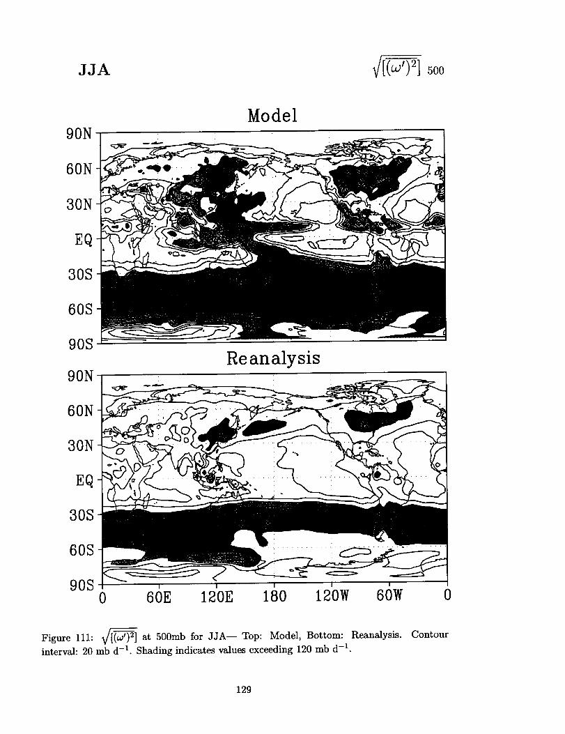
JJA

90NModel

60N

30N

EQ

30S

60S

90S

90NReanalysis

60N

30N

EQ

30S

60S

90S I I I I I

0 60E 120E 180 120W 60W 0

F_ _

Figure 111: _/[(w') 2] at 500mb for JJA-- Top: Model, Bottom: Reanalysis. Contour


129

MAM 500

90NModel

60N

30N

EQ

30S

60S

90S

90NReanalysis

60N

30N

EQ

30S

60S

90S0 60E 120E 180 120W 60W 0

Figure 112: ¢[(w') 2] at 500rob for MAM-- Top: Model, Bottom: Reanalysis. Contour


130

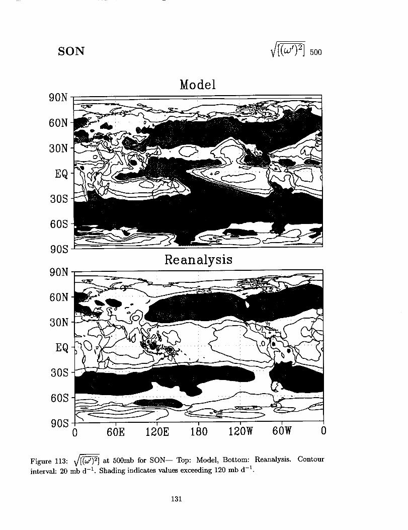
SON

90NModel

60N

30N

EQ

30S

60S

90S

90NReanalysis

60N

30N

EQ

30S

60S

90S , ,0 60E 120E

I

180 120W 60W 0

Figure 113: 9/[(w')2] at 500mb for SON-- Top: Model, Bottom: Reanalysis. Contour


131

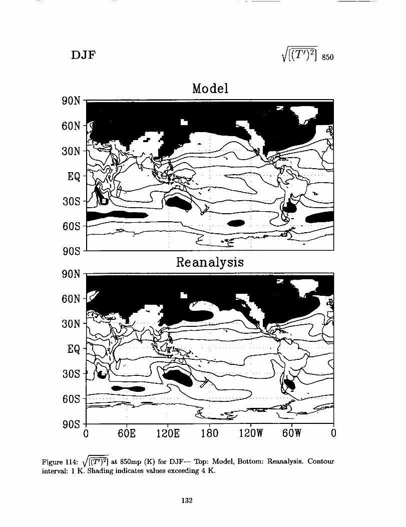
DJF ([_-_ 2] sso

90NModel

60N

30N

EQ

30S

60S

90S

90NReanalysis

60N

30N

EQ

30S

60S

90S0 60E 120E 180 120W 60W 0

f

Figure 114: _/[(T') 2] at 850mp (K) for DJF-- Top: Model, Bottom: Reanalysis. Contour

interval: 1 K. Shading indicates values exceeding 4 K.

132

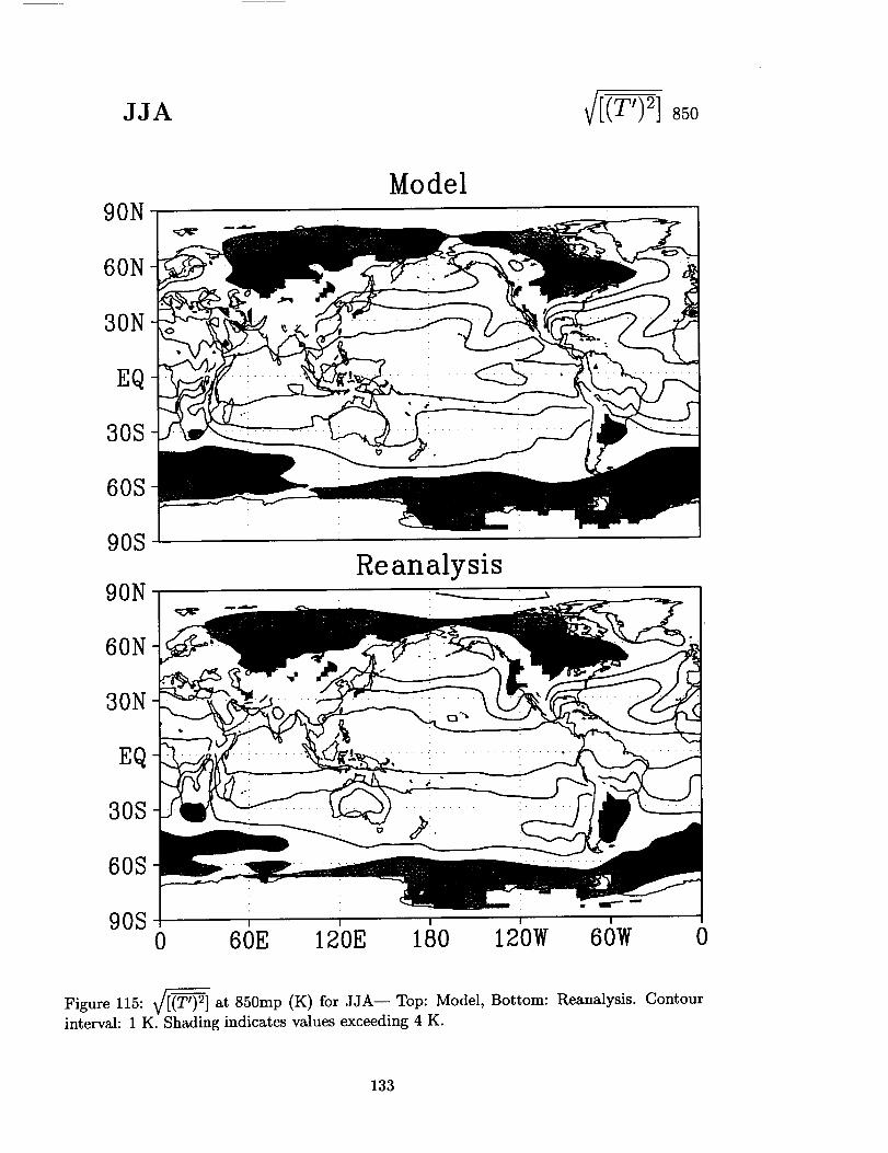
JJA

90N

60N

30N

EQ

30S

60S

90S

Model

90NReanalysis

60N ':

30N

EQ

30S

60S

90S0 60E 120E 180 120W 60W 0

Figure 115: _/_(T') 2] at 850mp (K) for JJA-- Top: Model, Bottom: Reanalysis. Contour


133

MAM

90NModel

60N

30N

EQ

30S

60S

90S

90NReanalysis

60N

30N

EQ

30S

60S

90S0 60E 120E 180 120W 60W 0

Figure 116: _[(T') 2] at 850mp (K) for MAM-- Top: Model, Bottom: Reanalysis. Contourinterval: 1 K. Shading indicates values exceeding 4 K.

134

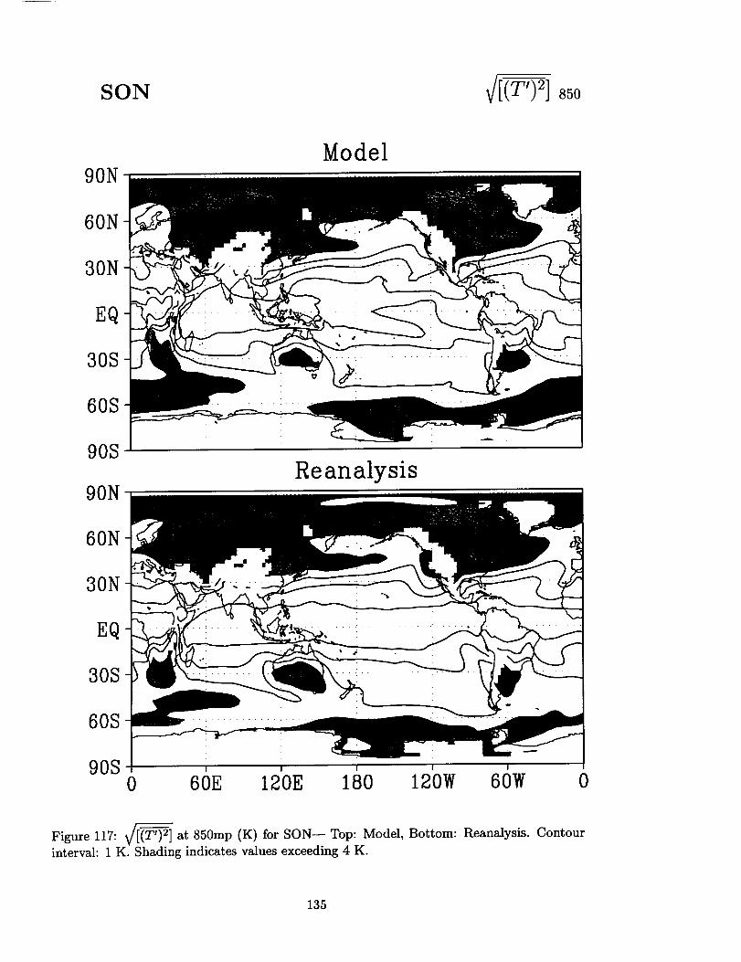
SON _/[(T') 2] 85o

90NModel

60N

30N

EQ

30S

60S

90S

90N

60N

30N

EQ

30S

60S

90S

Reanalysis

0 60E 120E 180 120W 60W 0

Figure 117: V/_(T') 2] at 850rap (K) for SON-- Top: Model, Bottom: Reanalysis. Contour


135

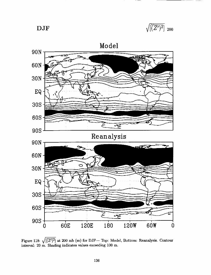
DJF _/[_)-2] 2oo

90N

60N

30N

EQ

30S

60S

90S

Model

90NReanalysis

60N

30N

EQ

30S

60S ........

90S0 60E 120E 180 120W 60W 0

/-

Figure 118: _/[(Z') 2] at 200 mb (m) for DJF-- Top: Model, Bottom: Reanalysis. Contour

interval: 20 m. Shading indicates values exceeding 100 m.

136

JJA

90NModel

60N

30N

EQ

30S

60S

90S

90NReanalysis

60N

30N

EQ

30S

60S

90S0 60E 120E 180 120W 60W 0

Figure 119: _/[(Z') 2] at 200 mb (m) for JJA-- Top: Model, Bottom: Reanalysis. Contour


137

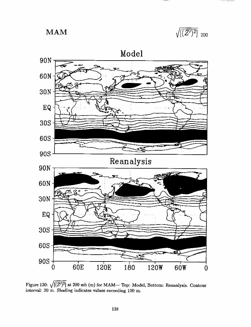
MAM 20o

90NModel

60N

30N

EQ

30S

60S

90S

90NReanalysis

60N

30N

EQ

30S

60S

90S I I I I

0 60E 120E 180 120W 60W 0

Figure 120: ¢[(Z') 2] at 200 mb (m) for MAM-- Top: Model, Bottom: Reanalysis. Contour


138

SON

90NModel

60N

3ON

EQ

30S

60S

90S

90NReanalysis

60N

30N

EQ

30S

60S

90S0 60E 120E 180 120W 60W 0

f=.

Figure 121: _/[(Z_) 2] at 200 mb (m) for SON-- Top: Model, Bottom: Reanalysis. Contourinterval: 20 m. Shading indicates values exceeding 100 m.

139

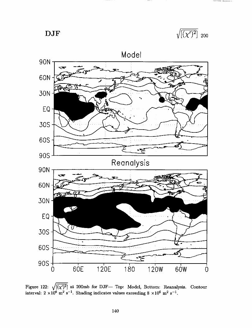
DJF

90NModel

60N

30N

EQ

30S

60S

90S

90NReanalysis

60N

30N

EQ

30S

60S ...........................

90S , , ,0 60E 120E 180 120W 60W 0

Figure 122: .V/[(XO2] at 200mb for DJF-- Top: Model, Bottom: Reanalysis. Contour

interval: 2 × 106 m 2 s-1. Shading indicates values exceeding 8 × 106 m 2 s -1.

140

JJA :oo

90NModel

60N

30N

EQ

30S

60S

90S

90NReanalysis

60N

30N

EQ

30S

60S

90S I

0 60E 120E 180 120W 60W 0

F

Figure 123: VI[(X') 2] at 200mb for JJA-- Top: Model, Bottom: Reanalysis. Contour

interval: 2 x 106 m 2 s-1. Shading indicates values exceeding 8 x 106 m 2 s -1.

141

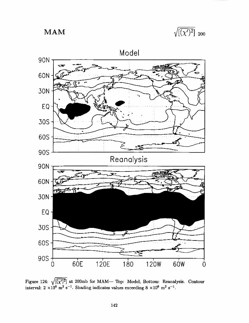
MAM 2oo

90NModel

60N

30N

EQ

30S

60S

90S

90NReanalysis

60N

3ON

EQ

30S

60S

90S0 60E 120E 180 120W 60W 0

Figure 124: _ at 200mb for MAM-- Top: Model, Bottom: Reanalysis. Contour

interval: 2 xl06 m 2 s -1. Shading indicates values exceeding 8 ×106 m 2 s -1.

142

SON

90N

60N

3ON

EQ

30S

60S

90S

Model

90NReanalysis

60N

30N

EQ

0 60E 120E 180 120W 60W 0

Figure 125: V/_X_) 2] at 200rob for SON-- Top: Model, Bottom: Reanalysis. Contour

interval: 2 x 106 m 2 s -1. Shading indicates values exceeding 8 x 106 m 2 s -1.

143

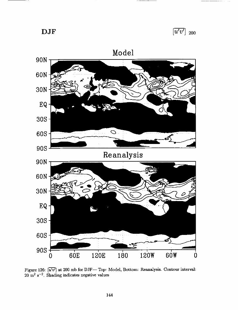
DJF _ 200

90NModel

60N

30N

EQ

30S

60S ..................... : .... _ '

90S

90N

60N

30N

EQ

30S

60S

90S

Reanalysis

I I I

0 60E 120E 180 120W 60W 0

Figure 126: [u-%Tv_] at 200 mb for DJF-- Top: Model, Bottom: Reanalysis. Contour interval:

20 m s s -2. Shading indicates negative values

144

JJA [_ 200

90N

60N

30N

EQ

30S

60S

90S

Model

90NReanalysis

60N

30N

EQ

30S

60S

90S , , , , '0 60E 120E 180 120W 60W 0

Figure 127: [u'v'] at 200 mb for JJA-- Top: Model, Bottom: Reanalysis. Contour interval:

20 m 2 s-2. Shading indicates negative values

145

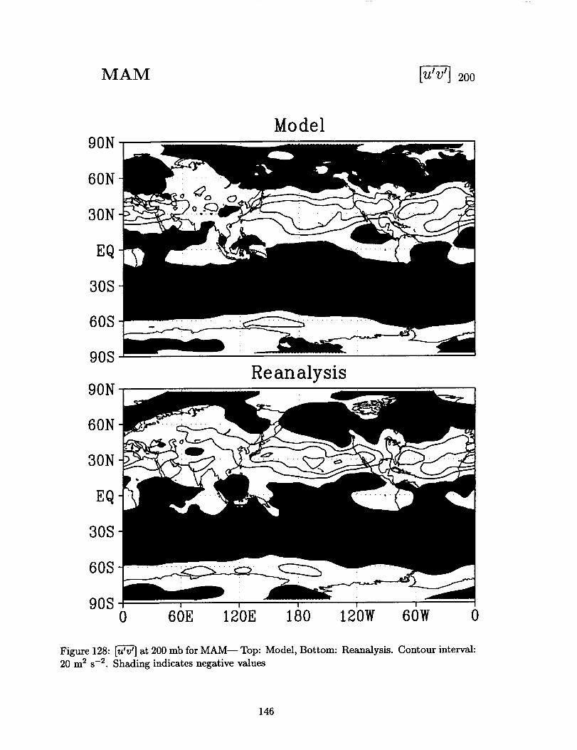
MAM [_ 200

90NModel

60N

30N

EQ

30S

60S

90S

90N

60N

30N

EQ

30S

60S

90S

Reanalysis

I I I I

0 60E 120E 180 120W 60W 0

Figure 128: [u_-rV-_at 200 mb for MAM-- Top: Model, Bottom: Reanalysis. Contour interval:

20 m 2 s -2. Shading indicates negative values

146

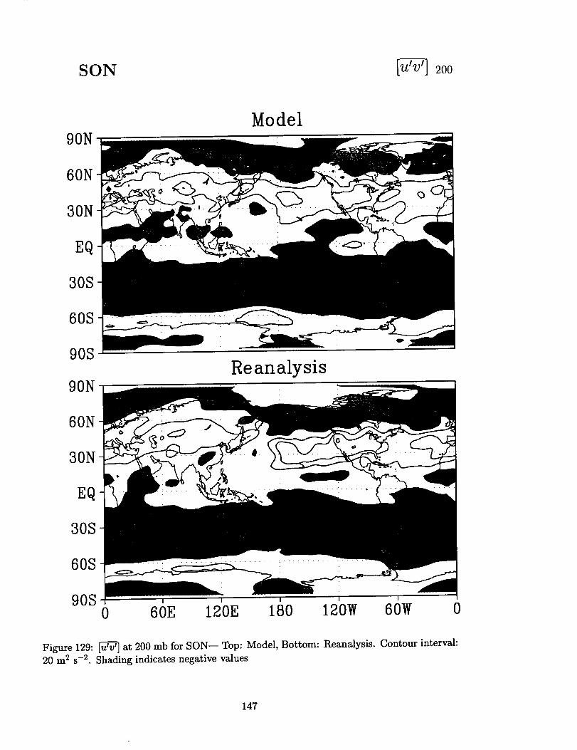
SON [_ 2oo

90N

60N

30N

EQ

30S

60S

90S

Model

90NReanalysis

60N

30N

EQ

30S

60S

90S , , , ' '0 60E 120E 180 120W 60W 0

Figure 129: [u--_Tv'] at 200 mb for SON-- Top: Model, Bottom: Reanalysis. Contour interval:

20 m 2 s -2. Shading indicates negative values

147

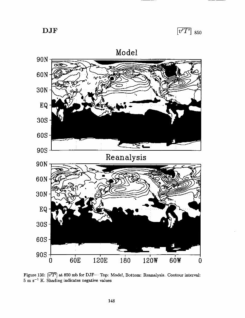
DJF _ 850

90NModel

60N

30N

EQ

30S

60S

90S

90NReanalysis

60N

30N

EQ

30S

60S

90S I I I I

0 60E 120E 180 120W 60W 0

Figure 130: [v'T _] at 850 mb for DJF-- Top: Model, Bottom: Reanalysis. Contour interval:

5 m s -1 K. Shading indicates negative values

148

JJA [_ 850

90NModel

60N

30N

EQ

30S

60S

90S

90N

60N

30N

EQ

30S

60S

90S

Reanalysis

| |

0 60E 120E 180 120W 60W 0

Figure 131: [v'T'] at 850 mb for JJA-- Top: Model, Bottom: Reanalysis. Contour interval:


149

MAM _-_ ss0

90N

Model

60N

30N

EQ

30S

60S

90S

90N

60N

30N

EQ

30S

60S

90S

Reanalysis

0 60E 120E 180 120W 60W 0

Figure 132: [v--_TT'] at 850 mb for MAM-- Top: Model, Bottom: Reanalysis. Contour

interval: 5 m s -1 K. Shading indicates negative values

150

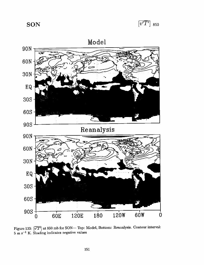
SON _ sso

90NModel

60N

30N

EQ

30S

60S

90S

90NReanalysis

I il lilli

60N

30N

EQ

30S

60S

90S I I I

0 60E 120E 180 120W 60W 0

Figure 133: [v-'rT_T_]at 850 mb for SON-- Top: Model, Bottom: Reanalysis. Contour interval:


151

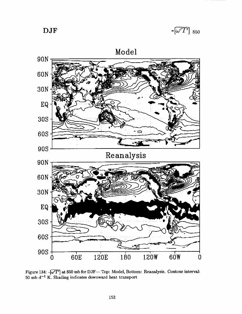
DJF -[J-_ sso

90NModel

60N

30N

EQ

30S

60S

90S

90N

60N

30N

EQ

30S

60S

90S

Reanalysis

!

0 60E 120E 180 120W 60W 0

Figure 134: -[w--}-_T'] at 850 mb for DJF-- Top: Model, Bottom: Reanalysis. Contour interval:

50 mb d -1 K. Shading indicates downward heat transport

152

JJA -[w-_ ss0

90NModel

60N

30N

E0

30S

60S

90S

90NReanalysis

60N

30N

EQ

30S

60S

90S0 60E 120E 180 120W 60W 0

Figure 135: -[w_T I] at 850 mb for JJA-- Top: Model, Bottom: Reanalysis. Contour interval:

50 mb d -1 K. Shading indicates downward heat transport

153

MAM -[_-_ 850

90NModel

60N

30N

EQ

30S

60S

90S

90N

60N

30N

EQ

30S

60S

90S I !

Reanalysis

0 60E 120E 180 120W 60W 0

Figure 136: -[w-'r_T_] at 850 mb for MAM-- Top: Model, Bottom: Reanalysis. Contour

interval: 50 mb d -1 K. Shading indicates downward heat transport

154

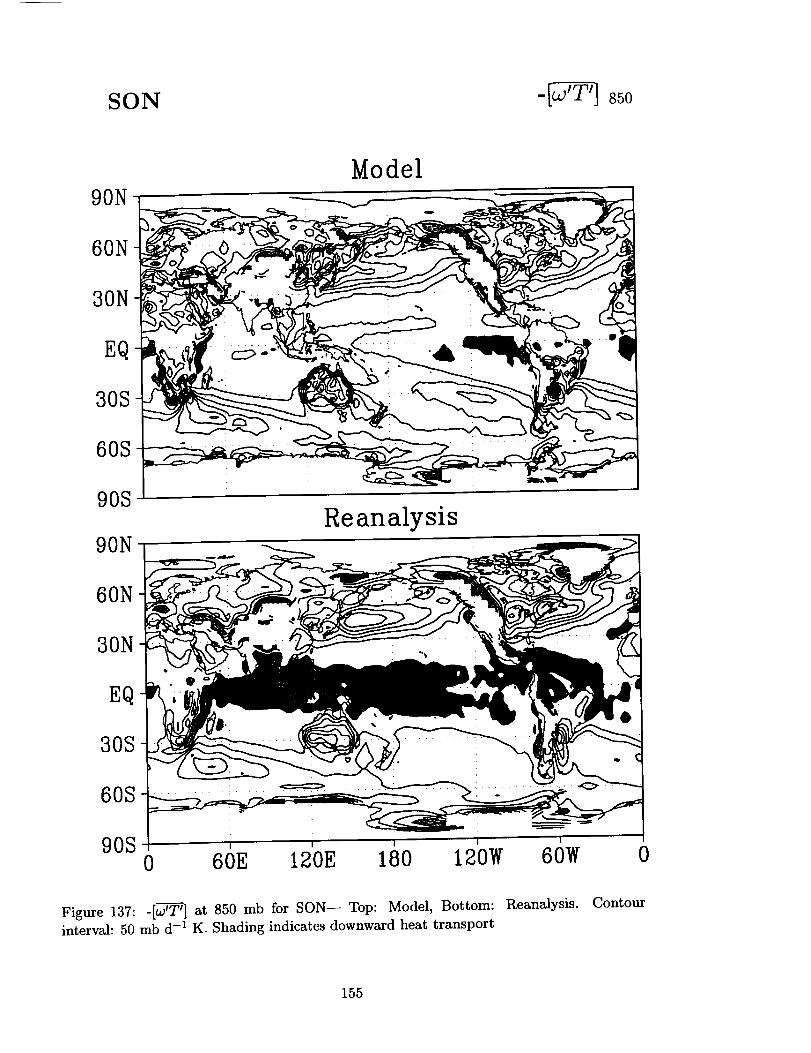
SON -[_ sso

90NModel

60N

30N

EQ

30S

60S

90S

Reanalysis90N

60N

30N

EQ

30S

60S

90S ! !

0 60E 120E 180 120W 60W 0

Figure 137: -[w-7_T'] at 850 mb for SON-- Top: Model, Bottom: Reanalysis. Contour

interval: 50 mb d -1 K. Shading indicates downward heat transport

155

DJF _q_ ss0

90NModel

60N

30N

nq

30S

60S

90S

90NReanalysis

60N

30N

EQ

30S

60S

90S0 60E 120E 180 120W 60W 0

Figure 138: [v-_ at 850 mb (ms -1 g kg -1) for DJF-- Top: Model, Bottom: Reanalysis.

Contour interval: 2 m s -1 g kg -1. Shading indicates negative values

156

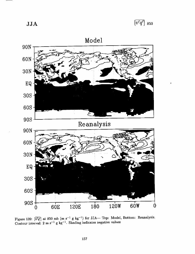
JJA _ 850

90N

60N

30N

EQ

30S

60S

90S

90N

Model

Reanalysis

60N

30N

EQ

30S

60S

90S I I

0 60E 120E 180 120W 60W 0

Figure 139: [v-_] at 850 mb (ms -1 g kg -1) for JJA-- Top: Model, Bottom: Reanalysis.

Contour interval: 2 m s-1 g kg -1. Shading indicates negative values

157

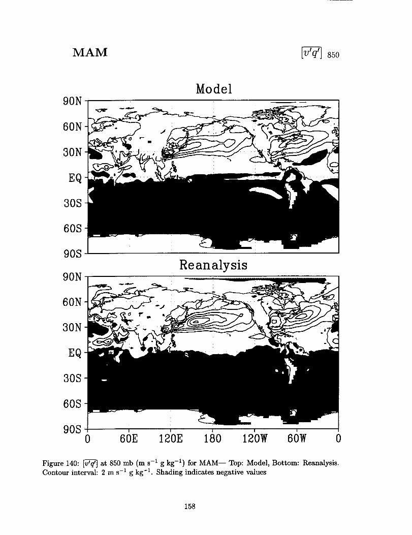
MAM _ 850

90NModel

60N

30N

EQ

30S

60S

90S

90NReanalysis

60N

30N

EQ

30S

60S

90S I I I

0 60E 120E 180 120W 60W 0

Figure 140: [v-_] at 850 mb (m s -1 g kg -1) for MAM-- Top: Model, Bottom: Reanalysis.


158

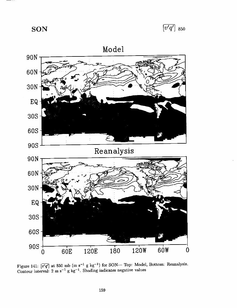
SON _ ss0

90NModel

60N

30N

EQ

30S

60S

90S

90NReanalysis

60N

30N

EQ

30S

60S

90S0 60E 120E 180 120W 60W 0

Figure 141: [v--_] at 850 mb (m S-1 g kg -1) for SON-- Top: Model, Bottom: Reanalysis.


159

160

GLOBAL MAPS OF PHYSICS DIAGNOSTICS


Precipitation

Total Precipitable Water

Outgoing Longwave Radiation

Longwave Cloud Radiative Forcing

Absorbed Solar Radiation

Solar Cloud Radiative Forcing

Net Radiation at the Top of the Atmosphere

Net Cloud Radiative Forcing

Zonal Surface Stress (_'x)

Meridional Surface Stress (Ty)

Curl of the Surface Wind Stress

Surface Sensible Heat Flux

Surface Latent Heat Flux

161

0e_

e_

e_

¢9

<

__JILl

o

_.JW

o

e-

tQ)

°_X

t--°_

I(13

°_X

00

©

_9

©

_9

I

_9

©

_9

d_Cq

_D

o

t_ •

_au

._ --_

162

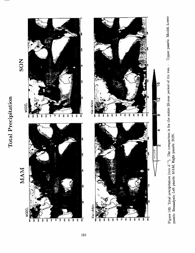
Z©

0o_ --.]

w

O

o_

o_

¢9

_._]W

O

C°_

I{D

°_X

©

o

L

_9

©

d_Cq

_9

_9

o

._

163

._1W

o

.__JW

0

o'1

_D

D

!

#

O 0

4_

O0

_9

O

o

¢D

a]

164

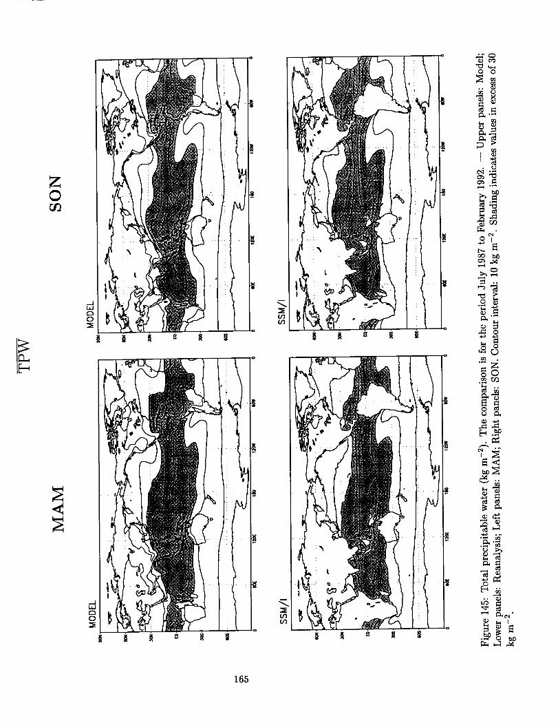
Z©

.--In,n

o

.--In,u

o"5

0 0

o?

_ o,

0 _

,_ o

0

0o

_._

_N

N

165

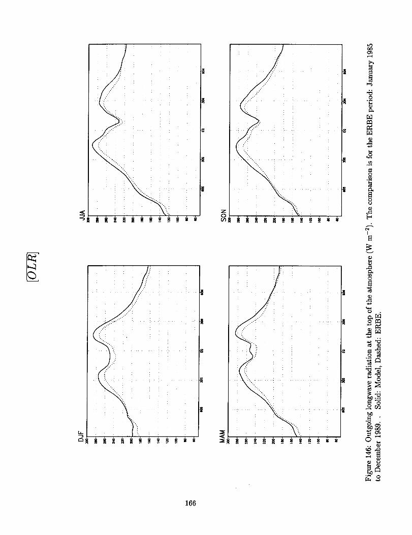
o

I-.4

o

o

I

t.4

o

t.*.4

o_

o

_D

°°

,3.)

O

166

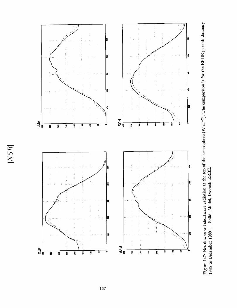
. ii

}

la.

.|

"I

/

. . .

"i

.£

¢)

o

8

I

_D

o

_D

o

<D

_o_Q

Z

O

_0oo°,'_

167

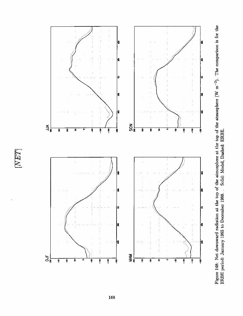
It-

§

izO

8

- 7 T

t-4

O

O

_D

I

_D

o

o

o

o

t*-4o

o

_D

0 o

o

168

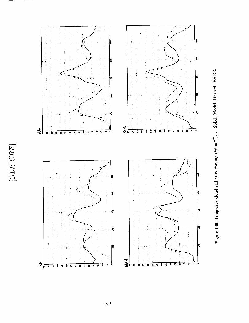
I

.-...-..a

: i i i

! ! i ! !

: !

o

or_

v

_0

@"d

o

169

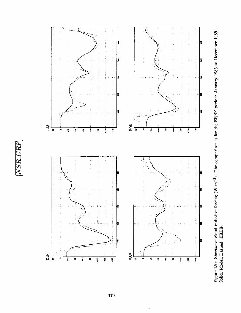
P--i

I

r_

,,<

.,. .....

i9..i .+o m, _p + +p s :_ ,

7 7 -

++,°++,++++_+,

°+++++++

t..*

o

OO

,--4

oo,..t

t.-*

o

o¢_

cq

I

.,.-t

o

u_

o

u'3 0

_D

• _ o_cn

170

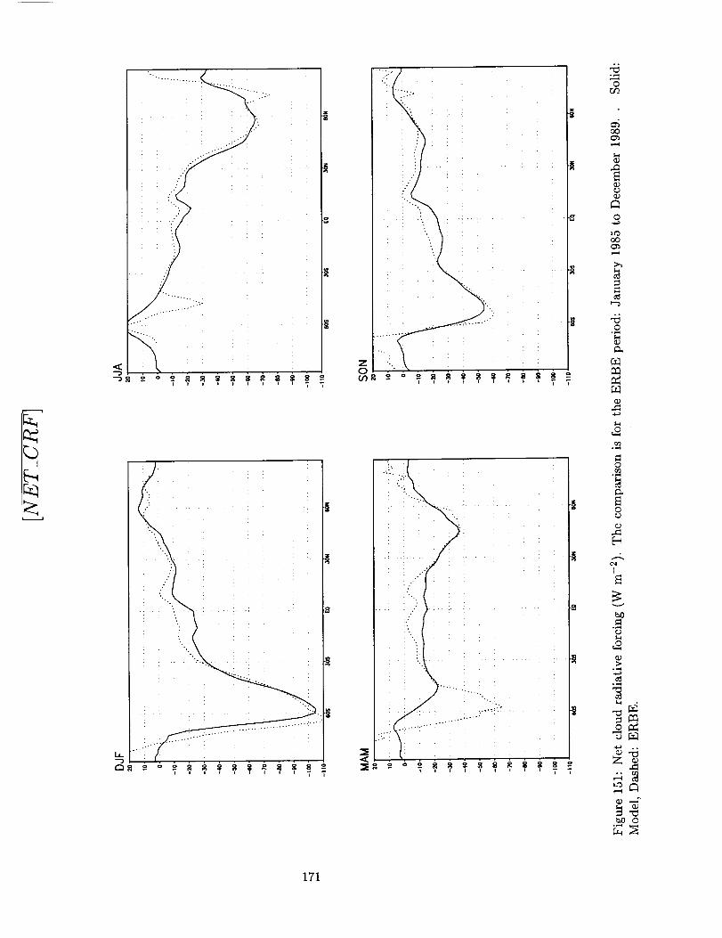
I

¢7

I I.- .-'"

la_

o

'o.

• ."_ i :.... i .......• i

". I . : : :

'_) ............. ,

or_

o

o

o

I

o_"d_

171

I

<

_Jw

0

__JW

0

wrnn_w

d

LFD

_XD

.o_Q

m

m<

s_

©

©

,--.i.° ,,_

172

]

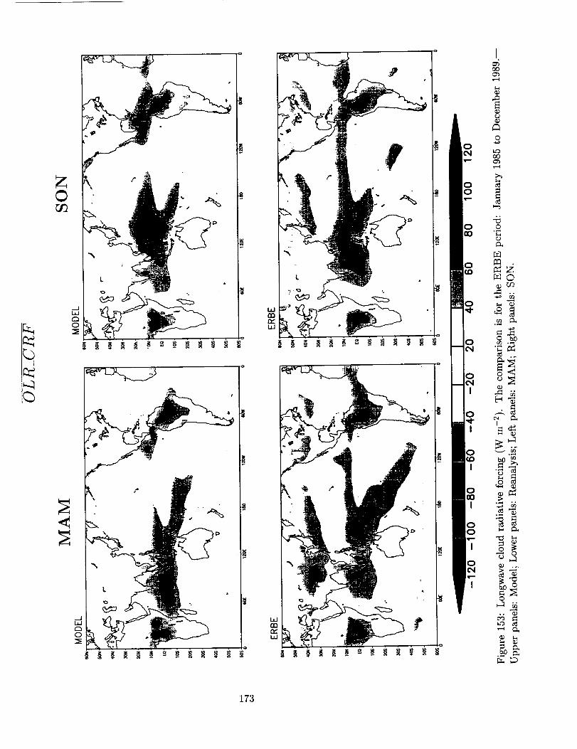
w

r_w

I

_J

©

xc_oo

_-_ °°

°_

I

o,-_

.,_

©

173

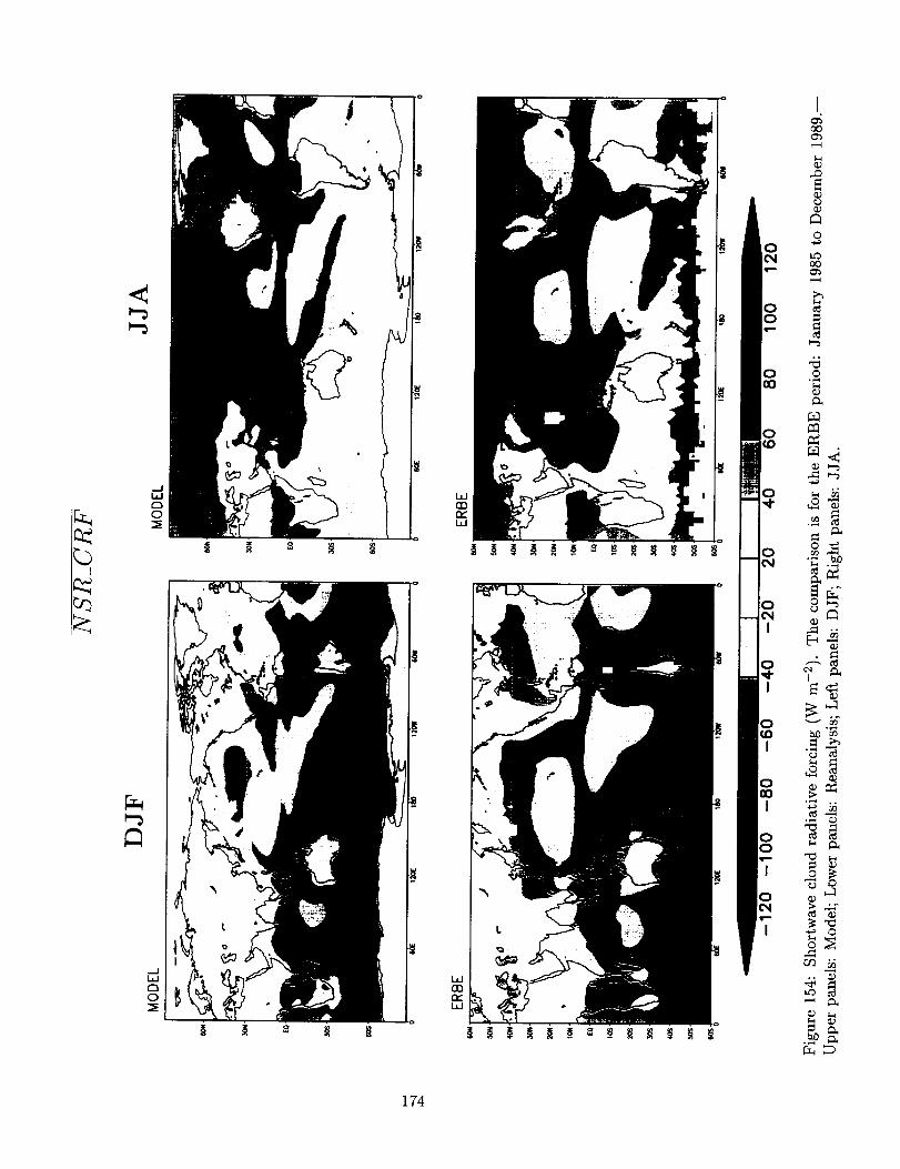
I

c_

<

LJ

o

o

Wrn

r_

w

r_w

I

_9,.Q

¢D

¢D

o

OO

cg

o

o _

• _

I

_'N

o_

-_ 0

174

I

Z©

._IW

o

.m

Wnnr_W

¥

W

nnr_L_

IoO

©

oO

.o

©

o

.m

175

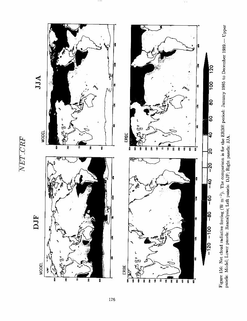
I

,¢

W

O

_..JWC_O

rn

f_W

L

m

f_w

¢D

]

_9

¢D

_9

©

O

¢D

c_

¢D

,._ o.

¢D

¢9 ¢6

¢D

°_

176

I

Z©

__JW

o

__JW

¢-_o-5

W

nnn_W

Wnnn_W

I

gI

I

I

©

.o

©

CD bO

o_

©

177

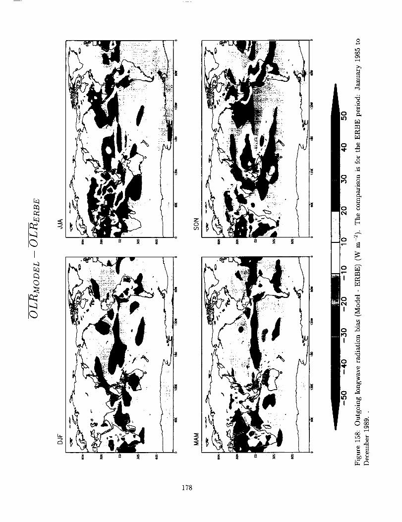
c_

I

C_

z0

178

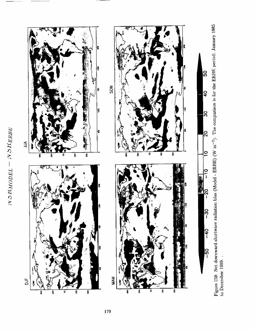
m:g

I

.<"0"0

.<

179

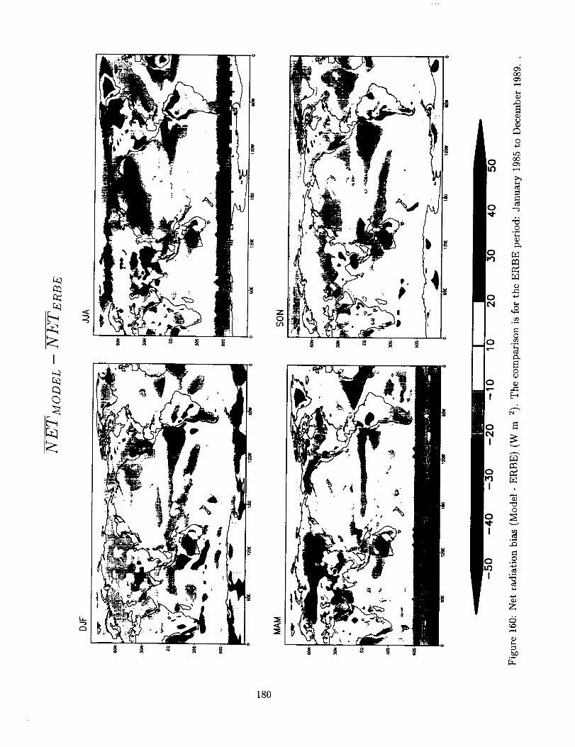
I

q)

n

i

180

This page left intentionally blank.

181

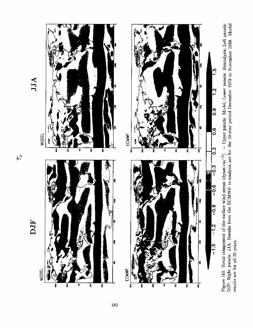
g_

._JW

0

_g

-..At.J

0

¢.2W

"5¢.2W

182

Z©

JWC_0

0

Id_

¢.}

¢.)W

183

<

-.Ji,it:30::E

d

II!

i,i

LIJ

t,I

:l

J4'

|

184

Z©

I,

(DW

¢.)W

185

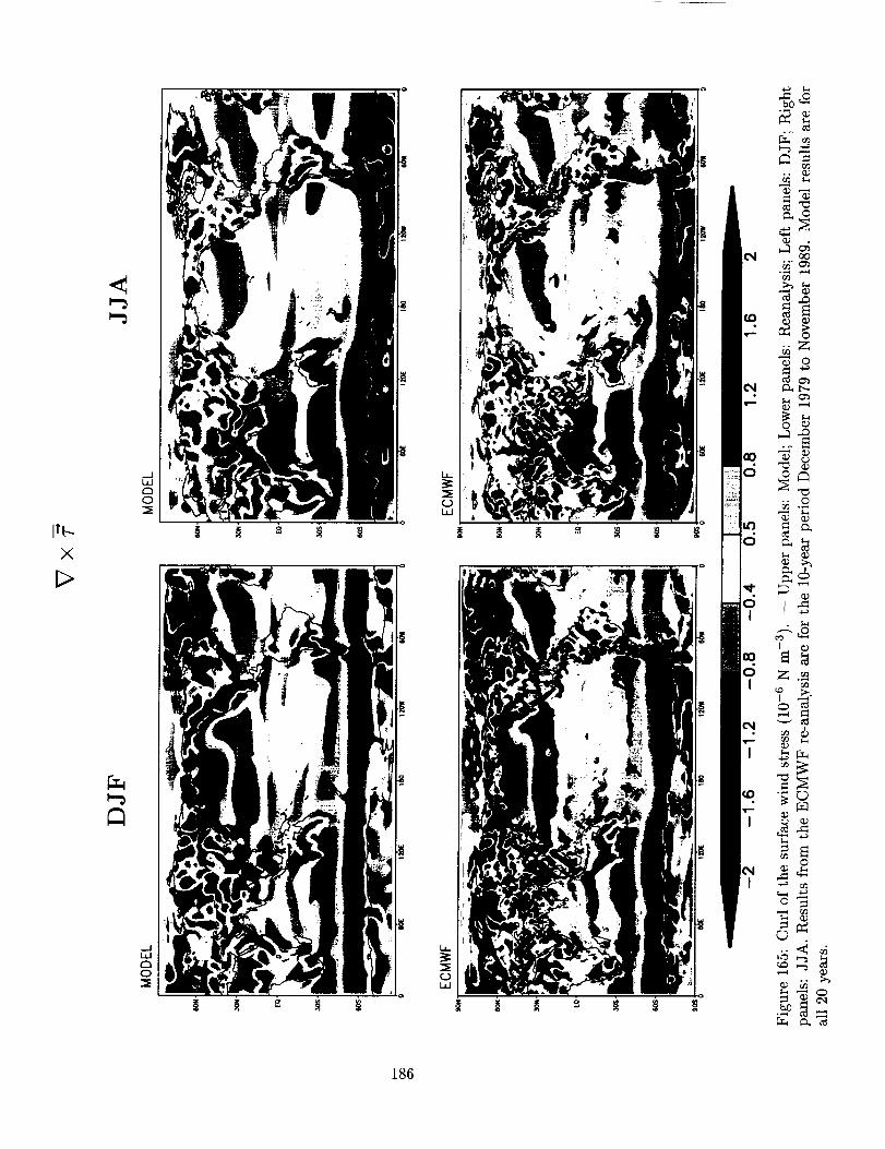
It_-

X

I>.

.<

i,itm0

._..IWC_0

I,

r,_)ILl

3:

_Z

186

<

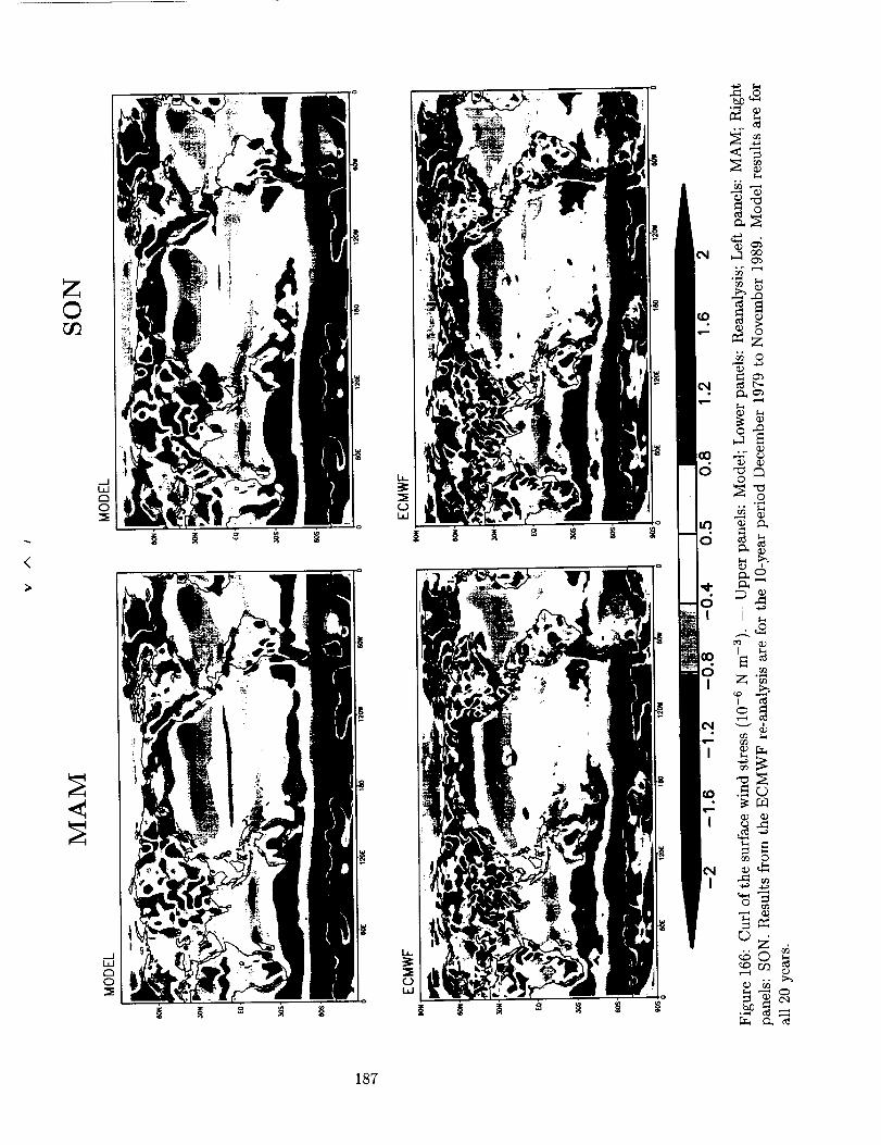
Z©

<

_Jt_

0

_JW

0

c.)

0W

187

<

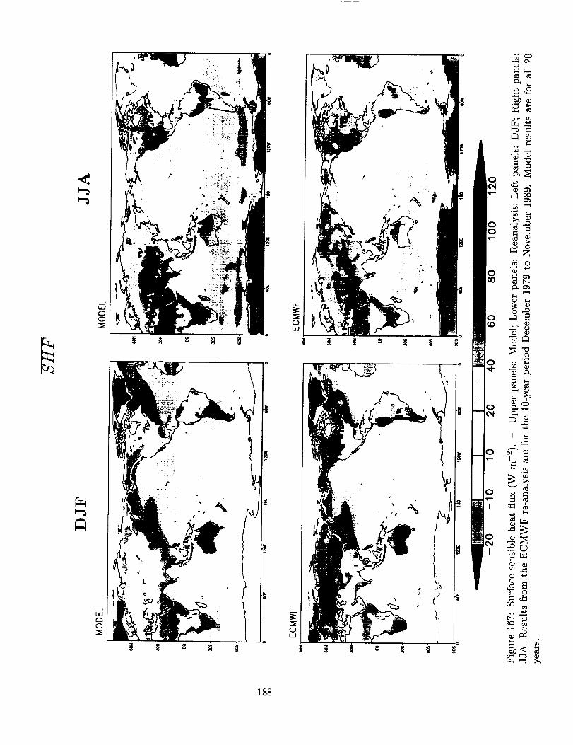
__IWa

0

W

0

I,

W

Ii,

W

0

©_z

o

,2..,_

©

"" _)

J_

r_

188

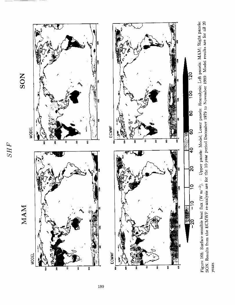
0r_

d

"5

.__lI,I

0

IJ_

(.3W

g

o

o

o

o

0

o

L)

r_

no

0

189

.¢

_...IW

O

%

t

.0 ¢_)

¢,q

o_

G

© ¢0

oo ,'_

o

n_¢5

¢q

o

°,.._

190

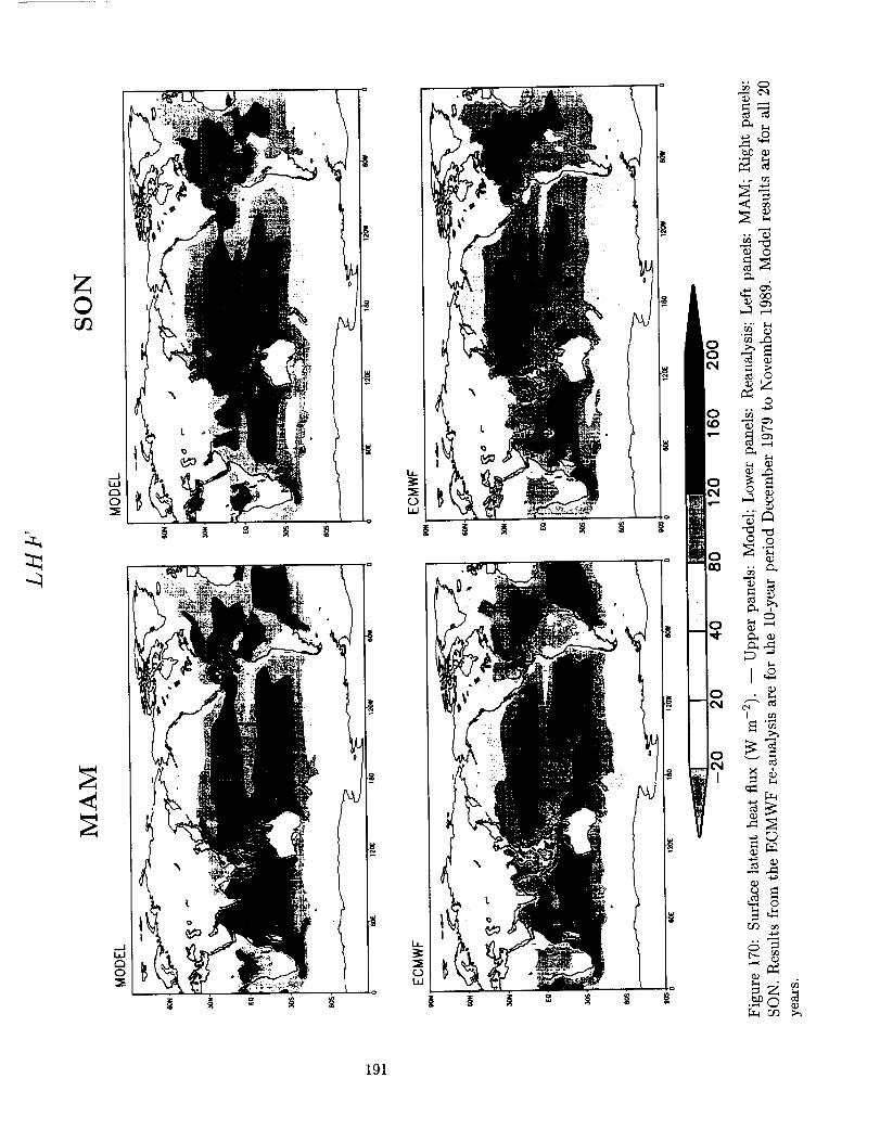
Z©

JW

0

/

P

tJ..I

191

192

Previous Volumes in This Series

Volume 1

September 1994

Volume 2

October 1994

Volume 3

December 1994

Volume 4

January 1995

Volume 5

April 1995

Volume 6

April 1995

Volume 7

September 1995

Volume 8

March 1996

Documentation of the Goddard Earth Observing System

(GEOS) general circulation model - Version 1

L.L. Takacs, A. Molod, and T. Wang

Direct solution of the implicit formulation of fourth order

horizontal diffusion for gridpoint models on the sphere

Y. Li, S. Moorthi, and J.R. Bates

An efficient thermal infrared radiation parameterization for

use in general circulation models

M.-D. Chou and M.J. Suarez

Documentation of the Goddard Earth Observing System

(GEOS) Data Assimilation System - Version 1

James Pfaendtner, Stephen Bloom, David Lamich,

Michael Seablom, Meta Sienkiewicz, James Stobie,and Arlindo da Silva

Documentation of the Aries-GEOS dynamical core: Version 2

Max J. Suarez and Lawrence L. Takacs

A Multiyear Assimilation with the GEOS-1 System:

Overview and Results

Siegfried Schubert, Chung-Kyu Park, Chung-Yu Wu,

Wayne Higgins, Yelena Kondratyeva, Andrea Molod,

Lawrence Takacs, Michael Seablom, and RichardRood

Proceedings of the Workshop on the GEOS-1 Five-YearAssimilation

Siegfried D. Schubert and Richard B. Rood

Documentation of the Tangent Linear Model and Its Adjointof the Adiabatic Version of the NASA GEOS-1 C-Grid GCM:

Version 5.2

Weiyu Yang and I. Michael Navon

193

Volume 9March 1996

Volume 10

April 1996

Volume 11

May 1997

Volume 12

August 1997

Volume 13

December 1997

Volume 14

August 1998

Volume 15

June 1999

Volume 16

November 1999

Energy and Water Balance Calculations in the Mosaic LSM

Randal D. Koster and Max J. Suarez

Dynamical Aspects of Climate Simulations Using the GEOSGeneral Circulation Model

Lawrence L. Takacs and Max J. Suarez

Documentation of the Tangent Linear and its Adjoint Modelsof the Relaxed Arakawa-Schubert Moisture Parameterization

Package of the NASA GEOS-1 GCM (Version 5.2)

Weiyu Yang I. Michael Navon, and Ricardo Todling

Comparison of Satellite Global Rainfall Algorithms

Alfred T.C. Chang and Long S. Chiu

Interannual Variability and Potential Predictability in Re-analysis Products

Wie Ming and Siegfried D. Schubert

A Comparison of GEOS Assimilated Data with FIFEObservations

Michael G. Bosilovich and Siegfried D. Schubert

A Solar Radiation Parameterization for Atmospheric Studies

Ming-Dah Chou and Max J. Suarez

Filtering Techniques on a Stretched Grid General CirculationModel

Lawrence Takacs, William Sawyer, Max J. Suarez,and Michael S. Fox-Rabinowitz

194

REPORT DOCUMENTATION PAGE J FormApprovedOMB No. 0704-0188

Public reporting burden for this collection of information is estimated to average I hour per response, including the time for reviewing instructions, searching existing data sources,gathering and maintaining the data needed, and completing end reviewing the collection of information, Send comments regarding this burden estimate or any other aspect of thiscollection of information, including suggestions for reducing this burden, to Washington Headquarters Services, Directorate for Information Operations end Reports, 1215 JeffersonDavis Highway, Suite 1204, Arlington, VA 22202-4302, and to the Office of Management and Budget, Paperwork Reduction Project (0704-0188), Washington, DC 20503,

I" AGENCYUSEONLY (LeBveblank) I2"REPORTDATEjuIy2000 T 3"REPORTTYPEANDDATESCOVEREDTechnicalMemorandum

4. TITLE AND SUBTITLE 5. FUNDING NUMBERSTechnical Report Series on Global Modeling and Data AssimilationVolume 17--Atlas of Seasonal Means Simulated by the NSIPP 1

---Atmospnenc GeM Code 970

6. AUTHOR(S) 971-622-24-47-26

Julio Bacmeister, Philip J. Pegion, Siegfried D. Schubert, and Max J. Suarez

7. PERFORMING ORGANIZATION NAME(S) AND ADDRESS (ES)

Oceans and Ice Branch

Goddard Space Flight Center

Greenbelt, Maryland 20771

9. SPONSORING / MONITORING AGENCY NAME(S) AND ADDRESS (ES)

National Aeronautics and Space Administration

Washington, DC 20546-0001

8. PEFORMING ORGANIZATIONREPORT NUMBER

2000-03740-0

10. SPONSORING I MONITORINGAGENCY REPORT NUMBER

TM-2000-104606, Vol. 17

11. SUPPLEMENTARYNOTES

J. Bacmeister: Universities Space Research Associates; P.J. Pegion: General Sciences Corporation, Laurel,

Maryland

12a. DISTRIBUTION I AVAILABILITY STATEMENT

Unclassified-Unlimited

Subject Category:46

Report available from the NASA Center for AeroSpace Information,

7121 Standard Drive, Hanover, MD 21076-1320. (301) 621-0390.

13. ABSTRACT (Maximum 200 words)

12b. DISTRIBUTION CODE

This atlas documents the climate characteristics of version 1 of the NASA Seasonal-to-lnterannual Prediction Project(NSIPP) Atmospheric General Circulation Model (AGCM). The AGCM includes an interactive land model (the Mosaicscheme), and is part of the NSIPP coupled atmosphere-land-ocean model. The results presented here are based on a20-year (December 1979-November 1999) "AMIP-style" integration of the AGCM in which the monthly-mean sea-surfacetemperature and sea ice are specified from observations. The climate characteristics of the AGCM are compared with theNational Centers for Environmental Prediction (NCEP) and the European Center for Medium-Range Weather Forecasting(ECMWF) reanalyses. Other verification data include Special Sensor Microwave/lmager (SSM/I) total precipitable water,the Xie-Arkin estimates of precipitation, and Earth Radiation Budget Experiment (ERBE) measurements of short and longwave radiation. The atlas is organized by season. The basic quantities include seasonal mean global maps and zonal andvertical averages of circulation, variance/covariance statistics, and selected physics quantities.

14. SUBJECT TERMSNumerical Methods, Atmospheric Models, Regional Models, Climate ModelsAtmospheric General Circulation

17. SECURITY CLASSIFICATIONOF REPORT

Unclassified

NSN 7540-01-280-5500

18. SECURITY CLASSIFICATIONOF THIS PAGE

Unclassified

19. SECURITY CLASSIRCATIONOF ABSTRACT

Unclassified

15. NUMBER OF PAGES192

16. PRICE CODE

20. LIMITATION OF ABSTRACT

UL

Standard Form 298 (Rev. 2-89)

Documents

Technical Report Series on Global Modeling and Data ... · PDF fileNASA/TM-2000-104606, Vol. 17 Technical Report Series on Global Modeling and Data Assimilation Max J. Suarez, Editor