Technical Report CSTN-101

Visualising Volumetric Fourier Transforms of Asymmetric 3DGrowth Models

Ken A. Hawick, Arno Leist and Daniel P. PlayneComputer Science, Institute for Information and Mathematical Sciences,

Massey University, North Shore 102-904, Auckland, New ZealandEmail: k.a.hawick, a.leist, d.p.playne @massey.ac.nz

Tel: +64 9 414 0800 Fax: +64 9 441 8181

September 2011

ABSTRACT

Volumetric visualisation of Fourier spectral data is apowerful but computationally intensive tool for under-standing growth models. Visualising frequency-domainspectral representations of simulation model variablesthat are normally defined on a spatial mesh can be a use-ful aid to understanding time evolutionary behaviour.While it is common to study the symmetric or spheri-cally averaged FFT of models, we consider renderingthe full 3D FFT representations in interactive time. Weuse volume rendering methods to study the FFT andalso consider asymmetric model cases where sphericalaveraging would be misleading. We discuss visualisa-tion of Fourier-transformed data fields and some tech-niques for analysing and interpreting them. We presentsome application examples and implementations of ren-dering iso surfaces in the spectral scattering represen-tation of of the normal and small-world rewired Isingmodel using Graphical Processing Units(GPUs) that al-low both simulation and rendering to be achieved in in-teractive time.

KEY WORDS3D Fast Fourier Transforms; spectral model representa-tion; GPU computing; volumetric visualisation.

1 Introduction

A commonly recurring problem in scientific visualisa-tion is to “see inside” a block of three dimensional datathat is associated with a simulation model. Many phys-ical and engineering models in materials science, fluiddynamics, chemical engineering and other application

areas including medical reconstruction [1] fit this prob-lem pattern.

Volume rendering [2–4] is a relatively long standingproblem in computer graphics [5] with a number ofapproaches for “seeing into volumes” [6] and for pro-viding visual cues into volumes [7] having been ex-plored. Approaches vary from identifying the surfacespresent [8] in the interior of a data volume [9] and eithercolouring them or texturing [10] them accordingly.

It is often hugely useful to a scientific modeller to beable to visualise an interactively running model and ex-periment with different parameter combinations prior tocommitting computational resources to detailed statisti-cal investigations. The visualisation often leads to someinsight into a particular phenomena that bears close nu-merical study or might lead to a hypothesis or expla-nation as to a numerical observation such as a phasetransition or other critical phenomena. Some data mod-els require visualisation of complex data fields that mayhave vector elements [11] or complex numbers [12].We focus solely on scalar voxel element data and in thecase of the complex numbers that arise from FFT datawe visualise as separate real or imaginary parts, or moreusefully as the normalised amplitudes.

In recent times the notion of computational-steering[13] has been identified as attractive to users, as has thepotential use of remote visualisation [14] to link fastgraphics processing devices to high-performance com-pute systems to enable interactive real time simulationof large scale model systems with associated real timevolume rendering [15] or visualisation [16]. To thisend data-parallel computing systems such as the MAS-PAR [17] and other specialist hardware [18] were onceemployed.

1

An obvious continued goal is to incorporate on-demandhigh-performance simulation into fully interactive vir-tual reality systems [19]. While this goal is still someeconomic way away for desktop users, modern GPUsdo offer some startling performance potential for bothcomputation [20–22] and volume visualisation [23] forinteractive simulations in computational science.

In this paper we consider some of the recent high-performance hardware capabilities of GPUs and justas importantly recent software developments that haveled to programming languages for accelerator deviceslike NVIDIA’s Compute Unified Device Architecture(CUDA) [24]. GPUs can help accelerate the numericalsimulation as well accelerate the rendering performanceof the graphical system. Together, these two capabili-ties allow exploration of model systems that are largeenough and yet can be simulated fast enough in interac-tive time, to spot new and interesting phenomena.

The application example we visualise in this paper isthe well known Ising model of a computational mag-net [25]. This model has been very well-studied numer-ically in two and three dimensions and also graphicallyin two dimensions. We harness the power of GPUs toshow how both the computations and the graphical ren-dering can be accelerated sufficiently so that a systemof sizes up to around 2563 individual spin cells can besimulated interactively. We add small-world link re-wirings to the model to experiment with visualisationof asymmetric model systems in the spectral represen-tation.

Our article is structured as follows: In Section 2 we dis-cuss the meaning and interpretation of a discrete Fouriertransform of a model such as the Ising system. We de-scribe how the Fourier field in 3D can be visualised andappropriately rendered in Section 3. We give a briefsummary of pertinent aspects of the GPU that enableinteractive time computation of FFTs and visualisationin Section 4. We present a set of rendered screen-dumpsand spherical averaged data plots in Section 5 to showhow the rendering exposes the asymmetry from modelperturbations such a s small-world shortcut re-wirings.We offer some discussion of the results in Section 6 andconcluding remarks and areas for further developmentof these techniques in Section 7.

2 Fourier Spectral Fields

Direct visualisation of field data can often be aug-mented by examination of the Fourier transformed field.A number of particle scattering techniques involvingelectrons or neutrons are commonly used in materialsscience experimentation. These techniques yield a scat-

tering pattern that is mathematically equivalent to theFourier transform of the atomic pattern of the sample.A similar “numerical scattering” approach can be em-ployed [26,27] to represent the bulk properties of a sim-ulated model. The scattering pattern formed by collect-ing the scattered particles in suitable detectors can givequantitative indications of the size and sometimes shapeof spatial fluctuations and structures that are forming inthe material. In the numerical simulation, a computa-tion of the scattering pattern is possible and this canreveal properties of the simulated data field that wouldotherwise be hard to extract and observe. We give abrief derivation of the scattering formula.

A neutron scattering experiment conducted on a samplewith volume V with scattering angle Ω and scatteringcross-section (probability) of σ is given by:

dσ

dΩ≈ (ρp − ρm)

2 1

V

∣∣∣∣∫V

eiQ.rdr

∣∣∣∣2 (1)

The term (ρp − ρm)2 is the difference between the den-

sities of the phase of interest and the background den-sity and is known as the small angle scattering contrast,denoted as 4ρ2. A large value of 4ρ2 gives higherrelative scattering intensity from the precipitate phase.Equation 1 can then be rewritten as:

dσ

dΩ≈ (ρp − ρm)

2 1

VS(Q) (2)

which defines the structure function as:

S(Q) =

∣∣∣∣∫V

eiQ.rdr

∣∣∣∣2 (3)

which is strictly a dimensionless quantity.

In material science it would be usual to factor out var-ious bulk constants and volume factors to separate thescattering intensity I from the the structure function.For the purposes of this paper, we can treat the S(Q)as the same as the scattering intensity and which cor-responds to the Fourier transform of the “contrast” orthe physical configuration in the model system. Wecan take the contrast as simply the value of the field.So S(Q) or I(qx, qy) can be computed by a two-dimensional Fast Fourier Transform (FFT) of the simu-lated model data field u.

The Fourier transform of wholly real data such as forthe scalar field of the Cahn Hilliard system on a sym-metric geometry is also symmetric and it is commonto spatially shift it to show the centred scattering pat-tern. We can visualise a movie time sequence of FFTdata in much the same way as we visualise the directmodel field. In the case of a symmetric scattering pat-tern, no one dimension is dominant and it is also pos-sible to make a spherical average (or circular average

2

in 2 dimensions). Various properties such as the char-acteristic length scale and effective dimensions of theinternal model structures can be obtained from an anal-ysis of the position of peaks and the fitted power-lawsof these averaged scattering curves [28, 29].

The new contribution we explore in this present pa-per however involves treating the full three dimen-sional scattering pattern as a data set we can colour,fly through and visualise looking for features and iso-surfaces.

The multi-dimensional discrete Fourier TransformH isdefined: where the l’th dimension is subdivided into Nldiscrete values and nl and kl range from 0...Nl − 1.

For our purposes in this present paper we use three di-mensional transforms and N1 = N2 = N3 = 2p sothat the standard fast Fourier Transform library routinesfor CPU and GPU work straightforwardly without theneed for explicit data padding. In effect we are trans-forming a complex function h defined on a 3D mesh inphysical space and transforming it to its correspondingcomplex function H defined on a mesh in spatial fre-quency space. Spatial “frequencies” are usually knownas wave-numbers, and we defineQ = 2π/λ for a wave-length λ.

The spatial model we are focusing on in this paper is theIsing model of spins that are located on a spatial grid.In taking the FFT of the Ising spins we are effectivelycomputing a scattering pattern from the spatial arrange-ment of spins. This is analogous to measuring the actualneutron scattering from a single perfect magnetic crys-tal. Due to the symmetry properties of FFTs, the trans-form of a wholly real function has some twofold redun-dancy in the transform. Phase information is introduced– the transform consists of complex numbers with botha real and an imaginary part, but the transformed val-ues are mirror imaged in each dimension. Large lengthscale features in the original spatial data correspond toshort spatial frequencies in the transformed data.

In a growth model system such as the Ising model, aquench experiment starts off with a noisy system withnoise on all length scales. As the system is quenched,small domains form rapidly - corresponding to longspatial frequencies. As the system anneals and thesesmall domains grow, these long wavelengths corre-spondingly shorten. The scattering probability (distri-bution) of wave-numbers will typically start out flat,then develop a peak corresponding to the reciprocal ofthe most commonly occurring length scale in the ma-terial. The location of the peak typically decreases inwavenumber as the time annealing growth process con-tinues.

It is difficult to track a three-dimensional system visu-

ally and reliance in normally placed on the size char-acterisation of the separating phases by spherically av-eraged Fourier transforms (or circular averages on 2Dscattering patterns). The peaks vary considerably inmagnitude, but the peak positions can be well deter-mined, and mapped to characteristic domain sizes.

This much is known from standard small angle scatter-ing experiments on real materials. In this present paperhowever we are able to examine the full 3D transform asit changes in time and furthermore to examine asymme-tries that correspond to asymmetric growth phenomena.

The Ising model is a discrete spin model that exhibitsinteresting phase transitional properties. We have ex-perimented with a number of visualisation techniquesfor the 3D Ising system including cut away sections[30]. Spectral methods can also be applied to the Isingsystem and a particularly interesting area of study isthe effect of long range small-world re-wirings to theregular nearest neighbour lattice [31]. The unaveragedFourier Transform of the Ising system yields an effec-tive scattering pattern which in turn reveals the lengthscales present in the Ising system. This is especiallyuseful because these scattering patterns can be addedtogether to get a meaningful average, which is not pos-sible in the spatial domain.

The Ising model gives rise to a bit field s(x, y, z) whichwe transform to obtain the spatial structure functionS(qx, qy, qz), where we follow the literature conven-tion and use Q = (qx, qy, qz) for the wavenumber.These are the spatial analogies of the h(t) and H(f)functions described above in equation 4 in more con-ventional time-frequency notation. We are interested inthe location of features in wavenumber space and thesewill suggest (reciprocal) length scales that are pertinentto the spatial structure and growth going on inside theIsing bit field.

The transform we obtain in 3D is a set of complex num-bers, but it is useful to interpret them as scattering inten-sities so we take the norm of each cell thus combiningits real and imaginary parts and losing the phase. Whenaveraging over many independent simulation runs wecan directly average intensities with the interpretationof enhancing the scattering beam signal strength. Wethus have a 3D field of (real) scalar intensity numbersto visualise.

3 Visualisation Methods

When visualising a three-dimensional FFT, the usualchallenges of visualising a three-dimensional field areencountered. FFT transforms of a single system have

3

H(n1, n2, ..., nl) =

Nl−1∑kl=0

· · ·N2−1∑k2=0

N1−1∑k1=0

e2πiklnl/Nl · · · e2πik2n2/N2e2πik1n1/N1h(k1, k2, ..., kl) (4)

both a real and imaginary part which can further com-plicate the visualisation. Features and structure inFourier space data reflect characteristics of the real-space field. We visualise the magnitudes of the complexFourier values averaged over many simulations, the av-erages produce Fourier data representative of the entiremodel rather than one individual system. Visualisingthese averaged magnitudes rather than a single FFT re-duces the data to be visualised from a complex field toa scalar field.

A number of different methods are available for visu-alising a scalar field such as this. The visualisationmethod selected for analysing these FFTs is construct-ing and rendering iso-surfaces. Various ISO values canbe used to construct different iso-surfaces within theFFTs. Cycling through these different iso-surfaces canreveal the internal features and structure of the FFTs.

We use the marching cubes algorithm [32] to constructa polygon representation of the iso-surfaces. This al-gorithm generates a polygon surface representing theiso-surface in the FFT and has been implemented onthe GPU using CUDA. The GPU implementation canaccelerate the processing speed and also avoid unneces-sary data transfer between the GPU and the host CPU.

Once the surfaces have been created, they can be ren-dered using either a flat or smooth shading model.Smooth shaded polygon surfaces will appear more likethe smooth iso-surfaces they approximate. However,as with any visualisation, care should be taken thatthis graphics interpolation does not introduce any incor-rect information into the rendered image. Algorithm 1shows the two methods of calculating the normals. Theflat shading implementation computes a single normalfor each face while smooth shading computes a normalfor each vertex. The renderings in Figure 1 and Figure 2both use the flat shading model.

4 Graphical Processing Units &CUDA

Data parallel and array processing computer systemsare typically well suited to the highly regular computa-tional structure of Fast Fourier Transforms and volumerendering. Systems such as the DAP [33,34], MASPAR[35, 36] and Connection Machine [37] all had highlyoptimised FFT library routines in the 1980s and early

Algorithm 1 Calculating normals for smooth shadingof an iso-surface produced by the Marching Cubes al-gorithm. Note that × denotes the cross product opera-tion.

declare vertexes[], faces[], normals[]vertexes ← iso-surface vertexes from marchingcubesfaces← iso-surface faces from marching cubes//Flat Shadingfor all f in faces do

declare d0, d1, nd0← vertexes[f.i1]− vertexes[f.i0]d1← vertexes[f.i2]− vertexes[f.i0]n = d0× d1normals[f ]← n

end for//Smooth Shadingfor all f in faces do

declare d0, d1, nd0← vertexes[f.i1]− vertexes[f.i0]d1← vertexes[f.i2]− vertexes[f.i0]n = d0× d1normals[f.i0]← normals[f.i0] + nnormals[f.i1]← normals[f.i1] + nnormals[f.i2]← normals[f.i2] + n

end for

1990s. This capability is now available for highly data-parallel processing accelerators in the form of Graphi-cal Processing Units (GPUs) [38].

To keep up with the demands of the 3D games and ren-dering industries, Graphical Processing Units (GPUs)have been designed for very high compute through-put using increasingly parallel processing architectures.A current generation NVIDIA GPU (GTX-580), con-tains up to 16 streaming multiprocessors (SMs), eachof which contains 32 scalar processors (SPs), and canhandle millions of threads that are managed and sched-uled by the GPU hardware.

Threads are grouped into thread blocks of up to 1024threads (512 for older devices), which are then executedon the SMs. A thread block is further sub-divided intoblocks of 32 continuous threads called warps. At ev-ery instruction issue time, a warp scheduler issues aninstruction to a warp that is ready to execute. All thethreads in the warp either execute this instruction or areindividually disabled if they diverge at a data-dependentconditional branch. Full efficiency is thus only achievedwhen all 32 threads agree on the execution path. This is

4

a common challenge when developing on data-parallelarchitectures.

CUDA devices have a large global memory, a numberof fast on-chip memory areas including texture cache,constant memory cache and shared memory, as well asa set of 32-bit registers for each SM. The latest gen-eration of NVIDIA devices provides an additional L2cache, which is shared among all multiprocessors, aswell as an L1 cache that takes up part of the sharedmemory on each individual SM. The L1 and L2 cachesare used to cache global memory accesses and tem-porary register spills. Global memory is by far theslowest memory on the device and the fast on-chipcaches should be utilised where possible to improveperformance. Global memory bandwidth can be sig-nificantly improved when the threads of a (half-)warpaccess memory addresses within the same segment ofglobal memory (various restrictions apply depending onthe compute architecture of the device).

We use CUDA to harness this massively parallel com-pute power provided by todays commodity GPUs tooffload the main workload of our simulations to thegraphics device. This allows us to simulate much largersystems than otherwise feasible. Although we haveused CUDA and GPUs to do the simulation calculationsthemselves [39], we focus in this present paper on thevolume and FFT processing.

To perform the spectral analysis described in this paper,we utilise NVIDIA’s CUDA Fast Fourier Transform(CUFFT) library to compute the Fourier Transform inparallel on the GPU. This solution is particularly ap-pealing because the input data to the FFT, generated bythe simulation, already resides in graphics memory andthus does not need to be copied between the host andthe graphics card. CUDA can be used to perform all theprocessing required to compute the FFT for the currentsystem state (e.g. the spins of the Ising model) in paral-lel: (1) convert the input data structure into the formatrequired by the CUFFT library; (2) compute the FourierTransform; (3) compute the magnitudes and shift thedata to center it.

5 3D FFT Results

We present some illustrative screen-dumps of the 3DFFTs of various 3D Ising model configurations.

Figure 3 illustrates how the spherical mean of the 3DIsing model’s Fast Fourier Transform (FFT) changeswith the number of Metropolis update steps performed.The figure also shows the effects of introducing small-word re-wirings, which change the distances between

individual cells in the model. The increasing domi-nance of the lower frequency components in the regularlattice Ising system as the simulation progresses rep-resents the growth of tightly packed clusters with likespins.

The introduction of small-world rewired long distancelinks in the x-dimension speeds up the formation ofclusters, but it also increases the variance in the mag-nitude of the frequency components.

When edges are only rewired in the x-dimension, thenthis means that the y- and z-coordinates of the currentneighbour are “frozen” and only the x-value is ran-domly modified. The total number of rewired edgesthus remains the same—on average—for a given re-wiring probability P , no matter if the selection of newneighbours is restricted to certain dimensions or not.The hyper-surfaces for Ising systems rewired only inthe x-dimension are given in Figure 2.

The shape of the hyper-surfaces for the irregular sys-tem configuration easily explains the large error in themeasurements of the spherical mean. Limiting the re-wiring to the x-dimension reduces the distance betweencells in this dimension only, which produces a disk-likeshape (the center value is the constant of the FFT andhas been set to 0 as it is of no interest to us) for largeISO values, and a growing hole in the middle of thedisk for even larger ISO values. The explanation forthe disk-like shape is that the magnitude increases lesssteeply for the lower frequencies in the x-dimension asit does in the other dimensions. The hole increases insize when the magnitude in the y- and z-dimensions islarger than at any frequency in the x-dimension.

6 Discussion

The tightly packed clusters, or lumps of like spins, de-tected by the FFT are similar to what we would perceiveas a cluster when looking at a graphical representationof the system. However, Figure 4 shows that the actualsize distribution of the connected components looksquite different. After only one simulation step, whenthe system is still mostly random, almost all the cells arepart of one of the two major clusters, one for “up” spinsand the other for “down” spins. This is because with 6edges connecting every cell to its neighbours (exactlyfor P = 0.0 and on average for P > 0.0), it is possibleto reach almost all other cells with the same spin valuefrom any given source cell. The spectral analysis doesnot know about these connections and only looks at thespatial distribution of spin values.

When the temperature T is lower or near the critical

5

Figure 1: 3D FFT of the Ising model with a regular lattice after 256 simulation steps. T = 4.5115, ISO values (topleft to bottom right) are 0.02, 0.03, 0.04, 0.10, 0.70, 0.90.

Figure 2: 3D FFT of the Ising model with re-wiring only in the x-dimension after 256 simulation steps. P = 0.01,T = 4.55, ISO values (top left to bottom right) are 0.03, 0.06, 0.08, 0.11, 0.70, 0.90.

6

Figure 3: The spherical mean of the 3D FFT computed after 1, 2, 4, . . . , 1024 simulation steps of the Ising modelusing the Metropolis update algorithm. The system size N = 1283. The plot on the left shows the results for theregular cubic lattice Ising model with temperature Tc ≈ T = 4.5115. The plot on the right illustrates rewired irregularlattice Ising models with re-wiring probability P = 10−2 and Tc ≈ T = 4.55, where the arcs were randomly rewiredonly in the x-dimension. Each data point represents the mean value of 1000 simulation runs. The error bars illustratethe standard deviations. The error has been rescaled by a factor of 0.1 for frequency f = 20 for the plot on the right.

temperature Tc, then the system becomes less and lessrandom the more update steps are performed. Lumps oflike spins form and grow in size, which shows up withan increase in magnitude for the lower frequencies inthe FFT results. The distributions for the size of con-nected clusters, on the other hand, broaden around themedian of the system size until they eventually becomebimodal, with distinct peaks for the “up” and “down”spin clusters. The bimodal behaviour suggests that thechosen temperatures are lower than the respective crit-ical temperatures. If the temperatures are slightly in-creased to T = 4.52 for the regular lattice system or toT = 4.6 for the rewired system with P = 10−2, whichare above the respective critical temperatures, then thecluster size distributions retain a single peak in the equi-librated system.

The much quicker broadening of the cluster size distri-butions for P = 10−2 as compared to P = 0.0 sup-ports the intuitive assumption that the rewired connec-tions facilitate domain growth. While the shape of theregular lattice distribution still changes between steps1024 and 4096, no significant changes can be observedafter 1024 simulation steps for the rewired system. TheFFT results may appear to contradict this conclusion,as the low frequencies are less dominant in the rewiredsystem than in the regular lattice system. However, itneeds to be considered that a large cluster in the rewiredsystem is likely to consist of two or more spatially sep-arated smaller clusters that are only weakly connectedby a few long distance links, which is not picked up by

the spectral analysis.

Another interesting effect clearly visible in the resultsfor the rewired system is that after the distributions ini-tially become more and more front-heavy, this effectreverses after about 64 simulation steps and the distri-butions become flatter again. This is likely to be due toindividual clusters beginning to join together to largerclusters of different shapes, which changes the scatter-ing patterns produced by the FFT.

7 Conclusion

We have shown how 3D FFTs can be computed in in-teractive time and used to visualise structural propertiesof complex 3D data models such as the Ising model.We have also explored the asymmetries that occur whensmall-world re-wirings are inserted into the Ising modelsimulation model – in a single spatial direction. Theasymmetric structure and growth properties are clearlyvisible in the 3D FFT volumetric visualisation whereasthey are too subtle to see in the original real-space vol-umetric rendering.

This volumetric visualisation has traditionally been toocomputationally expensive to carry our interactively. Inpractice it ha s been of comparable or greater compu-tational cost than the simulation itself and so has beena neglected technique. Using GPUs and data parallelprocessing techniques, we have found hat it is viable in-

7

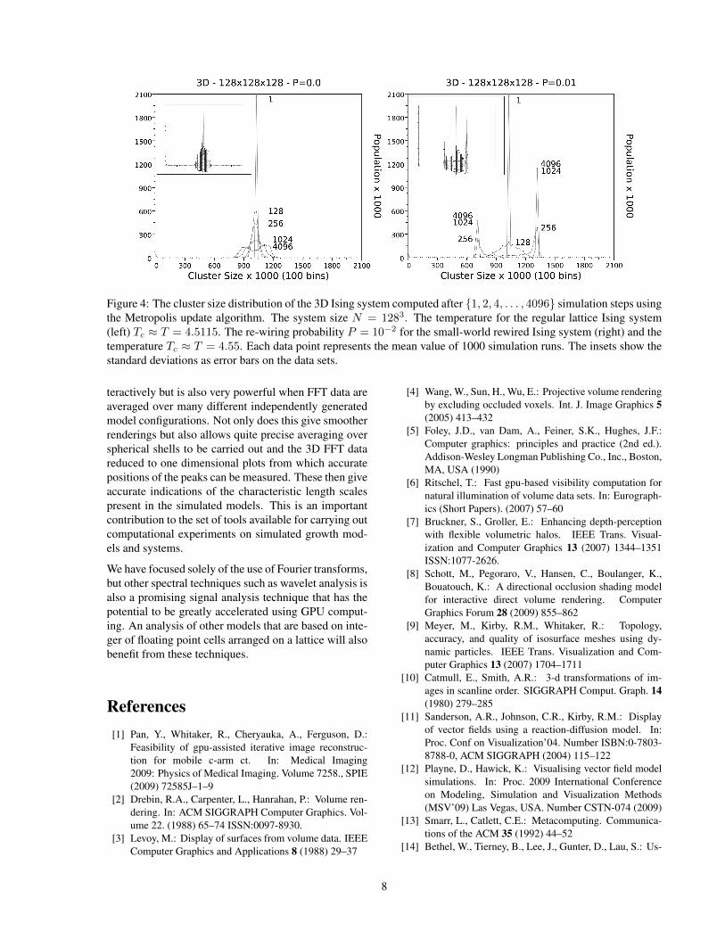
Figure 4: The cluster size distribution of the 3D Ising system computed after 1, 2, 4, . . . , 4096 simulation steps usingthe Metropolis update algorithm. The system size N = 1283. The temperature for the regular lattice Ising system(left) Tc ≈ T = 4.5115. The re-wiring probability P = 10−2 for the small-world rewired Ising system (right) and thetemperature Tc ≈ T = 4.55. Each data point represents the mean value of 1000 simulation runs. The insets show thestandard deviations as error bars on the data sets.

teractively but is also very powerful when FFT data areaveraged over many different independently generatedmodel configurations. Not only does this give smootherrenderings but also allows quite precise averaging overspherical shells to be carried out and the 3D FFT datareduced to one dimensional plots from which accuratepositions of the peaks can be measured. These then giveaccurate indications of the characteristic length scalespresent in the simulated models. This is an importantcontribution to the set of tools available for carrying outcomputational experiments on simulated growth mod-els and systems.

We have focused solely of the use of Fourier transforms,but other spectral techniques such as wavelet analysis isalso a promising signal analysis technique that has thepotential to be greatly accelerated using GPU comput-ing. An analysis of other models that are based on inte-ger of floating point cells arranged on a lattice will alsobenefit from these techniques.

References[1] Pan, Y., Whitaker, R., Cheryauka, A., Ferguson, D.:

Feasibility of gpu-assisted iterative image reconstruc-tion for mobile c-arm ct. In: Medical Imaging2009: Physics of Medical Imaging. Volume 7258., SPIE(2009) 72585J–1–9

[2] Drebin, R.A., Carpenter, L., Hanrahan, P.: Volume ren-dering. In: ACM SIGGRAPH Computer Graphics. Vol-ume 22. (1988) 65–74 ISSN:0097-8930.

[3] Levoy, M.: Display of surfaces from volume data. IEEEComputer Graphics and Applications 8 (1988) 29–37

[4] Wang, W., Sun, H., Wu, E.: Projective volume renderingby excluding occluded voxels. Int. J. Image Graphics 5(2005) 413–432

[5] Foley, J.D., van Dam, A., Feiner, S.K., Hughes, J.F.:Computer graphics: principles and practice (2nd ed.).Addison-Wesley Longman Publishing Co., Inc., Boston,MA, USA (1990)

[6] Ritschel, T.: Fast gpu-based visibility computation fornatural illumination of volume data sets. In: Eurograph-ics (Short Papers). (2007) 57–60

[7] Bruckner, S., Groller, E.: Enhancing depth-perceptionwith flexible volumetric halos. IEEE Trans. Visual-ization and Computer Graphics 13 (2007) 1344–1351ISSN:1077-2626.

[8] Schott, M., Pegoraro, V., Hansen, C., Boulanger, K.,Bouatouch, K.: A directional occlusion shading modelfor interactive direct volume rendering. ComputerGraphics Forum 28 (2009) 855–862

[9] Meyer, M., Kirby, R.M., Whitaker, R.: Topology,accuracy, and quality of isosurface meshes using dy-namic particles. IEEE Trans. Visualization and Com-puter Graphics 13 (2007) 1704–1711

[10] Catmull, E., Smith, A.R.: 3-d transformations of im-ages in scanline order. SIGGRAPH Comput. Graph. 14(1980) 279–285

[11] Sanderson, A.R., Johnson, C.R., Kirby, R.M.: Displayof vector fields using a reaction-diffusion model. In:Proc. Conf on Visualization’04. Number ISBN:0-7803-8788-0, ACM SIGGRAPH (2004) 115–122

[12] Playne, D., Hawick, K.: Visualising vector field modelsimulations. In: Proc. 2009 International Conferenceon Modeling, Simulation and Visualization Methods(MSV’09) Las Vegas, USA. Number CSTN-074 (2009)

[13] Smarr, L., Catlett, C.E.: Metacomputing. Communica-tions of the ACM 35 (1992) 44–52

[14] Bethel, W., Tierney, B., Lee, J., Gunter, D., Lau, S.: Us-

8

ing high-speed wans and network data caches to enableremote and distributed visualization. In: Proceedingsof the 2000 ACM/IEEE conference on Supercomputing.Number ISBN:0-7803-9802-5 (2000) Article 28:1–23

[15] Ng, R., Mark, B., Ebert, D.: Real-time programmablevolume rendering (2009)

[16] Fletcher, P.A., Robertson, P.K.: Interactive shading forsurface and volume visualization on graphics worksta-tions. In: VIS ’93: Proceedings of the 4th conference onVisualization ’93, Washington, DC, USA, IEEE Com-puter Society (1993) 291–298

[17] Vezina, G., Fletcher, P.A., Robertson, P.K.: Volume ren-dering on the maspar mp-1. In: VVS ’92: Proceedingsof the 1992 workshop on Volume visualization, NewYork, NY, USA, ACM (1992) 3–8

[18] Goodnight, N., Woolley, C., Lewin, G., Luebke, D.,Humphreys, G.: A multigrid solver for boundary valueproblems using programmable graphics hardware. In:Proc. ACM SIGGRAPH/EUROGRAPHICS Conf. onGraphics Hardware. Number ISBN ISSN:1727-3471,San Diego, California, USA. (2003) 102–111

[19] Poupyrev, I., Weghorst, S., Billinghurst, M., Ichikawa,T.: A framework and testbed for studying manipulationtechniques for immersive vr. In: VRST ’97: Proceed-ings of the ACM symposium on Virtual reality softwareand technology, New York, NY, USA, ACM (1997) 21–28

[20] Sanderson, A.R., Meyer, M.D., Kirby, R.M., Johnson,C.R.: A framework for exploring numerical solutionsof advection-reaction-diffusion equations using a gpu-based approach. Computing and Visualization in Sci-ence 12 (2009) 155–170

[21] Rumpf, M., Strzodka, R.: Nonlinear diffusion in graph-ics hardware. In: Proceedings of EG/IEEE TCVG Sym-posium on Visualization (VisSym ’01). (2001) 75–84

[22] Bolz, J., Farmer, I., Grinspun, E., Schrooder, P.: Sparsematrix solvers on the gpu: conjugate gradients andmultigrid. ACM Trans. Graph. 22 (2003) 917–924

[23] Beyer, J.: GPU-based Multi-Volume Rendering ofComplex Data in Neuroscience and Neurosurgery. PhDthesis, Institute of Computer Graphics and Algorithms,Vienna University of Technology, Favoritenstrasse 9-11/186, A-1040 Vienna, Austria (2009)

[24] NVIDIA R© Corporation: CUDATM 3.1 ProgrammingGuide. (2010) Last accessed September 2010.

[25] Ising, E.: Beitrag zur Theorie des Ferromagnetismus.Zeitschrift fuer Physik 31 (1925) 253?258

[26] Hawick, K.A.: Domain Growth in Alloys. PhD thesis,Edinburgh University (1991)

[27] Hawick, K.A.: Spectral analysis of growth in spa-tial lotka-volterra models. In: Proc. IASTED Interna-tional Conference on Modelling and Simulation. Num-ber CSTN-092, Gabarone, Botswana (2010)

[28] Ciccariello, S., Goodisman, J., Brumberger, H.: Onthe porod law. Journal of Applied Crystallography 21(1988) 117–128

[29] Windsor, C.G.: An Introduction to Small Angle NeutronScattering. J. Appl. Cryst. 21 (1988) 582–588

[30] Leist, A., Playne, D., Hawick, K.: Interactive visuali-sation of spins and clusters in regular and small-world

Ising models with CUDA on GPUs. Journal of Compu-tational Science 1 (2010) 33–40

[31] Hawick, K.A., James, H.A.: Ising model scal-ing behaviour on z-preserving small-world networks.Technical Report arXiv.org Condensed Matter: cond-mat/0611763, Information and Mathematical Sciences,Massey University (2006)

[32] Lorensen, W.E., Cline, H.E.: Marching cubes: A highresolution 3d surface construction algorithm. ComputerGraphics 21 (1987) 163–169

[33] Reddaway, S.F.: DAP a Distributed Array Processor.In: Proceedings of the 1st annual symposium on Com-puter Architecture,(Gainesville, Florida), ACM Press,New York (1973) 61–65

[34] Wilding, N., Trew, A., Hawick, K., Pawley, G.: Scien-tific modeling with massively parallel SIMD computers.Proceedings of the IEEE 79 (1991) 574–585

[35] Vozina, G., Fletcher, P., Robertson, P.: Volume Render-ing on the (MasPar) (MP-1). In: Workshop on VolumeVisualisation, Boston, MA., USA. (1992) 3–8

[36] Fletcher, P.A.: Visualisation on a massively parallel su-percomputer: Regular mapping and handling of multi-dimensional data on simd architectures,. In: Proceed-ings of the Fourth Australian Supercomputer Confer-ence, Bond University Qld. (1991)

[37] Hillis, W.D.: The Connection Machine. MIT Press(1985)

[38] Leist, A., Playne, D., Hawick, K.: Exploiting Graphi-cal Processing Units for Data-Parallel Scientific Appli-cations. Concurrency and Computation: Practice andExperience 21 (2009) 2400–2437 CSTN-065.

[39] Hawick, K., Leist, A., Playne, D.: Regular Lattice andSmall-World Spin Model Simulations using CUDA andGPUs. Int. J. Parallel Prog. 39 (2011) 183–201

9