technical programme - Thermodynamics of Chemical, Biological and

Hasija 1

EVALUATION OF STATISTICAL METHODS FOR GENERATING INJURY RISK CURVES Vikas Hasija Bowhead Systems Management, Inc Erik G. Takhounts Stephen A. Ridella NHTSA United States Paper Number: 11-0331 ABSTRACT

Statistical methods such as survival analysis (parametric and non-parametric) and logistic regression, along with other non-parametric methods such as Consistent Threshold Estimate and Certainty method are used for generating injury risk curves from biomechanical data. Recently, much attention has been drawn to the question of which statistical methodology is more appropriate in the construction of risk curves for biomechanical datasets. Most of the papers and reports focus on existing biomechanical datasets for which they generate various risk curves using parametric and non-parametric methods and then suggest the use of one method over another based on some sort of criteria. The purpose of this paper is to look at the same statistical methods, but from the “inverse perspective”, e.g. evaluate different statistical methods using non-correlated, randomly generated data and to see if any of the widely used methods would yield a “good” risk curve when they are supposed to yield a “bad” risk curve. The “goodness” of a risk curve was evaluated based on 95% confidence intervals, the shape of the curve, and “goodness of fit” statistics. If the risk curve had a well pronounced S-shape, narrow confidence intervals and good “goodness of fit” statistics, then the method was concluded to be inappropriate for non-correlated datasets as it was expected to yield poor S-shape, wide confidence intervals and poor “goodness of fit” statistics. A well-correlated, randomly generated dataset was also evaluated using the various statistical methods. It was observed that logistic regression was able to clearly identify both the non-correlated and well-correlated datasets but suffered because of the underlying distribution that sometimes resulted in non-zero injury probability at zero stimulus level. Survival analysis with different types of censoring and underlying distributions was closely studied. Survival Analysis with a Weibull/ Log-Logistic/ Log-Normal underlying distribution and left- right censored data was not only able to clearly identify both non-correlated and well-correlated datasets, but also gave zero injury probability at zero stimulus level. This paper presents a new perspective of judging the applicability of the

various statistical methods and recommends the statistical method, censoring technique, and the distributions that may be used for generating injury risk curves from biomechanical datasets. INTRODUCTION Injury risk curves are developed by statistically analyzing experimental data (human and/or animal data) to find an injury criterion and then developing a relationship between this criterion and the type of injury (Kuppa et al [1]). In essence, injury risk curves define the probability of injury to a certain body region as a function of a predictor variable like force, deflection etc. Injury risk curves are used to establish Injury Assessment Reference Values (IARV) (Eppinger et al [2], Mertz et al [3]) that are used for assessing occupant injuries in crash tests. Depending on the IARV’s, a car can get an acceptable, good, or poor rating. Thus the importance of correctly generating the injury risk curves cannot be overstated. Various statistical methods such as survival analysis (parametric and non-parametric) and logistic regression, along with other non-parametric methods such as Consistent Threshold Estimate and Certainty method are used for generating injury risk curves from biomechanical data (Kuppa et al [1], Eppinger et al [2], Mertz et al [4], Petitjean et al [5], , McKay et al [6], Yoganandan et al [7], Kent et al [8], Banglmaier et al [9], Banglmaier et al [10], Nusholtz et al [11], Domenico [12], Wang et al [13], Domenico et al [14]). Much of attention has been drawn recently to the question of which statistical methodology is more appropriate in the construction of risk curves for biomechanical datasets (Petitjean et al [5], Kent et al [8], Nakahira et al [15]). Some of the papers generate various risk curves using parametric and non-parametric methods and then suggest the use of one method over another based on some criteria (e.g. McKay et al [6], Kent et al [8], Banglmaier et al [9], Nakahira et al [15], Domenico [12], and Wang et al [13]).

The method used for risk curve generation should be properly evaluated. For example McKay et

Hasija 2

al [6] obtained uncensored data from their experiments using acoustic sensors and generated a tibia axial force injury risk curve using survival analysis with uncensored/right censored technique assuming logistic distribution. A “good” risk curve was generated using survival analysis even when most of the injury points were to the left of the non-injury points (McKay et al [6], Figure 14, Page 243). Also their risk curve had non-zero injury probability at zero tibia axial force. Since McKay et al [6] assumed logistic distribution, they obtained non-zero injury probability at zero stimulus. For datasets such as McKay’s, other variables and confounding factors should be considered. Such datasets indicate that more testing needs to be done to add more points to the dataset before generating the risk curve. Instead McKay et al [6] have generated a “good” risk curve using uncensored survival analysis. Also Kent at el [8] studied the different data censoring schemes and distributions for injury risk curve generation. They concluded that uncensored/right censored survival analysis is an appropriate method for generating risk curves when logistic regression and left/right censored survival analysis are not able to generate a relevant risk curve. This paper evaluates uncensored survival analysis with various distributions, in addition to other statistical methods, to assess the usefulness of this technique. Wang et al [13] concludes that interval censored injury data (when an observation is an injury, it is treated as interval censored from zero to the observed stimulus value instead of left censored where injury could occur anywhere from –∞ to observed stimulus value) improves the risk curve generation. In their study, one of the methods used was survival analysis with normal distribution and interval censoring as mentioned above. This paper also evaluates interval censored survival analysis with normal distribution to assess its effectiveness for risk curve generation. This paper evaluates statistical methods based on an “inverse perspective” where non-correlated datasets are used for evaluation purposes. Based on the results of non-correlated datasets, further study is carried out on well-correlated dataset and appropriate statistical methods are identified that may be used to generate injury risk curves.

METHODOLOGY Prior to describing the methodology, a few definitions used in this paper are given below:

a. Correlation: Relationship between independent (X) and dependent variable (Y). Correlation is computed using R2, Pearson correlation coefficient, Point Biserial

correlation coefficient and the p-value. A p-value of > 0.05 was defined to have no statistically significant correlation.

b. Non-correlated dataset: The independent and dependent variables have no or very poor correlation as determined by R2, Pearson correlation coefficient, Point Biserial correlation coefficient and the p-value

c. Well-correlated dataset: The independent and dependent variables have strong correlation as determined by R2 , Pearson correlation coefficient, Point Biserial correlation coefficient and the p-value

d. Point (0, 0): indicates zero injury probability at zero stimulus level.

e. “Goodness of Fit” for Logistic Regression*: is tested using Receiver Operating Characteristic (ROC) curve, Hosmer-Lemeshow statistic [16], and “Max Loglikelihood”. Greater area under the ROC curve, lower value of Hosmer-Lemeshow statistic and lower value of “Max Loglikelihood” indicate better fit to data. A ROC plot shows the false positive rate (1-specificity) on the X axis and the true positive rate (sensitivity or 1 - the false negative rate) on the Y axis. The accuracy of a test is measured by the area under the ROC curve. The closer the curve follows the left-hand border and then the top border of the ROC space, the more accurate the test; the true positive rate is high and the false positive rate is low. Statistically, more area under the curve means that it is identifying more true positives while minimizing the number/percent of false positives.

f. “Goodness of Fit” for Survival Analysis*: is computed using “Max Loglikelihood”. Lower value of “Max Loglikelihood” indicates better fit. * The “goodness of fit” statistics described above can only be compared for different models on the same dataset and not across datasets.

g. “Good” risk curve: Good S-shape curve, narrow 95% confidence intervals, and good “goodness of fit” statistics.

h. “Bad” risk curve: Poor S-shape curve or near flat/flat curve, wide 95% confidence intervals, and poor “goodness of fit” statistics. *Shape of the risk curve is purely a qualitative factor.

i. Left censored: An injury point (x, 1) is defined as left censored when the injury threshold lies in the interval [-∞ , x].

Hasija 3

j. Right censored: A non-injury point (x, 0) is defined as right censored when the injury threshold lies in the interval [x, ∞+ ].

k. Interval censored: An injury point (x, 1) is defined as interval censored when the injury threshold lies in the interval [k, x], where k is the point when subject is uninjured and x is a point when subject is injured.

l. Uncensored: An injury point (x, 1) is defined as uncensored when the injury threshold is equal to x.

The methodology for evaluating various statistical methods is shown in Figure 1. Figure 1. Methodology flow chart Both the non-correlated datasets and the well-correlated dataset are considered for the purpose of evaluation. For the non-correlated datasets, various statistical methods mentioned in Table 1 are used to generate risk curves. In addition to the four distributions i.e. Weibull, Normal, Logistic and Log-Normal commonly used for biomechanics risk function (Kent et al [8], Banglmaier et al [9], Banglmaier et al [10], Wang et al [13]), other distributions were also studied (Table 1). It is also observed that risk curves are generated using survival analysis with Normal distribution where injury data is interval censored [0, failure] (Banglmaier et al [9], Banglmaier et al [10], and Wang et al [13]). This special case of interval censoring was also studied.

Table 1. Statistical methods used for Non-correlated

datasets Method Distribution Injury Non-

Injury Survival Analysis

Non-parametric

Uncensored Right censored

Survival Analysis

Normal Uncensored Right censored

Survival Analysis

Normal Left censored

Right censored

Survival Analysis

Weibull Left censored

Right censored

Survival Analysis

Weibull Uncensored Right censored

Survival Analysis

Log-Logistic Uncensored Right censored

Survival Analysis

Log-Logistic Left censored

Right censored

Survival Analysis

Log-Normal Left censored

Right censored

Survival Analysis

Log-Normal Uncensored Right censored

Survival Analysis

Logistic Left censored

Right censored

Survival Analysis

Logistic Uncensored Right censored

Survival Analysis

Extreme Value

Left censored

Right censored

Survival Analysis

Extreme Value

Uncensored Right censored

Survival Analysis

Normal

Interval Censored

Right censored

Other Methods Logistic Regression

Consistent Threshold Estimate Method Certainty Method

The various distributions mentioned in Table1 are shown in Figures 2-6.

(1). Figure 2. Normal Distribution

No

No

Well-Correlated Dataset

Yes

Appropriate Statistical Method to Use for Generating Injury Risk Curve

Various Statistical Methods

Non-Correlated Datasets

Reject Statistical Method

Yes

“Bad” risk curve?

“Good” risk curve

+ Point (0,0)?

Hasija 4

(2). Figure 3. Logistic Distribution

(3). Figure 4: Log-Normal Distribution

(4). Figure 5: Weibull Distribution

(5). Figure 6: Extreme Value Distribution First, the statistical methods as listed in Table 1 are used for generating injury risk curves for non-correlated datasets. For non-correlated datasets, the shape of the risk curve, the 95% confidence intervals and “goodness of fit” statistics are checked for each statistical method. If the risk curve looks “good”, the corresponding statistical method is rejected as it should have generated a “bad” risk curve for the non-correlated dataset. Second, analysis is carried out to test the applicability of survival analysis with uncensored data for risk curve generation. It is our understanding that survival analysis with uncensored data has an effect of adding extra points to the analysis. To show this, two examples are presented (1) how uncensored analysis works by adding extra points (example 1) and (2) how as few as two injury data points and no non-injury points are enough to generate a good S-shape risk curve using uncensored survival analysis (example 2).

Finally, the statistical methods that pass the non-correlated dataset are used for generating injury risk curves for the well-correlated dataset. For the well-correlated dataset, the shape of the risk curves, 95% confidence intervals, “goodness of fit” statistics and the injury probability at zero stimulus level are considered. The statistical methods that satisfy the conditions of a “good” risk curve and point (0, 0) are accepted and identified as appropriate methods that may be used for generating injury risk curves from biomechanical data. Datasets Three datasets were used for evaluation purposes: Dataset 1 and Dataset 2 (Non-Correlated) The first dataset was obtained from the cadaver tests conducted by University of Virginia, where the number of rib fractures was used as a dependent

Hasija 5

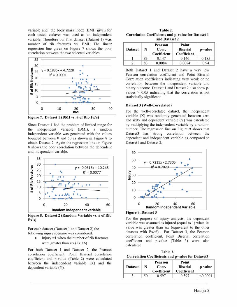
variable and the body mass index (BMI) given for each tested cadaver was used as an independent variable. Therefore our first dataset (Dataset 1) was number of rib fractures vs. BMI. The linear regression line given on Figure 7 shows the poor correlation between the two selected variables.

Figure 7. Dataset 1 (BMI vs. # of Rib Fx’s)

Since Dataset 1 had the problem of limited range for the independent variable (BMI), a random independent variable was generated with the values bounded between 0 and 50 as shown in Figure 8 to obtain Dataset 2. Again the regression line on Figure 8 shows the poor correlation between the dependent and independent variable.

Figure 8. Dataset 2 (Random Variable vs. # of Rib Fx’s) For each dataset (Dataset 1 and Dataset 2) the following injury scenario was considered:

• Injury =1 when the number of rib fractures were greater than six (Fx >6).

For both Dataset 1 and Dataset 2, the Pearson correlation coefficient, Point Biserial correlation coefficient and p-value (Table 2) were calculated between the independent variable (X) and the dependent variable (Y).

Table 2. Correlation Coefficients and p-value for Dataset 1

and Dataset 2

Dataset

N Pearson

Corr. Coefficient

Point Biserial

Coefficient

p-value

1 83 0.147 0.146 0.185 2 83 0.0084 0.0084 0.94

Both Dataset 1 and Dataset 2 have a very low Pearson correlation coefficient and Point Biserial Correlation coefficients indicating very weak or no correlation between the independent variable and binary outcome. Dataset 1 and Dataset 2 also show p-values > 0.05 indicating that the correlation is not statistically significant.

Dataset 3 (Well-Correlated) For the well–correlated dataset, the independent variable (X) was randomly generated between zero and sixty and dependent variable (Y) was calculated by multiplying the independent variable by a random number. The regression line on Figure 9 shows that Dataset3 has strong correlation between the dependent and independent variable as compared to Dataset1 and Dataset 2.

Figure 9. Dataset 3 For the purpose of injury analysis, the dependent variable was assumed as injured (equal to 1) when its value was greater than six (equivalent to the other datasets with Fx>6). For Dataset 3, the Pearson correlation coefficient, Point Biserial correlation coefficient and p-value (Table 3) were also calculated.

Table 3. Correlation Coefficients and p-value for Dataset3

Dataset

N

Pearson Corr.

Coefficient

Point Biserial

Coefficient

p-value

3 50 0.597 0.597 <0.0001

y = 0.1835x + 4.7228R² = 0.0091

0

5

10

15

20

25

30

35

0 10 20 30 40

# of

Rib

frac

ture

s

BMI

y = -0.0616x + 10.245R² = 0.0077

0

5

10

15

20

25

30

35

0 20 40 60

# of

Rib

Fra

ctur

es

Random Independent variable

y = 0.7215x - 2.7305R² = 0.7029

0

10

20

30

40

50

60

0 20 40 60

Inju

ry

Random Independent Variable

Hasija 6

Dataset 3 shows relatively high Pearson correlation coefficient and Point Biserial correlation coefficient as compared to Dataset 1 and Dataset2 indicating moderate to reasonably strong correlation between the independent variable and binary outcome. Also, Dataset 3 shows p-value of < 0.0001 indicating that the correlation is statistically significant. Break-Down Data for Example 1 For evaluating example 1, Dataset 3 was used to generate Break-Down data as follows:

• Injury data is uncensored i.e. it is exactly known at what stimulus the sample breaks. So, for each injury point, ten extra injury points are added to the right of the corresponding data point and ten extra non-injury points are added to the left of the corresponding data point as shown in Table 4 (original point in red).

Table 4. Break-Down data

1 60 1 57.4 1 54.8 1 52.2 1 49.6 1 47 1 44.4 1 41.8 1 39.2 1 36.6 1 34 0 30.6 0 27.2 0 23.8 0 20.4 0 17 0 13.6 0 10.2 0 6.8 0 3.4 0 0

• For each non-injury point, ten additional non-injury points are added to the left of the corresponding data point as shown in Table 5 (original point in red).

Table 5. Break-Down of data

0 15

0 13.5 0 12 0 10.5 0 9 0 7.5 0 6 0 4.5 0 3 0 1.5 0 0

A program was written to add extra points to the dataset. The interval at which additional injury points were added is given by Equation 6.

1060 stimulus− (6).

where 60 represents the maximum stimulus. The interval at which additional non-injury points were added is given by Equation 7.

100−stimulus (7).

where 0 represents the minimum stimulus. Break-Down of Dataset 3 in this manner led to a total of 900 data points from 50 points.Statistical analysis was conducted on Dataset 3 (original data) and Break-Down data as shown in Table 6.

Table 6. Statistical Methods used for Break-Down Data

Methods

Survival analysis on original data with normal distribution + uncensored injury points and right censored non-injury points.

Logistic regression on Original data

Logistic regression on Break-Down data.

Dataset for Example 2

For evaluating example 2, a hypothetical dataset (Table 7) was generated where three different laboratories test a sample and come up with their set of injury points

Table 7. Injury points

Lab Injury Stimulus Value

Hasija 7

Lab1- Set1 1 40 1 45

Lab2-Set 2 1 35 1 40

Lab3-Set 3 1 45 1 50

Uncensored survival analysis is studied with this dataset (Table 7) SAS [17] was used to run the statistical analysis. The PROC RELIABILITY procedure in SAS was used to run survival analysis with different data censoring schemes and with various distributions as listed in Table 1. PROC LOGISTIC was used to run logistic regression and generate ROC curves. Non-parametric Survival analysis was carried out in SAS using PROC LIFETEST Apart from the statistical methods mentioned in Table 1; other non-parametric methods i.e. Certainty method and Consistent Threshold Estimate method were also used for risk curve generation. These methods were programmed in Visual Basic and interfaced with MS Excel. RESULTS Dataset1: This dataset was evaluated using all statistical methods (Table 1) and showed a similar trend as Dataset 2. For more clarity, all results are presented for Dataset 2 but only the injury risk curves generated using Certainty and CTE methods are shown for Dataset 1. Figure 10 and Figure 11 show the injury risk curves obtained using the Certainty and Consistent Threshold Estimate (CTE) methods respectively.

Figure 10. Certainty method

Figure 11. CTE method Dataset 2: Figures 12-27 show the injury risk curves for dataset 2 using statistical methods mentioned in Table1.

Figure 12. Certainty method

Figure 13. CTE method

00.10.20.30.40.50.60.70.80.9

1

10.0 15.0 20.0 25.0 30.0 35.0

Prob

abili

ty o

f Inj

ury

BMI

Test Data

Certainity Method

00.10.20.30.40.50.60.70.80.9

11.1

0.0 10.0 20.0 30.0 40.0

Prob

abili

ty o

f Inj

ury

BMI

CTE

Test Data

00.10.20.30.40.50.60.70.80.9

1

0 20 40 60

Prob

abili

ty o

f Inj

ury


Injury Data

Certainity Method

00.10.20.30.40.50.60.70.80.9

1

0 20 40 60

Prob

abili

ty o

f Inj

ury


CTE Method

Injury Data

Hasija 8

Figure 14. Logistic regression and non-parametric survival analysis

Figure 15. Logistic regression and survival analysis (Left/Right censoring +Normal Distribution)

Figure 16. Logistic regression and survival analysis (Uncensored/Right Censored +Normal Distribution)

Figure 17. Logistic regression and survival analysis (Left/Right censoring +Log-Normal Distribution)

Figure 18. Logistic regression and survival analysis (Uncensored/Right Censored + Log-Normal Distribution)

Figure 19. Logistic regression and survival analysis (Left/Right Censoring +Weibull Distribution)

0

0.2

0.4

0.6

0.8

1

0 20 40 60

Prob

abili

ty o

f In

jury


SurvivalLogistic95% CIInjury data

00.10.20.30.40.50.60.70.80.9

1

0 20 40 60

Prob

abili

ty o

f Inj

ury


Logistic95% CISurvival95% CIInjury Data

0

0.2

0.4

0.6

0.8

1

0 20 40 60

Prob

abili

ty o

f Inj

ury



0

0.2

0.4

0.6

0.8

1

0 20 40 60

Prob

abili

ty o

f Inj

ury


Logistic95% CISurvival95% CIInjury data

0

0.2

0.4

0.6

0.8

1

0 20 40 60

Prob

abili

ty o

f Inj

ury



0

0.2

0.4

0.6

0.8

1

0 20 40 60

Prob

abili

ty o

f Inj

ury



Hasija 9

Figure 20. Logistic regression and survival analysis (Uncensored/Right Censored +Weibull Distribution)

Figure 21. Logistic regression and survival analysis (Left/Right Censoring +Logistic Distribution)

Figure 22. Logistic regression and survival analysis (Uncensored/Right Censored +Logistic Distribution)

Figure 23. Logistic regression and survival analysis (Left/Right Censoring +Log-Logistic Distribution)

Figure 24. Logistic regression and survival analysis (Uncensored/Right Censored + Log-Logistic Distribution)

Figure 25. Logistic regression and survival analysis (Left/Right Censoring +Extreme Value Distribution)

0

0.2

0.4

0.6

0.8

1

0 20 40 60

Prob

abili

ty o

f Inj

ury



0

0.2

0.4

0.6

0.8

1

0 20 40 60

Prob

abili

ty o

f Inj

ury



0

0.2

0.4

0.6

0.8

1

0 20 40 60

Prob

abili

ty o

f Inj

ury


Logisitc95% CISurvival95% CIInjury Data

0

0.2

0.4

0.6

0.8

1

0 20 40 60

Prob

abili

ty o

f Inj

ury



0

0.2

0.4

0.6

0.8

1

0 20 40 60

Prob

abili

ty o

f Inj

ury



0

0.2

0.4

0.6

0.8

1

0 20 40 60

Prob

abili

ty o

f Inj

ury



Hasija 10

Figure 26. Logistic regression and survival analysis (Uncensored/Right Censored + Extreme Value Distribution)

Figure 27. Logistic regression and Survival analysis (Interval Censored /Right Censored + Normal distribution) Figure 28, Table 8 and Table 9 show the fit statistics for logistic regression and survival analysis corresponding to Figures 14-27.

Figure 28. ROC Curve for Dataset 2.

Table 8. Fit Statistics for Dataset 2 (Logistic Regression)

Logistic Regression (Figures 14-27)

Hosmer-Lemeshow

Goodness-of-Fit

Max Loglikelihood

7.27 -56.797

Table 9.

Fit Statistics for Dataset 2 (Survival Analysis)

Survival Analysis Max Loglikelihood

Figure 15 Normal +LC/RC -56.79 Figure 16 Normal + UC/RC -203.76 Figure 17 Log-Normal +LC/RC -56.78 Figure 18 Log-Normal +UC/RC -73.38 Figure 19 Weibull +LC/RC -56.78 Figure 20 Weibull +UC/RC -69.25 Figure 21 Logistic +LC/RC -56.79 Figure 22 Logistic +UC/RC -204.57 Figure 23 Log-logistic +LC/RC -56.78 Figure 24 Log-logistic +UC/RC -70.5 Figure 25 Extreme Value +LC/RC -56.79 Figure 26 Extreme Value +UC/RC -212.12 Figure 27 Normal +IC/RC -84.85 Based on the results of non-correlated datasets, the uncensored/right censoring scheme was eliminated from contention for risk curve generation as the uncensored analysis generates “good” risk curves even for non-correlated data (Figures 16, 18, 20, 22, 24 and 26). The interval censoring scheme (with injury interval defined from [0, failure]) with normal distribution also was not considered for further study for the same reason (Figure 27). Example 1: The results obtained using statistical methods (Table 6) on original data (Dataset 3) and Break-Down data are shown in Figure 29. It can be seen that logistic regression on Break-Down data converges to survival analysis on original data i.e. analyzing data using survival analysis with uncensored injury points and right censored non-injury points is equivalent to logistic regression with additional points manually added. This example shows that uncensored analysis has the effect of adding more points to the analysis and therefore changes the distribution of the original population.

0

0.2

0.4

0.6

0.8

1

0 20 40 60

Prob

abili

ty o

f In

jury



0

0.2

0.4

0.6

0.8

1

0 20 40 60

Prob

abili

ty o

f Inj

ury



0

0.2

0.4

0.6

0.8

1

0 0.5 1

Sens

itiv

ity

1-Specificity

ROC Curve

Area under curve=0.5

Hasija 11

Figure 29. Statistical analysis on Original and Break-Down data. Example 2: As shown in example 1, uncensored analysis has the effect of adding extra points to the analysis. Thus uncensored analysis allows for risk curve generation based on just two injury points and no non-injury points. As a result each laboratory can come up with its own risk curve as shown in Figure 30.

Figure 30. Risk curves using two injury points

Dataset3: Based on the results of non-correlated datasets (Dataset1 & Dataset 2) and the uncensored survival analysis examples, Dataset 3 was studied in detail using only logistic regression and left / right censored survival analysis with various distributions. For completeness, Dataset3 was evaluated using uncensored survival analysis with Weibull distribution only and non-parametric survival analysis. The injury risk curves generated for Dataset3 are shown in Figures 31-37.

Figure 31. Logistic regression and survival analysis (Left/Right censored + Normal Distribution)

Figure 32. Logistic regression and survival analysis (Left/Right censored + Log-Normal Distribution)

Figure 33. Logistic regression and survival analysis (Left/Right censored + Logistic Distribution)

0

0.2

0.4

0.6

0.8

1

0 20 40 60

Prob

abili

ty o

f Inj

ury


Logistic on Org DataSurvival on Original DataLogistic-Breakdown

0

0.2

0.4

0.6

0.8

1

0 20 40 60

Prob

abili

ty o

f Inj

ury


Survival-Set 1Survival-Set 2Survival-Set 3Injury Set 1Injury Set 2Injury Set 3

0

0.2

0.4

0.6

0.8

1

0 20 40 60

Prob

abili

ty o

f Inj

ury



0

0.2

0.4

0.6

0.8

1

0 20 40 60

Prob

abili

ty o

f Inj

ury



0

0.2

0.4

0.6

0.8

1

0 20 40 60

Prob

abili

ty o

f Inj

ury


Logistic

95% CI

Survival

95% CI

Injury data

Hasija 12

Figure 34. Logistic regression and survival analysis (Left/Right censored + Log-Logistic Distribution)

Figure 35. Logistic regression and survival analysis (Left/Right censored + Weibull Distribution)

Figure 36. Logistic regression and survival analysis (Left/Right censored + Extreme Value Distribution)

Figure 37. Logistic regression, survival analysis (Uncensored/Right censored + Weibull Distribution) and non-parametric survival analysis. Figure 38, Table 10 and Table 11 show the fit statistics for logistic regression and survival analysis corresponding to Figures 31-37.

Figure 38. ROC Curve for Dataset 3

Table 10.

Fit Statistics for Dataset 3 (Logistic Regression)

Logistic Regression (Figures 14-27)

Hosmer-Lemeshow

Goodness-of-Fit

Max Loglikelihood

3.35 -16.563

Table 11.

Fit Statistics for Dataset 3 (Survival Analysis)

Survival Analysis Max Loglikelihood

Figure 31 Normal +LC/RC -16.61 Figure 32 Log-Normal +LC/RC -15.84

0

0.2

0.4

0.6

0.8

1

0 20 40 60

Prob

abili

ty o

f Inj

ury


Logistic95% CI

Survival95% CI

Injury Data

0

0.2

0.4

0.6

0.8

1

0 20 40 60

Prob

abili

ty o

f Inj

ury


Logistic

95% CI

Survival

95% CI

Injury Data

00.10.20.30.40.50.60.70.80.9

1

0 20 40 60

Prob

abili

ty o

f Inj

ury


Logistic

95% CI

Survival

95% CI

Injury Data

0

0.2

0.4

0.6

0.8

1

0 20 40 60

Prob

abili

ty o

f Inj

ury


Survival-NPLogistic95% CISurvival-UC/RC95% CIInjury Data

0

0.2

0.4

0.6

0.8

1

0 0.5 1

Sens

itiv

ity

1-Specificity

ROC Curve for Well-correlated dataset

Area under curve=0.91

Hasija 13

Figure 33 Logistic +LC/RC -16.56 Figure 34 Log-logistic +LC/RC -16.01 Figure 35 Weibull +LC/RC -16.13 Figure 36 Extreme Value +LC/RC -17.38 Figure 37 Weibull +UC/RC -27.69 Based on the study, it was found that survival analysis with left/right data censoring scheme and with Weibull or Log-Normal or Log-Logistic distribution satisfied the conditions of a “good” risk curve and point (0, 0). The corresponding risk curves are plotted and compared with logistic regression risk curve (Figure 39).

Figure 39. Logistic regression and survival analysis (Left/Right censored + Log-Normal Distribution, Left/Right censored + Log-Logistic Distribution, Left/Right censored + Weibull Distribution) DISCUSSION

This study was conducted to analyze various statistical methods using non-correlated and well-correlated datasets. It is observed that certain statistical methods generate “good” risk curves even when the underlying data is non-correlated as is evidenced by the Figures 10 through 27.

These methods are: 1) Non-parametric survival analysis with uncensored injury data and censored non-injury data (Figure 14); 2) Parametric survival analysis with uncensored injury data and right censored non-injury data with any assumed underlying distribution (Figures 16, 18, 20, 22, 24 and 26); 3) Survival analysis with normal distribution when injury data is interval censored [0, failure] and non-injury data is right censored (Figure 27); and 4) Certainty method and Consistent Threshold method (Figures 10, 11, 12 and 13).

Once data is arranged in ascending order, CTE method computes probability of injury subject to the constraint that the risk of injury at any given

stimulus is greater than or equal to the risk at the preceding stimulus. Thus CTE method cannot differentiate between the non-correlated and the well-correlated datasets and always generates an injury risk curve where probability of injury increases over the range of the stimulus (Figures 11 and 13). In addition, the CTE method, just like any other non-parametric method depends on the sample that may not be representative of a population under consideration.

It is observed that logistic regression along with the survival analyses with Normal /Weibull /EVD /Logistic /Log- Logistic /Log-Normal distributions when injury data is left censored and non-injury data is right censored yielded better differentiation of the non-correlated data (Figures 15, 17, 19, 21, 23 and 25). Kent et al [8] suggests that treating the uncensored data as censored data can result in an incorrect risk curve and may in fact suggest no correlation or inverse correlation between injury and a parameter that is actually an accurate predictor of injury. However, it is observed from Figures 16, 18, 20, 22, 24 and 26 that survival analysis with uncensored injury data can generate a “good” risk curve even for the non-correlated dataset whereas left /right censored survival analysis (Figures 15, 17, 19, 21, 23 and 25) is able to capture the poor correlation between the independent and dependent variable appropriately by generating a “bad” risk curve. The Pearson correlation coefficient, Point Biserial correlation coefficient and p-value were computed for two datasets that are used in Kent et al [8] study. These are Banglmaier dataset (Banglmaier et al [18], Banglmaier et al [19]) and Klopp dataset (Klopp et al [20]). Banglmaier dataset (Kent et al [8]) has a Pearson correlation coefficient and Point Biserial correlation coefficient of 0.204 with a p-value of 0.2324 and Klopp dataset (Kent et al [8]) has a Pearson correlation coefficient and Point Biserial correlation coefficient of 0.0044 with a p-value of 0.9758 which indicates poor correlation between the independent and dependent variable. Thus it is observed that in Kent et al [8] study, doubly (left/right) censored survival analysis and logistic regression is able to capture the trend (poor correlation) properly as compared to uncensored survival analysis that generates a “good” risk curve for non-correlated data (Kent et al [8]- Figure 10 and Figure 12). Thus, the ability of uncensored analysis and the inability of censored analysis to generate a “good” risk curve may not necessarily imply that the risk curve generated by uncensored analysis is correct. All it may mean is that the dataset has poor correlation or requires further investigation to find any confounding factors or may require additional tests to add more data points. Kent et al [8] mentions

0

0.2

0.4

0.6

0.8

1

0 20 40 60

Prob

abili

ty o

f inj

ury


Log Normal 95% CILog Logistic95% CIWeibull 95% CILogistic

Hasija 14

that it is not necessary to perform non-injury tests when using uncensored analysis for risk curve generation. In our study, from Example 1 and Example 2, it is observed that uncensored analysis has an effect of adding extra points to the analysis (Figure 29), which helps create a good S-shape risk curve with just two injury points and no non-injury points (Figure 30). However, these risk curves may be misleading as the effect of adding extra points changes the underlying population.

From the study of the well-correlated dataset, several observations can be made based on Figures 31 – 37 and Figure 39.

First, uncensored survival analysis gives the best fit for the well-correlated dataset (Figure 37 and Table 11) but we already observed that survival analyses with uncensored injury data generates “good” risk curves even for the non-correlated dataset (Figures 16, 18, 20, 22, 24 and 26). Without this knowledge Figure 37 may be misleading.

Second, logistic regression and survival analysis with normal/logistic distribution when injury data is left censored and non-injury data is right censored, yield similar results (Figures 31 and 33).

Third, survival analysis with Extreme value distribution (EVD) when injury data is left censored and non-injury data is right censored results in a risk curve which differs from logistic regression risk curve in the 0%-30% probability range after which both risk curves are similar (Figure 36). Both the risk curves do not pass through point (0, 0). Finally, survival analysis with Weibull/ Log-Normal/ Log-Logistic distribution when injury data is left censored and non-injury data is right censored resulted in risk curves very similar to that of logistic regression with the exception of the fact that they pass through the point (0,0) (Figures 32, 34 and 35). Because of this the logistic regression and survival risk curves differ in the 0%-18% probability range after which they are very similar. Thus the two analyses i.e. survival analysis (with left censored injury data and right censored non-injury data) and logistic regression yield almost similar results for both the non-correlated and the well-correlated datasets. In addition, survival analysis with Weibull/ Lognormal/ Log-Logistic distribution offers a physically meaningful advantage of passing through point (0, 0). Nakahira et al [15] also suggests “zero predicted risk for no applied stimulus” as an assumption for accuracy of risk curve. Since crash performance is evaluated in the lower regions of the risk curve (Banglmaier et al [10]), using left/right censored survival analysis with either Weibull or Log-normal or Log-Logistic distribution for risk curve generation may be more suitable than logistic regression. However, an alternate approach may be to use a

combination of logistic regression and survival analysis. As compared to survival analysis, logistic regression provides additional fit statistics which may be useful to determine which covariates or combination of covariates best predict the dependent variable. Thus a combination of logistic regression analysis to determine the best predictive model followed by left/right censored survival analysis using Weibull or Log-normal or Log-Logistic distribution forcing the risk curve through zero may be an alternate approach.

Weibull, Log-normal and Log-logistic distributions offer this meaningful advantage of passing through point (0, 0) because these distributions range from 0 to +∞ (Figure 4 and 5). These distributions show very similar results including 95% CI and “goodness of fit” statistics (Figure 39 and Table 11) and thus the distribution of choice from among them can be based on some sort of fit statistics like Max Loglikelihood, Akaike’s Information Criterion (AIC) etc.

It is important to point out that all the datasets (Dataset 1, Dataset 2, and Dataset 3) evaluated in this paper have a sample size greater than or equal to 50. Since many biomechanical studies may have smaller sample size (12-15 data points), the observations made in this paper may or may not extrapolate to smaller datasets.

CONCLUSION 1. This study showed that the following statistical

methods do not yield better differentiation between well-correlated and non-correlated datasets:

a. Survival analysis with the data assumed to be normally distributed when injury data is interval censored, and non-injury data is right censored

b. Survival Analysis with any distribution when injury data is uncensored and non-injury data is right censored

c. Non-parametric survival analysis with uncensored injury data and censored non-injury data.

d. Consistent threshold method and Certainty method

2. Logistic regression and survival analysis with any distribution when injury data is left censored and non-injury data is right censored were able to differentiate better between non-correlated and well-correlated datasets.

3. Survival analysis with Weibull or log-logistic or log-normal distribution when injury data is left censored and non-injury data is right censored offers a physically meaningful advantage (in comparison with logistic regression) of passing

Hasija 15

through (0,0) point, i.e. has zero probability of injury at zero stimulus. This may be important when low probabilities of injuries are intended.

4. A combination of logistic regression and left/right censored survival analysis may be used as an alternate approach.

REFERENCES [1] Kuppa, S., Wang, J., Haffner, M., Eppinger, R., 2001 “ Lower Extremity Injuries and Associated Injury Criteria”, 17th ESV Conference. Paper No. 457. [2] Eppinger, E., Sun, E., Bandak, F., Haffner, M., Khaewpong, N., Maltese, M., Nguyen, T., Takhounts, E.G., Tannous, R., Zhang, A., Saul, R., 1999 “Development of Improved Injury Criteria for the Assessment of Advanced Automotive Restraint Systems – II.” NHTSA Report. [3] Mertz, H.J., Irwin, A.L., Prasad, P., 2003. “Biomechanical and Scaling Bases for Frontal and Side Impact Injury Assessment Reference Values.” Stapp Car Crash Journal, Vol. 47: 155-188. [4] Mertz, H.J., Prasad, P., Nusholtz, G., 1996. “Head Injury Risk Assessment for Forehead Impacts” SAE Technical Paper Series, 960099. [5] Petitjean, A., Trosseille, X., Petit, P., Irwin, A., Hassan, J., Praxl, N., 2009. “Injury Risk Curves for the WorldSID 50th Male Dummy.” Stapp Car Crash Journal, Vol. 53, pp. 443-476. [6] McKay, B.J., Bir, C.A., 2009. “Lower Extremity Injury Criteria for Evaluating Military Vehicle Occupant Injury in Underbelly Blast Events.” Stapp Car Crash Journal, Vol. 53, pp. 229-249. [7] Yoganandan, N., Pintar, F., Boynton, M., Begeman, P., Prasad, P., Kuppa, S.M., Morgan R.M. and Eppinger, R.H. 1996 “Dynamic Axial Tolerance of the Human Foot-Ankle Complex” Society of Automotive Engineers, Paper 962426, Warrendale, PA. [8] Kent, R.W., Funk, J.R., 2004. “Data Censoring and Parametric Distribution Assignment in the Development of Injury Risk Functions from Biomechanical Data” SAE Technical Paper Series, 2004-01-0317.

[9] Banglmaier R.F., Wang, L., Prasad, P., 2006. “Influence of Interval Censoring and Bias on Injury

Risk Curve Development” International Journal of Materials and Product Technology, Vol 25:42-63. [10] Banglmaier R.F., Wang, L., Prasad, P., 2002. “Various Statistical Methods for the Analysis of Experimental Chest Compression Data” Joint Statistical Meeting. [11] Nusholtz, G., Mosier, R., 1999. “Consistent Threshold Estimate for Doubly Censored Biomechanical Data” SAE Technical Paper Series, 1999-01-0714. [12] Domenico, L.D., Nusholtz, G., 2005. “Comparison of Parametric and Non-Parametric Methods for Determining Injury Risk” SAE Technical Paper Series, 2003-01-1362. [13] Wang, L., Banglmaier, R., Prasad, P., 2003. “Injury Risk Assessment of Several Crash Data Sets” SAE Technical Paper Series, 2003-01-1214. [14] Domenico, L.D., Nusholtz, G., 2005. “Risk Curve Boundaries” Traffic Injury Prevention, Vol 6: 86-94. [15] Y. Nakahira, K. Furrkawa, H. Niimi, T. Ishihara, K. Miki, 2000 “A Combined Evaluation Method and A Modified Maximum Likelihood Method for Injury Risk Curves”, IRCOBI Conference— Montpellier (France), September 2000. [16] Hosmer, D. W., Jr. and Lemeshow, S. (2000), Applied Logistic Regression, Second Edition, New York: John Wiley & Sons.

[17]SAS Version 9.1, Cary, NC

[18] Banglmaier, R., Oniang’o, T.E., Haut, R.C., 1999. “Axially Compressive Impacts to the Human Tibiofemoral Joint” ASME Bioengineering Conference, Big Sky, Montana. [19] Banglmaier, R., Dvoracek-Driksna, D., Oniang’o, T.E., Haut, R.C., 1999. “Axially Compressive Load Response of the 90 Flexed Human Tibiofemoral Joint” Proceedings of the 43rd Stapp Car Crash Conference, SAE Paper 99SC08, pp. 127-139. [20] Klopp, G.S., Crandall, J.R., Hall, G.W., Pilkey, W.D., 1997. “Mechanisms of Injury and Injuy Criteria for the Human Foot and Ankle in Dynamic Axial Impacts to the Foot” IRCOBI, pp. 73-86.

Documents

technical programme - Thermodynamics of Chemical, Biological and