HAL Id: hal-00301767https://hal.archives-ouvertes.fr/hal-00301767

Submitted on 13 Sep 2005

HAL is a multi-disciplinary open accessarchive for the deposit and dissemination of sci-entific research documents, whether they are pub-lished or not. The documents may come fromteaching and research institutions in France orabroad, or from public or private research centers.

L’archive ouverte pluridisciplinaire HAL, estdestinée au dépôt et à la diffusion de documentsscientifiques de niveau recherche, publiés ou non,émanant des établissements d’enseignement et derecherche français ou étrangers, des laboratoirespublics ou privés.

Technical Note: Simulating chemical systems inFortran90 and Matlab with the Kinetic PreProcessor

KPP-2.1A. Sandu, R. Sander

To cite this version:A. Sandu, R. Sander. Technical Note: Simulating chemical systems in Fortran90 and Matlab withthe Kinetic PreProcessor KPP-2.1. Atmospheric Chemistry and Physics Discussions, European Geo-sciences Union, 2005, 5 (5), pp.8689-8714. <hal-00301767>

ACPD5, 8689–8714, 2005

The KineticPreProcessor

KPP-2.1

A. Sandu and R. Sander

Title Page

Abstract Introduction

Conclusions References

Tables Figures

J I

J I

Back Close

Full Screen / Esc

Print Version

Interactive Discussion

EGU

Atmos. Chem. Phys. Discuss., 5, 8689–8714, 2005www.atmos-chem-phys.org/acpd/5/8689/SRef-ID: 1680-7375/acpd/2005-5-8689European Geosciences Union

AtmosphericChemistry

and PhysicsDiscussions

Technical Note: Simulating chemicalsystems in Fortran90 and Matlab with theKinetic PreProcessor KPP-2.1A. Sandu1 and R. Sander2

1Department of Computer Science, Virginia Polytechnic Institute and State University,Blacksburg, Virginia 24060, USA2Air Chemistry Department, Max-Planck Institute for Chemistry, Mainz, Germany

Received: 18 July 2005 – Accepted: 17 August 2005 – Published: 13 September 2005

Correspondence to: A. Sandu (sandu@cs.vt.edu)

© 2005 Author(s). This work is licensed under a Creative Commons License.

8689

ACPD5, 8689–8714, 2005

The KineticPreProcessor

KPP-2.1

A. Sandu and R. Sander

Title Page

Abstract Introduction

Conclusions References

Tables Figures

J I

J I

Back Close

Full Screen / Esc

Print Version

Interactive Discussion

EGU

Abstract

This paper presents the new version 2.1 of the Kinetic PreProcessor (KPP). Takinga set of chemical reactions and their rate coefficients as input, KPP generates For-tran90, Fortran77, Matlab, or C code for the temporal integration of the kinetic system.Efficiency is obtained by carefully exploiting the sparsity structures of the Jacobian and5

of the Hessian. A comprehensive suite of stiff numerical integrators is also provided.Moreover, KPP can be used to generate the tangent linear model, as well as the con-tinuous and discrete adjoint models of the chemical system.

1. Introduction

Next to laboratory studies and field work, computer modeling is one of the main10

methods to study atmospheric chemistry. The simulation and analysis of com-prehensive chemical reaction mechanisms, parameter estimation techniques, andvariational chemical data assimilation applications require the development of ef-ficient tools for the computational simulation of chemical kinetics systems. Froma numerical point of view, atmospheric chemistry is challenging due to the coex-15

istence of very stable (e.g., CH4) and very reactive (e.g., O(1D)) species. Sev-eral software packages have been developed to integrate these stiff sets of ordi-nary differential equations (ODEs), e.g., Facsimile (Curtis and Sweetenham, 1987),AutoChem (http://gest.umbc.edu/AutoChem), Spack (Djouad et al., 2003), Chemkin(http://www.reactiondesign.com/products/open/chemkin.html), Odepack (http://www.20

llnl.gov/CASC/odepack/), and KPP (Damian et al., 1995, 2002). KPP is currently be-ing used by many academic, research, and industry groups in several countries (e.g.von Glasow et al., 2002; von Kuhlmann et al., 2003; Trentmann et al., 2003; Tanget al., 2003; Sander et al., 2005). The well-established Master Chemical Mechanism(MCM, http://mcm.leeds.ac.uk/MCM/) has also recently been modified to add the op-25

tion of producing output in KPP syntax. In the present paper we focus on the new

8690

ACPD5, 8689–8714, 2005

The KineticPreProcessor

KPP-2.1

A. Sandu and R. Sander

Title Page

Abstract Introduction

Conclusions References

Tables Figures

J I

J I

Back Close

Full Screen / Esc

Print Version

Interactive Discussion

EGU

features introduced in the release 2.1 of KPP. These features allow an efficient sim-ulation of chemical kinetic systems in Fortran90 and Matlab. Fortran90 is the pro-gramming language of choice for the vast majority of scientific applications. Matlab(http://www.mathworks.com/products/matlab/) provides a high-level programming en-vironment for algorithm development, numerical computations, and data analysis and5

visualization. The Matlab code produced by KPP allows a rapid implementation andanalysis of a specific chemical mechanism. KPP-2.1 is distributed under the provisionsof the GNU public license (http://www.gnu.org/copyleft/gpl.html) and can be obtainedon the web at http://people.cs.vt.edu/∼asandu/Software/Kpp. It is also available in theelectronic supplement to this paper at http://www.atmos-chem-phys.org/acpd/5/8689/10

acpd-5-8689-sp.zip.The paper is organized as follows. Section 2 describes the input information nec-

essary for a simulation, and Sect. 3 presents the output produced by KPP. Aspects ofthe simulation code generated in Fortran90, Fortran77, C, and Matlab are discussed inSect. 4. Several applications are presented in Sect. 5. The presentation focuses on the15

main aspects of modeling but, in the interest of space, omits a number of important (butpreviously described) features. For a full description of KPP, inculding the installationprocedure, the reader should consult the user manual in the electronic supplement.

2. Input for KPP

To create a chemistry model, KPP needs as input a chemical mechanism, a numerical20

integrator, and a driver. Each of these components can either be chosen from theKPP library or provided by the user. The KPP input files (with suffix .kpp) specify themodel, the target language, the precision, the integrator and the driver, etc. The filename (without the suffix .kpp) serves as the default root name for the simulation. In thispaper we will refer to this name as “ROOT”. To specify a KPP model, write a ROOT.kpp25

file with the following lines:

8691

ACPD

5, 8689--8714,

2005

The KineticPreProcessor

KPP-2.1

A. Sandu and

R. Sander

Title Page

Abstract Introduction

Conclusions References

Tables Figures

J I

J I

Back Close

Full Screen / Esc

Print Version

Interactive Discussion

EGU

#MODEL small_strato#LANGUAGE Fortran90#DOUBLE ON#INTEGRATOR rosenbrock#DRIVER general#JACOBIAN SPARSE_LU_ROW5

#HESSIAN ON#STOICMAT ON

We now explain these elements with the help of an example.

2.1. The chemical mechanism

The KPP software is general and can be applied to any kinetic mechanism. Here, werevisit the Chapman-like stratospheric chemistry mechanism from Sandu et al. (2003)to illustrate the KPP capabilities.

O2hν→ 2O (R1)

O + O2 → O3 (R2)

O3hν→ O + O2 (R3)

O + O3 → 2O2 (R4)

O3hν→ O(1D) + O2 (R5)

O(1D) + M → O + M (R6)

O(1D) + O3 → 2O2 (R7)

NO + O3 → NO2 + O2 (R8)

NO2 + O → NO + O2 (R9)

NO2hν→ NO + O (R10)

8692

ACPD5, 8689–8714, 2005

The KineticPreProcessor

KPP-2.1

A. Sandu and R. Sander

Title Page

Abstract Introduction

Conclusions References

Tables Figures

J I

J I

Back Close

Full Screen / Esc

Print Version

Interactive Discussion

EGU

The #MODELcommand selects a kinetic mechanism which consists of a species file(with suffix .spc) and an equation file (with suffix .eqn). The species file lists all thespecies in the model. Some of them are variable (defined with #DEFVAR), meaningthat their concentrations change according to the law of mass action kinetics. Othersare fixed (defined with #DEFFIX), with the concentrations determined by physical and5

not chemical factors. For each species its atomic composition is given (unless the userchooses to explicitly ignore it).#INCLUDE atoms#DEFVAR

O = O;10

O1D = O;O3 = O + O + O;NO = N + O;NO2 = N + O + O;

#DEFFIX15

M = ignore;O2 = O + O;

The chemical kinetic mechanism is specified in the KPP language in the equationfile:

#EQUATIONS { Stratospheric Mechanism }<R1> O2 + hv = 2O : 2.6e-10*SUN;20

<R2> O + O2 = O3 : 8.0e-17;<R3> O3 + hv = O + O2 : 6.1e-04*SUN;<R4> O + O3 = 2O2 : 1.5e-15;<R5> O3 + hv = O1D + O2 : 1.0e-03*SUN;<R6> O1D + M = O + M : 7.1e-11;25

<R7> O1D + O3 = 2O2 : 1.2e-10;<R8> NO + O3 = NO2 + O2 : 6.0e-15;<R9> NO2 + O = NO + O2 : 1.0e-11;

8693

ACPD5, 8689–8714, 2005

The KineticPreProcessor

KPP-2.1

A. Sandu and R. Sander

Title Page

Abstract Introduction

Conclusions References

Tables Figures

J I

J I

Back Close

Full Screen / Esc

Print Version

Interactive Discussion

EGU

<R10> NO2 + hv = NO + O : 1.2e-02*SUN;

Here, each line starts with an (optional) equation tag in angle brackets. Reactionsare described as “the sum of reactants equals the sum of products” and are followedby their rate coefficients. SUN is the normalized sunlight intensity, equal to one at noonand zero at night.5

2.2. The target language and data types

The target language Fortran90 (i.e. the language of the code generated by KPP) isselected with the command:

#LANGUAGE Fortran90

Other options are Fortran77 , C, and Matlab . The capability to generate Fortran9010

and Matlab code are new features of KPP-2.1, and this is what we focus on in thecurrent paper.

The data type of the generated model is set to double precision with the command:

#DOUBLE ON

2.3. The numerical integrator15

The #INTEGRATORcommand specifies a numerical solver from the templates providedby KPP or implemented by the user. More exactly, it points to an integrator definitionfile. This file is written in the KPP language and contains a reference to the integratorsource code file, together with specific options required by the selected integrator.

Each integrator may require specific KPP-generated functions (e.g., the produc-20

tion/destruction function in aggregate or in split form, and the Jacobian in full or insparse format, etc.) These options are selected through appropriate parameters givenin the integrator definition file. Integrator-specific parameters that can be fine tuned forbetter performance are also included in the integrator definition file.

8694

ACPD5, 8689–8714, 2005

The KineticPreProcessor

KPP-2.1

A. Sandu and R. Sander

Title Page

Abstract Introduction

Conclusions References

Tables Figures

J I

J I

Back Close

Full Screen / Esc

Print Version

Interactive Discussion

EGU

KPP implements several Rosenbrock methods: Ros-1 and Ros-2 (Verwer et al.,1999), Ros-3 (Sandu et al., 1997), Rodas-3 (Sandu et al., 1997), Ros-4 (Hairer andWanner, 1991), and Rodas-4 (Hairer and Wanner, 1991). For details on Rosenbrockmethods and their implementation, consult section IV.7 of Hairer and Wanner (1991).

The KPP numerical library also contains implementations of several off-the-shelf,5

highly popular stiff numerical solvers:

– Radau5:This Runge Kutta method of order 5 based on Radau-IIA quadrature (Hairer andWanner, 1991) is stiffly accurate. The KPP implementation follows the originalimplementation of Hairer and Wanner (1991), and the original Fortran 77 imple-10

mentation has been translated to Fortran 90 for incorporation into the KPP library.While Radau5 is relatively expensive (when compared to the Rosenbrock meth-ods), it is more robust and is useful to obtain accurate reference solutions.

– SDIRK4:This is an L-stable, singly-diagonally-implicit Runge Kutta method of order 4.15

SDIRK4 originates from Hairer and Wanner (1991), and the original Fortran 77implementation has been translated to Fortran 90 for incorporation into the KPPlibrary.

– SEULEX:This variable order stiff extrapolation code is able to produce highly accurate so-20

lutions. The KPP implementation follows the one in Hairer and Wanner (1991),and the original Fortran 77 implementation has been translated to Fortran 90 forincorporation into the KPP library.

– LSODE, LSODES:The Livermore ODE solver (Radhakrishnan and Hindmarsh, 1993) implements25

backward differentiation formula (BDF) methods for stiff problems. LSODE has

8695

ACPD5, 8689–8714, 2005

The KineticPreProcessor

KPP-2.1

A. Sandu and R. Sander

Title Page

Abstract Introduction

Conclusions References

Tables Figures

J I

J I

Back Close

Full Screen / Esc

Print Version

Interactive Discussion

EGU

been translated from Fortran 77 to Fortran 90 for incorporation into the KPP li-brary. LSODES (Radhakrishnan and Hindmarsh, 1993), the sparse version ofthe Livermore ODE solver LSODE, is modified to interface directly with the KPPgenerated code.

– VODE:5

This solver (Brown et al., 1989) uses a different formulation of backward differen-tiation formulas. The version of VODE present in the KPP library uses directly theKPP sparse linear algebra routines.

– ODESSA:The BDF-based direct-decoupled sensitivity integrator ODESSA (Leis and10

Kramer, 1986) has been modified to use the KPP sparse linear algebra routines.

All methods in the KPP library have excellent stability properties for stiff systems.The implementations use the KPP sparse linear algebra routines by default. How-

ever, full linear algebra (using LAPACK routines) is also implemented. To switch fromsparse to full linear algebra the user only needs to define the preprocessor variable15

(-DFULL ALGEBRA=1) during compilation.

2.4. The driver

The so-called driver is the main program. It is responsible for calling the integrator rou-tine, reading the data from files and writing the results. Existing drivers differ from oneanother by their input and output data file format, and by the auxiliary files created for20

interfacing with visualization tools. For large 3D atmospheric chemistry simulations, the3-D code will replace the default drivers and call the KPP-generated routines directly.

2.5. The substitution preprocessor

Templates are inserted into the simulation code after being run by the substitutionpreprocessor. This preprocessor replaces placeholders in the template files with their25

8696

ACPD5, 8689–8714, 2005

The KineticPreProcessor

KPP-2.1

A. Sandu and R. Sander

Title Page

Abstract Introduction

Conclusions References

Tables Figures

J I

J I

Back Close

Full Screen / Esc

Print Version

Interactive Discussion

EGU

particular values in the model at hand. For example, KPP ROOTis replaced by themodel (ROOT) name, KPP REAL by the selected real data type, and KPP NSPECandKPP NREACTby the numbers of species and reactions, respectively.

2.6. The inlined code

In order to offer maximum flexibility, KPP allows the user to include pieces of code in5

the kinetic description file. Inlined code begins on a new line with #INLINE and theinline type. Next, one or more lines of code follow, written in Fortran90, Fortran77, C, orMatlab, as specified by the inline type. The inlined code ends with #ENDINLINE . Thecode is inserted into the KPP output at a position which is also determined by inlinetype.10

3. Output of KPP

KPP generates code for the temporal integration of chemical systems. This code con-sists of a set of global variables, plus several functions and subroutines. The codedistinguishes between variable and fixed species. The ordinary differential equationsare produced for the time evolution of the variable species. Fixed species enter the15

chemical reactions, but their concentrations are not modified. For example, the atmo-spheric oxygen O2 is reactive, however its concentration is in practice not influencedby chemical reactions.

3.1. Parameters

KPP defines a complete set of simulation parameters which are global and can be20

accessed by all functions. Important simulation parameters are the total numberof species (NSPEC=7 for our example), the number of variable (NVAR=5) and fixed(NFIX=2) species, the number of chemical reactions (NREACT=10), the number of

8697

ACPD5, 8689–8714, 2005

The KineticPreProcessor

KPP-2.1

A. Sandu and R. Sander

Title Page

Abstract Introduction

Conclusions References

Tables Figures

J I

J I

Back Close

Full Screen / Esc

Print Version

Interactive Discussion

EGU

nonzero entries in the sparse Jacobian (LU NONZERO=19) and in the sparse Hessian(NHESS=10), etc.

KPP orders the variable species such that the sparsity pattern of the Jacobian ismaintained after an LU decomposition and defines their indices explicitly. For our ex-ample:5

ind_O1D=1, ind_O=2, ind_O3=3, ind_NO=4,ind_NO2=5, ind_M=6, ind_O2=7

3.2. Global data

KPP defines a set of global variables that can be accessed by all routines. Thisset includes C(NSPEC), the array of concentrations of all species. C contains vari-10

able (VAR(NVAR)) and fixed (FIX(NFIX) ) species. Rate coefficients are stored inRCONST(NREACT), the current integration time is TIME, absolute and relative integra-tion tolerances are ATOL(NSPEC) and RTOL(NSPEC), etc.

3.3. The chemical ODE function

The chemical ODE system has dimension NVAR. The concentrations of fixed species15

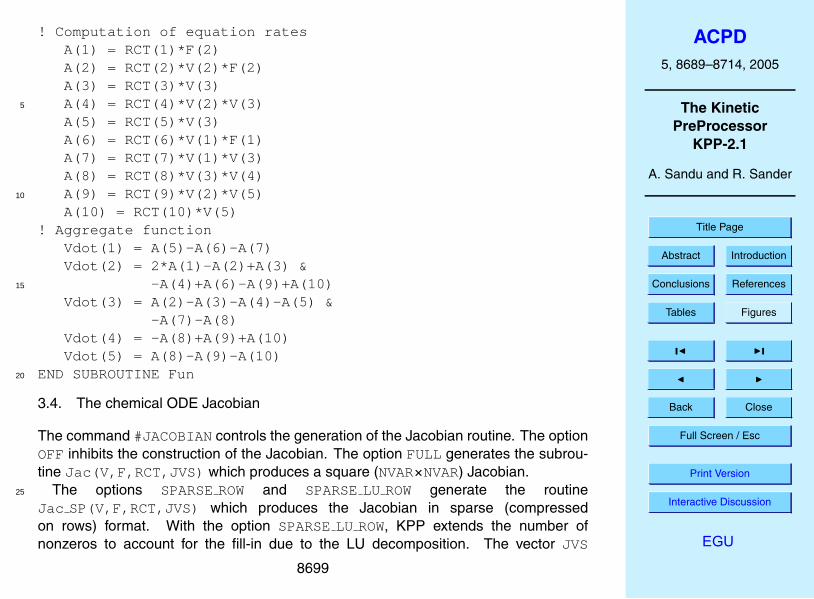
are parameters in the derivative function. KPP computes the vector A of reaction ratesand the vector Vdot of variable species time derivatives. The input arguments V andF are the concentrations of variable and fixed species, respectively. RCTcontains therate coefficients. Below is the Fortran90 code generated by KPP for the ODE functionof our example stratospheric system:20

SUBROUTINE Fun (V, F, RCT, Vdot )USE small_PrecisionUSE small_ParamsREAL(kind=DP) :: V(NVAR), &

F(NFIX), RCT(NREACT), &Vdot(NVAR), A(NREACT) &25

8698

ACPD5, 8689–8714, 2005

The KineticPreProcessor

KPP-2.1

A. Sandu and R. Sander

Title Page

Abstract Introduction

Conclusions References

Tables Figures

J I

J I

Back Close

Full Screen / Esc

Print Version

Interactive Discussion

EGU

! Computation of equation ratesA(1) = RCT(1)*F(2)A(2) = RCT(2)*V(2)*F(2)A(3) = RCT(3)*V(3)A(4) = RCT(4)*V(2)*V(3)5

A(5) = RCT(5)*V(3)A(6) = RCT(6)*V(1)*F(1)A(7) = RCT(7)*V(1)*V(3)A(8) = RCT(8)*V(3)*V(4)A(9) = RCT(9)*V(2)*V(5)10

A(10) = RCT(10)*V(5)! Aggregate function

Vdot(1) = A(5)-A(6)-A(7)Vdot(2) = 2*A(1)-A(2)+A(3) &

-A(4)+A(6)-A(9)+A(10)15

Vdot(3) = A(2)-A(3)-A(4)-A(5) &-A(7)-A(8)

Vdot(4) = -A(8)+A(9)+A(10)Vdot(5) = A(8)-A(9)-A(10)

END SUBROUTINE Fun20

3.4. The chemical ODE Jacobian

The command #JACOBIANcontrols the generation of the Jacobian routine. The optionOFF inhibits the construction of the Jacobian. The option FULL generates the subrou-tine Jac(V,F,RCT,JVS) which produces a square (NVAR×NVAR) Jacobian.

The options SPARSEROW and SPARSELU ROW generate the routine25

Jac SP(V,F,RCT,JVS) which produces the Jacobian in sparse (compressedon rows) format. With the option SPARSELU ROW, KPP extends the number ofnonzeros to account for the fill-in due to the LU decomposition. The vector JVS

8699

ACPD5, 8689–8714, 2005

The KineticPreProcessor

KPP-2.1

A. Sandu and R. Sander

Title Page

Abstract Introduction

Conclusions References

Tables Figures

J I

J I

Back Close

Full Screen / Esc

Print Version

Interactive Discussion

EGU

contains the LU NONZEROelements of the Jacobian in row order. Each row I starts atposition LU CROW(I) , and LU CROW(NVAR+1)=LUNONZERO+1. The location of theI -th diagonal element is LU DIAG(I) . The sparse element JVS(K) is the Jacobianentry in row LU IROW(K) and column LU ICOL(K) . The sparsity coordinate vectorsare computed by KPP and initialized statically. These vectors are constant as the5

sparsity pattern of the Hessian does not change during the computation.The routines Jac SP Vec(JVS,U,V) and JacTR SP Vec(JVS,U,V) perform

sparse multiplication of JVS (or its transpose) with a user-supplied vector U withoutany indirect addressing.

3.5. Sparse linear algebra10

To numerically solve for the chemical concentrations one must employ an implicittimestepping technique, as the system is usually stiff. Implicit integrators solve sys-tems of the form

Px = (I − hγJ)x = b (1)

where the matrix P=I−hγJ is refered to as the “prediction matrix”. I the identity matrix,15

h the integration time step, γ a scalar parameter depending on the method, and J thesystem Jacobian. The vector b is the system right hand side and the solution x typicallyrepresents an increment to update the solution.

The chemical Jacobians are typically sparse, i.e. only a relatively small number ofentries are nonzero. The sparsity structure of P is given by the sparsity structure of the20

Jacobian, and is produced by KPP with account for the fill-in. By carefully exploiting thesparsity structure, the cost of solving the linear system can be considerably reduced.

KPP orders the variable species such that the sparsity pattern of the Jacobian ismaintained after an LU decomposition. KPP defines a complete set of simulation pa-rameters, including the numbers of variable and fixed species, the number of chemical25

reactions, the number of nonzero entries in the sparse Jacobian and in the sparseHessian, etc.

8700

ACPD5, 8689–8714, 2005

The KineticPreProcessor

KPP-2.1

A. Sandu and R. Sander

Title Page

Abstract Introduction

Conclusions References

Tables Figures

J I

J I

Back Close

Full Screen / Esc

Print Version

Interactive Discussion

EGU

KPP generates the routine KppDecomp(P,IER) which performs an in-place, non-pivoting, sparse LU decomposition of the matrix P. Since the sparsity structure ac-counts for fill-in, all elements of the full LU decomposition are actually stored. Theoutput argument IER returns a nonzero value if singularity is detected.

The routines KppSolve(P,b,x) and KppSolveTR(P,b,x) use the LU factoriza-5

tion of P as computed by KppDecomp and perform sparse backward and forward sub-stitutions to solve the linear systems Px=b and PT

x=b, respectively. The KPP sparselinear algebra routines are extremely efficient, as shown in Sandu et al. (1996).

3.6. The chemical ODE Hessian

The Hessian contains second order derivatives of the time derivative functions. More10

exactly, the Hessian is a 3-tensor such that

HESSi ,j,k =∂2(Vdot)i∂Vj ∂Vk

, 1 ≤ i , j, k ≤ NVAR . (2)

With the command #HESSIAN ON, KPP produces the routineHessian(V,F,RCT,HESS) which calculates the Hessian HESS using the vari-able (V) and fixed (F) concentrations, and the rate coefficients (RCT).15

The Hessian is a very sparse tensor. KPP computes the number of nonzeroHessian entries (and saves this in the variable NHESS). The Hessian itself is rep-resented in coordinate sparse format. The real vector HESSholds the values, andthe integer vectors IHESS I , IHESS J , and IHESS K hold the indices of nonzero en-tries. Since the time derivative function is smooth, these Hessian matrices are sym-20

metric, HESS(I,J,K) =HESS(I,K,J) . KPP generates code only for those entriesHESS(I,J,K) with J≤K.

The sparsity coordinate vectors IHESS I , IHESS J , and IHESS K are computed byKPP and initialized statically. These vectors are constant as the sparsity pattern of theHessian does not change during the simulation.25

8701

ACPD5, 8689–8714, 2005

The KineticPreProcessor

KPP-2.1

A. Sandu and R. Sander

Title Page

Abstract Introduction

Conclusions References

Tables Figures

J I

J I

Back Close

Full Screen / Esc

Print Version

Interactive Discussion

EGU

The routines Hess Vec(HESS,U1,U2,HU) and HessTR Vec(HESS,U1,U2,HU)compute the action of the Hessian (or its transpose) on a pair of user-supplied vectorsU1, U2. Sparse operations are employed to produce the result vector HU.

3.7. The stoichiometric formulation

The command #STOICMAT ONinstructs KPP to generate a stoichiometric description5

of the chemical mechanism, which includes the stoichiometric matrix, the vector of re-actant products in each reaction, and partial derivatives with respect to concentrationsand to rate coefficients.

The stoichiometric matrix STOICMis constant and sparse. It is represented in sparse,column-compressed format. The routine ReactantProd computes the reactant prod-10

ucts for each reaction. The ODE function is given by the rate coefficients times thereactant products. The routine JacReactantProd computes the Jacobian of reactantproducts vector in row compressed sparse format.

3.8. The derivatives with respect to reaction coefficients

The stoichiometric formulation allows a direct computation of the derivatives with re-15

spect to rate coefficients. The routine dFun dRcoeff computes the partial derivativeof the ODE function with respect to a subset of the reaction coefficients. Similarlyone can obtain the partial derivative of the Jacobian with respect to a subset of therate coefficients. More exactly, with the subroutine dJac dRcoeff KPP generates theproduct of this partial derivative with a user-supplied vector.20

3.9. Utility routines

In addition to the chemical system description routines discussed above, KPP gener-ates several utility routines.

Probably the most often used subroutines are Initialize which sets the initial val-ues and Update RCONSTwhich updates the rate coefficients, e.g. according to current25

8702

ACPD5, 8689–8714, 2005

The KineticPreProcessor

KPP-2.1

A. Sandu and R. Sander

Title Page

Abstract Introduction

Conclusions References

Tables Figures

J I

J I

Back Close

Full Screen / Esc

Print Version

Interactive Discussion

EGU

temperature, pressure, and solar zenith angle.Reaction rates are calculated for all reactions of the chemical mechanism. This

information is available to the user and could be used, for example, to analyze thechemical mechanism and identify important reaction cycles as shown by Lehmann(2004).5

It was shown in Sect. 2.1 that each reaction in the #EQUATIONSsection may startwith an equation tag. With the command #EQNTAGS ON, KPP generates code thatconverts an equation tag to the internal reaction number assigned by KPP. It is alsopossible to obtain a string describing the chemical reaction. Thus the equation tagscan be used to refer to individual reactions.10

Shuffle kpp2user and Shuffle user2kpp convert a vector of concentrations inKPP ordering to one in user ordering and vice-versa.

3.10. KPP directory structure

The KPP distribution will unfold a directory with the following subdirectories:

– src/ contains the KPP source code.15

– bin/ contains the KPP executable. The path to this directory needs to be addedto the environment $PATH$variable.

– util/ contains different function templates useful for the simulation. Each tem-plate file has a suffix that matches the appropriate target language (.f90 , .f ,.c , or .m). KPP will run the template files through the substitution preprocessor.20

Users can define their own auxiliary functions by inserting them into the appropri-ate files.

– models/ contains the description of the chemical models. Users can define theirown models by placing the model description files in this directory. The KPPdistribution contains several models from atmospheric chemistry which can be25

used as examples for defining other models.

8703

ACPD5, 8689–8714, 2005

The KineticPreProcessor

KPP-2.1

A. Sandu and R. Sander

Title Page

Abstract Introduction

Conclusions References

Tables Figures

J I

J I

Back Close

Full Screen / Esc

Print Version

Interactive Discussion

EGU

– drv/ contains driver templates for chemical simulations. Each driver has a suffixthat matches the appropriate target language (.f90 , .f , .c , or .m). KPP will runthe driver through the substitution preprocessor. The driver template generalprovided with the distribution works with all examples. Users can define their owndriver templates here.5

– int/ contains numerical time stepping (integrator) routines. KPP searches thisdirectory for the definition file specified by the command #INTEGRATOR. Thisfile selects the numerical routine (with the #INTFILE command) and sets thefunction type, the Jacobian sparsity type, the target language, etc. Each integratortemplate is found in a file that ends with the appropriate suffix (.f90 , .f , .c , or10

.m). The selected template is processed by the substitution preprocessor. Userscan define here their own numerical integration routines.

– examples/ contains several model description examples which can be used astemplates for building simulations with KPP.

– site-lisp/ contains the file kpp.el which provides a KPP mode for emacs15

with color highlighting.

4. Language-specific code generation

The code generated by KPP for the kinetic model description is organized in a set ofseparate files. The files associated with the model ROOT are named with the prefix“ROOT ”. A list of KPP-generated files is shown in Table 1.20

4.1. Fortran90

The generated code is consistent with the Fortran90 standard. It will not exceed themaximum number of 39 continuation lines. If KPP cannot properly split an expression

8704

ACPD5, 8689–8714, 2005

The KineticPreProcessor

KPP-2.1

A. Sandu and R. Sander

Title Page

Abstract Introduction

Conclusions References

Tables Figures

J I

J I

Back Close

Full Screen / Esc

Print Version

Interactive Discussion

EGU

to keep the number of continuation lines below the threshold then it will generate awarning message pointing to the location of this expression.

The driver file ROOT Main.f90 contains the main Fortran90 program. All other codeis enclosed in Fortran modules. There is exactly one module in each file, and the nameof the module is identical to the file name but without the suffix .f90 .5

Fortran90 code uses parameterized real types. KPP generates the moduleROOT Precision which contains the single and double real kind definitions:

INTEGER, PARAMETER :: &SP = SELECTED_REAL_KIND(6,30), &DP = SELECTED_REAL_KIND(12,300)10

Depending on the user choice of the #DOUBLEswitch the real variables are of typedouble or single precision. Changing the parameters of the SELECTEDREAL KINDfunction in this module will cause a change in the working precision for the wholemodel.

The global parameters (Sect. 3.1) are defined and initialized in the module15

ROOT Parameters . The global variables (Sect. 3.2) are declared in the moduleROOT Global . They can be accessed from within each program unit that uses theglobal module.

The sparse data structures for the Jacobian (Sect. 3.4) are declared and initialized inthe module ROOT JacobianSP . The sparse data structures for the Hessian (Sect. 3.6)20

are declared and initialized in the module ROOT HessianSP .The code for the ODE function (Sect. 3.3) is in module ROOT Function . The

code for the ODE Jacobian and sparse multiplications (Sect. 3.4) is in mod-ule ROOT Jacobian . The Hessian function and associated sparse multiplications(Sect. 3.6) are in module ROOT Hessian .25

The module ROOT Stoichiom contains the functions for reactant products and itsJacobian (Sect. 3.7), and derivatives with respect to rate coefficients (Sect. 3.8). Thedeclaration and initialization of the stoichiometric matrix and the associated sparsedata structures (Sect. 3.7) is done in the module ROOT StoichiomSP .

8705

ACPD5, 8689–8714, 2005

The KineticPreProcessor

KPP-2.1

A. Sandu and R. Sander

Title Page

Abstract Introduction

Conclusions References

Tables Figures

J I

J I

Back Close

Full Screen / Esc

Print Version

Interactive Discussion

EGU

Sparse linear algebra routines (Sect. 3.5) are in the module ROOT LinearAlgebra .The code to update the rate constants and the user defined rate law functions arein module ROOT Rates . The utility and input/output functions (Sect. 3.9) are inROOT Util and ROOT Monitor .

Matlab-mex gateway routines for the ODE function, Jacobian, and Hessian are dis-5

cussed in Sect. 4.5.

4.2. Matlab

Matlab code allows for rapid prototyping of chemical kinetic schemes, and for a con-venient analysis and visualization of the results. Differences between different kineticmechanisms can be easily understood. The Matlab code can be used to derive refer-10

ence numerical solutions, which are then compared against the results obtained withuser-supplied numerical techniques. Last but not least Matlab is an excellent environ-ment for educational purposes. KPP/Matlab can be used to teach students fundamen-tals of chemical kinetics and chemical numerical simulations.

Each Matlab function has to reside in a separate m-file. Function calls use the m-15

function-file names to reference the function. Consequently, KPP generates one m-function-file for each of the functions discussed in Sects. 3.3, 3.4, 3.5, 3.6, 3.7, 3.8,and 3.9. The names of the m-function-files are the same as the names of the functions(prefixed by the model name ROOT).

The global parameters (Sect. 3.1) are defined as Matlab global variables and ini-20

tialized in the file ROOT parameter defs.m . The global variables (Sect. 3.2) aredeclared as Matlab global variables in the file ROOT Global defs.m . They canbe accessed from within each Matlab function by using global declarations of thevariables of interest.

The sparse data structures for the Jacobian (Sect. 3.4), the Hessian (Sect. 3.6),25

the stoichiometric matrix and the Jacobian of reaction products (Sect. 3.7) are de-clared as Matlab global variables in the file ROOT Sparse defs.m . They are ini-tialized in separate m-files, namely ROOT JacobianSP.m ROOT HessianSP.m , and

8706

ACPD5, 8689–8714, 2005

The KineticPreProcessor

KPP-2.1

A. Sandu and R. Sander

Title Page

Abstract Introduction

Conclusions References

Tables Figures

J I

J I

Back Close

Full Screen / Esc

Print Version

Interactive Discussion

EGU

ROOT StoichiomSP.m respectively.Two wrappers (ROOT Fun Chem.mand ROOT Jac SP Chem.m) are provided for in-

terfacing the ODE function and the sparse ODE Jacobian with Matlab’s suite of ODEintegrators. Specifically, the syntax of the wrapper calls matches the syntax required byMatlab’s integrators like ode15s. Moreover, the Jacobian wrapper converts the sparse5

KPP format into a Matlab sparse matrix.

4.3. C

The driver file ROOT Main.c contains the main driver and numerical integrator func-tions, as well as declarations and initializations of global variables (Sect. 3.2).

The generated C code includes three header files which are #include -d in10

other files as appropriate. The global parameters (Sect. 3.1) are #define -d inthe header file ROOT Parameters.h . The global variables (Sect. 3.2) are extern-declared in ROOT Global.h , and declared in the driver file ROOT.c . The header fileROOT Sparse.h contains extern declarations of sparse data structures for the Jaco-bian (Sect. 3.4), Hessian (Sect. 3.6), stoichiometric matrix and the Jacobian of reaction15

products (Sect. 3.7). The actual declarations of each data structures is done in the cor-responding files.

The code for each of the model functions, integration routine, etc. is located in thecorresponding file (with extension .c ) as shown in the Table 1.

Finally, Matlab mex gateway routines that allow the C implementation of the ODE20

function, Jacobian, and Hessian to be called directly from Matlab (Sect. 4.5) are alsogenerated.

4.4. Fortran77

The general layout of the Fortran77 code is similar to the layout of the C code. Thedriver file ROOT Main.f contains the main program and the initialization of global vari-25

ables.

8707

ACPD5, 8689–8714, 2005

The KineticPreProcessor

KPP-2.1

A. Sandu and R. Sander

Title Page

Abstract Introduction

Conclusions References

Tables Figures

J I

J I

Back Close

Full Screen / Esc

Print Version

Interactive Discussion

EGU

The generated Fortran77 code includes three header files. The global pa-rameters (Sect. 3.1) are defined as parameters and initialized in the headerfile ROOT Parameters.h . The global variables (Sect. 3.2) are declared inROOT Global.h as common block variables. There are global common blocks forreal (GDATA), integer (INTGDATA), and character (CHARGDATA) global data. They can5

be accessed from within each program unit that includes the global header file.The header file ROOT Sparse.h contains common block declarations of sparse data

structures for the Jacobian (Sect. 3.4), Hessian (Sect. 3.6), stoichiometric matrix andthe Jacobian of reaction products (Sect. 3.7). These sparse data structures are initial-ized in four named “block data” statements.10

The code for each of the model functions, integration routine, etc. is located in thecorresponding file (with extension .f ) as shown in the Table 1.

Matlab-mex gateway routines for the ODE function, Jacobian, and Hessian are dis-cussed in Sect. 4.5.

4.5. Mex interfaces15

KPP generates mex gateway routines for the ODE function (ROOT mex Fun), Jacobian(ROOT mex Jac SP), and Hessian (ROOT mex Hessian ), for the target languages C,Fortran77, and Fortran90.

After compilation (using Matlab’s mex compiler) the mex functions can be calledinstead of the corresponding Matlab m-functions. Since the calling syntaxes are identi-20

cal, the user only has to insert the “mex” string within the corresponding function name.Replacing m-functions by mex-functions gives the same numerical results, but the com-putational time could be considerably shorter, especially for large kinetic mechanisms.

If possible we recommend to build mex files using the C language, as Matlab offersmost mex interface options for the C language. Moreover, Matlab distributions come25

with a native C compiler (lcc) for building executable functions from mex files. For-tran77 mex files work well on most platforms without additional efforts. The mex filesbuilt using Fortran90 may require further platform-specific tuning of the mex compiler

8708

ACPD5, 8689–8714, 2005

The KineticPreProcessor

KPP-2.1

A. Sandu and R. Sander

Title Page

Abstract Introduction

Conclusions References

Tables Figures

J I

J I

Back Close

Full Screen / Esc

Print Version

Interactive Discussion

EGU

options.

5. Applications

In this section we illustrate several applications using KPP.

5.1. Benchmark tests

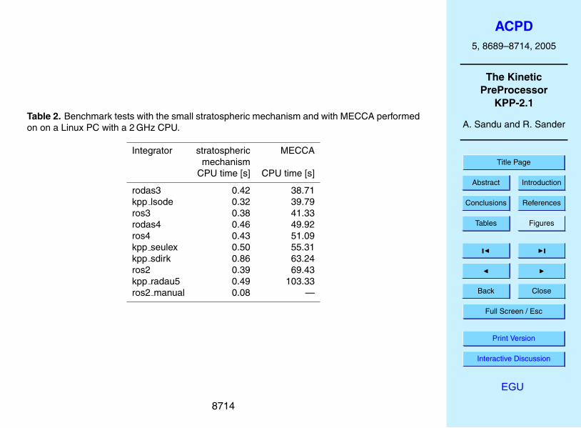
We performed some model runs to test the stability and efficiency of the KPP inte-5

grators. First, we used the very simple Chapman-like stratospheric mechanism. Sim-ulations of one month were made using the 10 different integrators ros2, ros3, ros4,rodas3, rodas4, ros2 manual, kpp radau5, kpp sdirk, kpp seulex, and kpp lsode. TheCPU times used for the runs are shown in Table 2. Radau5, the most accurate inte-grator, is also the slowest. Since the overhead for the automatic time step control is10

relatively large in this small mechanism, the integrator ros2 manual with manual timestep control is by far the fastest here. However, it is also the least precise integrator,when compared to Radau5 as reference.

As a second example, we have performed runs with the complex chemistry modelMECCA (Sander et al., 2005) simulating gas and aerosol chemistry in the marine15

boundary layer. We have selected a subset of the MECCA mechanism with 212species, 106 gas-phase reactions, 266 aqueous-phase reactions, 154 heterogeneousreactions, 37 photolyses, and 48 aqueous-phase equilibria. The CPU times for 8-daysimulations with different integrators are shown in Table 2. Again, Radau5 is the slow-est integrator. The Rosenbrock integrators with automatic time step control and LSODE20

are much faster. The integrator ros2 manual with manual time step control was unableto solve this very stiff system of differential equations.

8709

ACPD5, 8689–8714, 2005

The KineticPreProcessor

KPP-2.1

A. Sandu and R. Sander

Title Page

Abstract Introduction

Conclusions References

Tables Figures

J I

J I

Back Close

Full Screen / Esc

Print Version

Interactive Discussion

EGU

5.2. Direct and adjoined sensitivity studies

KPP has recently been extended with the capability to generate code for direct andadjoint sensitivity analysis. This was described in detail by Sandu et al. (2003) andDaescu et al. (2003). Here, we only briefly summarize these features. The direct de-coupled method, build using backward difference formulas (BDF), has been the method5

of choice for direct sensitivity studies. The direct decoupled approach was extendedto Rosenbrock stiff integration methods. The need for Jacobian derivatives preventedRosenbrock methods to be used extensively in direct sensitivity calculations. However,the new automatic differentiation and symbolic differentiation technologies make thecomputation of these derivatives feasible. The adjoint modeling is an efficient tool to10

evaluate the sensitivity of a scalar response function with respect to the initial con-ditions and model parameters. In addition, sensitivity with respect to time dependentmodel parameters may be obtained through a single backward integration of the adjointmodel. KPP software may be used to completely generate the continuous and discreteadjoint models taking full advantage of the sparsity of the chemical mechanism. Flex-15

ible direct-decoupled and adjoint sensitivity code implementations are achieved withminimal user intervention.

6. Conclusions

The widely-used software environment KPP for the simulation of chemical kinetics wasadded the capabilities to generate simulation code in Fortran90 and Matlab. An up-20

date of the Fortran77 and C generated code was also performed. The new capabilitieswill allow researchers to include KPP generated modules in state-of-the-art large scalemodels, for example in the field of air quality studies. Many of these models are im-plemented in Fortran90. The Matlab capabilities will allow for a rapid prototyping ofchemical kinetic systems, and for the visualization of the results. Matlab also offers an25

ideal educational environment and KPP can be used in this context to teach introduc-

8710

ACPD5, 8689–8714, 2005

The KineticPreProcessor

KPP-2.1

A. Sandu and R. Sander

Title Page

Abstract Introduction

Conclusions References

Tables Figures

J I

J I

Back Close

Full Screen / Esc

Print Version

Interactive Discussion

EGU

tory chemistry or modeling classes.The KPP-2.1 source code is distributed under the provisions of the GNU public li-

cense (http://www.gnu.org/copyleft/gpl.html) and is available in the electronic supple-ment to this paper at http://www.atmos-chem-phys.org/acpd/5/8689/acpd-5-8689-sp.zip. The source code and the documentation can also be obtained from http://people.5

cs.vt.edu/∼asandu/Software/Kpp.

Acknowledgements. The work of A. Sandu was supported by the awards NSF-CAREER ACI0413872 and NSF-ITR AP&IM 0205198.

References

Brown, P., Byrne, G., and Hindmarsh, A.: VODE: A Variable Step ODE Solver, SIAM J. Sci.10

Stat. Comput., 10, 1038–1051, 1989. 8696Curtis, A. R. and Sweetenham, W. P.: Facsimile/Chekmat User’s Manual, Tech. rep., Computer

Science and Systems Division, Harwell Lab., Oxfordshire, Great Britain, 1987. 8690Daescu, D., Sandu, A., and Carmichael, G. R.: Direct and adjoint sensitivity analysis of chem-

ical kinetic systems with KPP: II – Validation and numerical experiments, Atmos. Environ.,15

37, 5097–5114, 2003. 8710Damian, V., Sandu, A., Damian, M., Carmichael, G. R., and Potra, F. A.: KPP – A symbolic

preprocessor for chemistry kinetics – User’s guide, Technical report, The University of Iowa,Iowa City, IA 52246, 1995. 8690

Damian, V., Sandu, A., Damian, M., Potra, F., and Carmichael, G. R.: The kinetic preprocessor20

KPP – a software environment for solving chemical kinetics, Comput. Chem. Eng., 26, 1567–1579, 2002. 8690

Djouad, R., Sportisse, B., and Audiffren, N.: Reduction of multiphase atmospheric chemistry,J. Atmos. Chem., 46, 131–157, 2003. 8690

Hairer, E. and Wanner, G.: Solving Ordinary Differential Equations II. Stiff and Differential-25

Algebraic Problems, Springer-Verlag, Berlin, 1991. 8695Lehmann, R.: An algorithm for the determination of all significant pathways in chemical reaction

systems, J. Atmos. Chem., 47, 45–78, 2004. 8703

8711

ACPD5, 8689–8714, 2005

The KineticPreProcessor

KPP-2.1

A. Sandu and R. Sander

Title Page

Abstract Introduction

Conclusions References

Tables Figures

J I

J I

Back Close

Full Screen / Esc

Print Version

Interactive Discussion

EGU

Leis, J. and Kramer, M.: ODESSA – An Ordinary Differential Equation Solver with ExplicitSimultaneous Sensitivity Analysis, ACM Transactions on Mathematical Software, 14, 61–67,1986. 8696

Radhakrishnan, K. and Hindmarsh, A.: Description and use of LSODE, the Livermore solverfor differential equations, NASA reference publication 1327, 1993. 8695, 86965

Sander, R., Kerkweg, A., Jockel, P., and Lelieveld, J.: Technical Note: The new comprehensiveatmospheric chemistry module MECCA, Atmos. Chem. Phys., 5, 445–450, 2005,SRef-ID: 1680-7324/acp/2005-5-445. 8690, 8709

Sandu, A., Potra, F. A., Damian, V., and Carmichael, G. R.: Efficient implementation of fullyimplicit methods for atmospheric chemistry, J. Comp. Phys., 129, 101–110, 1996. 870110

Sandu, A., Verwer, J. G., Blom, J. G., Spee, E. J., Carmichael, G. R., and Potra, F. A.: Bench-marking stiff ODE solvers for atmospheric chemistry problems II: Rosenbrock solvers, Atmos.Environ., 31, 3459–3472, 1997. 8695

Sandu, A., Daescu, D., and Carmichael, G. R.: Direct and adjoint sensitivity analysis of chemi-cal kinetic systems with KPP: I – Theory and software tools, Atmos. Environ., 37, 5083–5096,15

2003. 8692, 8710Tang, Y., Carmichael, G. R., Uno, I., Woo, J.-H., Kurata, G., Lefer, B., Shetter, R. E., Huang,

H., Anderson, B. E., Avery, M. A., Clarke, A. D., and Blake, D. R.: Impacts of aerosolsand clouds on photolysis frequencies and photochemistry during TRACE-P: 2. Three-dimensional study using a regional chemical transport model, J. Geophys. Res., 108(D21),20

doi:10.1029/2002JD003100, 2003. 8690Trentmann, J., Andreae, M. O., and Graf, H.-F.: Chemical processes in a young biomass-

burning plume, J. Geophys. Res., 108(D22), doi:10.1029/2003JD003732, 2003. 8690Verwer, J., Spee, E., Blom, J. G., and Hunsdorfer, W.: A second order Rosenbrock method

applied to photochemical dispersion problems, SIAM Journal on Scientific Computing, 20,25

1456–1480, 1999. 8695von Glasow, R., Sander, R., Bott, A., and Crutzen, P. J.: Modeling halogen chemistry

in the marine boundary layer. 1. Cloud-free MBL, J. Geophys. Res., 107(D17), 4341,doi:10.1029/2001JD000942, 2002. 8690

von Kuhlmann, R., Lawrence, M. G., Crutzen, P. J., and Rasch, P. J.: A model for studies of30

tropospheric ozone and nonmethane hydrocarbons: Model description and ozone results, J.Geophys. Res., 108(D9), doi:10.1029/2002JD002893, 2003. 8690

8712

ACPD5, 8689–8714, 2005

The KineticPreProcessor

KPP-2.1

A. Sandu and R. Sander

Title Page

Abstract Introduction

Conclusions References

Tables Figures

J I

J I

Back Close

Full Screen / Esc

Print Version

Interactive Discussion

EGU

Table 1. List of KPP-generated files (for Fortran90).

File Description

ROOT Main.f90 Driver

ROOT Precision.f90 Parameterized typesROOT Parameters.f90 Model parametersROOT Global.f90 Global data headersROOT Monitor.f90 Equation infoROOT Initialize.f90 InitializationROOT Model.f90 Summary of modules

ROOT Function.f90 ODE function

ROOT Jacobian.f90 ODE JacobianROOT JacobianSP.f90 Jacobian sparsity

ROOT Hessian.f90 ODE HessianROOT HessianSP.f90 Sparse Hessian data

ROOT LinearAlgebra.f90 Sparse linear algebraROOT Integrator.f90 Numerical integration

ROOT Stoichiom.f90 Stoichiometric modelROOT StoichiomSP.f90 Stoichiometric matrix

ROOT Rates.f90 User-defined rate lawsROOT Util.f90 Utility input-outputROOT Stochastic.f90 Stochastic functions

Makefile ROOT Makefile

ROOT.map Human-readable info

8713

ACPD5, 8689–8714, 2005

The KineticPreProcessor

KPP-2.1

A. Sandu and R. Sander

Title Page

Abstract Introduction

Conclusions References

Tables Figures

J I

J I

Back Close

Full Screen / Esc

Print Version

Interactive Discussion

EGU

Table 2. Benchmark tests with the small stratospheric mechanism and with MECCA performedon on a Linux PC with a 2 GHz CPU.

Integrator stratospheric MECCAmechanism

CPU time [s] CPU time [s]

rodas3 0.42 38.71kpp lsode 0.32 39.79ros3 0.38 41.33rodas4 0.46 49.92ros4 0.43 51.09kpp seulex 0.50 55.31kpp sdirk 0.86 63.24ros2 0.39 69.43kpp radau5 0.49 103.33ros2 manual 0.08 —

8714