Embed Size (px)
Citation preview
Technical Efficiency of Fruit and Vegetable Producers in Tamil Nadu, India: A Stochastic Frontier ApproachSrinivasulu RajendranAVRDC - The World Vegetable Center, Eastern and Southern AfricaEmail: [email protected]
ABSTRACT
In India, fruits and vegetables (F&V) significantly contribute to food and nutritional security; they also enhance the livelihoods of smallholders. In recent years, demand has been increasing for these important crops, yet their productivity has been decelerating. Technical innovations can reduce yield gaps and increase the productivity of F&V crops. This paper measures technical efficiency (TE) of F&V production and its determinants based on Cobb-Douglas stochastic frontier production function. TE is defined as the maximum output that can be produced from a specified set of inputs, given the existing technology available to the farmer. The study surveyed a sample of 240 households who mostly cultivate F&V in Salem, Trichy, and Theni districts, Tamil Nadu. Mean TE level was estimated to be 0.60. The farmers in Trichy had higher TEs than those in the other districts. This means Trichy farmers use inputs more efficiently. If the average farmer in the sample could achieve the TE level of his/her most efficient counterpart, then he/she could increase output by about 34 percent with the same level of inputs. There is considerable room for increasing F&V output without additional inputs. Accessibility of irrigation facilities significantly contributed to the higher TE in Trichy. While the test for equality showed that TE did not vary significantly across farm sizes, the larger landholdings had higher TE than smaller landholdings, indicating that farm size and TE are directly related. The results showed that accessibility of infrastructure facilities (e.g., road) contributed positively to TE. Other variables such as level of education and access to credit also had positive relationship with TE.
Keywords: technical efficiency, production efficiency, stochastic frontier JEL Classification: Q12, Q18

78 Srinivasulu Rajendran
INTRODUCTION
India is the largest producer of fruits and vegetables (F&V) in the world, accounting for 12.5 and 9.7 percent, respectively, of the world’s production in 2010 (FAO 2012). The share of F&V to the real value (at 2004–2005 prices) of agricultural output increased from 19.2 to 26.3 percent between 1981 and 2009. Annual growth rate of the F&V value increased from 2.3 to 4.3 percent between 1981–1990 and 1991–2009 (CSO 2012). In 2009–2010, F&V became the single largest subsector in horticultural crops, accounting for 68.6 percent of the area under horticulture (MoA 2011). On the demand side, National Sample Survey data show that the share of monthly per capita expenditure on F&V increased from 12.2 percent in 1993–1994 to 14.6 percent in 2009–2010 in rural areas, and from 14.9 percent to 15.7 percent in urban areas (CSO 2012). The Agricultural Census (2000–2001) reports that small farmers (<2 ha) had allocated 5.7 percent of their total cropped area to horticultural crops, compared with 3.9 percent of the large farmers (>4 ha). Further, over the same period, the share of horticultural crops in the small farmers’ total cropped area had increased, though proportionately less than that of medium and large farmers.
Many studies show that Indian farmers prefer F&V production to other crops because of better returns. F&V production has been found to also contribute more to the well-being of farmers, particularly smallholders, due to its labor intensive nature, which generates more employment (Birthal et al. 2012; Birthal et al. 2008; Mittal 2007; Joshi, Tewari, and Birthal 2006; Singh et al. 2004; Kumar 1998; Kumar and Mathur 1996). On the other hand, though the share of F&V in gross cropped area increased from 2.8 to 4.9 percent between 1981 and 2006 and the share in output from 16.0 to 25.8 percent, productivity growth decelerated
(Chand, Raju, and Pandey 2008). To address this slowdown, the Government of India began a major initiative in 2004 under the National Horticulture Mission to increase the share of horticulture in total food and nonfood crops, improve yields, and ensure better returns to farmers.
This paper aims to measure technical efficiency (TE) of farming households that mainly grow F&V crops in Tamil Nadu state and to identify determinants of technical inefficiency. To achieve these objectives, the following hypotheses were constructed and examined: (1) output increases proportionately with increase in inputs; (2) a significant inverse relationship exists between farm size and TE; and (3) technical inefficiency is negatively and significantly determined by education, access to extension, inputs, credit services, and infrastructural facilities. The paper is divided into four sections. The first section provides a background on the study and section 2 focuses on data requirements and the methodological aspects. Section 3 explains the empirical results of TE based on household data on outputs and inputs used in crop cultivation. Section 4 sums up the findings and draws broad conclusions.
METHODOLOGY
Data Source and Survey Methodology
A farm household survey was conducted from December 2010 to February 2011 to gather data on crop year July 2009–June 2010. Respondents were 240 households cultivating F&V in Salem, Trichy, and Theni districts in Tamil Nadu, India. Systematic random sampling technique was used to select the sample households. It was purposively decided to survey 100 households in each district (Appendix Table 1 and Appendix Table 2). After eliminating data outliers and considering 100
Asian Journal of Agriculture and Development, Vol. 11, No. 1 79
percent participation of farmers in the survey, only 80 households from each district (total of 240 households) were used in the analysis. The survey was done in three stages: pre-pilot, pilot, and main survey using a questionnaire drawn up after interaction with officials concerned from several departments and academic institutions. A pre-pilot survey was done in Salem in August 2010. The questionnaire was improved based on the outcome of the pre-pilot survey. A pilot survey to test the questionnaire was then conducted in Salem in November 2010. The questionnaire was further modified based on the problems experienced and results of the pilot survey. The main survey was conducted in Salem, Trichy, and Theni between November 2010 and February 2011. Meetings with officials in horticulture and agriculture departments in the respective study areas were conducted to identify the blocks and villages to be surveyed.
Econometric Framework
The first objective of this paper is to measure TE by adopting a stochastic frontier production (SFP) function, which was originated from the theoretical work of Debreu (1951) and Farrell (1957); Aigner, Lovell, and Schmidt (1977) and Meeusen and van den Broeck (1977) extended the deterministic frontier approach to account for technical inefficiency, as well as for any measurement errors or statistical noise. This approach offers some advantages over other
methods generally used in efficiency analysis. For one, it is easy to implement and interpret. More importantly, it allows segregating the effect of statistical noises from systematic sources of inefficiency. Besides, the technique is consistent with most of the agricultural production efficiency studies.
The parameters of the SFP functions model are estimated by the method of maximum likelihood (ML) shown in equation (1)1.
Battese and Tessema (1993) argue that if any input costs were 0, those particular costs are included in the total input cost in the functions. Therefore, cost of machinery, which had a high proportion of zero observations in all three districts (accordingly, the sample means were not large enough), was added in the total input costs category.
Specified as the value of output, value of crop production is defined as total output value (in Indian rupees [INR]) realized from total crop production.2 Gross value of output, defined as gross value of aggregate output of all the individual crops and their by-products, is the dependent variable. Both outputs and inputs were measured in value (INR) terms only. Actual prices received by the farmers were used to value aggregate production.
1 where i =1,…,N (number of households), k =1,…,N (number of inputs) and where the dependent variable output (value of crop production) Yi and independent variables, which include inputs Xk, are defined as follows: Ln is the natural logarithm with base e, value of crop production Y per household (in rupees): Y = value of crop production, inputs X per household (cost in rupees): X1 = land: net operated area in acres, X2 = cost of seed, X3 = cost of manure, X4 = cost of fertilizer, X5 = cost of chemicals, X6 = cost of labor, X7 = cost of machinery (i.e., tractor and other equipment), X6 = share of area under irrigation, Di = dummy variable for districts, vi are the random variables associated with disturbances in production; ui are non-negative random variables associated with the technical inefficiency of the ith farmer. 2 This choice was made considering the argument of Abdulai and Tietje (2007) that using output value rather than output by itself has the advantage of taking quality differences into account. It also notes the argument of Sharma (1992) that taking account of production of all crops is more useful than single-crop production in the production function because the single-crop production functions do not account for indirect production benefits.
80 Srinivasulu Rajendran
Noting that land is the most important and a limiting factor in Indian agriculture, this study considered the households’ net operated area (NOA) in the frontier model.
Coelli and Battese (1996) argue that the cost of inputs includes the cost of fertilizer, pesticide, manure, and machinery and that it is desirable to have data on these individual inputs because each holds a significant influence on crop production. As such, this study considered the cost of inputs individually to capture the individual effects on mean value of output per household, particularly farmer’s expenditure on seeds, fertilizers, pesticide, manure, machinery, and labor. The share of area under irrigation was included for the analysis as a physical variable.
The total cost of labor for crop production per farm household is used.
All variables are in value terms, except for NOA and share of area under irrigation. Following Kumar and Sarkar (2012), the study calculated the value of each variable using actual prices paid by farmers at the time of farm operations. After deciding on the mode of selection of inputs, one important step remained to be considered: to test the hypotheses of the stochastic frontier production (SFP) approach suggested by Coelli and Battese (1996), who posit that the inefficiency model can only be estimated if inefficiency effects are stochastic and have a particular distributional specification.
Model Specifications for Determinants of Inefficiency
Isolating the sources of inefficiency could play an important role in designing policies to improve efficiency. Literature indicates a range of socioeconomic and infrastructure factors determining inefficiency, including land use, credit, land tenure, and household education (Seyoum, Battese, and Fleming 1998; Battese and Coelli 1995; Coelli and Battese 1996; Kumbhakar 1994); and techniques of cultivation, share tenancy, and landholding size
(Ali and Choudhury 1990; Coelli and Battese 1996; Kumbhakar 1994). Some environmental and nonphysical factors like information availability, experience, and farm supervision may also affect producers’ capability to efficiently use available technology (Parikh, Ali, and Shah 1995; Kumbhakar 1994). This study identifies factors associated with technical inefficiency based on a single-stage or single-step approach equation suggested by Battese and Coelli (1995). Iraizoz, Rapun, and Zabaleta (2003) indicate two basic approaches to accounting for the effects of exogenous variables. One is a one-step or single-stage procedure that directly includes the exogenous variables (Battese and Coelli 1995). The other is a two-step or two-stage approach, which first estimates the relative efficiencies using inputs and outputs and then analyzes the effects of the exogenous variables on inefficiency (McCarty and Yaisawarng 1993).
This paper uses the single-stage procedure, which as Battese and Coelli (1995) argue, has more advantage than the two-stage approach in that it includes frontier and technical inefficiency models together and estimates simultaneously.
(2)
where i =1,…, N (number of households), k = 1,…, N (number of inputs), D = regional dummies.
Land represents the total area of irrigated and unirrigated land (in acres); IL represents total area of irrigated land that is operated (in acres); from equation (3) it is assumed that the inefficiency effects are independently distributed and Ui arises by truncation (at zero) of the normal distribution with mean µi and variance σ2, where µi is defined as:
(3)
Asian Journal of Agriculture and Development, Vol. 11, No. 1 81
where: zmi = socioeconomic characteristics of the farm households;3 m = 1,..., j (number of households); i =,…, n (explanatory variables).
Family size
Is family size significantly correlated with technical inefficiency, as pointed out by Bravo-Ureta and Pinheiro (1997)? This paper adopted the proposition of Villano and Fleming (2004) that it is useful to have a ratio of adult members of the household because this coefficient is expected to have a negative effect on technical inefficiency; that is, having more adult members means more quality labor available, thus making the production process more efficient.
Age of farmer
Coelli (1996) concluded that age is expected to have both positive and negative effects on efficiency. Older farmers are likely to have had more farming experience but could be less receptive to adopting new technologies and practices (Coelli and Battese 1996; Abdulai and Huffman 2000). Bravo-Ureta and Pinheiro (1997) argue that younger farmers are likely to have some formal education and, therefore, might have more success in gathering information and understanding new practices, which, in turn, will improve their economic efficiency through higher TE.
Net effect of non-farm work on inefficiency
Abdulai and Huffman (2000) argue that the net effect of non-farm work on inefficiency is ambiguous, since it may restrict production and decision-making activities, thereby increasing inefficiency. But they also maintain that increased non-farm work reduces
financial constraints, particularly for resource-poor farmers, and enables them to purchase productivity-enhancing inputs. This study has included farm activities dummy in the model to capture the net effect of participation in non-farm labor markets on inefficiency.
Education level of head of household
Do farmers exposed to new technologies and improved techniques with education and extension services perform better (Coelli and Battese 1996; Asogwa, Ihemeje, and Ezihe 2011; Abdulai and Huffman 2000)? Lockheed, Jamison, and Lau (1980) hypothesized education to have a negative impact on inefficiency. Huffman (1974) said that this “allocative ability,” which stems from reallocation of resources in response to changes in economic conditions, requires: (1) perceiving that change has occurred; (2) collecting, retrieving, and analyzing useful information; (3) drawing valid conclusions from available information; and (4) acting quickly and decisively. Educational level and extension services are directly related to Indian farmers’ allocative efficiency (Ram 1980).
Access to formal credit
Access to formal credit enables a farmer to overcome financial constraints (Abdulai and Huffman 2000) and increases the net revenue obtained from fixed inputs, market conditions, and individual characteristics. Credit constraints limit the adoption of high-yielding varieties and acquisition of information needed for increased productivity; however, credit has no effect on production if it simply displaces another source of financing such as savings.
3 Z1 = age of household head; Z2 = ratio of adult members of household family size; Z3 = household head’s literacy level (1 = literate, 0 = otherwise); Z4 = extension contact (1 = farmer has had permanent contact with an agricultural extension officer in the past year, 0 = otherwise); Z5 = access to credit (1 = farmer has had cash credit in the past year, 0 = otherwise); Z6 = level of occupation (1 = non-farm, 0 = otherwise); Z7 = net operated area; Z8 = distance from farm to main road (km); Z9 = gender (1 = male, 0 = female); Dd = district dummies (D1 = Salem [slope dummy], D2 = Trichy, D3 = Theni).
82 Srinivasulu Rajendran
Credit can negatively impact profits if lenders treat it as a welfare program because farmers tend to perceive default costs as minor. Given the above, this study considers credit as an explanatory variable in its model.
Land
This study has adopted NOA as indicator for impact of land on value of output. The larger the farm size, the greater is the opportunity to apply new technologies such as tractors and irrigation. While the sign of the coefficient of land is expected to be negative, it may turn out positive as small farmers could have alternative income sources (Coelli and Battese 1996). Bhalla (1987), Bhalla and Chadha (1983), Shergill (1987), and Sharma (1992), on the other hand, argue that other than use of machinery, large farm landholders put in more material inputs than small farm landholders, resulting in increased productivity. The implication is that medium and large farms derive more gains from application of more capital than do small farms. This may be because, on account of land and other constraints, small farm landholders cannot make use of improved or better inputs. On the other hand, the above studies also argue that small farm landholders are more efficient in land management. This may be because of more intensive cultivation with family labor or because their land is more fertile than larger farm lands.
Access to infrastructure and gender, etc.
Access to infrastructure and gender, among others, are useful in examining the determinants of inefficiency (Coelli and Battese 1996; Abdulai and Huffman 2000). The household head, whether male or female, is the primary decision-maker.
Abdulai and Huffman (2000) contend that factors contributing to relatively higher efficiency include: (1) easier access to information because of favorable location of
extension services, improved seed multiplication units, agricultural financial institutions, and fertilizer depots in the more accessible districts; (2) better health and water facilities; and (3) greater market access. Farmers located in districts characterized by such facilities are exposed to modernizing environments where new crop varieties, innovative planting methods, and capital inputs (e.g., insecticides, tractors or machines) are readily available. In agreement, the study included district-level dummies in the model to capture the impact of locational characteristics on inefficiency.
Schultz (1964) posits that if a farm is located relatively far from the regional market, the farmer uses more time to obtain inputs and the purchase price (gross of transport costs) is higher, all of which affects technical inefficiency. Farmers with very poor access to markets for consumer goods also tend to be less interested in profit-maximizing activities compared with those living in areas with a sufficient supply of consumer goods. In agreement with this argument, this study included distance from farm to main road in the model.
RESULTS AND DISCUSSION
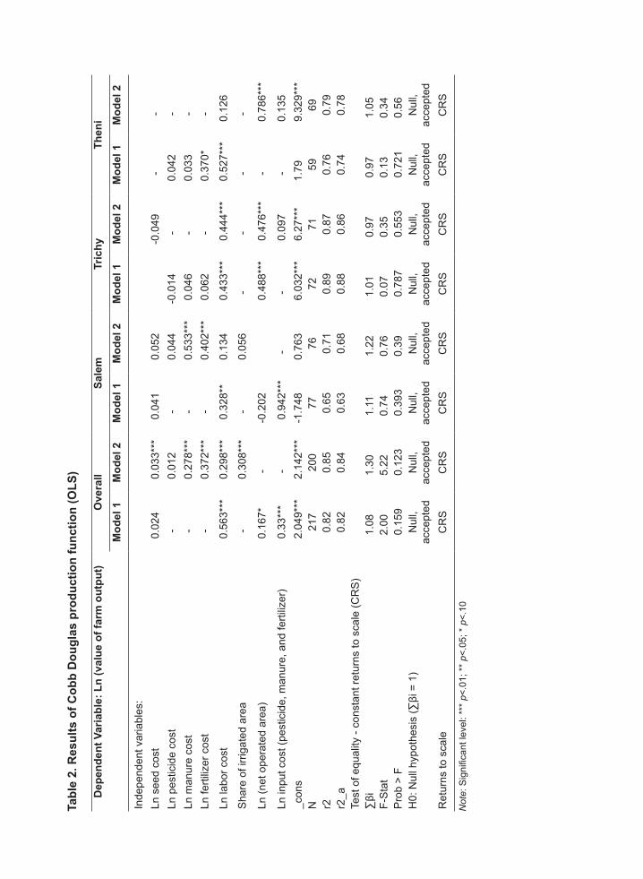
Table 1 shows that the γ-parameter in Cobb-Douglas SFP model proposed by Battese and Corra (1977) explains the variation of output from the frontier attributed to technical inefficiency; it lies between 0 and 1. Coelli (1996) and Coelli and Battese (1996) argue that if γ = 0, it implies that the traditional average response function is an appropriate representation of the data, which can be consistently estimated by average production function (or ordinary least squares [OLS]) methods. To address multicollinearity issues, the study applied two models (i.e., models 1 and 2). In the first model, input costs of pesticides, manure, and fertilizers were combined to avoid collinearity with costs

Asian Journal of Agriculture and Development, Vol. 11, No. 1 83
of seed, labor, and NOA. In the second model, various input costs were treated independently. The resulting coefficients are of the expected signs; most of them are statistically significant, except cost of pesticides.
The results show that estimates of γ-parameter are 0.93 and 0.87 for the Cobb-Douglas SFP models 1 and 2, respectively. These imply the presence of technical inefficiency in the farming activities in the study region. Likelihood ratio test results are 29.05 for model 1 and 14.66 for model 2, which are significant at 1 percent level. These indicate that the technical inefficiency effects are a significant component of the total variability of total crop output. The second null hypothesis is that inefficiency effects are not present in the model (H0: γ=β0= ... β4=0). The coefficients of the frontier model are significantly different from 0 at 1 percent level, indicating that inefficiency effects are present. Therefore, based on the likelihood ratio test results, the first and second null hypotheses are rejected and the stochastic model is accepted. The third null hypothesis is that coefficients of the explanatory variables in the determinants of inefficiency model are significant. This null hypothesis is rejected also, although individual effects of some variables may not be significant.
All three hypotheses of the SFP approach indicate presence of inefficiency. They are stochastic and have particular distributional specification in the model.
Parameter Estimates of Average Cobb-Douglas Production Functions
The parameters of the average Cobb-Douglas production functions were estimated using OLS. The results indicate similarities in the slope parameters across equations of both OLS and SFP method (Table 2). These confirm that the frontier function represents a neutral upward shift of the average production function. All parameter estimates are statistically
significant at 1 percent level, except for cost of pesticides, which is insignificant in all models.
Coelli and Battese (1996) argue that the estimates of parameters of the SFP model need to be discussed in terms of output elasticities evaluated at mean values with respect to various inputs. In agreement, this paper discusses results on the basis of estimates of parameters based on average Cobb-Douglas production functions obtained through OLS method (Table 2). Similar to the SFP approach, two models were estimated using OLS method for the overall scenario, combining all the three districts and also for each district. As mentioned above, these two models were intended to address muliticollinearity problems in the estimates.
Seed
In the overall scenario, the elasticity of mean value of farm output for seed is significant in model 2 only, but the coefficient of seed is far lower (0.033) than the coefficients for other inputs (i.e., manure, 0.278; fertilizer, 0.372; and labor cost, 0.298). Only Trichy obtained a negative sign for the seed coefficient (–0.049). In general, farmers in Trichy cultivate banana. The negative seed coefficient in Trichy implies that if the price of banana seed goes up by a unit, the value of output goes down by 0.049 units. In other words, during agricultural year 2009–2010, holding constant the other input variables, a 1 percent increase in seed cost would decrease the output value by about 0.049 percent. In Salem, the coefficient of seed is positive but insignificant, implying that the cost of seeds is not an important factor for the farmers in influencing value of output. The variation in cost of seeds across households is relatively low, resulting in positive but insignificant relationship with the output value.
Land (NOA)
The coefficient of land is positive and significant, indicating that, holding other input

Table 1. Results of Cobb Douglas SFP function based on normal distribution
Dependent Variable: Ln (Value of Farm Output) Model 1 Model 2
Independent variables:Ln seed cost –.017 0.020*Ln pesticide cost - 0.004Ln manure cost - 0.238***Ln fertilizer cost - 0.308***Ln labor cost 0.486*** 0.324***Share of irrigated area - 0.193*Ln NOA 0.313*** -Ln input cost (pesticide, manure, and fertilizer) 0.212*** -_cons 4.982*** 3.650***lnsig2v_cons –.727*** –.351***lnsig2u_cons –.089 –.482**
StatisticsN 217 200sigma_v 0.256 0.309sigma_u 0.956 0.786sigma2 0.980 0.713Lambda 3.738 2.546γ-parameter =(σ_u^2)/σ^2 0.93 0.87Likelihood-ratio test of sigma_u=0: chi2(01) 29.05*** 14.66***
Test of Hypotheses1. Inefficiency effects are not present, H0: γ = β0 = … =βn = 0
Null, rejected Null, rejected
Decision Presence of inefficiency; proceed to TE through
frontier estimates
Presence of inefficiency; proceed to TE through
frontier estimates2. Inefficiency effects are not stochastic, H0:
γ=0 (based on Chi2 stat)
Null, rejected Null, rejected
Decision Inefficiency effects are stochastic
Inefficiency effects are stochastic
Note: Significant level: *** p<.01; ** p<.05; * p<.10; Ln: natural log
Tabl
e 2.
Res
ults
of C
obb
Dou
glas
pro
duct
ion
func
tion
(OLS
)
Dep
ende
nt V
aria
ble:
Ln
(val
ue o
f far
m o
utpu
t)O
vera
llSa
lem
Tric
hyTh
eni
Mod
el 1
Mod
el 2
Mod
el 1
Mod
el 2
Mod
el 1
Mod
el 2
Mod
el 1
Mod
el 2
Inde
pend
ent v
aria
bles
:Ln
see
d co
st0.
024
0.03
3***
0.04
10.
052
-0
.049
--
Ln p
estic
ide
cost
-0.
012
-0.
044
-0.0
14-
0.04
2-
Ln m
anur
e co
st-
0.27
8***
-0.
533*
**0.
046
-0.
033
-Ln
ferti
lizer
cos
t-
0.37
2***
-0.
402*
**0.
062
-0.
370*
-
Ln la
bor c
ost
0.56
3***
0.29
8***
0.32
8**
0.13
40.
433*
**0.
444*
**0.
527*
**0.
126
Sha
re o
f irr
igat
ed a
rea
-0.
308*
**-
0.05
6-
--
-
Ln (n
et o
pera
ted
area
) 0.
167*
--0
.202
0.
488*
**0.
476*
**-
0.78
6***
Ln in
put c
ost (
pest
icid
e, m
anur
e, a
nd fe
rtiliz
er)
0.33
***
-0.
942*
**-
-0.
097
-0.
135
_con
s2.
049*
**2.
142*
**-1
.748
0.76
36.
032*
**6.
27**
*1.
799.
329*
**N
217
200
7776
7271
5969
r20.
820.
850.
650.
710.
890.
870.
760.
79r2
_a0.
820.
840.
630.
680.
880.
860.
740.
78Te
st o
f equ
ality
- co
nsta
nt re
turn
s to
sca
le (C
RS
)∑
βi1.
081.
301.
111.
221.
010.
970.
971.
05F-
Sta
t2.
005.
220.
740.
760.
070.
350.
130.
34P
rob
> F
0.15
90.
123
0.39
30.
390.
787
0.55
30.
721
0.56
H0:
Nul
l hyp
othe
sis
(∑βi
= 1
)N
ull,
acce
pted
N
ull,
acce
pted
N
ull,
acce
pted
N
ull,
acce
pted
N
ull,
acce
pted
N
ull,
acce
pted
N
ull,
acce
pted
N
ull,
acce
pted
R
etur
ns to
sca
leC
RS
CR
SC
RS
CR
SC
RS
CR
SC
RS
CR
S
Not
e: S
igni
fican
t lev
el: *
** p
<.01
; **
p<.0
5; *
p<.
10
86 Srinivasulu Rajendran
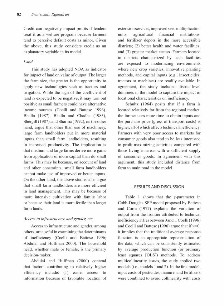
variables constant, 1 percent increase in land size would increase the value of output by about 0.167 percent. In Salem, the elasticity of output for land (NOA) is negative and insignificant, indicating that land size is not affecting the value of output. On the other hand, Theni (0.786) and Trichy (0.476) have very high land elasticity estimates in model 2. The reason is that farmers with large lands in these districts get better returns for their output than those in Salem.
Inputs (Pesticide, Fertilizer, Manure, Tractor Use) and Labor Cost
The machinery variable was dropped due to a large number of zero values in the data. The coefficient of cost of manure, fertilizer, and labor is positive and statistically significant at 1 percent level, suggesting that the value of output can be increased by increasing the expenditure on these inputs. Interestingly, the elasticity for fertilizer is higher than that of the other inputs (i.e., seed, chemicals, land, and labor). In general, the results of model 2 imply that, keeping all other things constant, a 1 percent increase in the cost of fertilizer increases the mean value of output by 0.372 percent. Farmers use fertilizers more intensively than the other inputs, but the coefficient of fertilizer cost varies across districts. Farming is more labor intensive in Trichy and Theni. These districts largely cultivate fruits, which require more labor to harvest. Labor shortage has increased the cost of labor.
Pesticide inputs contributed insignificantly to production. Elasticities for pesticides range from 0.044 in Salem to 0.042 in Theni. The cost of pesticides is lower than those of other inputs such as manure, fertilizer, and labor. The pesticide coefficient is negative and insignificant in Trichy (–0.014). The coefficient of manure shows slight changes, which are insignificant in Trichy and Theni. This indicates that farmers in these districts may be giving
more importance to other inputs. However, manure is an important input in Salem.
In sum, farms with higher input costs and farm size (proxy for capital) could improve production to obtain better value, thereby attaining higher levels of efficiency. The returns-to-scale parameter is 1.08 in model 1 and 1.30 in model 2. In the test for equality, the null hypothesis was accepted, hence the presence of constant returns to scale (CRS) in all models (Table 2). All three districts have CRS, which means a proportionate increase in all the inputs would result in a proportionate increase in output. This indicates that the farmers in all three districts have not been efficiently using their resources.
Technical Efficiency
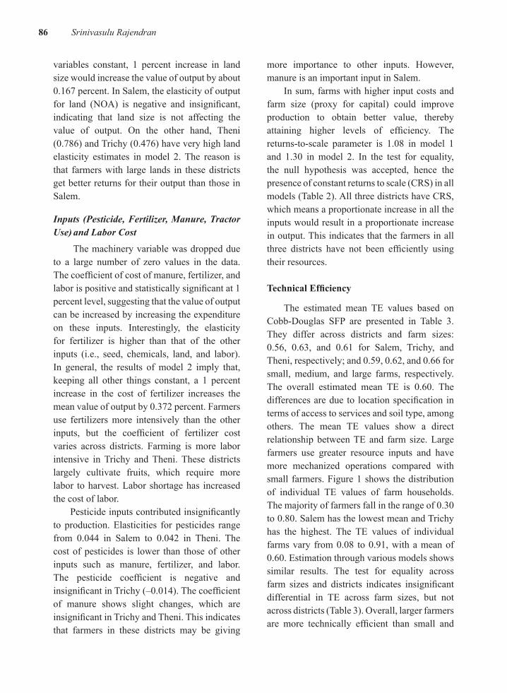
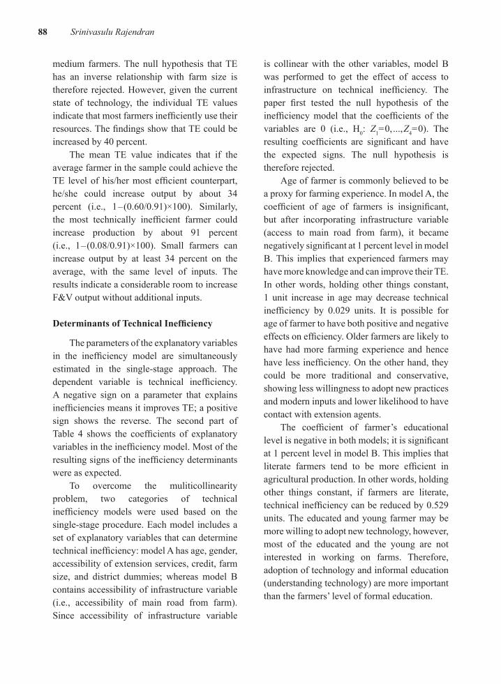
The estimated mean TE values based on Cobb-Douglas SFP are presented in Table 3. They differ across districts and farm sizes: 0.56, 0.63, and 0.61 for Salem, Trichy, and Theni, respectively; and 0.59, 0.62, and 0.66 for small, medium, and large farms, respectively. The overall estimated mean TE is 0.60. The differences are due to location specification in terms of access to services and soil type, among others. The mean TE values show a direct relationship between TE and farm size. Large farmers use greater resource inputs and have more mechanized operations compared with small farmers. Figure 1 shows the distribution of individual TE values of farm households. The majority of farmers fall in the range of 0.30 to 0.80. Salem has the lowest mean and Trichy has the highest. The TE values of individual farms vary from 0.08 to 0.91, with a mean of 0.60. Estimation through various models shows similar results. The test for equality across farm sizes and districts indicates insignificant differential in TE across farm sizes, but not across districts (Table 3). Overall, larger farmers are more technically efficient than small and
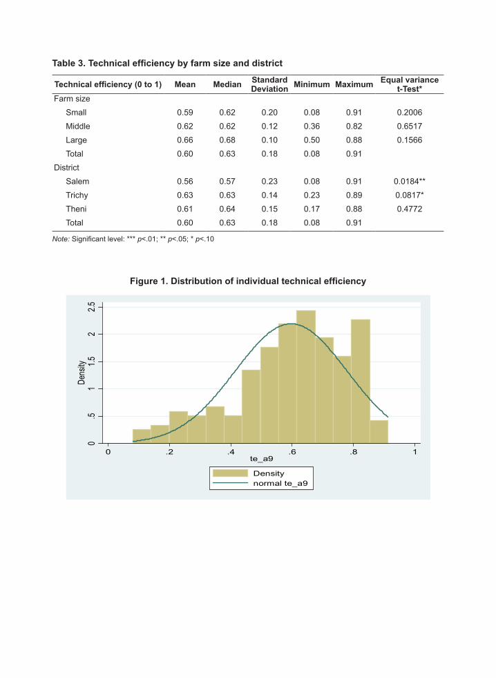
Table 3. Technical efficiency by farm size and district
Technical efficiency (0 to 1) Mean Median Standard Deviation Minimum Maximum Equal variance
t-Test*Farm size
Small 0.59 0.62 0.20 0.08 0.91 0.2006
Middle 0.62 0.62 0.12 0.36 0.82 0.6517
Large 0.66 0.68 0.10 0.50 0.88 0.1566
Total 0.60 0.63 0.18 0.08 0.91
District
Salem 0.56 0.57 0.23 0.08 0.91 0.0184**
Trichy 0.63 0.63 0.14 0.23 0.89 0.0817*
Theni 0.61 0.64 0.15 0.17 0.88 0.4772
Total 0.60 0.63 0.18 0.08 0.91
Note: Significant level: *** p<.01; ** p<.05; * p<.10
Figure 1. Distribution of individual technical efficiency
0.5
11.5
22.5
Dens
ity
0 .2 .4 .6 .8 1te_a9
Densitynormal te_a9
88 Srinivasulu Rajendran
medium farmers. The null hypothesis that TE has an inverse relationship with farm size is therefore rejected. However, given the current state of technology, the individual TE values indicate that most farmers inefficiently use their resources. The findings show that TE could be increased by 40 percent.
The mean TE value indicates that if the average farmer in the sample could achieve the TE level of his/her most efficient counterpart, he/she could increase output by about 34 percent (i.e., 1 – (0.60/0.91)×100). Similarly, the most technically inefficient farmer could increase production by about 91 percent (i.e., 1 – (0.08/0.91)×100). Small farmers can increase output by at least 34 percent on the average, with the same level of inputs. The results indicate a considerable room to increase F&V output without additional inputs.
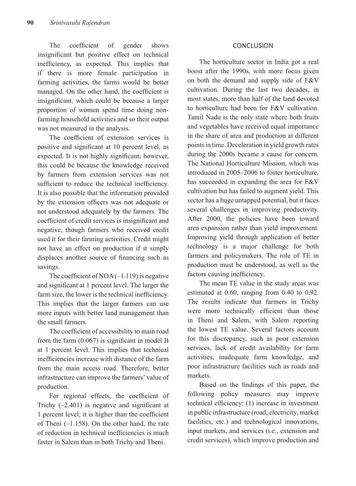
Determinants of Technical Inefficiency
The parameters of the explanatory variables in the inefficiency model are simultaneously estimated in the single-stage approach. The dependent variable is technical inefficiency. A negative sign on a parameter that explains inefficiencies means it improves TE; a positive sign shows the reverse. The second part of Table 4 shows the coefficients of explanatory variables in the inefficiency model. Most of the resulting signs of the inefficiency determinants were as expected.
To overcome the muliticollinearity problem, two categories of technical inefficiency models were used based on the single-stage procedure. Each model includes a set of explanatory variables that can determine technical inefficiency: model A has age, gender, accessibility of extension services, credit, farm size, and district dummies; whereas model B contains accessibility of infrastructure variable (i.e., accessibility of main road from farm). Since accessibility of infrastructure variable
is collinear with the other variables, model B was performed to get the effect of access to infrastructure on technical inefficiency. The paper first tested the null hypothesis of the inefficiency model that the coefficients of the variables are 0 (i.e., H0: Z1= 0, ..., Z4= 0). The resulting coefficients are significant and have the expected signs. The null hypothesis is therefore rejected.
Age of farmer is commonly believed to be a proxy for farming experience. In model A, the coefficient of age of farmers is insignificant, but after incorporating infrastructure variable (access to main road from farm), it became negatively significant at 1 percent level in model B. This implies that experienced farmers may have more knowledge and can improve their TE. In other words, holding other things constant, 1 unit increase in age may decrease technical inefficiency by 0.029 units. It is possible for age of farmer to have both positive and negative effects on efficiency. Older farmers are likely to have had more farming experience and hence have less inefficiency. On the other hand, they could be more traditional and conservative, showing less willingness to adopt new practices and modern inputs and lower likelihood to have contact with extension agents.
The coefficient of farmer’s educational level is negative in both models; it is significant at 1 percent level in model B. This implies that literate farmers tend to be more efficient in agricultural production. In other words, holding other things constant, if farmers are literate, technical inefficiency can be reduced by 0.529 units. The educated and young farmer may be more willing to adopt new technology, however, most of the educated and the young are not interested in working on farms. Therefore, adoption of technology and informal education (understanding technology) are more important than the farmers’ level of formal education.
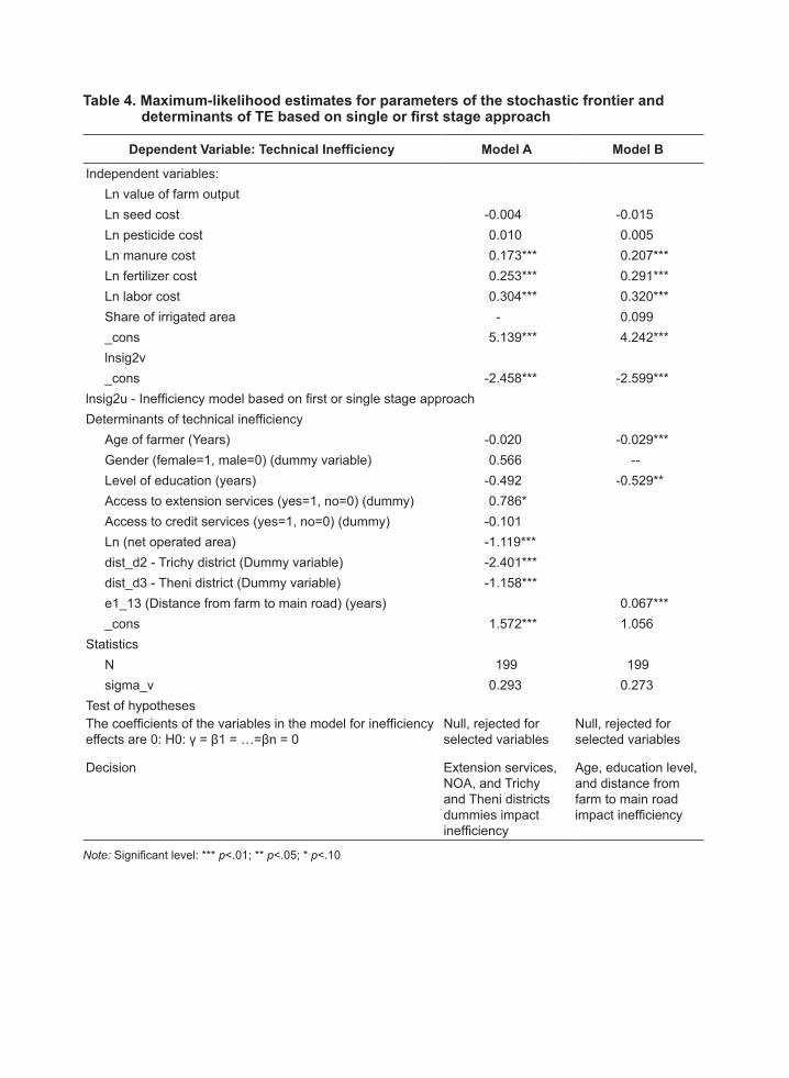
Table 4. Maximum-likelihood estimates for parameters of the stochastic frontier and determinants of TE based on single or first stage approach
Dependent Variable: Technical Inefficiency Model A Model B
Independent variables:Ln value of farm output Ln seed cost -0.004 -0.015Ln pesticide cost 0.010 0.005Ln manure cost 0.173*** 0.207***Ln fertilizer cost 0.253*** 0.291***Ln labor cost 0.304*** 0.320***Share of irrigated area - 0.099_cons 5.139*** 4.242***lnsig2v _cons -2.458*** -2.599***
lnsig2u - Inefficiency model based on first or single stage approachDeterminants of technical inefficiency
Age of farmer (Years) -0.020 -0.029***Gender (female=1, male=0) (dummy variable) 0.566 --Level of education (years) -0.492 -0.529**Access to extension services (yes=1, no=0) (dummy) 0.786* Access to credit services (yes=1, no=0) (dummy) -0.101 Ln (net operated area) -1.119*** dist_d2 - Trichy district (Dummy variable) -2.401*** dist_d3 - Theni district (Dummy variable) -1.158*** e1_13 (Distance from farm to main road) (years) 0.067***_cons 1.572*** 1.056
StatisticsN 199 199sigma_v 0.293 0.273
Test of hypothesesThe coefficients of the variables in the model for inefficiency effects are 0: H0: γ = β1 = …=βn = 0
Null, rejected for selected variables
Null, rejected for selected variables
Decision Extension services, NOA, and Trichy and Theni districts dummies impact inefficiency
Age, education level, and distance from farm to main road impact inefficiency
Note: Significant level: *** p<.01; ** p<.05; * p<.10
90 Srinivasulu Rajendran
The coefficient of gender shows insignificant but positive effect on technical inefficiency, as expected. This implies that if there is more female participation in farming activities, the farms would be better managed. On the other hand, the coefficient is insignificant, which could be because a larger proportion of women spend time doing non-farming household activities and so their output was not measured in the analysis.
The coefficient of extension services is positive and significant at 10 percent level, as expected. It is not highly significant; however, this could be because the knowledge received by farmers from extension services was not sufficient to reduce the technical inefficiency. It is also possible that the information provided by the extension officers was not adequate or not understood adequately by the farmers. The coefficient of credit services is insignificant and negative, though farmers who received credit used it for their farming activities. Credit might not have an effect on production if it simply displaces another source of financing such as savings.
The coefficient of NOA (–1.119) is negative and significant at 1 percent level. The larger the farm size, the lower is the technical inefficiency. This implies that the larger farmers can use more inputs with better land management than the small farmers.
The coefficient of accessibility to main road from the farm (0.067) is significant in model B at 1 percent level. This implies that technical inefficiencies increase with distance of the farm from the main access road. Therefore, better infrastructure can improve the farmers’ value of production.
For regional effects, the coefficient of Trichy (–2.401) is negative and significant at 1 percent level; it is higher than the coefficient of Theni (–1.158). On the other hand, the rate of reduction in technical inefficiencies is much faster in Salem than in both Trichy and Theni.
CONCLUSION
The horticulture sector in India got a real boost after the 1990s, with more focus given on both the demand and supply side of F&V cultivation. During the last two decades, in most states, more than half of the land devoted to horticulture had been for F&V cultivation. Tamil Nadu is the only state where both fruits and vegetables have received equal importance in the share of area and production at different points in time. Deceleration in yield growth rates during the 2000s became a cause for concern. The National Horticulture Mission, which was introduced in 2005–2006 to foster horticulture, has succeeded in expanding the area for F&V cultivation but has failed to augment yield. This sector has a huge untapped potential, but it faces several challenges in improving productivity. After 2000, the policies have been toward area expansion rather than yield improvement. Improving yield through application of better technology is a major challenge for both farmers and policymakers. The role of TE in production must be understood, as well as the factors causing inefficiency.
The mean TE value in the study areas was estimated at 0.60, ranging from 0.40 to 0.92. The results indicate that farmers in Trichy were more technically efficient than those in Theni and Salem, with Salem reporting the lowest TE value. Several factors account for this discrepancy, such as poor extension services, lack of credit availability for farm activities, inadequate farm knowledge, and poor infrastructure facilities such as roads and markets.
Based on the findings of this paper, the following policy measures may improve technical efficiency: (1) increase in investment in public infrastructure (road, electricity, market facilities, etc.) and technological innovations, input markets, and services (i.e., extension and credit services), which improve production and
Asian Journal of Agriculture and Development, Vol. 11, No. 1 91
marketing efficiency; (2) implementation of cluster farming system among small farmers, where knowledge sharing can be encouraged, since farm size is directly related to TE; and (3) provision of better incentives for farm laborers, such as a competitive pay package based on market price or linking national and state employment programs with farming activities in the study area. This is to address the labor shortage in the region, which pushes up the labor cost (wage rate); this is a particular concern in F&V production, which is labor intensive.
REFERENCES
Abdulai, Awudu, and H. Tietje. 2007. “Estimating Technical Efficiency under Unobserved Heterogeneity with Stochastic Frontier Models: Application to Northern German Dairy Farms.” European Review of Agricultural Economics 34 (3): 393–416.
Abdulai, Awudu, and Wallace Huffman. 2000. “Structural Adjustment and Economic Efficiency of Rice Farmers in Northern Ghana.” Economic Development and Cultural Change 48 (3): 503–520.
Aigner, D.J., C.A.K. Lovell, and P. Schmidt. 1977. “Formulation and Estimation of Stochastic Frontier Production Function Models.” Journal of Econometrics 6 (1): 21–37.
Ali, M., and M.A. Choudhry. 1990. “Inter-regional Farm Efficiency in Pakistan’s Punjab: A Frontier Production Function Study.” Journal of Agricultural Economics 41 (1): 62–74.
Asogwa, B.C., J.C. Ihemeje, and J.A.C. Ezihe. 2011. “Technical and Allocative Efficiency Analysis of Nigerian Rural Farmers: Implication for Poverty Reduction.” Agricultural Journal 6 (5): 243–251.
Battese, G.E., and T.J. Coelli. 1995. “A Model for Technical Inefficiency Effects in Stochastic Frontier Production Functions for Panel Data.” Empirical Economics 20 (2): 325–332.
Battese, G.E., and G.S. Corra. 1977. “Estimation of a Production Frontier Model: With Application to the Pastoral Zone of Eastern Australia.” Australian Journal of Agricultural Economics 21 (3): 169–179.
Battese, G.E., and G.A. Tessema. 1993. “Estimation of Stochastic Frontier Production Functions with Time-varying Parameters and Technical Efficiencies Using Panel Data from Indian Villages.” Agricultural Economics 9 (4): 313–333.
Bhalla, Sheila. 1987. Trends in Employment in Indian Agriculture, Land and Asset Distribution. New Delhi: Indian Society of Agricultural Economics.
Bhalla, G.S., and G.K. Chadha. 1983. The Green Revolution and the Small Peasant: A Study of Income Distribution among Punjab Cultivators. New Delhi: Concept Publishing Company.
Birthal, Pratap Singh, P.K. Joshi, Sonia Chauhan, and Harvinder Singh. 2008. “Can Horticulture Revitalise Agricultural Growth?” Indian Journal of Agricultural Economics 63 (3): 310.
Birthal, Pratap Singh, Pramod Kumar Joshi, Devesh Roy, and Amit Thorat. 2012. “Diversification in Indian Agriculture toward High-value Crops: The Role of Small Farmers.” Canadian Journal of Agricultural Economics 61 (1): 61–91.
Bravo-Ureta, B.E., and A.E. Pinheiro. 1997. “Technical, Economic and Allocative Efficiency in Peasant Farming: Evidence from the Dominican Republic.” The Developing Economies 35 (1): 48–67.
Chand, Ramesh, S.S. Raju, and L.M. Pandey. 2008. “Progress and Potential of Horticulture in India.” Indian Journal of Agricultural Economics 63(3): 299–309.
Coelli, T.J. 1996. “Measurement of Total Factor Productivity Growth and Biases in Technological Change in Western Australian Agriculture.” Journal of Applied Econometrics 11 (1): 77–91.
Coelli, T.J., and G.E. Battese. 1996. “Identification of Factors which Influence the Technical Inefficiency of Indian Farmers.” Australian Journal of Agricultural Economics 40 (2): 103–128.
CSO (Central Statistical Organization). 2012. Statewise and Cropwise Estimates of Value of Output from Agriculture (1980-2009). New Delhi: Central Statistical Organization, Ministry of Statistics and Programme Implementation, Government of India.
Debreu, G. 1951. “The Coefficient of Resource Utilization.” Econometrica 19 (3): 273–292.
92 Srinivasulu Rajendran
FAO (Food and Agriculture Organization). 2012. Food and Agriculture Organization Statistics. Rome, Italy: Food and Agriculture Organization of the United Nations.
Farrell, M.J. 1957. “The Measurement of Productive Efficiency.” Journal of the Royal Statistical Society 120 (3): 253–281.
Huffman, W.E. 1974. “Decision Making: The Role of Education.” American Journal of Agricultural Economics 56 (1): 85–97.
Iraizoz B., M. Rapun, and I. Zabaleta. 2003. “Assessing Technical Efficiency of Horticultural Production in Navarra, Spain.” Agricultural Systems 78 (3): 387–403.
Joshi, P.K., Laxmi Tewari, and P.S. Birthal. 2006. “Diversification and its Impact on Smallholders: Evidence from a Study on Vegetable Production.” Agricultural Economics Research Review 19 (2): 219–236.
Kalirajan, K.P., and R.T. Shand. 1999. “Frontier Production Functions and Technical Efficiency Measures.” Journal of Economic Surveys 13 (2): 149–172.
Kumar, Praduman. 1998. “Food Demand and Supply Projections for India.” Agricultural Economics Policy Paper 98-01. New Delhi: Indian Agricultural Research Institute.
Kumar, Parmod, and Sandip Sarkar. 2012. Economic Reforms and Small Farms: Implications for Production, Marketing and Employment. New Delhi: Academic Foundation and Institute for Human Development.
Kumbhakar, S.C. 1994. “Efficiency Estimation in a Profit Maximizing Model Using Flexible Production Function.” Agricultural Economics 10 (2): 143–152.
Kumar, Praduman, and V.C. Mathur. 1996. “Structural Changes in Demand for Food in India.” Indian Journal of Agricultural Economics 51 (4): 664–673.
Lockheed, M.E., D.T. Jamison, and L.J. Lau. 1980. “Farmer Education and Farm Efficiency: A Survey.” Economic Development and Cultural Change 29 (1): 37–76.
McCarty, T.A., and S. Yaisawarng. 1993. “Technical Efficiency in New Jersey School Districts.” In The Measurement of Productive Efficiency: Techniques and Applications, edited by H.O. Fried and S.S. Schmidt, 271–287. U.K.: Oxford.
Meeusen, W., and J. Van den Broeck. 1977. “Efficiency Estimation from Cobb-Douglas Production Functions with Composed Error.” International Economic Review 18: 435–444.
Mittal, Surabhi. 2007. “Can Horticulture Be a Success Story for India?” Working Paper No. 197. New Delhi: ICRIER.
MoA (Ministry of Agriculture). 2011. Land Use Statistics at a Glance 2010. New Delhi: Directorate of Economics and Statistics, Ministry of Agriculture, Government of India.
Parikh, A., F. Ali, and M. K. Shah. 1995. “Measurement of Economic Efficiency in Pakistani Agriculture.” American Journal of Agricultural Economics 77 (3): 675–685.
Ram, Rati. 1980. “Role of Education in Production: A Slightly New Approach.” Quarterly Journal of Economics 95 (2): 365–373.
Schultz, Theodore W. 1964. Transforming Traditional Agriculture. New Haven, CT: Yale University Press.
Seyoum, E.T., G.E. Battese, and E.M. Fleming. 1998. “Technical Efficiency and Productivity of Maize Producers in Eastern Ethiopia: A Study of Farmers within and outside the Sasakawa-Global 2000 Project.” Agricultural Economics 19 (3): 341–348.
Sharma, R.K. 1992. Technical Change, Income Distribution and Rural Poverty: A Case Study of Haryana. Delhi: Shipra Publications.
Shergill, H.S. 1987. “Impact of New Technology on Farm Size Productivity Relationship in Punjab Agriculture: A Decomposition Analysis.” Department of Economics, Punjab University, Chandigarh. (mimeo)
Singh, H.P, Prem Nath, O. P Dutta, and M. Sudha. 2004. Horticulture Development, State of the Indian Farmer: A Millennium Study. New Delhi: Academic Foundation, Ministry of Agriculture, Government of India.
Villano, R., and E. Fleming. 2004. “Analysis of Technical Efficiency in a Rain-fed Lowland Rice Environment in Central Luzon, Philippines Using a Stochastic Frontier Production Function with Heteroskedastic Error Structure.” Working Paper Series in Agricultural and Resource Economics No. 2004-15. University of New England, Armidale.
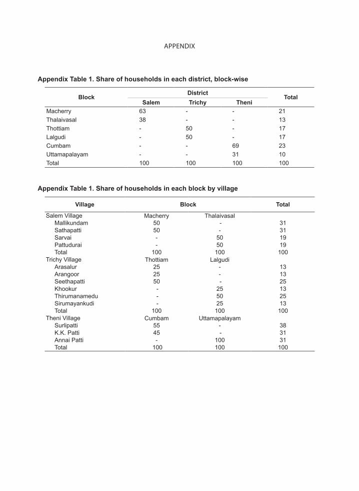
APPENDIX
Appendix Table 1. Share of households in each district, block-wise
Block District
TotalSalem Trichy Theni
Macherry 63 - - 21Thalaivasal 38 - - 13Thottiam - 50 - 17Lalgudi - 50 - 17Cumbam - - 69 23Uttamapalayam - - 31 10Total 100 100 100 100
Appendix Table 1. Share of households in each block by village
Village Block Total
Salem Village Macherry ThalaivasalMallikundam 50 - 31Sathapatti 50 - 31Sarvai - 50 19Pattudurai - 50 19Total 100 100 100
Trichy Village Thottiam LalgudiArasalur 25 - 13Arangoor 25 - 13Seethapatti 50 - 25Khookur - 25 13Thirumanamedu - 50 25Sirumayankudi - 25 13Total 100 100 100
Theni Village Cumbam UttamapalayamSurlipatti 55 - 38K.K. Patti 45 - 31Annai Patti - 100 31Total 100 100 100