Technical Commentary on FM3-34.343, Military Nonstandard

1_ CO

15 o >* ■■■■

c ^ 1

o o (0

K"^K^

o 0

o n

CO O -I

>'!'

US Army Corps of Engineers® Engineer Research and Development Center

Technical Commentary on FM3-34.343, "Military Nonstandard Fixed Bridging"

James C. Ray and Yazmin Seda-Sanabria August 2002

Approved for public release; distribution is unlimited. (K

7 b' X

^

The contents of this report are not to be used for advertising, publication, or promotional purposes. Citation of trade names does not constitute an official endorsement or approval of the use of such commercial products.

The findings of this report are not to be construed as an official Department of the Army position, unless so designated by other authorized documents.

$ PRINTED ON RECYCLED PAPER

ERDC/GSLTR-02-15 August 2002

Technical Commentary on FM3-34.343, "Military Nonstandard Fixed Bridging"

by James C. Ray, Yazmin Seda-Sanabria Geotechnical and Structures Laboratory U.S. Army Engineer Research and Development Center 3909 Halls Ferry Road Vicksburg, MS 39180-6199

Final report

Approved for public release; distribution is unlimited

Prepared for U.S. Army Corps of Engineers Washington, DC 20314-1000

Contents

Preface vii

Conversion Factors, Non-SI to SI Units of Measurement viii

1—Introduction 1

2—Commentary on Chapter 3, Classification 2

Correlation-Curve Classification 2 Introduction; paragraphs 3-9 though 3-13 2 Truss and suspension bridge span lengths; paragraph 3-14 2 Correlation curve uses; paragraphs 3-15 through 3-18 3

Analytical Bridge Classification 5 Controlling features; paragraphs 3-22 through 3-25 5 Live load; paragraph 3-30 5 Impact load; paragraph 3-31 6 Load distribution; paragraph 3-32 6 Allowable stresses; paragraph 3-33 7 Equivalent span length; paragraph 3-41 7

Solid-Sawn and Glue-Laminated Timber-Stringer Bridges 8 Allowable stresses; paragraph 3-46 8 Applied dead load shear per stringer; paragraph 3-52 9 Total live-load shear for one or two lanes; paragraph 3-54 10 Tracked vehicles on glue-laminated stringer bridges; paragraph 3-55 11 Plank decking; paragraph 3-58 12 Laminated decking; paragraph 3-59 12

Steel-Stringer Bridges 13 Yield and allowable stresses; paragraph 3-63 13 Stringer moment-classification procedure; paragraph 3-64 14

Composite-Stringer Bridges 15 Stringer section modulus; paragraph 3-72 15 Effective concrete- and steel flange widths; paragraphs 3-73 and 3-74 15

Steel-Girder Bridges 16 Effective number of girders for one- and two-lane traffic; paragraphs 3-83 and 3-84 16

Stringer shear classification; paragraph 3-93 19 Maximum allowable floor beam reactions; paragraph 3-98 21 Floor beam shear classification; paragraph 3-100 22 Maximum allowable floor beam reactions; paragraph 3-104 23 Special allowance for caution crossing; paragraph 3-105 23 Maximum floor beam reactions; figures 3-21 through 3-24 24

Truss Bridges 30 Expedient classification; paragraph 3-113 30 Total dead load; paragraph 3-115 30 Compressive force in top chord; paragraph 3-120 30

Reinforced Concrete Slab Bridges 30 Assumptions; paragraph 3-131 30 Concrete and reinforcing steel strengths; paragraphs 3-132 and 3-133 31 Compressive stress block depth; paragraph 3-135 31 Slab moment capacity; paragraph 3-136 31 Allowable live load moment; paragraph 3-138 31 Effective slab width; paragraph 3-139 32

Reinforced Concrete T-Beam Bridges 32 Assumptions; paragraph 3-143 32 Moment capacity; paragraphs 3-145 through 3-148 32

Prestressed Concrete Bridges 32 Analytical classification; paragraph 163 32 Moment capacity; paragraphs 3-164 through 3-174 33

Arch Bridges 33 Modern arch bridge; paragraph 3-179 33 Masonry arch bridge; paragraphs 3-180 through 3-183 33

-Commentary on Chapter 6, Design of Bridge Superstructures 34

Deck Design 34 Effective span length; paragraphs 6-10 through 6-13 34 Required plank deck thickness; paragraph 6-16 35 Reinforced concrete deck; paragraph 6-21 36 Slab dimensions; paragraph 6-24 37 Wearing surface; paragraph 6-25 37 Dead load; paragraph 6-26 37 Live load; paragraph 6-28 38 Required nominal strength; paragraph 6-29 39 Reinforcing steel ratio; paragraph 6-30 40 Strength coefficient of resistance; paragraph 6-31 43 Effective depth; paragraph 6-32 44 Revised reinforcing steel ratio; paragraph 6-34 46 Bar selection and placement; paragraph 6-35 47

IV

Stringer Design 47 Live load moment; paragraph 6-51 47 Allowable stresses; paragraphs 6-53 through 6-55 47 Vertical deflection check; paragraph 6-58 48 Maximum allowable unbraced length; paragraph 6-64 50 Design live load shear per stringer; paragraph 6-85 50

References 51

SF298

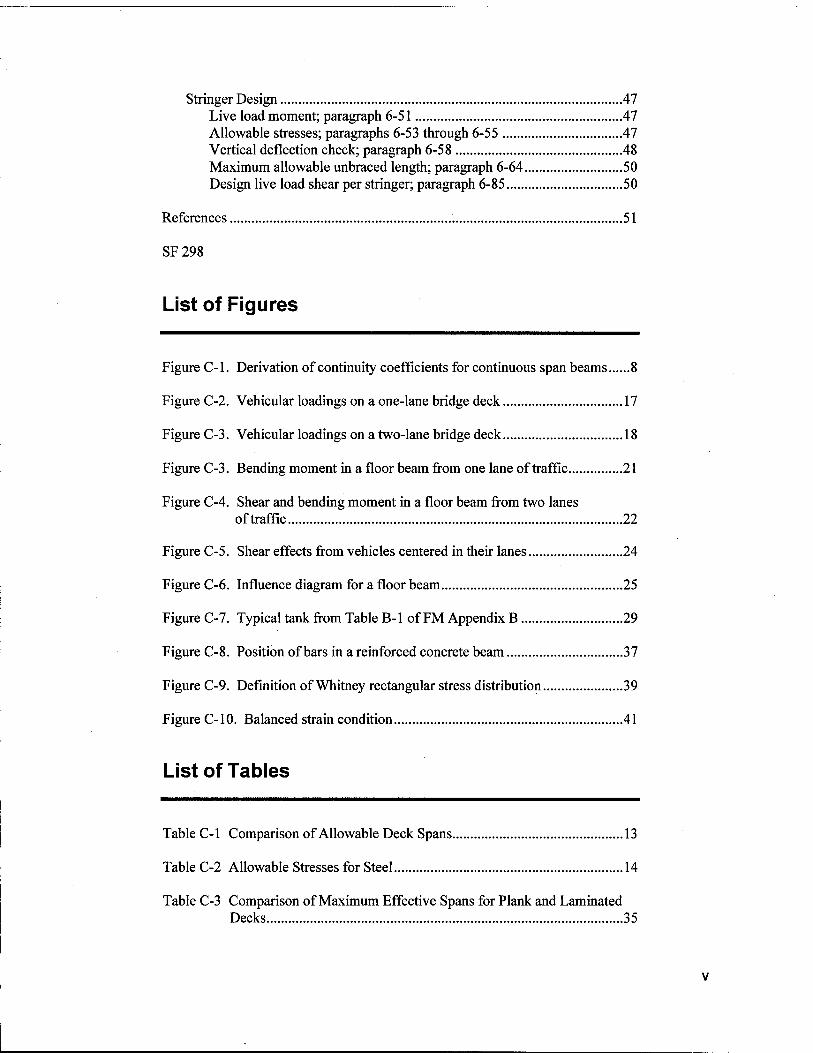
List of Figures

Figure C-l. Derivation of continuity coefficients for continuous span beams 8

Figure C-2. Vehicular loadings on a one-lane bridge deck 17

Figure C-3. Vehicular loadings on a two-lane bridge deck 18

Figure C-3. Bending moment in a floor beam from one lane of traffic 21

Figure C-4. Shear and bending moment in a floor beam from two lanes of traffic ....22

Figure C-5. Shear effects from vehicles centered in their lanes 24

Figure C-6. Influence diagram for a floor beam 25

Figure C-7. Typical tank from Table B-l of FM Appendix B 29

Figure C-8. Position of bars in a reinforced concrete beam 37

Figure C-9. Definition of Whitney rectangular stress distribution 39

Figure C-10. Balanced strain condition 41

List of Tables

Table C-l Comparison of Allowable Deck Spans 13

Table C-2 Allowable Stresses for Steel 14

Table C-3 Comparison of Maximum Effective Spans for Plank and Laminated Decks 35

Table C-4. Maximum Reinforcement Steel Ratio 42

Table C-5. Reinforcement Steel Ratio 42

VI

Preface

The study was part of the Department of the Army Project No. 4A162784AT40, Work Package 159B, "Bridge Assessment and Repair," Work Unit BR001, "Assessment," which was sponsored by Headquarters, U.S. Army Corps of Engineers.

The work was accomplished at the U.S. Army Engineer Research and Development Center (ERDC), Vicksburg, MS, under the general supervision of Dr. David W. Pittman, Acting Director, Geotechnical and Structures Laboratory (GSL), Dr. Robert L. Hall, Chief, Geosciences and Structures Division (GSD), GSL; and Mr. James S. Shore, Chief, Structural Engineering Branch (StEB), GSL. This report was prepared by Mr. James C. Ray and Ms. Yazmin Seda- Sanabria, GSL. Ms. Corine E. Pugh, Graphics Specialist, DynCorp Corporation, Vicksburg, assisted the authors in the preparation of this report.

At the time of this report, the Director of the ERDC was Dr. James R. Houston, and the Commander and Executive Director was COL John W. Morris III, EN.

The contents of this report are not to be used for advertising, publication or promotional purposes. Citation of trade names does not constitute an official endorsement or approval of the use of such commercial products.

VII

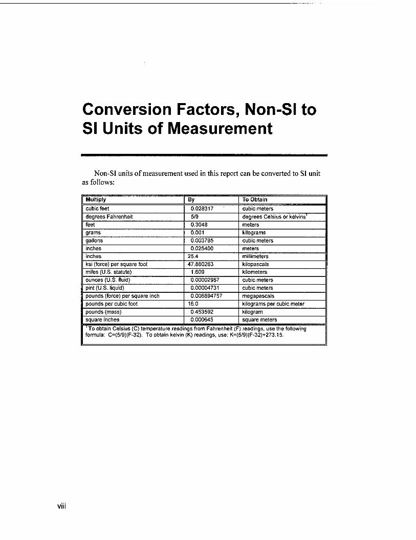
Conversion Factors, Non-SI to SI Units of Measurement

Non-SI units of measurement used in this report can be converted to SI unit as follows:

Multiply By To Obtain

cubic feet 0.028317 cubic meters

degrees Fahrenheit 5/9 degrees Celsius or kelvins1

feet 0.3048 meters

grams 0.001 kilograms gallons 0.003785 cubic meters

inches 0.025400 meters inches 25.4 millimeters ksi (force) per square foot 47.880263 kilopascals miles (U.S. statute) 1.609 kilometers ounces (U.S. fluid) 0.00002957 cubic meters

pint (U.S. liquid) 0.00004731 cubic meters pounds (force) per square inch 0.006894757 megapascals

pounds per cubic foot 16.0 kilograms per cubic meter

pounds (mass) 0.453592 kilogram square inches 0.000645 square meters 1 To obtain Celsius (C) temperature readings from Fahrenheit (F) readings, use the following formula: C=(5/9)(F-32). To obtain kelvin (K) readings, use: K=(5/9)(F-32)+273.15.

VIII

1 Introduction

The newly revised Army field manual, FM 3-34.343, "Military Nonstandard Fixed Bridging," was published by Headquarters, Department of the Army, on 12 February 2002. The FM 3-34.343 superceded the old FM 5-446 of the same title, dated 3 June 1991.

Past editions of Technical and Field Manuals for the military have had no documentation or references by which the content could be verified or checked. In an effort to alleviate this problem, the U.S. Army Engineer Research and Development Center (ERDC) has prepared this technical commentary on Chapter 3, "Classification," and Chapter 6, "Design of Bridge Superstructures." The authors of this report (Mr. James C. Ray and Ms. Yazmin Seda-Sanabria) were uniquely qualified to prepare the commentary to Chapters 3 and 6 as they were primary authors and technical editors of these chapters within the FM 3-34.343. A commentary of this type is essential as military engineering field manuals contain numerous simplifying assumptions and behind-the-scenes derivations that are not obvious to the user unless carefully explained. The reader is advised to read the following paragraph carefully as use of this report in conjunction with the FM is explained:

Discussion and References have been provided herein for all of the assumptions made in the development of Chapters 3 and 6. This commentary must be used in conjunction with a copy of the FM 3-34.343 (referred to hereafter as FM) as it directly references, but does not repeat specific paragraph titles/numbers and equation numbers. Paragraph titles herein have been made to correspond to those in the FM. Only those paragraphs requiring more in-depth elaboration are discussed in this report. Derivations have been provided for all equations except for those which are just basic structural mechanics. Numbers for figures, tables, and equations that are only contained within this Commentary are preceded by a "C" to set them apart from those referenced in the FM. Those that are also part of the FM are given the same number as in FM.

Chapter 1 Introduction

2 Commentary on Chapter 3, Classification

Correlation-Curve Classification

Introduction; paragraphs 3-9 through 3-13

These curves have been greatly misunderstood in the past. Many engineers find it difficult to believe that an in-depth analytical bridge rating can be replaced by a simple set of curves. Of course, they cannot. These curves do, however, provide a very good estimate of military load classification (MLC) in many cases. The validity of this method depends on the following factors: (1) The bridge must have been originally designed using the proper design loadings and proper guidelines and criteria. For most bridges in developed countries, this will be the case. (2) The curves are derived by calculating the midspan bending moment caused by the civilian design vehicle and correlating it to the military vehicle, which causes the same amount of moment. Based on this, it would seem that the Correlation Curves would only be applicable to bridges where midspan bending moment is the limiting criteria (i.e. the weakest link). However, this is not actually the case. If it is assumed that the longitudinal members will carry the applied bending moment, then it can also be assumed that all other members (i.e. decks, floor beams, connections, etc.) were designed properly (in shear and moment) for at least the same size vehicle. Therefore, the Correlation Curves could just as easily be based on this criteria. (3) If the bridge was originally designed for two-way civilian traffic, then a two-way MLC is obtained from the curves by default. If a one-way MLC (as required for Caution Crossings) is desired, the appropriate correction factor (discussed below) from Table 3-1 can be applied to the military live load moment prior to going to the moment tables in FM Appendix C. Or, if the bridge was originally designed as one-way bridge, then the resulting MLC will also be a one-way MLC. A two-way MLC cannot be obtained from a bridge originally designed as a one-way bridge.

Truss and suspension bridge span lengths; paragraph 3-14

For truss and suspension bridges, two span lengths must be considered: the overall length of the main span and the length of one of the panels; i.e. support points for floor system. This is required since these bridges may be of very long span and would thus have been designed for a "train" of closely-spaced civilian

Chapter 2 Commentary on Chapter 3, Classification

trucks. Correlation of this design loading to that produced by a convoy of 100-ft1

spaced military vehicles (standard convoy spacing) could likely produce a high allowable military loading. However, the floor system will only be designed for a singular civilian truck, which would correlate to a lower military truck loading. To address this possibility, it is necessary to consider both span lengths in the correlation and take the lower resulting MLC.

Correlation curve uses; paragraphs 3-15 through 3-18

As mentioned above, the curves are derived by correlating the maximum midspan longitudinal bending moment from the civilian design vehicle to the military vehicle(s) that produce the same amount of longitudinal bending moment. The beam size, defined by its section modulus (S), can be directly related to the total applied bending moment as follows:

s = J^+mJtrl) (ci)

Fb,DL Fb,LL

where:

S = Stringer section modulus, mDL = Bending moment due to the dead load weight of the bridge

superstructure, mLL - Bending moment due to the vehicular live load,

FbDL = Portion of allowable bending stress utilized for carrying the dead load,

FbDL = Portion of allowable bending stress utilized for carrying the live load,

I = Live load impact factor.

The section modulus is an intrinsic property of the stringer cross-sectional shape and does not depend on the specific analysis approach used. Therefore, the section modulus is a relatable term between civilian and military bridge rating methods. In addition, it can be reasonably assumed that the contributions due to the dead load moment are the same, regardless of the analytical method, and can thus be cancelled out of the equation. Relating the section modulus equation between military and civilian analyses gives:

Military S = Civilian S

F F ( b,mil b,civ

Solving this relationship for the military bending moment as a function of the civilian bending moment yields:

1 A table for converting Non-SI units of measurement to SI units appears on page viii.


m LL,mil

V b, mil

F \ b,civ ) / + '■mil J

m LL,civ (C-3)

The following relationships are generally used in military and civilian analyses:

b, mil y'

F, . =0.55F , b,civ y'

I ., =0.15 for steel and concrete bridges,

50 / . civ Z + 125

where:

Fy = the yield stress of steel, and

L = the span length.

Substitution of these values into Equation C-3 yields:

m LL,mil 0.8

0.55

1 + 50 A Z.+125

1.15 m LL.civ (C-4)

Equation C-4 was used to plot the Correlation Curves shown in the FM Fig- ure 3-1. The civilian live load moments (as a function of span length) were taken from precalculated tables in Reference 1.

The U.S. Correlation Curves in the original TM5-312 (Reference 8) and the FM5-446 (Reference 9) had an inset of curves designed to give a "lateral distribution" correction factor to the military live load moment. These curves were derived because the military distribution factors were calculated differently than the standard civilian distribution factors (Reference 1) and to facilitate conversion from the civilian two-way loading to a military one-way loading (as required for caution crossings). In the new FM 3-34.343, the civilian distribution factors have been adopted in place of the original military distribution factors (See discussion of Paragraph 3-21 through 3-26 below). Therefore, the set of inset correction curves is no longer required. However, a means to convert the civilian two-way MLC to a one-way MLC is still required. This is accomplished by applying the factors from Table 3-1 to the live load moment obtained from Figure 3-1 prior to entering the military moment tables in FM Appendix B. These correction factors are simply the ratio of the two-way distribution factor to the one-way factor for each deck type in Table 3-3.

The Correlation Curves for foreign countries were derived in the same manner as described above, using the standard civilian design vehicles for each of those countries. These curves were extracted directly from Reference 8 and have not been checked or validated. Future work in this area should be directed toward a verification/update of these curves. Note that the Y-axis provides the MLC without having to use the Moment Tables in FM Appendix B. Also, note


that the values provided are for two-way traffic. In order to obtain a one-way caution crossing MLC, multiply the two-way value by the appropriate correction factor from Table 3-1.

Analytical Bridge Classification

Controlling features; paragraphs 3-22 through 3-25

The assumption that the bridge superstructure beams will always control the rating is not unusual. This is standard policy of the American Association of State Highway and Transportation Officials (AASHTO) as stipulated in Reference 2. It also states that decks generally do not control ratings. Reference 1 stipulates that all connections must be designed to be stronger than the members they support. Therefore, it is safe to assume that they will not control load ratings unless deteriorated. Even if it was desired to check connections, bridge reconnaissance generally cannot provide sufficient detail on bolt/rivet/weld sizes and strengths for this type of analysis.

Reference 2 states that shear and connections in steel beams are generally not considered in load rating calculations. Reference 2 also states that live load deflection should not be considered in bridge ratings except in special cases where long-term serviceability may be of greatest concern. Since Theater-of- Operation (TO) bridges are usually only active for 5 years or less, long-term serviceability should not be a concern. For the same reason, fatigue life will generally not be a concern for TO bridges. Under normal loading conditions, fatigue only occurs after millions of stress cycles, which can take 20 to 50 years to accumulate even under heavy traffic.

Even though the midspan moment may not always be the most limiting case, it should still provide a reasonable load rating location since superstructure elements, at all locations, are generally of "balanced" design; i.e. all locations efficiently designed to carry the maximum possible loading at that location. If the rating is based upon one location of balanced design, it should effectively reflect the necessary conditions for similar vehicles at all other locations along its length.

Live load; paragraph 3-30

Vehicle loads are assumed to be the only live load acting on the bridge. Other superimposed forces as normally used in bridge design (i.e. wind and earthquake loads, braking and centrifugal forces, expansion/contraction forces, etc.) are normally not utilized for load rating of bridges as per Reference 2. The recommended loading for pedestrian traffic is based upon a conservative average weight for man of 150 lb and the assumption that each man will occupy a 2-ft long by 1-ft wide space while marching in a line or standing shoulder to shoulder.


Impact load; paragraph 3-31

The Impact factor is used to account for the "bouncing" application of vehicular loadings and the dynamic increase in live loads due to the rate at which the moving loads are applied to the bridge. References 1 and 2 provide a span- length-dependent formula for impact, which results in values between 0 and 30 percent. Since military vehicles are well spaced and maintain relatively slow speeds (compared to civilian trucks on highways), the recommended value of 15 percent should be conservative. This value was originally recommended in Reference 8 and no new research has been conducted by which the recommended value may be changed.

Load distribution; paragraph 3-32

The factors in Table 3-3 were taken from Table 3.23.1 of Reference 1, where they are referred to as "Distribution Factors" (DF). The DFs represent the fraction of a wheel line load that is carried by a single stringer. Reference 1 rates/designs bridges based on a single stringer capacity and the portion of total load carried by that member. This is the more conventional method within the structural design community. The simplified procedures set forth in the FM 3- 34.343 rate/design bridges based on the total capacity of the bridge to carry the entire vehicle (i.e. axle loads instead of a wheel line). The number of members sharing in the total load are referred to as "Number of Effective Components", N. Knowing these differences in design/analysis concept, the DFs in Reference 1

can easily be converted to TV" values for military usage. This is done by taking the inverse of the DF to convert from a portion of load carried by one member to the total number of members contributing to carrying that load. This value is then multiplied by 2 to convert from a wheel line load to an axle load as required for the FM procedures (an axle load consists of 2 wheel line loads). This conversion is represented by the equation:

( (C-5) #1.2= 2*

KDF^J

It should be noted that the values in Table 3-3 have not been used before for military analyses. Previous manuals (References 8 and 9) utilized the formulas:

NX=C and N2 = C - Ns (C-6)

where,

N] andN2 = Number of effective stringers. C = Reduction factor. S$ = Stringer spacing in feet.

N$ = Total number of stringers in the span.


These formulas were derived in Reference 15 in 1959 and were based on only a limited amount of data. They were found by References 11 and 12 to be overly- conservative. In addition, the equations are insensitive to important variables that affect load distribution, such as deck type and thickness and stringer type. The new values in Table 3-3 are sensitive to these variables and are based on current state-of-the-art within the AASHTO bridge design community. References 11 and 12 found the DFs in Reference 1 to be applicable for military usage and less conservative than Equation C-6 above.

It has been argued that AASHTO DFs are not applicable to military vehicles because the tire/track and vehicle widths are different from AASHTO vehicles. While they do differ, tire/track width was also not considered in the development of the previously used formulas (Equation C-6 above) for the military. Vehicle width was considered in their derivation, but it was shown to be unimportant in the actual distribution of loads (Reference 15). In addition, military wheel/track widths are generally wider than those on the AASHTO vehicles. Wider wheel/track widths Will only serve to provide a better distribution of loads, thus making the AASHTO criteria conservative for the military.

Allowable stresses; paragraph 3-33

Separate discussion of allowable stresses will be presented in each of the specific sections for each of the structural material types (i.e. timber, steel, and concrete). The allowable bending stresses provided do not consider allowable deflection, bearing capacity, or fatigue. As per Reference 2, these considerations are generally unnecessary for ratings of bridges. They are considered for design purposes (Chapter 6 in the FM).

Equivalent span length; paragraph 3-41

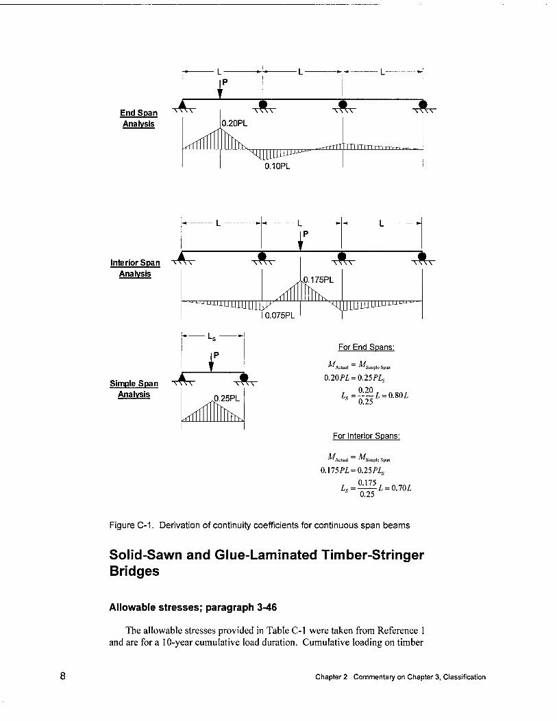
Ordinary continuous span bridges can be rated approximately using the concept of an "Equivalent Simple Span". The equivalent simple span is often thought of as the distance between live load inflection points on the continuous span bridge. In actuality, the equivalent span length is the length of a simple span that would receive the same maximum live load moment that would be produced on the continuous span by the same loading. The derivation of the recommended equivalent span lengths is demonstrated in Figure C-l. In actuality, these factors will vary for different load types (i.e. uniform load, single point load, or multiple point loads), different span length combinations, and different beam cross-sections along the length of the beam. The original TM5- 312 and FM5-446 (References 8 and 9) attempted to address these variations by providing equivalent span lengths for several different loading and span length combinations. However, all of these factors were within 14 percent of those for the one case shown in Figure C-l. Therefore, the all-encompassing factors of 0.80 times the length of the end span and 0.70 times the length of the interior span were chosen for sake of simplicity and expediency. These values are conservative and well within the required accuracy of these analytical procedures.


End Span Analysis

■^7 L

L-

TTvr 0.20PL

0.10PL

\T\\

■^-i-rrrnTTTITrrn-rrrrT-T^

\^\\

Interior Spa Analysis

n T^V

I

0.075PL

A Yr£175PL

\*\\

^[iUllliuu^XIJJJ

Simple Span Analysis

^w I

■YTW

0.25PL

For End Spans:

''"Actual = ^Simple Span

0.20PL = 0.25PL

I« = 0.20 0.25

Z. = 0.80£

For Interior Spans:

™ Actual _ "^Simple Span

0.175/'/, = 0.25 PL, ai75A = 070i

s 0.25

Figure C-1. Derivation of continuity coefficients for continuous span beams

Solid-Sawn and Glue-Laminated Timber-Stringer Bridges

Allowable stresses; paragraph 3-46

The allowable stresses provided in Table C-1 were taken from Reference 1 and are for a 10-year cumulative load duration. Cumulative loading on timber


refers to the total time that it is loaded to its maximum stress state (i.e. the time that a vehicle is on the bridge). Therefore, traffic volume, as opposed to the age of the structure, is a better indicator of cumulative loading. For relatively low volume military loadings on short-life (TO) bridges, the cumulative loading will be considerably lower than 10 years, which reflects every-day civilian cumulative loadings on permanent bridges (Stresses for every-day civilian loadings on permanent bridges are referred to in Reference 1 as "Inventory" allowable stresses). To account for the lower traffic volume, the allowable stresses in Table C-l may usually be increased by a factor of 1.33. This factor comes from Reference 2 and reflects the "Operating" level of rating, which is allowed for the occasional overloads that must cross civilian bridges. In general, the Operating rating is more applicable to the shorter-life, lower traffic volume TO bridges discussed in this manual.

Whenever the species and grade of solid-sawn timber cannot be determined, assume the allowable bending stress, F^, to be 1.75 ksi and the allowable

horizontal shear stress, Fv, to be 0.095 ksi. These values were originally

recommended in Reference 9. The Inventory allowable stresses recommended in Reference 1 are almost all greater than or equal to 1.3 ksi and 0.070 ksi for bending and shear, respectively, and therefore represent a conservative lower bound for timber stresses. Multiplying these values by the 1.33 factor to reflect the Operating level of service for TO bridges (see discussion above) gives approximately the recommended values of 7.75 and 0.095 ksi. Therefore, these values are reasonable and conservative and have been adopted for use in this manual. Note that these values must still be adjusted for the variable conditions listed in the footnotes of Table C-l.

The minimum values from Reference 1 for glued-laminated timber are 2.00 ksi and 0.155 ksi for F^ and Fv, respectively. Applying the 1.33 Operating level

multiplier as discussed above gives the values recommended herein of 2.66 ksi and 0.200 ksi for Fj, and Fv, respectively in glued-laminated beams where the

species and grade are unknown.

Applied dead load shear per stringer; paragraph 3-52

Reference 1, article 13.6.5.2 states that for uniformly distributed loads, such as dead load, the magnitude of vertical shear used in allowable load calculations should be the maximum shear occurring at a distance from the support equal to the bending member depth, d. Therefore, since shear from a uniform load decreases linearly from maximum at the support to 0 at midspan, the dead load shear, vpi at a distance, d, from the support will be:

(C-7) ii-d)

VDL ~ L

2

sup = v ' sup r id\

and

v _ <°DLL f sup ~ (C-8)


where,

vDL - dead load shear per stringer at distance, d, from support.

L = stringer span length. d = stringer depth. coD[ = applied dead load per foot of stringer (Equation 3-1).

Combining terms from Equations C-7 and C-8 and converting to allow for d in units of inches, yields Equation 3-7 for dead load shear per stringer:

v _a>DLL

V 6Zy (3-7)

Total live-load shear for one or two lanes; paragraph 3-54

The original versions of this manual (References 8 and 9) had a different version of the live load shear equation from that shown in Equation 3-9. Reference 11 found that this equation to be conservative in most cases, but recommended replacing it with the similar and more accurate equation from Reference 1. This recommendation was adopted herein. Article 13.6.5.2 of Reference 1 states that the live load shear per stringer, vn , should be:

vLL = 05[(0.60^ ) + (DF- VLL)] (C-9)

where,

VLl = maximum vertical shear from a wheel line load at a distance of 3d or L/4from the support, whichever is smaller.

DF = the fraction of the total shear, Vn, carried by one stringer.

Values of DF are provided in Table 3.23.1 of Reference 1.

In order to use Equation C-9 in this manual, it was converted to reflect the method of analysis used in the manual as follows: The term, Vn , above can be

made to correspond to the live load shear values provided in FM Appendix B of this manual as follows: Divide Vn by 2 to account for the use of axle loads (i.e.

two wheel lines) in this manual instead of line (i.e. 1/2 of an axle) loads as used in Reference 1. Also, Vn in the equation above represents the shear at a

distance of 3d or L/4 from the support, whichever is smaller. The shear values in FM Appendix B of this manual represent the maximum shear at the support. Assuming simply-supported spans, and that the L/4 condition will be smaller most of the time (this will generally be true for short spans, which are common with timber bridges), the shear at this point on the span is 3/4 of the value at the support. Using these conversions, Equation C-9 becomes:

Vu.-^l(0.60VLL)+{DF.VLL)] (C-10)

10 Chapter 2 Commentary on Chapter 3, Classification

where,

V = applied vertical shear from FM Appendix B of this manual.

The distribution factor, DF, must also be converted to the number of effective stringers, N, as used in this manual. As previously discussed, this is done by taking the inverse of the DF to convert from a portion of load carried by one member to the total number of members contributing to carrying that load. This value is then multiplied by 2 to convert from a wheel line load to an axle load (as required for the procedures in this manual). This conversion is represented by Equation C-5. Using this conversion, the equation above becomes:

v^ = _3_

16 (0.60rJ + '™u>

JVi .2 )

(C-ll)

where,

N12 - number of effective stringers from Table 3-3.

The equation is now converted to terms of this manual. However, the equation above is a "design-oriented" equation in that it yields the live load shear per stringer, vn . For use as a "rating equation", the equation is solved for Vn, and

results in 3-9 as follows:

VLL=533VLL 0.6 + *u

(3-9)

Tracked vehicles on glue-laminated stringer bridges; paragraph 3-55

Equation 3-9 is applicable for both wheeled and tracked vehicles on solid- sawn timber bridges and for wheeled vehicles only on glued-laminated bridges. Reference 11 points out that the distribution of shear for tracked vehicles on glued-laminated stringers will be significantly different due to the much wider stringer spacings and longer spans associated with glued-laminated stringers and the relatively short uniform loadings produced by tracked vehicles. Due to this combination, much more of the shear load will be concentrated near the stringer support. Since a support is a "hard point", the deck will not deflect significantly and thus little load can be distributed transversely to other stringers. Therefore, it is conservative to assume that all of a single track line (i.e. one side of the tank load) is carried by a single stringer. Thus, Reference 11 recommends the applied shear load on a single stinger to be:

V, VLL=-

LL for one-way traffic, and (C-12)

"LL LL for two-way traffic (C-13)

Chapter 2 Commentary on Chapter 3, Classification 11

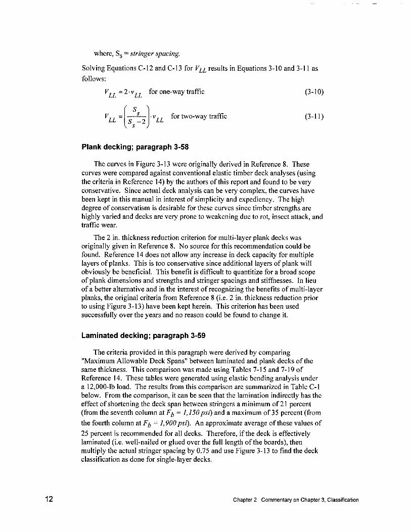
where, Ss = stringer spacing.

Solving Equations C-12 and C-13 for Vn results in Equations 3-10 and 3-11 as

follows:

Vj. = 2 • v.. for one-way traffic (3-10)

VLL

f S ^

S -2 v j . for two-way traffic (3-11)

Plank decking; paragraph 3-58

The curves in Figure 3-13 were originally derived in Reference 8. These curves were compared against conventional elastic timber deck analyses (using the criteria in Reference 14) by the authors of this report and found to be very conservative. Since actual deck analysis can be very complex, the curves have been kept in this manual in interest of simplicity and expediency. The high degree of conservatism is desirable for these curves since timber strengths are highly varied and decks are very prone to weakening due to rot, insect attack, and traffic wear.

The 2 in. thickness reduction criterion for multi-layer plank decks was originally given in Reference 8. No source for this recommendation could be found. Reference 14 does not allow any increase in deck capacity for multiple layers of planks. This is too conservative since additional layers of plank will obviously be beneficial. This benefit is difficult to quantitize for a broad scope of plank dimensions and strengths and stringer spacings and stiffnesses. In lieu of a better alternative and in the interest of recognizing the benefits of multi-layer planks, the original criteria from Reference 8 (i.e. 2 in. thickness reduction prior to using Figure 3-13) have been kept herein. This criterion has been used successfully over the years and no reason could be found to change it.

Laminated decking; paragraph 3-59

The criteria provided in this paragraph were derived by comparing "Maximum Allowable Deck Spans" between laminated and plank decks of the same thickness. This comparison was made using Tables 7-15 and 7-19 of Reference 14. These tables were generated using elastic bending analysis under a 12,000-lb load. The results from this comparison are summarized in Table C-l below. From the comparison, it can be seen that the lamination indirectly has the effect of shortening the deck span between stringers a minimum of 21 percent (from the seventh column at F^ = 1,150psi) and a maximum of 35 percent (from

the fourth column at Ff, = 1,900 psi). An approximate average of these values of

25 percent is recommended for all decks. Therefore, if the deck is effectively laminated (i.e. well-nailed or glued over the full length of the boards), then multiply the actual stringer spacing by 0.75 and use Figure 3-13 to find the deck classification as done for single-layer decks.


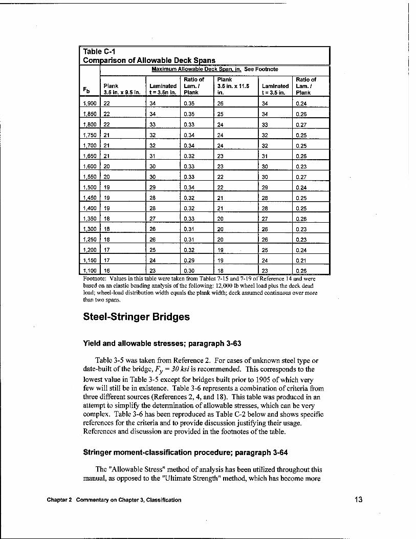
Table Com

(C-1 parison of Allowable Deck Spans

Fb

Maximum Allowable Deck Span. in. See Footnote

Plank 3.5 in. x 9.5 in.

Laminated t = 3.5n in.

Ratio of Lam./ Plank


Laminated t = 3.5 in.

Ratio of Lam./ Plank

1,900 22 34 0.35 26 34 0.24

1,850 22 34 0.35 25 34 0.26

1,800 22 33 0.33 24 33 0.27

1,750 21 32 0.34 24 32 0.25

1,700 21 32 0.34 24 32 0.25

1,650 21 31 0.32 23 31 0.26

1,600 20 30 0.33 23 30 0.23

1,550 20 30 0.33 22 30 0.27

1,500 19 29 0.34 22 29 0.24

1,450 19 28 0.32 21 28 0.25

1,400 19 28 0.32 21 28 0.25

1,350 18 27 0.33 20 27 0.26

1,300 18 26 0.31 20 26 0.23

1,250 18 26 0.31 20 26 0.23

1,200 17 25 0.32 19 25 0.24

1,150 17 24 0.29 19 24 0.21

1,100 16 23 0.30 18 23 0.26 Footnote: Values in this table were taken from Tables 7-15 and 7-19 of Reference 14 and were based on an elastic bending analysis of the following: 12,000 lb wheel load plus the deck dead load; wheel-load distribution width equals the plank width; deck assumed continuous over more than two spans.

Steel-Stringer Bridges

Yield and allowable stresses; paragraph 3-63

Table 3-5 was taken from Reference 2. For cases of unknown steel type or date-built of the bridge, Fy = 30 ksi is recommended. This corresponds to the lowest value in Table 3-5 except for bridges built prior to 1905 of which very few will still be in existence. Table 3-6 represents a combination of criteria from three different sources (References 2, 4, and 18). This table was produced in an attempt to simplify the determination of allowable stresses, which can be very complex. Table 3-6 has been reproduced as Table C-2 below and shows specific references for the criteria and to provide discussion justifying their usage. References and discussion are provided in the footnotes of the table.

Stringer moment-classification procedure; paragraph 3-64

The "Allowable Stress" method of analysis has been utilized throughout this manual, as opposed to the "Ultimate Strength" method, which has become more


widely accepted within the design community (Reference 1). The allowable stress method was utilized in this manual due to its simplicity and ease of understanding for the user.

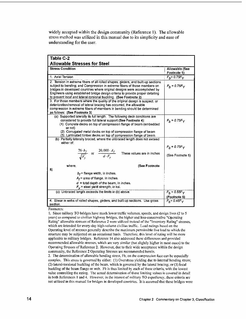
Table C-2 Allowable Stresses for Steel Stress Condition Allowable (See

Footnote 1) 1. Axial Tension Fb=0.75FY

2. Tension in extreme fibers of all rolled shapes, girders, and built-up sections subject to bending; and Compression in extreme fibers of those members on bridges in developed countries where original designs were accomplished by Engineers using established bridge design criteria to provide proper detailing to prevent local and lateral-torsional buckling. (See Footnote 2)

Fb = 0.75FY

3. Forthose members where the quality of the original design is suspect, or deterioration/removal of lateral bracing has occurred, the allowable compression in extreme fibers of members in bending should be determined as follows: (See Footnote 3)

(a) Supported laterally its full length. The following deck conditions are considered to provide full lateral support (See Footnote 4):

(1) Concrete decks on top of compression flange of beam (embedded or not)

(2) Corrugated metal decks on top of compression flange of beam (3) Laminated timber decks on top of compression flange of beam

Fb = 0.75Fy

(b) Partially laterally braced, where the unbraced length does not exceed either of:

16-bf 20,000-/l, —T=£- or — These values are in inches

where, (See Footnote 5)

bf= flange width, in inches.

Af= area of flange, in inches.

d = total depth of the beam, in inches. Fy= steel yield strength, in ksi.

Fb = 0.75FY

(See Footnote 5)

(c) Unbraced length exceeds the limits in (b) above. Fb = 0.55FY

(Footnote 6) 4. Shear in webs of rolled shapes, girders, and built-up sections. Use gross section.

Fb= OASFy

Footnotes: 1. Since military TO bridges have much lower traffic volumes, speeds, and design lives (2 to 5 years) as compared to civilian highway bridges, the higher and less-conservative "Operating Rating" allowable stresses of Reference 2 were utilized instead of the "Inventory Rating" stresses, which are intended for every-day high-volume civilian traffic. Load ratings based on the Operating level of stresses generally describe the maximum permissible live load to which the structure may be subjected on an occasional basis. Therefore, this level of rating will be more applicable to military bridges. Reference 14 also addressed these differences and provided recommended allowable stresses, which are very similar (but slightly higher in most cases) to the Operating Stresses of Reference 2. However, due to their wide acceptance within the design community, the Reference 2 Operating Stresses are recommended herein. 2. The determination of allowable bending stress, Fb, on the compression face can be especially complex. This stress is governed by either: (1) Overstress yielding due to internal bending stress; (2) lateral-torsional buckling of the beam, which is governed by the lateral bracing; or (3) local buckling of the beam flange or web. Fb is thus limited by each of these criteria, with the lowest value controlling the rating. The actual determination of these limiting values is covered in detail in both References 1 and 4. However, in the interest of military TO expediency, these criteria are not utilized in this manual for bridges in developed countries. It is assumed that these bridges were


designed and built using proper bracing details to insure that the beam can reach its full bending strength prior to any local or lateral-torsional buckling. 3. These criteria are intended for all bridges not covered by case 2 above. 4. Reference 2 only considers a beam "fully braced" when its top flange is embedded in the concrete deck. However, according to Reference 18, the other types of decks listed in this table also provide adequate lateral bracing. 5. These unbraced length equations come from Reference 18 and are used therein to represent the unbraced length below which the beam is still considered adequately braced to develop its full plastic moment. Therefore, these formulas should also represent unbraced length at which the upper limit (0.75Fy) of the complex allowable stress equation provided in Reference 2 (Table 6.6.2.1-2 for partially- or unbraced sections) can be reached. This equation was considered too complex for expedient military analyses. 6. For the case where the unbraced length exceeds the limits in part (c), the complex equation from Reference 2 should ideally be used for Fb. In order to avoid the use of this equation for expedient military classifications, the allowable stress for this condition was set at 0.55Fy, which is the upper limit of the equation at the Inventory Stress level. This value should be conservative in most cases since Reference 12 indicates that a beta value of 1.20 could be applied to this stress.

Composite-Stringer Bridges

Stringer section modulus; paragraph 3-72

Consider the stringer alone; i.e. only its section modulus and not that of the composite section. This is done to account for the assumption that the stringers were unsupported during construction of the bridge, thus making the stringers alone carry both their self-weight and that of the wet concrete. With this type of construction, the composite section is only considered to carry the live load, which is only applied after the concrete has cured and the section is composite.

Effective concrete- and steel-flange widths; paragraphs 3-73 and 3-74

The criteria given in paragraph 3-73 for effective concrete flange width came from Reference 1. For paragraph 3.74, Equivalent Steel Flange Width, the recommended values for fc' came from Article 6.6.2.4 of Reference 2.

Equation 3-12 for equivalent steel flange width was derived as follows:

At any given level of strain on a section, E, the corresponding level of stress, a, is:

(j = E-s (C-14)


where,

E = elastic modulus.

The total load, P, on the section with cross-sectional area, A, is thus:

P=a-A = E-e-A (C-15)

With this relationship, and assuming that at a given strain level, the total load, P, on the equivalent steel flange must equal to that on the actual concrete flange, the equivalent steel flange width, b', can be determined as follows:

P = P 1 steel ■* concrete ,„ 1 ,,

Es-e-As = Ec-s-Ac

where,

A = t-b, and t = flange thickness, and b = flange width.

Assuming the same steel flange thickness, t, as that of the concrete deck:

Es-t-b'=Ec-t-b" (C-17)

F h"

Es rm (3-12)

The values of rm came from Table 6.6.2.4 of Reference 2. Note that only the

"Operating" values are given from this table. This is done for the same reasons as discussed in footnote 1 of Table C-2 to account for the much lower level of traffic and design life associated with TO military bridges.

Steel-Girder Bridges

Effective number of girders for one- and two-lane traffic; paragraphs 3-83 and 3-84

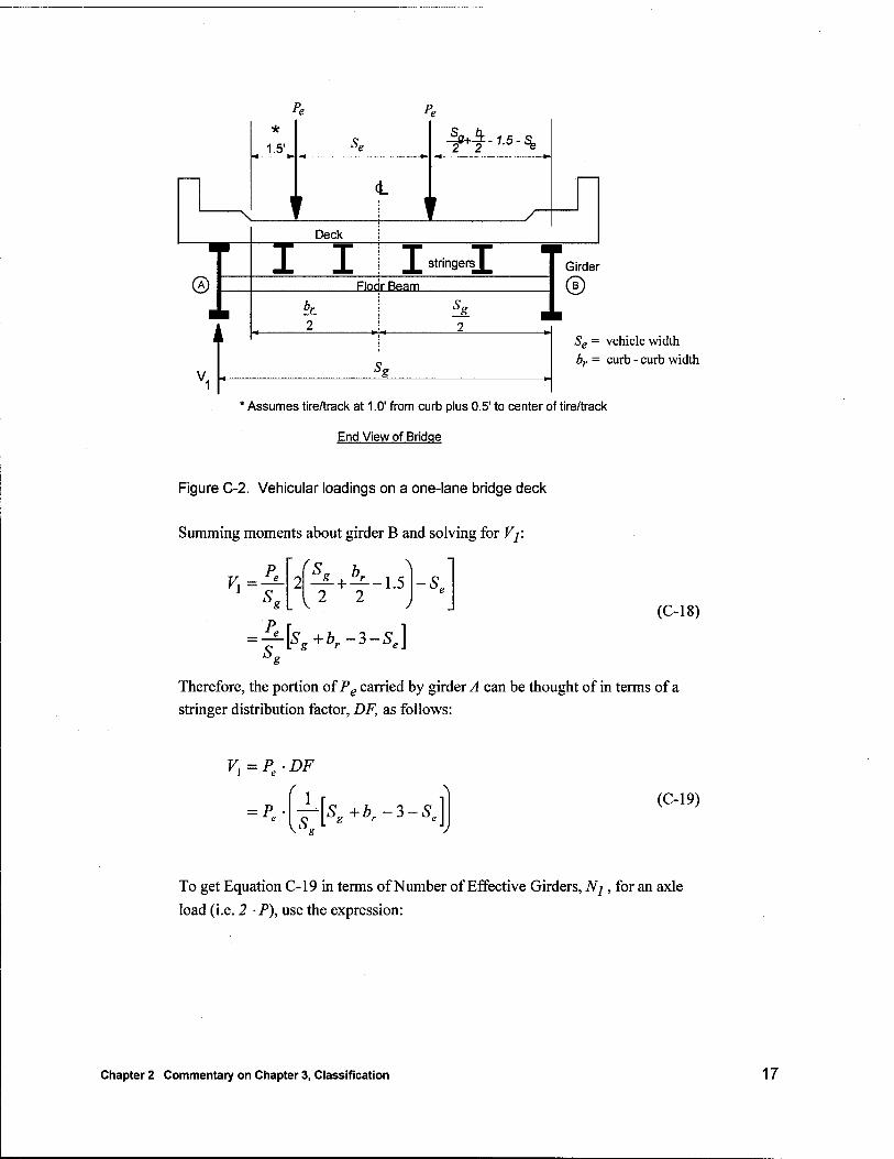
The effective number of girders may be derived by solving for the maximum reaction, V, that must be carried by a single girder from forces, Pe on the bridge

deck. Therefore, for one-way traffic, refer to Figure C-2 below for the definition of variables and solve for Fas follows:


Pe *

1.5'

Pe

Se , ¥^-1-5 •se

"

1 I V \ /

Deck !

I J_ X stringers | Girder (A) Floor Beam (!)

V

i 2

Sg 1

jSe = vehicle width

br = curb - curb width

* Assumes tire/track at 1.0' from curb plus 0.5' to center of tire/track

End View of Bridge

Figure C-2. Vehicular loadings on a one-lane bridge deck

Summing moments about girder B and solving for Vj:

P \ 2M- + ^-1.5

2 2 -S„

^8

(C-18)

Therefore, the portion of Pe carried by girder A can be thought of in terms of a stringer distribution factor, DF, as follows:

V,=Pe-DF

= P„ 1

KS, Sg+br-3-Se

(C-19)

To get Equation C-19 in terms of Number of Effective Girders, Nj , for an axle load (i.e. 2 -P), use the expression:


N, DF L[Sg+br-3-Se]

2Sg

Sg+br-3- (C-20)

The hypothetical military vehicles in FM Appendix B vary in width from 6 to 15 ft. Since this cannot be known before-hand in a load rating calculation, assume Se = 7 ft. This is a very conservative assumption in most cases since smaller

values of Se will produce larger values of Nj in Equation C-20. Equation 3-15

thus results as follows:

2Sg N =

1 S„+b -10 (3-15)

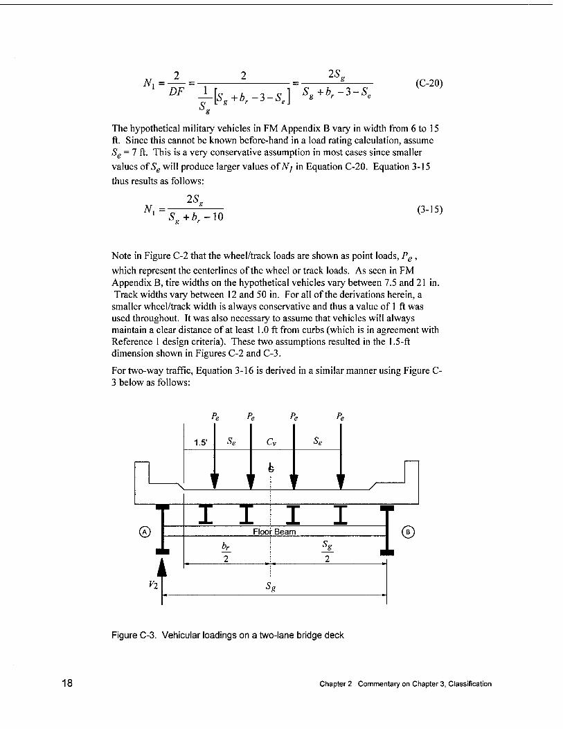
Note in Figure C-2 that the wheel/track loads are shown as point loads, Pe ,

which represent the centerlines of the wheel or track loads. As seen in FM Appendix B, tire widths on the hypothetical vehicles vary between 7.5 and 21 in. Track widths vary between 12 and 50 in. For all of the derivations herein, a smaller wheel/track width is always conservative and thus a value of 1 ft was used throughout. It was also necessary to assume that vehicles will always maintain a clear distance of at least 1.0 ft from curbs (which is in agreement with Reference 1 design criteria). These two assumptions resulted in the 1.5-ft dimension shown in Figures C-2 and C-3.

For two-way traffic, Equation 3-16 is derived in a similar manner using Figure C- 3 below as follows:

®|

Vl

Pe Pe

1.5' se Cv Se

k V V ! I ' 1

:r^ i i Floor Beam

2 2

s~

©

Figure C-3. Vehicular loadings on a two-lane bridge deck


V2 = Pe-DF=Pe

:.N2 =

A2r A

Sg+br-3.0-2Se-Q y*g

(C-21)

2 2 DF l-[Sg+br-3.0-2Se-

*g

-cj (C-22)

Sg+br-3.0-2Se-Cv

Assuming Se = 7 ft as discussed above:

•••y'-g.H-i7-c; <3-,6>

For normal two-lane bridges, *

Cv=br-2Se-3.0 > 2.0 feet (3-17)

For bridges with more than 2 lanes, this value will generally be far too conservative. For these special cases, the variable Cv should be determined by

the Engineer, based upon the actual curb-to-curb width, expected travel lanes for the convoys, the presence of median strips, convoy speed, and degree of traffic control. Note that Equation 3-17 indicates that the inside wheel line of the vehicle farthest away from the girder of interest will be located directly over the bridge centerline. This is a conservative assumption since convoys should normally drive in the center of their lanes. The minimum value of Equation 3-17 was set at 2.0 ft since adjacent vehicles will generally be at least 1 ft apart plus the distance to the center of the tires or tracks (which as discussed above have been assumed to be 1.0ft wide).

Stringer shear classification; paragraph 3-93

As previously discussed, shear is no longer considered for steel stringer bridges. However, because stringers in girder bridges are often relatively short, end shear may be a limiting factor and thus it must be checked. Stringer end shear may be limited by either the shear strength of the stringer web or by that of the connections to the floor beams. Since connections are generally designed to be stronger than the supported members (Article 10.19 of Reference 1), only web shear will be checked herein. In addition to this being a valid assumption, it is also a necessary assumption for TO bridges since bridge reconnaissance will generally be of too low resolution to obtain information on bolt or rivet details. Although not checked specifically, deteriorated connections should be accounted for by reducing the web shear rating by some appropriate amount to reflect the degree of deterioration of the connections; i.e. if the bolts appear to have lost x- percentage of their cross-section due to corrosion, the web cross-section used in the shear classification calculations should be reduced by the same percentage.


The distribution of shear to stringers depends significantly on the longitudinal, as well as the transverse, placement of loads on the bridge deck surface. The longitudinal placement of vehicles on the bridge which will maximize shear results in the vehicle being placed as close as possible to the reaction. The transverse distribution of these loads is then affected by the flexibility of the entire floor as well as the transverse placement of the loads. As the loads are moved longitudinally away from the reactions, the floor tends to deform more, resulting in distributions, which conform to those which are used for moment. Since the stringers do not deflect at the reactions, the loads are distributed laterally by the slab or deck behaving as if it were a series of simple beams supported by the stringers. This approach to shear distribution is the same as that used in Reference 1 and it requires case-by-case consideration of stringer spacing, stringer and deck type, and specific axle loadings and spacings for each rating vehicle. Variations of this approach, based on specific military vehicle configurations, were recommended in Reference 12 for design of military bridges. However, the design equations recommended in Reference 12 require known axle loadings for the "design" vehicle. This works well for design purposes where the design vehicle is specified initially or for a civilian load classification where only a few rating vehicles are used. However, it cannot be used for military load classification where 32 different rating vehicles (and thus axle configurations) are used and the specific one is unknown until the analysis is complete. Therefore, in lieu of an in-depth and costly study to determine a more accurate shear distribution equation, it has been conservatively assumed herein that the total shear from a single wheel or track "line" is carried by a single stringer. Converting to "axle" loading terms (as required in the FM Appendix C shear data) and applying the 15-percent impact factor, the total live-load shear, VLL, is thus:

2v,, V»'1E (3-30)

This equation would be far too conservative for the longer stringers associated with a "stringer bridge". However, it should work well for the relatively short stringers associated with girder bridges since in most cases the vehicle will be longer than the stringer span and thus only one axle can be on a stringer span at a time. The worst-case shear loading location for a single axle will be at the support where, as discussed above, very little transverse load distribution will occur. The equation should also work well for tracked vehicles since they provide a uniform loading over a relatively short length and thus little lateral distribution will occur. In addition, the equation above should also be applicable for two-way traffic since stringers on girder bridges will be generally be closely spaced, allowing only one wheel line per stringer. It is again reminded that the above equation should not be used for design purposes. The vehicle-specific design equations recommended in Reference 12 should be used for design.


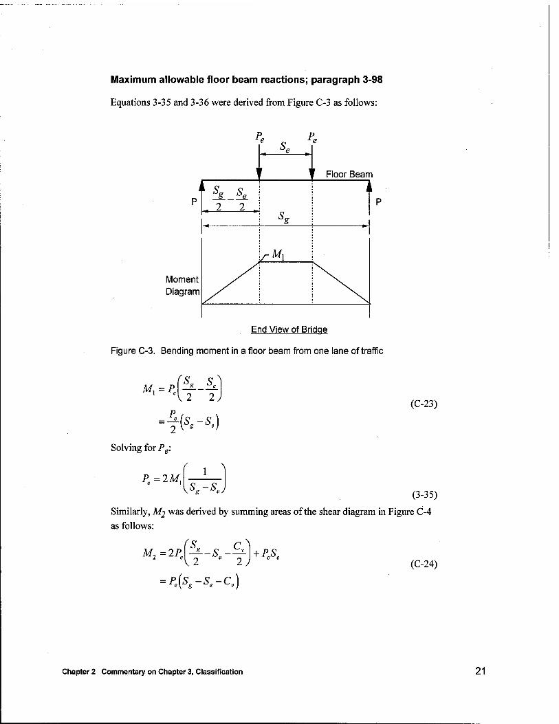
Maximum allowable floor beam reactions; paragraph 3-98

Equations 3-35 and 3-36 were derived from Figure C-3 as follows:

Pe Pe se

t t Floor Beam

1 Sz Se

.2 2 „ S

g

{

/-M\

Moment Diagram

End View of Bridge

Figure C-3. Bending moment in a floor beam from one lane of traffic

Solving for Pe:

P=2M, ' 1 ^

\Sg~Sey>

(C-23)

(3-35)

Similarly, M-2 was derived by summing areas of the shear diagram in Figure C-4

as follows:

M2=2Pe[^--Se-^\+PeSe

= pe(sg-se-cv) (C-24)


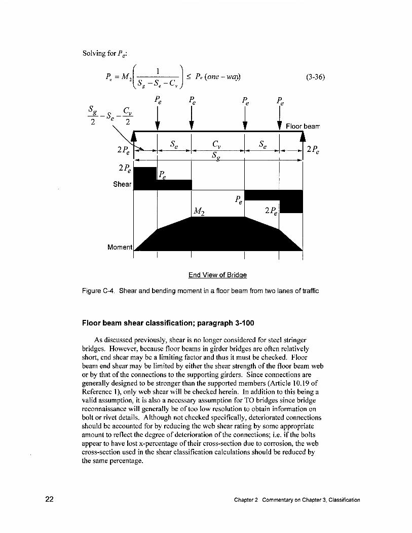
Solving for Pe

Pe=M2 ySg ~Se~Cv J

< Pe {one - waj) (3-36)

_JL_c _^Y_

P P Le re P P 1 e * e

LJ M Floor beam

2Pe

2Pe

Shear

I. se cv se i

: ' Sp

Pe

M2

Pe 2Pe

Moment

- 2/>

End View of Bridge

Figure C-4. Shear and bending moment in a floor beam from two lanes of traffic

Floor beam shear classification; paragraph 3-100

As discussed previously, shear is no longer considered for steel stringer bridges. However, because floor beams in girder bridges are often relatively short, end shear may be a limiting factor and thus it must be checked. Floor beam end shear may be limited by either the shear strength of the floor beam web or by that of the connections to the supporting girders. Since connections are generally designed to be stronger than the supported members (Article 10.19 of Reference 1), only web shear will be checked herein. In addition to this being a valid assumption, it is also a necessary assumption for TO bridges since bridge reconnaissance will generally be of too low resolution to obtain information on bolt or rivet details. Although not checked specifically, deteriorated connections should be accounted for by reducing the web shear rating by some appropriate amount to reflect the degree of deterioration of the connections; i.e. if the bolts appear to have lost x-percentage of their cross-section due to corrosion, the web cross-section used in the shear classification calculations should be reduced by the same percentage.


Maximum allowable floor beam reactions; paragraph 3-104

Equations C-19 and C-21 for maximum live load shear in floor beams were derived previously from Figures C-2 and C-3, and are repeated below as follows:

- For one-way traffic:

( V = P lmax e

1

vV Sg+br-3-Se > P

- For two-way traffic:

V-, = P ' 2max *■ e 2L.[Sg+br-3.0-2Se-Cv] > 2Pa

(C-19)

(C-21)

In order to use these equations for load class analysis, they must be solved for Pe

, which can then be used in the Floor Beam Pe curves in Figures 3-21 through 3- 24. Therefore:

- For one-way traffic:

Pe = VLLSg Sg+br-3.0-Se

> v LL

For two-way traffic

VT,S P.=

"LL"g

Sg+br-3.0-2Se-C > VLLy

(3-40)

(3-41)

Special allowance for caution crossing; paragraph 3-105

If a higher load rating for shear is required than that obtained from Equations 3-40 and 3-41, then a special "Caution Crossing" allowance may be calculated. However, in order to use these equations, the convoys must be carefully monitored on the bridge and must drive as close to the center of their respective lanes as possible. If control cannot be maintained, these equations should not be used. If the convoy is assumed to be perfectly centered on the bridge deck, the value of Pe can be derived from Figure C-5 as follows:


Pe Pe JeJ Pe ' P e r e c ^

V \ v v v 1 V v , i I A A i i

One-Wav Traffic Two-Way Traffic

Figure C-5. Shear effects from vehicles centered in their lanes

-For one-way traffic:

Vr- = Pe

or

Pe = VU.

For two-way traffic:

v2 = 2Pe

or

Pe2 1

(3-42)

(3-43)

These equations will provide the highest possible rating for floor beam shear. They may be used in place of Equations 3-40 and 3-41 if desired for a careful caution crossing where vehicles will stay near the center of their respective lanes (transversely).

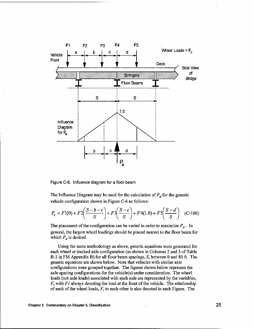
Maximum floor beam reactions; figures 3-21 through 3-24

The hypothetical vehicles and corresponding bending moment and shear data in FM Appendix B are unchanged from the preceeding manuals (References 8 and 9). These data are governed by STANAG 2021 and cannot be changed. The new curves in Figures 3-21 through 3-24 were derived by the authors to provide a better and more accurate means for assessing loading effects on transverse floor beams. Their derivation is summarized as follows:

Assume that stringers are simply-supported between floor beams. Therefore, only the wheel/track loads on stringers immediately adjacent to (i.e. connected to) the floor beam of interest will contribute to the floor beam reaction. Therefore, the loading for maximum floor beam reaction, Pe, can be represented

by the "Influence Diagram" shown in Figure C-6 below:


F1 F2 F3 F4 F5 Wheel Loads = F„

\fehicle |* Front

I Floor Beams T

Side View of

Bridge

b eil d ■« »-^—•> ■* ■>

R

Figure C-6. Influence diagram for a floor beam

The Influence Diagram may be used for the calculation of Pe for the generic

vehicle configuration shown in Figure C-6 as follows:

Pe=Fl(0) + F2 S-b-c

+ F3 S-c

+ F4(\.0) + F5 S-d

(C-100)

The placement of the configuration can be varied in order to maximize Pe. In

general, the largest wheel loadings should be placed nearest to the floor beam for which Pe is desired.

Using the same methodology as above, generic equations were generated for each wheel or tracked axle configuration (as shown in Columns 2 and 3 of Table B-l in FM Appendix B) for all floor beam spacings, S, between 0 and 80 ft. The generic equations are shown below. Note that vehicles with similar axle configurations were grouped together. The figures shown below represent the axle spacing configurations for the vehicle(s) under consideration. The wheel loads (not axle loads) associated with each axle are represented by the variables, F, with Fl always denoting the load at the front of the vehicle. The relationship of each of the wheel loads, F, to each other is also denoted in each Figure. The


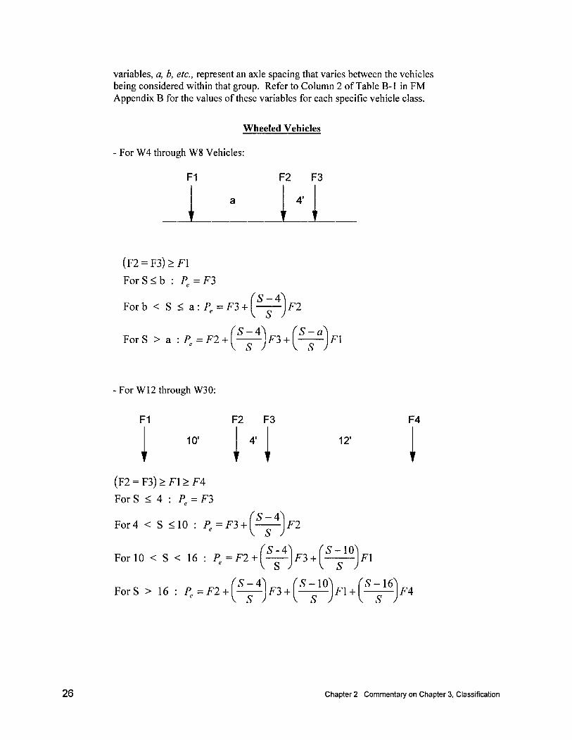
variables, a, b, etc., represent an axle spacing that varies between the vehicles being considered within that group. Refer to Column 2 of Table B-l in FM Appendix B for the values of these variables for each specific vehicle class.

Wheeled Vehicles

- For W4 through W8 Vehicles:

F1 F2 F3

4'

(F2 = F3) > F\

For S < b : Pe = F3

Forb < S < &:P=F3 + \——\F2

'S-4\ (S-a\ ForS > a : P. = F2 + —— F3+ —— \Fl

- For W12 through W30:

F1

10"

F2 F3

4'

(F2 = F3) > F\ > FA

For S < 4 : Pe = F3

(S-f For4 < S <10 : P=F3 + \ \F2

12'

For 10 < S < 16 : P'=F2 + S-4

s ; F3 + S-10^

ForS > 16 : P'=F2 + 'S-4\ , s ) F3 +

5-10

s )

F1 +

F4

F\

S-\6 FA


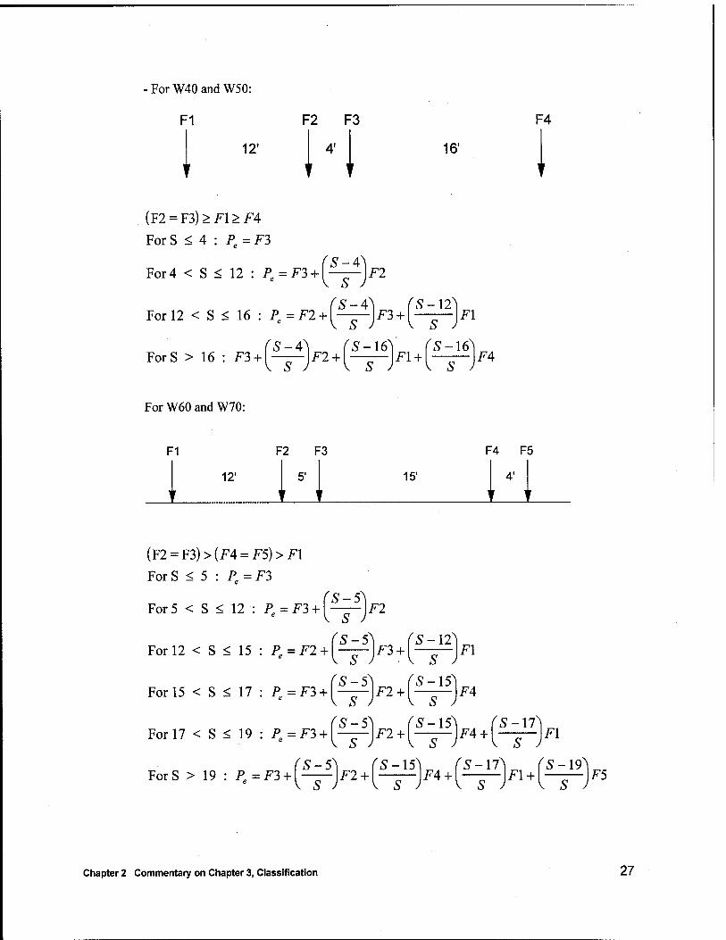
-ForW40andW50:

F1 F2 F3 F4

12' 4' 16'

♦ I ♦ t

(F2 = F3) > F\ > FA

For S < 4 : Pe = F3

[S-4] For 4 < S < 12 : Pe = F3 + \ ——

V S ) F2

(S-4\ For 12 < S < 16 : Pe = F2 +1 ——-J F3

(S-\2) + { S J Fl

(S-4) ForS > 16 : F3+ ——

V 5 J F1 +

(S-l6] I s )F4

ForW60andW70:

F1 F2 F3 F4 F5

12' 5' 15' 4' v u v M V

(F2 = F3)>(F4 = F5)>F1

For S < 5 : Pe = F3

(S-5] For 5 < S < 12 : Pe = F3 +1 ——-J F2

For 12 < S < 15 : Pe = F2 + [—J F3 + [—^-^ Fl

For 15 < S < 17 : P.=F3 + \^)F2 + \-^-\F4

For 17 < S < 19 : P'= F3 +1 —— IF2 +

K S

S-15 F4 + [-j-\Fl

ForS > 19 : P'=F3 + S-5

V S F2 + \-

(S-15)^A fS-17^1 (S -19 V S

F4+ ■ V S J

F\ + \- V 5

F5


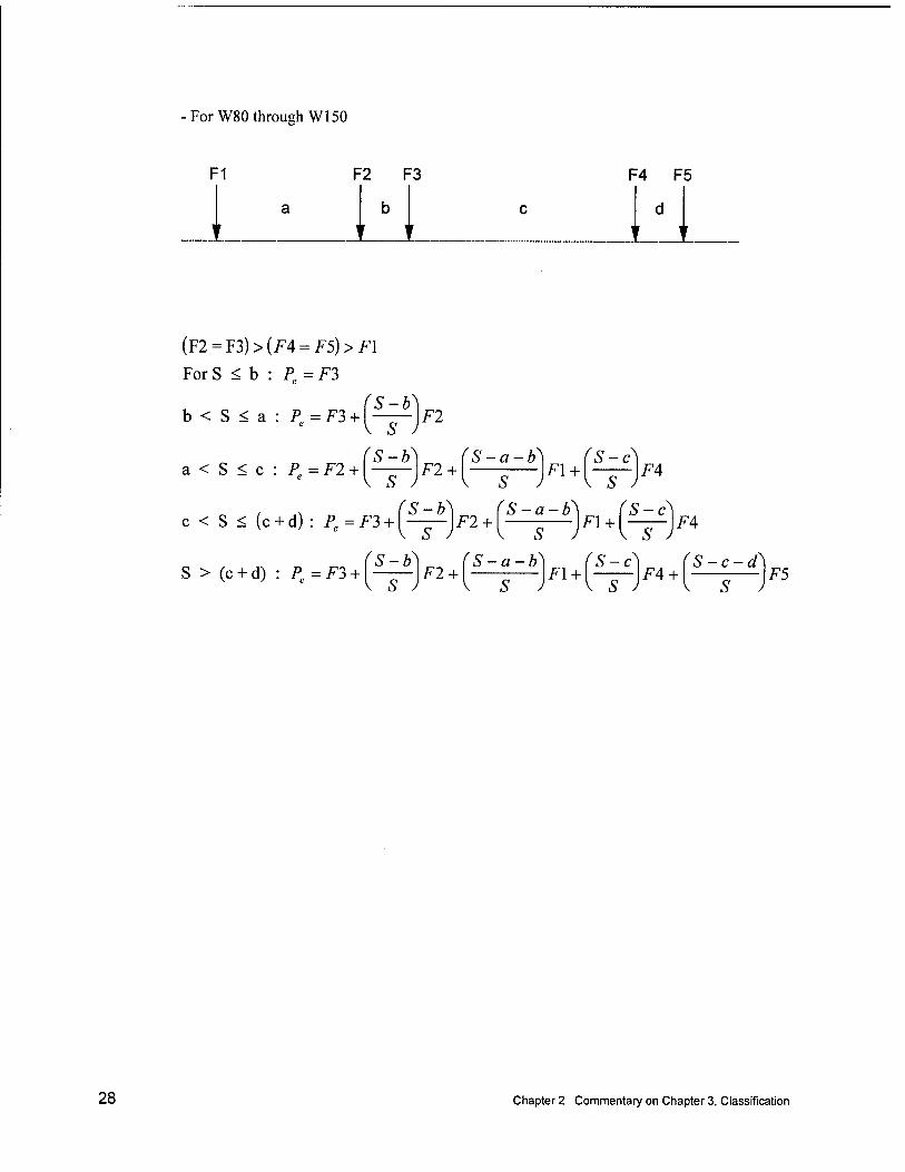
- For W80 through Wl 50

F1 F2 F3

b

F4 F5

d

(F2 = F3)>(F4 = F5)>F1

For S < b : P'= F3

b<S<a:P=F3 +

a<S<c:P=F2 +

S-b) s )

S-b

F2

F2 + S-a-b

Fl + Is) FA

c < S < (c + d) : P = F3 + {■ (S-b'

\ S J F2 +

S-a-b

V S J Fl +

S-c

S J FA

S > (c + d) : Pe = F3 + I S J

F2 + S-a-b

F\ + S-c

F4 + S-c-d

\ S F5


Tracked Vehicles

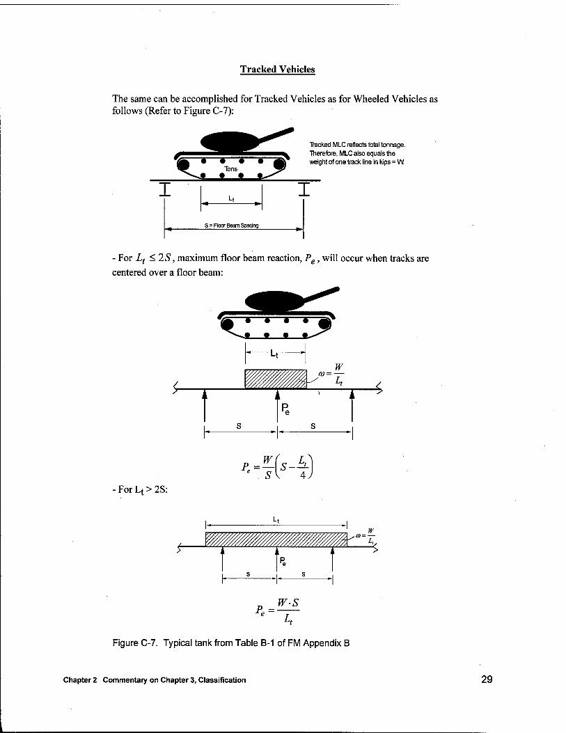
The same can be accomplished for Tracked Vehicles as for Wheeled Vehicles as follows (Refer to Figure C-7):

'<m * * * • •? W Tons y

Tracked MLC reflects total tonnage. Therefore, MLC also equals the weight of one track line in kips = W

- For Lt <2S, maximum floor beam reaction, Pe, will occur when tracks are centered over a floor beam:

•^ * * • • AT

Lt

W

/ W////////////// «=—

• "*

—±—-

i

Pe

—-5 ►

, '

ForLt>2S:

p.A*-k) e . S\ 4J

M w ■

' '/////V/ > 1 I

s

i i

Pe

S

i >

Pe = w-s

Figure C-7. Typical tank from Table B-1 of FM Appendix B


Truss Bridges

Expedient classification; paragraph 3-113

Trusses are generally of a balanced design, where all structural members are designed to carry the same live loadings. Therefore, it is reasonable to assume that the floor system was designed for the same live loads as the main truss members and that both will thus have the same MLC.

Total dead load; paragraph 3-115

Equations 3-44 and 3-45 for total dead load of a truss bridge are from the original Reference 8. No earlier reference could be found for these equations. However, due to their ease of use, as compared to actual dead load calculations, it was highly desirable to keep them in this manual. Other "shortcut" equations like these are very commonly used in bridge design, where the dead load must be estimated before the members are actually sized (Reference 16). They are used for a "first-cut" at the dead loads to be expected. In order to validate these equations, they were tested against specific trusses with carefully-calculated dead loads (Reference 5). These test cases indicate that the equations work quite well and tend to always err on the conservative side.

Compressive force in top chord; paragraph 3-120

The allowable stress of a concentrically loaded, thin, column-type member, such as the top chord of a truss, will usually be limited by its buckling capacity, which is a function of the KL/r ratio. Table 3-9 comes directly from Reference 2.

Reinforced Concrete Slab Bridges

Assumptions; paragraph 3-131

The analytical methodology described below is only applicable to slab bridges with the main reinforcing running parallel to the direction of traffic. The slab acts as a one-way slab in the direction of traffic. Assume that the area above the neutral axis acts in compression and that the reinforcing steel in the bottom of the slab carries all of the tension (i.e. assume the concrete carries no tension). The assumed stress distribution, using the Whitney Equivalent Rectangular Stress Block, is shown in Figure 3-34. Only the moment capacity is determined for the slab since shear generally will not control in thin reinforced concrete members. Only a 1-ft wide strip of slab at the midspan should be considered. While all of the previous analysis methods have used the Allowable Stress method of analysis, the Ultimate Strength (sometimes called Load Factor) method is used for all of the following reinforced concrete analyses. This method has been used


for many years by concrete analysts and is thus the most familiar. This is also the same method that was used in the two previous manuals (References 8 and 9).

Concrete and reinforcing steel strengths; paragraphs 3-132 and 3-133

Table 3-10 provides suggested values for concrete compressive strength, fc', when it is unknown. Likewise, Table 3-11 provides suggested steel yield strength, Fy, when it cannot be obtained from other sources. Both of these tables

come directly from Reference 2.

Compressive stress block depth; paragraph 3-135

Equation 3-60 comes from Reference 1 and was modified for this manual as follows:

A.tFv A.tFv

0.85(l2m)/c 10.2/c

where,

12 in. represents the assumed 1-ft width of slab, for which all calculations are made.

Slab moment capacity; paragraph 3-136

Equation 3-61 comes from Reference 1 and was modified as follows:

m = 0.9 ft \

12/n/ A*Fy 2) = 0.07 5 AstFy

( d0\

. 2) (3-61)

Allowable live load moment; paragraph 3-138

Equation 3-63 represents the amount of bending moment that is available to carry live load. It is determined by subtracting the moment required to carry the dead load, mDL , from the total available moment capacity, m. It is then divided by the impact factor of 1.15. This equation is basically the same as Equation 3-4. The only difference in this equation is that the dead load and live load moments are multiplied by a safety factor (sometimes called "load factors") of 1.3 as required for the Ultimate Strength method. The value of 1.3 was chosen based upon the recommendations of Reference 2 for an "Operating" level of traffic. This term describes a higher allowable loading for occasional loads that are not expected on a day-to-day basis throughout the life of the bridge. This describes military loads, as compared to civilian loads, because they are of much lower frequency and military bridge life requirements are much shorter. Equation 3-63 is thus derived from Reference 2 as:


m-l.3mn, m-\3mnr mLL = < \ = — 0-63) LL (1.3)1.15 1.5

where 1.15 is impact factor and 1.3 is the safety factor.

For emergency conditions where a lower factor of safety may be mandated, the live load safety factor may be set equal to 1.0 since military loadings should be fairly well known. The equation will then become:

m - \3mn, m„ = — (3-64) u 1.15 V '

Effective slab width; paragraph 3-139

Equation 3-65 comes from Reference 1 and is multiplied by 2 to account for axle loads (used in the FM analyses) instead of wheel lines (used in AASHTO analyses). Note that it does not distinguish between one- and two-way traffic. For slabs, this is only limited by lane width restrictions.

Reinforced Concrete T-Beam Bridges

Assumptions; paragraph 3-143

As with all other bridge types, and in accordance with Reference 2, the interior beams are assumed to control the classification. The exterior beams are assumed to have equal or greater capacity than the interior beams. As with the slab bridge, the T-beam bridge is analyzed only on the basis of moment capacity (i.e. shear will generally not control the rating). The deck is also assumed to have sufficient thickness that it will not control the rating, and is thus not rated.

Moment capacity; paragraphs 3-145 through 3-148

All of the criteria and equations used to calculate moment capacity came directly from Reference 1. Equations 3-70 and 3-74 were divided by 12 to get in terms of feet instead of inches.

Prestressed Concrete Bridges

Analytical classification; paragraph 163

Military bridges are rated on the basis of ultimate capacity, with little concern for serviceability criteria such as cracking and deflection. All of the procedure herein is basically in accordance with Reference 1 for flexural strength of beams.


Moment capacity; paragraphs 3-164 through 3-174

Concrete and steel strength criteria in paragraph 3-164 are from Reference 2. Effective Flange Width criteria in paragraph 3-165 represent a conservative and simplified combination of the criteria from Reference 1. In paragraph 3-166, effective flange width, b", is used in Equations 3-81 and 3-82 since positive moment at midspan is assumed to control. For this scenario, b = b". The average stress in prestressing steel, Equation 3-84 comes directly from Reference 1, with

* Y

a value of — = 0.5 used. A

All moment capacity equations in paragraph 3-172 come from Reference 1. A value of <j) = 0.9 was used throughout. The equations were also divided by 12 to convert from inch-kips to foot-kips. The safety factors in Equations 3-96 and 3-97 are the same as those for the slab and T-beam bridges (previously discussed).

Arch Bridges

Modern arch bridge; paragraph 3-179

An exact analysis procedure for arch bridges is very tedious and time- consuming. Procedures for exact arch analysis require that the loading conditions be known; the very item that is being sought in military bridge classification procedures. Additionally, many arches are structurally indeterminate, greatly increasing the analytical difficulty. Fortunately, arches are generally of a balanced design, where all structural members are designed to carry the same live loadings. Therefore, it is reasonable to assume that the floor system was designed for the same live loads as the main arch structural members and that both will thus have the same MLC. Additionally, the main arch members of long-span bridges are also designed for many secondary forces such as wind, uneven deflection, etc., making them considerably stronger than the floor system if only live load is considered. Therefore, it is more conservative to only consider the floor system for live load considerations.

Masonry arch bridge; paragraphs 3-180 through 3-183

Masonry arch design/analysis is a very old "art" and most existing procedures are empirical, based on years of experience. The empirical procedure presented herein was originally provided in Reference 8 and its origin prior to that could not be found. It has since been used with success by such authors as Reference 7.


3 Commentary on Chapter 6, Design of Bridge Superstructures

Deck Design

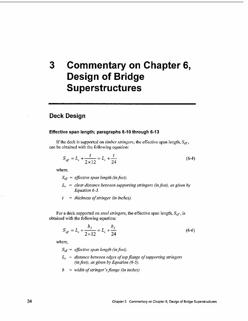
Effective span length; paragraphs 6-10 through 6-13

If the deck is supported on timber stringers, the effective span length, Scjf, can be obtained with the following equation:

Scfr =Lc+—— = LC+— (6"4) eff c 2x12 c 24

where,

Sejf = effective span length (in feet).

Lc = clear distance between supporting stringers (in feet), as given by Equation 6-3.

t = thickness of stringer (in inches).

For a deck supported on steel stringers, the effective span length, Scg, is obtained with the following equation:

Seff =LC+ —+— = 4 + — (6-6) eff c 2x12 24

where,

Seff = effective span length (in feet).

Le = distance between edges of top flange of supporting stringers (in feet), as given by Equation (6-5).

b = width of stringer's flange (in inches)

34 Chapter 3 Commentary on Chapter 6, Design of Bridge Superstructures

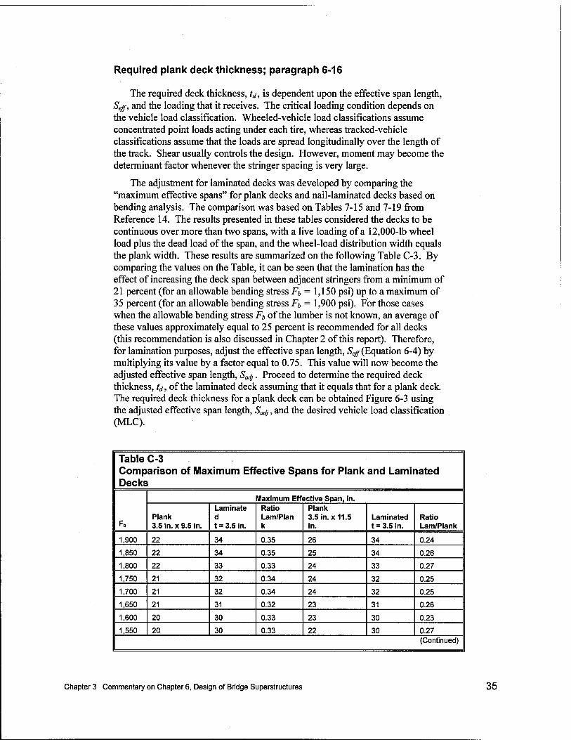
Required plank deck thickness; paragraph 6-16

The required deck thickness, td, is dependent upon the effective span length, Seff, and the loading that it receives. The critical loading condition depends on the vehicle load classification. Wheeled-vehicle load classifications assume concentrated point loads acting under each tire, whereas tracked-vehicle classifications assume that the loads are spread longitudinally over the length of the track. Shear usually controls the design. However, moment may become the determinant factor whenever the stringer spacing is very large.

The adjustment for laminated decks was developed by comparing the "maximum effective spans" for plank decks and nail-laminated decks based on bending analysis. The comparison was based on Tables 7-15 and 7-19 from Reference 14. The results presented in these tables considered the decks to be continuous over more than two spans, with a live loading of a 12,000-lb wheel load plus the dead load of the span, and the wheel-load distribution width equals the plank width. These results are summarized on the following Table C-3. By comparing the values on the Table, it can be seen that the lamination has the effect of increasing the deck span between adjacent stringers from a minimum of 21 percent (for an allowable bending stress F* = 1,150 psi) up to a maximum of 35 percent (for an allowable bending stress Fb = 1,900 psi). For those cases when the allowable bending stress Ft of the lumber is not known, an average of these values approximately equal to 25 percent is recommended for all decks (this recommendation is also discussed in Chapter 2 of this report). Therefore, for lamination purposes, adjust the effective span length, Seg- (Equation 6-4) by multiplying its value by a factor equal to 0.75. This value will now become the adjusted effective span length, SadJ. Proceed to determine the required deck thickness, td, of the laminated deck assuming that it equals that for a plank deck The required deck thickness for a plank deck can be obtained Figure 6-3 using the adjusted effective span length, Sadj, and the desired vehicle load classification (MLC).

Table C-3 Comparison of Maximum Effective Spans for Plank and Laminated Decks

Fb

Maximum Effective Span, in.


Laminate d t = 3.5 in.

Ratio Lam/Plan k


Laminated t = 3.5in.

Ratio Lam/Plank

1,900 22 34 0.35 26 34 0.24

1,850 22 34 0.35 25 34 0.26

1,800 22 33 0.33 24 33 0.27

1,750 21 32 0.34 24 32 0.25

1,700 21 32 0.34 24 32 0.25

1,650 21 31 0.32 23 31 0.26

1,600 20 30 0.33 23 30 0.23

1,550 20 30 0.33 22 30 0.27 (Continued)

Chapter 3 Commentary on Chapter 6, Design of Bridge Superstructures 35

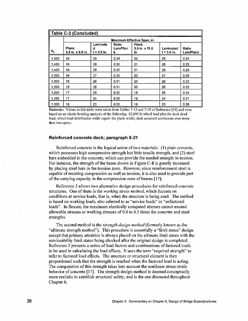
Table C-3 (Concluded)

Fb

Maximum Effective Span, in.


Laminate d t=3.5in.

Ratio Lam/Plan k


Laminated t=3.5in.

Ratio Lam/Plank

1,500 19 29 0.34 22 29 0.24

1,450 19 28 0.32 21 28 0.25

1,400 19 28 0.32 21 28 0.25

1,350 18 27 0.33 20 27 0.26

1,300 18 26 0.31 20 26 0.23

1,250 18 26 0.31 20 26 0.23

1,200 17 25 0.32 19 25 0.24

1,150 17 24 0.29 19 24 0.21

1,100 16 23 0.30 18 23 0.26

Footnote: Values in this table were taken from Tables 7-15 and 7-19 of Reference [14] and were based on an elastic bending analysis of the following: 12,000 lb wheel load plus the deck dead load; wheel-load distribution width equals the plank width; deck assumed continuous over more than two spans.

Reinforced concrete deck; paragraph 6-21

Reinforced concrete is the logical union of two materials: (1) plain concrete, which possesses high compressive strength but little tensile strength, and (2) steel bars embedded in the concrete, which can provide the needed strength in tension. For instance, the strength of the beam shown in Figure C-8 is greatly increased by placing steel bars in the tension zone. However, since reinforcement steel is capable of resisting compression as well as tension, it is also used to provide part of the carrying capacity in the compression zone of beams [17].

Reference 3 allows two alternative design procedures for reinforced-concrete structures. One of them is the working stress method, which focuses on conditions at service loads, that is, when the structure is being used. The method is based on working loads, also referred to as "service loads" or "unfactored loads". In flexure, the maximum elastically computed stresses cannot exceed allowable stresses or working stresses of 0.4 to 0.5 times the concrete and steel strengths.

The second method is the strength design method (formerly known as the "ultimate strength method"). This procedure is essentially a "limit states" design except that primary attention is always placed on the ultimate limit states with the serviceability limit states being checked after the original design is completed. Reference 3 presents a series of load factors and combinations of factored loads to be used in calculating the load effects. It uses the term "required strength" to refer to factored load effects. The structure or structural element is then proportioned such that the strength is reached when the factored load is acting. The computation of this strength takes into account the nonlinear stress-strain behavior of concrete [17]. The strength design method is deemed conceptually more realistic to establish structural safety, and is the one discussed throughout Chapter 6.


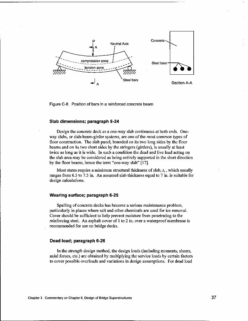
p 4A

Neutral Axis

compression zone

tension zone

J 777777' Steel bars

Concrete

Steel bars

Section A-A

Figure C-8. Position of bars in a reinforced concrete beam

Slab dimensions; paragraph 6-24

Design the concrete deck as a one-way slab continuous at both ends. One- way slabs, or slab-beam-girder systems, are one of the most common types of floor construction. The slab panel, bounded on its two long sides by the floor beams and on its two short sides by the stringers (girders), is usually at least twice as long as it is wide. In such a condition the dead and live load acting on the slab area may be considered as being entirely supported in the short direction by the floor beams, hence the term "one-way slab" [17].

Most states require a minimum structural thickness of slab, ts, which usually ranges from 6.5 to 7.5 in. An assumed slab thickness equal to 7 in. is suitable for design calculations.

Wearing surface; paragraph 6-25

Spalling of concrete decks has become a serious maintenance problem, particularly in places where salt and other chemicals are used for ice removal. Cover should be sufficient to help prevent moisture from penetrating to the reinforcing steel. An asphalt cover of 1 to 2 in. over a waterproof membrane is recommended for use on bridge decks.

Dead load; paragraph 6-26

In the strength design method, the design loads (including moments, shears, axial forces, etc.) are obtained by multiplying the service loads by certain factors to cover possible overloads and variations in design assumptions. For dead load


computations, this factor equals 1.4. The dead load of slab can be found upon substitution into the following equation:

wDL=\A t. U, x

12 1,000 + 1.4 x

12 1,000 = 1.4

12,000 (6-7)

where,

wDL = dead load of slab (in kips/ft/ft of width).

ts = slab thickness (in inches).

Uc = unit weight for concrete (in lb/ft3), as given in Table 6-4.

tw = wearing surface thickness (in inches).

Uw = unit weight for wearing surface material (in lb/ft3), as given in

Table 6-4.

Live load; paragraph 6-28

The maximum-single axle load for a hypothetical MLC vehicle is given by Column Number 4 in Table B-l of FM Appendix B. The critical concentrated live load per wheel used for design is given as,

2 kips IU on 1 u

3-wheels/axle,, = P„ (6-9)

where,

1 LL

ÜL~ =

critical concentrated live load per wheel (in kips).

maximum single-axle load (in tons), as obtained from Column

Number 4 of Table B-l in FM Appendix B.

For slabs continuous over three or more supports, a continuity factor of 0.8 shall be applied. Also, an allowance for dynamic, vibratory, and impact effects should be applied in the design of concrete slabs. For military bridges, the factor to account for impact effects will be equal to 1.15, and the live load factor is equal to 1.7. Therefore, the live load moment will be determined as,

MLL = 1.7 x 0.8 x 1.15 32 J

Pu. = 1-564 Seff+2-\

y 32 J ■ LL (6-10)

where,

MLL = live load bending moment of slab (in kips-ft/ft of width).

Pu = critical concentrated live load per axle (in kips), as given by

Equation (6-9). Seff = effective span length (in feet), as given by Equation (6-4).


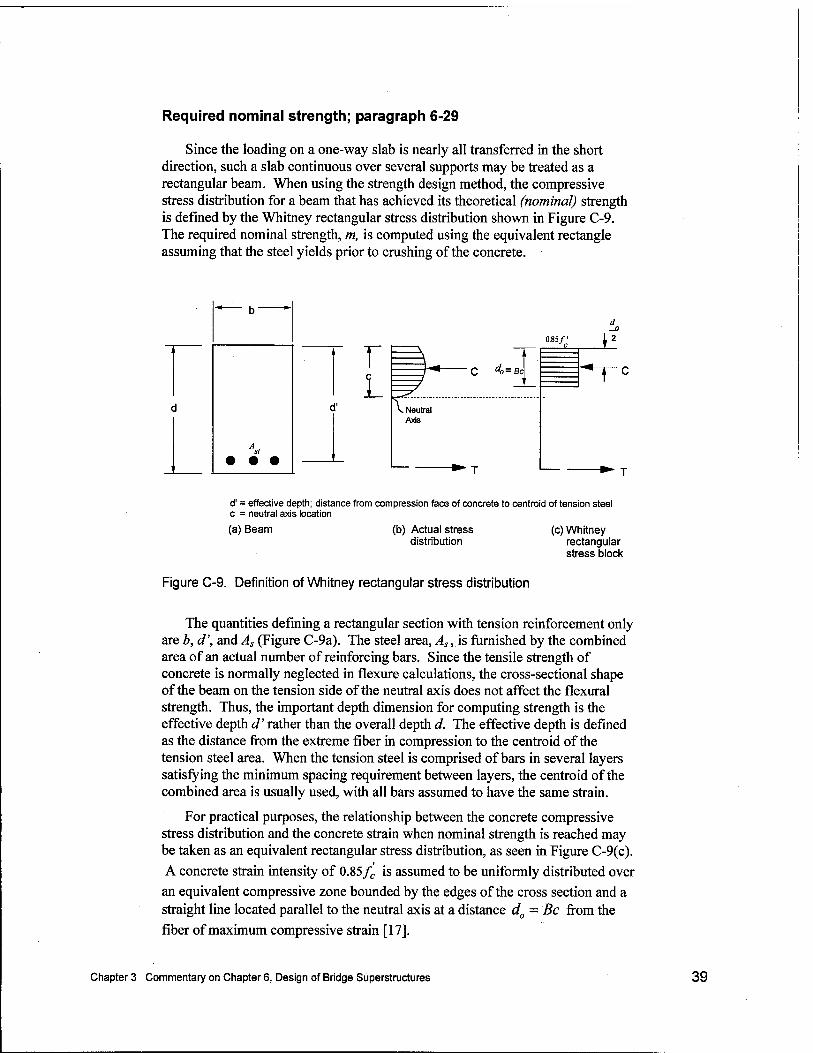
Required nominal strength; paragraph 6-29

Since the loading on a one-way slab is nearly all transferred in the short direction, such a slab continuous over several supports may be treated as a rectangular beam. When using the strength design method, the compressive stress distribution for a beam that has achieved its theoretical (nominal) strength is defined by the Whitney rectangular stress distribution shown in Figure C-9. The required nominal strength, m, is computed using the equivalent rectangle assuming that the steel yields prior to crushing of the concrete.

r r L

d'

0.85/' c

d

\2

\ ^ -1 -^—,—

) ^ (: "o - üc J t

\ Neutral Axis

d' = effective depth; distance from compression face of concrete to centroid of tension steel c = neutral axis location

(a) Beam (b) Actual stress distribution

(c) Whitney rectangular stress block

Figure C-9. Definition of Whitney rectangular stress distribution

The quantities defining a rectangular section with tension reinforcement only are b, d', and As (Figure C-9a). The steel area, As, is furnished by the combined area of an actual number of reinforcing bars. Since the tensile strength of concrete is normally neglected in flexure calculations, the cross-sectional shape of the beam on the tension side of the neutral axis does not affect the flexural strength. Thus, the important depth dimension for computing strength is the effective depth d' rather than the overall depth d. The effective depth is defined as the distance from the extreme fiber in compression to the centroid of the tension steel area. When the tension steel is comprised of bars in several layers satisfying the minimum spacing requirement between layers, the centroid of the combined area is usually used, with all bars assumed to have the same strain.

For practical purposes, the relationship between the concrete compressive stress distribution and the concrete strain when nominal strength is reached may be taken as an equivalent rectangular stress distribution, as seen in Figure C-9(c).

A concrete strain intensity of 0.85/<! is assumed to be uniformly distributed over

an equivalent compressive zone bounded by the edges of the cross section and a straight line located parallel to the neutral axis at a distance d0 = Be from the

fiber of maximum compressive strain [17].


The factored load moment, Mu, for a section in bending is obtained by

applying load factors (i.e. overload provision) to the moments due to dead load and live load. Then, the required nominal strength, m, of a section can be calculated by dividing the factored moment, Mu, by a strength reduction factor

<j> = 0.9 that accounts for adverse variations in material strengths, workmanship,

dimensions, control, and degree of supervision, even though all are within accepted tolerances. The strength requirement for flexure is acceptable if it

satisfies that the design strength m > m.

Reinforcing steel ratio; paragraph 6-30

The reinforcement ratio, Rs, may be conveniently used to represent the

relative amount of tension reinforcement in a beam. In order to have reasonable assurance for a ductile mode of failure in flexure, Reference 3 limits the amount of tension steel to a value greater than the minimum reinforcement ratio, min Rs,

that is,

min Rs = (C-22) Jy

where,

min Rs = minimum reinforcement ratio Rs .

f = yield strength of reinforcing steel (in psi).

but equal to or less than 75 percent of the amount in the balanced strain condition, that is,

max Rs = 0.75 Rbs (C-23)

where,

max Rs = maximum reinforcement ratio Rs .

RbK = reinforcement ratio in the balanced strain condition, as given by Equation C-24.

Thus, the reinforcement ratio in the balanced strain condition, Rbs, is given as,

J V

r 87,000 ^

v87,000 + /y/

(C-24)


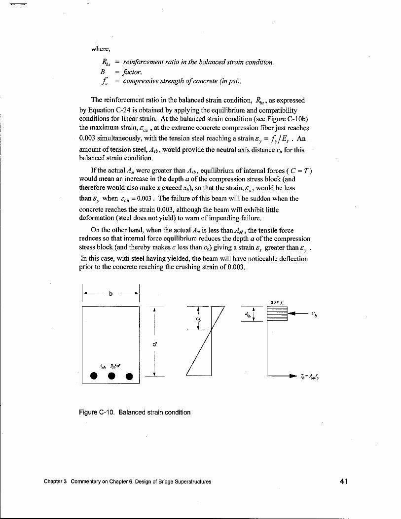
where,

i?fa = reinforcement ratio in the balanced strain condition. B = factor. f'c = compressive strength of concrete (in psi).

The reinforcement ratio in the balanced strain condition, Rbs, as expressed

by Equation C-24 is obtained by applying the equilibrium and compatibility conditions for linear strain. At the balanced strain condition (see Figure C-lOb) the maximum strain, s^ , at the extreme concrete compression fiber just reaches

0.003 simultaneously, with the tension steel reaching a strain s = fy/Es . An

amount of tension steel, Asb, would provide the neutral axis distance cb for this balanced strain condition.

If the actual Ast were greater than Asb, equilibrium of internal forces (C = T) would mean an increase in the depth a of the compression stress block (and therefore would also make x exceed xb), so that the strain, ss, would be less

than s when scu = 0.003 . The failure of this beam will be sudden when the

concrete reaches the strain 0.003, although the beam will exhibit little deformation (steel does not yield) to warn of impending failure.

On the other hand, when the actual Ast is less than Asb, the tensile force reduces so that internal force equilibrium reduces the depth a of the compression stress block (and thereby makes c less than cb) giving a strain ss greater than s .

In this case, with steel having yielded, the beam will have noticeable deflection prior to the concrete reaching the crushing strain of 0.003.

0.85 /;

Tb = Asbfy

Figure C-10. Balanced strain condition


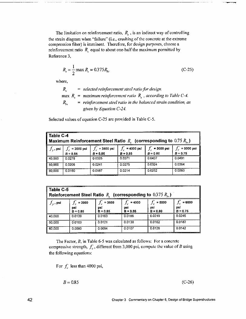
The limitation on reinforcement ratio, Rs , is an indirect way of controlling

the strain diagram when "failure" (i.e., crushing of the concrete at the extreme compression fiber) is imminent. Therefore, for design purposes, choose a reinforcement ratio Rs equal to about one-half the maximum permitted by

Reference 3,

R. 1

maxi? = 0375Ä ts (C-25)

where,

Rs = selected reinforcement steel ratio for design.

max Rs = maximum reinforcement ratio Rs , according to Table C-4.

Rbs = reinforcement steel ratio in the balanced strain condition, as

given by Equation C-24.

Selected values of equation C-25 are provided in Table C-5.

Table C-4 Maximum Reinforcement Steel Ratio Rs (corresponding to 0.75 Rbs)

fy.PS* f'c = 3000 psi

B = 0.85

f'c = 3500 psi

B = 0.85

fc = 4000 psi

B = 0.85

f'c = 5000 psi

B = 0.80

f'c - 6000 psi

8 = 0.75

40,000 0.0278 0.0325 0.0371 0.0437 0.0491

50,000 0.0206 0.0241 0.0275 0.0324 0.0364

60,000 0.0160 0.0187 0.0214 0.0252 0.0283

Table C-5 Reinforcement Steel Ratio Rs (corresponding to 0.375 Rhs)

fyPS'1 /c=3000

psi B = 0.85

fc ■ 3500

psi B = 0.85

/c' =4000

psi B = 0.85

/c'=5000

psi B = 0.80

/; =6000

psi B = 0.75

40,000 0.0139 0.0163 0.0186 0.0219 0.0246

50,000 0.0103 0.0121 0.0138 0.0162 0.0182

60,000 0.0080 0.0094 0.0107 0.0126 0.0142

The Factor, B, in Table 6-5 was calculated as follows: For a concrete compressive strength, f'c, different from 3,000 psi, compute the value of B using

the following equations:

For fc less than 4000 psi,

B = 0.85 (C-26)


For f'c greater than 4000 psi,

'/;-4000 5 = 0.85-0.05

V 1000 > 0.65 (C-27)

where,

B = factor. f'c = compressive strength of concrete (in psi), as obtained from Table 6-2.

Strength coefficient of resistance; paragraph 6-31

In the design of rectangular sections in bending with tension reinforcement only, the problem is to determine b, d\ and As from the required value of the required nominal strength m = (MDL + MLL )/0.9, and the given material

properties f'c and fy.

Assuming that the steel has already yielded when the concrete strength is reached, the internal forces can be obtained. The compressive force C is the summation of the compressive stresses acting on the compression concrete area, and is given as:

C = 0.S5f;bdo (C-28)

where,

C = compressive force (in kips). f'c = compressive strength of concrete (in psi). b = beam cross-section width (in inches). d0 = depth of compressive stress block (in inches), as seen in

Figure C-lOc.

For the ductile failure condition, the tensile force T is

T=Astfy (C-29)

where,

T = tensile force (in kips). Ast = area of tension steel (in square inches).

fy = yield strength of reinforcing steel (in psi).


The area of steel can be conveniently represented using the dimensions shown in Figure C-10a as,

Asl=Rsbd' (C-30)

where,

Ast - area of tension steel (in square inches).

Rs = selected reinforcement ratio for design.

b = beam cross-section width (in inches). d' = effective depth, that is, the distance from compression face of

concrete to centroid of tension steel (in inches).

According to Figure C-9(c), the two conditions of equilibrium are,

C = T

and

(C-31)

r d \ m'= (C orT) d' 0

V n (C-32)

where m' is the design nominal strength of the section. Using the preset reinforcement ratio R , it follows that:

/ R,

/v \

Substituting Equation C-33 into Equation C-32, the design strength is given as

J y

(C-33)

m'=Rsbd'f 2 0.85/;

d' (C-34)

A strength coefficient of resistance Rn is obtained by dividing Equation C-34 by

bd'2 so that,

R =- m'

bd' = RS /, ( R f 4 S J 1

s J y 1- s J y

1.7/e

(

-K A s J y

c J

(Rs Y(fy )

1.7/c" (6-12)

Effective depth; paragraph 6-32

The required effective depth d' is the distance from the compression face of concrete to the centroid of tension steel, as depicted in Figure C-9 (a). This distance can be determined using the following equation,

required bd' m

(C-35)


which can be rewritten as,

,, m x 12,000 m x 1,000 reqd'=J = (C-36)

where,

req d' = required effective depth (in inches).

m = required nominal strength (in kips-fi), as given by Equation 6-11.

Rn = strength coefficient of resistance (inpsi), as given by Equation 6-12.

b = beam cross-section width (in inches), in this case equal to 12 in. since the design is for a 12-in.-wide (1-ft-wide) strip.

Assume a No. 6 steel bar (db = 0.75 in.) plus an additional 3/4 in. (for protective concrete cover). Assuming also that the bars will fit in one layer, the required overall depth is calculated as,

0.75 reqh = reqd' + —— + 0.75 = reqd' + 1.125 (C-37)

where,

req h = required overall depth (in inches),

req d' = required effective depth (in inches), as given by Equation (6-14).

Increase the required overall depth obtained by Equation C-14 by approximately 0.5 in. (or by an amount that will round the required overall depth to the next complete inch or half-inch, whichever is closest). This will become the final thickness ts of the concrete deck. Now compute the effective depth d' as follows,

0.75 d' = (reqh + 0.5) - —— - 0.75 = reqh - 0.625 (C-38)

where,

d' = effective depth (in inches). req h = required overall depth (in inches), as given by Equation (6-13).

By combining Equations (6-37) and (C-38), it simplifies into the equation for obtaining the effective depth of slab,

Im x I 000 d'=reqd' + 1.125 - 0.625 = -1 + 0.5 (6-14)


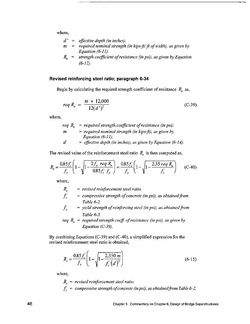
where,

d' m

K =

effective depth (in inches). required nominal strength (in kips-fi/ft of width), as given by Equation (6-11). strength coefficient of resistance (in psi), as given by Equation

(6-12).

Revised reinforcing steel ratio; paragraph 6-34

Begin by calculating the required strength coefficient of resistance Rn as.

m x 12,000 reqRn =

<\2 \2(d') (C-39)

where,

req Rn = required strength coefficient of resistance (in psi).

m = required nominal strength (in kips-ft), as given by Equation (6-11).

d = effective depth (in inches), as given by Equation (6-14).

The revised value of the reinforcement steel ratio Rs is then computed as,

R = 0.85/;

where.

fc

1-1- 2fy reqR„

0.85/; fy j

0.85/;

fy 1-Jl-

2.35 req R,,

fc (C-40)

= revised reinforcement steel ratio.

= compressive strength of concrete (in psi), as obtained from

Table 6-2. f = yield strength of reinforcing steel (in psi), as obtained from

Table 6-3. req Rn = required strength coeff of resistance (in psi), as given by

Equation (C-39).

By combining Equations (C-39) and (C-40), a simplified expression for the revised reinforcement steel ratio is obtained,

R = 0.85/'

fy 1- 1-

2,350 m

m (6-15)

where,

Rs = revised reinforcement steel ratio.

f'c = compressive strength of concrete (in psi), as obtained from Table 6-2.


fy = yield strength ofreinforcing steel (in psi), as obtained from Table 6-3.

m = required nominal strength (in kips-fi), as given by Equation (6-11). d = effective depth (in inches), as given by Equation (6-14).

Bar selection and placement; paragraph 6-35

Compute the actual spacing between bars as,

12 - (2 x 0.75) - (no. of bars x d,) Bar Spacing ■■

total no. of bars -1 (C-41)

10.5 -(no. of bars xd,) '

total no. of bars — 1

where,

Bar Spacing = actual spacing between bars (in inches). no. of bars = number ofreinforcing bars selected from Table 6-6

that will accommodate the total area of steel computed in Equation (6-16).

db = nominal diameter of the bar (in inches), as obtained from Table 6-6.

total no. of bars = total number of bars to be accommodated within the beam's width.

Stringer Design

Live load moment; paragraph 6-51

The sudden application of live loads, such as vehicles driving, breaking, accelerating, and bouncing on the bridge is referred to as impact loads. The effects of impact loading must be taken into account by increasing the live loads by 15 percent. This factor should be used for all stringer-bridge types and span lengths, and has already been taken into consideration when computing the amount of live load moment that each stringer must resist in Equation (6-24).

Each structural component of a bridge helps to distribute the applied live loads in various ways. This load sharing is taken into consideration by applying an effective number of stringers, N!i2, which depend on the number of traffic lanes. These values can be obtained using Table 3-3 in Chapter 3 according to deck type and using the actual stringer spacing.

Allowable stresses; paragraphs 6-53 through 6-55

Structural elements are designed so that unit stresses computed under the action of service loads do not exceed predesignated allowable values. Since


military TO bridges have significantly lower traffic volume when compared to civilian highway bridges, higher and less conservative allowable stress values can be used for practical purposes. These stress values correspond to "Operating" conditions rather than to "Inventory" conditions. An operating level of stresses describes the maximum permissible live load to which a structure may be subjected on an occasional basis. On the other hand, an inventory level of stresses is intended for everyday high-volume civilian traffic. Therefore, the operating level of stress results more applicable for military bridges conditions.

The allowable stresses for timber provided in FM Appendix C correspond to a 10-year cumulative load duration. Cumulative loading on a timber member refers to the total time that the specimen is loaded to its maximum stress state (i.e. the time that a vehicle load remains on the bridge). Therefore, traffic volume is a good indicator of cumulative loading. For relatively low volume of military loading on short-life TO bridges, the cumulative loading will be considerably lower than 10 years. This compares to an everyday civilian cumulative loading on a permanent bridge. To account for the lower traffic volume, the allowable stresses in FM Appendix E should be increased by a factor equal to 1.33. This factor reflects an operating level of stress, which is included for the occasional overloads that may experience a civilian bridge.

Operating level allowable stresses were used for steel for the same reasons as discussed above. The steel yield strengths listed in Table 6-7 came from Reference 1.

Vertical deflection check; paragraph 6-58

After the beams are selected, they should be checked for span vertical deflection. The vertical deflection of the stringers due to live load plus impact is limited to 1/200 of the span length. If the deflection exceeds this limitation, damage to the deck and curb system may occur.

The maximum deflection, dmax, for a simply supported beam subjected to a concentrated load is given by,

"MAX ~ PL'

48£/ = dLL

and the maximum moment is computed as,

MMAX _PL _

4 -MLL

(C-42)

(C-43)

The above equation can be rewritten as,

L


The maximum moment acting on a single beam is the total moment of the span distributed among the total number of stringers, as follows:

M MAX M LL

*v Nv (C-45)

The moment of inertia can be expressed in terms of the section modulus and the depth of the stringer as follows,

s-L (C-46)

and knowing that

d c = —

2 (C-47)

we can obtain the following expression for the moment of inertia of the beam,

I = S£. (C-48)

Finally the expression for the live load deflection including impact can be written as,

( 1.15

dix=-

4M \

LL

KNvLJ (\12% in3A

4USd " lft3 (C-49)

V 2

which upon simplification yields,

_33WLLL2

ULL ~

NxaESds

(6-27)

dLL = deflection due to live load plus impact (in inches).

M'LL = total design live load moment according to vehicle class (in kips-ft).

L = design span length (in feet). Ni,2 = effective number of stringers, as given by Table 3-3. E = modulus of elasticity (in ksi), see FM Appendix Cfor timber or

FMAppendix Dfor steel. S = section modulus of the selected stringer (in ksi), see FM Appendix C

for timber or FM Appendix Dfor steel. ds = depth of the stringer (in inches).


Maximum allowable unbraced length; paragraph 6-64

Establish the maximum allowable unbraced length, Lc , for a steel stringer as

the smaller of the values obtained from the following equations,

76 bf 1 6.33 bf L =—r^-x — = —r=£ (C-25a) • ^ n 4K

20,000 1 1.667

(</,/4)F, 12 (rf,M)F,

where,

Lc = maximum allowable unbraced length for a steel stringer (in feet).

bf = flange width of the steel section (in inches), as obtained from

FMAppendix F. F = yield strength of steel (in ksi), as obtained from Table 6-9.

ds = depth of the steel section (in inches), as obtained from

FM Appendix F. As = area of steel section (in square inches), as obtained from

FM Appendix F.

Design live load shear per stringer; paragraph 6-85

Tests have indicated that shear failure will occur when a concentrated load is at some constant distance from the bridge support. Shear failure does not occur when the load is just off the support (where the maximum shear is produced). When a concentrated load is just off the support, it tends to compress the support's fibers, thus increasing the horizontal shear strength. The optimum condition for shear failure exists when the load moves off the support a distance equal to three times the stringer depth, but not more than one-fourth the span length. Therefore, the effective live load shear per stringer should be reduced accordingly to obtain the design live load shear per stringer, but its value must always be greater than or equal to 0.75 vUj.


References

1. American Association of State Highway and Transportation Officials. (1992). "Standard specifications for highway bridges," 15th ed., Washington, DC.

2. American Association of State Highway and Transportation Officials. (1994). "Manual for condition evaluation of bridges". Washington, DC.

3. American Concrete Institute. (1983). "Building code requirements for reinforced concrete (ACI318-83)," Detroit, MI.

4. American Institute of Steel Construction. (1980). Manual of steel construction, 8th ed., Chicago, IL.

5. Fu, C. C. (Unpublished). "Report of selected test cases for the truss formula in FM5-446," Military Fixed Bridges. Unpublished Report from the University of Maryland, College Park, MD.

6. Gaylord, E.H., and Gaylord, C. N. (1990). Structural Engineering Handbook. Chapter 18, 3rd ed., McGraw Hill, New York.

7. Harvey, W. J. and Smith, F. W. (1995). British Practice in Arch Bridge Assessment. Proceedings from Fourth International Bridge Engineering Conference, United Kingdom.

8. Headquarters, Department of the Army. (1968). "Military Fixed Bridges," Technical Manual TM5-312, Washington, DC.

9. Headquarters, Department of the Army. (1991). "Military Nonstandard Fixed Bridges," Field Manual FM5-446, Washington, DC.

10. Heins, C. P., and Firmage, D. A. (1979). Design of Modern Steel Highway Bridges, John Wiley & Sons, Chapter 3, New York, NY.

11. Knab, L. I., Moody, R .C, Sanders, W. W. Jr., Elleby, H. A. (1977). "Design criteria for theater of operations glued-laminated timber highway bridges," Vol 1, and 2, Construction Engineer Research Laboratory, Technical Report M-198, Champaign, IL.

12. Knab, L. I., Moody, R .C, Sanders, W. W. Jr., Elleby, H. A. (1977). "Design criteria for theater of operations glued-laminated steel highway bridges," Vol 1, and 2;Construction Engineer Research Laboratory, Technical Report M-195, Champaign, IL.

13. MacGregor, J. G. (1992). Reinforced Concrete: Mechanics and Design. Chapter 2, 2nd ed., Prentice Hall, New Jersey.

References 51

14. Ritter, Michael A. (1992). "Timber bridges: design, construction, inspection, and maintenance," EM 7700-8. U.S. Department of Agriculture, Forest Service.

15. Roberts, N. P. (1959). "Load distribution effects in bridge deck systems," Unpublished Report.

16. Texas Department of Transportation, Division of Bridges and Structures. (1993). "Texas bridge load rating program," Users Manual, Austin, Tx.

17. Wang, C, and Salmon, C. G. (1985). Reinforced Concrete Design, Harper Row, 4th ed., New York, NY.

18. Yura, J.A. Phillips, B., Raju, S., and Webb, S. (1993). "Bracing effects of bridge decks," Report No. 1239-4F, Center for Transportation Research, University of Texas, Austin, TX.

52 References

REPORT DOCUMENTATION PAGE Form Approved OMB No. 0704-0188

Public reporting burden for this collection of information is estimated to average 1 hour per response, including the time for reviewing instructions, searching existing data sources, gathering and maintaining the data needed, and completing and reviewing this collection of information. Send comments regarding this burden estimate or any other aspect of this collection of information, including suggestions for reducing this burden to Department of Defense, Washington Headquarters Services, Directorate for Information Operations and Reports (0704-0188), 1215 Jefferson Davis Highway, Suite 1204, Arlington, VA 22202-4302. Respondents should be aware that notwithstanding any other provision of law, no person shall be subject to any penalty for failing to comply with a collection of information if it does not display a currently valid OMB control number PLEASE DO NOT RETURN YOUR FORM TO THE ABOVE ADDRESS.

1. REPORT DATE (DD-MM-YYYY) August 2002

2. REPORT TYPE Final report

3. DATES COVERED (From - To)

4. TITLE AND SUBTITLE 5a. CONTRACT NUMBER

Technical Commentary on FM3-34.343, "Military Nonstandard Fixed Bridging" 5b. GRANT NUMBER

5c. PROGRAM ELEMENT NUMBER

6. AUTHOR(S)

James C. Ray, Yazmin Seda-Sanabria

5d. PROJECT NUMBER

5e. TASK NUMBER

5f. WORK UNIT NUMBER

7. PERFORMING ORGANIZATION NAME(S) AND ADDRESS(ES)

U.S. Army Engineer Research and Development Center Geotechnical and Structures Laboratory 3909 Halls Ferry Road Vicksburg,MS 39180-6199

8. PERFORMING ORGANIZATION REPORT NUMBER

ERDC/GSLTR-02-15

9. SPONSORING / MONITORING AGENCY NAME(S) AND ADDRESS(ES)

U.S. Army Corps of Engineers Washington, DC 20314-1000

10. SPONSOR/MONITOR'S ACRONYM(S)

11. SPONSOR/MONITOR'S REPORT NUMBER'S!

12. DISTRIBUTION / AVAILABILITY STATEMENT

Approved for public release; distribution is unlimited. 13. SUPPLEMENTARY NOTES

14. ABSTRACT

This report provides a supplementary commentary to the newly revised Army field manual, FM 3-34.343, "Military Nonstandard Fixed Bridging," which was published by Headquarters, Department of the Army, on 12 February 2002. Past editions of Technical and Field Manuals for the military have had no documentation or references by which the content could be verified or checked. In an effort to alleviate this problem, the U.S. Army Engineer Research and Development Center (ERDC) has prepared this commentary on Chapter 3, "Classification," and Chapter 6, "Design of Bridge Superstructures," which were the only chapters written by the ERDC. This report provides a detailed explanation/derivation of all simplified methodologies and equations within those chapters.

15. SUBJECT TERMS Bridge assessment FM3-34.343

Military nonstandard fixed bridging

16. SECURITY CLASSIFICATION OF:

a. REPORT

UNCLASSIFIED

b. ABSTRACT

UNCLASSIFIED

c. THIS PAGE

UNCLASSIFIED

17. LIMITATION OF ABSTRACT

18. NUMBER OF PAGES

60

19a. NAME OF RESPONSIBLE PERSON James C. Ray

19b. TELEPHONE NUMBER (include area code)

(601)634-3839 Standard Form 298 (Rev. 8-98) Prescribed by ANSI Std. 239.18

Documents

Technical Commentary on FM3-34.343, Military Nonstandard