Technical Challenges of Exascale Computing

JASONThe MITRE Corporation

7515 Colshire DriveMcLean, Virginia 22102-7508

(703) 983-6997

Contact: Dan McMorrow — dmcmorrow@mitre.org

JSR-12-310

April 2013

Approved for public release; distribution unlimited.

Contents1 ABSTRACT 1

2 EXECUTIVE SUMMARY 32.1 Overview . . . . . . . . . . . . . . . . . . . . . . . . . . . . . . 42.2 Findings . . . . . . . . . . . . . . . . . . . . . . . . . . . . . . . 72.3 Recommendations . . . . . . . . . . . . . . . . . . . . . . . . . . 9

3 DOE/NNSA COMPUTING CHALLENGES 113.1 Study Charge from DOE/NNSA . . . . . . . . . . . . . . . . . . 113.2 Projected Configuration of an Exascale Computer . . . . . . . . . 133.3 Overview of DOE Exascale Computing Initiative . . . . . . . . . 153.4 The 2008 DARPA Study . . . . . . . . . . . . . . . . . . . . . . 173.5 Overview of the Report . . . . . . . . . . . . . . . . . . . . . . . 19

4 HARDWARE CHALLENGES FOR EXASCALE COMPUTING 214.1 Evolution of Moore’s Law . . . . . . . . . . . . . . . . . . . . . 214.2 Evolution of Memory Size and Memory Bandwidth . . . . . . . . 254.3 Memory Access Patterns of DOE/NNSA Applications . . . . . . 324.4 The Roof-Line Model . . . . . . . . . . . . . . . . . . . . . . . . 394.5 Energy Costs of Computation . . . . . . . . . . . . . . . . . . . . 464.6 Memory Bandwidth and Energy . . . . . . . . . . . . . . . . . . 484.7 Some Point Designs for Exascale Computers . . . . . . . . . . . 504.8 Resilience . . . . . . . . . . . . . . . . . . . . . . . . . . . . . . 524.9 Storage . . . . . . . . . . . . . . . . . . . . . . . . . . . . . . . 57

4.9.1 Density . . . . . . . . . . . . . . . . . . . . . . . . . . . 584.9.2 Power . . . . . . . . . . . . . . . . . . . . . . . . . . . . 604.9.3 Storage system reliability . . . . . . . . . . . . . . . . . . 67

4.10 Summary and Conclusions . . . . . . . . . . . . . . . . . . . . . 71

5 REQUIREMENTS FOR DOE/NNSA APPLICATIONS 735.1 Climate Simulation . . . . . . . . . . . . . . . . . . . . . . . . . 735.2 Combustion . . . . . . . . . . . . . . . . . . . . . . . . . . . . . 785.3 NNSA Applications . . . . . . . . . . . . . . . . . . . . . . . . . 895.4 Summary and Conclusion . . . . . . . . . . . . . . . . . . . . . . 90

iii

6 RESEARCH DIRECTIONS 936.1 Breaking the Memory Wall . . . . . . . . . . . . . . . . . . . . . 936.2 Role of Photonics for Exascale Computing . . . . . . . . . . . . . 966.3 Computation and Communication Patterns of DOE/NNSA Appli-

cations . . . . . . . . . . . . . . . . . . . . . . . . . . . . . . . . 996.4 Optimizing Hardware for Computational Patterns . . . . . . . . . 103

7 SOFTWARE CHALLENGES 1077.1 Domain Specific Compilers and Languages . . . . . . . . . . . . 1087.2 Auto-Tuners . . . . . . . . . . . . . . . . . . . . . . . . . . . . . 1107.3 Summary and Conclusion . . . . . . . . . . . . . . . . . . . . . . 112

8 RECOMMENDATIONS FOR THE FUTURE 1158.1 Co-Design . . . . . . . . . . . . . . . . . . . . . . . . . . . . . . 1158.2 The Need for an Intermediate Hardware Target . . . . . . . . . . 1178.3 Summary . . . . . . . . . . . . . . . . . . . . . . . . . . . . . . 1198.4 Recommendations . . . . . . . . . . . . . . . . . . . . . . . . . . 119

A APPENDIX: Markov Models of Disk Reliability 123

B APPENDIX: Uncertainty Quantification for Large Problems 129

C APPENDIX: NNSA Application Requirements 135

D APPENDIX: Briefers 137

iv

1 ABSTRACT

JASON was tasked by DOE/NNSA to examine the technical challenges associ-

ated with exascale computing. This study examines the issues associated with

implementing DOE/NNSA computational requirements on emerging exascale ar-

chitectures. The study also examines the national security implications of failure

to execute a DOE Exascale Computing Initiative in the 2020 time frame.

1

2 EXECUTIVE SUMMARY

The past thirty years have seen an exponential increase in computational capa-

bility that has made high performance computing (HPC) an important enabling

technology for research and development in both the scientific and national se-

curity realms. In 2008, computational capability as measured by the LINPACK

linear algebra benchmark reached the level of 1015 floating point operations per

second (a petaflop). This represents a factor of 1000 increase in capability over

the teraflop level (1012 floating point operations per second) achieved in 1997. JA-

SON was tasked by the DOE Office of Science and the ASC Program of NNSA to

examine the technical challenges associated with exascale computing, that is, de-

veloping scientific and national security applications using computers that provide

another factor of 1000 increase in capability in the 2020 time frame. DOE/NNSA

posed the following questions to JASON:

1. What are the technical issues associated with mapping various types of ap-

plications with differing computation and communication platforms to fu-

ture exascale architectures, and what are the technical challenges to building

hardware that can respond to different application requirements?

2. In the past programming tools have been afterthoughts for high performance

platforms. What are the challenges in designing such tools that can also be

gracefully evolved as the hardware evolves?

3. What are the economic and national security impacts of failure to execute

the DOE Exascale Computing Initiative (ECI)? What application capabili-

ties will emerge in the absence of an initiative?

3

JASON’s assessment of these issues is summarized below and in a more detailed

form in the main report.

2.1 Overview

While petascale computing was largely achieved through an evolutionary refine-

ment of microprocessor technology, the achievement of exascale computing will

require significant improvements in memory density, memory bandwidth and per-

haps most critically, the energy costs of computation.

Much of the impressive increase in computing capability is associated with

Moore’s law, the observation that the number of transistors on a processor has

increased exponentially with a doubling time of roughly 18 months, as well as

Dennard scaling which allowed for increases in processor clock speed. However,

as of 2004, for a variety of technical reasons discussed in this report and else-

where, serial performance of microprocessors has flattened. Clock speeds, for the

most part, now hover around 2–6 gigaherz and there is no expectation that they

will increase in the near future. The number of transistors continues to increase

as per Moore’s law, but modern microprocessors are now laid out as parallel pro-

cessors with multiple processing cores. It is projected that to achieve an exaflop

(1018 floating point operations per second), an application developer will need to

expose and manage 1 billion separate threads of control in their applications, an

unprecedented level of parallelism.

At the same time, while the number of cores is increasing, the amount of total

memory relative to the potential floating point capability is decreasing. This is

largely due to the fact that memory density has not increased as quickly as floating

point capability, with the result that maintaining the ratio of memory capacity

4

to floating point capability is becoming prohibitively expensive. Today, this is

viewed as a matter of cost, but it will eventually limit the working set size of

computations and underscores the need for new memory technologies that offer

higher density. In addition, memory access times have decreased over time, but

not as quickly as floating point capability has increased. These issues are well-

known to processor architects as the “memory wall”.

Perhaps the most significant challenge for exascale computing is bounding

the energy required for computation. DOE/NNSA has set a power budget for

an exascale platform at roughly 20 megawatts. This is a typical power load for a

modern large data center. Each picoJoule per second (a picowatt) expended by the

hardware in communication or computation translates into 1 megawatt of required

power at the exascale. For example, a computation requiring the delivery of an

exaword of memory (1018 64 bit words) per second (that is the delivery of one

word for every floating point operation) would consume 1.3 gigawatts of power

using today’s processors and memory. Although advances in device and circuit

design will continue, by 2020 this number is expected to only decrease to 320

megawatts.

If these trends regarding memory size, memory bandwidth, and the associ-

ated energy costs continue to hold, two critical issues will emerge. First, it will

only be possible to run applications that require a small working set size rela-

tive to computational volume. There are important DOE/NNSA applications that

are in this class, but there are also a significant number that utilize working sets

in excess of the projections for memory capacity of an exascale platform in the

2020 time frame. Second, only applications that can effectively cache the re-

quired memory will be able to run on an exascale platform within the required

power envelope and also provide a reasonable percentage of peak computational

5

throughput. At present, many DOE/NNSA applications, including some that will

be used for future stockpile stewardship investigations, require significant mem-

ory bandwidth to perform efficiently. The projected memory limitations will make

it impossible to increase the spatial or model fidelity of current implementations

of DOE/NNSA applications at a level commensurate to the thousand-fold increase

in floating point performance envisioned by 2020.

An additional challenge will be insuring that an exascale platform will func-

tion in the presence of hardware failures. This is known as resilience. It is pro-

jected that an exascale platform may have as many as 108 memory chips and 105

– 106 processors. Data on resilience of high performance computers are relatively

sparse. Without aggressive engineering however, crude projections show that such

a machine will function without system interruption for merely tens of minutes.

The expected complexity of any future exascale platform as regards memory

hierarchy, resilience, etc. will make it necessary to consider different approaches

to software development. In the past, applications were largely written using ex-

plicit message passing directives to control execution in a way that was often very

specific to the details of the hardware. Ideally, an application developer should

make clear the type and amount of parallelism associated with a specific algo-

rithm. The specific implementation on a given hardware platform should be left

to a compiler aided by software that can optimize the generated code for maximal

throughput. At present, compilers for traditional programming languages can-

not infer such information without some specification of the underlying compu-

tation and communication patterns inherent in a particular algorithm. Promising

research directions include domain-specific languages and compilers as well as

auto-tuning software. A research effort is required to develop language constructs

and tools to reason about massively parallel architectures in a way that does not

6

explicitly require detailed control of the hardware. In any case, software for future

exascale platforms cannot be an afterthought, and the level of investment in soft-

ware technology must be commensurate with the level of investment in hardware.

In order to attempt to address these issues, DOE/NNSA have initiated a set

of “co-design” centers. These centers are meant to facilitate the communication of

scientific problem requirements to hardware designers and thus influence future

hardware designs. In turn, designers communicate hardware constraints to appli-

cation developers so as to guide the development of future algorithms and soft-

ware. JASON is concerned however that, as currently practiced, co-design may

fail to give DOE/NNSA the leverage it needs. More focus is required to ensure

that the hardware and software under development will target improvements in the

performance of the dominant patterns of computation relevant to DOE/NNSA ap-

plications. In particular, there is a need to enhance the level of communication so

that a true exchange of ideas takes place. In some cases, intellectual property con-

cerns make such exchanges very difficult. Resolution of these issues is required if

these centers are to contribute effectively.

2.2 Findings

Our findings regarding the technical challenges of exascale computing are as fol-

lows:

Importance of leadership in HPC US leadership in high performance comput-

ing is critical to many scientific, industrial and defense problems. In order

to maintain this leadership, continued investment in HPC technology (both

hardware and software) is required. It is important to note however, that

maintenance of this leadership is not necessarily tied to the achievement of

7

exascale computing capability by 2020. Such leadership can be maintained

and advanced with ongoing investments in research and development that

focus on the basic technical challenges of achieving balanced HPC archi-

tecture.

Feasibility of an exascale platform by 2020 It is likely that a platform that a-

chieves an exaflop of peak performance could be built in a 6–10 year time

frame within the DOE/NNSA designated power envelope of 20 megawatts.

However, such a platform would have limited memory capacity and mem-

ory bandwidth; owing to these limitations such an exascale platform may

not meet many DOE/NNSA application requirements.

National security impacts To achieve DOE/NNSA mission needs, continued ad-

vances in computing capability are required and will be required for the

foreseeable future. However, there is no particular threshold requirement

for exascale capability in the 2020 time frame as regards those national se-

curity issues associated with the DOE/NNSA mission. For this reason, JA-

SON does not foresee significant national security impacts associated with

a failure to execute the DOE Exascale Computing Initiative by 2020.

Technical challenges The most serious technical challenge impeding the devel-

opment of exascale computing in the near term is the development of power-

efficient architectures that provide sufficient memory density and bandwidth

for DOE/NNSA applications.

Focus on DOE/NNSA application requirements More focus is required to en-

sure that the hardware and software under development in support of an

exascale capability will address performance improvements specific to the

communication and computational patterns of DOE/NNSA applications.

8

Focus on software tools More focus is also required to develop software that will

facilitate development of and reasoning about applications on exascale plat-

forms regardless of the details of the underlying parallel architecture.

Co-design strategy The current co-design strategy is not optimally aligned with

the goal of developing exascale capability responsive to DOE/NNSA appli-

cation requirements. More focus is required to ensure that the hardware and

software under development will target improvements in the performance of

the dominant patterns of computation relevant to DOE/NNSA applications.

2.3 Recommendations

Our recommendations are as follows:

Continued investment in exascale R&D is required Rather than target the de-

velopment of an exascale platform in the 2020 time frame, DOE/NNSA

should invest in research and development of a variety of technologies

geared toward solving the challenging issues currently impeding the de-

velopment of balanced exascale architecture: increased memory density,

memory bandwidth, energy-efficient computation, and resilience.

Establish intermediate platform targets DOE/NNSA should establish a set of

intermediate platform targets in pursuit of balanced HPC architecture over

a realistic time frame. An attractive set of intermediate targets are platforms

that provide sustained computational floating point performance of 1, 10,

and ultimately 100 petaflops, but optimized for DOE/NNSA computational

requirements, with memory capacity and bandwidth targets that exceed cur-

rent microprocessor vendor road maps, and with a maximum power con-

sumption of 5 megawatts or less. A variety of technical approaches should

9

be supported in meeting this target with eventual down-select of the most

promising approaches.

Assess application requirements Undertake a DOE/NNSA effort to character-

ize in a standard way the computational patterns and characteristics (i.e.

memory capacity, memory bandwidth, floating point intensity and global

communication ) of the suite of DOE/NNSA applications.

Enhance investment in software tools Support development of software tools

at a budgetary level commensurate with that provided for hardware devel-

opment. In particular, support for tools like domain-specific languages and

auto-tuning software is needed so that users can reason about programs in

terms of scientific requirements as opposed to hardware idiosyncrasies.

Improve the co-design strategy Enhance the current co-design strategy so that it

not only focuses on the optimization of existing codes, but also encourages

hardware and software innovation in direct support of the dominant patterns

of computation relevant to DOE/NNSA applications.

10

3 DOE/NNSA COMPUTING CHALLENGES

The past three decades have seen an exponential increase in computational capa-

bility that has made computing an essential part of the scientific enterprise. Shown

in Figure 3-1 is the evolution of the number of floating point operations per sec-

ond (flops) that can be achieved on a modern high performance computer. Two

types of results are shown - the peak rate in which all functional units of the com-

puter are active and the “maximum” rate that is measured using the LINPACK

benchmark that measures the time it takes to factor a full N ×N matrix. It can

be seen that, in 1993, peak speeds were on the order of 1010 floating operations

per second (flops) or tens of gigaflops. In 1997, through the development efforts

of the NNSA ASC program, a capability to compute at 1012 flops or a teraflop

was demonstrated and ten years later, again via the efforts of the ASC program,

a petaflop capability was demonstrated. What is perhaps more remarkable is that

this increase was achieved largely by the development of increasingly capable

microprocessors without a significant change in hardware architecture.

3.1 Study Charge from DOE/NNSA

A logical question is whether this trend can continue to provide an additional fac-

tor of 1000 in the 2017 time frame - ten years from the development of computers

capable of peak speeds approaching a petaflop or petascale computation. This

next level - 1018 floating point operations per second is known as exaflop or exas-

cale computing. As will be detailed below, achieving this next level of capability

will be very challenging for a number of reasons detailed in this report, and noted

in many previous studies.

11

Figure 3-1: Evolution of peak performance over the period 1993 - 2009 [27]

DOE and the NNSA tasked JASON to study the possibility of developing

an exaflop computational capability. We quote below from the study charge as

communicated by DOE/NNSA to JASON:

“This study will address the technical challenges associated with the

development of scientific and national security applications for ex-

ascale computing. The study will examine several key areas where

technology development will be required in order to deploy exascale

computing in the near future:

1. Applications: It is likely that a future exascale platform will uti-

lize a hierarchical memory and network topology. As a result,

there may be barriers to optimal performance for certain types of

scientific applications. What are the technical issues associated

with mapping various types of applications with differing com-

putation and communication platforms to future exascale archi-

12

tectures, and what are the technical challenges to building hard-

ware that can respond to different application requirements?

2. Programming environments: The development of application

codes for future exascale platforms will require the ability to

map various computations optimally onto a hierarchical com-

puting fabric. In the past, programming tools have been after-

thoughts for high performance platforms. What are the chal-

lenges in designing such tools that can also be gracefully e-

volved as the hardware evolves?

3. What are the economic and national security impacts of failure

to execute the DOE Exascale Computing Initiative (ECI)? What

application capabilities will emerge in the absence of an initia-

tive? ”

3.2 Projected Configuration of an Exascale Computer

The challenges in delivering a factor of 1000 over present day petascale computing

are significant for several reasons. In Table 3.1, we list some of the requirements

associated with exascale computing in relation to present day petascale comput-

ing. For reasons associated with powering and cooling of modern microproces-

sors, it is no longer possible to speed up processors by simply increasing the clock

speed. This limitation is discussed further in Section 4. As a result, computational

throughput is increased today by exposing parallel aspects of the program being

executed and delegating the computation to individual processor cores. This is not

a new development, and as shown in Table 3.1, today’s petascale systems already

use this “multi-core” approach. What will be different however, when considering

exascale computing, is that because the clock speed cannot be easily increased, the

13

Attribute Petascale (realized) Exascale target

Peak flops 2×1015 flops 1 ×1018 flops

Memory 0.3 Petabyte 50 Petabytes

Node performance 1.25 ×1011 flops 2 ×1012 flops

Node memory bandwidth 2.5×1010 bytes/sec 1 ×1012 bytes/sec

Node concurrency 12 cores 1000 cores

Number of nodes 2×104 nodes 1 ×106 nodes

Total concurrency 2.25 ×105 threads 1 ×109 threads

Table 3.1: Attributes of an exascale computer

throughput per core is not expected to increase significantly and so the only way

to increase throughput is to increase the number of cores on a node.

It is projected that one can realistically build systems with roughly 105−106

nodes, and so in order to provide a machine with a peak capability of an exaflop

one would have to deploy 105 nodes each performing at a computational rate of

10 teraflops or 106 nodes performing at a rate of 1 teraflop. In order to accomplish

this, it is anticipated that each node will contain on the order of 1000 processing

cores, each responsible for one or several parallel threads of control of a given

program. Each core can ideally perform about 109 floating point operations and

so, regardless of the number of nodes or cores, building an exascale machine in

this way means exposing and managing 109 parallel threads of control. Such a

level of parallelism has never been previously contemplated.

Another issue that leads to additional challenges when one considers com-

puting at this scale is the amount of available memory and the ability of a proces-

sor to read and write data in such a way as to deliver it to the processor functional

units at a rate sufficient to prevent idling of the processor. It will be seen that,

owing to issues associated with cost and efficiency, it has not been possible to

build memories for high performance computers of a size and speed that scale

14

with the growth of the floating point throughput of the processor. It is already the

case today that the flop to memory ratio (in terms of memory size) for a petascale

machine is roughly 6 to 1 and, as can be seen from Table 3.1, this ratio is predicted

to increase further in the absence of significant improvements in memory design.

Finally, the development of an exascale platform is ambitious because of the

projected power requirements. Modern data centers typically provide about 20

megawatts of power. The building of an exascale system using today’s technology

would require much more than this as discussed further below.

3.3 Overview of DOE Exascale Computing Initiative

In order to understand the needs for exascale computing, DOE and NNSA initiated

in 2008 a series of community workshops on a number of relevant areas such as

basic energy sciences, climate, materials, national security, etc. The goals of the

workshops were to

• Identify forefront scientific challenges,

• Identify those problems that could be solved by high performance comput-

ing at the extreme scale,

• Describe how high-performance computing capabilities could address is-

sues at the frontiers associated with the relevant scientific challenges,

• Provide researchers an opportunity to influence the development of high

performance computing as it pertains to their areas of research, and

• Provide input for planning the development of a future high-performance

computing capability to be directed by the Advanced Scientific Comput-

15

ing Research (ASCR) thrust of DOE’s Office of Science and the Advanced

Simulation and Computing (ASC) thrust of NNSA.

All of the scientific communities participating in the workshops identified a

set of grand challenge problems that could profit from increased computing capa-

bility, and all welcomed the possibility of a thousand-fold increase in computing

capability over current state of the art. For example, climate researchers identified

the issue of integrated model development, that is, the need to simulate the oceans

and particularly sea-ice and ocean circulation in interaction with the atmospheric

dynamics that drive climate change. Researchers in Basic Energy Sciences identi-

fied issues associated with materials science such as computation of excited states

and charge transport, the dynamics of strongly correlated systems, and the need

to bridge disparate time and length scales in modeling the behavior of materials.

For NNSA, the main goal is the use of modern computation in support of

stewardship of the nuclear stockpile. But within this broad area are fundamental

issues such as the physics of nuclear fusion, the constitutive behavior of materials

at high pressure and temperature, and the properties and chemistry of the actinide

elements. All of these problems, which are key to ensuring confidence in the

stockpile, require state of the art computational capability.

While all the relevant scientific communities could easily make the case that

a factor of 1000 increase in capability would lead to increases in understanding,

the challenge of achieving the level of parallelism as outlined above was typically

not addressed. It was understood that significant changes in program and algo-

rithm structure may be required in order to keep 1 billion threads of control active,

and, indeed, the mapping of the computational patterns associated with various

grand challenges is a research challenge in itself. DOE has therefore proposed

the Exascale Computing Initiative that seeks to make investments in research and

16

development that would lead to the introduction of an exascale platform operating

within a power budget of roughly 20 Megawatts in the 2020 time frame.

3.4 The 2008 DARPA Study

Several studies have already been carried out on the feasibility of exascale com-

puting. Perhaps the most technically comprehensive of these studies is the 2008

Exascale Computing Study commissioned by the DARPA IPTO Division and the

Air Force Office of Scientific Research (AFOSR). This study was led by Peter

Kogge and was carried out by a group of experts in high performance comput-

ing [27].

The study examined the even more ambitious possibility of building an exas-

cale system in the 2015 time frame and identified four major technical challenges:

Energy and power A simple extrapolation of computing power requirements led

to the conclusion that it would be impossible to achieve the deployment of

an exascale platform using present day technology that would require only

20 Megawatts to operate by 2015. The main issue is the cost of moving data

from processor to memory or processor to processor.

Memory and storage The development of memory and storage technology fol-

lows a slower growth curve than that of processors with the result that mem-

ory capacity and speed have slowed significantly relative to processor capa-

bility. The projection to the exascale implies a system with a small fraction

of memory capacity and bandwidth to computational capability.

Concurrency and locality As mentioned above, it will be necessary to maintain

something like a billion threads of control to achieve an exaflop. To do this,

17

it will also be necessary to make sure the requisite data is readily accessible

to the computational units. Thus the data must be staged appropriately and

the locality of the data must be maintained.

Resiliency Because an exascale system will involve on the order of 105 or more

processors, hardware failures will occur more frequently than in systems of

smaller size. The challenge of resiliency involves understanding the “life-

time” of components and the assessment of the mean time to failure of the

system. If such failures are frequent, it will be necessary to have strategies

in place to route the computation around such failures so as to ensure the

computations complete.

The 2008 DARPA study also emphasized the point that exascale computing

is not only limited to the development of systems at the scale of a data center, but

encompasses a more general program associated with the ability to further im-

prove the performance of modern computing systems. The issues delineated by

this study apply to all scales of computing. For example, there may be require-

ments in the future to develop at the smallest scale embedded or uniprocessor

systems that use massive parallelism for a variety of tasks. This goal is known

colloquially as the “teraflop laptop”. A goal that is intermediate between an ex-

aflop computer and a teraflop laptop is the development of a system that provides

a petaflop of peak performance but with power requirements sufficiently modest

that it could be housed in a small departmental computing facility. At present,

petascale systems consume upwards of several megawatts and so this again repre-

sents an ambitious goal.

This study examines the evolution of technology four years since the DARPA

report, but with an emphasis on how applications might be mapped on the evolv-

ing massively parallel architecture. This report also emphasizes some of the soft-

18

ware challenges associated with programming exascale systems. Owing to the

rather compressed time schedule associated with this study, it will not be possi-

ble to delve into these topics in as great a level of detail as the DARPA study.

Remarkably, all of the observations made in the 2008 DARPA report as regards

the state of computing technology remain valid today, and so interested readers

should consult this study for a more complete technical assessment.

3.5 Overview of the Report

In Section 4, we discuss in more detail the nature of the hardware challenges

associated with achieving exascale capability. Our discussion will focus on the

evolution of modern microprocessors. We also discuss the emerging gap between

processor and memory performance. We assess some of the processing and mem-

ory requirements associated with applications relevant to the DOE/NNSA mis-

sion. We then discuss the resilience of modern multiprocessor systems. Finally,

we examine some of the requirements for archival storage of the datasets that can

potentially be generated.

In Section 5 we examine some of the application requirements associated

with DOE/NNSA mission needs. It is not possible to cover this area completely,

but the brief discussions provided in this section on requirements for applica-

tions such as climate simulation and combustion do highlight some key research

requirements connected with some of the hardware limitations discussed in Sec-

tion 4. We also discuss briefly the application requirements of the applications

used by NNSA in stockpile stewardship. A more extended discussion of the way

in which high performance computing is used in stockpile stewardship is available

in a separate (classified) appendix (Appendix C).

19

In Section 6, we discuss some technology developments aimed at overcom-

ing some of the limitations associated with modern computing hardware. Again,

we cannot be comprehensive in our coverage; among the areas discussed briefly

are the development of new memory architecture and the use of photonics to aid

in the efficient movement of data. We do discuss extensively the idea of using

motifs of high performance computing as a way of understanding memory access

patterns and communication overhead. These motifs (called “dwarfs”) may be a

useful organizing principle for both processor architecture and software abstrac-

tions aimed at optimizing performance.

In Section 7, we discuss some of the issues regarding design of software for

HPC applications. Traditionally, this has been done using the message passing

interface (MPI) in which messages to processors are constructed and transmis-

sion and reception of these messages is actively managed by the programmer. It

is projected that, given the need to manage 1 billion threads, such an approach

may eventually be unworkable. Some alternatives include the use of domain spe-

cific languages as well as the use of software auto-tuners to optimize the use of

computational resources.

Finally, in Section 8, we conclude with some observations about co-design,

the proposed process by which hardware designers and application developers

engage in collaboration to influence future hardware design options. We then

conclude with some recommendations.

20

4 HARDWARE CHALLENGES FOR EXASCALECOMPUTING

In this section, we describe some of the evolutionary changes in hardware for high

performance computing (HPC). We then describe how recent hardware trends

pose challenges associated with developing hardware for exascale computation.

4.1 Evolution of Moore’s Law

The exponential increase in computing capability has been enabled by two techno-

logical trends: Moore’s law [31] and Dennard scaling [18]. Moore’s law refers to

the observation by Gordon Moore that the number of transistors on a microproces-

sor essentially doubles every 18–24 months. Shown in Figure 4-1 is the number

of transistors associated with various processors manufactured between 1971 and

2011 demonstrating that this remarkable trend has held up for more than thirty

years.

Dennard scaling refers to the ability to increase clock speed while decreas-

ing processor feature size. It was realized by Dennard and others in 1995 that

it was possible to reduce the feature size of a microprocessor by a factor of two

(thus quadrupling the number of transistors on a chip) while also decreasing the

processor voltage by a factor of two. This also had the salutary effect of reducing

energy utilization by a factor of 8, since the energy scales with the capacitance of

a device and the square of the voltage. It was then possible to double the speed of

the processor by doubling the clock rate. The power consumption for the proces-

sor would remain the same as that for a processor with the lower clock rate and

larger feature size, and so one would gain increased speed for the same processor

21

Figure 4-1: Number of transistors on a microprocessor as a function of time. Thetrend follows an exponential with a doubling time of roughly 24 months [31]

size. In this sense, it is possible to increase processor capability by a factor of 8

for the same total power. The evolution of processor voltages with time is shown

in Figure 4-2. It can be seen that starting in 1995, rail voltages were decreased

from about 5 volts over ten years down to about 1 volt or slightly below [27].

However, two physical issues eventually limited the ability to continue Den-

nard scaling. First, while total power is preserved as one halves the feature size

and doubles the clock rate, the power density (power per unit area) increases by

a factor of four. At a power density of 100 watt/cm2, thermal management of

the processor via air cooling becomes increasingly difficult, and one must then

resort to more exotic (and more expensive) cooling technologies. As a result, pro-

22

Figure 4-2: Evolution of processor voltages over time for a variety of micropro-cessor types. [27]

cessor manufacturers have not increased clock speeds past 3–6 gigahertz so as to

preserve the use of air cooling. The evolution of processor clock rates is shown

in Figure 4-3. As can be seen in the Figure, these have plateaued and are not

expected to increase.

The second issue is associated with transistor leakage current. As a transis-

tor shrinks in size, the oxide layer used to form the insulating layer also shrinks

and this creates a larger sub-threshold leakage current, with the result that the

switching characteristics of the transistor become unreliable. Because of this, as

processor sizes have decreased, it has not been possible to further decrease power

supply voltages. This trend is also shown in Figure 4-2. The overall effect of these

trends is shown in Figure 4-4 which shows number of transistors, clock rate and

power plotted together. There is clear knee in the clock and power curves owing to

the issues described above. As a result of these issues, the overall instruction level

parallelism of the processor has also flattened since it is now no longer possible to

execute an instruction in a shorter time.

23

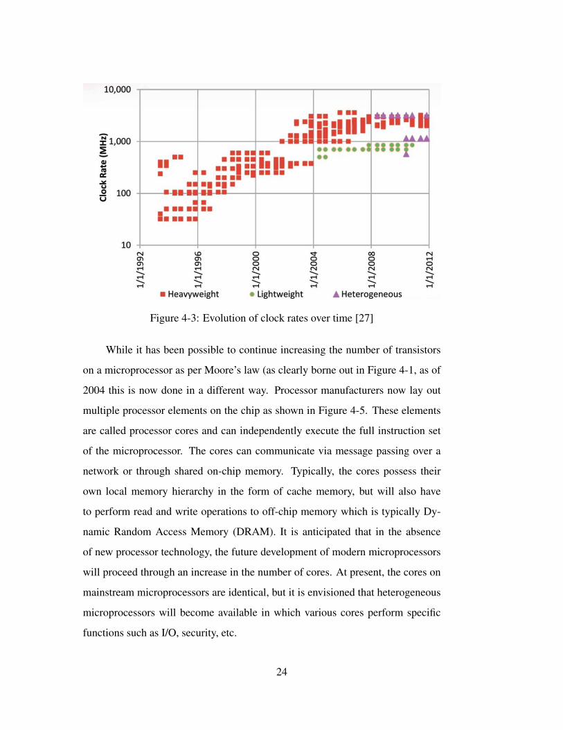
Figure 4-3: Evolution of clock rates over time [27]

While it has been possible to continue increasing the number of transistors

on a microprocessor as per Moore’s law (as clearly borne out in Figure 4-1, as of

2004 this is now done in a different way. Processor manufacturers now lay out

multiple processor elements on the chip as shown in Figure 4-5. These elements

are called processor cores and can independently execute the full instruction set

of the microprocessor. The cores can communicate via message passing over a

network or through shared on-chip memory. Typically, the cores possess their

own local memory hierarchy in the form of cache memory, but will also have

to perform read and write operations to off-chip memory which is typically Dy-

namic Random Access Memory (DRAM). It is anticipated that in the absence

of new processor technology, the future development of modern microprocessors

will proceed through an increase in the number of cores. At present, the cores on

mainstream microprocessors are identical, but it is envisioned that heterogeneous

microprocessors will become available in which various cores perform specific

functions such as I/O, security, etc.

24

Figure 4-4: Evolution of Moore’s law. The top curve shows the total numberof transistors on a microprocessor as a function of time and the trend continuesto follow Moore’s law. The second curve shows that clock speed has flattened.The third curve indicates that this was done to keep power levels low enoughfor cooling purposes. The final curve shows instruction level parallelism becauseclock speeds have flattened, instruction level parallelism has also flattened [34].

4.2 Evolution of Memory Size and Memory Bandwidth

While the number of cores on each processor is increasing, the amount of to-

tal memory relative to the available computational capability is decreasing. This

is a curious measure, but relates to how much memory is available for a given

performance level. In the past, memory technology scaled in a similar way to

processor capability, and so it was possible to provision one byte or more of avail-

25

Figure 4-5: A view of Moore’s law showing evolution of the number of cores ona processor (bottom curve) [21].

able memory for each flop of processing capability. At around the same time as

the transition to multi-core architecture, the ratio of available bytes to flops began

decreasing. This is shown in Figure 4-6. Prior to 2004, the memory size was com-

parable to the number of flops and the ratio of bytes to floating point capability as

measured in flops hovered around and in some cases exceeded one. As of 2004,

the ratio dropped (note that the figure uses a log scale) and is now edging close

to 0.1 for heterogeneous (i.e. multi-core) processor architectures. If this trend

persists (and with current technology it is expected to worsen), it will have an im-

portant impact on the type of applications which can be run on machines that use

traditional DRAM. We discuss this further in Section 5.

Memory capacity using traditional DRAM technology turns out to be a mat-

ter of cost. As shown in Figure 4-7, the cost of memory has not been decreasing

as rapidly as the cost of floating point performance. From the point of view of

26

Figure 4-6: Evolution of the ratio of total memory capacity to floating point per-formance. The vertical axis units are bytes/flop. Prior to 2004 it was possibleto provision 1 byte per flop. Recently this has dropped to less that 0.10 byte perflop [27].

the amount of memory resident on single processor, enormous advances have still

been made. Today, DRAM costs about $5 per gigabyte and so the cost of pro-

visioning say a 32 gigabyte memory for a personal computer is not prohibitive.

However, if one desires a ratio of one byte per flop for an exascale machine, this

will require an exabyte of memory and at today’s costs this is will be $5 B. It is an-

ticipated that while memory costs will decrease, extrapolations using the JEDEC

memory roadmap still indicate a cost of perhaps $1 per gigabyte or more in the

2020 time-frame [53]. As a result, even in 2020 an exabyte of memory will cost

on the order of $1B. Typical budgets for DOE/NNSA high end computer systems

are on the order of $100–200M, and so using current memory technology, it will

only be possible to provision roughly 200 petabytes of memory at best. More

27

Figure 4-7: Evolution of memory cost as a function of time. Also shown is theevolution of floating point cost for comparison. It is seen that floating point costshave decreased far more rapidly [48].

realistically, a memory size of 50 petabytes or so is envisioned.

One might argue that improvements in technology will lead to higher mem-

ory densities and so the 4 GB DRAM of today would evolve into the 1 Terabyte

memory of 2020. Indeed, memory density has increased over time as shown in

Figure 4-8. However, the rate of increase of memory density has never been as

rapid as that of Moore’s law for the number of transistors on a processor. As

shown in the Figure, memory density increased at a rate of 1.33 MBit/chip/year

from 1987 through about the year 2000. Afterwards however, the rate slowed to

0.66 Mbit/chip/year. Today, it is possible to purchase 4Gb on one memory chip.

If current rates of increase hold, it will not be possible to have a terabit memory

chip until perhaps 2034.

28

Figure 4-8: Evolution of memory density as a function of time [48]

Memory bandwidth, or the ability to move data from memory to processor

registers is also a key concern. The memory system associated with a modern

microprocessor is provisioned hierarchically. For processors, one wants rapid in-

struction execution, while for a memory one wants high density to maximize data

available to the processor. As a result, as processors have become more capable

and can execute instructions more rapidly, a performance gap has developed in

that the access times for memory, while decreasing, have not decreased as rapidly

as processor cycle times. This is shown in Figure 4-9. In 1970 the access times

for DRAM and processor cycle times were comparable, but by 1990, as chip de-

signers discovered the benefits of decreasing feature size, lowering voltages, and

increasing clock speed, processor cycle times dropped dramatically. As a result,

the ratio of DRAM access time to processor cycle time began to increase. By

2007, the ratio increased to several hundred to one. Processor designers call this

29

Figure 4-9: An illustration of the von Neumann bottleneck. Processor clock cycletime (blue curve) is plotted over time and compared with DRAM access time(green dashed curve). The ratio of the two is also shown (red dashed curve). Notethat over time the ratio has increased [32].

problem the “memory wall” or the “von Neumann bottleneck”, since it was von

Neumann who first developed the idea of an independent processor that retrieved

its instructions and data from a separate memory.

Processor designers addressed this issue by designing hierarchical memo-

ries to mask the memory latency. In addition to the main memory in the form

of DRAM, modern processors possess memory caches which can store data from

DRAM so that future requests for that data are readily available. Cache memo-

ries located on-chip are typically built from static RAM or SRAM. This type of

memory is constructed from transistors and is very fast, but it has the lowest data

density. It is also more susceptible to radiation induced upsets and so must also

be designed with error correction logic. In contrast, DRAM cells use capacitors

for storage and transistors to move the charge onto an accessed bit-line. This

30

results in a very dense memory, but compromises must be made here too. For

example, memory access produces not just one desired word, but a whole line of

memory which can be a thousand or more words. For these and other reasons,

memory access times from DRAM have not decreased as rapidly. This is not to

say that one could not build a faster DRAM. Indeed there are several promising

approaches such as embedding the DRAM in the processor, or altering the DRAM

core to tailor the amount of data that is retrieved. However, all these concepts im-

pose a penalty on the die size, and, typically, vendors have not embraced these

ideas because providing high memory density is the dominant driver in commod-

ity computers.

Given the hierarchical nature of processor memory, it is preferable to find a

piece of required data in the cache where it can be accessed more rapidly. Data

is transferred to cache from main memory in blocks of fixed size called cache

lines. When the processor needs to read or write a location in main memory, it

first checks to see if the memory address or one associated with the cache line is

available. If the data is present this is called a cache hit. If not, it is a cache miss;

a new entry is allocated in the cache, and the required data is read in from main

memory. The proportion of successful cache accesses is called the cache hit rate,

and this is a measure of effectiveness for the way in which a particular algorithm

utilizes the processor. Processors use caches for both instruction, data and also

address translation.

Cache misses are characterized by how the miss occurs:

Compulsory misses These occur whenever a new piece of memory must be ref-

erenced. The size of the cache or the way the cached data is associated with

main memory will make no difference here. An increased cache block size

can help in this case, as there will then be a higher probability the required

31

data is cached, but this is algorithm dependent. The best approach is to

prefetch the data into the cache. This requires active management of the

cache which is typically left to the compiler. Even prefetching has limits if

a large amount of data is required.

Capacity misses Capacity misses occur because the cache is simply too small. If

one maps the capacity miss rate vs the cache size one can get a feel for the

temporal locality of a piece of data. Note that modern caches are typically

always full and so reading a new line requires evicting an old line of data.

Conflict misses This is a miss that occurred because the required data was al-

ready evicted from the cache. Some of this can also be dealt with through

the provision of larger caches, but because this entails a penalty in terms of

silicon area and performance relative to the provision of functional units, it

is not generally cost effective to increase the cache size.

A cache miss from an instruction cache will cause the most delay as the thread

of execution must halt until the instruction is retrieved. A cache miss from a data

cache may not be as detrimental as instructions that do not depend on the needed

data can be executed instead until the required data arrives. This “out of order”

execution strategy was successful in several processors but is now considered to

be of limited utility because processor speeds have grown faster then memory

access speeds.

4.3 Memory Access Patterns of DOE/NNSA Applications

From the discussion above, it can be seen that the overall performance of a given

application will depend on the amount of memory required to perform the oper-

ations associated with a given algorithm as well as the access pattern associated

32

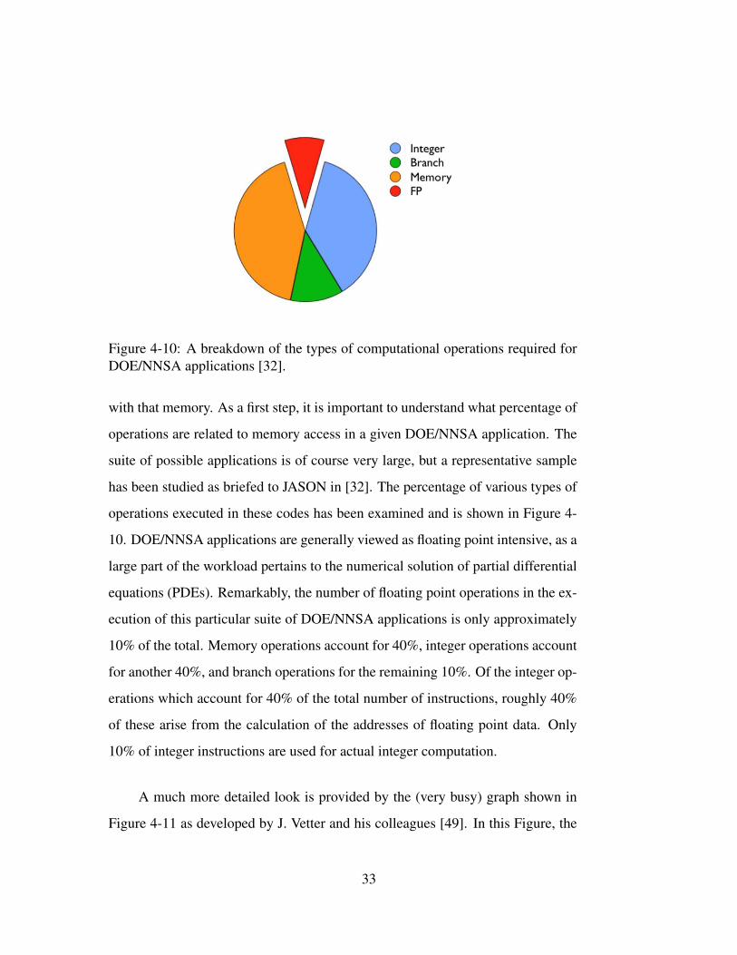
Figure 4-10: A breakdown of the types of computational operations required forDOE/NNSA applications [32].

with that memory. As a first step, it is important to understand what percentage of

operations are related to memory access in a given DOE/NNSA application. The

suite of possible applications is of course very large, but a representative sample

has been studied as briefed to JASON in [32]. The percentage of various types of

operations executed in these codes has been examined and is shown in Figure 4-

10. DOE/NNSA applications are generally viewed as floating point intensive, as a

large part of the workload pertains to the numerical solution of partial differential

equations (PDEs). Remarkably, the number of floating point operations in the ex-

ecution of this particular suite of DOE/NNSA applications is only approximately

10% of the total. Memory operations account for 40%, integer operations account

for another 40%, and branch operations for the remaining 10%. Of the integer op-

erations which account for 40% of the total number of instructions, roughly 40%

of these arise from the calculation of the addresses of floating point data. Only

10% of integer instructions are used for actual integer computation.

A much more detailed look is provided by the (very busy) graph shown in

Figure 4-11 as developed by J. Vetter and his colleagues [49]. In this Figure, the

33

Figure 4-11: Instruction mix for DOE/NNSA applications [49]

34

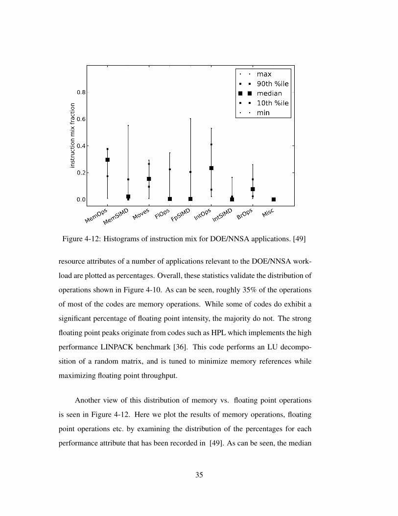
Figure 4-12: Histograms of instruction mix for DOE/NNSA applications. [49]

resource attributes of a number of applications relevant to the DOE/NNSA work-

load are plotted as percentages. Overall, these statistics validate the distribution of

operations shown in Figure 4-10. As can be seen, roughly 35% of the operations

of most of the codes are memory operations. While some of codes do exhibit a

significant percentage of floating point intensity, the majority do not. The strong

floating point peaks originate from codes such as HPL which implements the high

performance LINPACK benchmark [36]. This code performs an LU decompo-

sition of a random matrix, and is tuned to minimize memory references while

maximizing floating point throughput.

Another view of this distribution of memory vs. floating point operations

is seen in Figure 4-12. Here we plot the results of memory operations, floating

point operations etc. by examining the distribution of the percentages for each

performance attribute that has been recorded in [49]. As can be seen, the median

35

fraction for memory operations is at roughly 35%, indicating half of the surveyed

applications exhibit memory access intensities at 35% or more. The situation for

floating point operations is even more striking. The median for both floating point

operations and floating point single instruction multiple data (SIMD) operations is

quite low. Thus the applications associated with the DOE/NNSA workload require

significant memory references relative to floating point and so their performance

is very sensitive to the characteristics of the memory system such as memory

bandwidth. This occurs for several reasons. Compilers are not always able to

optimize floating point throughput without assistance from the programmer. In

addition work is required on the organization of the data flow of the applications

so as to understand if alternate approaches can lead to better performance. We

discuss this further in Section 4.4.

Because of the hierarchical nature of the memory system on a modern mi-

croprocessor, there is a significant performance penalty if a required piece of data

is not available in the various caches of the microprocessor. In this case, the data,

in the form of a cache line, must be requested from main memory, and if no other

productive work can be performed while this access takes place, the processor

will stall. An interesting study of this issue was undertaken by Murphy et al. [33],

who examined the the implications of the working set size on the design of super-

computer memory hierarchies. In particular, they compared the working set sizes

of the applications in the Standard Performance Evaluation Corporation (SPEC)

floating point (FP) benchmark suite to that of a set of key DOE/NNSA applica-

tions run at Sandia National Laboratories. The type of computations performed by

these applications are quite typical of the workload associated with DOE Science

applications as well as NNSA stewardship applications. They include

36

• LAMPPS – a classical molecular dynamics code designed to simulate ato-

mic or molecular systems,

• CTH – a multi-material large deformation shock physics code used at San-

dia to perform simulations of high strain rate mechanics, and

• sPPM – a simplified benchmark code that solves gas dynamics problems in

3D by means of the Piecewise Parabolic Method [11].

The methodology used in this study is to extract an instruction stream of

about four billion instructions from each of these codes. Care was taken to ensure

that the instructions were associated with the core computational aspects of each

of the applications. To determine the working set miss rate of a given applica-

tion, the authors simulated a 128 MB fully associative cache using a least recently

used (LRU) cache eviction strategy. During each load or store operation in the

instruction stream, the cache list is searched for the requested word address. If the

entry is found (a hit) a hit counter for that block is incremented. That entry is then

promoted to the head of the cache list so that it becomes the most recently used

item. By varying the working set size, that is, the list of cache entries, it is possible

to examine the memory requirements for a given application. Note that this ap-

proach measures what is called the temporal working set size miss rate; miss rates

here refers only to temporal locality as opposed to spatial locality. It is possible

that more sophisticated caching or prefetch schemes that take spatial locality into

account could reduce miss rates. As the working set size increases, the probability

that the required datum will be found increases, and the miss rate decreases. But it

will eventually plateau at a level where further increases in working set size (up to

128 million blocks) will not reduce the miss rate, and when this point is reached

one is measuring the compulsory miss rate. In this case, the required data for this

maximum working set size must be fetched from main memory.

37

Figure 4-13: A measure of the bytes required per flop for a variety of Sandiaapplications. Note that the vertical axis label of bytes/flop now refers to requiredmemory bandwidth [33].

Once the miss rate and flop rate are measured, it is possible to infer a memory

bandwidth requirement by dividing the cache miss rate by the number of flops

required to perform a given computation. This byte to flop ratio1 is indicative of

the memory bandwidth required. For example, if this rate is less than one, then less

than one byte per flop must be accessed from main memory. This is a favorable

situation for a modern microprocessor, because it indicates the computation has

high arithmetic intensity; there is significant use (and reuse) of the bytes accessed

from memory into the caches. In this case, we can expect the floating point units

to perform at near optimum rate. On the other hand, if this ratio is greater than one

then it implies that the computation will be limited by the bandwidth associated

with access from main memory. The results for the Sandia applications are shown

in Figure 4-13. It can be seen that even with a cache size of 128M words, the byte

1Not to be confused with the memory capacity to flop ratio discussed earlier.

38

to flop ratio never goes below one. For applications that perform regular memory

accesses like sPPM or CTH, we see that, eventually, we hit a plateau of 3-4 bytes

per flop. But this only happens at a cache size of 100 kB or so. Modern level

1 caches are typically 64 kBytes in size. Level 2 caches are generally bigger, up

to several megabytes. On a typical multi-core processor, however, only a level 1

cache is available to each core. Access to caches at level 2 and above takes place

via a shared memory bus.

We emphasize that this analysis is not definitive for two reasons. First, it does

not completely take into account the role of prefetching of data from memory to

a level 2 cache. Secondly, the binaries that are run in this analysis are not hand-

optimized, and it may be possible to improve this byte to flop ratio by applying

techniques to manage cache affinity. The authors in reference [33] also applied

this analysis to the SPEC-FP benchmark and showed that the byte/flop ratios for

these applications are smaller than those for the Sandia suite. One can conclude,

therefore, that the DOE/NNSA workload may require greater memory bandwidth

than conventional floating point intensive applications, but this requires further

systematic assessment. A more quantitative view of the memory bandwidth issues

is presented in the next section.

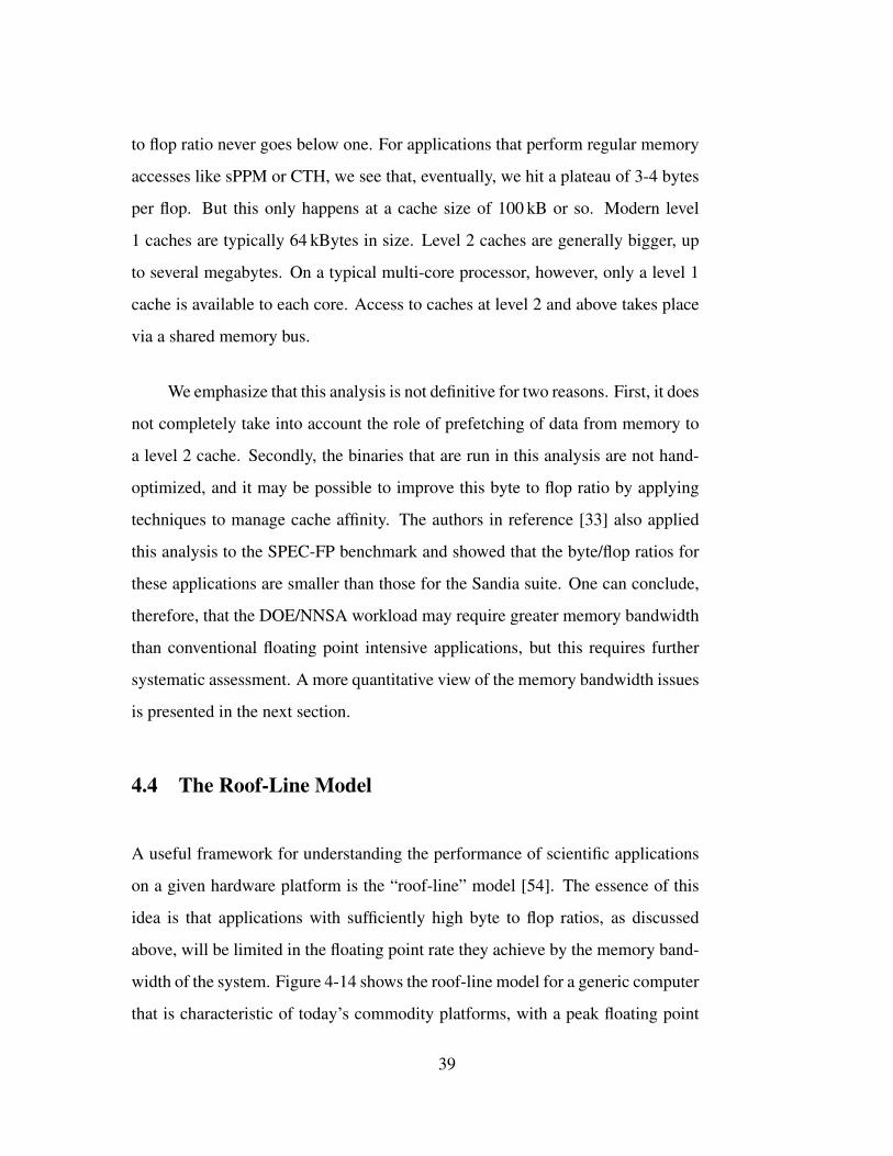
4.4 The Roof-Line Model

A useful framework for understanding the performance of scientific applications

on a given hardware platform is the “roof-line” model [54]. The essence of this

idea is that applications with sufficiently high byte to flop ratios, as discussed

above, will be limited in the floating point rate they achieve by the memory band-

width of the system. Figure 4-14 shows the roof-line model for a generic computer

that is characteristic of today’s commodity platforms, with a peak floating point

39

1/16 1/8 1/4 1/2 1 2 4 8 16 32arithmetic intensity [flop/byte]

101

102

floati

ng p

oin

t perf

orm

ance

[G

flop/s

]

mem

ory

band

wid

th-li

mite

d

peak flop rate

Figure 4-14: Roof-line model for a generic 2012 commodity computer, with 100Gflop/sec peak floating point performance, and 20 Gbyte/sec memory bandwidth.The solid curve represents the maximum achievable floating point performance ofan application as a function of its arithmetic intensity (flops-to-byte ratio). Below5 flop/byte, an application is memory bandwidth-limited, as shown by the slopedline. Above 5 flop/byte, an application can achieve the peak floating point per-formance provided by the CPU. The dashed line shows a hypothetical scientificapplication at an arithmetic intensity of 0.5.

capability of 100 Gflop/sec, and a peak memory bandwidth (between DRAM and

CPU) of 20 GB/sec. Plotted in the figure is the maximum achievable floating point

performance as a function of the arithmetic intensity (flop-to-byte ratio, where

“byte” refers to a byte of memory read from DRAM) of an application running

on this hardware. 2 At high arithmetic intensity (> 5), there is sufficient memory

bandwidth to keep the processor fed, so the peak floating point rate of the CPU is

achievable. At low arithmetic intensity (< 5) there is not enough memory band-

width to keep the floating point units busy, so the maximum achievable floating

2Note, the following discussion uses the metric of flops to bytes rather than bytes to flop. Theformer is the right metric to use when there is good reuse of cache data.

40

1/16 1/8 1/4 1/2 1 2 4 8 16 32 64 128arithmetic intensity [flop/byte]

101

102

103

floati

ng p

oin

t perf

orm

ance

[G

flop/s

]

today

2020 (pro

jecte

d)

Figure 4-15: Roofline model for a generic commodity computer in 2020 (solidline) and 2012 (dashed line). Memory bandwidth is assumed to double every3 years, while floating point performance is assumed to double every 1.5 years.Note that the ridge point moves from 5 flop/byte to 32 flop/byte.

point rate is limited by the memory bandwidth, as indicated by the sloped line.

The point on this figure where the memory bandwidth-limited floating point rate

meets the peak floating point rate is known as the “ridge point,” and occurs at

an arithmetic intensity of 5 for this generic processor. In other words, to reach

peak floating point performance on this hardware requires an application that can

perform 5 floating point operations for every byte of memory read from DRAM.

Scientific applications of interest to DOE or NNSA span a range in arithmetic

intensity, but rarely have intensities above 1 [33]. The optimistic value of 0.5 is

shown in the figure as a vertical line. For such an application on this hardware, the

maximum achievable floating point performance is merely 10 Gflop/sec, a factor

of 10 below the peak performance of the CPU of 100 Gflop/sec.

41

There is every indication that the trend of CPU performance doubling ev-

ery 18 months (via Moore’s Law) [31] will continue; as indicated previously, this

performance increase is realized today by an increase in the number of proces-

sor cores instead of an increase in the performance of an individual core, but

this detail is not relevant to the current discussion. The trend for memory band-

width improvement, however, has been the subject of much less focus. Over the

past decade, memory bandwidth to CPU has doubled approximately every 3 years

[38], and current indications are that the growth rate will decrease absent new

developments.

Making the optimistic assumption that memory bandwidth trends will con-

tinue (at a doubling every 3 years), and assuming that CPU performance will

continue to follow Moore’s Law, we plot in Figure 4-15 the roof-line model for

a commodity system in 2020. For reference, we include the roof-line model for

today’s hardware as the dashed line. By 2020, CPU performance gains will have

outpaced memory bandwidth gains to such a degree that to reach peak floating

point performance on our representative system will require something like 32

flops per byte in arithmetic intensity! Our reference application with an arithmetic

intensity of 0.5 will reach a mere 63 Gflop/sec in floating point performance on a

CPU capable of a peak floating point rate of 4 teraflop/sec. This corresponds to

an efficiency of only 1.5%!

Yelick and her colleagues at Berkeley have applied the roof-line model to

DOE/NNSA applications [57]. In Figure 4-16, we show the roof-line curve for

the Intel Xeon 550, a commercial processor used in workstations and servers. The

Xeon processor has a peak speed of about 256 gigaflops per second using single

precision arithmetic. The memory system for this processor is such that it requires

an arithmetic intensity of about 4 flops per byte in order to realize this peak per-

42

Figure 4-16: Roofline results for the Xeon processor [57].

formance. The colored regions correspond to several types of applications that

use the same computational patterns as DOE/NNSA applications. For example

“SpMV” in the Figure stands for a sparse matrix vector multiply, an operation

that is relevant for example to finite element analyses. As can be seen, the ef-

ficiency for this pattern is quite low, ranging from 2 gigaflops at the low end to

8 gigaflops at the high end; the memory bandwidth achieved is quite low, with

a flops to byte ratio less than one in all cases. This is to be contrasted with the

DGEMM application corresponding to a full matrix-matrix multiply. This corre-

sponds to a different computational pattern, and the algorithms for matrix mul-

tiplication of full matrices allow for significant reuse of cached data. This type

of calculation is often used to characterize the peak floating point performance of

a modern processor. The other colored regions represent applications that have

computational patterns that do not perform optimally given the roof-line limits,

presumably because traditional memory caching strategies are inadequate.

43

Figure 4-17: Roof-line results for the Nvidia Fermi processor [57].

In Figure 4-17 we show the same roof-line curve but for a modern graphics

processing unit (GPU), the NVIDIA Fermi C2050. A GPU can provide significant

performance improvements over a traditional processor provided the flop to byte

ratio is sufficiently high. For example, the dense matrix-matrix multiply is accel-

erated by almost a factor of four over the Xeon processor. In contrast, applications

like the sparse matrix-vector multiple do not show appreciable speed-up. Again,

the issue is to be able to either cache memory effectively or apply an application-

specific prefetching strategy that can hide the latency of the required memory

accesses.

Extrapolating current trends, it is clear that commodity hardware is chang-

ing in a way that will continually reduce the efficiency of existing science appli-

cations. The question, of course, is “What can be done?”. The roof-line model

shown in Figure 4-15 suggests possible solutions. Since processors are currently

44

limited in terms of memory bandwidth, and will certainly be so in 2020, one

could imagine attempting to influence vendors to design higher bandwidth CPU–

DRAM interconnects. One difficulty faced here is that memory bandwidth is ap-

proximately proportional to the number of leads coming from the CPU package,

and we are currently facing physical constraints in increasing this number. An-

other difficulty with increasing memory bandwidth, as we discuss below, is that

the energy cost to move data (the dominant energy cost in scientific calculations)

at exascale may greatly exceed a reasonable power budget.

Another possible solution suggested by Figure 4-15 is to increase the arith-

metic intensity of DOE/NNSA science applications. This can be achieved in one

of two ways. First, by optimizing and tuning a code, one can sometimes increase

the flops-to-byte ratio without changing the underlying algorithm. This typically

takes the form of structuring memory accesses to increase the cache hit rate, and

usually leads to modest increases in arithmetic intensity, although, to our knowl-

edge, a thorough study of the potential for this approach has not been under-

taken for DOE/NNSA applications. In Section 7, we describe some techniques

for automating and simplifying this process. The second method for increasing

the flops-to-byte ratio is to modify the underlying algorithm itself. This may be

possible in some cases, but the path forward is not clear for all applications as-

sociated with the DOE/NNSA workload. This is clearly a research priority. It is

interesting to note that the development of capable hardware can make it possible

to use algorithms which were previously not thought to be suitable. For example,

while the idea of the fast Fourier transform (FFT) was understood some time ago

(possibly by Gauss), it was only the invention of the digital computer which made

it a revolutionary advance as pointed out by Cooley and Tukey [13].

45

Although our discussion of hardware so far has been kept rather simplified,

it should still be clear that the scaling trends do not favor scientific applications if

the flops to byte ratios are indeed as low as indicated in the previous section.

4.5 Energy Costs of Computation

An additional major technical issue in realizing exascale computing is the cost

of energy for computation. It is not hard to see that energy cost is a potentially

significant issue. For example, the IBM BG/P computer recently installed at the

Lawrence Livermore Laboratory achieves a LINPACK benchmark speed of 16

petaflops and uses roughly 8 megawatts of power. If one envisions achieving an

exaflop by simply scaling up this technology, such a computer would require 400

megawatts to operate. At current rates for power this would cost $400M per year

assuming it were possible to deliver 400 megawatts to the data center housing the

computer.

Shown in Figure 4-18 are the energy costs of various basic operations as

measured in picoJoules on a 64 bit word. The gray curve represents the energy

costs today. The blue curve represents projected energy costs for these operations

in 2020. For example, a double precision floating point operation today requires

about 25 pJ of energy. By 2020, as feature sizes for microprocessors shrink fur-

ther, it is expected that such an operation will require only 4 pJ. The costs for

register access are even less, and the costs for accessing an 8 kB SRAM are com-

parable. This is because all such operations take place close to the functional units

of the processor, and as mentioned earlier, SRAM memory is built from transistors

and is designed for rapid access, but has low density relative to DRAM.

46

Figure 4-18: Energy costs for computational operations. Vertical axis labels de-note picoJoules. All costs are for operations on a 64 bit word [26].

Other operations that require communication over the processor must factor

in the cost of signaling plus the cost of performing the operation. For example to

communicate a 64 bit word over a distance of 1 mm across the chip costs roughly

8 pJ per mm of distance. This is due to the resistance that must be overcome in

performing the signaling. Note too that while a factor of six reduction in energy

use is projected for floating point operations by 2020, a more modest factor of two

improvement is projected for communication across the chip.

Finally, there is a very large disparity between the energy costs of floating

point computation and off-chip memory access. Today, a DRAM access for 64

bits requires 1.2 nJ and this may decrease by a factor of 4 to 320 pJ by 2020. The

ratio of energy costs between memory access and floating point today is about 50

to 1 today but is projected to increase to 80 to 1 by 2020.

47

While the energy costs of individual operations seem quite modest, they be-

come substantial when one contemplates building an exascale computer. A power

utilization rate of 1 pJ per second translates into a utilization rate of 1 MW per sec-

ond if one simply scales up to the exascale. Because the power budget for most

modern data-centers is on the order of 20 MW the provision of hardware resources

for an exascale machine is constrained not only by technological issues but also

by energy utilization.

4.6 Memory Bandwidth and Energy

The memory bandwidth issue is largely one of energy, and, to a lesser extent, pin

constraints. Accessing DRAM today requires about 30 pJ/bit, so a 200 GB/sec

(1.6 Tb/sec) memory system on a single GPU node consumes about 50 W. This is

divided three ways between row activation (bit-line energy), column access (on-

chip communication from the sense amps to the pins of the DRAM), and I/O

energy (off-chip communication).

There are techniques that can reduce all three components of energy. Row

activation energy is high because each row access reads a very large (8K-bit)

page. Reducing the page size will linearly reduce this component of energy. For

example, using a 256 B page size will save a factor of 32 on row activation with

little downside. Column access energy can be reduced by more efficient on-chip

communication. On-chip communication energy is currently about 200 fJ/bit/mm

and circuits have been demonstrated operating at 20 pJ/bit/mm. Finally off-chip

communication using the single transmission line (STL) signaling standard used

in DRAM takes about 20 pJ/bit (2/3 of the total energy) and signaling systems

with 1-2 pJ/bit have been demonstrated. Based on expected improvements, one

can expect total access energy for commodity memory to drop to the 5-10 pJ/bit

48

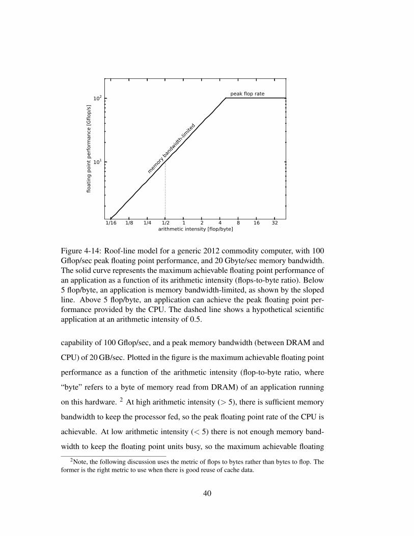
Table 4.2: Some point designs for an exascale computer. These estimates usethe energy costs of DRAM access and floating point computation and assume theprocessing of the full memory capacity of the machine.

range by 2020.

With today’s DRAM costs and a power budget of 50–75 W for DRAM ac-

cess, one is limited to 200–300 GB/sec bandwidth. With a drop to 10 pJ/bit in 2020

the energy limit on bandwidth will be 600–900 GB/sec. Pin bandwidth is also a

limiter here. One can place 512-1K channels per chip and run them up to 20Gb/sec

(perhaps 40Gb/sec by 2020) so the pin bandwidth limit is 1.2–2.4 TB/sec today

and is expected to be 2.4–4.8 TB/sec by 2020. With both today’s technology and

expected scaling, energy is a bigger limiter than pin bandwidth. Also, one can

overcome the pin limit by splitting a processing chip into several smaller chips.

To first approximation, the pin bandwidth per chip, which is limited by the escape

pattern, under the package remains constant.

49

4.7 Some Point Designs for Exascale Computers

Using the energy and cost estimates discussed above, it is possible to make rough

estimates of the power requirements for exascale platforms. Table 4.2 uses the

memory cost figures in Section 4.2 and the energy figures in the previous section

to compute rough power costs and memory costs for various configurations of an

exascale system.

One can, in fact, design an exascale system today that has no memory, but

provides enough floating point units for an exaflop. Such a machine would have

little utility, but can be considered an (extreme) bounding case. Using the esti-

mates above, such a machine would still require 25 MW to power and so could

not be built today within a power budget of 20 MW, but could be built in 2020 and

would be comfortably within the power budget. If we then ask that the machine

provide about 1 byte per flop, we find that cost is an issue as the memory cost

alone would be $1 B. Power will also be an issue as the cost of communicating an

exabyte of memory to match the flop rate would require an additional 40 MW in

2020. If an application can efficiently reuse the data accessed from main memory,

then the power requirements are lessened, since in the same period we do not have

to access memory as frequently. In this case, we get close to the power require-

ments of 20 MW while maintaining a byte of memory per flop. However, memory

costs for such a system are still prohibitive.

If one reduces the memory capacity so that the memory to flop ratio is 0.1 (a

memory of 100 Petabytes) then memory costs become more reasonable although

still quite high. Such a system would also dissipate less power in that a factor

of 10 less energy is required to access the entire memory. If the accessed mem-

ory can be productively cached, and a ratio of 1 byte to 1 flop can still produce

50

Figure 4-19: Power projections for exaflop computing. A variety of assumptionsare employed to extrapolate power utilization of HPC platforms to the 2024 time-frame. Further details of this assessment may be found in [32]

reasonably sustained performance from the floating point units, then this system

is well within our power requirements of 20 MW. However, if we look at current

implementations of DOE/NNSA applications as described in Section 4.3 we see

that the byte to flop requirements are more like 3-5 bytes per flop. In this case, the

energy requirements do increase and eventually exceed our 20 MW limit.

Our crude estimates are roughly in line with more sophisticated estimates

outlined in the 2008 DARPA report [27]. In Figure 4-19 we show the energy per

flop as measured in present day architectures as well as the extrapolation to future

years. Recall that one must be able to bring the total cost for an flop of computing

to 20 pJ in order to stay within the 20 MW power envelope. The dots indicate

current measurements of various types of present day architectures:

51

Heavyweight These architectures use high power CMOS; an example is the Cray

Red Storm machine which uses Opteron processors,

Lightweight A typical lightweight architecture would be the IBM BlueGene ma-

chines which use low power CMOS,

Heterogeneous This type of architecture is typified by the Los Alamos Road-

runner machine which uses accelerators based on IBM’s cell processor to

accelerate floating point intensive tasks. Another example would be hybrid

machines that use GPU’s attached to general purpose compute nodes.

As can be seen the heterogeneous machines have been the most power effi-

cient to date as they can make use of hardware optimized for throughput of data

to the floating point units. It is anticipated that these types of architectures are the

most promising in terms of projections of future power usage, but it can be seen

that even for these, the achievement of energy utilization of 20 pJ per flop may not

occur until 2024.

4.8 Resilience

In this section, we examine some of the salient issues associated with the resilience

of HPC systems. Recent reports show that hardware errors are the dominant cause

of system failures in modern HPC machines [27, 42]. As an example, Figure 4-20

shows a breakdown of root causes for system failures (both soft and hard) seen

in the LANL HPC systems observed by [42] over a period of a few years. For

these systems, hardware errors account for roughly 2/3 of all system failures. The

components that tend to fail most in HPC machines are RAM and CPUs [27]. For

example, failure predictions for BlueGene/L anticipated roughly 60% of system

failures would be caused by RAM, and approximately 25% would be caused by

52

questions are 1) whether the root cause breakdown changesover the lifetime of a system and 2) how it varies across thedifferent types of systems at LANL.

Regarding question 1, we do not see a significant changein the root cause breakdown over the lifetime of a system(i.e., when moving from initial deployment to later years ofoperation). The main change we observe is that for somesystems, the percentage of failures with unidentified rootcause drops over time. However, the relative frequency ofthe other types of failures remains unchanged.

Regarding question (2), Fig. 2a shows root causeinformation broken down by the type of system. Each ofthe five bars to the left presents the breakdown across allfailure records for systems of a particular hardware type.2

The rightmost bar describes the breakdown across allfailure records in the data set.

Fig. 2a indicates that while the basic trends are similaracross system types, the actual breakdown varies. Hard-ware is the single largest component for each system type,with the actual percentage ranging from 30 percent to morethan 60 percent. Software is the second largest contributorfor each system type, with percentages ranging fromfive percent to 24 percent. Type D systems differ mostfrom the other systems, in that hardware and software arealmost equally frequent as a root cause.

We asked LANL about the higher fraction of downtimewith unknown root cause for systems of type D and G andwere told the reason lies in the circumstances surroundingtheir initial deployment. Systems of type G were the first

NUMA-based clusters at LANL and were commissionedwhen LANL had just started to systematically recordfailure data. As a result, initially the fraction of failureswith unknown root causes was high (>90 percent), butdropped to less than 10 percent within two years, asadministrators gained more experience with the systemand the root cause analysis. Similarly, the system of type Dwas the first large-scale SMP cluster at LANL, so initiallythe number of unknown root causes was high, but thenquickly dropped.

The above example shows that interpreting failure dataoften requires interaction with the people who run thesystems and collect the data. The public release of the data[1] includes a complete FAQ of all questions that we askedLANL in the process of our work.

We also study, using the repair time information in theLANL data, how much each root cause contributes to thetotal repair time. Fig. 2b shows the total downtime persystem broken down by the downtime root cause. The basictrends are similar to the breakdown by frequency: hard-ware tends to be the single largest component, followed bysoftware. Interestingly, for most systems, the failures withunknown root cause account for less than 5 percent of thetotal downtime despite the fact that the percentage ofunknown root causes is higher. Only systems of type D andG have more than 5 percent of downtime with unknownroot cause.

In addition to the six high-level root cause categories inthe LANL data (recall Fig. 2), we also looked at the moredetailed root cause information. Table 3 shows the 10 most

340 IEEE TRANSACTIONS ON DEPENDABLE AND SECURE COMPUTING, VOL. 7, NO. 4, OCTOBER-DECEMBER 2010

Fig. 2. The breakdown of failures into root causes (a) and the breakdown of downtime into root causes (b) for the LANL systems. Each graph showsthe breakdown for systems of type D, E, F, G, and H and aggregate statistics across all systems (A-H).

2. For better readability, we omit bars for types A-C, which are smallsingle-node systems.

Fig. 1. The breakdown of failures into root causes for the LANL systems (a) and system X (b). The LANL graph shows the breakdown across all

systems (A-H).

Figure 4-20: Breakdown of root causes for system failures seen in the LANL HPCsystems observed by [42] over a period of a few years.

either CPUs or I/O ASICs [27]. Although RAM failures tend to outweigh CPU

failures in the statistics reported in the literature, we note that there is a selection

effect at work, since ECC-enabled RAM can detect and report errors, while CPUs

are generally not designed to do so.

Hardware errors can be broadly categorized into three classes [12]: transient,

intermittent, and permanent. Transient errors are those that are due to the envi-

ronment. At sea level, neutrons induced by cosmic rays are thought to be the

primary culprit, but alpha particles emitted by radioactive impurities in the elec-

tronics packaging may also play a role. Intermittent errors are those caused by

marginal or failing hardware. In a typical scenario, a key parameter of a device,

through aging, drifts in value and eventually exceeds the device’s built-in margin.

One well-known example in the electronics industry is the negative bias tempera-

ture instability, in which the threshold voltage of a MOSFET increases with time.

A more pedestrian, though very relevant, failure mode is the intermittency of con-

tacts at solder joints. Permanent errors are, just as the name implies, irreversible

53

physical changes that render a device inoperable and may be the eventual fate

of some intermittent errors, although they can also be caused by some extreme

environmental conditions.

Although there is a rich literature on the classification, detection, and causes

of hardware errors, it is still not clear exactly what causes the errors seen in HPC-

class machines. Although attempts have been made to assess the extant data 3,

raw failure data is sparse. In addition, when failures are recorded, the root cause

is often not known (although see [30] for an exception to this rule).

At the component level, however, some trends can be discerned. Transient

failures in CPUs are thought to be caused primarily by cosmic ray-induced neu-

trons which, when they strike a silicon nucleus, produce charged secondary frag-

ments. Those secondary fragments in turn generate excess electron-hole pairs. If

those electron-hole pairs are near a p–n junction, the electric field will separate

them, leading to a change in voltage. If the voltage is above threshold, an error

results [47]. Since the cosmic ray-induced neutron flux is approximately constant

over time-scales of months, the error rate should scale with the quantity of silicon

in a chip. The scaling with voltage is more complex, but it has been shown that

the failure rate increases with decreasing voltage [23]. Since the area of processor

chips is now roughly constant with time, and core voltages appear to be leveling

off, the transient failure rate for CPUs should be approximately constant across

generations. This result is in fact consistent with the rule of thumb presented in

[27] that the system failure rate scales with the total number of sockets. An inter-

esting consequence is that as the number of cores per CPU chip is increasing, the

failure rate per core should in fact decrease over time. As with CPUs, the failure

rates of RAM modules should scale with the quantity of silicon. Some reports

3see, e.g., the Computer Failure Data Repository http://cfdr.usenix.org

54

indicate that the failure rate per DIMM has not increased across generations [41].

Adopting the [27] rule of thumb that the system failure rate scales with the

socket count, we can predict future system-level failure rate trends. For clarity

of exposition, we will explore two hypothetical exascale systems: one in which

RAM causes all system failures, and one in which CPUs cause all system failures.

The reason for the simplification is that memory density and CPU performance

scale differently with time as indicated previously. In addition, combining the two

in a mathematical model is not particularly insightful. We will take the LANL

Roadrunner computer as our reference system, with a birth date of 2008, and

with a peak performance we define as 1 petaflop (factors of two are irrelevant

here). Transistor count doubles every 2 years for CPUs which, as pointed out

previously, means core count per CPU doubles every 2 years. Adopting 2020 as

our target date for an exascale system, we find that in the 12 years from 2008

the core count per CPU should increase by a factor of 212/2 = 64. Requiring

floating point performance that is 1000× that of Roadrunner will thus require

1000/64 ≈ 16 times as many CPUs and, consequently, 16 times as many CPU

sockets. The growth of socket count for high performance computers over time is

shown in Figure 4-21. The failure rate of such a system would be 16 times higher

than that of one of today’s petascale machines. For example, if a current petascale

machine has a reasonable mean time to system interrupt (MTSI) of 64 hours, an

exascale machine would have an MTSI of merely 4 hours!

We turn now to an exascale machine with 1000× the memory capacity of

Roadrunner (even though such a system may be infeasible for other reasons, as

described in Section 6). Recent trends show memory density doubling every three

years [3]. By 2020, memory density will have increased by a factor of 212/3 = 16.

Requiring 1000× the memory capacity of Roadrunner will require the number of

55

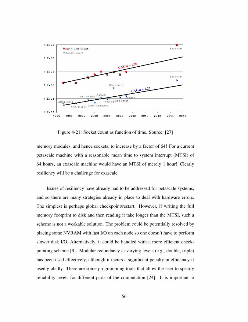
Figure 4-21: Socket count as function of time. Source: [27]

memory modules, and hence sockets, to increase by a factor of 64! For a current

petascale machine with a reasonable mean time to system interrupt (MTSI) of

64 hours, an exascale machine would have an MTSI of merely 1 hour! Clearly

resiliency will be a challenge for exascale.

Issues of resiliency have already had to be addressed for petascale systems,

and so there are many strategies already in place to deal with hardware errors.

The simplest is perhaps global checkpoint/restart. However, if writing the full

memory footprint to disk and then reading it take longer than the MTSI, such a

scheme is not a workable solution. The problem could be potentially resolved by

placing some NVRAM with fast I/O on each node so one doesn’t have to perform

slower disk I/O. Alternatively, it could be handled with a more efficient check-

pointing scheme [9]. Modular redundancy at varying levels (e.g., double, triple)

has been used effectively, although it incurs a significant penalty in efficiency if

used globally. There are some programming tools that allow the user to specify

reliability levels for different parts of the computation [24]. It is important to

56

continue work on software-based mitigation measures to deal with intermittent

system failures. However, it is also important that a systematic investigation be

undertaken to uncover the root causes of the hardware failures observed in HPC-

class machines, and work with vendors to increase hardware reliability.

We describe some potential hardware-based mitigation measures for tran-

sient errors. If further DOE-supported investigation reveals that, as expected, cos-

mic ray-induced neutrons are the dominant source of transient errors, there are

avenues to be explored. The cosmic ray flux varies by a factor of ∼ 2 from the

Earth’s equator to the poles [58]. Locating a compute cluster in Miami instead of

Albuquerque, although perhaps an unpopular decision, would reduce the transient

error rate by approximately one third. The cosmic ray flux also varies with altitude

(as ASC Q showed). Locating installations at low altitudes or underground would

decrease the error rate. Neutron shielding (e.g., concrete, polyethylene) could also

placed around a compute cluster to reduce neutron flux exposure. Vendors typi-

cally perform simulations and experiments to characterize hardware errors [45].

DOE could attempt to influence vendors early in the design phase to produce more

error-resistant hardware. This could be realized by adding ECC to chip compo-

nents or, in some cases, modifying the chip design.

4.9 Storage

We describe here some of the issues associated with archival storage for an exas-

cale machine. There are several challenges here. First, check-pointing of the data

to archival storage has to be done in a different way than currently performed. The

time taken to checkpoint may exceed the MTSI of the machine and so some sort

of intermediate buffering (a burst buffer) must be considered. Second, the very

size of the required disk array will further exacerbate the power utilization issues

57

discussed previously. As a result, the archival facility may have to be operated in

a rather different way with many of the disks spun down most of the time. Finally,

there is the issue of data loss and retention due to disk failure.

4.9.1 Density

Currently, the capacity of hard disk drives ranges from less than 300 GB (for high-

end “Enterprise Class” storage) to 3 TB (for consumer-grade storage), with a rel-

atively slow growth in areal density of 20–25% per year [16]. Previously, the

storage industry had enjoyed some years of more than 100% growth in areal den-

sity per year, which accompanied the introduction of the Giant magnetoresistance

(GMR) read head, but subsequent gains have been more difficult. The industry has

moved from longitudinal to orthogonal recording, as well as to harder magnetic

materials. There is a significant challenge in writing the magnetic media since

the field required to write the materials with a smaller domain size is difficult to

contain and could affect adjacent domains. A proposal to do what is called shin-

gled recording [2] is expected to yield an increase in density by a factor of 2–4,

but at the cost of making the hard disk drive no longer a simple random access

device. The expected density gain from shingled recording is also expected to be

short-lived [16].

Increases in areal density require harder magnetic materials in order avoid

thermal instability. Charap’s recognition of the super-paramagnetic effect [8] was

the cause of the most recent large technological shift from longitudinal to orthog-

onal recording. The next large step in recording density is expected to result from

Heat-Assisted Magnetic Recording (HAMR) which uses a laser to heat a small

area in order to reduce its coercivity. An alternative to HAMR that is being inves-

tigated is Microwave-Assisted Magnetic Recording (MAMR), which instead of a

58

laser uses microwaves. HAMR will be required to go beyond more than about

1.3 Tb/in2 with the step beyond HAMR and MAMR being bit-patterned media,

both lithographic and self-organizing are being considered, but this is not expected

until after 2016 [16]. It is believed that areal densities of more than 10 Tb/in2 may

be achieved before bit-patterned media will be required.

Thin film magnetic domains have both a length and a width on the platter

surface; the width is related to the track density, which in turn is a function of

the physical dimensions and the magnetic properties of the the read/write head

and of the control system. Currently, track density is increasing faster than bit

density, resulting in a more square bit aspect ratio. Track density is currently

approximately 400,000 tracks per inch (TPI) as of 2012, and is expected to exceed

700,000 TPI by 2016. There is some concern that engineering difficulties may

limit areal density to below the atomic densities of 10–50 Tb/in2. For example,

a head fly height of 4 nm is required for more than 1 Tb/in2 [16]. But thermal

effects related to super-paramagnetism are of much more immediate concern.

In the 2016 time frame, it is expected that a 12 TB hard disk drive will be

shipped in a 3.5 inch form factor, and 4–5 TB hard disk drive in a 2.5 inch form

factor. A 12 TB hard disk would require 4 platters in a 3.5 inch form factor. It

is unlikely that the number of platters will increase significantly since the form

factor is now a standard and more platters require more energy. If the trend in areal

density continues, then we can expect 24–30 TB hard disk drives to be available

by 2020 in a 3.5 inch form factor.

In order to build a petabyte (1015 bytes) of non-redundant storage using the

current generation of 3 TB hard disk drives, about 333 would be required. An

exabyte (1018 bytes) would require about 333,000 such hard disk drives, and 100

exabyte file system would require about 3,333,000 such disk drives. The expected

59

gains in areal density would reduce this by about a factor of ten by 2020. Per-

formance increases more slowly - approximately as the square root of the areal

density (it is a function of the bit density and the track pitch).

4.9.2 Power

The power profile of hard disk drives is dominated by the energy required to keep

the platters spinning (called rotation), and secondarily by the energy required to

move the read/write head (called seek).

The power consumption of current hard disk drives is given in Table 4.3

for standard 3.5 inch hard disk drives and in Table 4.4 for smaller, lower power

mobile hard disk drives. These tables include pure-write workloads, a streaming

video workload, a mixed read/write workload, and when the disk drive is idle (this

excludes explicit sleep states). A typical consumer-grade hard disk drive such

as the 2 TB Western Digital WD20EFRX consumes approximately 4.8 W while

writing, 3.6 W under a light read workload, and 3.5 W while idly spinning. An

“Enterprise Class” hard disk drive such as the Hitachi Ultrastar 15K300 can store

only 300 GB but spins at 15,000 RPM and consumes approximately four times the

power.

It is unlikely that the platters will spin faster than 15,000 RPM purely for

energy reasons, and it is also unlikely that they will spin slower than 5,400 RPM

for performance reasons. It is important to remember that the data rate that can be

achieved from a hard disk drive is linear in the rotational speed of the platter and

grows as roughly the square root of the areal density (linear in the bit density) of

the recording. As a result, it is unlikely that the data rates will grow much faster

than the square root of the areal density.

60

Table 4.3: Hard disk drive (HDD) power utilization

Power (W)

Model Size RPM Write Read Mixed Idle

WD WD20EFRX 2 TB 5400 4.8 3.6 4.2 3.5

WD WD30EFRX 3 TB 5400 5.4 4.0 4.6 3.9

Hitachi 7K1000 1 TB 7200 10.6 8.5 12.9 8.2

Hitachi 10K300 300 GB 10000 16.4 13.1 15.9 13.4

Hitachi 15K300 300 GB 15000 17.4 14.8 16.2 14.5

Table 4.4: Mobile HD Power Requirements

Power (W)

Model Size RPM Write Read Mixed Idle

Toshiba MK5055GSX 500 GB 5400 2.1 1.2 1.7 0.6

Hitachi 5K1000 1 TB 5400 2.2 0.9 2.1 0.6

Samsung M8 HN-M101MBB 1 TB 5400 2.7 1.1 2.1 0.8

WD Scorpio WD7500BPKT 750 GB 7200 3.4 1.4 2.7 0.9

Seagate Momentus XT 750 GB 7200 3.9 2.1 2.5 0.8

It is instructive to do some back-of-the-envelope calculations in order to get

a lower-bound on the amount of power that will be required. For simplicity, we

consider what is required just to operate the hard disk drives. Let us assume then a

consumer-grade hard disk drive such as the Western Digital WD30ERFX, which

holds 3 TB of data and requires about 5 W for an relatively intense read/write

workload as might be expected in an exascale computer system. The result is

333.33disks/PB× 5W/disk = 1666.67W/PB = 1.67kW/PB. An exabyte then

costs us 1.67 MW, and a 100 exabyte file system costs us 167 MW. A similar

calculation using high-end enterprise class storage requires 3333.33disks/PB×

61

15W/disk = 50kW/PB, 50 MW/PB, and 5 GW for a 100 exabyte file system.

The hard disk drives used in mobile computing are really no better, except

that they have a lower-power idle state. Consider the Hitachi 5K1000, which

holds 1 TB and requires about 1.5 W for a relatively intense read/write workload.

At 1000disks/PB, an exabyte costs 1.5 MW, which is comparable to the power

required by the consumer-grade hard disk drives. We should note that there are

three times as many drives required, and so we are likely to see an improvement

in performance but also an approximately three times higher failure rate for the

system.

Given the projected growth rate of 20–25% in areal density, we can expect

to cut the power requirement for a given amount of storage by a factor of ten. It

is important to note though that if we reduce the number of hard disk drives by a

factor of 10, we will be reducing the performance of the system by approximately

a factor of 3. As a result, using consumer-grade hard disks drives we could expect

to build our 100 EB file system for about 17 MW, not counting the energy required

for the interconnection network which will be substantial. Building the 100 EB

file system using enterprise class storage will still require an untenable 500 MW

of power.

It is also important keep in mind that the data storage system is not simply

a collection of hard disk drives. It also includes processors, memory and an in-

terconnection network. The I/O nodes that comprise a data storage system are

processors with relatively large DRAM memories that are used as caches with

high-bandwidth interconnection networks to the compute nodes (and among the

I/O nodes). The number of hard disk drives per I/O node will depend on the per-

formance requirements of the system, as well as the interconnection technology

employed to the hard disk drives. Depending on the ratio of hard disk drives to

62

I/O nodes, the power required by the I/O nodes can easily dominate the power

requirements of the data storage system. If we assume 30 hard disk drives per I/O

node, then the power cost of a modest 150 W I/O node would double the power

requirement if we used 5 W consumer-grade drives.

It seems unlikely that the entire file system will be equally busy all of the

time. The degree to which this is true depends on the level of declustering that is

done, and on the declustering algorithm that is used. Purely random declustering

across the file system would mean that every hard disk drive is equally likely to be

busy, while other arrangements might result in busy islands or activity that passes

through the file system like a wave. In addition to data organization, the amount

of power required will be highly dependent on the workload. In many high per-

formance computing applications, the workload is highly predictable (and is often

dominated by checkpoint operations that save the state of the computation every

few hours). If the workload is light, then it may be possible to spin down large

numbers of hard disk drives and put them into sleep mode saving a significant

fraction of the peak power required. For example, for a memory checkpoint of

100 PB, it may be possible to only spin-up 0.01% of the hard disk drives (this will

depend heavily on the performance requirements, and a higher percentage may be

required).

It is insufficient to simply spin down the disk drives after every use, since

there is a large spike in power required to accelerate the platter to operating speed.

In recent years, there has been work on what are called Massive Arrays of Idle

Disks (MAID) [10], with the goal of powering down as many disk drives as possi-

ble. These file system organizations have been shown to save significant amounts

of power, but their applicability is highly dependent on the workload.

63

There is excessive exuberance when it comes to solid state memories such

as NAND Flash. While the density of flash memories, particularly NAND flash,

continues to increase as feature sizes decrease there is some cause for concern

[22]. As the density increases, the performance, energy efficiency, number of

cycles, and data retention time all rapidly decrease.

Flash memory operates by storing bits in memory cells made from floating-

gate transistors. The floating-gate transistor traps some number of electrons,

which since it is electrically isolated, should not discharge for a long time, per-

haps many years. The number of electrons trapped in a modern flash memory cell

is approximately 50, and decreases with each generation putting a hard limit on

the achievable density [16]. There are predictions that NAND flash may not scale

beyond a 12 nm feature size.

Flash memory comes in several varieties, including NAND and NOR flash.

NAND flash is by far the most popular, and the one which has the highest bit

density. NAND flash can store a single bit per cell, called Single Level Cell (SLC),

two bits per cell called Multi-Level Cell (MLC) and three bits per cell Triple Level

Cell (TLC).

The charge on the floating gate modifies the threshold voltage VTH of the

cell. The threshold voltage for a single level cell will be in one of two ranges

separated by a guard band. A multi-level cell has four voltage ranges, and a three-

level cell has eight voltage ranges and seven guard bands. For each additional bit,

the number of ranges doubles and both the ranges and guard bands narrow. As a

result, power requirements increase while performance and durability decrease.

The bulk erase operations required for NAND flash stress the gate oxide,

which degrades over time and limits the life of the device. SLC can tolerate on

64

Table 4.5: SSD Power Requirements

Power (W)

Model Size Gb/sec Write Read Mixed Idle

Silicon Power V20 120 GB 3 1.05 0.50 1.38 0.46

Intel SSD 520 240 GB 6 2.80 1.00 2.20 0.60

ExtreMemory XLR8 120 GB 6 4.30 0.90 3.50 0.50

the order of 105 erase cycles, MLC can tolerate on the order of 104 and TLC can

be as low as 103 erase cycles [22].

The greatest benefit of using solid state memories such as NAND flash is

there is no seek time latency, which when coupled with random I/O operations can

cost 5 ms or more for each operation. As long as there are sufficient unoccupied

memory cells, writing to NAND flash is very fast though energy intensive. In

NAND flash, write operations must be preceded by bulk erase operations which

are expensive both in time and in energy. As the bit density increases, particularly

for MLC and TLC NAND flash, the performance gap with respect to hard disk

drives will narrow. Current generation 32 nm TLC has write latencies ranging

1–2.5 ms.

Of course, NAND flash is not the only possible solid state memory tech-

nology. There are many other candidates, but none have had the investment of

NAND flash and so none can compete either in terms of cost or density. Promis-

ing technologies include Phase Change Memories (PCM), memristor-based mem-

ories, along with several others. For the near future, say to 2020, it seems that hard

disk drives will dominate in terms of cost/byte.

65

The energy cost of using solid state memories for storage will be even more

highly dependent on workload than it is for hard disk drives. In Table 4.5 we have

listed some common Solid State Drives (SSD). They tend to be smaller, about

1/10 of the capacity of hard disk drives though that its really a question of cost;

more solid state memory can be packed into the same space as the spinning platters

and mechanics of a hard disk drive. In reviewing the data in Table 4.5, we can

see that reads are very inexpensive in terms of power while writes are relatively

expensive, in one case as expensive as a hard disk drive. Consider for example

the Intel SSD 520, which has a write cost of 2.8 W and a read cost of 1 W. If we

assume that reads and writes are equally likely, then we have 4166.67SSDs/PB×

1.9W/SSD = 7.92kW/PB. That’s 7.92 MW/EB, or 792 MW for our 100 exabyte

file system. It seems that we will do better to use hard disks drives for our bulk

storage needs.

A likely scenario is a hybrid storage system which has a portion of the file

system residing on SSD, while the bulk of it is storage on hard disks. Such a file

system would use the SSDs to absorb random writes and reads, and then, once a

portion of the file system was quiescent, move it in bulk to the hard disk drives.

The choice of which portion of the large array of hard disk drives to store the data

would be governed by considerations of both performance and energy costs. For

example, data that is unlikely to be needed immediately could be written to an

array of hard disk drives that are spun-down once the data has been stored.

It has been suggested that NAND flash, and other solid state memory tech-

nologies, could be used on a per node basis to handle the checkpoint operations.

This seems like a good use for this technology.

66

4.9.3 Storage system reliability

A RAID group is a collection of hard disk drives composed of both data disks

and parity disks. The most common form is called RAID 5 (block-level striping

with distributed parity), composed of reliability stripes where each stripe is com-

posed of d blocks plus an additional parity block. Traditionally, these stripes are

placed on d +1 disk drives so that, for stripe si, the parity will be placed on disk i

(mod d + 1). This allows for the failure of any of the d + 1 hard disk drives and

continued operation of the system while the data is recovered. A second failure

during hard disk drive failure during the recovery process results in data loss. As

the number of hard disk drives increases, the likelihood of failure increases and so

multiple parity blocks may be required. RAID 6 (block-level striping with double

distributed parity) functions in much the same way, but there are two parity blocks

per stripe instead of one. There are other data organization strategies where, for

example, the data blocks can be thought of as being organized into a square ma-

trix and one parity is computed on rows and the second parity is computed on

columns. For the purposes of this simple analysis we will restrict ourselves to

simple RAID 5 and RAID 6.

We can imagine a unit of storage being a RAID group, a group comprised

of d + 1 or d + 2 (or perhaps even d + 3) disks together in a tray that operate as

a unit and are placed in a rack with many identical units. This is the traditional

approach, and works well for medium-scale data storage systems. As the capacity

of hard disk drives continues to increase, but the data rates only increase much

more slowly, reconstruction in such a RAID array becomes prohibitively time

consuming. For example, a 12 TB hard disk drive, such as we may expect to

see in 2016 will have a data rate of approximately 200 MB/sec. Recovering the

contents of this disk requires reading the other d disks and writing the content to

67

a replacement hard disk drive. Assuming no other activity in the RAID array, this

will require almost 17 hours.

In order to provide acceptable reliability and performance, and in particular

reconstruction time, it will be necessary to decluster the RAID groups that make

up the file system. In that way, the loss of a hard disk drive will allow the contents

of that disk to be reconstructed in parallel across the system. In a declustered

RAID array, a large number of hard disk drives is available and each stripe has its

blocks distributed among those hard disk drives. In this way, reconstruction of a

lost hard disk drive allows for the data from each stripe to be read in parallel and

for multiple stripes to be processed concurrently. If there are n hard disk drives

available of capacity C and k blocks of size b in the RAID stripe, then concurrency

could be of degree bCb c if n ≥ b× c× k (for c = 12× 1012 and b = 212, this is

potentially a very high degree of concurrency).

Suppose that the choice is made, as it has been in some products, to do

random declustering. We must then be concerned whether multiple chunks from

a given stripe are placed on the same hard disk drive. This reduces to the question

of the probability that given n hard disk drives and a stripe of size k, what is the

probability of two more pieces landing on any of the hard disk drives. This is

given by

1− k!nk

(nk

)which can be approximated by 1− e−

k2

2n for large n.

Suppose that we have a 10+1 RAID 5 reliability stripe, and we distribute this

over 100 hard disk drives. Then, there is an approximately 43% chance, for every

stripe, that two or more of its components will be placed on the same hard disk

drive using random placement. If we have 1,000 hard disk drives then the chance

68

of two or more components landing on the same hard drive is just 5%. Increasing

reliability by using a 10+2 RAID 6 reliability stripe, we have a 50% chance of

multiple placements for 100 hard disk drives, and 6% for 1000.

We can do much better than using random declustering. We can, for example,

readjust the RAID groups when a failure occurs while we are awaiting replace-

ment of the failed hard disk drives. For example, we can carve the hard disk drive

up into disklets, and through careful placement assure that no two disklets in the

same RAID group are placed on the same hard disk drive [14]. A disklet layout

is defined by an (almost) n-regular graph. We represent the assignment of disklets

to disks by coloring the element (vertex or edge) with a color representing the

disk. Not every coloring will do, as otherwise a single disk failure might lead to

data loss. We color elements with the same color (i.e., collocate disklets on the

same hard disk drive) if they are apart from each other in the graph. Distance is

defined in terms of walks in graphs. A walk is a sequence of alternating edges

and vertices that are adjacent to each other. We define the length of a walk to be

the number of elements in a walk minus one. We define the walking distance be-

tween two elements as the length of a minimal walk connecting them. Elements

in an irreducible failure pattern have to be at walking distance of one from each

other. Consequently, if elements colored with the same disk are at least at walking

distance two, then no two disk failures can lead to data loss. Coloring the graph

subject to this restriction is fairly simple because of the large number of colors

(disks). Using a heuristic graph coloring algorithm, an assignment of disklets to

hundreds of thousands of hard disk drives can be accomplished in a few seconds

[14].

There are two main sources of data loss in magnetic disk storage: catas-

trophic loss of a hard disk drive and latent errors. An error in the latter category

69

affects a small number of blocks, but does not affect other blocks on the disk,

and is detected only when trying to access a block. Disk scrubbing or intra-disk

redundancy can be used to detect these latent errors before they can cause harm.

They may be harbingers of trouble yet to come, since it has been shown that hard

disk drives that experience scan errors are more likely to fail [43]. For example,

drives are 39 times more likely to fail in the 60 days following their first scan error

[37].

The amount of redundancy required to reduce the probability of data loss

to an acceptable level needs to be estimated. This will dictate the number of

additional hard disk drives that must be used for resiliency. We should be cautious

in both our estimates and in operational issues. Care needs to be taken to avoid

correlated and batch failures [43]. If, for example, a batch of hard disk drives

shared a defect that caused a large fraction of them to fail close together in time,

data could be lost even though more than sufficient redundancy had been provided

assuming independent failure modes.

We will concentrate on obtaining reliability estimates that consider only full

hard disk drive failures. The details of the calculations are relegated to an ap-

pendix. The results are provided in the table below.

We assume that hard disk drives in 2020 have a capacity of 30 TB and have

the same form factor. We will assume that the disks are on average 80% full, to

allow for reconstruction to begin immediately following a failure. A hard disk

array will be comprised of 500 drives, approximately one rack unit (RU). We will

assume that failed hard disk drives are replaced daily (there are arguments for and

against replacement, with human error the strongest argument against).

70

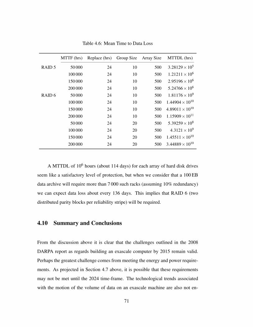
Table 4.6: Mean Time to Data Loss

MTTF (hrs) Replace (hrs) Group Size Array Size MTTDL (hrs)

RAID 5 50 000 24 10 500 3.28129×105

100 000 24 10 500 1.21211×106

150 000 24 10 500 2.95196×106

200 000 24 10 500 5.24766×106

RAID 6 50 000 24 10 500 1.81176×109

100 000 24 10 500 1.44904×1010

150 000 24 10 500 4.89011×1010

200 000 24 10 500 1.15909×1011

50 000 24 20 500 5.39259×108

100 000 24 20 500 4.3121×109

150 000 24 20 500 1.45511×1010

200 000 24 20 500 3.44889×1010

A MTTDL of 106 hours (about 114 days) for each array of hard disk drives

seem like a satisfactory level of protection, but when we consider that a 100 EB

data archive will require more than 7 000 such racks (assuming 10% redundancy)

we can expect data loss about every 136 days. This implies that RAID 6 (two

distributed parity blocks per reliability stripe) will be required.

4.10 Summary and Conclusions

From the discussion above it is clear that the challenges outlined in the 2008

DARPA report as regards building an exascale computer by 2015 remain valid.

Perhaps the greatest challenge comes from meeting the energy and power require-

ments. As projected in Section 4.7 above, it is possible that these requirements

may not be met until the 2024 time-frame. The technological trends associated

with the motion of the volume of data on an exascale machine are also not en-

71

couraging. Extrapolations of traditional processor technology and architecture

may simply make it impossible to achieve the very ambitious power and efficiency

goals. Memory and storage will also be limited for any future exascale system to

be contemplated for the 2020 time-frame. Memory density and bandwidth trends

are such that users of exascale systems will have to face challenges of limited

memory, and will not be able to scale the data volume for various applications;

bandwidth issues may result in inefficient utilization of the computational units of

future processors. Resilience remains an outstanding issue, and further research

is required to understand the implications. Finally, even archival storage looks

different at the exascale; it will be necessary to spin down almost all the drives

in the archival disk system in order to ensure that one does not exceed the power

budget of 20 MW.

Our findings regarding the issues examined in this section are as follows:

• It is likely that a platform that achieves an exaflop of peak performance

could be built in a 6–10 year time frame within the DOE/NNSA designated

power envelope of 20 megawatts. However, such a platform would have

limited memory capacity and memory bandwidth; owing to these limita-

tions such an exascale platform may not meet many DOE/NNSA applica-

tion requirements. We discuss this further in the next section where we

examine the requirements for a limited set of applications.

• The most serious technical challenge impeding the development of exascale

computing in the near term is the development of power-efficient architec-

tures that provide sufficient memory density and bandwidth for DOE/NNSA

applications. It is quite possible that meeting these challenges will require a

complete rethinking of processor architecture, at least for those portions of

the hardware that will be needed to address the DOE/NNSA workload.

72

5 REQUIREMENTS FOR DOE/NNSA APPLICA-TIONS

Having examined some of the hardware challenges associated with exascale com-

puting, we next examine some of the application requirements. We examine in this

section two applications that are of interest in light of the above discussion. The

first is climate modeling with the objective of resolving scales of motion that to

date cannot be accessed via present day capabilities. The second is high pressure

combustion with a similar objective, that is, attempting to include more physics at

scales that are typically modeled today.

To be sure, this selection of applications is highly idiosyncratic and basi-

cally reflects the authors’ fields of expertise. A more thorough study of this type

would include other important applications such as those occurring in materials

science, astrophysics, chemistry, biology, and other fields of inquiry where high

performance computing has played an important role.

5.1 Climate Simulation

We begin by considering an attractive target for exascale computing: the simula-

tion of atmospheric dynamics, particularly climate and weather, at a fine scale of

resolution. Accurate modeling of climate and weather is a pressing computational

challenge. To date, most of the assessment of climate and weather is performed

using a resolution of 200 km in longitude and latitude. The most ambitious such

simulations have resolved the earth at a scale of 25 km. To get a feel for how crude

this is, we show in Figure 5-1, in the first two images at left, the level at which

topography (expressed as surface altitude) is resolved at scales of 200 and 25 km

73

Figure 5-1: Surface altitude of the California coast shown at resolutions of 200km(left), 25 km (middle), and 1 km (right). From [51].

respectively. Modeling at this scale neglects or resolves poorly important moisture

transport processes associated with the dynamics of clouds, considered today one

of the key uncertainties in climate modeling. In fact, a significant portion of the

uncertainty in both short term (weather) and long term (climate) prediction is as-

sociated with the need to adequately represent moisture transport and in particular

formation of cloud cover.

Wehner et al. [51] have considered the requirements for running climate and

weather simulations that are resolved down to 1 km. This resolution is depicted

as the right-most image in Figure 5-1. At such a resolution, important features

such as orography become very clear. Their study does not consider the needed

improvements in the modeling of cloud physics that must be included in any sim-

ulation at this scale. But it examines requirements for simulating the climate and

weather using an existing and established modeling system: the Community At-

mospheric Model (CAM) developed at the National Center for Atmospheric Re-

search (NCAR).

74

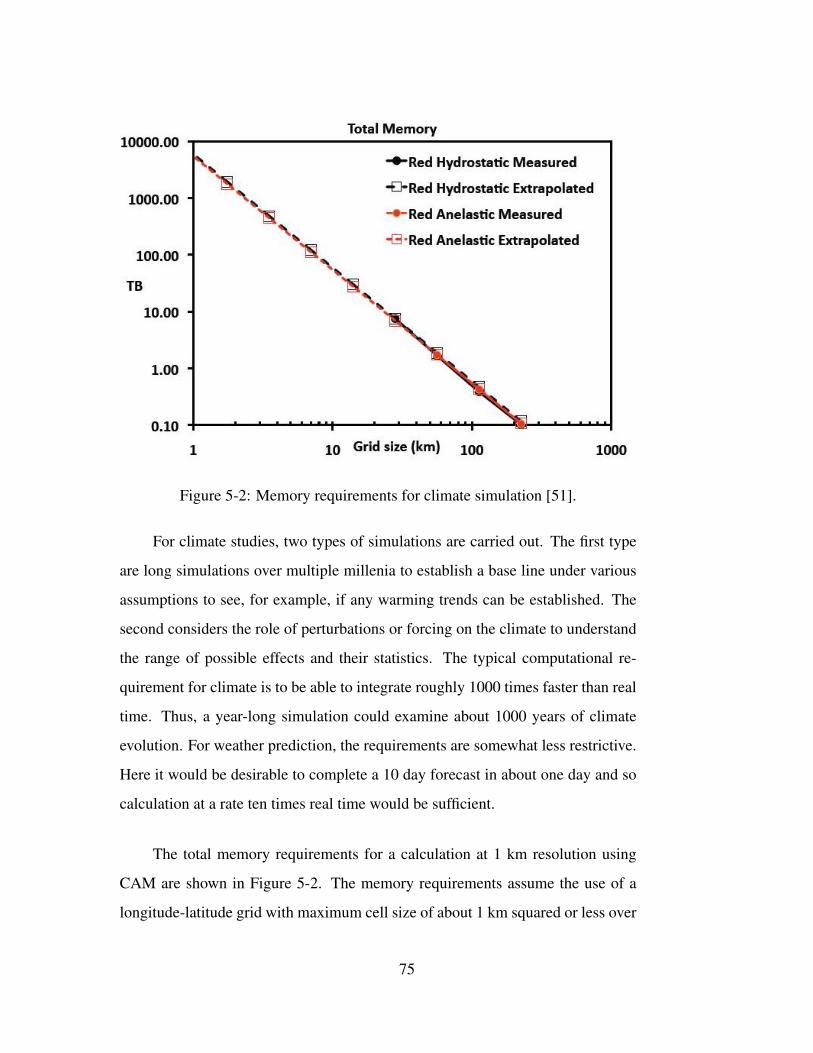
Figure 5-2: Memory requirements for climate simulation [51].

For climate studies, two types of simulations are carried out. The first type

are long simulations over multiple millenia to establish a base line under various

assumptions to see, for example, if any warming trends can be established. The

second considers the role of perturbations or forcing on the climate to understand

the range of possible effects and their statistics. The typical computational re-

quirement for climate is to be able to integrate roughly 1000 times faster than real

time. Thus, a year-long simulation could examine about 1000 years of climate

evolution. For weather prediction, the requirements are somewhat less restrictive.

Here it would be desirable to complete a 10 day forecast in about one day and so

calculation at a rate ten times real time would be sufficient.

The total memory requirements for a calculation at 1 km resolution using

CAM are shown in Figure 5-2. The memory requirements assume the use of a

longitude-latitude grid with maximum cell size of about 1 km squared or less over

75

the whole earth. The calculation is performed using a quasi-two-dimensional ap-

proximation of the three dimensional equations of motion with a vertical grid of

100 levels to capture vertical dynamics originating from the surface of the earth to

the edge of the atmosphere. The desired resolution is relatively insensitive to the

way in which the vertical direction is handled in such calculations, and the trends

for several approaches are shown in the Figure. In order to perform simulations

at a resolution of 1 km, roughly ten petabytes are required. This is well within

projections for the amount of provisioned memory on an exascale platform. The

relatively modest memory requirements result from the fact that the computation

is quasi-two-dimensional. It should be noted that this model still neglects impor-

tant physical phenomena and so even here a 1 km simulation would not constitute

direct numerical simulation of the earth’s climate. Modeling of various sub-scale

phenomena remains an important component of such simulations, but the ability

to resolve at scales on the order of 1 km is a useful investigation into the limita-

tions of the current models.

The requirements for exascale computation originate from the need to com-

pute at a rate of 1000 times faster than real time. These are shown in Figure 5-3.

It can be seen that different modeling approaches imply different floating point

requirements. The requirements for several approaches along with measurements

for those resolutions that are typically used today are shown in the Figure. Extrap-

olations of the results indicate that a sustained floating point throughput of 10 to

100 petaflops will be required to integrate the equations for a climate prediction at

a resolution of 1 km. For weather prediction, the requirements are 100 times less

severe as indicated previously. Because the typical percentage of peak floating

point performance realized with today’s modern processors is only typically 5%,

the peak required performance for this type of calculation is at least an exaflop.

76

Figure 5-3: Computational requirements for various climate modes [51]

This calculation could be performed if one scales present day architecture to

the exascale level but the energy costs would be prohibitive. Wehner et al [51]

examine the costs and indicate that 180 MW would be required to perform such

a computation using high power CMOS processors like those manufactured by

AMD or Intel. In contrast, 27 MW would be required for an extrapolation using

low power processors such as those introduced in IBM’s BG/L computer. Wehner

et al also examined the use of very low power processors such as those used in

today’s mobile devices. We will discuss the results of this study in Section 6.4

later on this report.

The overall conclusion however is that if sufficient progress is made in re-

ducing the energy costs of computing, it will be possible to perform some calcula-

tions of interest that exhibit low byte to flop memory bandwidth and total memory

requirements on exascale platforms perhaps as early as the 2020 time-frame.

77

5.2 Combustion

An important class of HPC applications involves fluid flow, or dynamics of mat-

ter, in general, where imposed stress fields and other boundary/energy dynam-

ics fluidize the material of interest. In this case, the unsteady three dimensional

flow velocity field, u(x, t) can be specified at each location, x, and time t. In

this approximation, the dynamical role of molecular collisions is well represented

by molecular-transport processes leading to momentum, temperature, and species

diffusion. The latter can be represented by the coefficients of viscosity, µ , heat

conductivity, k, and the i’th species diffusivity, Di respectively. These are ther-

modynamic functions of p and T only, and not flow-dependent. The resulting

abstraction is captured by the Navier-Stokes equations for continuum flow. While

even with that abstraction one can be led to challenging problems, the attendant

reduction in model dimensionality brings such flow problems within the realm of

computable physics on HPC platforms, as discussed below.

A very wide class of fluid-dynamics problems is addressable by the con-

tinuum approximation and the (implicit) local thermodynamic equilibrium (LTE)

assumption on which the attendant constitutive relations for molecular-transport

stresses and fluxes rely. Flow regimes for which this is not the case must resort to

more detailed descriptions. Even then, however, it is useful to ascertain that errors

made by the simpler continuum approximation, whose validity is (empirically)

found to extend beyond the regime where it would appear justified by a priori

considerations, exceed the inevitable errors in both statistics and representation in

the computation of solutions of the Boltzmann equation by Monte Carlo methods

or other means, and the associated collision integrals. The latter quickly become

intractable at higher fluid densities as the liquid phase is approached, whereas

the continuum approximation becomes ever better as fluid density increases. The

78

level of computational effort in solving for three-dimensional unsteady flow can

be estimated a priori by estimating the modal degrees of freedom of the problem.

For the purposes of illustration, we will limit the discussion to incompress-

ible flow, i.e., flow for which the local rms velocity, u′, is small compared to the

local speed of sound, a. More precisely, in terms of the appropriate dimension-

less parameter, we’ll consider flow at a small turbulence Mach number, i.e., small

M = u′/a. Fractional density variations scale as

∆ρ

ρ≈ M′2,

∆ρ

ρ< 0.05.

Since this scales local velocity fluctuations, this flow approximation can be as-

sumed valid if shock waves that may arise in supersonic flow, for example, are

handled explicitly as dividing dynamic surfaces between almost-incompressible-

flow regions. For three-dimensional fluid dynamics, the modal dimensionality can

be estimated as

Nmod ≈ αL∆x

3,

where L is the outer scale, e.g., L = 6m for a room-sized domain, ∆x is the small-

est spatial scale in the numerical simulation (grid size), and α is a proportionality

constant that depends on the type of discretization of the partial differential equa-

tions. The spatial grid size, ∆x, can be no larger than λmin/2, where λmin is the

smallest dynamical scale in the flow (per Nyquist). In terms of the smallest phys-

ical scale λmin, we must then have

Nmod ≈ 8α

(L

λmin

)3

.

For unsteady flow, the computational effort is also scaled by considerations

of time stepping in the numerics. For flow with a characteristic flow speed U , the

characteristic outer-flow time is given by τL = L/U and a simulation that captures

the statistical behavior of such a flow must simulate it for a total time that is at

79

least a few times τL. For an Eulerian simulation for which the coordinate system

is fixed, the simulation time step, ∆t, must be smaller than ∆x/U , with a number

of time steps per outer-flow time given by

Nt ≈LU

U∆x

=L∆x

.

Hence, the direct numerical simulation (DNS) computational effort (e.g., time

required for an exact solution of the partial differential equations of motion) is

proportional to

TDNS = Nmod ×Nt ≈ A(

L∆x

)4

.

where A is the computational effort per grid point/cell (e.g., the super-set of

floating-point operations, memory cycles, data communication time, or, in terms

of λmin

TDNS ≈ 16A(

Lλmin

)4

.

Two conclusions immediately follow. For a given computational effort per

grid point/cell, a doubling of the simulation spatial resolution, i.e., for λmin →

λmin/2, increases the computation effort by a factor of 24 = 16. Generally, if HPC

resources of a certain capability allow a resolution of the flow to a scale λ1, and a

higher resolution to a smaller scale λ2 < λ1 is required, the increase in the required

computation effort is given by (λ1/λ2)4. By way of example, if with a one petaflop

HPC resource one can correctly resolve flow down to spatial scales of say, λ1 =

1mm, and a higher resolution to λ2 = 0.01mm = 10µ is desired using the same

computational approach, computational resources are required with a capability

that scales across the board (all computational components) that is higher by a

factor of 104. That is, this requires a 10 exaflop capability.

Is the need for such spatial resolutions warranted? For the simplest turbu-

lent flows, the appropriate dimensionless flow-scaling parameter is the Reynolds

80

number,

Re =ρUL

µ=

ULν

,

where ν = µ/ρ is the ratio of the dynamic (shear) viscosity to the fluid density,

with units of area per unit time (ν = 0.15cm2/s for air at normal T and p). In terms

of Re, the smallest fluid-dynamical physical scale is given by the Kolmogorov

scale, which can be expressed as a fraction of the outer scale L, i.e.,

λK

L= CKRe−3/4,

with a constant of proportionality, CK , of order unity. Again by way of example,

if a d0 = 1m diameter duct is discharging air into a room at a speed of U = 10

m/s, the relevant Reynolds number would be given by Re = d0U/ν ≈ 6.7×105,

yielding a Kolmogorov scale λK/d0 ≈ Re−3/4 ≈ 4.3× 10−5, corresponding to a

dynamic range of L/λmin ≈ 2.3×104, or λmin ≈ 43µ in dimensional units, for this

quite modest flow. Higher speeds would lead to smaller minimum physical scales

yet. Scaling the computational effort in terms of Re and identifying λmin with λK ,

we also see that

EDNS ≈ 16ARe3.

Bona fide turbulence requires minimum Reynolds numbers in the range of Remin ≈

1−2×104, with values for real/practical turbulent flows of order Re = 105−106

and higher frequently encountered, so micron-size minimum spatial scales are not

uncommon in high Reynolds number turbulence.

At this writing, spatial dynamic-ranges attained in direct fluid-dynamic sim-

ulations (DNS) on HPC platforms in idealized-flow situations and boundary con-

ditions are of order L/λmin ≈ 4000. Flows with realistic boundary conditions

that must deal with modest multi-physics elements have reached a dynamic range

about half that, or L/λmin ≈ 2000, i.e., about an order of magnitude lower than the

simple duct-discharge flow in the example above. A brute-force DNS approach

81

would then require a HPC capability of order 104 times higher than provided by

today’s HPC resources. We conclude that even the level of simplification afforded

by the continuum approximation, a wide class of representative fluid-dynamics

problems is not within reach of numerical solutions by direct (DNS) methods,

even with exascale HPC resources. The fourth-power cost of successive dou-

blings in resolution improvement indicates that computing power, alone, does not

offer a promising path. Typical fluid dynamics problems that are coupled with

multi-physics phenomena, such as radiation, inhomogeneous density fields and

compressibility, chemically reacting flows with local heat release, are even fur-

ther beyond reach.

Is there, or are there, alternative paths? Is it necessary to resolve the smallest

fluid-dynamic scales in all cases? Is it sometimes adequate to model their con-

tribution to the dynamics in some manner? The answer in many cases depends

on the question(s) asked. The spectrum of turbulence is such that kinetic energy

associated with a particular scale rapidly decreases with decreasing scale size.

Capturing, say, 80% of the kinetic energy, or more, can typically be achieved by

capturing a large-to-small scale dynamic range 2.5 to 3 orders of magnitude, i.e.,

the ratio of the lowest (kmin ≈ 1/L) to the highest (kmax ≈ 1/∆x) wavenumbers

resolved. Such simulations are called large-eddy simulation (LES) calculations.

Significantly, such a dynamic range can be hosted on petascale HPC resources.

Predictive LES calculations rely on explicit or implicit models that capture the

contribution of unresolved scales to the overall dynamics, called subgrid-scale

(SGS) models. At this writing, SGS models exist that are fluid-dynamically cor-

rect for (near-) uniform-density flows, but none exist for non-uniform-density

flows, to our knowledge. If the questions rely on processes that predominantly

occur at the smallest scales, the onus on correct SGS modeling is greater. Mixing

that takes place at (molecular) diffusion scales provides an example, especially as

82

a precursor to chemical reactions, as discussed below. Its correct quantification is

essential in combustion. Advances in modeling SGS dynamics to non-uniform-

density flows would place a large swath of fluid dynamics within reach of HPC re-

sources. Such LES-SGS modeling can then provide the backbone to host a variety

of multi-physics phenomena coupled to fluid dynamics. As the discussion above

suggests, however, absent such progress, increasing HPC capability alone will

not get us there. Before ending this section, we note that details of the numerics

used to solve the system of partial-differential equations (PDEs) that describe the

flow are also important. Representations of derivatives, for example, can lead to

numerical dissipation that is, dynamically, indistinguishable from physical fluid-

dynamic dissipation (viscous effects, mixing and diffusion, heat conduction, etc.)

in the simulation. Such effects can mask the intentional representation of SGS

dynamics included in the LES-SGS framework and, even with physically correct

SGS models intentionally incorporated, the simulations can be incorrect.

Chemically reacting flows and combustion, pose two different challenges. If

the flow hosting the combustion is itself turbulent, its analysis must address and

respond to all the challenges described above. In addition, the complexity of de-

tailed chemical kinetics simulations, the effect of heat release at small scales of

the flow, and the change in the flow environment that, in turn, dictates the combus-

tion environment must be addressed. To help assess and scale the challenge, we

note that simulating fluid dynamics requires the solution of two scalar equations

(for conservation of mass and energy) and one vector equation (for conservation

of momentum), for a total of five scalar equations, constrained by an equation of

state for the fluid and augmented by constitutive relations for molecular stresses

and fluxes. If fluid species react, a species-transport/-conservation equation must

be included for each one, with a diffusive term that can itself be quite complex;

diffusion of a particular species in a mixture depends on the surrounding molec-

83

ular environment; a process termed multi-component diffusion. Further, detailed

chemical kinetics of the combustion of a hydrocarbon fuel, such as diesel, are

expressed in terms of hundreds of chemical species and hundreds to thousands

of elementary reactions. Given K species, one can expect that the number of

elementary reactions would increase combinatorially with K, since all possible

combinations of reactants can, in principle, participate in such reactions. Detailed

chemical-kinetic models of combustion for higher-hydrocarbon fuels, however,

typically entail a number of reactions that is a multiple of K, on average, about 100

elementary reactions per species. No fundamental theory or methodology exists

today to estimate the elementary reactions that participate, or that are important

and must be included in a detailed chemical-kinetic model. That aside, with four

constants typically needed to describe the Arrhenius form of reaction rates, such

models rely on thousands of constants that are, for the most part, poorly known.

It helps to classify combustion into modes. An important classification con-

siders whether the fuel and oxidizer are either perfectly mixed or perfectly un-

mixed before chemical reactions occur. In the former, we speak of premixed

combustion while in the latter we speak of non-premixed combustion. However,

depending on the relative magnitude of the mixing-diffusion flow time, τ f , and

the chemical-kinetic time, τξ , combustion will proceed in an environment that is

in an intermediate regime, i.e., in neither limit. The ratio of these two times is

called the Damkohler number,

Da ≡τ f

τξ

.

Combustion will occur in thin sheets, or flamelets, for high values of Da, or in

distributed regions for low values of Da. Further, one can be in a high-Da regime

for some elementary reactions and a low-Da regime for others, while all reac-

tions participate in the combustion process. Unreacted mixtures can ignite and

burn by their own means (autoignition, at high temperatures, for example) or by

84

an external heat/energy source (ignition). In the second case, called a premixed

flame, a thin reactive zone can advance into a region of unreacted species as a

wave. For typical hydrocarbon combustion, density decreases by a factor of about

7 across such a flame. Matters are further complicated because, depending on

the fluid-dynamic environment, a burning region can be locally extinguished and

then reignite, leading to a combustion environment that strongly depends on the

Lagrangian history of a fluid/reactant parcel as well as its environment, and is not

local in space-time.

To summarize this discussion, the number of PDEs that must be solved for

turbulent combustion is one to two orders of magnitude larger than for fluid dy-

namics alone. The computational effort is typically quite a bit larger as transport

equations now have to be solved for each species. Time-stepping becomes very

stiff because of the large range in chemical-reaction times, and the spatial res-

olution required for thin flames can be locally high. As a result, strict DNS of

turbulent combustion of hydrocarbons will likely remain beyond reach, even with

exascale HPC resources.

A few additional challenges are worth listing. With unknown detailed chemi-

cal-kinetic models, at least for higher-hydrocarbon fuels, the equations that must

be solved are not known. If the challenge in predicting higher-hydrocarbon com-

bustion is the chemical-kinetic models, it would appear prudent to attempt the

simulation in a well-controlled environment that can be diagnosed to the requisite

precision and accuracy, so comparisons with numerical predictions can be made.

Turbulence with its own challenges, as discussed above, does not appear to offer

the most convenient or promising environment. While a set of elementary reac-

tions may offer a complete description, at least over a range of conditions, which

of those reactions dominate will depend on the combustion environment. By way

85

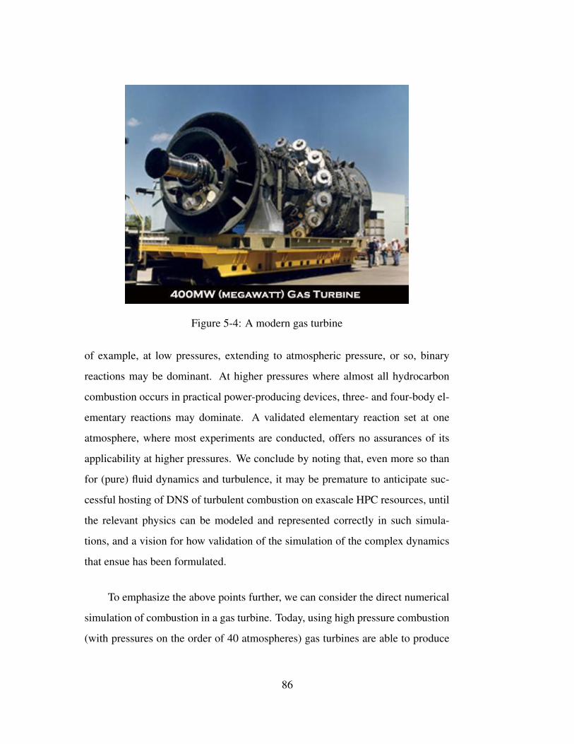
Figure 5-4: A modern gas turbine

of example, at low pressures, extending to atmospheric pressure, or so, binary

reactions may be dominant. At higher pressures where almost all hydrocarbon

combustion occurs in practical power-producing devices, three- and four-body el-

ementary reactions may dominate. A validated elementary reaction set at one

atmosphere, where most experiments are conducted, offers no assurances of its

applicability at higher pressures. We conclude by noting that, even more so than

for (pure) fluid dynamics and turbulence, it may be premature to anticipate suc-

cessful hosting of DNS of turbulent combustion on exascale HPC resources, until

the relevant physics can be modeled and represented correctly in such simula-

tions, and a vision for how validation of the simulation of the complex dynamics

that ensue has been formulated.

To emphasize the above points further, we can consider the direct numerical

simulation of combustion in a gas turbine. Today, using high pressure combustion

(with pressures on the order of 40 atmospheres) gas turbines are able to produce

86

significant power outputs. The scale of such turbines is quite large as shown in

Figure 5-4; The turbine shown in the figure is able to output 400 MW of power.

In the combustion chamber of the turbine, the Reynolds number Re can reach

values on the order of 106 – 107 which indicates a strongly turbulent flow. A

direct numerical simulation of a flow such as this down to the Kolmogorov scale

will require the ability to resolve a length scale 105 smaller than the characteristic

length of the combustor.

The computational requirements for such a calculation given the considera-

tions above are daunting. It is necessary to track the density, the three velocity

components, and the energy of the fluid to resolve only the fluid mechanics of the

combustion process. In order only to resolve the flow we require 1015 cells per

field. Temporary fields must also be maintained for time integration as well as

the computation of the various terms in the Navier-Stokes equations. The number

of such fields will depend on the particular advection algorithm employed, but it

is conceivable that one would require on the order of 150 petabytes of memory

for the fluid mechanics alone. For a proposed exascale platform with a memory

of say 50 petabytes (considered a typical target) this calculation cannot be done.

Simulation of problems at these Reynolds numbers will still require turbulence

modeling.

We have not yet considered the requirements for simulation of the chemistry.

This proceeds through the integration of chemical rate equations which describe

the various reactions that take place as the combustion proceeds. As discussed

above, for complex hydrocarbons, a large number of species must be tracked and

so the requirements for storage of the chemical species alone will greatly exceed

the number of fields required to store the fields used to describe conservation of

mass, momentum and energy. The memory requirements for such a calculation

87

Figure 5-5: Projected performance of NNSA applications using extrapolations ofcurrent hardware capabilities. The vertical axis is in petaflops. The top dashedline represents requirements as projected by NNSA for predictive capability forkey phenomena associated with stockpile stewardship. The blue curve indicatesprojects peak capability. The red region derates this due to memory limitations.The green curve further derates this performance based on memory bandwidthprojections [46].

are now well into the exabyte range.

The implications of the discussion above is that some calculations of inter-

est to the DOE/NNSA mission will not be achievable without a larger memory

capacity than is currently envisaged, These considerations do not even take into

account memory bandwidth issues and energy costs.

88

5.3 NNSA Applications

We discuss here very briefly the application requirements for NNSA applications

used as part of the stockpile stewardship mission. The nature of the codes and

the specific applications are discussed in a classified appendix to this report (Ap-

pendix C).

NNSA applications are more complex in terms of the simulated physics than

the combustion applications discussed above. As discussed in Appendix C, to

achieve DOE/NNSA mission needs, continued advances in computing capability

to the exascale level and likely beyond are required and will be required for the

foreseeable future. However, as also discussed in the classified appendix, ow-

ing to the integrated way in which the stewardship mission is carried out with a

reliance on test data, experiment and computation, there is no particular thresh-

old requirement for exascale capability in the 2020 time frame as regards those

national security issues associated with the DOE/NNSA mission.

Various aspects of the performance of NNSA stewardship applications have

been examined in detail. Figure 5-5 shows the evolution of peak performance over

time. The dashed curve at the top of the figure indicates desired progress for exas-

cale capability by 2020. The solid blue curve indicates projected peak capability.

This is displayed as a range depending on the nature of the application. How-

ever, at present because NNSA stewardship applications require a large amount of

memory per thread of execution, memory capacity limitations will make it impos-

sible to expose the required level of parallelism without significant restructuring of

the algorithms. This is represented by the red set of curves again showing a range

of throughputs. Finally, the stewardship applications require at present significant

memory bandwidth. Using projections for future hardware this derates perfor-

89

mance further and is shown as the set of green curves. The implication is that an

exascale platform will perform at low efficiency for stewardship applications with

a sustained performance no better than several petaflops unless improvements are

made in future architectures to address these issues.

5.4 Summary and Conclusion

Our findings as regards application requirements above are as follows:

• It is likely that a platform that achieves an exaflop of peak performance

could be built in a 6–10 year time frame within the DOE/NNSA designated

power envelope of 20 MW. However, such a platform would have limited

memory capacity and memory bandwidth; owing to these limitations such

an exascale platform may not meet many DOE/NNSA application require-

ments. This finding is repeated from Section 4.10. It will be possible to

accomplish some important computations relevant to the DOE mission but,

as exemplified in the section on combustion, there will also be a class of sci-

entifically compelling calculations that will require more memory capacity

and bandwidth.

• To achieve DOE/NNSA mission needs, continued advances in computing

capability are required and will be required for the foreseeable future. How-

ever, there is no particular threshold requirement for exascale capability in

the 2020 time frame as regards those national security issues associated with

the DOE/NNSA mission. For this reason, JASON does not foresee signifi-

cant national security impacts associated with a failure to execute the DOE

Exascale Computing Initiative by 2020.

• To date, our understanding of the computational requirements for DOE/-

90

NNSA applications, particularly issues of memory bandwidth and floating

point throughput, remain murky. At present it is simply not possible to

know how DOE/NNSA applications will perform on proposed future archi-

tectures. More focus is required to ensure that the hardware and software

under development in support of an exascale capability will address per-

formance improvements specific to the communication and computational

patterns of DOE/NNSA applications. A coordinated DOE/NNSA effort is

required to characterize in a standard way the computational patterns and

characteristics (i.e. memory capacity, memory bandwidth, floating point in-

tensity and global communication ) of the suite of DOE/NNSA applications.

Only in this way will it be possible to understand if traditional extensions

of modern microprocessor architecture will make it possible to achieve bal-

anced exascale performance or whether a completely different approach is

required.

91

6 RESEARCH DIRECTIONS

In this section we examine several promising hardware research directions to ad-

dress some of the hardware challenges discussed previously.

6.1 Breaking the Memory Wall

As has been noted previously, memory bandwidth performance has not kept pace

with the increase in speed of modern microprocessors. There are several issues

here such as the energy cost of data transport and the fact that DRAM memories

are designed for memory density as opposed to low data access latency.

A recent development in memory technology has been the introduction of

through-silicon-via (TSV) memories. These memories can be stacked on each

other to build a dense memory system and on a processor chip to increase inter-

connect bandwidth and decrease off-chip communication energy. An example of

TSV silicon technology is shown in Figure 6-1.

The JEDEC “wide-IO” memory standard aimed at mobile devices, in partic-

ular, cell phones and tablets, is the first of these TSV memories. The JEDEC

“high-bandwidth memory” (HBM) (also called graphics wide-IO) is a higher-

bandwidth version expected out in a few years. TSV memories have very wide

interfaces (up to 1K bits for the JEDEC HBM) and essentially eliminate the off-

chip component of energy. These can be stacked on a processor die, but may be

more practical stacked next to the die on a silicon “interposer”. Only a few chips

– at most 16-32 can be packaged with one processor die, so only a limited ca-

pacity (about 16 GB) of high-bandwidth (low energy per bit) DRAM is available

on a processor node. To build a large memory system, one needs to either build

93

Figure 6-1: Silicon layers arrayed vertically to create higher density memories

many very small nodes (6.4 M for 100PB) or have an additional level of hierar-

chy. Because TSV memories (even the standard ones) carry a cost premium, it is

expected that an exascale system will use commodity memory for its main mem-

ory and TSV memory for a level of hierarchy just below main memory. Such a

memory could serve as a 16 GB last-level cache.

JASON was briefed on similar TSV technology from Micron. Micron’s hy-

brid memory cube (HMC) is a TSV memory (like HBM) stacked on a proprietary

logic layer with a proprietary signaling interface back to the processor. Like any

HPC memory technology, HMC needs to be judged on two simple metrics, cost

per bit and energy per bit, and compared not against today’s DRAM memory tech-

nology (DDR3), but against expected commodity DRAM that is expected to be

$1.25-2.50/GB and have an access energy of 5-10 pJ/bit. Exploiting functions in

the logic layer presents interesting possibilities, but that is basically the equivalent

of building many small processors with attached TSV memory (the 6.4 M proces-

sors with 16 GB each vs. 200K processors with 512 GB each) and will create yet

94

Figure 6-2: The Micron memory cube

another layer of complexity for programmers. Both the JEDEC HBM and Micron

technologies are promising and should be explored in future architectures.

There have been many proposed technologies for DRAM replacements in-

cluding phase change memories, memristors, spin-torque memories, etc. To the

extent that these can be fabricated with a cost per bit less than DRAM, they may

affect the capacity part of the memory problem. However, to a first approximation

they will not improve the memory bandwidth because memory bandwidth is lim-

ited by energy and that energy is dominated by on- and off-chip communication,

not by the actual memory cell or sub-array.

There have been proposals to connect to DRAM with integrated optics. The

success of this approach again depends on communication energy. While there

are many promising optical developments, no real demonstrated system has come

close to the 1-2 pJ/bit demonstrated for electrical signaling at these rates and dis-

tances. The best demonstrated optical channels today consume upwards of 20 pJ

per bit when all factors (not just the modulator and receiver) are considered. Op-

tical technologies are discussed further below.

95

Figure 6-3: A sample of various photonic devices

To sum up, memory capacity is a question of cost and memory bandwidth

and is constrained by on- and off-chip signaling energy. Commodity memory is

likely to get to $1.25 to $2.50/GB by 2020 and 5–10 pJ/bit. If TSV memories can

achieve comparable cost (they are currently two times to four times SDDR costs)

they can eliminate most of the off-chip communication energy driving total access

energy to the 1–3 pJ/bit range. However, only a relatively small amount of TSV

memory (16 GB) can be packaged near any one processor presenting challenges in

overall system organization and scaling so issues of memory capacity will remain.

6.2 Role of Photonics for Exascale Computing

Performance scalability of computing systems has been and will continue to be

increasingly constrained by both the power required and speed available to en-

able data communications between memory and processor as discussed above.

Optical links, with the capability for high-bandwidth information transfer (wave-

length domain parallelism), and low transmission energy dissipation have long

held promise for off-chip communications, and may play an increasingly criti-

96

cal role in linking processors on a common circuit card. The idea generally is

that electrical signals modulate optical signals which can be efficiently routed via

optical waveguides or through fibers. Indeed, optical interconnects have already

been employed in high performance computers: the IBM Roadrunner has used

short-reach active optical cables (AOCs) based on vertical-cavity surface-emitting

lasers and multimode fibers (VCSEL/MMs). These VCSEL transceivers provide

over 100,000 optical ports per system and facilitate the achievement of high ag-

gregate bandwidth communications between racks and the central switch [15].

Extensions to exascale computing will necessitate more comprehensive intercom-

munications (racks, boards, modules, chips), a massive increase in the number of

parallel optical links (≈ 100 million) with high reliability, low power dissipation

and low cost. Recently, a 25 Gb/s, 6.5 pJ/bit optical link was reported, utilizing

10 Gb/s class VCSELs, with electronics built into a 90 nm CMOS process [40].

These researchers anticipate building on future developments in faster VCSELs,

mandated by industry-wide development for 100 Gb Ethernet applications. The

feasibility of on-chip photonic integration has been driven by advances in ma-

terials and device design that allowed the scaling of typical optical components

(waveguides, modulators, receivers, detectors, couplers and switches) with low

loss. Some of these concepts are shown in Figure 6-3. Typical silicon waveguide

cross-sectional areas are 0.1 micron2 and the bending radii of waveguides are as

small at 1 micron [35]. This scaling down in size of critical optical components

makes possible higher density integration of photonic switches, links and modu-

lators, but it is also subject to issues of crosstalk.

The trade-offs between bandwidth, power and cost will have to be fully eval-

uated. Total power dissipation will very much depend on device choices (e.g.,

ring micro-ring demultiplexers), choices of materials and the details of the sys-

tem architecture. Many of those decisions and implementations are still being

97

explored. Total sources of energy/information loss must also be fully understood

(for example insertion loss from fiber to chip, from modulator to modulator). In

addition, the power efficiency per device component (e.g. modulator) must be un-

derstood and accounted for. Finally, there may be some energy costs to stabilizing

the performance or tuning the response of optical components (e.g. [17]).

Ultimately, the choice of laser (optical source), its type (VCSEL1, DFB2), its

efficiency and the efficiency of coupling on-chip will be a large determinant of the

energy/bit for the optical links, and in the efforts to drive down the energy dissi-

pation to a few pJ/bit. Although detailed simulations have been done of insertion

loss, crosstalk and power requirements for simple chip-scale photonic intercon-

nects, it is not at all clear how well these simulations might describe the further

scale up of density and complexity that will be required to mediate the memory

wall for exascale computers [6]. In addition, there are a variety of 3D geometries

being considered for the integration of the photonic layer with the microproces-

sor layer. Thus, although photonic interconnects have already played an important

role in high performance computing, the short-term realization of a photonic tech-

nology that will address the memory wall challenge of exascale computing is not

clear. At the moment there are a variety of different device implementations being

pursued, different means of integration (e.g. hybrid via flip-chip or full integration

with CMOS), and challenges in understanding how to accurately assess energy ef-

ficiency, data-rate capabilities and other metrics of performance for truly scaled

photonic circuits.

98

6.3 Computation and Communication Patterns of DOE/NNSAApplications

It has been observed by Phil Colella [4] that the scientific applications of interest

to both NNSA and DOE possess common communication and computation pat-

terns. Colella noted there were seven such patterns and named them “the seven

dwarfs of high performance computing”. In Figure 6-4 these patterns are listed

and symbolized by their respective inter-processor communication patterns. The

greater the amount of data that must be transferred between processor i to proces-

sor j the brighter is the dot in the images. We discuss these dwarfs briefly:

Dense linear algebra This class of applications is characterized by operations on

dense matrices such as matrix-matrix multiplies. Such operations exhibit

high data locality and a very regular access pattern; with proper caching of

matrix elements a significant amount of data reuse can be achieved. For this

pattern a very high flop to byte ratio is achievable. Such applications (for

example the LINPACK benchmark) can be run very efficiently on modern

microprocessors. In Figure 6-4 we show the inter-processor communication

pattern for matrix-matrix multiply.

Sparse linear algebra This class of applications is characterized by operations

on sparse matrices. These can be very challenging to implement on paral-

lel architectures because the sparsity pattern makes it difficult to optimize

based on locality. Typically one must permute the matrix so that the el-

ements on a given row are mutually as close as possible to one another.

Finding such an optimal permutation is accomplished using graph-theoretic

approaches, but because these are themselves computationally complex, one

often resorts to heuristics based on the nature of the problem. In addition, it

is essential to store the sparse matrix in a compact format since most of the

99

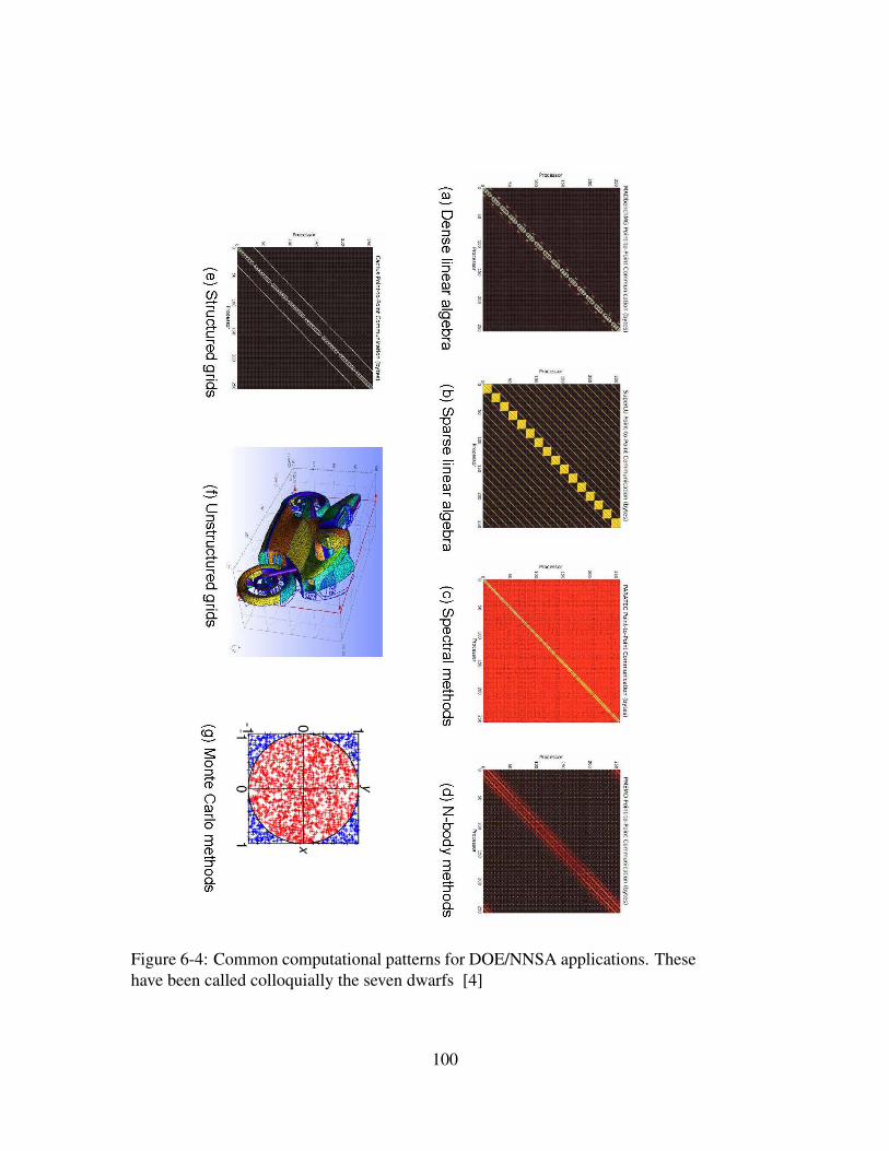
Figure 6-4: Common computational patterns for DOE/NNSA applications. Thesehave been called colloquially the seven dwarfs [4]

100

elements are zeroes.

Spectral methods Spectral methods utilize expansions in complete sets of func-

tions to represent solutions to various partial differential equations. The

dominant communication pattern is a general matrix multiply associated

with a transformation from physical space to some set of expansion coef-

ficients. If the expansion is in terms of trigonometric functions then fast

methods can be used in one or more coordinate directions. However, be-

cause the fields for a spectral method are typically rectangular arrays de-

composed across processors, it is often necessary to perform a transposition

of the array in order to perform transforms in all coordinate directions. As

a result, these methods require all-to-all communication of the entire array.

This is shown in Figure 6-4(c) where the all-to-all processor communication

pattern becomes readily apparent.

N-body methods These methods are used to compute interactions among a group

of particles interacting via some prescribed force law. Examples are grav-

itational dynamics or motion of charged particles. There exist optimized

approaches based on the idea of multipole expansions to efficiently evalu-

ate the relevant interactions. The typical data structures are tree-based and

use various labeling approaches such as space-filling curves to enhance data

locality. A typical communication pattern is shown in Figure 6-4(d).

Structured grids The discretization of a partial differential equation onto a reg-

ular rectangular grid or a set of rectangular grids using techniques such as

finite difference or finite element methods results in a sparse matrix with

very regular structure. Operations using such matrices are very efficient be-

cause the data pattern is highly regular provided one takes advantage of the

spatial locality of the data. A typical communication pattern is shown in

Figure 6-4(e).

101

Unstructured grids An example of this pattern is the use of finite element meth-

ods to discretize partial differential equations on complex geometries such

as the one shown in Figure 6-4(f). Graph-theoretic methods must again be

used to label the points of the unstructured mesh to ensure maximal data

locality and scatter-gather operations are then required to assemble the re-

sulting sparse matrices. The solution of the resulting equations can be ac-

complished using the approaches associated with the sparse linear algebra

dwarf, but typically, because the matrices involved come from a continuous

operator, iterative methods are employed and these too can be optimized so

that data locality is maximized.

Monte-Carlo methods These approaches are exemplified by the computation of

high dimensional integrals by means of summation over randomly selected

sets of points over a given domain. Operations are basically embarrassingly

parallel meaning evaluation of the integrands can proceed with little or no

communication among processors. However, collective operations are re-

quired to compute the expectation values over the probability distribution.

In Figure 6-4 we symbolize this approach through the use of the computa-

tion of the number π by choosing random points and seeing whether their

location is inside or outside a circle of radius 1.

If a specific dwarf is applicable to a given problem, it is possible to take ad-

vantage of the fact that the communication and computational patterns are well-

defined. In this case it is possible to improve performance via software optimiza-

tion or hardware optimization. The idea of classifying the communication and

computation patterns of a given application is not new. In some sense, object-

oriented computing was developed with this idea in mind for general purpose

programming, but the notion of the dwarf goes somewhat further in that one un-

derstands ahead of time the data flow and so can develop not only class libraries

102

but whole template codes for important operations. Chandy et al put forth a sim-

ilar idea in their discussion of programming “archetypes” [7]. We discuss opti-

mization approaches using hardware briefly below. Software optimizations are

discussed in Section 7.

6.4 Optimizing Hardware for Computational Patterns

One approach to optimizing performance is to develop special purpose hard-

ware for specific problems. This has been attempted several times for specific

applications. The most recent approach has been the development of a special

purpose machine for computation of protein folding by D. Shaw et al. [44]. Such

approaches have produced impressive results for specific target problems. How-

ever, since these architectures are not general purpose, they are not viewed as a

credible path to exascale computing.

We briefly describe an approach that is intermediate between general pur-

pose and special purpose computers. We were briefed by Michael Wehner [50]

on the Green Flash project at Berkeley. In this work the climate modeling appli-

cation discussed in Section 5.1 was used as a target application and a reference

hardware design was constructed. The climate simulation application uses the

structured grid dwarf and so it is possible to allocate processor resources such as

cache memory etc in such a way that while the hardware remains general purpose,

it is tuned so that optimal performance is obtained for this particular application

and by extension any application that fits the associated computational pattern.

Several hardware designs were considered including the use of standard high

103

Figure 6-5: Tensilica chip shown in apposition to several larger scale generalpurpose microprocessors [39]. Note only one core of a double precision Tensilicadesign is shown. A custom processor would be built from a collection of suchcores.

power CMOS chips such as the AMD Opteron and low power chips such as those

used in IBM’s BlueGene. The authors also examined the use of ultra low power

processors such as those being developed for the cell phone industry. These com-

panies develop custom processors based on the specifications provided by the

specific phone manufacturer with the advantage that the desired functionality (and

only that functionality) is provisioned onto the processor. Companies such as Ten-

silica provide prepackaged logic circuits (called IP cores) that provide the desired

functionality. The entire chip can be laid out and then simulated using special

software development environments on standard workstations. Once the desired

chip is in hand, it can be fabricated or translated into a specification for further

testing using field programmable gate arrays (FPGAs).

The design point for the climate application reached by Wehner et al. is in-

104

teresting because it takes advantage of the understanding of the relevant dwarf

and trades off individual processor power (of the type seen in typical general pur-

pose processors) for limited capability and massive parallelism. For example,

using 22 nm silicon, Wehner et al. [51] proposed a chip with 512 low power cores

clocked at only 650 MHz. In order to achieve the requirements for a 1–2 km res-

olution climate simulation each core would have to produce 1.3 GFlops on the

target application. They also determined that a cache size of 256 kB per core

would be sufficient to mask memory latency.

The cores utilized for this exercise are very small relative to modern general

purpose processors. The relative size is shown in Figure 6-5. There are also

advantages in terms of power utilization. For example an IBM Power 5 processor

clocked at 1.9GHz dissipates 120W. In contrast 128 Tensilica cores of the type

considered by Wehner et al dissipate a total of only 11.5W .

We do not advocate that special purpose machines be built for DOE/NNSA

applications. However, given that a significant portion of these applications can

be classified by a dwarf (or some composition of dwarfs), a limited hardware ex-

ploration effort to design hardware accelerators for dwarfs (either on-processor or

off-processor) that support a specific computational pattern may be useful. Such

an effort would make it possible to compare the performance of more general pur-

pose hardware solutions, and this in turn would make it possible to make more

informed decisions as regards the potential for performance of DOE/NNSA ap-

plications. We believe there is a role for a limited hardware development effort to

encourage potential advances that then could be migrated into vendor hardware.

105

7 SOFTWARE CHALLENGES

In this section, we describe some promising research directions for the develop-

ment of exascale software. As HPC architectures become more heterogeneous

and hierarchical, the challenges of modifying science application codes to utilize

them effectively sometimes rival in magnitude the challenges faced in developing

the hardware platform. While the ASC program was largely successful in porting

key science applications to the very heterogeneous Roadrunner for example, it is

widely held that much of the porting work involved “heroic” efforts.

At present the dominant approach for programming massively parallel sys-

tems is the Message Passing Interface (MPI). In MPI, the programmer is respon-

sible for managing all interprocess communication. MPI has been successful be-

cause it is a standard supported on all platforms and, in many cases, vendors have

provided special libraries that facilitate optimized data transfer using hardware

features specific to the particular architecture. In addition, MPI allows one to rea-

son about a computation in a way that is independent of particular node or network

configurations by using the concept of the “communicator,” a virtual context for

parallel communication. For heterogeneous architectures, MPI has been used in

combination with compiler directives and libraries (such as OpenMP) so that effi-

cient thread-based parallelism can be employed on multicore architectures while

interprocessor communication is performed using traditional MPI. Recently, there

has also been important work on using MPI with GPU architecture, allowing for

direct access to GPU memories so that data can be moved in a way that is more

uniform and transparent to the programmer [1].

We expect that the MPI approach will remain an important aspect of parallel

programming. However, it is anticipated that the need to manage a billion threads

107

creates a level of complexity which may make the direct use of MPI untenable.

Instead, there will be a need to hide many of the implementation details from the

programmer. It is also the case that optimizing performance for an exascale sys-

tem may also require automated approaches. The need to provide software that

facilitates programmer productivity is known to be a challenging issue. We dis-

cuss two ideas which we feel have merit and deserve further exploration. The first

is the use of domain-specific languages wherein one constructs simple languages

that embody a specific computation and communication pattern. The second is

the use of autotuning software to optimize system and program parameters so that

maximal hardware throughput is enabled. These approaches can potentially alle-

viate some of the burden of porting applications to new architectures, and could

greatly improve the productivity of the science programmer, especially during the

key phases when new architectures are introduced.

7.1 Domain Specific Compilers and Languages

A domain-specific compiler is a special type of compiler that uses knowledge of

the computational problem domain to build more efficient code than can be pro-

duced using a general-purpose compiler. Domain-specific languages (DSLs) take

domain-specific compilers one step further, and are typically designed to allow

the programmer to describe the computational algorithm at a very high level that

is usually independent of the underlying architecture. To allow the application

programmer to “speak” at such a high level of course requires that knowledge

of the target hardware platform is encoded in the compiler so that it can gen-

erate usable code. While this requires significant effort in practice, the payoff

is that when the application must be ported to a new architecture, modifications

only need to be made to the compiler. This separation of the problem descrip-

108

var i = 0;

while ( i < 1000 ) {

Flux(vertices(mesh))= 0.f;

JacobiStep(vertices(mesh)) = 0.f;

for (e <- edges(mesh)) {

val v1 = head(e);

val v2 = tail(e);

val dP = Position(v1) - Position(v2);

val dT = Temperature(v1) - Temperature(v2);

val step = 1.0f/(length(dP));

Flux(v1) += dT*step;

Flux(v2) -= dT*step;

JacobiStep(v1) += step;

JacobiStep(v2) += step }

i += 1 }

}

Figure 7-1: Example Liszt code that performs heat conduction on a grid.

tion and the hardware implementation is especially useful given the way in which

DOE/NNSA application codes are used at the respective laboratories—namely,

the physics in the codes is continually being modified in response to research

needs. Having to maintain both the evolving physics components of these large

codes and the corresponding hardware-specific implementation requires physi-

cists with computer scientist-level programming ability, and computer scientists

with PhD-level physics knowledge. Although such remarkable people exist at the

labs, it is very natural and feasible (though admittedly difficult) to separate the

domain-specific problem description from the hardware-specific implementation.

Although domain-specific languages find common use in the software engi-

neering world (e.g., the ColdFusion Markup Language for rapid website devel-

opment), their use in the scientific world appears rare. One particularly com-

pelling DSL for scientific applications (and one that was briefed to us) is the

Liszt language for solving mesh-based PDEs [19]. Liszt is a mature language

109

with a proven compiler that generates efficient code for shared-memory multi-

processors, compute clusters, and GPUs. In Liszt, the application programmer

specifies the computational algorithm in a manner analogous the example shown

in Figure 7-1 for heat conduction. The Liszt compiler then generates the appro-

priate machine-specific implementation to carry out the algorithm. Liszt has been

shown to produce machine code that typically performs within about 10% of the

equivalent hand-tuned C++ code on a variety of architectures, and scales nearly

as well with the number of compute elements (e.g., CPU cores). In some cases

the scaling is in fact better than the hand-tuned code [19]. Considerable effort

no doubt went into the Liszt compiler. However, the clear benefit is that the ap-

plication programmer doesn’t need to worry about the details of the hardware on

which the code will run, and can focus his or her efforts on the domain physics.

It is not at present clear whether the simplicity of the example we have shown

above persists when one attempts to write a full simulation of the type exem-

plified by DOE/NNSA applications. However, an investigation along these lines

would appear to be worthwhile. Alternatively, it may be useful to explore the use

of DSLs as embedded languages suitable for the expression of various computa-

tional kernels that are used extensively in relevant applications and for which high

performance is required.

7.2 Auto-Tuners

Auto-tuning is the process of benchmarking and selecting the fastest of a set of

code refactorings for a given algorithm on a given architecture. This process can of

course happen at compile-time or run-time. Auto-tuning has apparently seen more

widespread use than DSLs in the scientific world. Auto-tuners are in use at some

co-design centers (see Section 8.1). For example, the ROSE compiler framework

110

is used at the ExaCT combustion co-design center to aid in auto-tuning, where

they speed the design cycle by allowing quick exploration of the possibilities of a

given hardware design [5]. Auto-tuning was also crucial in the Green Flash design

process [51] discussed in Section 6.4.

The auto-tuning process can be made easier through the use of a domain-

specific language or compiler, which can automatically generate legal code refac-

torings according to a set of rules. Perhaps the best example of the symbiotic re-

lationship between domain-specific compilers and auto-tuning is the FFTW open

source fast Fourier transform (FFT) library. FFTW implements the FFT, which

is a recursive divide and conquer algorithm with O(N logN) complexity, where N

is the length of the input data (the naive implementation of the Fourier transform

has complexity O(N2)). FFTW is comprised of two key components: a domain-

specific compiler that generates optimized C code from an abstract description of

the FFT, and an auto-tuner that selects the fastest implementation on the target

architecture. With the exception of a few vendor implementations, FFTW is the

fastest available FFT on many platforms [20].

There are of course tradeoffs in such a flexible, robust design. Designing a

code base with a domain-specific compiler and auto-tuner requires planning, as it

is difficult to graft onto a legacy code base. In addition, there are typically many

more lines of code. FFTW has ∼ 105 lines of code, while the GNU Scientific

Library (GSL) FFT implementation (with roughly equivalent functionality) has

∼ 104 lines of code. However, such a design makes it much easier to transition

to new architectures. According to the primary FFTW developer, “...the transi-

tion (from) SSE2→AVX was relatively painless (a few hours of work) and users

have already adapted it to the undisclosed future Intel MIC...” (M. Frigo, pri-

vate communication 2012). Another benefit is that the scientist can reason about

111

let rec cooley_tukey sign n1 n2 input =

let tmp1 =

array n2 (fun i2 ->

dft sign n1 (fun i1 -> input (i1 * n2 + i2))) in

let tmp2 =

array n1 (fun i1 ->

array n2 (fun i2 ->

exp n (sign * i1 * i2) @* tmp1 i2 i1)) in

let tmp3 = array n1 (fun i1 -> dft sign n2 (tmp2 i1)) in

(fun i -> tmp3 (i mod n1) (i / n1))

Figure 7-2: Implementation of the Cooley-Tukey FFT algorithm in FFTW (in thelanguage OCAML).

the algorithm at a very high level. Figure 7-2 shows the implementation of the

Cooley-Tukey FFT algorithm in FFTW (in the language OCAML). It is clearly

succinct, and without reference to data structures or hardware implementation.

(The equivalent algorithm in GSL takes up ∼ 10 times as many lines.)

Is the coupled DSL/auto-tuner design a model for DOE physics applications?

The FFT is of course much simpler than any physics application of interest to

DOE. And we havent even discussed parallelism. However, the benefits of ab-

stracting the statement of the computational algorithm from the implementation

on particular hardware likely outweigh the unpleasantness of the initial invest-

ment in the long run. This seems especially true given the uncertainty as to the

architectural details of future exascale platforms.

7.3 Summary and Conclusion

We conclude with a finding regarding software development: More focus is also

required to develop software that will facilitate development of and reasoning

about applications on exascale platforms regardless of the details of the underlying

112

parallel architecture. This will be necessary for several reasons. First, the com-

plexity of future exascale platforms will make it very difficult to use architecture

specific or fine grained approaches like MPI. Secondly, the cost of redesigning ap-

plication software for specific architectures will become prohibitively expensive.

113

8 RECOMMENDATIONS FOR THE FUTURE

8.1 Co-Design

DOE and NNSA have introduced the concept of “co-design” to ensure that

potential hardware vendors and application developers can collaborate so that the

challenges of exascale computing for DOE/NNSA are made clear and that future

hardware developments are responsive to the extent possible to these challenges.

Co-design as we were briefed has two components:

1. Application developers communicate scientific application requirements to

hardware designers and influence architecture design (to the extent feasi-

ble),

2. Hardware designers communicate hardware architecture constraints to ap-

plication developers and in turn guide the design of algorithms and software.

The idea behind co-design is sound; it is critical that there be extensive dialog

between vendors and application developers. DOE Office of Science has launched

three co-design centers in the areas of combustion, materials, and nuclear reactor

engineering so that the applications relevant to the DOE science mission are ad-

equately represented. NNSA is in the process of launching a similar effort. In

order to simplify the work, proxy applications have been written that encapsulate

the essential computational kernels and these have been communicated to various

potential vendors. In addition, the centers are generating very useful performance

data for these applications that can be productively used by hardware researchers.

115

However, there are aspects of the co-design process which may weaken the

desired leverage DOE/NNSA wishes to exert to ensure hardware developments

are responsive to application needs. Vendors assiduously protect their intellectual

property. We were briefed that this made collaboration difficult, because if an

application developer received proprietary information they are (understandably)

enjoined from discussing it with anyone who does not have the appropriate need

to know. This makes simultaneous interaction with several vendors very difficult

as there is a concern that inadvertent communication will lead to release of pro-

prietary information to competitors. Such an approach is at odds with the open

nature of scientific research. The use of national laboratories such as the NNSA

labs may provide a partial solution to this problem as they are intrinsically bet-

ter able to protect confidential information, but such an approach would not be

appropriate for universities.

There is also an indication that hardware vendors see co-design as basically

a mechanism for communicating to application developers how to optimize their

software on proposed hardware. This one-way mode of operation would imply

that there is little motivation to consider the special needs of DOE/NNSA appli-

cations. As we have indicated previously, DOE/NNSA applications may perform

far less efficiently given current trends in hardware development. Having some

influence on the reversal of these trends is far from easy, but would be a desirable

core aspect of co-design.

Finally, we believe there needs to be more diversity in the types of hardware

being considered. The challenges associated with exascale computing make co-

design essentially a research endeavor as opposed to a development endeavor. It

would be beneficial to consider a wider range of hardware (and later, software)

approaches perhaps along the lines of projects such as Green Flash.

116

Our finding here is that the current co-design strategy is not optimally aligned

with the goal of developing exascale capability responsive to DOE/NNSA applica-

tion requirements. More focus is required to ensure that the hardware and software

under development will target improvements in the performance of the dominant

patterns of computation relevant to DOE/NNSA applications.

8.2 The Need for an Intermediate Hardware Target

Given the challenges to the development of exascale computing described in pre-

vious sections, it is very difficult at present to foresee how the various challenging

objectives associated with energy, memory capacity, memory bandwidth and re-

silience will be met and on what time frame.

Given the uncertainties and the very real danger that a future architecture

will be only marginally useful as regards some key DOE/NNSA applications, we

believe that, rather than targeting an exascale platform in the 2020 time frame,

DOE/NNSA should invest further in research on a variety of enabling technolo-

gies that are geared towards solving the challenging issues of energy efficiency,

memory density, bandwidth, and resilience for future massively parallel architec-

tures.

In particular, it would be beneficial to establish a set of intermediate hard-

ware targets for performance that are short of an exaflop of performance but

reverse the inimical projections for future hardware. Such intermediate targets

should not be tied to particular time-frames, but should instead emphasize the

achievement of goals key to the future performance of DOE/NNSA applications.

An attractive intermediate target is a platform with sustained performance of 1–10

petaflops, but optimized for DOE/NNSA computational requirements, and with

117

memory and bandwidth targets that reverse current market road-maps. An am-

bitious goal in terms of energy dissipation is to develop a platform that achieves

this sustained performance within a power envelope of five megawatts. A later

and more ambitious goal would be to increase performance to 100 petaflops (sus-

tained) within the same power envelope (again for a suite of DOE/NNSA applica-

tions).

There are several advantages to the achievement of such intermediate goals:

• A machine designed for sustained throughput on DOE/NNSA application

kernels (and in particular the seven dwarfs) would be an attractive platform

as it would present less of a barrier to effective use. It would also go some

way to increasing the range of problems that can be addressed that require

increased memory capacity or bandwidth.

• An energy target of 5 MW for a sustained performance of 1 petaflop (or

perhaps the more challenging 10 petaflops) may be far less stressing than

designing for upwards of 20 MW and a peak rate of an exaflop and would

provide important information on potential future extrapolations to the ex-

aflop regime. The achievement of sustained performance at such a level

within 5 MW may be attainable by 2020 with concerted research and devel-

opment. The achievement of 100 petaflops within that power envelope may

then follow once the key issues are understood more completely.

• Such an intermediate platform is also an important step towards the “de-

partmental petaflop system” outlined in the 2008 DARPA study [27]. Such

a machine would bring advanced parallel computing to a larger group of

potential users who may want to develop first on such a smaller machine

before contemplating scaling to an exaflop.

118

• A platform that targets a sustained petaflop may also be easier to replicate

across the DOE/NNSA complex as the requirements for hosting such a plat-

form are less constraining. This would then make it possible to perform a

wider range of calculations at lower resolution, but aimed at uncertainty

quantification, a key requirement for stockpile stewardship and an increas-

ingly important issue for all scientific computations.

8.3 Summary

Perhaps the highest level finding in this report address the overall importance of

high performance computing: US leadership in high performance computing is

critical to many scientific, industrial and defense problems. In order to maintain

this leadership, continued investment in HPC technology (both hardware and soft-

ware) is required.

It is important to note however, that maintenance of this leadership is not

necessarily tied to the achievement of exascale computing capability by 2020.

Such leadership can be maintained and advanced with ongoing investments in re-

search and development that focus on the basic technical challenges of achieving

balanced HPC architecture particularly as regards the suite of DOE/NNSA appli-

cations.

8.4 Recommendations

We conclude this report with a set of recommendations that follow from the find-

ings presented so far:

119

• Rather than target the development of an exascale platform in the 2020

time frame, DOE/NNSA should invest in research and development of a

variety of technologies geared toward solving the challenging issues cur-

rently impeding the development of balanced exascale architecture: in-

creased memory density, memory bandwidth, energy-efficient computation,

and resilience.

• DOE/NNSA should establish a set of intermediate platform targets in pur-

suit of balanced HPC architecture over a realistic time frame. An attractive

set of intermediate targets are platforms that provide sustained computa-

tional floating point performance of 1, 10, and ultimately 100 petaflops,

but optimized for DOE/NNSA computational requirements, with memory

capacity and bandwidth targets that exceed current microprocessor vendor

road maps, and with a maximum power consumption of 5 MW or less. A

variety of technical approaches should be supported in meeting this target

with eventual down-select of the most promising approaches.

• DOE/NNSA should undertake an effort to characterize in a standard way the

computational patterns and characteristics (i.e. memory capacity, memory

bandwidth, floating point intensity and global communication ) of the suite

of DOE/NNSA applications.

• The development of software tools should be supported at a budgetary level

commensurate with that provided for hardware development. In particular,

support for tools like domain-specific languages and auto-tuning software

is needed so that users can reason about programs in terms of scientific

requirements as opposed to hardware idiosyncrasies.

• The current co-design strategy should be enhanced so that it not only fo-

cuses on the optimization of existing codes, but also encourages hardware

120

and software innovation in direct support of the dominant patterns of com-

putation relevant to DOE/NNSA applications.

121

A APPENDIX: Markov Models of Disk Reliability

In this appendix we provide further details on the Markov model used for es-

timating data integrity lifetimes. Figure A-1 gives a Markov model for a fully

declustered storage block with n hard disk drives, a failure rate λ and a repair rate

ρ . We model a declustered RAID-5 system, where each stripe can tolerate a single

failure. The loss of a single hard disk drive will affect many stripes, but as long

as no stripe has more than one block on the affected hard disk drive then no data

loss will occur. We make the simplifying assumption that disks fail independently

and the failure rate is exponentially distributed. The Markov model at the top is

the traditional one with two survival states, state s0 models a disk array with no

failures, and state s1 an array with one failed disk, and a failure state sF. When

we are in s1, the disk array detects the failure and begins immediately the work to

reconstruct the blocks on the failed drive by reading each block in parallel from k

disks and writing into the spare space of another drive. If this operation succeeds,

then we return to s0. The recovery process returns the array to normal operation

once the data on the failed disk has been reconstituted on other hard disk drives

in the array. If there is an additional disk failure in s1, we lose some data. The

effect of the data loss will be highly dependent on the file system, and could lead

to file system corruption or merely some “holes” in various files. Tolerating this

situation will require research in file system design.

In order to proceed with our derivation, we change the Markov model to

an ergodic one (lower part of Figure A-1). The new model does away with the

failure state and replaces the transition from s1 to the failure state with a transition

to s0. This transition models a data loss, after which “magically” a new disk array

replaces the old one with all the data that could be rescued from its predecessor’s

catastrophe (with the holes discussed previously). The new model is simpler [55]

123

0 1 Fail

nλ (n-1)λ

ρ

(a) RAID 5 with failure state

0 1

nλ

ρ

(n - 1)λ

(b) RAID 5 ergodic model

Figure A-1: Markov models for RAID 5 reliability

and we can calculate equilibrium probabilities for being in one of s0 and s1. If we

denote the probability of being in si as pi, then we have:

p0 + p1 = 1 (A-1)

nλ p0 = p1(λ (n−1)+ρ). (A-2)

This yields the solution:

p0 = 1+nλ

λ (1−2n)−ρ(A-3)

p1 =λn

λ (2n−1)+ρ. (A-4)

The failure transition, if sF existed, would be taken with rate p1(n− 1)λ and so

124

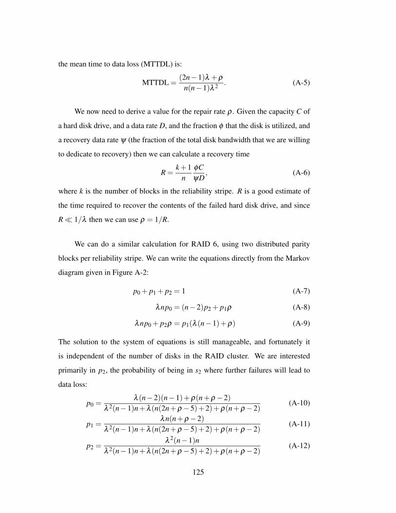
the mean time to data loss (MTTDL) is:

MTTDL =(2n−1)λ +ρ

n(n−1)λ 2 . (A-5)

We now need to derive a value for the repair rate ρ . Given the capacity C of

a hard disk drive, and a data rate D, and the fraction φ that the disk is utilized, and

a recovery data rate ψ (the fraction of the total disk bandwidth that we are willing

to dedicate to recovery) then we can calculate a recovery time

R =k +1

nφCψD

, (A-6)

where k is the number of blocks in the reliability stripe. R is a good estimate of

the time required to recover the contents of the failed hard disk drive, and since

R � 1/λ then we can use ρ = 1/R.

We can do a similar calculation for RAID 6, using two distributed parity

blocks per reliability stripe. We can write the equations directly from the Markov

diagram given in Figure A-2:

p0 + p1 + p2 = 1 (A-7)

λnp0 = (n−2)p2 + p1ρ (A-8)

λnp0 + p2ρ = p1(λ (n−1)+ρ) (A-9)

The solution to the system of equations is still manageable, and fortunately it

is independent of the number of disks in the RAID cluster. We are interested

primarily in p2, the probability of being in s2 where further failures will lead to

data loss:

p0 =λ (n−2)(n−1)+ρ(n+ρ −2)

λ 2(n−1)n+λ (n(2n+ρ −5)+2)+ρ(n+ρ −2)(A-10)

p1 =λn(n+ρ −2)

λ 2(n−1)n+λ (n(2n+ρ −5)+2)+ρ(n+ρ −2)(A-11)

p2 =λ 2(n−1)n

λ 2(n−1)n+λ (n(2n+ρ −5)+2)+ρ(n+ρ −2)(A-12)

125

nλ

ρ

(n - 1)λ (n - 2)λ

ρ

0 1 2 Fail

(a) RAID 6 with failure state

nλ

ρ

(n - 1)λ

ρ

0 1 2

(n - 2)λ

(b) RAID 6 ergodic model

Figure A-2: Markov models for RAID 6 reliability

As with our RAID 5 model, the failure transition for RAID 6 would be taken at

the rate p2(n−2)λ and we can then compute the mean time to data loss:

MTTDL =λ 2(n−1)n+λ (n(2n+ρ −5)+2)+ρ(n+ρ −2)

λ 3(n−2)(n−1)n. (A-13)

If it is decided that RAID 6 with its two distributed parity blocks is insufficient,

then a third parity block could be added. The calculations are similar to those we

have already made.

We can make estimates of the MTTDL, and use that to guide us in the amount

of redundancy required for a given amount of data storage. It seems likely that

there will be several classes of storage. For example, there will be storage to hold

memory images created by checkpoints, and a much larger archive for data that

126

will be kept indefinitely. Studies by Google, and others, have shown that manufac-

turer’s estimates of hard disk drive reliability are overly optimistic [37]. Annual

failure rates (AFR) of from 2% to over 8% were observed, and tended to increase

as the hard disk drives aged. If, for example we pick 6% as an average AFR, then

we can expect a MTTF of 146 000 hours, far short of the 106 hours reported by

many manufacturers. We should also remember that correlated failures are possi-

ble, and so our models based on Markov assumptions are optimistic and provide

only a lower-bound on the amount of redundancy required.

127

B APPENDIX: Uncertainty Quantification for LargeProblems

In this appendix, we discuss some of the computational requirements for uncer-

tainty quantification (UQ). Until now we have been estimating the computing

power to resolve direct simulation of various physical problems. We argue that

equal attention be given to estimating the uncertainty in those solutions from the

combination of model errors and noise in measurements informing the model of

unknown parameter and state values. The goal is the ability of a model, simple or

complex, to utilize experimental information to predict the future development of

the model. We return in a moment to a discussion of the two questions of

1. how many measurements are required for a given model and

2. what are appropriate methods for evaluating the RMS spread in predictions

from a model.

The statistical questions associated with assimilating data to learn uncertain

or unknown fixed parameters and states are compactly addressed by a classical

version of a path integral embodying the flow of the state of the model system

through a period of time in which measurements might be made and through

which the state must be moved forward in time. Using the result of the appli-

cation of Monte Carlo methods to perform this kind of integral for a smaller fluid

dynamics problem, we have a baseline from which to scale the required calcula-

tion to the model sizes discussed just above. Note there are important unresolved

issues in this type of investigation. For example, one does not know ahead of

time if an RMS spread is even a relevant measure of uncertainty if the underlying

distribution has long tails. These types of issues will require further investigation.

129

The model system we consider here is a single layer shallow water equation

on a 100 km by 100 km mid-latitude patch. This kind of fluid dynamics problem

is at the heart of all weather and climate models using for short range or long

term forecasting, and is relevant to problems in the core mission of the DOE. The

model calculation was done on a small, 16 by 16 grid in which the estimated

state and RMS errors for each state were evaluated for three fields: the x and y

horizontal velocity and the height of the fluid. This gives about 1000 dynamical

degrees of freedom (768 to be more precise). Integrating for 4000 time steps

of 36 seconds (0.01 hr) to produce 200,000 Monte Carlo selected paths using

a parallelized Metropolis-Hastings routine on a single NVIDIA GTX 580 GPU

device took 12.3 hours.

Suppose we scale this problem from 103 degrees of freedom to 109 degrees

of freedom, use the same number of accepted paths, time steps, ... and require the

calculation to complete in 10 hours. Then we require 106 GTX 580’s or 5× 108

CUDA cores to accomplish the larger job in the same 10 hours. Realistically,

we also need to scale up the computing requirements for communications among

many GPUs.

One must note that a GTX 580 uses 150 W while performing this compu-

tation, and discounting communications and memory use costs entirely, 150 MW

would be required to use existing GPUs of GTX 580 form factor. That, of course,

is bad news, but in the same ballpark as earlier bad news for the forward com-

puting capability itself, so, in a back of the envelope manner, one might say that

double the compute capability and power consumption estimated for simply scal-

ing up present day computation would be required for exascale computation along

with uncertainty quantification on problems more or less of the size of contempo-

rary numerical weather prediction or climate modeling.

130

There is a thread of estimating uncertainty quantification (UQ) that appears

often in DOE reports and projections going under the name of Wiener-Hermite

expansions [28] or polynomial chaos [56]. The basic idea, due to Weiner in

1938 [52] is this: if we have a field u(x, t) satisfying some partial differential

equation which contains uncertain elements such as transport coefficients or an

uncertain driving force which depends on a fluctuating variable ξ , then we can

expand both the field u(x, t;ξ ) and any parameters as series in orthogonal polyno-

mials φn(ξ )

u(x, t;ξ ) =∞

∑n=0

un(x, t)φn(ξ ) where∫dξ ρ(ξ )φn(ξ )φm(ξ ) = δnm

leading to an infinite number of differential equations among the u j(x, t). Trun-

cating this set yields a reduced set of degrees of freedom to address from which

statistical quantities may be evaluated. The integration measure ρ(ξ ) is selected

to be associated with the specific nature of the noise in the original differential

equations. If that noise is Gaussian then ρ(ξ ) = exp(−ξ 2) and the orthogonal

functions are Hermite polynomials

In papers by Meecham [25], the orthogonality of the polynomials appears

quite attractive as it guarantees that the energy, quadratic in the un(ξ , t) , is a sum

of explicitly positive definite terms

E(k) =k2

(2π)5

∫d3q〈u(k−q, t) ·u(q, t)〉

=(

k2π

)2

|u1(k)|2 +2k2

2π5

∫d3q |u2(k,q− k)|2 + · · ·

and this is a very good attribute.

131

However, truncating the series at a finite order runs afoul of the Marcinkie-

wicz theorem [29] which says that the independent correlations of⟨u(x, t)u(x′, t) . . .u(xn, t(n))

⟩can be truncated at n = 2 when only second order correlations < u(x, t)u(x′, t ′) >

are independent, so the process is Gaussian, or one must keep the full infinite sum

of correlations or the distribution of the dynamical valuables P(u(x, t)) is some-

where negative, contrary to the meaning of a probability distribution. Truncating

the infinite sum in polynomial chaos is a closure approximation which reduces

the infinite number of correlations to a finite number. If that number of indepen-

dent correlations is greater than two, negative probability distributions for the field

u(x, t) will occur. The Hogge and Meecham truncation may well assure the en-

ergy density is positive, but it does not guarantee that the underlying distribution

is everywhere positive, nor can any such finite truncation. The Monte-Carlo eval-

uation of the path integral, which itself is just an integral representation of the full

solution of the original stochastic differential equation never faces this issue as all

moments are present.

Fortunately from a computational perspective, Monte Carlo integration is,

as exemplified by the shallow water equation example, is eminently paralleliz-

able using GPU methods. Once we have a model, we can use it to indicate

how many measurements would be required to estimate any remaining unob-

served state variables and unknown parameters. To accomplish this, we note that

when the data signals yl(t), l = 1,2, . . .L of the corresponding model output sig-

nals xa(t) = 1,2, ...,D (L out of an overall D > L state variables can be compared

to the data) are in synchrony, we may expect that minimizing some distance, say,

Synchronization error =m

∑n=0

L

∑l=1

[yl(tn)− xl(tn)]2

132

will provide the basis for an estimation of any parameters in the problem and the

D-L unobserved state variables. We need all of these parameters and all state

variables at some time to predict beyond that time using our model equations. In

the cases discussed earlier where the flows are chaotic, this is especially important.

What makes it difficult to perform this minimization? When the measured

yl(t) and computed xl(t) are chaotic, the sum is very sensitive to its dependence

on parameters or state variables. The communication of information from the

observations to the model is unstable, and this results in many local minima in the

Synchronization Error sum impeding the ability to search for any minimum.

One can cure this by adding terms k(yl(t)−xl(t)) to the differential equations

for l = 1,2, . . . ,L state variables as one form of communicating information from

measurements to model. As k increases, when L is greater than some critical

value, the instability will be cured and the search surface becomes smooth.

This question can be efficiently explored by generating data from the model

itself, then evaluating the Synchronization Error for new solutions to the model

with different initial conditions and a range of parameters. When L is big enough

and k large enough, synchronization will occur, and the search is made easy.

In the case of the low dimensional shallow water flow discussed above, this

indicates that for a 16× 16 grid, the critical L is about 70% of the number of

degrees of freedom (768 = 2× 16× 16). To determine what this might be for a

model with many, many more degrees of freedom, one would coarse grain the grid

to examine a much smaller number of degrees of freedom, then systematically

refine the grid looking for a trend in L/D where synchronization occurs. For

smaller models this trend sets in quite quickly, and it allows an estimation of the

critical L for large D without actually doing the calculations for large D. It is also

133

true that when the estimations become possible and accurate, the ability to predict

beyond times when observations occur improves dramatically.

134

C APPENDIX: NNSA Application Requirements

In this section we describe application requirements for NNSA stockpile steward-

ship calculations. We also provide an assessment of the possible adverse security

impacts should it prove infeasible to develop an exascale platform by 2020. The

details of this appendix are classified S/RD and so are not distributed with this

unclassified report. The classified appendix is available as a separate document.

135

D APPENDIX: Briefers

Briefer Affiliation Briefing title

Dan Hitchcock, Bob Meisner DOE, NNSA Setting the Stage

Jim Ang SNL Hardware Issues

Rich Murphy SNL Power Issues

Pete Beckman ANL Software Issues

Sriram Swaminarayan LANL RoadRunner Experience

Jim Hack ORNL Getting Ready for Titan

Bert Still LLNL Dawn/Sequoia Experience

Richard Barrett SNL Next-Generation Testbeds

Arun Rodriguez SNL Hardware Simulators

Mike Heroux SNL The Future of MPI

Kathy Yelick LBNL Exascale Programming Challenges

Pat Hanrahan Stanford Domain Specific Languages

Jeff Vetter, Bronis de Supinski ORNL, LLNL Programming Tools

Adolfy Hoisie, Allan Snavely PNNL, LLNL Performance Modeling

Jim Ahrens LANL Data Analytics

John Bell LBNL Combustion

Jim Belak LLNL Materials

Bob Rosner ANL Nuclear Energy

Bruce Goodwin LLNL Overview

Bill Archer LANL LANL Exascale Drivers

Chris Clouse LLNL LLNL NCT Exascale Drivers

Ken Alvin SNL SNL Re-entry Exascale Drivers

David Womble SNL SNL Exascale Applications

Eric Nelson LANL LANL Integrated Design Code

Rob Neeley LLNL LLNL Integrated Design Code

Anne Fitzpatrick DOE/IN HPC Net Assessment

Michael Wehner LBNL The Green Flash Project

137

References

[1] A.M. Aji, J. Dinan, D. Buntinas, P. Balaji, W. Feng, K.R. Bisset, and

R. Thakur. MPI-ACC: An integrated and extensible approach to data move-

ment in accelerator-based systems. In IEEE International Conference on

High Performance Computing and Communications (HPCC), 2012.

[2] Ahmed Amer, JoAnne Holliday, Darrell D. E. Long, Ethan L. Miller, Jehan-

Francois Paris, and Thomas Schwarz. Data management and layout for shin-

gled magnetic recording. IEEE Transactions on Magnetics, 47(10), October

2011.

[3] J. Ang. Hardware issues. Presentation to JASON 2012, June 2012.

[4] K. Asanovic, R. Bodik, B.C. Catanzaro, J.J. Gebis, P. Husbands, K. Keutzer,

D.A. Patterson, W.L. Plishker, J. Shalf, S.W. Williams, et al. The landscape

of parallel computing research: A view from berkeley. Technical report,

UCB/EECS-2006-183, EECS Department, University of California, Berke-

ley, 2006.

[5] J. Bell. Combustion. Presentation to JASON 2012, June 2012.

[6] J. Chan, G. Hendry, A. Biberman, and K. Bergman. Architectural ex-

ploration of chip-scale photonic interconnection network designs using

physical-layer analysis. Journal of Lightwave Technology, 28(9):1305–

1315, 2010.

[7] K.M. Chandy, R. Manohar, B.L. Massingill, and D.I. Meiron. Integrat-

ing task and data parallelism with the collective communication archetype.

Technical report, California Institute of Technology, 1994.

[8] S. H. Charap, P. L. Lu, and Y. He. Thermal stability of recorded information

at high densities. IEEE Transactions on Magnetics, 33(1), January 1997.

139

[9] Jinsuk Chung, Ikhwan Lee, Michael Sullivan, Jee Ho Ryoo, Dong Wan Kim,

Doe Hyun Yoon, Larry Kaplan, and Mattan Erez. Containment Domains: A

Scalable, Efficient, and Flexible Resilience Scheme for Exascale Systems.

In the Proceedings of SC12, November 2012.

[10] Dennis Colarelli and Dirk Grunwald. Massive arrays of idle disks for storage

archives. In Proceedings of the 2002 ACM/IEEE conference on Supercom-

puting, Supercomputing ’02, pages 1–11, Los Alamitos, CA, USA, 2002.

IEEE Computer Society Press.

[11] P. Colella and P.R. Woodward. The piecewise parabolic method (PPM) for

gas-dynamical simulations. Journal of computational physics, 54(1):174–

201, 1984.

[12] C. Constantinescu. Intermittent faults in VLSI circuits. In Proceedings of

the IEEE Workshop on Silicon Errors in Logic-System Effects, 2007.

[13] J.W. Cooley, P.A.W. Lewis, and P.D. Welch. Historical notes on the fast

fourier transform. Proceedings of the IEEE, 55(10):1675–1677, 1967.

[14] I. Corderı and, T. Schwarz, A. Amer, D.D.E. Long, and J-F. Paris. Self-

adjusting two-failure tolerant disk arrays. In Fifth Petascale Data Storage

Workshop (PDSW), pages 1–5, November 2010.

[15] P.W. Coteus, J.U. Knickerbocker, C.H. Lam, and Y.A. Vlasov. Technologies

for exascale systems. IBM Journal of Research and Development, 55(5):14–

1, 2011.

[16] Tom Coughlin and Ed Grochowski. 2012–2016 capital equipment and tech-

nology report for the hard disk drive industry. Technical report, Coughlin

Associates, February 2012.

[17] J.E. Cunningham, I. Shubin, X. Zheng, T. Pinguet, A. Mekis, Y. Luo,

H. Thacker, G. Li, J. Yao, K. Raj, et al. Highly-efficient thermally-tuned

resonant optical filters. Opt. Express, 18(18):19055–19063, 2010.

140

[18] R. et al Dennard. Design of ion-implanted MOSFET’s with very small phys-

ical dimensions. IEEE J. Solid State Circuits, 1974.

[19] Z. DeVito, N. Joubert, F. Palacios, S. Oakley, M. Medina, M. Barrientos,

E. Elsen, F. Ham, A. Aiken, K. Duraisamy, et al. Liszt: a domain specific

language for building portable mesh-based PDE solvers. In Proceedings of

2011 International Conference for High Performance Computing, Network-

ing, Storage and Analysis, page 9, 2011.

[20] M. Frigo and S.G. Johnson. The design and implementation of FFTW3.

Proceedings of the IEEE, 93(2):216–231, February 2005.

[21] Samuel H. Fuller and Editors; Committee on Sustaining Growth in Com-

puting Performance; National Research Council Lynette I. Millett. The Fu-

ture of Computing Performance: Game Over or Next Level? The National

Academies Press, 2011.

[22] Laura M. Grupp, John D. Davis, and Steven Swanson. The bleak future of

NAND flash memory. In Proceedings of the 10th USENIX Conference on

File and Storage Technologies (FAST), February 2012.

[23] P. Hazucha, T. Karnik, J. Maiz, S. Walstra, B. Bloechel, J. Tschanz, G. Der-

mer, S. Hareland, P. Armstrong, and S. Borkar. Neutron soft error rate mea-

surements in a 90-nm CMOS process and scaling trends in SRAM from

0.25 µm to 90 nm generation. In Electron Devices Meeting, 2003. IEDM’03

Technical Digest. IEEE International, page 215, 2003.

[24] M. Heroux. The future of MPI. Presentation to JASON 2012, June 2012.

[25] HD Hogge and WC Meecham. The wiener-hermite expansion applied to de-

caying isotropic turbulence using a renormalized time-dependent base. Jour-

nal of Fluid Mechanics, 85:325–347, 1978.

[26] S.W. Keckler, W.J. Dally, B. Khailany, M. Garland, and D. Glasco. Gpus

and the future of parallel computing. Micro, IEEE, 31(5):7–17, 2011.

141

[27] Peter Kogge, Keren Bergman, Shekhar Borkar, Dan Campbell, William

Carlson, William Dally, Monty Denneau, Paul Franzon, William Harrod,

Kerry Hill, Jon Hiller, Sherman Karp, Stephen Keckler, Dean Klein, Robert

Lucas, Mark Richards, Al Scarpelli, Steven Scott, Allan Snavely, Thomas

Sterling, R. Stanley Williams, and Katherine Yelick. ExaScale computing

study: Technology challenges in achieving exascale systems. Technical re-

port, DARPA, 2008.

[28] C.P. Lee, W.C. Meecham, and HD Hogge. Application of the wiener–

hermite expansion to turbulence of moderate reynolds number. Physics of

Fluids, 25:1322, 1982.

[29] J. Marcinkiewicz. Sur une propriete de la loi de gauss. Mathematische

Zeitschrift, 44(1):612–618, 1939.

[30] S.E. Michalak, K.W. Harris, N.W. Hengartner, B.E. Takala, and S.A. Wen-

der. Predicting the number of fatal soft errors in los alamos national labora-

tory’s ASC q supercomputer. IEEE Transactions on Device and Materials

Reliability, 5(3):329–335, September 2005.

[31] Gordon E. Moore. Cramming more components onto integrated circuits.

Electronics Magazine, 1965.

[32] R. Murphy. Power issues. Presentation to JASON 2012, June 2012.

[33] Richard Murphy, Arun Rodrigues, Peter Kogge, and Keith Underwood. The

implications of working set analysis on supercomputing memory hierarchy

design. In Proceedings of the 19th ACM International Conference on Super-

computing, Cambridge, MA, 2005. ACM.

[34] K. Olukotun and L. Hammond. The future of microprocessors. Queue,

3(7):26–29, 2005.

[35] Ophir, Bergman, and Mines. A silicon photonic microring link case study

for high-bandwidth density low-power chip I/O. draft in preparation, 2008.

142

[36] A. Petitet, R.C. Whaley, J. Dongarra, and A. Cleary. HPL-a portable im-

plementation of the high-performance linpack benchmark for distributed-

memory computers. Version 1.0 a, 2004.

[37] Eduardo Pinheiro, Wolf-Dietrich Weber, and Luiz Andre Barroso. Failure

trends in a large disk drive population. In Proceedings of the 5th USENIX

conference on File and Storage Technologies, FAST ’07, pages 2–2, Berke-

ley, CA, USA, 2007. USENIX Association.

[38] Rambus. Challenges and solutions for future main memory, 2009.

[39] C. Rowen. www.tensilica.com.

[40] C.L. Schow, A.V. Rylyakov, C. Baks, F.E. Doany, and J.A. Kash. 25-gb/s

6.5-pJ/bit 90-nm cmos-driven multimode optical link. Photonics Technology

Letters, IEEE, 24(10):824–826, 2012.

[41] B. Schroeder, E. Pinheiro, and W. D. Weber. DRAM errors in the wild: a

large-scale field study. In Proceedings of the eleventh international joint con-

ference on Measurement and modeling of computer systems, page 193204,

2009.

[42] Bianca Schroeder and Garth A Gibson. A large-scale study of failures in

high-performance computing systems. IEEE Transactions on Dependable

and Secure Computing, 7(4):337–350, October 2010.

[43] Sandeep Shah and Jon G. Elerath. Disk drive vintage and its effect on relia-

bility. In Proceedings of 2004 Annual Reliability and Maintainability Sym-

posium, pages 163–165. IEEE, 2004.

[44] D.E. Shaw, M.M. Deneroff, R.O. Dror, J.S. Kuskin, R.H. Larson, J.K.

Salmon, C. Young, B. Batson, K.J. Bowers, J.C. Chao, et al. Anton,

a special-purpose machine for molecular dynamics simulation. In ACM

SIGARCH Computer Architecture News, volume 35, pages 1–12. ACM,

2007.

143

[45] G. R. Srinivasan. Modeling the cosmic-ray-induced soft-error rate in inte-

grated circuits: an overview. IBM Journal of Research and Development,

40(1):7789, 1996.

[46] B. Still. Dawn/sequoia experience. Presentation to JASON 2012, June 2012.

[47] H. H. K. Tang. Nuclear physics of cosmic ray interaction with semiconductor

materials: particle-induced soft errors from a physicist’s perspective. IBM

journal of research and development, 40(1):91108, 1996.

[48] D. Turek. High performance computing and the implications of multi-core

architectures. CTWatch Quarterly, 3(1):31–33, 2007.

[49] J. Vetter. Programming tools. Presentation to JASON 2012, June 2012.

[50] M. Wehner. The Green Flash project. Presentation to JASON 2012, July

2012.

[51] Michael Wehner, Leonid Oliker, and John Shalf. Towards ultra-high resolu-

tion models of climate and weather. International Journal of High Perfor-

mance Computing Applications, 2008.

[52] N. Wiener. The homogeneous chaos. American Journal of Mathematics,

60(4):897–936, 1938.

[53] Rick Dee et al Williams. JEDEC server memory roadmap. Technical report,

JEDEC, 2011.

[54] Samuel Williams, Andrew Waterman, and David Patterson. Roofline: An in-

sightful visual performance model for floating-point programs and multicore

architectures. submitted to Communications of the ACM, 2008.

[55] Qin Xin, Ethan L. Miller, Thomas Schwarz, Darrell D. E. Long, Scott A.

Brandt, and Witold Litwin. Reliability mechanisms for very large storage

systems. In Proceedings of the 20th IEEE / 11th NASA Goddard Conference

on Mass Storage Systems and Technologies, pages 146–156, April 2003.

144

[56] D. Xiu and G. Em Karniadakis. Modeling uncertainty in steady state dif-

fusion problems via generalized polynomial chaos. Computer Methods in

Applied Mechanics and Engineering, 191(43):4927–4948, 2002.

[57] K. Yelick. Exascale programming model challenges. Presentation to JASON

2012, June 2012.

[58] J. F. Ziegler. Terrestrial cosmic rays. IBM Journal of Research and Devel-

opment, 40(1):1939, 1996.

145