Tdyn Tutorials - Compass · PDF fileTdyn Tutorials Compass Ingeniería ... Taylor-Couette flow 168 Introduction 168 ... The actual value of the Reynolds number is taken to be Re =

Environment for multi-physics simulation, including fluid dynamics, turbulence, advection of species, structural mechanics, free surface and user defined PDE solvers.

Tdyn Tutorials

Compass Ingeniería y Sistemas http://www.compassis.comTel.: +34 932 181 989 - Fax.: +34 933 969 746 - E: [email protected] - C/ Tuset 8, 7o 2a, Barcelona 08006 (Spain)

Table of Contents

Tdyn Tutorials

iiCompass Ingeniería y Sistemas - http://www.compassis.com

Chapters Pag.

Tutorials list 1

Cavity flow 13

Introduction 13

Start data 14

Pre-processing 14

Boundary conditions 15

Materials 16

Boundaries 17

Problem data 18

Mesh generation 20

Calculate 21

Post-processing 21

Graphs 23

Cavity flow, heat transfer 25

Introduction 25

Start data 25

Pre-processing 26


Materials 26

Boundaries 27

Problem data 28

Mesh generation 29

Calculate 29

Post-processing 29

Three-dimensional flow passing a cylinder 32

Introduction 32

Start data 33

Pre-processing 33

Initial data 35


Tdyn Tutorials

iiiCompass Ingeniería y Sistemas - http://www.compassis.com

Materials 37

Boundaries 38

Problem data 39

Mesh generation 40

Calculate 40

Post-processing 40

Advanced tutorials 44

Two-dimensional flow passing a cylinder 44

Introduction 44

Start data 45

Pre-processing 45

Initial data 47


Materials 48

Boundaries 49

Problem data 49

Mesh generation 50

Calculate 50

Post-processing 51

Backward facing step 57

Introduction 57

Start data 57

Pre-processing 58

Initial data 58


Materials 61

Boundaries 62

Problem data 62

Mesh generation 63

Calculate 64

Post-processing 64

Heat transfer analysis of a solid 66

Tdyn Tutorials

ivCompass Ingeniería y Sistemas - http://www.compassis.com

Introduction 66

Start data 67

Pre-processing 67


Materials 68

Problem data 68

Mesh generation 68

Calculate 69

Post-processing 69

Species advection 70

Introduction 70

Start data 70

Pre-processing 71

Initial data 71

Materials 72


Problem data 75

Mesh generation 76

Calculate 76

Post-processing 76

ALE Cylinder 79

Introduction 79

Start data 79

Pre-processing 79

Initial data 79


Boundaries 80

Modules data 81

Problem data 81

Calculate 82

Post-processing 82

Fluid-Solid thermal contact 84

Tdyn Tutorials

vCompass Ingeniería y Sistemas - http://www.compassis.com

Introduction 84

Start data 84

Pre-processing 84


Materials 86

Boundaries 87

Contacts 87

Problem data 90

Mesh generation 90

Calculate 90

Post-processing 90

Analysis of an electric motor 92

Introduction 92

Start data 93

Pre-processing 93


Materials 94

Problem data 97

Mesh generation 98

Calculate 98

Post-processing 98

Analysis of a dam break (ODD level set) 100

Introduction 100

Start data 101

Pre-processing 101

Initial data 101

Materials 103

Boundaries 103

Problem data 104

Modules data 104

Mesh generation 105

Calculate 105

Tdyn Tutorials

viCompass Ingeniería y Sistemas - http://www.compassis.com

Post-processing 106

Compressible flow around NACA airfoil 107

Introduction 107

Start data 107

Pre-processing 107

Initial data 108


Materials 109

Boundaries 111

Problem data 111

Modules data 112

Mesh generation 112

Calculate 112

Post-processing 113

3D Cavity flow 115

Introduction 115

Start data 116

Pre-processing 116


Materials 118

Boundaries 119

Problem data 120

Mesh generation 121

Calculate 122

Post-processing 122

Laminar flow in pipe 125

Introduction 125

Start data 125

Pre-processing 126


Materials 127

Boundaries 127

Tdyn Tutorials

viiCompass Ingeniería y Sistemas - http://www.compassis.com

Problem data 127

Mesh generation 128

Calculate 129

Post-processing 129

Turbulent flow in pipe 131

Introduction 131

Start data 131

Pre-processing 132


Materials 132

Boundaries 132

Problem data 133

Modules data 133

Mesh generation 133

Initial data 135

Calculate 135

Post-processing 135

Appendix 138

Laminar and turbulent flows in a 3D pipe 139

Introduction 139

Start data 139

Pre-processing 139


Materials 141

Boundaries 141

Problem data 142

Modules data 142

Mesh generation 143

Initial data 147

Calculate 147

Post-processing 148

Ekman's Spiral 151

Tdyn Tutorials

viiiCompass Ingeniería y Sistemas - http://www.compassis.com

Introduction 151

Start data 153

Pre-processing 154


Materials 157

Problem data 158

Modules data 159

Mesh generation 159

Calculate 160

Post-processing 160

Appendix (TCL script) 163

Taylor-Couette flow 168

Introduction 168

Start data 170

Pre-processing 170


Materials 173

Problem data 174

TCL extension 175

Mesh generation 176

Calculate 177

Post-processing 178

Appendix 1 181

Appendix 2 182

Heat transfer analysis of a 3D solid 184

Introduction 184

Start data 184

Pre-processing 185

Initial data 185

Materials 185

Boundaries 186

Problem data 187

Tdyn Tutorials

ixCompass Ingeniería y Sistemas - http://www.compassis.com

Mesh generation 187

Calculate 188

Post-processing 188

Towing analysis of a wigley hull 190

Introduction 190

Start data 191

Pre-processing 191

Initial data 195


Materials 197

Boundaries 198

Problem data 200

Modules data 201

Mesh generation 201

Calculate 201

Post-processing 203

Appendix 209

Wigley hull in head waves 215

Introduction 215

Start data 215

Pre-processing 215

Problem data 217

Modules data 218

Initial data 219

Boundaries 220

Materials 222

Mesh generation 223

Calculate 223

Post-processing 223

Appendix 224

Thermal contact between two solids 225

Introduction 225

Tdyn Tutorials

xCompass Ingeniería y Sistemas - http://www.compassis.com

Start data 225

Pre-processing 225


Materials 226

Contacts 227

Problem data 229

Mesh generation 230

Calculate 230

Post-processing 230

Fluid-Structure interaction 232

Introduction 232

Start data 232

Pre-processing 232

General data 236

Coupling data 237


Materials 239

Structural loads 241

Problem data 243

Mesh generation 244

Calculate 247

Post-processing 247

Potential flow with free surface 249

Introduction 249

Problem formulation 249

Start data 251

Pre-processing 251

Problem data 251

Materials 252


Mesh generation 261

Calculate 261

Tdyn Tutorials

xiCompass Ingeniería y Sistemas - http://www.compassis.com

Post-processing 261

2D Sloshing Test 263

Introduction 263

Start Data 263

Pre-processing 263

Problem data 264

Modules data 265

Initial data 266

Materials 267

Boundaries 268

Mesh generation 270

Post-processing 272

2D air quality modeling 276

Introduction 276

Start Data 276

Pre-processing 276

Initial Data 277


Materials 280

Problem data 282

Mesh generation 283

Calculate 283

Post-processing 284

References 287

1 Tutorials list

Tdyn Tutorials

1Compass Ingeniería y Sistemas - http://www.compassis.com

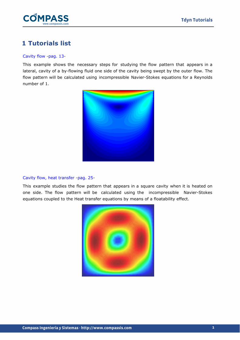
Cavity flow -pag. 13-

This example shows the necessary steps for studying the flow pattern that appears in a lateral, cavity of a by-flowing fluid one side of the cavity being swept by the outer flow. The flow pattern will be calculated using incompressible Navier-Stokes equations for a Reynolds number of 1.

Cavity flow, heat transfer -pag. 25-

This example studies the flow pattern that appears in a square cavity when it is heated on one side. The flow pattern will be calculated using the incompressible Navier-Stokes equations coupled to the Heat transfer equations by means of a floatability effect.

Tdyn Tutorials


Backward facing step -pag. 57-

This example is a two-dimensional study of a fluid flow within a channel with a backward-facing step. The flow pattern will be calculated using the incompressible Navier-Stokes equations for a Reynolds number in the laminar range.

Two-dimensional flow passing a cylinder -pag. 44-

This tutorial concerns the two-dimensional flow passing a cylinder in the low Reynolds number range. The actual value of the Reynolds number is taken to be Re = 100, for which a vortex street in the wake of the cylinder is expected.

Heat transfer analysis of a solid -pag. 66-

This example illustrates the heat transfer problem in a solid that is heated on one side while it is being cooled on the other.

Tdyn Tutorials


Species advection -pag. 70-

This tutorial concerns the transport problem of two species in a squared domain. Such a species transport is produced by the advection in a fluid that is moving with a constant velocity given by the vector (1.0,1.0,0.0) m/s.

ALE Cylinder -pag. 79-

This tutorial simulates a cylinder moving with uniform velocity through a fluid at rest. The resulting global Reynolds number is Re=100. This kind of analysis requires the mesh to be updated every time step. In order to solve this problem we will use the capabilities of the ALEMESH module.

Tdyn Tutorials


Fluid-Solid thermal contact -pag. 84-

This example studies the flow pattern that appears in a square cavity when it is heated on one side, in contact with a hot solid.

Analysis of an electric motor -pag. 92-

This example studies the 2D static magnetic field due to the stator winding in a two-pole electric motor.

Tdyn Tutorials


Analysis of a dam break (ODD level set) -pag. 100-

This example studies the 2D water evolution in a dam break process, and the encounter of the fluid with two obstacles.

Compressible flow around NACA airfoil -pag. 107-

This example shows the necessary steps for studying the flow pattern about a NACA profile. The flow pattern will be calculated using the compressible Navier-Stokes equations for a Mach number of 0.5.

Tdyn Tutorials


3D Cavity flow -pag. 115-

This example shows the necessary steps for studying the flow pattern that appears in a "lateral", cavity of a by-flowing fluid, one side of the cavity being swept by the outer flow. The flow pattern will be calculated using the incompressible Navier-Stokes equations for a Reynolds number of 1.

Laminar flow in pipe -pag. 125-

This example shows the analysis of a fluid flowing through a circular pipe of constant cross-section. The Reynolds number is Re=100.

Tdyn Tutorials


Turbulent flow in pipe -pag. 131-

This example shows the analysis of a fluid flowing through a circular pipe of constant cross-section. The Reynolds number is Re=20000.

Laminar and turbulent flows in a 3D pipe -pag. 139-

This tutorial is a 3D extension of the previous 2D examples which concerned the analysis of laminar and turbulent flows in a pipe.

Tdyn Tutorials


Example 16 - Ekman's Spiral

The application of TCL script programming in CompassFEM_FD&M is discussed in this tutorial. The case study chosen for the sake of illustration is the solution of the Ekman's spiral.

Taylor-Couette flow -pag. 168-

The Taylor-Couette experiment consists on a fluid filling the gap between two concentric cylinders, one of them rotating around their common axis.

Tdyn Tutorials


Three-dimensional flow passing a cylinder -pag. 32-

This tutorial analyses the case of a three-dimensional flow passing a cylinder in the low Reynolds number range (Re = 100), for which we expect a vortex street in the wake of the cylinder (the well known von Kármán vortex street).

Heat transfer analysis of a 3D solid -pag. 184-

This tutorial concerns the analysis of a solid that is cooling down from its bulk temperature to the temperature of the surrounding media.

Tdyn Tutorials


Towing analysis of a wigley hull -pag. 190-

This example shows the necessary steps for the hydrodynamic calculation of the so-called Wigley hull, with a Froude number Fr=0.316 using the NAVAL capabilities of the CompassFEM suite.

Wigley hull in head waves -pag. 215-

This example illustrates the analysis of a Wigley hull in head waves using ODDLS module. The analysis will be carried out with the ship moving forward with a Froude number Fr = 0.316.

Tdyn Tutorials


Thermal contact between two solids -pag. 225-

This tutorial concerns the heat transfer problem between two solid boxes in contact.

Fluid-Structure interaction -pag. 232-

This tutorial illustrates the fluid-structure interaction capabilities of Tdyn for the particular case of a 3D flexible solid structure in a channel with a gradual contraction.

Potential flow with free surface -pag. 249-

This example shows the necessary steps to analyse the potential flow about a cylinder with linear free surface condition. The formulation of the free surface condition will be done using TdynTcl extension available in URSOLVER module.

Tdyn Tutorials


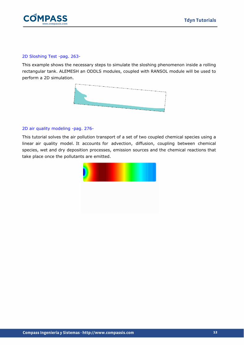
2D Sloshing Test -pag. 263-

This example shows the necessary steps to simulate the sloshing phenomenon inside a rolling rectangular tank. ALEMESH an ODDLS modules, coupled with RANSOL module will be used to perform a 2D simulation.

2D air quality modeling -pag. 276-

This tutorial solves the air pollution transport of a set of two coupled chemical species using a linear air quality model. It accounts for advection, diffusion, coupling between chemical species, wet and dry deposition processes, emission sources and the chemical reactions that take place once the pollutants are emitted.

2 Cavity flow

Tdyn Tutorials


Introduction

This example shows the necessary steps for studying the flow pattern that appears in a lateral, cavity of a by-flowing fluid one side of the cavity being swept by the outer flow. The flow pattern will be calculated using incompressible Navier-Stokes equations for a Reynolds number of 1 (in order to capture turbulence effects that appear at higher Reynolds numbers, a finner mesh would be necessary).

The geometry simply consists of a square, representing a cavity, its top face being swept by the passing fluid. This problem is a two-dimensional case solved to illustrate the basic capabilities of Tdyn.

Schema of the 2D cavity flow problem.

The Reynolds number is defined as Re = ρvL/μ.In this equation, L represents the characteristic length of the problem, which in this case is the edge length of the cavity, ρ and μ are the density and the viscosity of the fluid respectively, and v is the velocity of the flow on the swept line. For the example to be solved here, we can choose arbitrarily:

L = 1.0 m

v = 1.0 m/s

ρ = 1.0 kg/m3

μ = 1.0 kg/ms

By substituting the variables for their value in the equation above we obtain the Reynolds number Re = 1.

Tdyn Tutorials


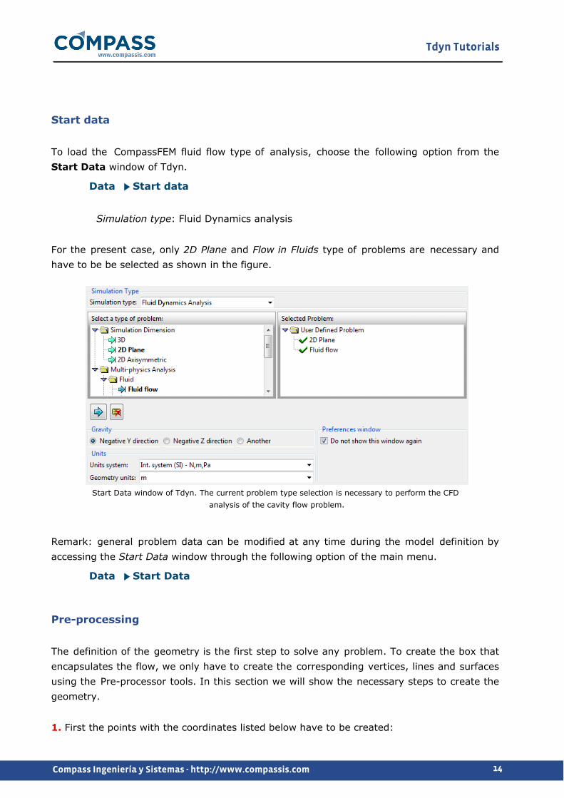
Start data

To load the CompassFEM fluid flow type of analysis, choose the following option from the Start Data window of Tdyn.

Data Start data

Simulation type: Fluid Dynamics analysis

For the present case, only 2D Plane and Flow in Fluids type of problems are necessary and have to be be selected as shown in the figure.

Start Data window of Tdyn. The current problem type selection is necessary to perform the CFD analysis of the cavity flow problem.

Remark: general problem data can be modified at any time during the model definition by accessing the Start Data window through the following option of the main menu.

Data Start Data

Pre-processing

The definition of the geometry is the first step to solve any problem. To create the box that encapsulates the flow, we only have to create the corresponding vertices, lines and surfaces using the Pre-processor tools. In this section we will show the necessary steps to create the geometry.

1. First the points with the coordinates listed below have to be created:

Tdyn Tutorials


Point number X Coordinate Y Coordinate

1 0.000000 0.000000

2 1.000000 0.000000

3 1.000000 1.000000

4 0.000000 1.000000

Geometry Create Point

- Enter point coordinates in the command line.

2. Then the lines have to be created joining the corresponding points. Use the following option (use Join or Ctrl+A to catch already existing points with the mouse button).

Geometry Create Straight line

- Select the two points defining each line

3. Once all the lines have been created, the surface that must represent the cavity (i.e. the control domain) has to be created.

Geometry Create NURBS surface By contour

- Select the four lines that define the contour of the square domain.

4. It is important to note here that the surface normals must be oriented in the OZ positive sense. This may be checked using the following option from the main menu.

View Normals Surfaces

- Select the surface or surfaces whose normals must be checked.

5. If you need to change the orientation of a normal, use the following menu sequence,

Utilities Swap Normals Surfaces

- Select the surface or surfaces whose normals are going to be swapped.

Boundary conditions

Once we have defined the geometry, it is necessary to set the boundary conditions of the problem. This process is carried out through the Conditions & Initial Data section of the CompassFEM Data tree. The only conditions to specify here are:

Tdyn Tutorials


Conditions & Initial Data Fluid Flow Fix Velocity

Conditions and Initial Data Fluid Flow Fix Pressure

a) Fix velocity [line]

This condition is used to impose the velocity on a line. The fields in the values tab of the Fix Velocity condition window store the velocity components (X and Y) given in global axes. The flags Fix X Velocity and Fix Y Velocity in the activation tab of the window allow to indicate if the corresponding components have to be fixed or not. If the corresponding Fix flag is not selected, the corresponding values field will be disabled. In the present example this condition is going to be assigned to the line swept by the flow. In our case, the X-component of the velocity vector will be set to 1.0 m/s, and the Y-component to zero. Then, all the velocity components have to be fixed to the specified value (i.e. mark Fix X Velocity and Fix Y Velocity) as shown in the figure below.

b) Fix Pressure [Point]

In most cases, it is recommended to fix the pressure at least in one point of the control domain (taken as reference). If this condition is not applied, Tdyn makes some corrections and the solution of the problem is equally achieved most of the times. In this case, the Fix Pressure condition will be applied to the bottom left corner.

Materials

Physical properties of the materials used in the problem are defined through the following

Tdyn Tutorials


section of the CompassFEM Data tree.

Materials Physical Properties

If necessary, new materials can be created. In the Fluid Flow list of properties, density and viscosity of the fluid are fixed to 1 Kg/m3and 1 Kg/m·s respectively. For every parameter, the corresponding units have to be verified, and changed if necessary (in our example, all the values are given in default units).

Note that many of the options have specific on-line help that can be accessed by clicking on them with the right button of the mouse.

Materials are finally assigned through the

Materials Fluid

section of the data tree. In this example the material has to be assigned to the created surface that defines the cavity.

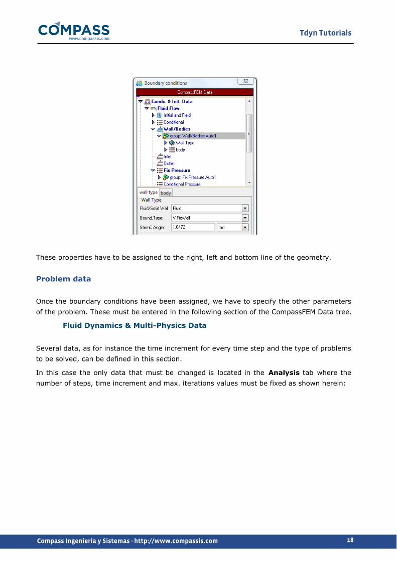
Boundaries

Fluid Wall/Bodies

Fluid wall and bodies are used to define fluid boundary properties in an automatic way. In the Post-processing part, forces on Fluid Body can be drawn. If necessary, new fluid boundaries can be created, based on the existing ones.

In the present case, the values have to be fixed as shown in the figure.

Tdyn Tutorials


These properties have to be assigned to the right, left and bottom line of the geometry.

Problem data

Once the boundary conditions have been assigned, we have to specify the other parameters of the problem. These must be entered in the following section of the CompassFEM Data tree.

Fluid Dynamics & Multi-Physics Data

Several data, as for instance the time increment for every time step and the type of problems to be solved, can be defined in this section.

In this case the only data that must be changed is located in the Analysis tab where the number of steps, time increment and max. iterations values must be fixed as shown herein:

Tdyn Tutorials


Within this section, it is also possible to define solver properties (see FLUID SOLVER and SOLID SOLVER tags) and symmetry planes (see OTHER tag) for example. These options will not be changed in this example.

Following are explanations of the most useful options:

Option Meaning

Number of steps Number of steps of the simulation. Total time of the simulation will be (Number_of_Steps X Time_increment).

Max Iterations Maximum number of iterations of the non-linear fluid scheme (recommended values 1-3).

Time increment Time increment for each time step (recommended values < 0.1 * Length / Velocity).

Output Step Each Output_Step time steps the results will be written.

Output Start Results will be written after Output_Start time steps.

A brief summary of the boundary conditions, boundary definitions and material properties that have been applied to the control domain are given in what follows:

Tdyn Tutorials


Condition Entity

Fix Velocity Line 3

Fluid Wall Line 1, 2, 4

Fluid Surface 1

Fix Pressure Point 1

Mesh generation

Size Assignment

The size of the elements generated is of critical importance. Too big elements can lead to bad quality results, whereas too small elements can dramatically increase the computational time without significant improvement of the quality of the results.

In order to generate the mesh select the following option in the main menu. It can also be accessed through the (Ctrl+g) shortcut.

Mesh Generate mesh

You will then be asked for the global element size. In this case, a global element size about 0.0185 was used so that the final mesh contains about the maximum number of nodes allowed by the limited version of Tdyn.

The outcome is the unstructured mesh shown in the Figure below, consisting of 3418 nodes and 6834 triangular elements.

Tdyn Tutorials


Calculate

Calculate

Once the geometry is created, the boundary conditions are applied and the mesh has been generated, we can proceed to solve the problem. Through the Calculate menu, we can start the solution process from within GiD. When pressing the Start button in the Calculate window, GiD will first write the calculation file called ProblemName.flavia (ProblemName being the name under which the problem has been saved in GiD), and then the process will start. This can be done automatically by using the corresponding icon.

Once the solution process is completed, we can visualise the results using Post-processor module. The results file ProblemName.flavia.res will be loaded when selecting the Post-process option.

Post-processing

Once the message Process '...' started on ... has finished is displayed, we can visualise the final results by pressing Post-process (note that the problem must still be loaded; should this not be the case we first have to open the problem files again). Note that the intermediate results can be shown in any moment of the process, even if the calculations are not finished.

The main post process window couples various sets of options, such as animations control, meshes, results or preferences selectors. In this way, each set of these options can be

Tdyn Tutorials


opened or minimized by pressing on its own grey rectangular button, which is located vertically at the left side of the post process window. For further details on postprocessing options see the Postprocess reference manual

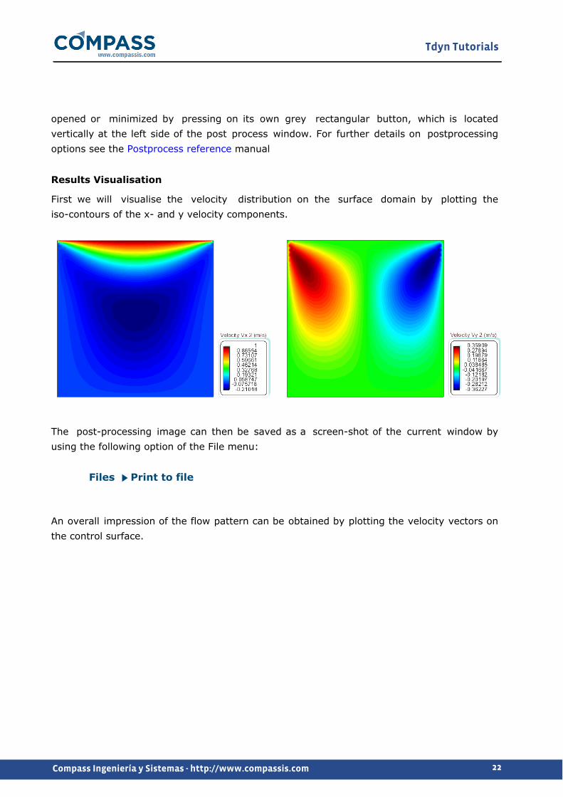
Results Visualisation

First we will visualise the velocity distribution on the surface domain by plotting the iso-contours of the x- and y velocity components.

The post-processing image can then be saved as a screen-shot of the current window by using the following option of the File menu:

Files Print to file

An overall impression of the flow pattern can be obtained by plotting the velocity vectors on the control surface.

Tdyn Tutorials


Finally, we can also plot the pressure distribution over the cut plane.

Graphs

As the graphs will be visualised over a cross section only, we have to proceed by cutting the mesh at the desired position. To do the cut, the following menu option must be applied

Postprocess Create cut plane

Tdyn Tutorials


The cut plane will be perpendicular to the view drawn on the screen. In order to select the nodes of the mesh you can introduce points, either with the mouse or by introducing their co-ordinates manually in the Create cut plane/line window. In this example we will select a cut plane parallel to the original orientation of the control volume (XY-plane). In our case we used the points (0.0, 0.5) and (1.0, 0.5).

By leaving only the cuts on we can plot and visualise the results over the cross section. Graphs can be easily drawn using the Line graph option of the contextual menu that can be accessed by right-clicking on the screen over the line cut. The currently selected result is plotted in the new graph. The resultant plot is shown in the following figure.

For more details on the post-processing steps, please refer to the Pre/Post-processor user manual, or to the online help from the Help menu.

3 Cavity flow, heat transfer

Tdyn Tutorials


Introduction

Introduction

This example studies the flow pattern that appears in a square cavity when it is heated on one side.

This case study is based on the previous example, and the same geometry will be used.

The flow pattern will be calculated using the incompressible Navier-Stokes equations coupled to the heat transfer equations by means of a floatability effect. Such an effect is controlled by the volume expansion coefficient property of the fluid so that the floatability is taken to be proportional to the temperature (in the present case floatability = 0.1·T). The fluid properties controlling the flow behavior are as follows:

Density : ρ = 1.0 kg/m3

Viscosity : μ = 1.0 kg/m·s

Specific heat : c = 10.0 J/Kg·Cº

Thermal conductivity : k = 1.0 W/m·Cº

Start data

In this case, it is necessary to load the following types of problem in the Start Data window of the CompassFEM suite.

Tdyn Tutorials


2D Plane Flow in fluids Heat transfer in fluids

See the Start Data section of the Cavity flow problem (tutorial 1) for details.

Pre-processing

The geometry simply consists of a square, representing a cavity. This problem is a two-dimensional case solved to illustrate the basic capabilities of the Fluid Dynamics and Multiphysics module of the CompassFEM suite.

The best way to proceed from example 1 is to save this file with a different name. Then select again the CompassFEM problemtype and update the model when asked.

Data Problem Type CompassFEM

This will preserve the geometry while deleting all the conditions of the problem.

Boundary conditions

Once we have defined the geometry of the control volume, it is necessary to set the corresponding boundary conditions. The only condition to specify here is a Fix Temerature condition along a line.

Conditions & Initial Data Heat Transfer Fix Temperature

a) Fix Temperature [line]

The Fix Temperature [line] condition is used to fix the temperature on a line. In this example this condition will be assigned to the left line of the geometry with the value 100 ºC and to the right line with the value 0ºC.

Materials

Materials (Fluid)

In this example, fluid properties have to be fixed as follows:

Materials Physical Properties Generic Fluid Generic Fluid 1

Tdyn Tutorials


Fluid flow properties

Thermal properties

Note that the Floatability field defines the coupling effect between fluid and thermal flow.

Materials are finally assigned to the only existing surface of the domain.

Materials Fluid Assign Fluid GenericFluid_1

Boundaries

Fluid Wall/Bodies

Tdyn Tutorials


In this case a V FixWall boundary condition must be selected for the Fluid Wall definition (see figure below).

This property has to be assigned to all the contour lines of the geometry.

Problem data

Once the boundary conditions have been assigned, we have to specify the other parameters of the problem. These must be entered in the following section of the CompassFEM Data tree. In the present case the analysis data should be fixed as follows:

Fluid Dynamics & Multi-Physics Data Analysis

Number of steps 100

Time increment 0.1 s

Max. iterations 3

Initial steps 0

Steady State solver Off

A brief summary of the boundary conditions, boundary definitions and material properties that have been applied to the control domain is given in what follows:

Condition Value Entity

Tdyn Tutorials


Fix Temperature Line 0 Line 2

Fix Temperature Line 100 Line 4

Fluid Body - Line 1, 2, 3, 4

Fluid - Surface 1

Mesh generation

The mesh to be used in this example will be identical to that generated in example 1 (global element size 0.1).

Calculate

The calculation process will be started from within GiD through the Calculate menu, exactly as described in the previous example.

Post-processing

When the calculations are finished, a message Process'...' started on ... has finished is displayed. Then we can proceed to visualising the results by pressing Postprocess (therefore the problem must still be loaded; should this not be the case we first have to open the problem files again).

As the post-processing options to be used are the same as in the previous example, they will not be described in detail here again. For further information please refer to the

Tdyn Tutorials


Postprocessing chapter of previous example and to the Pre/Postprocessor user manual or online help. The results given below correspond to the last time step of t = 10s.

Thermal distribution

Pressure distribution

Tdyn Tutorials


Velocity distribution

Velocity vector field distribution

4 Three-dimensional flow passing a cylinder

Tdyn Tutorials


Introduction

The next example of this tutorial analyses another case in the low Reynolds number range. The problem at hand is a three-dimensional extension of the model presented in a former chapter of this tutorial (see Two-dimensional flow passing a cylinder -pag. 44-). As in the 2D case, we have choosen a Reynolds number Re = 100, for which we expect a vortex street in the wake of the cylinder (the well known von Kármán vortex street).

As usual, the model consists of a control volume, which contains the body under analysis that in this case is a circular cylinder. The geometry of the model is sketched in the following figure.

In order to run the problem within the low Reynolds number range, the following parameters were choosen to set up the model:

D = 1 m

v = 1 m/s

ρ = 1 kg/m3

μ = 1·10-2 kg/m·s

Therefore the Reynolds number becomes Re = 100.

Tdyn Tutorials


Under this conditions the characteristics of the flow are:

- Flow passing a cylinder

- Viscous, non-turbulent flow

- Reynolds number of 100

Start data

For this case, the following type of problems must be loaded in the Start Data window of the CompassFEM suite.

3D Plane Flow in fluids


Pre-processing

Again the geometry for this example is created using the Pre-processor. First we have to create the points with the coordinates given in the table below, and then join them into lines (i.e. the edges of one of the contourn surfaces of the control volume).

Points

Nº x y z

1 -4.000 -3.500 0.000

2 -4.000 0.000 0.000

3 -4.000 3.500 0.000

4 9.000 3.500 0.000

5 9.000 0.000 0.000

6 9.000 -3.500 0.000

7 0.500 0.000 0.000

8 -0.500 0.000 0.000

Then we proceed to create the circle corresponding to the cross section of the cylinder. To this aim, copy the point number 7 and at the same time rotate it around the origin to generate a semicircle.

Tdyn Tutorials


Utilities Copy

By choosing the options shown in the figure below, and applying them to the abovementioned point, it will rotate 180º around the z-axis (default axis of rotation when "two dimensions" option is selected) through the center entered as "First Point". The option "Do extrude: Lines" will trace the upper half part of the circle.

By applying the same action to point number 8 the remaining part of the circle can be obtained.

Once we have the 2D sketch of the cross section of the model we can create the two surfaces (upper and bottom parts of the section) by grouping the corresponding edges. The outcome of this process is the geometry shown in the following figure.

Tdyn Tutorials


The last step to complete the geometry generation process is the creation of the control volume. To this aim we apply again the copy tool presented before to the existing planar surfaces. For the volumes to be created successfully, we must activate the volume generation option during the copy/extrusion of the planar surfaces.

Initial data

The only initial data that must be provided in this example is the Initial Velocity X Field. It will be set to 1.0 m/s while the remaining data will preserve their default value.

Conditions & Initial Data Initial and Conditional Data Initial and Field Data Velocity X Field

This condition will be further used in order to fix the velocity on the inlet surface of the control volume to the initial value especified (see Boundary conditions -pag. 35-).

Boundary conditions

Once the geometry of the control domain has been defined and initial data has been specified, we can proceed to set up the boundary conditions of the problem (access the conditions menu as shown in example 1). The conditions to be applied in this tutorial are:

a) Velocity Field [surface]

Conditions & Initial Data Fluid Flow Velocity Field

Tdyn Tutorials


This condition is used to fix the velocity on a surface to the value given in the initial data section of the data tree (see Initial data -pag. 35-).

Velocity X Field , Velocity Y Field and Velocity Z Field can define a space-time-variable dependant function and thus the Velocity Field condition can be used to specify a variable inflow. In order to do this, the corresponding Fix Field flag must be activated. It is also possible to fix the Velocity (during the run) to the initial value of the function given in the above mentioned entries. In order to do this, the corresponding Fix Initial flag should be marked.

In particular, this condition will be assigned to the inflow and lateral surfaces of the control volume (see figure below). In our case, all the velocity components have to be fixed for the inlet surfaces (i.e. mark Fix Field X, Fix Field Y and Fix Field Z) and only the vertical component for the lateral surfaces (i.e. mark Fix Field Y). This way, the corresponding components will be fixed to their initial values during the calculation.

Velocity Field applied to the inlet surface

Tdyn Tutorials


Velocity Field applied to the lateral surfaces

b) Fix Pressure [Surface]

In order to solve the problem, the pressure must be fixed at least in one point of the control domain (taken as reference).

Conditions & Initial Data Fluid Flow Fix Pressure

Here we will apply this condition to the outflow surfaces of the domain. By imposing this condition, the value of the dynamic pressure defined in the corresponding Material (Fluid) (p = p-ρ g z in our case) will be assigned to this surfaces.

Materials

Physical properties of the materials used in the problem (and also some complex boundary conditions) are defined in the following section of the CompassFEM Data tree.


Some predefined materials already exist, while new material properties can be also defined if needed. In this case, only Fluid Flow properties are relevant for the analysis. In this particular, Density and Viscosity of the fluid are must be fixed to 1 Kg/m3 and 1e-2

Tdyn Tutorials


Kg/m·s respectively.

Materials Physical Properties Generic Fluid Generic_Fluid1 Fluid Flow Density

Materials Physical Properties Generic Fluid Generic_Fluid1 Fluid Flow Viscosity

All material parameters habe their own units the respective units have to be verified, and changed if necessary (in our example, all the values are given in default units).

The Generic_Fluid1 material we have defined must be assigned to the volumes of the model (those defining the control domain of the present 3D case). This assignment is done through the following option of the data tree.

Materials Fluid Apply Fluid

Boundaries

Fluid Wall/Bodies

In this case only one fluid Wall condition is necessary. V FixWall type will be assigned as the boundary type of the wall. The default value SternC Angle = 1.0472 rad will be used.

Conditions & Initial Data Fluid Flow Wall/Bodies gorup:<name> Boundary Type VFixWall

This condition has to be assigned to the surfaces that define the cylinder geometry. The assignement is done by selecting the corresponding group in the Wall/BOdy definition window. If a group containing the desired surfaces does not exist because it has not been created yet, it is possible to directly select geometrical entities when defining the Wall/Body condition, so that the group is automatically created.

Tdyn Tutorials


Problem data

Other problem data must be entered to complete the definition of the analysis. For this example, only the Fluid Flow must be solved by using the following parameters (these are the same as those used for the 2D case).


Number of steps 1200


Max. iterations 3

Initial steps 0


Fluid Dynamics & Multi-Physics Data Results

Output Step 10

Output Start 600

Tdyn Tutorials


Remark: the OutPut Start parameter is used to define when the program will begin to write the results. In this case, it has been fixed to 600 in order to reduce the size of the results file.

Mesh generation

As usual we will generate a 3D mesh by means of GiD's meshing facilities.

Size assignment

The mesh should be finner in the vicinity of the cylinder. Therefore we will assign a size of 0.03 to the cylinder surfaces and lines and a size of 0.1 to the symmetry surfaces and lines. The global size of the mesh is chosen to be 0.2, and an Unstructured size transition (Meshing Preferences window) of 0.6 will be used. These values have been chosen by a 'trial and error'-procedure, i.e. first some approximate values are chosen, out of experience and/or practical considerations. With these parameters a mesh is generated. If the obtained number of nodes is too large or too small, the parameters need to be adjusted correspondingly. Finally, we will obtain an unstructured mesh consisting of about 30000 nodes and 170000 tetrahedral elements.

Calculate

The analysis process will be started from within GiD through the Calculate menu, as in the previous examples.

Post-processing

When the analysis is completed and the message Process '...' started on ... has finished. has been displayed, we can proceed to visualise the results by pressing Postprocess. For details on the result visualisation not explained here, please refer to the Post-processing chapter of the previous examples and to the Postprocess reference manual.

Some results from the analysis are shown below:

Tdyn Tutorials


Velocity module distribution


Tdyn Tutorials


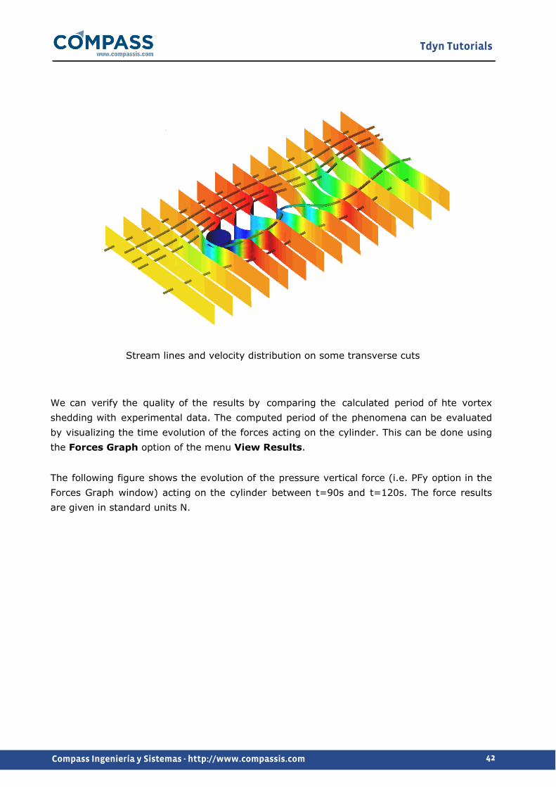
Stream lines and velocity distribution on some transverse cuts

We can verify the quality of the results by comparing the calculated period of hte vortex shedding with experimental data. The computed period of the phenomena can be evaluated by visualizing the time evolution of the forces acting on the cylinder. This can be done using the Forces Graph option of the menu View Results.

The following figure shows the evolution of the pressure vertical force (i.e. PFy option in the Forces Graph window) acting on the cylinder between t=90s and t=120s. The force results are given in standard units N.

Tdyn Tutorials


Evolution in time of the pressure vertical force acting on the cylinder

It can be observed that the period of the vortex sheding is about 6 seconds, which agrees quite well with the experimental value T = 5.98 s reported in [13]. The calculated period leads to a Strouhal number Str = 0.16 wich is also very close to the experimental value obtained in [13] and about 6% below the numerical value reported in [14].

5 Advanced tutorials

Tdyn Tutorials


Backward facing step -pag. 57-Heat transfer analysis of a solid -pag. 184-Species advection -pag. 70-ALE Cylinder -pag. 79-Fluid-Solid thermal contact -pag. 84-Analysis of an electric motor -pag. 92-Analysis of a dam break -pag. 100-Compressible flow around a NACA airfoil profile -pag. 107-3D Cavity flow -pag. 115-Laminar flow in a 2D pipe -pag. 125-Turbulent flow in a 2D pipe -pag. 131-Laminar and turbulent flow in a 3D pipe -pag. 139-The Ekman's spiral -pag. 151-The Taylor-Couette flow -pag. 168-Three dimensional flow passing a cylinder -pag. 32-Heat transfer analysis of a 3D solid -pag. 184-Towing analysis of a wigley hull -pag. 190-Wigley hull in head waves -pag. 215-Thermal contact between 2 solids -pag. 225-Fluid-structure interaction -pag. 232-Potential flow with free surface -pag. 249-2D Sloshing test -pag. 263-

Two-dimensional flow passing a cylinder

Introduction

The fourth example of this tutorial analyses a case of two-dimensional flow passing a cylinder in the low Reynolds number range.

We choose a Reynolds number of Re = 100, for which we expect a vortex street in the wake of the cylinder (the well known von Kármán vortex street).

As in the two previous examples the geometry consists of a box that represents the control volume, which contains the body to be studied in this case a circular cylinder.

Tdyn Tutorials


The Reynolds number is calculated as in the cavity flow example. In this case the characteristic length of the problem is given by the diameter D of the cylinder. The complete set of parameters describing the problem are:

D = 1.0 m

v = 1.0 m/s

ρ = 1.0 kg/m3

μ = 1·10-2 kg/m·s

which provide a Reynolds number Re = 100

Start data

For this case, the same kind of problems as in the previous tutorial must be loaded in the Start Data window of the CompassFEM suite.



Pre-processing

Again the geometry for this example is created using the Pre-processor. First we have to create points with the coordinates given in the table below.

Tdyn Tutorials


Points

Nº X coordinate Y coordinate Z coordinate

1 -4.000 -3.500 0.000

2 -4.000 0.000 0.000

3 -4.000 3.500 0.000

4 9.000 3.500 0.000

5 9.000 0.000 0.000

6 9.000 -3.500 0.000

7 0.500 0.000 0.000

8 -0.500 0.000 0.000

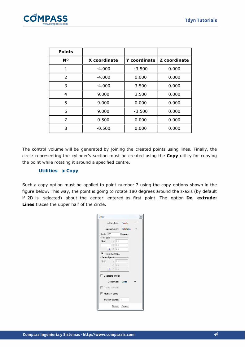
The control volume will be generated by joining the created points using lines. Finally, the circle representing the cylinder's section must be created using the Copy utility for copying the point while rotating it around a specified centre.

Utilities Copy

Such a copy option must be applied to point number 7 using the copy options shown in the figure below. This way, the point is going to rotate 180 degrees around the z-axis (by default if 2D is selected) about the center entered as first point. The option Do extrude: Lines traces the upper half of the circle.

Tdyn Tutorials


In order to draw the rest of the circle it is necessary to apply the same action to point No 8 just changing the value of the rotation angle to θ=-180

Initial data

Initial data for the analysis can be entered in the following section of the CompassFEM data tree. In this case, only the Initial Velocity X Field must be fixed to 1.0 m/s

Conds. & Init. Data Fluid Flow Initial and Field Velocity X Field

This initial data option will be further used in order to fix the velocity on the inlet edge of the control volume to the especified value.

Boundary conditions

Once the geometry of the control domain has been defined, we can proceed to set up the boundary conditions of the problem (access the conditions menu as shown in example 1). The conditions to be applied in this tutorial are:

a) Velocity Field [line]


This condition is used to fix the velocity on a line to the value given in the following section of the data tree.

Conditions & Initial Data Initial and Field Data

Velocity X Field and Velocity Y Field can define a space-time-variable dependant function and thus the Velocity Field condition can be used to specify a variable inflow. In order to do this, the corresponding Fix Field flag must be activated. It is also possible to fix the Velocity (during the run) to the initial value of the function given in the above mentioned entries. In order to do this, the corresponding Fix Initial flag should be marked.

Now, this condition will be assigned to the inflow and lateral lines of the channel (see figure below). In our case, all the velocity components have to be fixed for the inflow lines (i.e. mark Fix Field X and Fix Field Y) and only the vertical component for the lateral lines (i.e. mark Fix Field Y). Then, the corresponding components will be fixed to their initial values.

Tdyn Tutorials


b) Fix Pressure [Line]

As mentioned in example 1, in order to solve the problem, the pressure must be fixed at least in one point of the control domain (taken as reference). Here we will apply the corresponding condition to the outflow lines of the domain.


By imposing this condition, the value of the dynamic pressure defined in the corresponding Material (Fluid) (p = p-ρgz in our case) will be then assigned to this line.

Materials

Physical properties of the materials used in the problem are defined in the section following section of the CompassFEM Data tree.


Some predefined materials already exist, while new material properties can be also defined if needed.

For the present tutorial, only Fluid Flow properties are necessary for the fluid material which must be assigned to the only existing surface of the model (that defining the control volume of the present 2D case). This assignment is done using the following option

Materials Fluid

Tdyn Tutorials


In this case, Density and Viscosity of the fluid are fixed to 1.0 Kg/m3 and 1.0e-2 Kg/m·s respectively.

For every parameter, the respective units have to be verified, and changed if necessary (in our example, all the values are given in default units).

Boundaries

Fluid Wall/Bodies

In this case only one fluid Wall condition is necessary. V FixWall type will be assigned to the boundary type of the wall.

This condition has to be assigned to the lines that define the cylinder geometry.

Problem data

Other problem data must be entered by using the following options.



For this example, only the Fluid Flow must be solved by using the following parameters:



Max. iterations 3

Initial steps 0


Output Step 10

Output Start 600

Remark: parameter OutPut Start is used to define when the program will begin to write the results. In this case, it has been fixed to 600 in order to reduce the size of the results file.

A brief summary of the boundary conditions, boundary definitions and material properties that have been applied to the control domain is given in what follows:

Tdyn Tutorials



Velocity Field (line) Fix X Velocity, Fix Y Velocity

Lines 4, 6

Velocity Field (line) Fix Y Velocity Lines 1, 3

Fluid Body - Lines 9, 10

Fluid - Surfaces 1, 2

Pressure Field (line) - Lines 2, 7

Mesh generation


Size assignment

The mesh should be finner in the vicinity of the cylinder. Therefore we will assign a size of 0.03 to the cylinder lines and points and a size of 0.1 to the symmetry line. The global size of the mesh is chosen to be 0.3, and an Unstructured size transition (Meshing Preferences window) of 0.5 will be used. These values have been chosen by a 'trial and error'-procedure, i.e. first some approximate values are chosen, out of experience and/or practical considerations. With these parameters a mesh is generated. If the obtained number of nodes is too large or too small, the parameters need to be adjusted correspondingly. Finally, we will obtain an unstructured mesh consisting of 2160 nodes and 4464 triangle elements.

Calculate

Tdyn Tutorials



Post-processing


The results shown below correspond to the last time step (t = 120 s) of the simulation.

Tdyn Tutorials


The evolution in time of any parameter can be captured and visualised by means of the Animate utility of GiD (accessible through the Window main menu or by pressing Ctrl+m). Selecting Save MPEG option in the Animate window allows to save the corresponding animation in MPEG format. In order to save disk space, it is advisable to reduce the GiD window size to the essential details, since the whole interior of the GiD main window will be saved. This can result in very large files. To prevent this, the empty space around the area of interest should be also minimised.

Time evolution of the velocity module is shown in the following figures. From left to right and from top to bottom, each caption corresponds to t=60 s,t=62 s, t=64 s, t=66 s, t=68 s, t=70 s, t=72 s, t=74 s, t=76 s and t=78 s.

Tdyn Tutorials


Remarks

a) We can observe that the perturbances induced by the cylinder in the velocity and pressure fields reach the boundaries of the control volume. Normally this should be avoided by choosing a larger control volume, as the boundary conditions can perturb the solution. This has not been possible here because of the limits of the academic version of Tdyn (a larger domain would imply a larger mesh). Nevertheless quite accurate results are obtained.

b) The quality of the results can be verified by comparing the calculated period of the vortex shedding with experimental and other numerical results [12, 14]. The periodical character of the vortex shedding phenomenon is described by the Strouhal number, given by

Str = f·D/v∞

being f the frequency of the vortex shedding, D the diameter of the cylinder, and v∞ the

free-stream velocity. The computed period can be evaluated in many ways as for instance through the evolution of a variable at a point behind the cylinder, or through the evolution of the net force over it. Nevertheless, we will first calculate the period using another GiD facility, i.e the Graph menu option.

Tdyn Tutorials


We can access the Graph point analysis utility through the following menu sequence

View results->Graphs->Point evolution

and select the physical quantity we want to analyse - here the x-component of the velocity - and select the point we want to analyse using the join option. In this case, we should select a lateral point in the wake of the cylinder. In a more central point, the x-component of the velocity would oscillate at twice the frequency, as it changes every time a vortex is shed. The lateral points, however, are only affected by vortices shed on the respective side of the cylinder. The point should also be far enough from the boundaries, as these can also affect the velocity evolution.

Tdyn Tutorials


As can be seen the resolution of the graph is not good enough since just one point is drawn every 10 time steps (every second) as fixed in the problem type window. However the period can be estimated quite accurately to be T = 6.0 s.

It is also possible to calculate the period of the phenomenon by visualising the time evolution of the forces acting on the cylinder. This can be done using the Forces Graph option of the Utilities menu. Through this option, different components of forces and momentum can be drawn. They are listed in the following table (all values given in standard unit kg, m and s):

PFx : Ox pressure force component on the boundary

PFy : Oy pressure force component on the boundary

PFz : Oz pressure force component on the boundary

MFx : Ox pressure momentum component on the boundary (calculated respect to the origin)

MFy : Oy pressure momentum component on the boundary (calculated respect to the origin)

MFz : Oz pressure momentum component on the boundary (calculated respect to the origin)

VFx : Ox viscous force component on the boundary (calculated by integrating viscous stresses on surface)

VFy : Oy viscous force component on the boundary (calculated by integrating viscous stresses on surface)

VFz : Oz viscous force component on the boundary (calculated by integrating viscous stresses on surface)

MVFx : Ox viscous momentum component on the boundary (calculated respect to the origin)

MVFy : Oy viscous momentum component on the boundary (calculated respect to the origin)

Tdyn Tutorials


MVFz : Oz viscous momentum component on the boundary (calculated respect to the origin)

The following figure shows the evolution of the pressure vertical force (PFy option) on the cylinder. It can be observed that the oscillatory phenomena is completely developed after 68 seconds and that the period of the process is about 6.0 seconds, as mentioned above. This is to be compared with the experimental value of T = 5.98 s reported in [13]. The calculated period leads to a Strouhal number of Str = 0.167 which is very close to the experimental value obtained in [13] and about 5% below the numerical value reported in [14].

Tdyn Tutorials


Backward facing step

Introduction

This example is a two-dimensional study of a fluid flow within a channel with a backward-facing step.

The flow pattern will be again calculated using the incompressible Navier-Stokes equations for a Reynolds number Re = 250, which for this problem lies in the laminar range (the transitional range lies between 1200 < Re < 6600).

The geometry basically consists on a box representing the channel with a step at the channel bottom.

The Reynolds number is defined here as: Re = 2vmaxDρ/3μ being the characteristic length D

the height of the inlet channel.

The factor 2/3 derives from the assumption of a parabolic velocity profile in the inlet section with vmax being the maximum velocity attained in this section.

The value of the Reynolds number is obtained from the choice of the following parameters:

D = 1.5 m

vmax = 0.5 m/s

ρ = 1000 kg/m3

μ = 2 kg/m·s

According to the equation presented above the following value is obtained for the Reynolds number Re = 250

Start data

Tdyn Tutorials


In this case, it is necessary to load the following types of problem in the Start Data window of the CompassFEM suite.



Pre-processing

The geometry for this example will be created just as in the Cavity Flow tutorial using the Preprocessor module. The geometry will again resemble a box, but with a step at its bottom surface.

By entering the points with the co-ordinates given below, then joining them into lines and finally creating the control surface, we will obtain the geometry that can be checked in the Figure shown in the introduction section. For details on creating the geometry, please refer to the Pre-processing section of Tutorial 1.

Point number X Coordinate Y Coordinate

1 0.000000 0.500000

2 4.000000 0.500000

3 4.000000 0.000000

4 20.00000 0.000000

5 20.00000 2.000000

6 0.000000 2.000000

Initial data

The initial values of the velocity and other variables can be specified in the following section section of the CompassFEM data tree.

Conditions & Initial Data Initial and Conditional Data Initial and Field Data

In the present case, a function that defines a parabolic profile must be inserted in the Velocity X Field:


Tdyn Tutorials


Such a parabolic velocity profile must be applied at the inflow of the channel.

Boundary conditions

Once the geometry of the control domain has been defined and the initial conditions have been specified, we can proceed to set up the boundary conditions of the problem. The conditions to be applied in this tutorial are:

a) Velocity Field [lines]

b) Fixed Velocity [lines]

c) Pressure Field [lines]

a) Velocity Field [lines]

This condition is used to impose the velocity on a line equal to the value given in the Initial and Field data section.

Any of the fields can be a time dependent function and in particular the Velocity Field condition can be used to specify a variable inflow. In order to do this, the corresponding Fix Field flags have to be marked as shown in the figure below.


Tdyn Tutorials


It is also possible to fix the Velocity (during the run) to the initial value of the function given in the corresponding Initial and Field data section. In order to do this, the corresponding Fix Initial flag should be marked.

In this example the Fix Field X and Y conditions are going to be assigned to the inflow line of the channel. Coincidentally, this happens to be similar as the Fixed Velocity condition used in the cavity flow example; the difference here is that the fluid now enters through this surface, whereas in the previous case it was only tangent to the surface to which the condition was assigned.

Remark: the above condition will not work if the Start-up control option is activated in the Fluid Dyn. & Multiphy. Data->Analysis section. Then this option must be switched off.

b) Fix Velocity [line]

As explained in the example 1, this condition is used to impose the velocity on a line. For this example this condition is going to be assigned to the step line. Both velocity components will be set to 0.0 m/s. Then, all the velocity components have to be fixed to the specified value (i.e. Fix X Velocity and Fix Y Velocity must be activated).


Tdyn Tutorials


c) Pressure Field [line]

As explained in example 1, in order to solve the problem, the pressure must be fixed at least in one point of the control domain (taken as reference). Here we will apply the Pressure Field condition to the outflow line of the domain. The value of the dynamic pressure specified in the Initial and Field data section (p = po-ρgz in our case) will be further assigned to the outflow

line. In this case, we will assume p = 0.

Conditions & Initial Data Fluid Flow Pressure Field

Materials

Physical properties of the materials used in the problem are defined in the following section of the CompassFEM Data tree.


Some predefined materials already exist, while new material properties can be also defined if needed. In the presnet case, only Fluid Flow properties are necessary for the fluid material that has to be assigned to the only existing surface of the model (which defines the control volume of the present 2D case). This assignment is done through the following section of the data tree.

Materials Fluid

Different material assignements can be checked at any time by accessing the Draw

Tdyn Tutorials


groups options of the corresponding group within the

Materials Fluid

section of the data tree.

In this case, Density and Viscosity of the fluid are fixed to 1000.0 Kg/m3 and 2.0 Kg/m·s respectively.

Boundaries

Fluid Wall/Bodies

In this tutorial, two different kind of boundaries will be applied to different parts of the model. Hence, two new wall conditions must be defined in the following section of the data tree, and they have to be further applied to the corresponding groups of entities in the model.

Conditions & Initial Data Fluid Flow Wall/Bodies

In this case the values of both fluid boundaries correspond to those of a V FixWall boundary type. The first one of the boundaries must be applied to the upper and bottom lines of the main channel, while the second one has to be assigned to the lines that define the step. Note that in the present case these boundaries could actually have been imposed by using only one boundary or by means of the line condition.


However the above definition can be used for different problems.

Problem data

Other problem data must be entered in the section.


For this example, only the Fluid Flow must be solved by using the following parameters:

Number of steps 300


Max. iterations 3

Initial steps 25


A brief summary of the boundary conditions, boundary definitions and material properties

Tdyn Tutorials


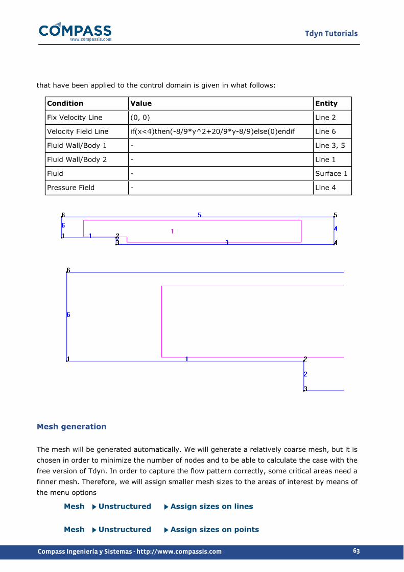
that have been applied to the control domain is given in what follows:


Fix Velocity Line (0, 0) Line 2

Velocity Field Line if(x<4)then(-8/9*y^2+20/9*y-8/9)else(0)endif Line 6

Fluid Wall/Body 1 - Line 3, 5

Fluid Wall/Body 2 - Line 1

Fluid - Surface 1

Pressure Field - Line 4

Mesh generation

The mesh will be generated automatically. We will generate a relatively coarse mesh, but it is chosen in order to minimize the number of nodes and to be able to calculate the case with the free version of Tdyn. In order to capture the flow pattern correctly, some critical areas need a finner mesh. Therefore, we will assign smaller mesh sizes to the areas of interest by means of the menu options

Mesh Unstructured Assign sizes on lines

Mesh Unstructured Assign sizes on points

Tdyn Tutorials


In particular, we will assign the size 0.03 to the step line. The same element size will be assigned to the edge points of the step and a size of 0.06 to the inflow line. Finally, the Unstructured size transition will be set to 0.4 and the Elements general size to 0.2.

The outcome of the mesh generation process is the unstructured mesh shown below, consisting of almost 1700 nodes and 3000 elements.

The number of mesh nodes and elements can be checked through the menu option

Utilities Status

If the size of the obtained mesh results to be significantly different from the size report herein, please make sure that the following option is set to None (especially if the nodes limit of Tdyn's academic version is exceeded).

Utilities Preferences Meshing Automatic correct sizes

(Note that it is usually extremely convenient for beginners to activate the automatic correct sizes option).

Calculate

The calculation process will be started from GiD through the Calculate menu, exactly as described in the previous example.

The results file ProblemName.flavia.res is the file that will be loaded when pressing the Postprocess button.

Post-processing

When the calculations are finished, the message Process '...', started on ... has

Tdyn Tutorials


finished is displayed. Then we can proceed to visualizing the results by pressing the Postprocess button (therefore the problem must still be loaded; should this not be the case, we first have to open the problem file again).

As the post-processing options to be used are the same as in the previous tutorials, they will not be described in detail here again. For further information please refer to the Post-processing chapter of tutorial 1 and to the Pre/Postprocessor user manual or online help.

The results given below correspond to the last time step t=150 s.

Tdyn Tutorials


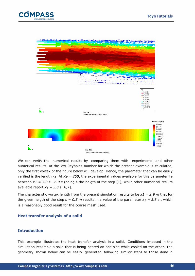
We can verify the numerical results by comparing them with experimental and other numerical results. At the low Reynolds number for which the present example is calculated, only the first vortex of the figure below will develop. Hence, the parameter that can be easily verified is the length x1. At Re = 250, the experimental values available for this parameter lie

between x1 = 5.0 s - 6.0 s (being s the heigth of the step [1], while other numerical results available report x1 = 5.0 s [6,7].

The characteristic vortex length from the present simulation results to be x1 = 2.9 m that for the given heigth of the step s = 0.5 m results in a value of the parameter x1 = 5.8 s , which

is a reasonably good result for the coarse mesh used.

Heat transfer analysis of a solid

Introduction

This example illustrates the heat transfer analysis in a solid. Conditions imposed in the simulation resemble a solid that is being heated on one side while cooled on the other. The geometry shown below can be easily generated following similar steps to those done in

Tdyn Tutorials


previous examples. Geometric data in the figure below is given in cm.

Start data


2D Plane Solid Heat Transfer


Pre-processing

The geometry used in this tutorial is shown in the figure of the introduction section.

Boundary conditions

Once the geometry of the control domain has been defined, we can proceed to set up the boundary conditions of the problem (access the conditions menu as shown in example 1). The only condition to be applied in this example is a Fixed Temperature [line] condition (see example 2 for further information).


First, temperature must be fixed to T=2ºC at top, bottom and right edges of the solid block at the right side. Finally, temperature must be fixed to T=23ºC at the left edge of the solid block at the left side of the model.

Tdyn Tutorials


Materials

Physical properties of the materials used in the problem are defined in the materials section of the CompassFEM Data tree.


Some predefined materials already exist, while new material properties can be also defined if needed. For the present case, a predefined solid with the properties of aluminium will be used. Since only the Solid Heat Transfer module is active for the present analysis, just the thermal properties of the selected material appear within the corresponding entry of the data tree. For every parameter, the corresponding units have to be verified, and changed if necessary (in our example, all the values are given in default units).

The material above defined must be assigned to the only existing surface of the model (that defining the control volume of the present 2D case).

Materials Solid

Problem data

Other problem data must be entered in order to complete the analysis setup. For this example, only the Solid Heat Transfer problem must be solved by using the following parameters:



Number of steps 100


Max. iterations 3

Initial steps 0


Output Step 25

Output Start 1

Mesh generation

The mesh will be again generated automatically by using a default element size of 0.1. The

Tdyn Tutorials


outcome of the mesh generation process is an unstructured mesh consisting of 997 nodes and 1830 triangle elements:

Calculate


Post-processing


The results shown below correspond to temperature distribution obtained for the last time step (t = 25 s).

Temperature distribution

Tdyn Tutorials


Species advection

Introduction

The next example of this tutorials manual analyses a case of transport of two species in a squared domain. The geometry consists of a box that represents the control volume, which contains a circle, where there is an initial concentration of species. Transport of species is produced in this case by the advection in a fluid that is moving with a constant velocity given by the vector (1.0,1.0,0.0) m/s.

Start data


2D Plane Fluid Species Advection


Since in this particular example the advection velocity is constant and fixed on the entire domain, the fluid flow problem does not need to be solved so that Fluif Flow modul is not loaded on the Start Data window (see Initial data -pag. 71- for further deatils).

Tdyn Tutorials


Pre-processing

Again, the geometry for this tutorial is created using the GID Pre-processor.

First we have to create the points with the coordinates given below, and then join them into lines (the edges of the control volume).

No X coordinate Y coordinate Z coordinate

1. 0.000000 0.000000 0.000000

2. 3.000000 0.000000 0.000000

3. 3.000000 3.000000 0.000000

4. 0.000000 3.000000 0.000000

Then we create the circle representing the source of species using the GID pre-processor utilities as follows:

Geometry Create Object Circle

The circle must have a radius of 0.25m and its centre is at the point (1.0, 1.0, 0.0).

Finally the external surface of the geometry can be created, by selecting all existing edges. The outcome is the final geometry shown in the introduction section (Species advection -pag. 70-).

Initial data

Initial and field data may be specified in the following section of the data tree:

Conditions & Initial Data

The values entered in this section could be further used to impose boundary conditions to selected contours of the model. Nevertheless, in this particular example the velocity is constant everywhere and the fluid flow problem does not need to be solved actually. Consequently, no velocity field conditions need to be specified and a constant velocity value is just needed to setup the advection problem. Hence, X and Y components of the initial velocity are set to 1.0 m/s and the velocity components are automatically fixed on the entire domain to this initial value.

Species initial data is no longer updated in the Conditions and Initial Data section of the data tree. Instead of that, initial and conditional data must be specified individually for each

Tdyn Tutorials


one of the species that must be previously created and defined in the following section of the CompassFEM data tree.

Materials Edit Species

See Materials -pag. 72- for additional information.

Materials

Since boundary conditions for species advection problems must be specified for each one of the species under analysis, it is necessary to create and define those species before applying the corresponding boundary conditions. This is done as follows in the Materials section.

Fluid materials definition

Two different materials (Generic_Fluid1 and Generic_Fluid2) with the same physical properties must be created for the present analysis. Since the fluid flow problem is not going to be solved, the actual physical properties of the fluid are not important. In fact, this materials are just a vehicle to facilitate the proper assignement of initial conditions and/or conditional data concerning the concentration variable of each one of the species under analysis. Hence, Generic_Fluid1 and Generic_Fluid2 are created and assigned to the "External region" group (external squared surface) and to the "Source region" group (internal circular surface) respectively (see picture below).

As mentioned above, this materials assignment provides an easy way to specify an initial concentration value of 1 C to the inner surface of the model, while the rest of the squared domain has a zero initial concentration per specie.

Tdyn Tutorials


Species definition

Although a default specie exists on the data tree if the species advection problem has been activated, an arbitrary number of additional species can be created and defined in the following section of the data tree.

Materials Edit Species

In the present analysis, two different species will be studied. Hence, another additional specie must be created as shown in the figure below.

The species advection problem is automatically solved over the entire domain for all defined species. Advection and diffusion coefficients need to be updated separately for each one of the species under analysis. In this particular example, the difusion of Specie2 will be considered to double that of Specie1 (see figure below).

Tdyn Tutorials


Finally, initial and conditional data can be easily fixed for both species by using the vehicle materials that where define above and assigned to the two different regions of the domain. In particular, initial concentration of both species will be fixed to 1 for those points inside of the inner circular region and set to 0 outside of it. This can be done specifying the following function in the concentration field.

if(group(Source region))then(1)else(0)endif

Note that, within the function used to specify the initial concentration, the name of the group

Tdyn Tutorials


(Source region in this case) must be used instead of the name of the corresponding material (Generic_Fluid2).

Boundary conditions

Fix Concentration

Once all species under analysis have been created and their properties defined boundary conditions can be specified at particular contours of the model for each one of the species. In our particular case, the concentration of both species will be fixed to 0 for the left and bottom edges of the control domain. This is done through the following option of the CompassFEM data tree.

Conditions & Initial Data Species Advection Fix Concentration

Note again that the value of the concentration must be prescribed separately for each specie at all the prescribed boundaries.

Problem data

Once the boundary conditions have been assigned and the materials have been defined, we have to specify the other parameters of the problem. The values listed next have to be entered in the Problem, Analysis, Results and Fluid Solver pages of the Fluid Dyn. & Multi-phy. Data section of the data tree.

Solve Species Advection 1

Tdyn Tutorials


Number of Steps 400

Time Increment 0.005

Max Iterations 1

Initial Steps 0

Output Step 40

Time Integration Crank Nicolson

Remark: in this problem, we have changed the time integration scheme in order to increase the accuracy of the results. This is done, by selecting Crank_Nicolson in the Time Integration field. This way, the time integration scheme used in the solution process of the fluid problem will be an implicit 2nd order scheme. Note that in some cases, the use of a 2nd order scheme may create some instability in the solution process.

Mesh generation

As usual we will generate a 2D mesh by means of GiD's meshing capabilities. We will use a mesh composed of triangles inside the circular surface and quadrilaterals for the rest of the domain. In order to do it, we have to assign a quadrilateral element type to the external surface of the model geometry.

Mesh Element type Quadrilateral

To generate the mesh, the global size of the elements is chosen to be 0.025, and an unstructured size transition of 0.5 is used.

With these parameters a mesh is generated which contains about 17000 nodes, with 1000 triangular elements and 16400 quadrilateral elements.

Calculate


Post-processing

When the analysis is completed and the message Process '...' started on ... has finished. has been displayed, we can proceed to visualise the results by pressing Postprocess. For details on the results visualisation not explained here, please refer to the Post-processing chapter of the previous examples and to the Postprocess reference manual.

Tdyn Tutorials


Below, the results corresponding to the time evolution of the concentration of the two species are shown. The effect of the different diffusion coefficient may be observed.

t = 0.4 s t = 0.4 s

t = 0.8 s t = 0.8 s

t = 1.2 s t = 1.2 s

Tdyn Tutorials


t = 1.6 s t = 1.6 s

t = 2.0 s t = 2.0 s

Tdyn Tutorials


ALE Cylinder

Introduction

This tutorial simulates a cylinder moving with uniform velocity within a fluid at rest. The resulting global Reynolds number is Re=100. Actually, this problem is similar to that shown in Two-dimensional flow passing a cylinder -pag. 44-, but in this case what is actually simulated is a moving object in a fluid at rest. This kind of simulations requiere the mesh to be updated every time step due to the movement of the body. In order to solve this kind of problems it is possible to use those tools available in the ALEMESH module of the CompassFEM suite.

The starting point for the present problem will be the file used to analyse the problem presented in section Two-dimensional flow passing a cylinder -pag. 44-. We will only detail here the necessary steps to update the previous example with the new data.

Start data

For this case, an additional type of problem must be loaded in the Start Data window of the CompassFEM suite to make available the mesh deformation capabilities of the CompassFEM suite. Hence the following are the type of problems required for the present simulation:

2D Plane Flow in Fluids Mesh Deformation


Pre-processing

The geometry for this example is exactlly the same as in Two-dimensional flow passing a cylinder -pag. 44-. Hence, the previous tutorial must be loaded and only the Start Data must be updated as indicated in the preceding section Start data -pag. 79-.

Initial data

Initial data for the analysis must be updated. In particular, the Initial Velocity X Field must be fixed to 0.0 m/s.


Tdyn Tutorials


This way, the Velocity Field condition that will be further used in order to fix the velocity on the inlet edge of the control volume willl have no effect on the fluid.


Boundary conditions

The Wall/Body condition applied to the cylinder walls in section Boundary conditions -pag. 47- will remain the same but its motion properties must be updated in order to specify the movement of the cylinder.

Conditions & Initial Data Fluid Flow Wall/Bodies ... Motions

The corresponding parameters must be fixed as shown in the figure below.

When any Displacement field is defined as Fixed, the corresponding displacement values field becomes available and can be used to define the displacement of the Fluid Body every time step. In our case a displacement of -1.0*t means that the cylinder is moving forward with a velocity of 1.0 m/s.

Boundaries

Fluid Wall/Bodies

Tdyn Tutorials


wall type tab properties of the Wall/Body entity assigned to the cylinder does not need to be updated. Hence, V FixWall type will remain applied to the walls of the cylinder as in the case of the parent tutorial (see Boundaries -pag. 49-).

Modules data

Specific parameters must be entered in the Modules Data section of the data tree. For the present case, it is necessary to especify new data in the Mesh Deformation page as shown in figure below. By selecting the option ByBodies in the Fluid Mesh Deformation entry, the calculation will update mesh data following the movement of the previously defined Fluid Body (cylinder).

Modules Data Mesh Deformation

Problem data

The only necessary update to the Problem Data is the activation of the mesh deformation type of problem in order for that to be actually solved (see figure below). Note that this type of problem is automatically activated when the Mesh Deformation option is added to the selected type of analysis in the Start Data window.

Tdyn Tutorials


Calculate

As in previous tutorials, the analysis process will be started from within GiD through the Calculate menu.

Post-processing


In this example, the obtained results will be very similar to those shown in the Post-processing -pag. 51- section of the Two-dimensional flow passing a cylinder -pag. 44- tutorial. However we can see significant differences if we look at velocity results. Differences in the velocity fields are due to the fact that in the present example the external fluid is at rest, being perturbed by the movement of the cylinder. The evolution of the velocity field is shown in the set of figures below.

Tdyn Tutorials


t = 60.0 s t = 62.0 s

t = 64.0 s t = 66.0 s

t = 68.0 s t = 70.0 s

t = 72.0 s t = 74.0 s

t = 76.0 s t = 78.0 s

Tdyn Tutorials


Fluid-Solid thermal contact

Introduction

This tutorial studies the flow pattern that appears in a square cavity when it is heated on one side, in contact with a hot solid.

Actually, this example is based on the Example 2 - Cavity flow, heat transfer tutorial.

Start data


2D Plane Flow in Fluids Fluid Heat Transfer Solid Heat Transfer


Pre-processing

The geometry of the present model simply consists of two squares, representing a cavity filled with a fluid, in contact with a solid block. The easiest way to generate the complete geometry of the model, is by duplicating the existing square of the Example 2 - Cavity flow, heat transfer tutorial. To this aim, load the Cavity flow, heat transfer model and copy the existing surface using the options shown in the figure below. With this options, an automatic translation of the new entity will be performed along the X-direction so that both squared-shape blocks will remain in contact.

Tdyn Tutorials


Copy window

When doing the copy of the original square, do not forget to select the option Duplicate entities in the Copy window. This way, the edge that defines the contact boundary will be duplicated.

Boundary conditions

Once we have defined the geometry of the control volume, it is necessary to set the boundary conditions of the problem.

Tdyn Tutorials


a) Fix Pressure [point]


In most cases, it is recommended to fix the pressure at least in one point of the control domain (taken as reference). If this condition is not applied, automatic corrections are applied during the calculation and the solution of the problem is equally achieved most of the times. In this case, the pressure reference point will be applied to the bottom right corner of the model geometry.

b) Fix Temperature [line]


The Fix Temperature [line] condition is used to fix the temperature on a given edge of the geometry. In this example two distinct conditions will be assigned to the left line of the geometry with the value 100oC and to the right line with the value 0oC respectively.

Materials

Materials used in the problem are created and/or defined in the Materials section of the data tree. Some predefined materials already exist, while new material properties can be also defined if needed. In the present case, fluid properties must be assigned to the surface on the right, while solid properties are assigned to the surface on the left.

Materials (Fluid)

Both, Fluid Flow and Heat Transfer properties need to be specified for the fluid domain. To this aim, the existing set of Physical Properties Generic_Fluid1 may be updated. Default values will be preserved for Fluid Flow properties.

Materials Physical Properties Generic Fluid Generic_Fluid1 Fluid Flow

On the contrary, heat transfer properties are going to be updated by setting the Specific Heat to 10 J/kgºC and redefining the flotability value to be 0.1*Tm.

Materials Physical Properties Generic Fluid Generic_Fluid1 Heat Transfer

Finally, the updated set of properties Generic_Fluid1 is assigned to the model surface on the right side.

Materials Fluid

Materials (Solid)

Tdyn Tutorials


In the case of the solid, only Heat Transfer properties are relevant for the present analysis. By edditing the allready existing set of Physical Properties named Generic_Solid1, it is only necessary to update the Specific Heat value to 10 J/kgºC.

Materials Physical Properties Generic Fluid Generic_Solid1 Heat Transfer

Finally, the updated set of properties Generic_Solid1 is assigned to the model surface on the left side.

Materials Solid

Boundaries

Next, boundary properties need to be assigned to the corresponding contours of the model.

Fluid Wall/Bodies

In our case a Fluid Wall of V FixWall type must be assigned to the contour lines of the fluid cavity. This is readillly done through the following option of the data tree.


Contacts

Next, a contact between the solid and the fluid should be defined.

Fluid-Solid contact (FSContact):

FSContact boundaries identify a contact with continuity of the corresponding fields between solid and fluid domains. We will use this boundary to define the continuity of the temperature field through the two central (contact) lines. The FSContact boundary can be applied in the Contacts section of the CompassFEM data tree.

Contacts Fluid-Solid Contacts

Analogously, FFContacts can be used to create a contact with continuity in the selected fields between two fluid domains and SSContacts to create a contact with continuity in the selected fields between two solid domains.

In the present case, only temperature field continuity through the contact surface must be ensured, since the fluid flow problem is not solved within the solid domain. Hence, only heat transfer contact definition must be updated as shown in the figure below.

Tdyn Tutorials


Contacts window (temperature field continuity)

Finally, contact properties can be assigned to the central (contacting) lines of the model geometry as shown in the following figure:

Contacts assgienment window

Tdyn Tutorials


Contact group assignement

Tdyn Tutorials


Problem data

Once the boundary conditions have been assigned and the materials have been defined, we have to specify the other parameters of the problem. The values listed next have to be entered in the corresponding sections of the data tree.

Fluid Dynamics & Multi-Physics Data Solve Fluid

Solve Fluid Flow 1 (YES)

Solve Heat Transfer 1 (YES)

Fluid Dynamics & Multi-Physics Data Solve Solid

Solve Fluid Flow 0 (NO)



Number of Steps 100


MAx iterations 1

Initial steps 0

Start-up control Time

Mesh generation

The mesh to be used in this example will be generated by assigning element sizes of 0.03 and 0.1 to the fluid and solid surfaces respectively.

Calculate


Post-processing

Tdyn Tutorials



The results given below correspond to the last time step t = 10s.

Temperature distribution (contour fill)

Velocity field distribution (contour fill)

Tdyn Tutorials


Analysis of an electric motor

Introduction

This example studies the 2D static magnetic field due to the stator winding in a two-pole electric motor.The present 2D analysis of the motor assumes that the variation of the magnetic field in the z-direction is negligible, and therefore the magnetic potential equation can be simplified as shown below.

The magnetic potential is governed by the equation:

∂/∂x(1/m ∂Az/∂x)+∂/∂y(1/m ∂Az/∂y)+Jz = 0

Where Az is the magnetic potencial, Jz is the current density and m is the magnetic

permeability.

For this problem we will use the URSOLVER module capabilities of the CompassFEM suite. This module provides pertinent calculation tools for the solution of partial diferential equations (PDE) defined by the user. The new variables defined in this module (noted internally as ph1, ph2, ph3, being ph1 the solution of the first defined equation, ph2 the solution of the second, etc) can be coupled with any other variable of the problem.

In terms of the standard notation used in the URSOLVER module, above equation can be re-written as:

∂/∂x(f2xx ∂ph1/∂x)+∂/∂y(f2yy ∂ph1/∂y)+f4 = 0

The geometry of the motor under analysis is shown in the following figure:

Tdyn Tutorials


Start data


2D Plane Solid Generic PDE's Solver


Pre-processing

The geometry used in this example is shown in the Introduction section (Analysis of an electric motor -pag. 92-). It represents just a quarter of the total motor model, since the symmetries of the problem have been allready taken into account.

Boundary conditions

Once we have defined the geometry of the control volume, it is necessary to set the boundary conditions of the problem. This process is carried out in the Conds. & Init. Data section of the data tree. In this case, the only boundary condition to be applied implies fixing the value of the user defined variable (URSOLVER phi) on the left line and the external border of the geometry.

Conditions & Initial Data PDEs Solver Fix Variable

Tdyn Tutorials


The value to which the variable must be fixed is 0 as shown in the figure below.

Since only one variable will be used in the present problem, the preexisting variable named Variable1, will be used for the assignment. The corresponding properties of this variable will be further edited during materials definition (see section Materials -pag. 94-).

Materials

PDEs Variables

Materials used in the problem are defined in the Materials->Solid section of the data tree. Nevertheless, the first required step, previous to materials definition and assignment, is the creation of the magnetic potential variable. In order to do it, open the Materials->Edit PDEs Variables and rename the existing variable from Variable1 to Potential.

Remark: After renaming the variable, such a change is not automatically updated in the Conds. & Init Data section of the data tree. Since we have already applied in the previous section a Fix Variable boundary condition concerning Variable1, it is important to update this boundary condition container as shown in the figure below.

Tdyn Tutorials


Updating the Fix Variable boundary condition

Each defined user variable will be solved for all existing materials within the model. Hence, the physical properties that determine the behavior of a given variable must be defined as a function of the existing materials. In the present case, only solid properties need to be defined. This is done in the Materials -> Edit PDEs Variables -> <Var_name> -> Solid Props. section of the data tree (see figure below). Remember that in our case <Var_name> was choosen to be Potential.

Tdyn Tutorials


As you can see in the previous figure, a total of 4 coeficients (i.e. f1, f2, f3, f4) need to be defined as a function of the various materials used in the model. Since the present analysis concerns a static problem, no time evolution exists so that f1 equals 0 for all materials. f3 is also 0 while f2 is an homogeneous diagonal matrix whose diagonal terms depend on the material at hand but also on the evolution of the potential variable itself. f2 coefficient can be simply especified by using the following function within the function editor window of the corresponding Var.Definition field:

Finally, f4 can be especified by using the following function in the correspo0nding Var.Definition field:

if(mat(Coil))then(1.0)else(0.0)endif

If necessary, it is possible to create additional PDEs by creating new variables. This is achieved by right-clicking on the Materials->Edit PDEs Variables and apply the Create New Variable option.

Materials (Solid)

Once the properties of the PDE variable have been defined, all materials must be assigned to the corresponding domains of the geometry. In the present case, 4 different materials need to be defined and assigned as indicated in the figure below:

Tdyn Tutorials


Problem data

Once the boundary conditions have been assigned and the materials have been defined, we have to specify the other parameters of the problem. The values listed next have to be entered in the Problem and Analysis pages of the Fluid Dyn. & Multi-phy. Data section of the data tree.

Problem->Solve Solid

Solve PDEs problems 1 (YES)

Analysis

Number of steps 1

Time increment infinite

Max. iterations 3

Initial steps 0

Start-up control None

Nodal assembling algorithm is defined as default setting in Tdyn. This algorithm is faster and more accurate than the standard FEM assembling in most of the cases. However it implies a nodal definition of the material properties and therefore its accuracy is reduced when there is a dramatic change of the properties between two adjacent materials, as in this case. In those cases it is advisable to use the standard elemental assembling instead of the nodal one. This can be modified by selecting the General Data -> Algorithm -> Solid Assemb. Type:

Tdyn Tutorials


Elemental Assembling option in the data tree.

Mesh generation

The mesh to be used in this example will be generated by assigning a maximum element size of 0.02 and an unstructured size transition of 0.3. The resulting mesh is shown in the following figure.

Calculate

The calculation process will be started from within GiD through the Calculate menu, exactly as described in the previous examples.

Post-processing


The results given below correspond to the magnetic potential solution of the defined PDE.

Tdyn Tutorials


Contour field results corresponding to the potential variable U

Tdyn Tutorials


Analysis of a dam break (ODD level set)

This example studies the 2D water evolution in a dam break process, and the encounter of the fluid with two obstacles.

Introduction

This example studies the 2D water evolution in a dam break process. It also studies the encounter of the fluid with two obstacles.

For this problem we will use the OddLevelSet capabilities of the Fluid Dynamics & Multi-Physics module of the CompassFEM suite.

Tdyn Tutorials


Start data


2D Plane Flow in fluids ODD level set

See the Start Data section of the Cavity flow problem (tutorial 1) for details on the Start Data Window.

Aditionally, Geometry Units for the present example must be set to cm in the Start Data window.

Pre-processing

The geometry used in this example is shown in the figure of the introduction section of the present tutorial. It represents the dam that will break at the left, and the two obstacles that the fluid will encounter in its evolution.

Initial data

First, it is necessary to specify some initial pressure conditions for the OddLevelSet analysis. In particular, the Pressure Field option must be filled in with the following function:

Tdyn Tutorials


if(mat(Fluid Auto1))then(9.8*(.025-y))else(0)endif

that must be introduced in the corresponding section of the CompassFEM data tree as indicated in what follows.

Conds. & Init. Data Initial and Conditional Data Initial and Field Data Pressure Field

It is also necessary to fill in the option OddLevelSet Field with the following function as indicated in the figure below:

if(mat(Fluid Auto1))then(1)else(0)endif

Conds. & Init. Data Initial and Conditional Data Initial and Field Data OddLevelSetField

Tdyn Tutorials


Note: the name of the argument used inside of the mat function in the expressions above must be coincident with the name of the group to which the actual material is assigned in the Materials section of the data tree, and whose physical properties are specified in the section

Materials Physical properties

It is also important to ensure that the "Initialize ODDLS function" option is set to 0 for the present analysis.

Materials

Physical properties of the materials used in the problem are defined in the corresponding section of the CompassFEM data tree.


For this simulation, it will be necessary to define two fluid materials (named Fluid1 and Fluid2 within this manual), in order to identify the initial position of the water. Since the present simulation neglects the effect or the air, both materials will actually have the same properties:

ρ = 1000 kg/m3

μ = 0.001 kg/ms

One of the materials must be assigned to the left bottom surface that defines water initial position, while the second one has to be assigned to the remaining surfaces of the model.

Boundaries

Fluid Wall/Bodies

Once we have defined the geometry of the control volume, it is necessary to set the boundary properties of the problem. This process is carried out through the Conds. & Init. Data section of the CompassFEM Data tree. In this case The Fluid Wall Type has to be defined as InvisWall and must be assigned to all external boundary lines that define the control volume.

Conds. & Init. Data Fluid Flow Wall/Bodies

Tdyn Tutorials


Problem data

Once materials and boundaries have been assigned, we have to specify the remaining parameters of the problem. These must be entered in the Fluid Dyn. & Multi-phy. Data section of the data tree. In particular, the total number of steps for the simulation will be fixed at a value of 800, time increment will be set at 0.002 seconds and a maximum of 2 iterations per step will be used.

It is important to remark that the Use Total Pressure checkbutton (see figure below) has to be activated in order to solve the problem using the total pressure variable (i.e. including the hydrostatic term).

Modules data

In this case, it is important to be sure that the Mass Conservation field is set to Fixed in the ODDLS section of the Modules Data tree (see figure below).

Tdyn Tutorials


Mesh generation

The mesh to be used in this example will be generated by setting two different surface sizes. The surface that corresponds to the material fluid2 (the upper one) will have an assigned unstructured mesh size of: 0.2. The other surface will have a smaller size, since in this case the fluid that is going to be studied is expected to remain in that zone. Hence such a smaller size will be set to 0.05. The maximum element will be fixed to 0.2 so that the resulting mesh consists of 7913 nodes and 15994 elements.

Calculate

The calculation process will be started from within GiD through the Calculate menu, as it has been described in previous examples.

Tdyn Tutorials


Post-processing

When the calculations are finished, the message Process '...', started on ... has finished. is displayed. Then we can proceed to visualise the results by pressing the Postprocess icon (the problem must be still loaded or if this not the case, we should have to open the problem files again).

As the post-processing options to be used are the same as in the previous examples, they will not be described in detail here. For further information please refer to the Postprocessing chapter of previous examples and to the Postprocess reference user manual. The results shown below correspond to different steps of the Odd Level Set free surface solution. For visualization purposes, the lower and upper limits of the OLS field have been fixed to 0.5 and 0.51 respectively, being 0.5 the value that indicates the free surface. It is also interesting and recommended to take a look at the pressure and velocity distributions.

Free surface at t = 0.01 s. Free surface at t = 0.06 s.

Free surface at t = 0.2 s. Free surface at t = 1.0 s.

Tdyn Tutorials


Compressible flow around NACA airfoil

Introduction

This example shows the necessary steps for studying the flow pattern about a NACA profile. The flow pattern will be calculated using the compressible Navier-Stokes equations for a Mach number of 0.5.

Start data



See the Start Data section of the Cavity flow problem (tutorial 1) for details on the Start Data window.

Pre-processing

The geometry used in this example is shown in the figure of the introduction section of the present tutorial. It represents a NACA 0012 airfoil (National Advisory Comitee of Aeronautics). The first digit describes maximum chamber as percentage of the chord, the next describes

Tdyn Tutorials


the distance of maximum chamber from the airfoil leading edge in tens of percents of the chord and the last two digits indicate the maximum thickness of the airfoil. Hence, in this case the airfoil is symmetrical (the 00 indicating that it has no chamber), and it has a 12% thickness to cord length ratio (i.e. it is 12% as thick as it is long).

Initial data

It is necessary to set some initial pressure and velocity conditions for the analysis. In particular, the initial horizontal velocity is set to 175 m/s.


As can be obtained from the following relation (by taking γ=1.4, ρ=1.17 kg·m3 and Po=

101300 Pa) this value stands for a Mach Number M=0.5.

M = v0/c = v0/(∂p/∂ρ)1/2 = v0/(γPo/ρ)1/2

Turbulence variables must be initialized also in order to get accurate results. In this particular case, Eddy Kinetic Energy and Eddy Length parameters must be set to 18.5 m2/s2 and 0.07 m respectively. (More information concerning fine tuning of turbulence models can be found in the Tdyn Turbulence Handbook manual that can be found in http://www.compassis.com/compass/en/Soporte

Conditions & Initial Data Initial and Conditional Data Initial and Field Data EddyKEnerField

Conditions & Initial Data Initial and Conditional Data Initial and Field Data EddyLengthField

Boundary conditions

At this point, several boundary conditions must be defined. First, two different Velocity Field conditions must be applied to the inlet line and to the top and bottom lines respectively.


Both, Fix Initial X and Fix Initial Y components must be activated for the Velocity Field condition applied to the inlet lines of the control volume.

On the other hand, only Fix Initial Y component must be activated for the condition to be applied to the top and bottom lines of the control volume.

Tdyn Tutorials


Finally, a Pressure Field condition has to be applied to the inlet and exit lines, and Fix Initial field option must be activated for this condition.

Conditions & Initial Data Fluid Flow Pressure Field Activation Fix Initial

Remark: when using DnCompressible as the Flow Solver Model, the density is the main variable of the problem instead of pressure (which is evaluated from the calculated values of density and temperature). Therefore, when this solver is used and the pressure is fixed at the boundary, the density is prescribed internally as well.

Materials

In the present simulation, a barotropic fluid model has been chosen for modelling the air:

P = β·ργ

Where P is the absolute pressure, ρ is the density and β, γ are material constants. For this model, the compressibility of the flow can be calculated as follows:

1/(c2) = (∂P/∂ρ)-1 = (γ·P/ρ)-1

Such a function must be inserted in the Compressibility field of the fluid material properties definition after selecting Barotropic as the fluid Model to be used (see figure below).

Materials Physical Properties Fluid Air_25oC Fluid Flow Fluid Model Barotropic

Materials Physical Properties Fluid Air_25oC Fluid Flow Compressibility

Tdyn Tutorials


Tdyn Tutorials


Boundaries

Fluid Wall/Bodies

The next step of the process is the definition of the wall properties of the airfoil.

Conditions & Initial data

In this example, the Wall/Body condition must be of the type YPlusWall, and must be finally assigned to the lines that define the airfoil.

Conditions & Initial Data Fluid Flow Wall/Bodies Wall Type Yplus Wall

Problem data

Generic data for the problem must be entered also. Those fields whose default values should be modified are the following ones:


Number of steps 100


Max. iterations 1

Initial steps 0


Fluid Dynamics & Multi-Physics Data Fluid Solver

Flow Solver Model DnCompressible

Note that the chosen Flow Solver Model is DnCompressible instead of PrCompressible, since it uses density as the main variable. DnCompressible is the most suitable model when the compressibility effects are quite relevant, even including shock waves. In the present case

Tdyn Tutorials


both models should give similar results.

Modules data

Because of the conditions of the problem treated in this tutorial, turbulence effects will appear. In this case, the K_E_High_Reynolds model will be selected (see figure below).

Modules Data Fluid Flow Turbulence Turbulence Model K_E_High_Reynolds

Make sure that the Fix Turbulence On Bodies option of the Advanced Turbulence Data window is set to Auto.

Modules Data Fluid Flow Turbulence More...

Mesh generation

The mesh to be used in this example will be generated by assigning an unstructured mesh size of 0.004 to the airfoil lines and of 0.001 to the airfoil points. The maximum element size will be 0.1 and the automatic mesh transition will be set to 0.4. The resulting mesh consists of 8184 nodes and 16509 elements.

Calculate

The calculation process will be started from within GiD through the Calculate menu, as it has

Tdyn Tutorials


been described in previous examples.

Post-processing

When the calculations are finished, the message Process '...', started on ... has finished. is displayed. Then we can proceed to visualise the results by pressing the Postprocess icon (the problem must be still loaded or if this not the case, we should have to open the problem files again).

As the post-processing options to be used are the same as in the previous examples, they will not be described in detail here again. For further information please refer to the Postprocessing chapter of previous examples and to the Postprocess reference user manual.

It is interesting and recommended to take a look at the pressure, density and velocity distributions.

Pressure field distribution

Tdyn Tutorials


Density field distribution

Velocity field distribution

Tdyn Tutorials


3D Cavity flow

Introduction

This example shows the necessary steps for studying the flow pattern that appears in a "lateral", cavity of a by-flowing fluid, one side of the cavity being swept by the outer flow. The flow pattern will be calculated using the incompressible Navier-Stokes equations for a Reynolds number of 1 (in order to capture turbulence effects that appear at higher Reynolds numbers, a finer mesh would be necessary).

The geometry of the model simply consists on a box representing a cubic cavity, its top face being swept by the passing fluid. This problem is essentially a two-dimensional case, i.e. it could actually be calculated using only two dimensions (see Cavity flow -pag. 13- tutorial). However, the problem will be solved in three dimensions to illustrate the basic capabilities of CompassFEM.

As said before, the flowing fluid will be treated as an incompressible, viscous non-turbulent case with a Reynolds number Re = 1. The Reynolds number is given by the equation shown

below, in which L represents the characteristic length of the problem (in this case the edge length of the cube), ρ and μ are the density and the viscosity of the fluid respectively, and v is the velocity of the flow on the swept surface.

Re = ρvL/μ

Tdyn Tutorials


For the example to be solved here, we can choose arbitrarily:

L = 1 m

v = 1 m/s

ρ = 1 kg/m3

μ = 1 kg/ms

By substituting the variables for their value in the equation above we obtain the Reynolds number:

Re = 1

Start data


3D Flow in fluids


Pre-processing

The definition of the geometry is the first step to solve any problem. To create the box that encapsulates the flow, we only have to create the corresponding points, lines and surfaces using the Pre-processor tools. From the surfaces we will define the so-called control volume, to which the boundary conditions will have to be assigned. In the following paragraph we will show the necessary steps to create the geometry. The final result corresponds to the figure shown in the introduction section 3D Cavity flow -pag. 115-.

First the points with the co-ordinates listed below have to be entered using one of the many methods provided by the Pre-processor.

Point Nº X coordinate Y coordinate Z coordinate

1 0.000000 0.000000 0.000000

2 0.000000 0.000000 1.000000

3 0.000000 1.000000 0.000000

Tdyn Tutorials


4 0.000000 1.000000 1.000000

5 1.000000 0.000000 0.000000

6 1.000000 0.000000 1.000000

7 1.000000 1.000000 0.000000

8 1.000000 1.000000 1.000000

Then the lines have to be created from the corresponding points, using straight lines.

Geometry Create Straight line

Once all the lines are defined, the surfaces have to be created from the corresponding contour lines.

Geometry Create NURBS surface By contour

The previously created surfaces will define a single volume, which is the control volume of the analysis.

Geometry Create Volume By Contour

If the volume cannot be created for whatever reasons, check that all the surfaces were properly created, that there were no duplicated lines and that all the surfaces belong to a single and eventually closed volume. Thus we finally obtain the geometry shown in the introduction section.

Boundary conditions

Once we have defined the geometry of the control volume, it is necessary to set the boundary conditions of the problem. The only condition that is necessary to specify here is a Fix Velocity condition that must be applied to the top surface of the cavity.

This option is used to impose the velocity on the surface being swept by the flow. In this case, the X-component of the velocity vector will be set to 1.0 m/s, while the Y and Z components will be fixed to 0.

Conditions & Initial Data Fluid Flow Fix Velocity values

Tdyn Tutorials


In order for this values to take effect, the corresponding flags in the activation tab of the same window must be checked.

Conditions & Initial Data Fluid Flow Fix Velocity activation

Finally, the condition must be applied to the top surface of the model. This can be done by selecting the surfaces icon of the Fix Velocity condition window and picking the corresponding entity in the model geometry. This will automatically create a new group to which the condition will be assigned. Note that once the group has been created, both the values and the corresponding activation flags could be modified if necessary by accessing the corresponding section of the data tree.

Conditions & Initial Data Fluid Flow Fix Velocity group:<group_name>

Remark:

Note that in most of the cases it is strongly necessary to fix the pressure in at least one point of the domain (taken as reference). However, if this is not done (as in this example) Tdyn performs some controls that allow obtaining a solution of the problem. If no reference for the pressure is given, node 0 will be used as reference (null pressure).

Materials

Materials used for the analysis must be conviniently assigned to model geometry entities.


Nevertheless, fluid properties must be previously defined,


and linked to the fluid material that will be further assigned to the corresponding model geometry entity.

In the fluid flow window of a generic fluid within the Physical Properties section, we introduce a density ρ = 1Kg/m3 and a viscosity μ = 1Kg/m·s, while the rest of fluid properties maintain their default values. For every parameter, the respective units have to be verified, and changed if necessary (in our example, all the values are given in default units). These generic fluid properties must be linked to the material to be assigned. This is done in the

Tdyn Tutorials


Applied Fluid window that pops up when double-clicking the Materials->Fluid option of the data tree. In this window, the generic set of fluid properties above defined must be selected within the Material field. This must be finally assigned to the volume entity that defines the cavity.

Remark:

Please note that many of the options have specific on-line help that can be accessed by moving the mouse pointer on them.

Boundaries

Fluid Wall/Bodies

A Wall/Body option is used to define wall boundary properties in an automatic way.

Conditions and Initial Data Fluid Flow Wall/Body

Note that the forces on fluid boundaries can be drawn in the postprocess. In the present case the Wall/body boundary will consist of a Fluid wall with a V FixWall boundary type. In fact, the Boundary Type is the only parameter of the wall condition that will be modified. The rest of parameters will keep their default value.

The Wall/Body above defined must be applied to the front, bottom and back walls of the cavity (see figure below).

Tdyn Tutorials


The remaining lateral surfaces of the cavity will remain condition-free since we will use the symmetry option of the General Data menu (see Problem data -pag. 120- ).

Problem data

Once boundary conditions have been assigned, we have to specify the remaining options of the problem. Additional settings can be specified in the Fluid Dyn. and Multi-phy. Data section of the data tree. The units of each parameter in this section must be verified, and changed if necessary. In our case, all values are given in default units.

The type of problem to be solved can be specified separately for fluid and solid domains in the following sections of the CompassFEM data tree respectively:

Fluid Dynamics & Multi-Physics Data Problem Solve Fluid

Fluid Dynamics & Multi-Physics Data Problem Solve Solid

In our present case the Solve Fluid Flow option only needs to be active (i.e. value = 1) for the fluid while it can remain deactivated for the solid. Note that solving the fluid flow within the solid would make sense for instance in the case of a Stokes problem.

Some global information that is necessary for the analysis can be modified as follows:


Number of Steps 50


Max. Iterations 3

Initial steps 25


Restart Off

Within CompassFEM it is also possible to apply a symmetry condition which imposes a symmetry plane at given coordinates. It can be set directly through the CompassFEM data tree and does not need to be assigned to entities (surfaces for instance) of the control volume, as it is the case in other boundary conditions.

Tdyn Tutorials


Fluid Dynamics & Multi-Physics Data Other Fluid Flow Data

In our case, the option Zplane Symmetry in Fluid indicates that the velocity component normal to the XY-plane is null, and is thus adequate for the two lateral surfaces of the cavity located at Z = 0 and Z = 1.0 coordinates respectively.

Remark:

Note that after entering or changing parameters in the Fluid Dyn. and Multi-phy. Data section the Ok button must be pressed for the modifications to be effective.

Mesh generation

In this case, linear tetrahedral elements are employed in the mesh. This is one of the element types for which the CompassFEM suite has been designed and optimized.

Size Assignment

The size of the elements generated is of critical importance. On one hand, too big elements can lead to bad quality results, while on the other hand too small elements can dramatically increase the computational time without significantly improving the quality of the result. In the present case, the global element size and the unstructured size transition have been set to 0.1 and 0.6 respectively.

The outcome is an unstructured mesh shown, consisting of about 2000 nodes and 10000 tetrahedral elements.

Tdyn Tutorials


Calculate

Once the geometry is created, the boundary conditions are applied and the mesh has been generated, we can proceed to solve the problem. We can start the solution process from within the Pre-processor by using the Calculate menu. Note that each calculation process started will overwrite old results files in the problem directory (ProblemName.gid), unless they are previously renamed.

Once the solution process is completed, we can visualise the results using the Postprocessor.

Post-processing

When the calculations are finished, the message Process '...', started on ... has finished. is displayed. Then we can proceed to visualise the results by pressing the Postprocess icon (the problem must be still loaded or if this is not the case, we should have to open the problem files again). Note that the intermediate results can be shown in any moment of the process even if the calculations are not finished.

For details on the results visualisation not explained here, please refer to the Postprocessing chapter of the previous examples and to the Postprocess reference manual.

As most of the results will be visualised over a cross section only, rather than over the whole control volume, we have to proceed by cutting the mesh at the desired position. To do the cut, the following menu option must be applied

Postprocess Create cut plane

The cut plane will be perpendicular to the Y-Z plane. In order to select the nodes of the mesh you can introduce points, either with the mouse or by introducing their co-ordinates manually in the Create cut plane/line window. In our case we used the points (0.0, 0.5, 0.5), (1.0, 0.5, 0.0) and (1.0, 0.5, 1.0).

By leaving only the cuts on we can plot and visualise the results over the cross section.

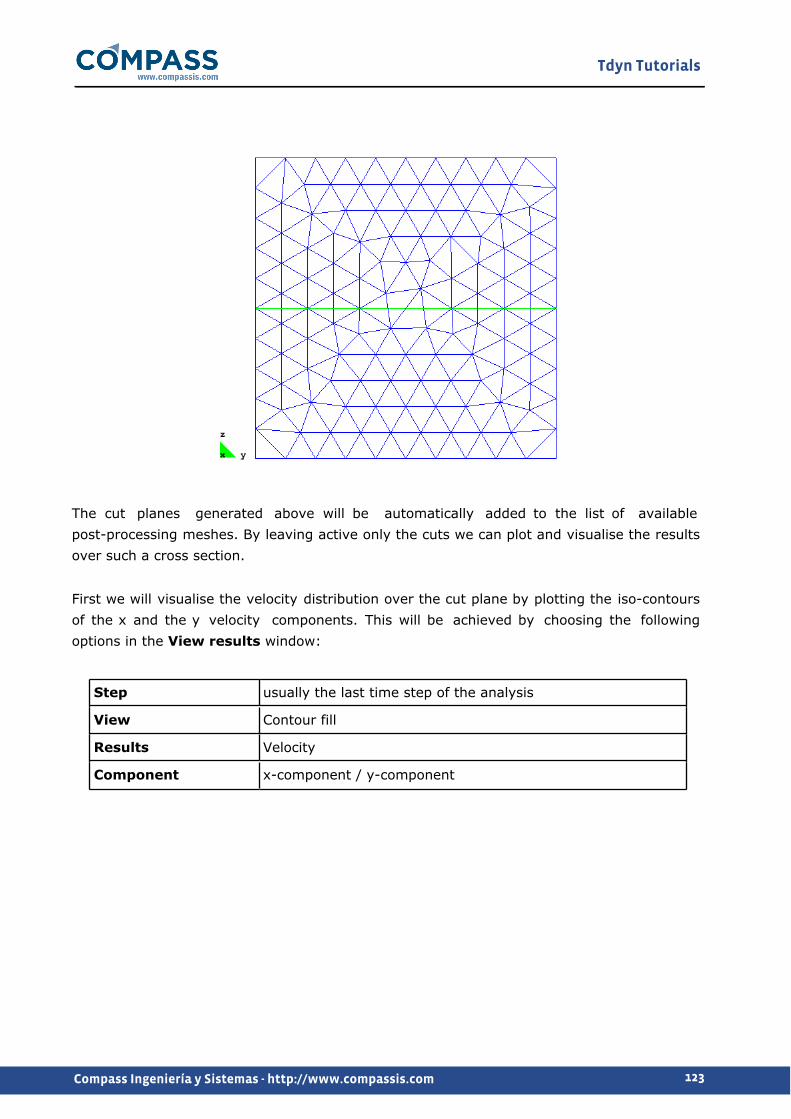
Tdyn Tutorials


The cut planes generated above will be automatically added to the list of available post-processing meshes. By leaving active only the cuts we can plot and visualise the results over such a cross section.

First we will visualise the velocity distribution over the cut plane by plotting the iso-contours of the x and the y velocity components. This will be achieved by choosing the following options in the View results window:

Step usually the last time step of the analysis

View Contour fill

Results Velocity

Component x-component / y-component

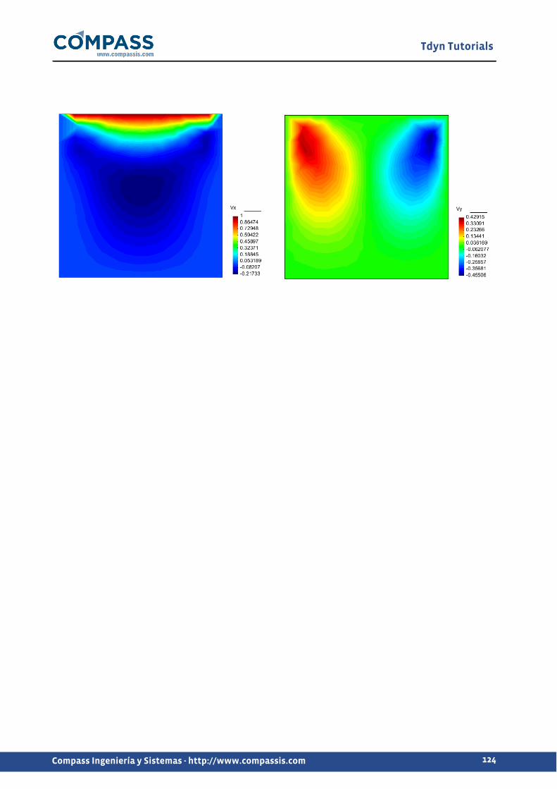
Tdyn Tutorials


Tdyn Tutorials


Laminar flow in pipe

Introduction

This example shows the analysis of a fluid flowing through a circular pipe of constant cross-section. The pipe diameter is D=0.2 m and length L=8 m. The inlet velocity of the flow Vin=1 m/s. Consider the velocity to be constant over the inlet cross-section. The fluid

exhausts into the ambient atmosphere which is at a relative pressure of 0.0 Pa.

Taking a density ρ=1 kg/m3 and viscosity µ= 2·10-3 kg/m·s, the Reynolds number Re based on the pipe diameter is:

Re=(ρ·Vin·D)/µ=100

Since the problem has symmetry about the pipe axis, the axisymmetric module of Tdyn will be used for the analysis.

Start data


2D Axisymmetric

Tdyn Tutorials


Flow in fluids


Pre-processing

The geometry used in this example is shown in the figure of the introduction section of the present tutorial. It represents one half cross-section of the pipe, since by symmetry the asisymmetric module has been used.

Boundary conditions

Once the geometry of the control domain has been defined, we can proceed to set up the boundary conditions of the problem (access the conditions menu as shown in example 1). The only conditions to be specified in this example are the inlet velocity and the outlet pressure on the pipe. Inlet velocity is fixed to 1.0 m/s in the positive Y direction on the bottom edge of the pipe,

Conditions & Initial Data Fluid Flow Inlet

while pressure is fixed to 0.0 on the top edge (see figure below).

Conditions & Initial Data Fluid Flow Outlet

Inlet/Outlet condition

Tdyn Tutorials


Materials

Physical properties of the materials used in the problem are defined in


Some predefined materials already exist, while new material properties can be also defined if needed. In this case, only Fluid Flow properties need to be defined. For the present example, fluid flow properties present in the default Generic Fluid can be used so that only viscosity must be changed to the value 2e-3 Kg/m·s.



This set of properties must be assigned to the only existing surface of the model (that defining the control volume of the present 2D axisymmetric case).


Boundaries

Fluid Wall/Bodies

The next step in the setup of the analysis is the definition of the wall properties of the pipe. In the present case the wall boundary type must be set to V FixWall, and the corresponding Wall/Body condition must be finally assigned to the line in the right side of the model, which defines the external surface of the pipe.


Problem data

Generic data of the problem must be entered to complete the analysis definition. Those fields whose default values should be modified are the following ones:


Tdyn Tutorials


Number of steps 500

Time increment 0.01 s.

Max. Iterations 1

Initial steps 0


Mesh generation

The mesh to be used in this example will be structured and composed of 400 x 40 linear quad elements. Structured type will be specified for all lines of the model. 400 equal-spaced divisions must be assigned to vertical lines, while 40 divisions are assigned to the top and bottom lines of the model in conjunction with the concentate elements option.

Mesh Structured Lines Concentrate Elements

In this case, a value 0.2 is given to the End Weight of the concentrate elements option as to ensure a good resolution of the boundary layer close to the wall of the pipe.

Tdyn Tutorials


Detail of the mesh

Calculate


Post-processing

When the calculations are finished, the message Process '...', started on ... has

Tdyn Tutorials


finished. is displayed. Then we can proceed to visualise the results by pressing the Postprocess icon (the problem must be still loaded or if this not the case, we should have to open the problem files again).

For details on the results visualisation not explained here, please refer to the Postprocessing chapter of the previous examples and to the Postprocess reference manual.

Some results of the analysis are shown below.

The velocity profile resulting of the analysis can be compared with the well-known analytical solution of the laminar flow in a circular pipe obtained by Hagen-Poiseuille (R is the radius of the pipe):

V=Vmax·(1-(x/R)2)

Axial velocity profile in a radius (outlet section)

The Hagen-Poiseuille solution also gives a formulation for the friction factor in pipes:

Cf = 2·τw/(ρ·Vm2 )=16/Re

For Re = 100, Cf = 0.16. This figure is identical to that obtained with CompassFEM in the

outlet section of the pipe.

Tdyn Tutorials


Turbulent flow in pipe

Introduction

This example shows the analysis of a fluid flowing through a circular pipe of constant cross-section. The pipe diameter is D=0.2 m and length L=8 m. The inlet velocity of the flow Vin=1 m/s. Consider the velocity to be constant over the inlet cross-section. The fluid

exhausts into the ambient atmosphere which is at a relative pressure of 0.0 Pa.

Taking a density ρ=1 kg/m3 and viscosity µ= 10-5 kg/m·s, the Reynolds number Re based on the pipe diameter is:


Since the problem has symmetry about the pipe axis, the axisymmetric module of Tdyn will be used for the analysis.

Start data


2D Axisymmetric

Tdyn Tutorials


Flow in fluids


Pre-processing

The geometry used in this example is shown in the figure of the introduction section of the present tutorial, and is identical to that concerning the previous example Laminar flow in pipe -pag. 125-. As in the previous example, it represents one half cross-section of the pipe, since by symmetry the asisymmetric module can be used.

Boundary conditions

Once the geometry of the control domain has been defined, we can proceed to set up the boundary conditions of the problem (access the conditions menu as shown in example 1). The inlet velocity and outlet pressure conditions to be applied are exactly the same as in the previous example (see Boundary conditions -pag. 126-). The actual value of the Reynolds number is imposed by just changing the viscosity of the fluid (see Materials -pag. 132-).

Materials

Some predefined materials already exist, while new material properties can be also defined if needed. In this case, only Fluid Flow properties need to be defined. For the present example, fluid flow properties present in the default Generic Fluid can be used so that only viscosity must be changed to the value 1e-5 Kg/m·s.

Materials Physical Properties Generic Fluid Generic Fluid1 Fluid Flow Viscosity


This properties must be assigned to the only existing surface of the model (that defining the control volume of the present 2D axisymmetric case).


Boundaries

Fluid Wall/Bodies

Tdyn Tutorials


The next step of the process is the definition of the wall properties of the pipe.


As in the previous example, Boundary type must be set to V FixWall, and the corresponding Wall/Body can be finally assigned to the line on the right side of the model, which defines the external surface of the pipe.

Problem data

Generic data of the problem must be entered to complete the analysis definition. Those fields whose default values should be modified are the following ones:


Number of steps 500

Time increment 0.01 s.

Max. Iterations 1

Initial steps 0


Modules data

Because of the conditions of the problem treated in this tutorial, turbulence effects will appear. In this case, the K_E_High_Reynolds model will be selected.

Modules Data Fluid Flow Turbulence Turbulence Model K_E_High_Reynolds

Fix Turbulence on Bodies option may retain its default value Auto.

Modules Data Fluid Flow Turbulence More... Fix Turbulence on Bodies Auto

Mesh generation

The mesh to be used in this example is the same as in the previous tutorial. In fact, that mesh was already defined as to fulfill the boundary layer requirements of the present case. In

Tdyn Tutorials


this sense, the mesh must be adequate to accurately solve the problem within the boundary layer region. To this aim, the fundamental requirement is that at least two points of the mesh must be located within the viscous sublayer.

The thickness of the viscous sublayer can be estimated as (y+ ≤ 5):

δν=5·μ/√(ρ·τw)

The wall stress τw will be estimated using the Colebrook-White law, that estimates the friction

factor in circular ducts:

1/√(4·Cf)=-2·log10(2.51/(Re·√(4·Cf)))

The estimated value from the above formula for Cf is 0.0065, and therefore:

τw = 1/2·ρ·Vm2 ·Cf = 0.0033 Kg/(m·s2)

Finally,

δν=5·μ/√(ρ·τw)=8.7·10-4m

And therefore, the second grid point of the mesh must be located within that distance. In our case, the second grid point is at 3.1·10-4 m (see the figure below).

Detail of the mesh within the boundary layer region

Tdyn Tutorials


Initial data

Initial values for turbulence parameters must be fixed before calculation. In particular, the EddyKEner Field and the EddyLength Field must be fixed as shown in the following figure:

Conditions & Initial Data Initial and Conditional Data Initial and Field Data EddyKEner Field

Conditions & Initial Data Initial and Conditional Data Initial and Field Data EddyLength Field

Calculate


Post-processing

First, the lenght of the transition region of the pipe can be evaluated. To this aim, the border graph capabilities of the postprocess GiD module can be used. See manual for further details on postprocessor options.

Tdyn Tutorials


Axial velocity evolution at the centerline of the pipe

As can be seen in the figure, the fluid does no longer accelerate once the fluid flow is fully developed. Such a transition occurs at a position along the pipe located about 6 meters from the inlet.

Next figure shows the axial velocity distribution in the outlet section of the pipe.

Finally, the velocity, pressure and eddy viscosity fields resulting from the simulations are shown in the following figure:

Tdyn Tutorials


Results summary

Several cases have been simulated, for which the friction coefficient results are summarized in the following table. For the sake of comparison, reference data has been estimated from the Colebrook-White and Hagen-Poiseuille laws:

Re Cf (CompassFEMFD&M) Cf (Reference)

100 0.16 0.16

5000 0.0120 0.0093

10000 0.0088 0.0077

Tdyn Tutorials


20000 0.0066 0.0065

40000 0.0045 0.0055

For the case Re = 40000, TIL = 10% has been used since values less than 8% do not provide a steady state solution.

Appendix

Additional information

The experimental friction factor (Cf) for laminar flow (Vm is the mean flux) is given by the

Hagen-Poiseuille solution:

Cf = 2·τw/(ρ·Vm2 )=16/Re

where τw is the shear stress in the wall, which for laminar flow in circular pipes is also given

by the well-kwon solution (Hagen-Poiseuille):

τw=4·μ·Vm/R

It is also used the Darcy's friction factor λ = 4·Cf. See the following link:

http://en.wikipedia.org/wiki/Swamee-Jain_equation

For non-roughness pipes, it can be estimated from:

1/√λ=-2·log10(2.51/(Re·√λ))

Blasius' curve: Cf = 0.0791·ReD-1/4

Prandtl's curve: 1/√λ=-2·log10((Re·√λ))-0.8

The hydraulic diameter for a pipe is defined as:

Dh=4·A/P

where A is the area of the cross section and P its perimeter.

Tdyn Tutorials


Laminar and turbulent flows in a 3D pipe

Introduction

This tutorial is a 3D extension of the previous 2D examples which concerned the analysis of laminar and turbulent flows in a pipe. Both, laminar and turbulent cases are reproduced here for a true 3D geoemtry. Hence, material properties and boundary conditions are exactly the same as in the two previous tutorials. The objective of the present example is to present the 3D capabilities of Tdyn-CompassFEMand in particular the 3D boundary layer meshing tool.

For the laminar case, taking a density ρ=1 kg/m3 and viscosity µ= 2·10-3 kg/m·s, the Reynolds number for an inlet velocity V=1 m/s based on the pipe diameter D = 0.2 m is:


For the turbulent case, taking a density ρ=1 kg/m3 and viscosity µ= 10-5 kg/m·s, the Reynolds number Re based on the pipe diameter, for the same inlet velocity is:


Start data


3D Flow in fluids


Pre-processing

The geometry used in this example consists on a circular pipe with constant cross section. The diameter of the pipe is D=0.2m and its length is L=8m. In the present case, a 3D model representing a 90º section of the pipe is simulated. Pertienent symmetry conditions are imposed on the lateral surfaces of the model in order to reproduce the full symmetry of revolution of the problem (see section Boundary conditions -pag. 140-).

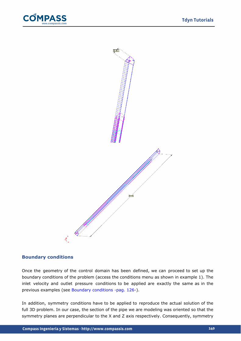
Tdyn Tutorials


Boundary conditions

Once the geometry of the control domain has been defined, we can proceed to set up the boundary conditions of the problem (access the conditions menu as shown in example 1). The inlet velocity and outlet pressure conditions to be applied are exactly the same as in the previous examples (see Boundary conditions -pag. 126-).

In addition, symmetry conditions have to be applied to reproduce the actual solution of the full 3D problem. In our case, the section of the pipe we are modeling was oriented so that the symmetry planes are perpendicular to the X and Z axis respectively. Consequently, symmetry

Tdyn Tutorials


conditions can be enforced by imposing a null velocity component condition along the direction perpendicular to the symmetry planes. This is done by using the following velocity field conditions that must be applied to the X=0.0 and Z=0.0 symmetry planes respectively:

Conditions & Initial Data Fluid Flow Velocity Field Fix Initial X

Conditions & Initial Data Fluid Flow Velocity Field Fix Initial Z

Materials

Physical properties of the materials used in the problem are defined in the following section of the CompassFEM Data tree.


Some predefined materials already exist, while new material properties can be also defined if needed. In this case, only Fluid Flow properties are relevant for the analysis, and those properties present in the default Generic Fluid can be reused so that only viscosity must be changed to fullfil the actual Reynolds number we are interested in. For the laminar case, viscosity is fixed to μ=2·10-3 kg/ms, while for the turbulent case it is set to μ=1·10-5 kg/ms. For each material parameter, the corresponding units have to be verified, and changed if necessary (in our example, all the values are given in default units). The fluid flow set of properties must be finally assigned to the volume that defines the bulk domain of the pipe.


Boundaries

Fluid Wall/Bodies

The next step of the process is the definition of the wall properties of the pipe.


As in the previous example, the Wall/Body boundary type must be so that it strictly enforces the no slip condition at the wall (null velocity). Hence, the pertinent condition to be applied is:

Conditions & Initial Data Fluid Flow Wall/Bodies Boundary Type V FixWall

Tdyn Tutorials


Such a condition must be finally assigned to the external surfaces of the pipe.

Problem data

Some generic data of the problem must be updated in accordance to the particular operating conditions of the model. Hence, the options in the table below must be modified depending on the actual flow regim of the problem under analysis (laminar or turnulent):


Laminar flow

Number of steps 500


Max. iterations 1

Initial steps 0


Turbulent flow



Max. iterations 1

Initial steps 0


Remark:

Time increment for the turbulent case has been reduced since the longitudinal element size for this case (i.e. along the main flow direction) limits the maximum value allowed to obtain good convergence of the solution.

Modules data

Default values of Modules data can be used for the laminar flow case. On the other hand, for the turbulent flow simulation a pertinent turbulence model must be especified. In this case, we will choose the K_E_High_Reynolds model.

Tdyn Tutorials


Modules Data Fluid flow Turbulence Turbulence Model K_E_High_Reynolds

Fix Turbulence on Bodies option can retain its delault value Auto. Advanced turbulent options must retain also their default values as shown in the figure below.

Modules data Fluid flow Turbulence More...

See Mesh generation -pag. 143- for details on the estimation of turbulence parameters initial values.

Mesh generation

The mesh to be used must be adequate to accurately solve the problem within the boundary layer region. To this aim, the fundamental requirement is that at least two points of the mesh must be located within the viscous sublayer. All necessary calculations to estimate the boundary layer parameters have been described in the previous examples. For the present case, the following data must be used for the calculation of the boundary layer parameters.

Laminar flow

Diameter 0.2 m

Inlet velocity 1 m/s

Viscosity 2e-3 kg/m·s

Tdyn Tutorials


Density 1 kg/m3

Turbulent flow

Diameter 0.2 m

Inlet velocity 1 m/s

Viscosity 1e-5 kg/m·s

Density 1 kg/m3

On the second page of the form we should provide the friction coefficient that can be obtained, for a given Reynolds number, by solving graphically or numerically the Colebrook-White law (see Mesh generation -pag. 133-).

Once all this data has been entered, the form provides as an ouput the following parameters:

τW= friction stress at the wall

dv = boundary layer thickness

h1 = recomended thickness of the first element in the layer adjacent to the wall of the pipe

h = recomended longitudinal size of the boundary layer elements

TIL, Kt and Lt = turbulence parameters

Kt and Lt values must be entered in the EddyKEner and EddyLength fields respectively.

Conditions & Initial Data Initial and conditional data Initial and Field Data EddyKEner Field

Conditions & Initial Data Initial and conditional data Initial and Field Data EddyLength Field

Boundary layer parameters represent a more severe restriction over the mesh generation in the turbulent case, since the thickness of the first layer is much smaller. The following figures show the mesh properties assignment used to construct the meshes that fullfil the previously evaluated boundary layer characteristics.

First, a semi-structured mesh can be constructed so that tetrahedral elements can be used. In this case an automatic boundary layer mesher is available. The options used to construct the mesh for the turbulent case are shown in the following figures.

Tdyn Tutorials


As shown in the tables above, for the present turbulent case (Re=20000) the first element next to the boundary wall must have a thickness h1=2.9x10-4 m. Tdyn has been extensively

tested to estimate the maximum aspect ratio the elements can support without loosing convergence. For the present case, a sensible value for the maximum allowed aspect ratio is about 125. Hence, the maximum element size along the pipe axis direction is h ≈ 125·h1 =

0.036 mwhich for a pipe length of 8 m. results in about 220 element divisions along the pipe.

The boundary layer is constructed using the following parameters:

Tdyn Tutorials


In order to ensure the mesh at the wall boundary surface is structured and smooth, it is necessary to deactivate the "symmetrical structured options" in the meshing preferences.

Utilities Preferences Meshing Structured mesh

If these options are not deactivated, the generated mesh becomes symmetric but the circular perimeter of the pipe results in a saw shape with sharpe edges that is unacceptable for this kind of problem.

The resulting mesh consists of 37128 nodes and 211413 tetrahedral elements.

Alternatively, a completely unstructured mesh can be used. Nevertheless, in this case the number of divisions along the pipe axis direction must be significantly increased (about 500 divisions) to avoid the existence of too much distorted elements. This implies also that the time increment must be decreased in order to achieve convergence. In this case, the final mesh consists of 65333 nodes and 366844 elements.

Tdyn Tutorials


Initial data

Initial values for turbulence parameters must be fixed before calculation. In particular, the EddyKEner Field and the EddyLength Field must be fixed as shown in the following figure:

Conditions & Initial Data Initial and Conditional Data Initial and Field Data EddyKEner Field

Conditions & Initial Data Initial and Conditional Data Initial and Field Data EddyLength Field

Calculate

The calculation process will be started from within GiD through the Calculate menu, as it has

Tdyn Tutorials


been described in previous examples.

Post-processing

First, the lenght of the transition region of the pipe can be evaluated. To this aim, the graph capabilities of the postprocess module can be used.

As can be seen in the figure, the fluid does no longer accelerate once the fluid flow is fully developed. Such a transition occurs at a position along the pipe located about 6 meters from the inlet.

Next figure shows the axial velocity distribution in the outlet section of the pipe. To this aim, generate a line cut following a radius of the outlet section of the pipe.

Tdyn Tutorials


Finally, the velocity, pressure and eddy viscosity fields resulting from the simulations are shown in the following figure:

Tdyn Tutorials


Tdyn Tutorials


Ekman's Spiral

Introduction

The application of TCL script programming in Tdyn-CompassFEM is discussed in this tutorial. The objective is to give the reader/user of Tdyn-CompassFEM an idea on how to extend the capabilities of CompassFEM through the introduction of the aforementioned scripting tool. As a case study the solution of the Ekman's spiral has been choosen. Interest in this subject goes back since the publication of Ekman's work and since then, various references and articles have discussed the solution to the Ekman's spiral. Among these publications are "Introductory Dynamical Oceanography" by Pönd and Picard (1983) and "Large-eddy simulation of the wind-induced turbulent Ekman layer" by Zikanov, O. (2003).

Problem formulation

When wind blows over the surface of the water, energy in the form of momentum is transferred from the air to the water. A turbulent flow near the ocean surface is generated by this steady wind stress in the presence of Earth's rotation. To study the effect of the wind stress, Ekman used the following assumptions to derive a solution now known as the "Ekman's spiral":

Domain without boundaries Infinite depth Constant vertical eddy viscosity Steady wind blowing with constant velocity Constant density Constant Coriolis parameter

Assuming a hydrostatic pressure field, the steady momentum equations for this problem are as follows:

f·vE + νv (∂2uE)/(∂z2) = 0

-f·uE + νv (∂2vE)/(∂z2) = 0

where f = 2·Ω·sinΦ is the Coriolis parameter, with Ω and Φ the Earth's rotation rate and latitude respectively, vE and uE the cartesian components of the mean horizontal velocity,

vv is the vertical kinematic viscosity and z is the vertical coordinate directed downward. In the

case of a setady wind in the horizontal direction, the solution of the above equations for finite depth (the so-called Ekman velocity profile) is:

Tdyn Tutorials


uE = Vo cos(π/4+π·z/DE)exp(π·z/DE)

vE = Vo sin(π/4+π·z/DE)exp(π·z/DE)

where DE = π(2vv/f)1/2 is the Ekman depth of exponential decay, and Vo is the steady state

surface velocity. According to the solution, the mean horizontal current spirals clockwise and decay exponentially with depth. In the surface, the velocity is directed 45º to the right (northern hemisphere) or the left (southern hemisphere) of the wind direction.

It is trivial to see that for the given velocity profile, the momentum equations are satisfied, since:

(∂2u)/∂z2 = -2·v·(π/D)2

(∂2v)/∂z2 = 2·u·(π/D)2

It is also noted, that for this solution the advection term of the momentum equations vanishes, and then the above presented equations are valid in the steady state. Furthermore, the continuity equation is also trivially satisfied, since:

∂u/∂x = ∂v/∂y = w = 0

Finally, the natural boundary conditions for the above equations are (for bottom and water surface):

τx = μ·∂u/∂z = (μ·π·(u-v))/D

Tdyn Tutorials


τy = μ·∂v/∂z = (μ·π·(u+v))/D

Evaluating those relations for z=0, results:

τx = 0

τy = μ·∂v/∂z = √2·μ·V·π/D

And therefore, the surface velocity is given by:

V = (√(2)·π·τv)/(D·ρ·f)

Being τv, the surface shear stress generated by the wind.

The analytic solution of the Ekman's spiral for a finite depth H is given by:

uE = A·sinh(a(H-z))·cos(a(H-z)) - B·cosh(a(H-z))·sin(a(H-z))

vE = A·cosh(a(H-z))·sin(a(H-z)) + B·sinh(a(H-z))·cos(a(H-z))

The parameters A and B are defined as follows:

A = (τv·D/μ·π)·(cosh(aH)·cos(aH)+sinh(aH)·sin(aH))/(cosh(2aH)+cos(2aH))

B = (τv·D/μ·π)·(cosh(aH)·cos(aH)-sinh(aH)·sin(aH))/(cosh(2aH)+cos(2aH))

Being μ, the vertical kinematic viscosity. It can be easily seen that for the above presented solution, the following relations are satisfied:

(∂2u)/∂z2 = -2·v·a2

(∂2v)/∂z2 = 2·u·a2

And therefore, momentum equations are satisfied for f = 2·νv·a2, or a = ((Ω·sinΦ)/νv)1/2,and

then D = π/a.

As in the previous infinite depth case, the continuity equation is trivially satisfied, since:

∂u/∂x = ∂v/∂y = w = 0

Start data

Tdyn Tutorials


In order to solve the Ekman's spiral, the following type of problems must be loaded in the Start Data window of the CompassFEM suite.

3D Flow in fluids


Pre-processing

Three case studies are to be analysed in this tutorial in order to compare results of the Ekman solution for infinite and finite depth. In the different cases, the vertical kinematic viscosity is taken equal to 0.014 m2/s and a latitude Φ = 45º is assumed. Hence the Ekman's depth of exponential decay results to be D = π(2vv/f)1/2 = 51.76 m.

The wind stress applied to the surface is τv = 0.001638 Pa, corresponding to a wind speed of

30m/s.

Three different geometries were used for the different case studies. A of the and boundary conditions to be applied in every case is given next. In the second case, a computational domain depth Lz = D/2 = 25.88 m will be used. In that case, the finite depth solution of the

Ekman's spiral is obtained. Finally, a third case with Lz = D/3 = 17.25 m will be analysed.

However, in this case, the stress given by the infinite depth solution will be imposed at the bottom surface, and therefore, the infinite depth solution will be obtained again.

Case 1:

In the first case, a computational domain of dimensions Lx x Ly x Lz = 100 m x 100 m x 100

m will be used. Since the depth is almost twice the depth of Ekmar exponential decay, the infinite depth solution is expected to be found.

The boundary conditions to be applied in this case are:

top surface: normal velocity is set to 0.0 and wind stress is imposed using a TCL script.

bottom surface: null velocity is imposed.volume: pressure is fixed to 0.0.

Remarks: Imposing null pressure in the volume is equivalent to assume that a hydrostatic pressure is maintained during the simulation. In fact, this is only valid for the steady state of the problem. However, this simplification helps to improve the stability of the solution process and to find faster the steady solution.

Tdyn Tutorials


The momentum equations of the problem assume that the horizontal derivaties of the velocity are null, or equivalently that the corresponding viscous stresses terms can be neglected. The strategy selected in this case to fulfil this requirement is to solve the following modified equations:

f·v+ νv·(∂2u)/∂z2 = -νa·(∂2u)/∂x2- νa·(∂2u)/∂y2

-f·u + νv·(∂2v)/∂z2 = -νa·(∂2v)/∂x2- νa·(∂2v)/∂y2

The natural boundary conditions of the problem guarantee that the terms at the right hand side vanish at the steady state. Anyhow, it is advisable to select νa << νv. This is done by

means of a TCL script.

Case 2:

In the second case, a computational domain depth Lz = D/2 = 25.88 m will be used (Lx x Ly x

Lz = 100 m x 100 m x 25.88 m). In that case, the finite depth solution of the Ekman's spiral

is obtained.


top surface: normal velocity is set to 0.0 and wind stress is imposed using a TCL script. bottom surface: null velocity is imposed.

Remark: In this case, pressure field is solved during the computation. However, it will be verified that the obtained steady pressure gradient field is actually negligible, as expected.

The strategy to solve the momentum equations is identical to that used in the first case.

Case 3:

Finally, a third case with Lz = D/3 = 17.25 m will be analysed (Lx x Ly x Lz = 100 m x 100 m

x 17.25 m). However, in this case, the stress given by the infinite depth solution will be imposed at the bottom surface, and therefore, the infinite depth solution will be obtained again.


top surface: normal velocity is set to 0.0 and wind stress is imposed using a TCL script. bottom surface: normal velocity is set to 0.0 and solution stress is imposed using a TCL script. volume: pressure is fixed to 0.0.

The strategy to solve the momentum equations is identical to that used in the previous cases.

Boundary conditions

Tdyn Tutorials


Once the geometry of the control domain has been defined, we can proceed to set up the boundary conditions of the problem.

Case 1:

A new fluid boundary must be created and named "wind".

Conditions & Initial Data Fluid Flow Wall/Bodies group: wind

Such a condition will represent the wind stress acting on the top surface of the domain. Hence the new fluid boundary must be assigned to the aformentioned top surface of the model geometry. For such a wall, the boundary type must be Invis Wall as shown in the fiugre, so that it imposes the slipping condition on the boundary (i.e. wall normal velocity component will be zero).

In addition, the value of the wind stress imposed on the surface boundary is 1.82e-01 N/m2 and will be fixed through the TCL script on all nodes pertaining to the assigned "wind" group. This boundary condition is the only one imposed for the case study number 1.

Case 2:

Aside from the wind stress acting on the top surface boundary, an additional boundary condition is introduced in Case 2. In this sense, an inviscid wall boundary condition is also imposed to the bottom surface of the fluid domain. The value of the wind stress imposed on the surface boundary is 1.82e-01 N/m2 as in the previous case.

Case 3:

Tdyn Tutorials


The boundary conditions in Case 3 are similar to those in Case 2. The same wind stress is imposed on the top surface of the domain and an inviscid wall boundary condition is imposed at the bottom.

Materials

The same material is used in the three case studies. The physical properties of the present fluid are specified using the already defined Generic_Fluid1 material.

Actually, the density and the horizontal viscosity of the fluid must be changed and their values set to 1000 kg/m3 and 1.0e+06 kg/m·s respectively. Nevertheless, this values are actually set through the TCL script, so that at the user interface level just the corresponding functions implemented in the TCL script must be invoked as shown in the following figure (i.e. tcl(set den) or tcl(set vis)).

Materials Physical Properties Generic Fluid Generic_Fluid1 Fluid Flow Density


The calculation of the acceleration field due to the Coriolis effect must be also performed through a tcl script function. This is indicated at the user interface level by invoking the tcl(calcOx) and tcl(calcOy) functions from the corresponding acceleration fields.

Tdyn Tutorials


Materials Physical Properties Generic Fluid Generic_Fluid1 Acceleration Field X

Materials Physical Properties Generic Fluid Generic_Fluid1 Acceleration Field Y

Finally, since the fluid is anisotropic, the viscosity is also corrected in the TCL script by overwritting the contribution of the vertical viscosity to the system matrix. This is implemented by introducing the following line in the TCL script:

:: mather::matrix_vector_mult_add_fvsys $visc fdnz_dnz 1

(see Appendix (TCL script) section for more details on the funcionalities added by means of the TCL script).

Problem data

Some generic data must be entered to correctly define the analysis. Those fields whose default values should be modified for the present analysis are the following ones:



Time increment if(step<500)then(100.0)else(10.0)endif

Maximum iterations 3

Initial Steps 0


Results are taken every 25 steps and we are mainly interested on the pressure and velocity fields.

Fluid Dynamics & Multi-Physics Data Results Output Step 25

Fluid Dynamics & Multi-Physics Data Results Fluid Flow Write Velocity

Fluid Dynamics & Multi-Physics Data Results Fluid Flow Write Pressure

Tdyn Tutorials


Remember to activate the Use Tcl External Script option and to indicate the actual path for the location of the TCL script file.

Fluid Dynamics & Multi-Physics Data Other tcl data Use Tcl External Script

Modules data

For the present case, it is necessary to modify the default value of the StabTauP MinRatio parameter in the Modules Data->Fluid Flow->General window. Such a parameter should be fixed to 0.01 in order to achieve accurate results.

Modules data Fluid flow Algorithm

Mesh generation

In this case, linear hexahedral elements are employed in the mesh. To this aim structured mesh conditions are assigned to all surfaces and to the volume of the domain. Hexahedra element type is assigned to the volume as well. 4 divisions are assigned to the edges of the cube that are parallel to the top and bottom surfaces, while 30 divisions are assigned to the vertical edges. An element concentration must be also assigned to these perpendicular edges so that the elements close to the top surface exhibit a height/width ratio about 0.1 (see mesh properties assignement in the figures below).

Tdyn Tutorials


Calculate



Post-processing

Tdyn Tutorials


Upon completion of the calculation process, we can proceed to visualize the results by pressing the postprocess icon in the toolbar menu or by accessing the main menu Files->Postprocess. In all three case studies the results concerning the velocity vector fields can be drawn through the option View results->Display Vectors->Velocity->|V|. The corresponding results are shown in the figures below:

Case 1: Velocity vector field (general view)

Tdyn Tutorials


Case 1: Velocity vector field (top view)

Case 2: velocity vector field (general view)


Tdyn Tutorials


Case 3: velocity vector field (general view)


Appendix (TCL script)

Source Code of the TCL Script

# Fluid density with the value to be defined by the user set den 1000.0

Tdyn Tutorials


# Fluid 'horizontal' viscosity with the value to be defined by the user set vis 0.14

# Fluid 'vertical' viscosity with the value to be defined by the user set vsz 14.0

proc calcOx { } { # Read the index of the current node set inode [TdynTcl_Index 0] set Vey [TdynTcl_VecVal vy $inode] return [expr {2*7.292e-05*sin(45*(3.1415926/180.0))*$Vey}]}

proc calcOy { } { set inode [TdynTcl_Index 0] set Vex [TdynTcl_VecVal vx $inode] return [expr {-2*7.292e-05*sin(45*(3.1415926/180.0))*$Vex}]}

# Computation of the surface wind stress

proc TdynTcl_InitiateProblem { } { global sstress bstress visc staux stauy btaux btauy vis vsz

TdynTcl_Message "Executing script imposing stress on water surface and bottom" notice # Value of wind stress # Tau = Coef_arrastre * Rho_aire/Rho_agua * (Velocidad_viento)^2 # Tau = 0.0014 * 1.3/1000 * (30 m/s)^2 set staux 0.0 set stauy 0.001638 set btaux 0.0 set btauy 0.0

# Read the indexes of the nodes of the fluid body wind set nodes [TdynTcl_GetFluidBodyNodes wind]

Tdyn Tutorials


# Create a vector (surface stress) set nnode [TdynTcl_NNode 1] set tract [::mather::mkvector $nnode 0.0] foreach inode $nodes { set jnode [TdynTcl_GlobalToFluid $inode] ::mather::setelem $tract $jnode 1.0 } # Compute the FEM integral set sstress [::mather::vmexpr temp=fwind*$tract] # Delete the vector created previously ::mather::delete $tract

# Read the indexes of the nodes of the fluid body bottom set nodes [TdynTcl_GetFluidBodyNodes bottom] # Create a vector (surface stress) set nnode [TdynTcl_NNode 1] set tract [::mather::mkvector $nnode 0.0] foreach inode $nodes { set jnode [TdynTcl_GlobalToFluid $inode] ::mather::setelem $tract $jnode 1.0 } # Compute the FEM integral set bstress [::mather::vmexpr temp=fbottom*$tract] # Delete the vector created previously ::mather::delete $tract

# Compute the nodal dynamic vector viscosity Mu = Upsilon * Rho_agua # vval = Kv - Kh = 14.0 - 1.0e+6 = -999986.0 kg/(m.s) set vval [expr $vsz-$vis] set nnode [TdynTcl_NNode 1] set visc [::mather::mkvector $nnode $vval]}

# Apply the x component of the wind stress

Tdyn Tutorials


proc TdynTcl_AssembleFluidMomentumX { } { global sstress bstress visc staux stauy btaux btauy

# Assemble the stress terms set nnode [TdynTcl_NNode 1] for {set inode 1} {$inode <= $nnode} {incr inode} { set jnode [TdynTcl_FluidToGlobal $inode] set ri [TdynTcl_GetRhs $jnode] set tsi [expr [::mather::getelem $sstress $inode]*$staux] set tbi [expr [::mather::getelem $bstress $inode]*$btaux] TdynTcl_SetRhs $jnode [expr $ri+$tsi-$tbi] } # Assemble the viscosity terms ::mather::matrix_vector_mult_add fvsys $visc fdnz_dnz 1 }

# Apply the y component of the wind stress

proc TdynTcl_AssembleFluidMomentumY { } { global sstress bstress visc staux stauy btaux btauy

# Assemble the stress terms set nnode [TdynTcl_NNode 1] for {set inode 1} {$inode <= $nnode} {incr inode} { set jnode [TdynTcl_FluidToGlobal $inode] set ri [TdynTcl_GetRhs $jnode] set tsi [expr [::mather::getelem $sstress $inode]*$stauy] set tbi [expr [::mather::getelem $bstress $inode]*$btauy] TdynTcl_SetRhs $jnode [expr $ri+$tsi-$tbi] } # Assemble the viscosity terms ::mather::matrix_vector_mult_add fvsys $visc fdnz_dnz 1 }

Tdyn Tutorials


# Compute the constant turbulent diffusivity coefficient

proc TdynTcl_AssembleFluidMomentumZ { } { global temp visc

# Assemble the viscosity terms ::mather::matrix_vector_mult_add fvsys $visc fdnz_dnz 1 }

Tdyn Tutorials


Taylor-Couette flow

Introduction

This tutorial aims to demonstrate the application of user-defined functions and TCL script programming within the framework of the Tdyn-CompassFEM suite. The main goal of this tutorial is to give the reader/user of CompassFEM an idea on how to extend the intrinsic capabilities of CompassFEMby using the abovementioned tools. For the sake of illustration, the Taylor-Couette flow experiment was selected as a case study. Such a problem formulation has been taken from the book "Physical Fluid Dynamics" by D.J.Tritton. This choice responds to the following reasons:

The problem is simple and easy to understand User-defined functions or TCL script programming are essential for solving the problem

Problem formulation

The Taylor-Couette experiment consists on a fluid filling the gap between two concentric cylinders, one of them rotating around their common axis. The resulting fluid flow is called the Taylor-Couette flow which is used to validate the effect of the Coriolis force.

In the present analysis the aim is to solve the velocity distribution of a Newtonian fluid, with a kinematic viscosity vH = vV = v = 0.1 m2/s and a density ρ = 1 kg/m·s, that is contained in

the gap between two concentric cylinders characterized by a radius relation ξ = a/b = 0.5 and an aspect ratio λ = L/(b-a) = 2. The Reynolds number for this problem is given by:

Re = (Ω1a(b-a))/v = 1.9635

and the Ekman number is

Ek = v/(Ω1(b-a)2) = 0.509

See the figure below for an schematic representation of the Taylor-Couette flow experiment.

Tdyn Tutorials


Two different case studies were considered for the sake of comparison. In the first one, the inner cylinder rotates in the anti-clockwise direction with an angular velocity Ω1 = 0.19635

s-1 while the outer cylinder remains at rest (Ω2 = 0). A solution of the momentum equation

can be obtained assuming the velocity has azimuthal (θ) diretion everywhere, and both velocity and pressure are independent of θ and z cylindrical polar coordinates. These assumptions are based on the cylindrical symmetry of the problem.

Under these conditions, the continuity equation ∂uθ/∂θ = 0 is automatically satisfied, and the

azimuthal and radial components of the Navier-Stokes equation result to be:

(∂2uθ)/∂r2 + 1/r ∂uθ/∂r - uθ/r2 = 0

ρuθ2/r = - dp/dr

The corresponding boundary conditions read as follows:

u(a) = Ω1a = 0.19635 in r = a

u(b) = Ω2a = 0.0 in r = b

The solution uθ when the flow remains entirely azimuthal is as follows:

uθ = Ar + B/r

where the coefficients A and B are given by:

Tdyn Tutorials


A = (Ω2b2 - Ω1a2)/(b2-a2) = -6.545·10-2

B = ((Ω1-Ω2)a2b2)/(b2-a2) = 0.392699

Finally, the pressure results to be:

pθ = A2(r2)/2 + 2ABln(r) - (B2)/(2r2)

For the second case study, the inner cylinder velocity is held to zero, and the exterior cylinder rotates clockwise with a velocity u(b) = -0.392699 m/s and a Coriolis parameter f = 2Ω1sinΦ

= 0.392699, being Ω1 = 0.19635 s-1 and Φ=90º.

For the sake of comparison between the two case studies, the rotation velocity of the axes, defined as Ωxr is substracted from the results obtained in the second case.

Start data

In order to simulate the Taylor-Couette flow experiment, the following type of problems must be loaded in the Start Data window of the CompassFEM suite.

3D Flow in fluids


Pre-processing

The same geometry is used for the two case studies and simply consists on two concentric cylinders of height L = 2m with an inner radius a = 1m and an exterior radius b = 2m (see figure below).

Tdyn Tutorials


Boundary conditions

Once the geometry of the control domain has been defined, we can proceed to set up the boundary conditions of the problem.

Case 1 (Inner cylinder rotating):

A boundary condition must be applied to the interior cylinder wall in order to impose the velocity over the fluid layer attached to the

surface of the rotating cylinder. The corresponding velocity field can be specified through user-defined functions that can be inserted in the VelX and VelY fields of an Inlet Velc boundary type:


On the other hand, a zero velocity condition must be imposed over the exterior cylinder, while a null normal velocity condition must be assigned to the top and bottom surfaces of the control domain. These two conditions can be applied by using a V FixWall and an Invis Wall boundary types respectively:


Tdyn Tutorials


Case 2 (Outer cylinder rotating):

In this case, the inner cylinder is hold at rest so that a null velocity boundary condition should be imposed on the corresponding surface. Use V FixWall boundary type to define the boundary condition to be applied to the inner cylinder surface:


In the case of the external cylinder surface, user-defined functions for the velocity fields, VelX and VelY, can be used to define the inlet condition applied to the external surface. These user-defined functions, that define the inlet condition for the external cylinder, have the same magnitude as those used in Case 1 but the sign is changed so that the external surface now rotates in the clockwise direction:


Tdyn Tutorials


Vel X Field: f(0.19635*y)

Vel Y Field: f(-0.19635*x)

Materials

Case 1:

The material used in the present analysis is defined as usual using the following data tree sequence:

Materials Fluid Fluid Flow

The material is assumed to be incompressible and density and viscosity take the values 1kg/m3 and 0.1 kg/m·s respectively. The corresponding material must be assigned to the volume of the control domain.

Case 2:

The same material as in Case 1 is going to be used here. Nevertheless, since this case study is used to validate the Coriolis term, the pertinent acceleration field must be defined using the following data tree sequence:

Materials Fluid Fluid Flow

To this aim, the following functions should be introduced in the corresponding acceleration fields (see figure below):

X - acceleration field component = f·v = 2*0.19635*sin(90*pi/180)*vy

Y - acceleration field component = -f·u = -2*0.19635*sin(90*pi/180)*vx

where f = 2ωTsinΦ is the Coriolis parameter.

Tdyn Tutorials


Fluid flow window: definition of the Coriolis acceleration terms

Problem data

Other generic problem data must be entered in the Fluid Dyn. & Multi-phy. Data section of the data tree. Those fields whose default values should be modified are the following ones:

Fluid Dyn. & Multi-phy. Data->Analysis

Number of steps 90

Time increment 0.1

Max. iterations 1

Initial steps 0


Results are taken every 25 steps and we are mainly interested on the pressure and velocity fields.

In order to compare the results obtained in both case studies, the rotation velocity Ωxr in Case 2 must be somehow sustracted from the total velocity field. To this aim, additional user-defined variables may be introduced in Fluid Dyn. & Multi-phy. Data->Results->User Def. Functions window, so that the new variables will be available for visualization in the postprocessing module. Specifically, two new variables must be defined, each one representing the pertinent velocity component after sustraction of the

Tdyn Tutorials


corresponding Coriolis term (see figure below).

Remark:

Each velocity component is defined as an individual variable in the user defined functions window. If we want the results to be available as a vector in the postprocessing module, we must take care of using the same name in the definition of the three variables, just with the cartesian component X, Y or Z added to the end of the name. Therefore, in this case we should rename the variables as FluidFunctionX/Y/Z respectively as shown in the figure above.

TCL extension

An alternative procedure to solve the Taylor-Couette flow problem is by using the TCL extension capabilities of the CompassFEMFD&M. This consists on using a TCL script provided by

the user that extends the intrinsic options of CompassFEM through the definition of new functionalities required for the solution of the particular problem at hand. In our case, the TCL script is going to be used to replace some of the user-defined functions and values introduced for the standard solution procedure described in the preceding sections (see Boundary conditions -pag. 171- and Materials -pag. 173-). The source code of the TCL scripts used for both case studies can be found in Appendix 1 -pag. 181- and Appendix 2 -pag. 182-.

In order to use the TCL script, some functions implemented within its source code need to be invoked at the user interface level. This is the case for instance when defining the material properties. In both, Case 1 and Case 2, the values specified in the density and viscosity fields of the materials definition should be replaced by the following calls to the TCL script functions:

Tdyn Tutorials


Materials Physical properties Generic fluid Fluid flow

Density: tcl(set den)

Viscosity: tcl(set vis)

This way, the values specified within the TCL code will be directly assigned to the corresponding material properties.

In Case 2, it is also necessary to indicate that the Coriolis acceleration terms are going to be calculated through the TCL script. Becuase of this, the following calls to TCL implemented functions must be introduced in:


X - acceleration field component = tcl(calcOx)

Y - acceleration field component = tcl(calcOy)

Similarly, some replacements are necessary for the specification of boundary conditions. Along these lines, the velocity field values that define the Inlet Velc boundary assigned to the interior cylinder wall in Case 1 and to the external cylinder surface in Case 2, can be alternatively specified by calling TCL functions as shown below. These function calls replace the user-defined values introduced in previous sections.

Vel X Field: tcl(calcVx)

Vel Y Field: tcl(calcVy)

The remaining boundary conditions were not described by user-defined functions/values. Therefore, no TCL script counterparts are implemented and the application of those boundary conditions remains the same as in the previous standard procedure.

Remember that when using the TCL extension, it is necessary to activate the Use Tcl External Script option in the data tree and to indicate there the actual path for the location of the required TCL script.

Fluid dynamics and multiphysics data Other Tcl data

Mesh generation

Tdyn Tutorials


In this case, the volume domain is discretized using linear hexahedral elements. 20 elements are used for discretization along the circumferential direction, while 8 and 32 elements are used along the vertical and the radial direction respectively. This results in a finite element mesh consisting of 5940 nodes and 7744 elements.

Calculate



Tdyn Tutorials


Post-processing

Upon completion of the calculation process, we can proceed to visualize the results by pressing the postprocess icon in the toolbar menu or by accessing the main menu Files->Postprocess.

For each case study , the results obtained by means of the two extended procedures available in CompassFEMFD&M (i.e. user-defined functions and TCL scripting) were compared, and as

expected they were found to be equal. To avoid redundancy, only the results from the simulations using the user-defined functions method are shown in this section.

Case 1: Velocity vector field (general view) Case 1:Velocity vector field (top view)

Tdyn Tutorials


Case 2: Velocity vector field (general view) Case 2: Velocity vector field (top view)

As mentioned earlier in the introductory section (Taylor-Couette flow -pag. 168-), in order to compare the results of Case 1 and Case 2, the rotation velocity Ωxr of the axes is sustracted from the results obtained in Case 2. This rotation velocity sustraction should have been previously defined in the user defined functions window (Fluid Dyn. & Multi-phy. Data->Results->User Def. Functions) in order for the results to be available in the postprocessing module.

Fluid dynamics and multiphysics data Results User defined functions

Results comparison is shown in the figure below:

Velocity vector field in Case 2 after substraction of the Coriolis term

Velocity vector field in Case 2 after sustraction of Coriolis terms

Tdyn Tutorials


The graph in the following figure shows the velocity profile along the radius at the top surface at an azimuth coordinate θ = 90º. Both, Case 1 and Case 2 are compared against the analytical solution. It can be observed that the margin of error is quite small.

Pressure profiles along the same radius are also illustrated in the following figure. The results concerning Case 2 were obtained from the sum of the simulated results and the term 1/2Ω2r2that generates the centrifugal acceleration ∇(1/2Ω2r2). Such a calculation was also implemented as a new variable in the user defined functions window.

Tdyn Tutorials


To compare the analytical and numerical solutions a linear regression of the data sets is done around the middle point in between the two cylinders (x=1.5). The observed difference is due to the integration constant.

Linear regression and integration constant for the adjustment of results for Case 2

Appendix 1

Source code of the TCL script used for solving Case 1:

# Fluid density defined by the userset den 1.0

# Fluid viscosity defined by the userset vis 0.1

# Compute field of x-component of the velocity on the boundaryproc calcVx { } { set y [TdynTcl_Y] return [expr {-0.19635*$y}]}

# Compute field of y-component of the velocity on the boundaryproc calcVy { } {

Tdyn Tutorials


set x [TdynTcl_X] return [expr {0.19635*$x}]}

Appendix 2

Source code of the TCL script used for solving Case 2:

# Fluid density defined by the userset den 1.0

# Fluid viscosity defined by the userset vis 0.1

# Compute field of x-component of the velocity on the boundary proc calcVx { } { set y [TdynTcl_Y] return [expr {0.19635*$y}]}

# Compute field of y-component of the velocity on the boundaryproc calcVy { } { set x [TdynTcl_X] return [expr {-0.19635*$x}]}

# Compute acceleration fieldproc calcOx { } { set inode [TdynTcl_Index 0] set Vey [TdynTcl_VecVal vy $inode] set Vez [TdynTcl_VecVal vz $inode] return [expr {2*0.19635*sin(90*(3.1415926/180))*$Vey}]}

proc calcOy { } { set inode [TdynTcl_Index 0]

Tdyn Tutorials


set Vex [TdynTcl_VecVal vx $inode] return [expr {-2*0.19635*sin(90*(3.1415926/180))*$Vex}] }

Tdyn Tutorials


Heat transfer analysis of a 3D solid

Introduction

This tutorial concerns the analysis of a cooling solid. The model geometry is shown in the figure below. It represents a solid that is cooling down from its bulk temperature to the temperature of the surrounding media.

Start data




Remark:

If using the original model files, take into account that the geometrical units are cm. Therefore, Geometry Units field in the Start Data window must be defined consistently.

Tdyn Tutorials


Pre-processing

The geometry was generated by sweeping about 90º the planar cross section of the solid. Therefore our model represents 1/4 of the real geometry, since we are taking into account the symmetry conditions of the problem. The final geometry is included in the examples directory of the CompassIS website http://www.compassis.com.

Initial data

The only initial data that must be specified in this example is the initial temperature of the solid.

Conditions & Initial Data Initial and Conditional Data Initial and Field Data Temperature Field

For the present simulation the initial temperature of the solid will take a value of 100 ºC.

Materials

Physical properties of the materials used in the problem (and some complex boundary conditions) are defined in the following section of the CompassFEM Data tree.

Materials PhysicalProperties

Some predefined materials already exist, while new material properties can be also defined if needed. In this case, only thermal properties are relevant for the analysis of our solid material. These properties must be associated to a material which will be further assigned to the volumetric domain under analysis. This assignment is done through the following option of the data tree.

Materials Solid Apply Solid

The values of the thermal properties for the material at hand are those listed in the following table. They correspond to a standard steel for a given reference temperature. For all parameters the corresponding units have to be verified, and changed if necessary (in our example, all the values are given in default units).

Density 7830

Specific heat 500 J/kgºC

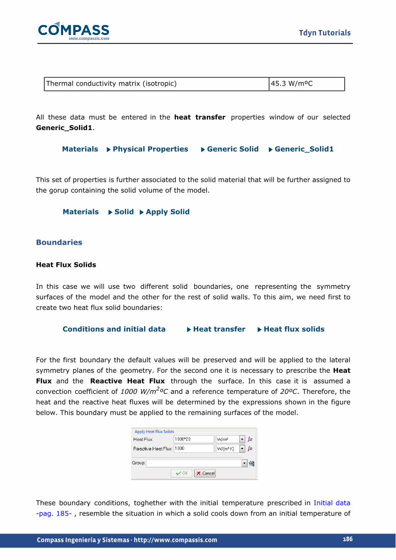
Tdyn Tutorials


Thermal conductivity matrix (isotropic) 45.3 W/mºC

All these data must be entered in the heat transfer properties window of our selected Generic_Solid1.

Materials Physical Properties Generic Solid Generic_Solid1

This set of properties is further associated to the solid material that will be further assigned to the gorup containing the solid volume of the model.

Materials Solid Apply Solid

Boundaries

Heat Flux Solids

In this case we will use two different solid boundaries, one representing the symmetry surfaces of the model and the other for the rest of solid walls. To this aim, we need first to create two heat flux solid boundaries:

Conditions and initial data Heat transfer Heat flux solids

For the first boundary the default values will be preserved and will be applied to the lateral symmetry planes of the geometry. For the second one it is necessary to prescribe the Heat Flux and the Reactive Heat Flux through the surface. In this case it is assumed a convection coefficient of 1000 W/m2ºC and a reference temperature of 20ºC. Therefore, the heat and the reactive heat fluxes will be determined by the expressions shown in the figure below. This boundary must be applied to the remaining surfaces of the model.

These boundary conditions, toghether with the initial temperature prescribed in Initial data -pag. 185- , resemble the situation in which a solid cools down from an initial temperature of

Tdyn Tutorials


100ºC to the temperature 20ºC of the surrounding media.

Remarks:

Convection heat tranfer may be simulated by inserting the function q + h·(Tm-To) in the field

Heat Flux, being q a defined heat flow, h the transmission coefficient and Tothe external

temperature. However it is recommended to split this flow in two terms, constant flow q +h·Tothat should be inserted in the Heat Flow field and the coefficient of the temperature

dependant term h, that should be entered in Reactive Heat Flux field.

Problem data

Other problem data must be entered in the Fluid Dyn. & Multi-phy. Data section of the data tree.

Number of steps 150

Time increment 1 s

Max. iterations 3

Initial steps 0


Output Step 10

Output Start 1

Mesh generation

As usual we will generate a 3D mesh by means of GiD's meshing capabilities.

Prior to mesh generation, the element's size on each geometrical entity should be defined in order to obtain an accurate discretization of the geometry. In this case it is recomended to use the By Chordal Error tool with the parameters indicated in the following figure:

Mesh Unstructured Sizes by chordal error

Tdyn Tutorials


Afterwards, the mesh will be generated automatically using a default element size of 8 and an unstructured size transition of 0.5. The outcome of the mesh generation process is an unstructured mesh, consisting of about 5214 nodes and 27706 tetrahedral elements.

Calculate


Post-processing


Some results from the analysis are shown below:

Tdyn Tutorials


Initial temperature field (t = 10s)

Temperature field after cooling (t = 150s)

Tdyn Tutorials


Towing analysis of a wigley hull

Introduction

This example shows the necessary steps for the towing analysis of the so-called Wigley hull, with a Froude number Fr = 0.316, using the NAVAL capabilities of the CompassFEM suite. This example corresponds to a non-viscous case for which the symmetry of the geometry has been taken into account to make the simulation easier.

The Wigley hull is a standard model for validating both experimental and numerical data. The geometry of this model can be seen in the following picture.

Wigley hull model geometry

A Wigley hull is created according to the following equation

y = B/2 (1-((2·x)/L)2)·(1-(z/D)2)

where L, D and B represent the length, draft and beam parameters respectively.

For the example to be solve here, the above parameters take the following values:

Length L 6 m

Beam B 0.6 m

Draft D 0.375 m

Since the Froude number is given by the following expression,

Tdyn Tutorials


Fn = v/√(g·L)

prescribing Fn = 0.316 results in a required analysis velocity of v = 2.424 m/s and a Reynolds number of Re = 1.5·107. Such a Reynolds number corresponds in fact to a fluid with a density ρ=1025 kg/m3 and a viscosity μ = 1.0·10-3 kg/m·s.

Start data


3D Flow in Fluids Transpiration

See the Start Data section of the Cavity flow problem (Start data -pag. 14-) for details on the Start Data window.

Pre-processing

The definition of the geometry is the first step to solve any problem.

Hull geometry definition

First, to create the hull we need to generate NURBS lines defining the different waterlines of the model. The hull itself will be constructed as a NURBS surface based on those previously generated lines. In the following paragraph we will show the necessary steps to create the hull using the pre-processor system.

The surfaces defining the hull will be created using a batch file. This batch file is just a text file (in ASCII format) containing the data points and the instructions listed in Appendix -pag. 209- . This set of instructions can be also inserted in the command line of GiD's pre-processor module. Once the batch file has been created (and saved in a text ASCII file), it can be read using the option Import->Batch file in the Files menu (or pressing Ctrl+B). By doing this, the following sequence of actions is done automatically:

Body_dry layer is created Two waterlines above the floating line are generated Free_surf layer is created The floating line is drawn A NURBS surface, describing the hull geometry above the floating line is created, based on the defined waterlines.

Tdyn Tutorials


Body_wet layer is created The waterlines below the floating line are generated A NURBS surface, describing the hull geometry below the floating line is created, based on the defined waterlines Auxiliary lines and points are deleted

The result of this process is shown in the figure below (i.e. half of the ship geometry since symmetry conditions are taken into account).

Hull geometry after execution of the batch file

Control volume definition

The analysis of hydrodynamic flows is done within the so-called control volume, which represents the volume of water around the model where the simulation is going to be carried on. Hence, after hull definition it is also necessary to define the geometry of the control volume. This is described next.

Definition of pointsThe eight necessary points to define the control volume around the ship hull have been selected by the following procedure and are listed in the table below. Note that it is not necessary to reproduce all the steps as the points are listed below and can be introduced by the standard procedure.

1) Identify the two extreme points of the floating line (intersection between the ship and the free surface of the water). These two points, which are placed in the bow and stern of the ship, will be hereafter named fore-point and aft-point respectively (the length of the ship is defined to be the distance from the fore to the aft point).

Tdyn Tutorials


2) Copy the fore-point to point A, which will be placed at 70% the ship length ahead (upstream) along (-) X-axis.

3) Copy point A to point B placed at 80% the ship length along (+)Y-axis.

4) Copy the aft-point to point C, which will be placed at 140% the ship length downstream along (+) X-axis.

5) Copy point C to point D placed at 80% the ship length along (+) Y-axis.

6) Copy points A, B, C and D 70% the ship length along (-) Z-axis to create points E, F, G and H.

Tdyn Tutorials


X Y Z X Y Z

Point A -7.2 0.0 0.0 Point E -7.2 0.0 -4.2

Point B -7.2 4.8 0.0 Point F -7.2 4.8 -4.2

Point C 11.4 0.0 0.0 Point G 11.4 0.0 -4.2

Point D 11.4 4.8 0.0 Point H 11.4 4.8 -4.2

Definition of the lines

The lines to be created have to join the following points A-B-C-D, E-F-G-H, A-E, B-F, C-G and D-H. Finally the points A and D have to be joint to the aft and fore-points respectively to obtain the sketch of the final geometry.

Definition of surfaces

The surfaces to be created are those defining the six faces of the box (control volume). These can be created following one of the standard procedures available in GiD pre-processor.

Definition of volumes

Wigley hull surfaces and those created in the previous step will define a single volume, which is the control volume of the present problem. To create the volume, use the following option of the Geometry menu:

Geometry Create Volume By contour

If the volume cannot be created for whatever reasons, check that all the surfaces were properly created, that there were no duplicated lines and that all the surfaces belong to a single and eventually closed volume. The resulting geometry is shown in the following figure.

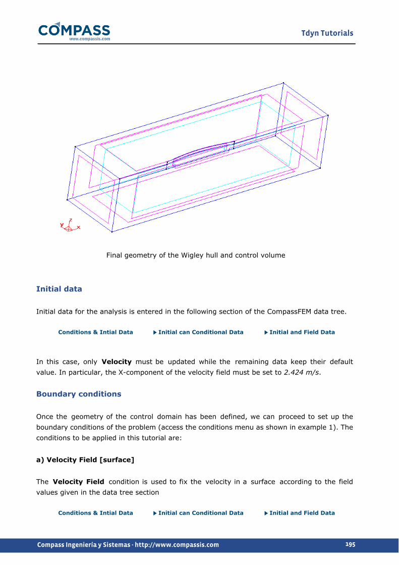
Tdyn Tutorials


Final geometry of the Wigley hull and control volume

Initial data

Initial data for the analysis is entered in the following section of the CompassFEM data tree.

Conditions & Intial Data Initial can Conditional Data Initial and Field Data

In this case, only Velocity must be updated while the remaining data keep their default value. In particular, the X-component of the velocity field must be set to 2.424 m/s.

Boundary conditions

Once the geometry of the control domain has been defined, we can proceed to set up the boundary conditions of the problem (access the conditions menu as shown in example 1). The conditions to be applied in this tutorial are:

a) Velocity Field [surface]

The Velocity Field condition is used to fix the velocity in a surface according to the field values given in the data tree section

Conditions & Intial Data Initial can Conditional Data Initial and Field Data

Tdyn Tutorials


In general these field values can be a function so that this condition can be used to specify a time or space dependant inflow condition. In order to do this, the corresponding Fix Field flag has to be marked. Alternatively, it is also possible to fix the velocity (during all the simulation process) to the initial value of the function given in the Initial and Field Data window. To do this, the corresponding Fix Initial flag has to be marked.

In this tutorial the Velocity Field boundary condition is going to be assigned to the inlet, lateral and bottom surfaces of the control volume. The activation flag options for each of the above-mentioned surfaces are shown in the figure below, while the actual field values can be checked in the Initial data -pag. 195- section.

Velocity Field activation flags for the inlet surface

Tdyn Tutorials


Velocity Field activation flags for the bottom surface

b) Pressure Field [surface]

Here we will apply a Pressure Field condition to the outlet surface of the domain. To this aim, it is necessary to mark the Fix Initial flag for the pressure field condition:

Conditions & Intial Data Initial can Conditional Data Pressure field

By doing this, the pressure in the outlet surface of the model will be fixed to the initial value of the function (in this case a constant zero value) given in the corresponding field of the initial data section.

Materials

Physical properties of the materials used in the problem (and some complex boundary conditions) are defined in the following section of the CompassFEM Data tree.


Some predefined materials already exist, while new material properties can be also defined if needed. In this case, only thermal properties are relevant for our solid material. These properties must be associated to the material assigned to the volumetric domain. This assignment is done using the following sequence in the data tree:

Tdyn Tutorials


Materials Fluid

The specific fluid property values of the material at hand are those listed in the following table.

Density 1025 kg/m3

Viscosity 1.0·10-3 kg/ms

All these data must be entered in the fluid flow properties window of our selected fluid.


This set of properties is further associated to the fluid material and assigned to the group containing the volume of the model.


Boundaries

Fluid Wall/Bodies

In this case only one fluid Wall condition is necessary. This must be assigned to the surface of the hull in contact with the fluid.

An ITTC Wall type will be assigned as the boundary type of the defined wall. An the corresponding law of the wall parameters are shown in the figure below.

Tdyn Tutorials


Wall properties assigned to the surface of the hull

It is important to remark that, in general, in free surface problems (but not in the present example) a control in the stern of bodies (in the transpiration problem) has to be carried on. This control would be applied in those points of the floating line of the body where the angle between the normal and the velocity is greater than SternC Angle. The recommended values for such a aparameter vary from 45º to 70º (see Reference Manual for further information).

Free surface

Finally, free surface properties must be prescribed for the top surface of the control volume. All data will keep their default values, except the Length parameter which will be set to the ship length value L=6.0 m (see figure below).

Tdyn Tutorials


Free surface window

Problem data

Other problem data must be entered in the Fluid Dyn. & Multi-phy. Data section of the data tree. For this example, the Fluid Flow and the Free Surface (transpiration) problems must be solved by using the following parameters:

Number of steps 600


Max. iterations 1

Initial steps 50


Output Step 50

Output Start 1

Remark: it is important to take in mind that the recommended value of the Time Increment for free surface analysis is dt<0.05L/Vor dt<h/V, being L a characteristic length, V the mean velocity, and h an average of the element size.

Write elevation option must be selected in the results section. YPlane Symm. in Fluid with 0.0 coordinate in the List of OY symm. planes corresponding field must be also used to account for the symmetry of the problem being modelled.

Tdyn Tutorials


For the simulation of Free Surface problems using the NAVAL module, it is also strongly recommended to define Initial Steps to be aproximatelly 5-10% the Number of Steps.

Modules data

Because of the conditions of the problem treated in this tutorial, turbulence effects will appear. Hence, a turbulence model to be used in the simulation must be especified:

Modules data Fluid flow Turbulence

In this case, the K Energy Two Layers model will be selected. Fix Turbulence on Bodies option may retain its delault value Auto. Such an option is accessible thorugh the following entry of the data tree:

Modules data Fluid flow Turbulence More... Fix Turbulence on Bodies

Mesh generation

The mesh to be used in the present analysis will be generated using linear tetrahedral elements.

Size assignment:

The size of the elements is of critical importance. Too big elements can lead to bad quality results, whereas too small elements can dramatically increase the computational time without improving the quality of the results. In this example the mesh size of the free surface (and also the lines and points contained on it) will be set to 0.1, while the points, lines and surfaces pertaining to the hull will be assigned a value 0.05.

After that, the mesh is generated selecting the corresponding option Mesh->Generate mesh in the main menu. On doing this, the elements general size must be fixed to 1.0 in the emerging window and an unstructured size transition of 0.4 must be specified.

The resulting mesh contains about 100.000 elements but is still too coarse for practical purposes. Nevertheless, it is enough for testing the capabilities of the program.

Calculate


Tdyn Tutorials


By using the Calculate window (accessible through the Calculate menu), it is also possible to start and manage the analysis of the problem.

Calculate window

Several analysis or processes can be run at the same time, and its management can be controlled using the calculate window shown in the previous figure. A list of all running processes is shown, with some usefull information like the project name, starting time, etc. Other options available are:

Start: begins the calculation. Once it is pressed, you can continue working with the pre-processor as usual.

Kill: after selecting a running process, this button stops its execution

Ouput view: after selecting a running process, this button opens a window that shows process related information as for instance the number of iterations, convergence information, etc.

Close: closes the window but does not stop the running processes.

When the calculation process is finished, the system displays the following message:

Process '...' started on ... has finished.

Then the results can be visualized by selecting activating the Postprocess module. Note that the intermediate results can be shown at any moment of the process even if the calculations are not finished yet.

Tdyn Tutorials


Post-processing

When the analysis is completed and the message Process '...' started on ... has finished. has been displayed, we can proceed to visualise the results by pressing Postprocess. For details on the result visualisation not explained here, please refer to the Post-processing chapter of the previous examples and to the GiD manual or GiD online help.

Inside the post-processing module, two main windows can be accessed in irder to make easier the visualization of the results. These windows are Select & Display Style and View Results.

Select and Display Style:

The Select & Display Style window allows the user to select which elements of the mesh and how they will be represented. This window allows selecting Materials (Volumes), Boundaries (Surfaces) and Cuts. Note that every material or boundary defined in the preprocessing part is shown in this window with the same name but with a prefix making reference to the type of geometrical entity (volume or surface).

The user can switch them On and Off by pressing the corresponding icon. Also, clicking on a set, and pressing Color the user can change the Ambient, Diffuse, Specular and Shininess component colour of the selected set, or give it its Default colour back.

Many other utilities are available in this window. For further information please consult the reference manual of the pre/postprocessing module.

View Results:

This window presents the results grouped into steps and allows the user to choose the result to be represented and the way this result will be displayed. The steps represent partial results in the convergence process of the problem. The user has to select which analysis and step is to be used for displaying results. The button Analysis Selection is used to select the module analysis (results are grouped depending on the different module problems available), and step to be used for the rest of the results options. If some of the results view requires another analysis or step, the user will be asked for it.

The View results window allows the access to the next display options: contour fill, contour lines, show minimum and maximum and display vector.

The Contour Fill option allows the visualisation of coloured zones, in which a variable, or a component, varies between two defined values. The contour line option is quite similar to contour fill, but here, the isolines of a certain nodal variable are drawn. In this case, each

Tdyn Tutorials


colour ties several points with the same value of the variable chosen. The Minimum and Maximum option allows seeing the minimum and maximum of the chosen result.

We can use View results window to see the velocity and pressure maps as shown in the figure below. To do it, select options as indicated here:

Analysis: RANSOL

Step: 90

View: Contour Fill

Results: PRESSURE


Analysis: RANSOL

Step: 90

View: Contour Fill

Results: VELOCITY

Tdyn Tutorials


Velocity distribution

Making graphs:

Graphs can be easily drawn using the View Graphs window (Window->View Graphs menu sequence). This window allows the user to select the variable and line (border) to define the graph.

As graphs are visualized over a cross section or boundary line only, we have to proceed by cutting the mesh at the desired position. To do a cut, use the Do Cuts->Cut Plane->2 points menu sequence. This option allows the definition of the cutting plane by giving 2 points (the cut plane will then be perpendicular to the view drawn on the screen).

In the present case, select View->Rotate->Plane XY (Original) to define the original view, and do a cut defined by the points (0.0, 1.0, 0.0) and (1.0, 1.0, 0.0). In the Select & Display Style window the new sets resulting from the cut will appear defined toghether with the other sets. Turn off all entities except the "CutSet FreeSurface" and select View Results->Default Analysis/Step->NAVAL->90 as the analysis step to be used for the graph visualization. Then, select Wave Elevation as the variable to be drawn in the View Graphs window, and X_Variation for the X-axis of the graph. Click Select Border button and select the only set that is visualized. Finally clcik on Actions button and select Draw Graphs to obtain the graph shown in the figure.

Tdyn Tutorials


Surface wave elevation along a longitudinal cut

Now, turn on the FreeSurface set in the Select & Display Style window, and repeat the process described above but selecting the border line of the free surface set. Then, you will be able to visualize the variation of the wave elevation on the border of this set, thus including the wave profile about the hull.

Surface wave elevation along the boundary of the free surface (including the ship hull)

Tdyn Tutorials


Finally, to check the quality of the obtained results, the calculated wave profile on the hull can be compared with experimental data. Such a comparison is shown in the figure below. As can be observed, both results are quite similar, although mesh refinement is necessary in the bow area to accurately capture the wave perturbation in that area.

Experimental vs. computed wave profile in the hull

Resistance results:

Data concerning forces acting on the hull can be accessed through the menu options View results->Forces on Boundaries, and View Results->Forces Graphs. Results from the simulation can be compared with the resistance values of the model, using the standard decomposition given by:

CT = CV + CW = (1+k)·Cf+CW

being CT the total resistance coeficient, CV=2.0·VFx/(ρ·S·v2) the viscous drag coeficient and

CW=2.0·P·Fx/(ρ·S·v2) the wave resistance coefficient. Herein ρ is is the fluid densisty, S is the

wetted area and v the velocity of the analysis.

We can evaluate the viscous drag coeficient from:

Cv = (1+k)*0.075/(log10(Re)-2)2

Tdyn Tutorials


Experimentally, a value of k ≈ 0.09 is obtained, and since Re = ρ·v·L/μ = 1.45·107, we can estimate Cv = 3.07·10-3, while the result from our simulation is Cv = 2.90·10-3. The

experimental data for the wave drag Cw ≈ 1.5·10-3can be compared with the pressure force

obtained in the simulation Cw = 1.4·10-3. As can be seen, both values are quite similar to the

experimental ones.

Such a comparison must be considered as an approximation, since the two force components obtained through the simulation do not exactly correspond to the theoretical values.

Tdyn Tutorials


Appendix

escape escape escapeview layers new body_dryescape escape escapegeometry create nurbslineescape create nurbsline-3.0000 0.0000 0.2000-2.5000 0.0917 0.2000-2.0000 0.1667 0.2000-1.5000 0.2250 0.2000-1.0000 0.2667 0.2000-0.5000 0.2917 0.20000.0000 0.3000 0.20000.5000 0.2917 0.20001.0000 0.2667 0.20001.5000 0.2250 0.20002.0000 0.1667 0.20002.5000 0.0917 0.20003.0000 0.0000 0.2000escape create nurbsline-3.0000 0.0000 0.0500-2.5000 0.0917 0.0500-2.0000 0.1667 0.0500-1.5000 0.2250 0.0500-1.0000 0.2667 0.0500-0.5000 0.2917 0.05000.0000 0.3000 0.05000.5000 0.2917 0.05001.0000 0.2667 0.05001.5000 0.2250 0.05002.0000 0.1667 0.0500

Tdyn Tutorials


2.5000 0.0917 0.05003.0000 0.0000 0.0500escape escape escapeview layers new free_surfescape escape escapegeometry create nurbslineescape create nurbsline-3.0000 0.0000 0.0000-2.5000 0.0917 0.0000-2.0000 0.1667 0.0000-1.5000 0.2250 0.0000-1.0000 0.2667 0.0000-0.5000 0.2917 0.00000.0000 0.3000 0.00000.5000 0.2917 0.00001.0000 0.2667 0.00001.5000 0.2250 0.00002.0000 0.1667 0.00002.5000 0.0917 0.00003.0000 0.0000 0.0000escape escape escapeview layers touse body_dry escape escape escapegeometry create nurbssurface parallellines layer:body_dry layer:free_surfescape escape escapeview layers new body_wetescape escape escapegeometry create nurbsline-3.0000 0.0000 -0.0500-2.5000 0.0900 -0.0500-2.0000 0.1637 -0.0500-1.5000 0.2210 -0.0500

Tdyn Tutorials


-1.0000 0.2619 -0.0500-0.5000 0.2865 -0.05000.0000 0.2947 -0.05000.5000 0.2865 -0.05001.0000 0.2619 -0.05001.5000 0.2210 -0.05002.0000 0.1637 -0.05002.5000 0.0900 -0.05003.0000 0.0000 -0.0500escape create nurbsline-3.0000 0.0000 -0.1000-2.5000 0.0851 -0.1000-2.0000 0.1548 -0.1000-1.5000 0.2090 -0.1000-1.0000 0.2477 -0.1000-0.5000 0.2709 -0.10000.0000 0.2787 -0.10000.5000 0.2709 -0.10001.0000 0.2477 -0.10001.5000 0.2090 -0.10002.0000 0.1548 -0.10002.5000 0.0851 -0.10003.0000 0.0000 -0.1000escape create nurbsline-3.0000 0.0000 -0.1500-2.5000 0.0770 -0.1500-2.0000 0.1400 -0.1500-1.5000 0.1890 -0.1500-1.0000 0.2240 -0.1500-0.5000 0.2450 -0.15000.0000 0.2520 -0.15000.5000 0.2450 -0.1500

Tdyn Tutorials


1.0000 0.2240 -0.15001.5000 0.1890 -0.15002.0000 0.1400 -0.15002.5000 0.0770 -0.15003.0000 0.0000 -0.1500escape create nurbsline-3.0000 0.0000 -0.2000-2.5000 0.0656 -0.2000-2.0000 0.1193 -0.2000-1.5000 0.1610 -0.2000-1.0000 0.1908 -0.2000-0.5000 0.2087 -0.20000.0000 0.2147 -0.20000.5000 0.2087 -0.20001.0000 0.1908 -0.20001.5000 0.1610 -0.20002.0000 0.1193 -0.20002.5000 0.0656 -0.20003.0000 0.0000 -0.2000escape create nurbsline-3.0000 0.0000 -0.2500-2.5000 0.0509 -0.2500-2.0000 0.0926 -0.2500-1.5000 0.1250 -0.2500-1.0000 0.1481 -0.2500-0.5000 0.1620 -0.25000.0000 0.1667 -0.25000.5000 0.1620 -0.25001.0000 0.1481 -0.25001.5000 0.1250 -0.25002.0000 0.0926 -0.25002.5000 0.0509 -0.2500

Tdyn Tutorials


3.0000 0.0000 -0.2500escape create nurbsline-3.0000 0.0000 -0.3000-2.5000 0.0330 -0.3000-2.0000 0.0600 -0.3000-1.5000 0.0810 -0.3000-1.0000 0.0960 -0.3000-0.5000 0.1050 -0.30000.0000 0.1080 -0.30000.5000 0.1050 -0.30001.0000 0.0960 -0.30001.5000 0.0810 -0.30002.0000 0.0600 -0.30002.5000 0.0330 -0.30003.0000 0.0000 -0.3000escape create nurbsline-3.0000 0.0000 -0.3750-2.5000 0.0000 -0.3750-2.0000 0.0000 -0.3750-1.5000 0.0000 -0.3750-1.0000 0.0000 -0.3750-0.5000 0.0000 -0.37500.0000 0.0000 -0.37500.5000 0.0000 -0.37501.0000 0.0000 -0.37501.5000 0.0000 -0.37502.0000 0.0000 -0.37502.5000 0.0000 -0.37503.0000 0.0000 -0.3750escape escape escapeview layers touse body_wetescape escape escape

Tdyn Tutorials


geometry create nurbssurface parallellines layer:body_wet layer:free_surfescape escape escapegeometry delete line layer:body_wet escape escapegeometry delete point layer:body_wet escape escapegeometry delete line layer:body_dry escape escapegeometry delete point layer:body_dry escape escapeescape escape escape

Tdyn Tutorials


Wigley hull in head waves

Introduction

This example illustrates the analysis of a Wigley hull in head waves using ODDLS module. The analysis will be carried out with the ship moving forward with a Froude number Fr = 0.316.

Result of the analysis of the Wigley hull in head waves

Start data

For this example, the following selection has to be done in the Start Data window of the CompassFEM suite.

3DFlow in FluidsMesh deformationOdd Level Set

The rest of the data remains the same.

See the Start data -pag. 14- section for further information on the Start Data window.

Pre-processing

Hull geometry definition

Tdyn Tutorials


The hull geometry to be used in this example will be generated in a similar way to the previous case. However, in this case the script to be used has been modified to extend the depht of the ship. The mentioned script can be found here Appendix -pag. 224-.

Once the geometry of the ship has been generated, it has to be mirrowed, since for this example the total geometry will be used.

Control volume definition

The control volume for the example will be generated using the following process. Note that in this case, two volumes will be generated, one for the initial water volume and other for the initial air volume.

1 Create the points of the bottom surface, listed below.

x y z

-7.5 6.0 -3.0

-7.5 -6.0 -3.0

12.0 -6.0 -3.0

12.0 6.0 -3.0

2 Join the new points by creating the four boundary lines of the bottom surface.3 Copy the new lines using the copy tool at z=0.0 and z=1.5.4 Create the boundary surfaces of the volume and the initial (still) free surface.5 Generate the volumes defined by the different surfaces.

The resulting volume is shown in the following picture:

Tdyn Tutorials


Control volume for the analysis of a Wigley hull in head waves

Problem data

Several problem data must be entered in the Fluid Dyn. & Multi-phy. Data section of the data tree. For this example, the following parameters have to be modified:

Fluid Dyn. & Multi-phy. Data Analysis

Number of steps 600


Max. iterations 1

Initial steps 0

Remark:

In this example, the Time Increment has been selected as dt=0.02·L/V, being L a characteristic length, V the mean velocity, and h an average of the element size.

Fluid Dyn. & Multi-phy. Data Results

Output Step 15

Tdyn Tutorials


Output Start 1

Fluid Dyn. & Multi-phy. Data Other

Press. Ref. Location Yes

Orig. X val 0.0 m

Orig. Y val 0.0 m

Orig. Z val 0.0 m

YPlane Symm. in Fluid Yes

List of OY symm. planes 6.0,-6.0

ZPlane Symm. in Fluid Yes

List of OZ symm. planes 1.5,-3.0

Remark:

The pressure reference for the hydrostatic component of the pressure is set to the initial position of the free surface.

The different symmetry planes allow to easily apply boundary conditions to the boundaries of the control volume.

Modules data

Fluid Flow data

Since we are imposing transient boundary conditions, it is advisable to set Press. Inner Iter. to 2.

Modules Data Fluid Flow General Pressure Inner Iterations

This will increase the iterations of the pressure solver and therefore the precision of the results.

Because of the conditions of the problem treated in this tutorial, turbulence effects will appear. The turbulence model to be used in the simulation (Spalart-Allmaras model) will be specified in

Tdyn Tutorials


Modules Data Fluid Flow Turbulence

The rest of data remain the same.

Free Surface (ODDLS) data

The solver scheme has to be set to ODD Level Set. The rest of data remain the same.

Initial data

Initial data for the analysis will be entered in the following data section of the CompassFEM data tree

Conditions & Initial Data Initial and Field Data

In this example, the X-component of the velocity field (Velocity X Field) must be set to 2.424 m/s, while the initial eddy kinetic energy (k, EddyKEner Field) has to be set to 0.00088 m2/s2 and the characteristic eddy length (L, Eddy Length Field) will be set to 1.68·10-5 m.

The last two values has been calculated, taken a TIL (turbulence intensity level) of 1% and an initial ratio between eddy viscosity and physical viscosity (μT/μ) of 0.5. Therefore:

k=3/2·(TIL·V)2=0.00088 m2/s2

V=√k=0.0297 m/s

L=μT/(ρ·V)=1.684·10-5 m

Furthermore, the level set function must be initiated, defining the initial position of the free surface.

Conditions & Initial Data Initial and Field Data OddLevelSet Field

In this case, OddLevelSet Field will be specified by the following function:

lindelta(-z,0.5)

The second argument of the lindelta function must be of the order of four times the characteristic element size at the free surface.

Tdyn Tutorials


Boundaries

Now, it is necessary to set the boundary conditions of the problem. The different conditions to be defined are shown next.


In this case, the inlet condition will simulate a wave generator. A new Inlet group will be created with Inlet Velc as boundary type. The inlet condition will be assigned to the two inlet surfaces of the control volume.

The waves will be created by defining an oscillating velocity given by Vel X Field = 2.424+0.6*sin(3.66*t). The frequency of the wave generator oscillation corresponds to the relative wave frequency.

Conditions & Initial Data Fluid Flow Outlet

A new outlet group will be created and applied to the two outlet surfaces of the control volume. The Outlet type used in this case will be OutletPres (a null dynamic pressure will be applied).


Finally, the ship has to be identified as a body. A new group Ship will be created with YplusWall as boundary type and a Yplus value of 65. The condition will be applied to all the surfaces of the ship.

Furthermore, the Estimate Body Mass option has to selected and the OY Radius of gyration set to 2.1 m (35% of the length of the ship). The Z Displacement and OY Rotation will be set to free to allow those movements of the ship.

Tdyn Tutorials


Inlet, Outlet and Ship boundary conditions.

Conditions & Initial Data Mesh Deformation Fix Mesh Deformation

Since the calculation includes the automatic adaptation (deformation) of the mesh, following the movement of the ship, the mesh movement has to be fixed somewhere.

In this case, the mesh deformation has to be null (Fix Null) in the boundary surfaces shown in the following picture.

Tdyn Tutorials


Fix Mesh deformation condition.

Conditions & Initial Data Free Surface (ODDLS) ODDLS Field Fix Field

Finally, the resolution of the level set equation requires some boundary conditions. In this case, the inlet surfaces will be set to the field value of the level set. This implies to activate the Fix Field option.

Materials

Physical properties of the materials used in the problem (and some complex boundary conditions) are defined in the following section of the CompassFEM data tree

Materials PhysicalProperties

For this example, we will create a new Generic Fluid, that we will rename as "My Fluid" with the following physical properties:

Density 1000 kg/m3

Viscosity 1.0·10-3 kg/ms

Furthermore, we need to add an absorbing boundary condition to the model, to avoid any reflection of the generated waves on the outlet. The easiest way to do this is by creating a damping area (beach) for the waves. For this purpose an Acceleration Field will be defined using the following functions:

Materials PhysicalProperties Generic Fluid My Fluid Fluid Flow Acceleration Field

Component X:

if(x>=9)then(-0.05*(vx-2.424)/dt)else(0)endif

Component Y:

if(x>=9)then(-0.05*vy/dt)else(0)endif

Component Z:

if(x>=9)then(-0.05*vz/dt)else(0)endif

Tdyn Tutorials


Finally, the new material has to be assigned to the control volume.

Mesh generation

An element size of 0.05 m has been assigned to the hull surfaces, lines and points. The same element size has been assigned to the surface (lines and points) between the two volumes, representing the initial free surface.

The resulting mesh, using a size transition of 0.4 and a maximum element size of 0.3 m has about 315 000 linear tetrahedra.

Calculate

The calculation process will be started through the Calculate menu, as in the previous examples.

Post-processing

Since the analysis has been carried out with an automatic mesh adaptation, in order to correctly visualise the results, it is necessary to apply the corresponding mesh deformation for every time step. This can be achieved by activating the Draw Deformed option in the postprocess data tree (see Postprocess reference manual for further details).

Probably, the best way to visualize the free surface interacting with the hull is with the isosurfaces visualization options. To this aim, create an isosurface corresponding to a value of 0.5 of the ODDLS variable.

Next figure shows a sequence of the free surface results obtained in this example.

Tdyn Tutorials


For details on the results visualisation not explained here, please refer to the Post-processing chapter of the previous examples and to the Postprocess reference manual.

Appendix

The same type of script as in the previous example is used in the present case to automatically generate the geometry of the hull. See section Appendix -pag. 209-. However, in this case the script to be used must be modified to extend the depht of the ship. Actually, the first nurbsline created in the script of section Appendix -pag. 209- must be substituted by the following code so that z-coordinate changes from 0.25 to 0.75.

...

escape create nurbsline-3.0000 0.0000 0.7500-2.5000 0.0917 0.7500-2.0000 0.1667 0.7500-1.5000 0.2250 0.7500-1.0000 0.2667 0.7500-0.5000 0.2917 0.75000.0000 0.3000 0.75000.5000 0.2917 0.75001.0000 0.2667 0.7500

Tdyn Tutorials


1.5000 0.2250 0.75002.0000 0.1667 0.75002.5000 0.0917 0.75003.0000 0.0000 0.7500escape create nurbsline...

Thermal contact between two solids

Introduction

This tutorial concerns the heat transfer problem between two solid boxes in contact.

Start data




Pre-processing

The geometry of the present problem simply consists of two square boxes representing the solids in contact. The easiest way to generate the geometry is to copy the existing one in 3D Cavity flow -pag. 115-. When doing the copy of the original box, do not forget to select the option Duplicate entities in the Copy window.

Tdyn Tutorials


Boundary conditions

Once the geometry of the control domain has been defined, we can proceed to set up the boundary conditions of the problem (access the conditions menu as shown in example 1). The only conditions to be applied in this example correspond to the Fix Temperature condition (Conds. & Init. Data->Heat Transfer->Fix Temperature) that must be applied to the opposite edges of the two solids in contact.

Conditions and Initial data Heat transfer Fix temperature

Therefore, the temperature of the top right corner edge of the first solid must be fixed to 100ºC, while the temperature of the bottom left edge of the second solid must be fixed to 0ºC.

Materials

Physical properties of the materials used in the problem (and some complex boundary conditions) are defined in the section Physical properties section of the Materials data in the tree. Some predefined materials already exist, while new material properties can be also defined if needed. In this case, only thermal properties are relevant for our solid material.

In this simple example the thermal properties of both solids are taken to be identical. Therefore, only one set of thermal properties must be defined and assigned to both volumes in the model. The default existing Generic_Solid can be reused so that only the specific heat

Tdyn Tutorials


must be modified from its default value.

Thermal properties to be used are summarized here:

Density 1 kg/m3

Specific heat 10 J/kg·K

Thermal conductivity matrix 1 W/m·K

Contacts

Next, we must define the contact between the solid.

Solid-Solid contact (SSContact):

SSContact boundaries identify a contact with continuity of the corresponding fields between two solid domains. We will use this boundary to define the continuity of the temperature field through the two central (contact) surfaces. The SSContact boundary can be applied in the Contacts section of the CompassFEMFD&M data tree. Analogously, FFContacts could be used

to create a contact with continuity in the selected fields between two fluid domains and FSContacts to create a contact with continuity in the selected fields between a fluid and a solid domain.

In the present case, only temperature field continuity through the contact surface must be ensured, since the fluid flow problem is not solved. Hence, only heat transfer contact properties need to be set as shown in the figure below.

Contacts Contacts CFD Solid-Solid contacts Heat transfer

Finally, contact properties must be assigned to the central (contacting) surfaces of the model

Tdyn Tutorials


geometry as shown in the following figure. Note that, by contrast to the Fluid-Solid Contact described in Fluid-Solid thermal contact -pag. 84-, the Solid-Solid SContact and Fluid-Fluid Contact cases require the contacting surfaces of the two domains to be identified and assigned separately (Assign Side A and Assign Side B options). The easiest way to proceed is by sending each one of the volumes and their attached lower entities to separate layers (use the tools available in Utilities->Layers window of the preprocessor). Switch on/off the two layers alternatively and assign sides A and B to each one of the corresponding contact surfaces. Please refer to the GiD User Manual for further information about how to work with layers.

Solid-Solid contact side A assignement

Tdyn Tutorials


Solid-Solid contact Side B assignement

Problem data

Once the boundary conditions have been assigned and the materials have been defined, we have to specify the other parameters of the problem. The values listed next have to be entered in the Problem and Analysis pages of the Fluid Dyn. & Multi-phy. Data section of the data tree.

Problem->Solve Fluid


Solve Heat transfer 0 (NO)

Problem->Solve Solid



Analysis

Number of Steps 1

Time increment infinite

Max iterations 1

Initial steps 0

Tdyn Tutorials



Mesh generation

The mesh to be used in this example will be generated by defining a structured mesh of hexahedral elements in the right hand side box and an unstructured tetrahedral mesh in the left hand side box. The structured mesh can be generated by using the menu option Mesh->Structured->Volume and selecting the corresponding volume entity. The number of cells to be assigned to all lines of thise volume will be 15.

Before generating the mesh, set to None the option Automatic correct sizes in the Meshing page of the Utilities->Preferences window.

Finally, the mesh can be generated using a maximum element size of 0.05. The resulting mesh consists of about 89000 elements and 19000 nodes.

Calculate

The calculation process will be started from within GiD through the Calculate menu, as in the previous examples.

Post-processing


The results shown in the following figure correspond to the steady state temperature distribution.

Tdyn Tutorials


Steady state temperature distribution

Tdyn Tutorials


Fluid-Structure interaction

Introduction

Tdyn offers the possibility to simulate coupled fluid-structure interaction problems, modelling fluid flow by the Navier-Stokes equations ans structural mechanics by the structural equation of motion. This tutorial illustrates the fluid-structure interaction capabilities of Tdyn for the particular case of a 3D flexible solid structure in a channel with a gradual contraction.

Start data

For fluid-structure interaction (FSI) problems, simulation type in the Start Data window must be set to Coupled Fluid-Structural Analysis.

In this case, the following type of problems must be loaded in the Start Data window.

3D Flow in Fluids Internal (coupling) Solids Dynamic: Direct Integration Analysis Linear Materials Mesh deformation

Note: in this tutorial, FSI concerns the transfer of fluid flow traction results to the structural solver. These traction results act then as the structural load over the solid structure. Although fluid domain mesh deformation, due to the movement of the solid structure, is not actually solve in this example, Mesh deformation option must be activated to allow the definition of fluid-solid coupling interfaces.

See the Start Data section of previous tutorials for details on the Start Data window.

Pre-processing

When performing coupled fluid-structure analyses, pertinent geometries must be created using the pre-processor, to represent fluid and structural domains. Both domains must be modelled by completely independent geometries. That means that no geometric object (point, line, surface or volume) that belong to the fluid domain may belong to any geometric object of the structural domain and vice versa. An useful approach to distinguish between geometric objects of the fluid and structural domains is to group them into different layers (see picture below).

Tdyn Tutorials


The model of the present problem consists of a channel with a gradual contraction. Right before the contraction there is a flexible solid flap.

First we should proceed to construct the fluid domain. The corresponding geometry and dimensions are shown in the following sketch (geometric units in meters). As can be observed, there is just one volume in the fluid. Such a volume is delimited by the channel and the flap surfaces.

Geometry of the fluid domain that includes the channel and the contour of the solid flap.

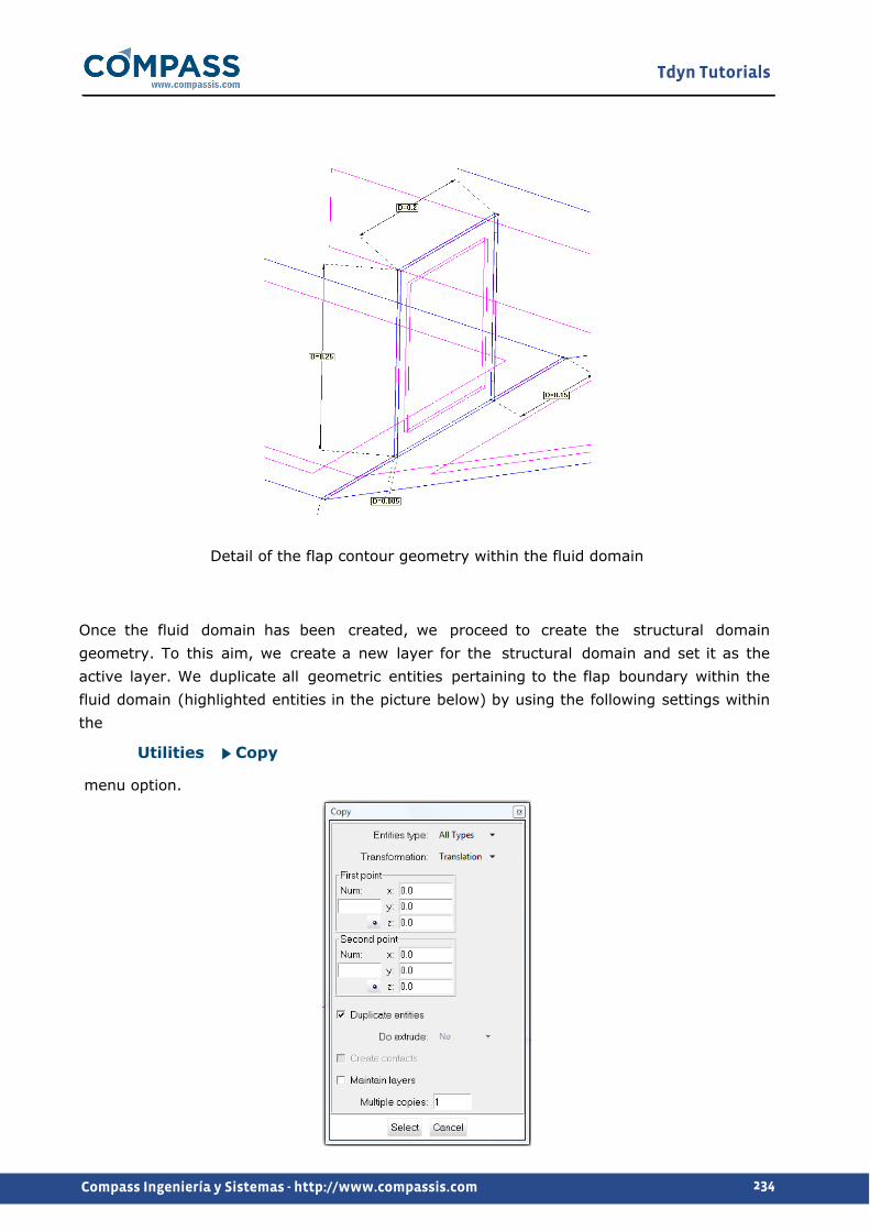
Tdyn Tutorials


Detail of the flap contour geometry within the fluid domain

Once the fluid domain has been created, we proceed to create the structural domain geometry. To this aim, we create a new layer for the structural domain and set it as the active layer. We duplicate all geometric entities pertaining to the flap boundary within the fluid domain (highlighted entities in the picture below) by using the following settings within the

Utilities Copy

menu option.

Tdyn Tutorials


Settings for entities duplication

Fluid domain entities selected to be duplicated

In order to provide a closed boundary for the solid flap, an additional surface must be created from the corresponding contour lines at the bottom of the structural domain. Finally, the volume for the flexible solid flap can be created from the six contour surfaces existing within the solid domain.

Tdyn Tutorials


Structural domain

General data

Some general information of the problem must be specified in

General Data

section of the data tree.

In particular, some general data concerning the structural part of the problem must be entered in

General Data Analysis

. The following are the pertinent settings for the present case.

Simulation Dimension: 3DProblem type: SolidsAnalysis type: Linear dynamicBeam P-Delta: 0

When Linear dynamic analysis type is activated, the section

General Data Linear dynamic General

becomes available also in the data tree. The following are the corresponding settings for the present problem.

Tdyn Tutorials


Type: Direct integrationIntegration method: Implicit

The remaining parameters within this section can retain the default value. Note that the time increment Δt and the number of steps is not active since the corresponding values are internally fixed according to the coupling data to be defined in

Coupling Data

section (Coupling data -pag. 237-).

Some additional information concerning the output of the structural problem may be also entered. The corresponding options will be detailed later in Problem data -pag. 243-.

Coupling data

Few general coupling parameters must be entered in the Coupling data section of the data tree. These are as follows:

Coupling type: internal Δt: 0.05 s Number of steps: 2000

The total number of steps and the time increment introduced herein automatically determine the number of steps and the time increment that will be used to solve the structural and fluid problems.

Boundary conditions

Once the geometries of fluid and solid domains have been defined, we can proceed to set up the boundary conditions of the problem.

Initial and Field Data

First, some fields that will be used to prescribe boundary conditions in fluid domain must be specified. For the present problem, the following inflow velocity will be used:

V(t) = Vmax/2 (1-cos(2π·t/10)) if t<10

V(t) = Vmax if t>10

where Vmax = 0.06067 m/s.

Hence, the following expression must be introduced in the function editor window

Tdyn Tutorials


corresponding to the Velocity X field in the data tree section

Conds. & Init. Data Initial and Field

.

if(t<=10)then(0.06067*0.5*(1-cos(pi*t/10)))else(0.06067)endif

Fluid Flow

All boundary conditions described here refer to the fluid domain. The user must ensure that these conditions are correctly applied to fluid domain entities. Hence, it is recommended to deactivate all layers containing solid domain entities to avoid their accidental selection.

Velocity Field (

Conds. & Init. Data Fluid Flow Velocity Field

): in the fluid domain, three different velocity field conditions will be applied to the inlet, lateral and upper surfaces of the channel respectively.

The three components of the velocity must be fixed in the inlet surface of the channel. Hence, X, Y and Z Fix Field flags must be activated in the Velocity Field condition and applied to the left surface of the fluid domain. The velocity component perpendicular to the lateral surfaces of the channel must be null. Hence, the Z Fix Initial flag must be activated in a new Velocity Field condition and applied to the lateral surfaces of the fluid domain. Finally, the vertical component of the velocity must be null on the upper surface of the channel. Hence, the Y Fix Initial flag must be activated in a new Velocity Field condition and applied to the upper surface of the fluid domain.

Pressure Field (

Conds. & Init. Data Fluid Flow Pressure Field

): in the fluid domain, pressure must be prescribed in the outlet surface of the channel. Hence, Fix Initial flag must be activated in the Pressure Field condition and applied to the surface on the right side of the fluid domain.

Wall/Bodies (


): a Wall/Body condition must be applied to the bottom surface of the channel and to the solid flap boundaries within the fluid domain. For the present case, a Yplus law of the wall type of boundary must be used on this Wall/Body condition. Open the


Tdyn Tutorials


option in the data tree and select Fluid Wall and Yplus Wall type inside the wall type tab. Further apply this condition to the surfaces shown in the figure below.

Assignement of Wall/Body condition to surface entities within the fluid domain

In order for the fluid-structure coupling to be effective, the Shell Coupling option must be activated in the motions tab of the Wall/Body condition.

Structural

Boundary conditions described here refer to the structural domain. The user must ensure that these conditions are correctly applied to structural domain entities. Hence, it is recommended to deactivate all layers containing fluid domain entities.

Fixed constraints (

Conds. & Init. Data Structural Fixed constraints

): the only structural boundary condition necessary for the present case is a Fixed constraints condition that must be applied to the bottom surface of the solid flap. Select

Conds. & Init. Data Structural Fixed constraints

and activate X, Y and Z Constraint options within the activation tab. The corresponding values within the values tab must remain equal to zero in order to fix all nodes located at the bottom surface of the flap structure.

Materials

Tdyn Tutorials


Physical properties of the materials used in the problem (and some complex boundary conditions) are defined in the section


of the data tree. Some predefined materials already exist, while new material properties can be also defined if needed. In this case, fluid material properties must be applied to the volume entity within the fluid domain, and solid material properties should be assigned to the volume entity within the structural domain.

Fluid physical properties.

In the data tree, right-click on

Materials Physical Properties Generic Fluid

option and select Create new material in the pop-up menu. Rename the new material to Silicon_Oil and open it to edit the corresponding fluid properties. Fluid flow properties must be set as follows:

Fluid Model: incompressible Density: 956 kg/m3

Viscosity: 0.145 kg/(m·s)

Finally, open the

Materials Fluid

option in the data tree, select Silicon_Oil in the materials list and apply it to the fluid domain volume.

Solid physical properties

In the data tree, right-click on

Materials Physical Properties Generic Solid

option and select Create new material in the pop-up menu. Rename the new material to User_generic_solid and open it to edit the corresponding structural properties. Elastic properties within the structural tab must be set as follows:

E: 2.3e6 Pa v: 0.45 Specific weight: 17400 N/m3

Finally, open the

Materials Solid

Tdyn Tutorials


option in the data tree, select User_generic_solid in the materials list and apply it to the structural domain volume.

Structural loads

In the present case, the load acting over the flap structure is originated by the traction field created by the passing fluid. Hence, the fluid-structure interaction is actually specified in this section through the definition of a coupling load. In this way, traction variable results from the fluid solver will be transferred and applied as a structural load over the boundaries of the flexible solid flap.

Coupling load:

Open the Structural loads Loadcase 1 Solids Pressure Load

option in the data tree.

In the Apply Pressure Load window select the Create/edit a function option next to the Factor field. A Create function for Factor window will appear. Activate the Function on time option and select Coupled load type. Since internal coupling was defined in Coupling data -pag. 237- only TCP/IP coupling option is available. Activate the TCP/IP coupling option and select RANSOL analysis type and Traction results option.Initial time for coupling can be set to 25, so that fluid-structure interaction will actually start in this case when the fluid flow has already stabilized. Send deformation must be set to no because mesh nodes displacement results are not transferred from the structural solver to the fluid domain in this case.

Tdyn Tutorials


Coupling settings

After pushing the OK button, Load type variable in the Apply Pressure Load window has been automatically set to local. All surface entities to which the coupling pressure load will be applied need to have local axes associated. To this aim, open the Apply or draw local axes option next to the Load type field. The following window will appear.

Select Assign automatic option and apply it to all surface entities of the structural domain that are in contact with the fluid.

Tdyn Tutorials


Finally, assign the already defined coupling load to all boundaries of the flap that are in contact with the fluid. To be sure that both, local axes and the coupling load are correctly assigned to structural entities, it would be useful to deactivate fluid domain layers during the assignment process.

Problem data

Once boundary conditions, materials and structural loads have been defined, additional general information must be introduced to solve the problem.

Fluid problem data:

In

Fluid Dyn. & Multi-phy. Data Problem Solve Fluid

only SOLVE FLUID, Solve Fluid Flow and Solve Mesh deformation options should be active (the corresponding field value must be equal 1).

In

Fluid Dyn. & Multi-phy. Data Problem Solve Solid

all options may be deactivated (the corresponding field value equal to 0) since no solid domain exist within the fluid part of the problem.

Fluid analysis data:

The following are the pertinent settings to be introduced in


for the present problem:

Max Iterations: 1Initial Steps: 0Steady State Solver: Off

The remaining parameters may retain their default value. Note that Number of Steps and Time Increment are automatically fixed according to

Coupling data

information.

Fluid results data:

The following are the values to be introduced in


Tdyn Tutorials


.

Output Step: 25Output Start: 500Result File: Binary

At least velocity and pressure variables should be activated in the output variables list in

Fluid Dyn. & Multi-phy. data Results Fluid Flow

. Mesh deformation variables can be deactivated in

Fluid Dyn. & Multi-phy. data Results Mesh Deformation

since the corresponding problem is not actually solved in the present case. Nevertheless, the mesh deformation type of problem must be selected in the Start Data window to provide fluid-solid coupling capabilities.

Structural problem data:

General structural problem data has been already defined in General data -pag. 236-. Furthermore, specific information concerning the output of the structural part of the problem may be introduced in

General Data Results Structural Analysis

and

General Data Advanced

. In particular, we can modify the output frequency for the structural problem setting the output step equal to 25 in

General Data Advanced Dynamic Output Output step

.

Mesh generation

Structural part mesh:

In order to mesh the structural part it is recommended to turn-off all layers containing fluid domain entities.

First, select structured mesh properties through the menu option Mesh Structured Volumes Assign number of cells

and apply it to the structural domain volume entity.

When asked for the number of cells to assign to lines introduce a value of 30 and apply it to the top and bottom lines of the structural part geometry. Repeat the procedure and

Tdyn Tutorials


assign 35 divisions to the right and left vertical lines, and 4 divisions to the through-thickness line entities (see picture below).

Next, assign type of elements to the volume and surface entities of the structural part. Hexahedra may be assigned to the volume by using the menu option

Mesh Element type Hexahedra

. Similarly, quadrilateral elements may be assigned to all surfaces of the flap.

To succesfully run fluid-structure interaction problems it is mandatory to leave the surface entities of the structural domain without meshing. Hence, the option

Mesh Mesh criteria No mesh Surfaces

must be applied to the structural domain surfaces. On the contrary, all surfaces of the fluid domain should be meshed.

Tdyn Tutorials


Fluid part mesh:

In order to mesh the fluid part, it is recommended to turn-off all layers containing structural domain entities. The fluid part is meshed with tetrahedrons using unstructured surfaces and volume meshes.

First, assign an element size of 0.025 to all external lines of the fluid domain by using the menu option

Mesh Unstructured Assign sizes on lines

. By the same procedure, assign an element size of 0.00125 to all internal lines of the fluid domain including the lines bounding the flap (see picture below).

Next, assign element sizes to the surface of the fluid domain by using the option Mesh Unstructured Assign element sizes to surfaces

. An element size of 0.00125 must be assigned to all through-thickness surfaces bounding th flap and the adjacent ones at the bottom of the channel. Sizes of 0.007 and 0.025 must be finally applied to both faces of the flap and to the external surfaces of the channel respectively.

Finally, apply an element size of 0.035 to the fluid domain volume by using the option Mesh Unstructured Assign sizes on volumes

.

Mesh is finally generated by using a maximum element size of 0.035 and an element transition of 0.2 in the Generate mesh window

Mesh Generate mesh

Tdyn Tutorials


.

The resulting mesh contains a total number of 413797 elements and 79724 nodes.

Calculate


Post-processing


In the following pictures the steady-state pressure and velocity fields are presented. The last picture shows the displacement of the flexible flap and the von Mises stress distribution within the solid.


Tdyn Tutorials


Velocity modulus distribution

Deformation of the flexible flap structure and von Misses stress distribution

Tdyn Tutorials


Potential flow with free surface

Introduction

This example shows the necessary steps to analyse the potential flow about a cylinder with linear free surface condition. The formulation of the free surface condition will be done using TdynTcl extension available in URSOLVER module.

Problem formulation

In the case of an incompressible flow the velocity potential satisfies Laplace's equation:

∇·(∇Φ)=0

Where Φ is the velocity potential, describing the velocity field as:

v=∇Φ

The FEM weak formulation of the potential flow problem can be written as follows:

∫Ω∇NiNjΦidΩ=∫ΓNi∂Φ/∂n dΓ

where Γ is the boundary of the control volume Ω, and Φj are the nodal values of the velocity potential.

On the other hand, the linearized free surface boundary condition is expresed as:

Dynamic: ζ=-1/g·∂Φ/∂t, z=0Kinematic: ∂ζ/∂t=∂Φ/∂z, z=0

Where ζ is the free surface elevation and g is the gravity constant. The two free surface equations can be combined as follows:

Dynamic: ζ=-1/g·∂Φ/∂t, z=0Kinematic-Dynamic: -1/g·(∂2Φ)/∂t2=∂Φ/∂z, z=0

The Kinematic-Dynamic condition can be discretized using the following finite difference scheme:

-1/g·(Φn+1-2Φn+Φn-1)/Δt2=Φzn+1-(11Φz

n+1-10Φzn-Φz

n-1)/12

And therefore Φzn+1 can be calculated as:

Tdyn Tutorials


Φzn+1=-12/(g·Δt2)·Φn+1+12/(g·Δt2)·(2Φn-Φn-1)-10Φz

n-Φzn-1

Equation above represents the flux (of Φ) entering on the free surface, and therefore it can be used to implement the corresponding boundary condition. This way, the resulting weak formulation reads as follows:

∫Ω∇NiNjΦj dΩ=∫Γ-ΓsNi∂Φ/∂n dΓ+∫ΓsNiNjΦzj dΓ

where Γs is the free surface boundary.

Finally, it is necessary to implement an absorbing boundary condition for the waves, in order to avoid the reflection of waves in the outlet boundary. To develop the absorbing condition let us reformulate the problem, condidering that the atmospheric pressure might change:

Dynamic: ζ=-1/g·∂Φ/∂t-p0/ρg, z=0

Kinematic: ∂ζ/∂t=∂Φ/∂z, z=0

Or the equivalent equations:


Kinematic-Dynamic: -1/g·(∂2Φ)/∂t2=∂Φ/∂z+1/ρg·∂p0/∂t, z=0

In order to absorb energy within the absorbing zone, we impose the atmospheric pressure to depend on the movement of the free surface as follows:

p0/ρg=κ(x)Φz

Where κ(x)>0 is a coefficient related to how much energy has is to be transferred from the waves to the atmosphere (κ(x)≈1). Hence free surface equations become:


Kinematic-Dynamic: -1/g·(∂2Φ)/∂t2=∂Φ/∂z+κ(x)·∂Φz/∂t, z=0

The absorbing zone is implemented by adding an extra term in Φz to account for the

absorbing term. One possible solution is as follows:

-1/g·(Φn+1-2Φn+Φn-1)/Δt2=Φzn+1-(11Φz

n+1-10Φzn-Φz

n-1)/12+κ(Φzn+1-Φz

n-1)/(2Δt)

where we can obtain Φzn+1 through

Φzn+1=(1/12+κ/(2·Δt))-1·[-1/(g·Δt2)·Φn+1+1/(g·Δt2)·(2Φn-Φn-1)-5/6·Φz

n-(1/12-κ/(2·Δt))·Φzn-1]

Tdyn Tutorials


Start data

Potential flow equation can be solved in Tdyn using the URSOLVER module. For this purpose, the following options must be selected in the Start Data window.

3D Fluid Generic PDEs Solver

Pre-processing

The geometry for this example consist of a control volume of 165x60x25 m about a cylinder of 8 m of diameter. The center of the cylinder is 60 m away from the inlet surface of the volume.

The geometry can be build in a similar way to the tutorial Three-dimensional flow passing a cylinder -pag. 32-.

It is important to ensure the free surface is located at z=0 level. This is necessary for the potential flow equation to be valid in the form presented in this tutorial.

Geometry of the control volume

Problem data

Generic data of the problem must be entered in the Fluid Dyn. & Multi-phy. Data section of the data tree. Those fields whose default values should be modified are the following ones:


Tdyn Tutorials




Max. iterations 1

Initial steps 0


Output Step 25

White Fluid Func.#1

Nomb. 1

Function tcl(calc_Eta)


Use Tcl External Script

Tcl File Insert the Tcl script file name

Materials

The velocity potential variable (Φ) has to be defined in the following section of the data tree:

Materials Edit PDEs Variables

Rename the pre-defined variable to Potential and set the Var. Definition properties as shown in the following table:

ft1 0.0

fc1 0.0

f2 1.0

f3 0.0

f4 0.0

Tdyn Tutorials


These settings define the equation to be solved as the goberning potential flow equation:

∇·(∇Φ)=0

or in the FEM weak form:

∫Ω∇NiNjΦjdΩ=∫ΓNi∂Φ/∂n dΓ

where Φj are the nodal values of the velocity potential.

The right side term of the equation above will be defined using the standard flux boundary conditions of Tdyn and the free surface boundary implemented in a Tcl script, as shown in the following sections.

Boundary conditions

Inlet Boundary

The inlet boundary condition will be defined using a (flux) Newmann-type condition, based on the linear potential wave equation. The linear theory of regular waves gives the following solution of the velocity potential for deep waters:

Φ=ag/ω·ekzcos(ωt-kx)

The inlet boundary condition will be obtained by taking derivative respecto to x to the above equation:

∂Φ/∂x=akg/ω·ekzsin(ωt-kx)

For this example, the values of the different characteristics of the wave are listed below,

a = 1.0 m

k = 0.314 m-1

g = 9.81 m/s2

ω = 1.756 rad/s

This values corresponf to a wave with a characteristic wavelength equal to 20 m.

In order to define the corresponding Newmann-type condition, create a new PDEs Variables

Tdyn Tutorials


Flux Fluid boundary at

Conds. & Init. Data PDEs Solver PDEs Variables Flux Fluids

insert the inlet boundary condition 1.0*0.314*9.81/1.756*exp(0.314*z)*sin(1.756*t) in the Variable Flux field, assign the boundary to the inlet surface and finally give the name Inlet to the corresponding group.

This boundary condition adds the following term to the FEM variational formulation of the problem,

∫ΓiNi∂Φ/∂n dΓ

where Γi is the inlet boundary.

Free Surface Boundary

The free surface boundary condition will be applied using a Tcl script. However it is neccesary to identify the free surface by creating and assigning a new PDEs Variables Flux Fluid boundary called FreeS. In this case both Variable Flux and Reactive Variable Flux field will be set to 0.0 (the actual value will be assigned by means of a Tcl script). Remember that the free surface to which the present condition is going to be applied must be located at z=0 level (see Pre-processing -pag. 251-).

For this purpose, it is necessary to implement a Tcl script that assemble the following term to the equations,

∫ΓsNiNjΦzj dΓ

where Φz is calculated using this relation,

Φzn+1=-12/(g·Δt2)·Φn+1+12/(g·Δt2)·(2Φn-Φn-1)-10Φz

n-Φzn-1

An example of the Tcl script is shown below:

set phi1 ""

set phi2 ""

set phz1 ""

set phz2 ""

set eta ""

Tdyn Tutorials


set cut ""

set g 9.81

proc TdynTcl_StartNewFluidStep {} {

global phi1 phi2 phz1 phz2 eta cut g

set dt [TdynTcl_Dt]

set dtg [expr 12.0/$dt/$dt/$g]

set nnod [TdynTcl_NNode 1]

if { $phi1 eq "" } { set phi1 [::mather::mkvector $nnod 0.0] }

if { $phi2 eq "" } { set phi2 [vmexpr temp=fph1] }

if { $phz1 eq "" } { set phz1 [::mather::mkvector $nnod 0.0] }

if { $phz2 eq "" } { set phz2 [vmexpr temp=-$dtg*fph1] }

if { $eta eq "" } { set eta [::mather::mkvector $nnod 0.0] }

if { $cut eq "" } {

set cut [::mather::mkvector $nnod 0.0]

set nodelist [TdynTcl_GetFluidBodyNodes frees]

foreach inode $nodelist {

::mather::setelem $cut $inode 1.0

}

}

}

proc TdynTcl_AssembleFluidPhiVariable { index } {


if { $index != 1 } { return }


set step [TdynTcl_Step]

set dt [TdynTcl_Dt]


# Assemble free surface bc

Tdyn Tutorials


# Assemble (left hand side)

vmmatrix_scalar_mult_add fsys $dtg ffrees

# Assemble (right hand side)

set temp [vmexpr temp=[expr \

2.0*$dtg]*$phi2-$dtg*$phi1-10.0*$phz2-1.0*$phz1]

vmmult_matrix_per_vec_add ffrees $temp frhs

vmdelete $temp

}

proc TdynTcl_FinishFluidStep {} {


set dt [TdynTcl_Dt]


# Update phiz values (si no se usa cut, phz2 diverge en los nodos no usados)

set temp [vmexpr temp=-$dtg*fph1+[expr \

2.0*$dtg]*$phi2-$dtg*$phi1-10.0*$phz2-1.0*$phz1]

vmexpr $phz1=$phz2

vmmult_vector_per_vec $cut $temp $phz2

vmdelete $temp

# Update phi values

vmexpr $phi1=$phi2

vmexpr $phi2=fph1

# Update eta values

set k1 [expr 1.0/$dt/$g]

set k2 [expr $dt/6]

vmexpr $eta=-$k1*$phi2+$k1*$phi1+[expr 2.0*$k2]*$phz2+$k2*$phz1

vmmult_vector_per_vec $eta $cut $eta

}

proc calc_Eta { } {

global phi1 phi2 phz1 phz2 eta g

set inode [TdynTcl_Index 1]

Tdyn Tutorials


return [::mather::getelem $eta $inode]

}

In the above script, the line in the procedure TdynTcl_AssembleFluidPhiVariable,

vmmatrix_scalar_mult_add fsys $dtg ffrees

assembles the term (ffrees identifies the mass matrix of the free surface and fsys, the matrix of the system of equations),

12/(g·Δt2)·∫ΓsNiNjΦj,n+1 dΓ

while the line,


assembles the term,

∫ΓsNiNj(12/(g·Δt2)·(2Φj,n-Φj,n-1)-10Φzn-Φz

j,n-1) dΓ

Remark:

In the scripts above, all the operations are done using vectorial operators. The reazon is that the vectorial operations are done using the internal C++ core of Tdyn and are quite faster than standard Tcl loops. The auxiliar vector cut is used to set to 0 all the values of the vectors that are useless and could result in an operator overflow or similar error.

Outlet boundary

The outlet boundary will be implemented with the combination of a Dirichlet-type boundary condition and an absorbing condition downstream.

The Dirichlet-type condition is defined in the menu option

Conds. & Init. Data PDEs Solver Fix Variable

In this menu, a new Fix Variable group have to be created and assignes (with null potential) to the outlet of the control volume.

The absorbing condition is implemented in the free surface formulation as shown in Problem formulation -pag. 249-. In this case, the absorbing area will start at x=120 m (κ=0) and finish at x=165 m (κ=1).

Tdyn Tutorials


To implement the absorbing condition, the Tcl script has to be modified, resulting in the following:

set phi1 ""

set phi2 ""

set phz1 ""

set phz2 ""

set eta ""

set cut ""

set kdp ""

set g 9.81

set xki 120.0

set xkf 165.0

proc TdynTcl_StartNewFluidStep {} {

global phi1 phi2 phz1 phz2 eta cut kdp g xki xkf

set dt [TdynTcl_Dt]



if { $phi1 eq "" } { set phi1 [::mather::mkvector $nnod 0.0] }

if { $phi2 eq "" } { set phi2 [vmexpr temp=fph1] }

if { $phz1 eq "" } { set phz1 [::mather::mkvector $nnod 0.0] }

if { $phz2 eq "" } { set phz2 [vmexpr temp=-$dtg*fph1] }

if { $eta eq "" } { set eta [::mather::mkvector $nnod 0.0] }

if { $kdp eq "" } {

set kdp [::mather::mkvector $nnod 0.0]



set x [expr ([TdynTcl_Coord $inode 1]-$xki)/($xkf-$xki)]

if { $x>0 & $x<=1 } {

::mather::setelem $kdp $inode [expr 3.0*$x*$x-2.0*$x*$x*$x]

}

Tdyn Tutorials


}

}

if { $cut eq "" } {

set cut [::mather::mkvector $nnod 0.0]



::mather::setelem $cut $inode 1.0

}

}

}

proc TdynTcl_AssembleFluidPhiVariable { index } {


if { $index != 1 } { return }

TdynTcl_Clock TdynTcl_AssembleFluidPhiVariable start


set step [TdynTcl_Step]

set dt [TdynTcl_Dt]


# Assemble free surface bc

# Assemble (left hand side)

set sigm [vmexpr temp=inverse([expr 1.0/12.0]+[expr 1.0/(2.0*$dt)]*$kdp)]

set temp [vmexpr temp=$dtg*$sigm]

vmmatrix_vector_mult_add fsys $temp ffrees 3

# Assemble (right hand side)

set gamp [vmexpr temp=[expr 1.0/12.0]-[expr 1.0/(2.0*$dt)]*$kdp]

vmmult_vector_per_vec $gamp $phz1 $gamp

vmexpr $temp=[expr 2.0*$dtg]*$phi2-$dtg*$phi1-[expr 5./6.]*$phz2-1.0*$gamp

vmmult_vector_per_vec $temp $sigm $temp


Tdyn Tutorials


vmdelete $temp

vmdelete $sigm

vmdelete $gamp

TdynTcl_Clock TdynTcl_AssembleFluidPhiVariable end

}

proc TdynTcl_FinishFluidStep {} {


TdynTcl_Clock TdynTcl_FinishFluidStep start

set dt [TdynTcl_Dt]


# Update phiz values (si no se usa cut, phz2 diverge en los nodos no usados)

set gamp [vmexpr temp=[expr 1.0/12.0]-[expr 1.0/(2.0*$dt)]*$kdp]

vmmult_vector_per_vec $gamp $phz1 $gamp

set temp [vmexpr temp=-$dtg*fph1+[expr 2.0*$dtg]*$phi2-$dtg*$phi1-[expr 5./6.]*$phz2-1.0*$gamp]

vmexpr $phz1=$phz2

set sigm [vmexpr temp=inverse([expr 1.0/12.0]+[expr 1.0/(2.0*$dt)]*$kdp)]

vmmult_vector_per_vec $temp $sigm $temp

vmmult_vector_per_vec $cut $temp $phz2

vmdelete $gamp

vmdelete $sigm

vmdelete $temp

# Update phi values

vmexpr $phi1=$phi2

vmexpr $phi2=fph1

# Update eta values

set k1 [expr 1.0/$dt/$g]

set k2 [expr $dt/6]

vmexpr $eta=-$k1*$phi2+$k1*$phi1+[expr 2.0*$k2]*$phz2+$k2*$phz1

vmmult_vector_per_vec $eta $cut $eta

Tdyn Tutorials


TdynTcl_Clock TdynTcl_FinishFluidStep end

}

proc calc_PhiZ { } {



return [::mather::getelem $phz2 $inode]

}

proc calc_Eta { } {



return [::mather::getelem $eta $inode]

}

Mesh generation

In this example, an unstructured mesh of tetrahedra with a global size of 4.5 m and an Unstructured size transition of 0.6 will be generated. In order to increase the accuracy of the results a size of 0.7 m will be asigned to the surfaces, lines and points of the cylinder and free surface.

The resulting mesh contents about 160 000 linear tetrahedra.

Note that the formulation used for the present analysis is just conditionally stable. Hence, it is possible the time increment used for the calculation should be reduced if the mesh is slightly different from that used during the preparation of the tutorial.

Calculate


Post-processing

For details on the results visualisation not explained here, please refer to the Post-processing chapter of the previous examples and to the GiD manual or GiD online help.

The following pictures show the velocity potential map for 7.5, 15.0, 22.5, 30.0, 37.5 and

Tdyn Tutorials


45.0 s.

Tdyn Tutorials


2D Sloshing Test

Introduction

This example shows the necessary steps to simulate the sloshing phenomenon inside a rolling rectangular tank. ALEMESH an ODDLS modules, coupled with RANSOL module will be used to perform a 2D simulation.

Start Data


2D Plane Flow in Fluids Mesh Deformation Odd Level Set


Pre-processing

The geometry for this example consist of a tank of 64x14 cm.

The rotation axis is 10 cm below the tank baseline.

The maximum rotation angle is 6 degrees, and the angle of rotation in degrees is given by:

α = 6·sin(ω·t)

Tdyn Tutorials


The frequency used in this example is ω=4.78 rad/s.

The tank starts horizontally, goes to the right, horizontal again, to the left, and the period of motion finishes when it is horizontal again.

The water depth is h=3 cm (shallow water case, for h/B = 0.047).

Problem data

Several problem data must be entered in the Fluid Dyn. & Multi-phy. Data section of the data tree. For this example, the following parameters have to be modified:




Max. iterations 1

Initial steps 0


Output Step 10

Output Start 1


Press. Ref. Location X

Orig. X val 0.0 m

Orig. Y val 0.03 m

Orig. Z val 0.0 m

Use Total Pressure X

Remark:

Tdyn Tutorials


The pressure reference for the hydrostatic component of the pressure is set to the initial position of the free surface.

Modules data

In what follows, different modules data for the present model will be described.

Modules Data Fluid Flow General

The following parameters that control the resolution algorithm must be used:

Modules Data Free Surface (ODDLS) General

Solve scheme must be set to ODD Level Set.

The Mass Conservation must be set to Fixed.

Tdyn Tutorials


Initial data

Initial data for the analysis will be entered in the following data section of the CompassFEM data tree

Conditions & Initial Field Data Initial and Conditional data Initial and Field

In this case, both the pressure field and the level set function must be initialized.

Conditions & Initial Field Data Initial and Conditional data Initial and Field Pressure Field

The Pressure Field is set to 9.81*(.03-y) where y is measured in meters. Hence y=0.03 meters marks the initial position of the free surface.

Conditions & Initial Field Data Initial and Conditional data Initial and Field OddLevelSetField

In order to define the initial position of the free surface the OddLevelSet Field is specified by the following function:

lindelta(0.03-y[m],0.01)

The second argument of the lindelta function must be of the order of four times the characteristic element size at the free surface (0.25 cm in the present case).

Tdyn Tutorials


The units of the coordinate components used within the function that specifies the ODD level set field must be consistent with the general units used in this particular problem which can be different from those of the mesh. Check that in the following CompassFEM data tree section:

General Data Units General units

Alternatively, you can explicitly indicate the units to be used by just setting the variable units within brackets as it is done in the formula above.

Materials

Physical properties of the materials used in the problem (and some complex boundary conditions) are defined in the following section of the CompassFEM data tree


For this example, Fresh Water (25º C), will be used:

Tdyn Tutorials


Finally, the new material has to be assigned to the control surface.

Boundaries

Now, it is necessary to set the boundary conditions of the problem. The different conditions to be defined are shown next.


Tdyn Tutorials


The contour (walls) of the tank has to be identified as a body. A new group Tank will be created with YplusWall as boundary type and a Yplus value of 100. The condition will be applied to all the contour lines of the tank.

Furthermore, the Center of Gravity and Radius of Gyration option must be defined.

Tdyn Tutorials


The OZ Rotation will be set to Fixed to impose the tank rolling.

Mesh generation


Size assignment

The mesh should be finner in the vicinity of the tank wall. Therefore we will assign a size of

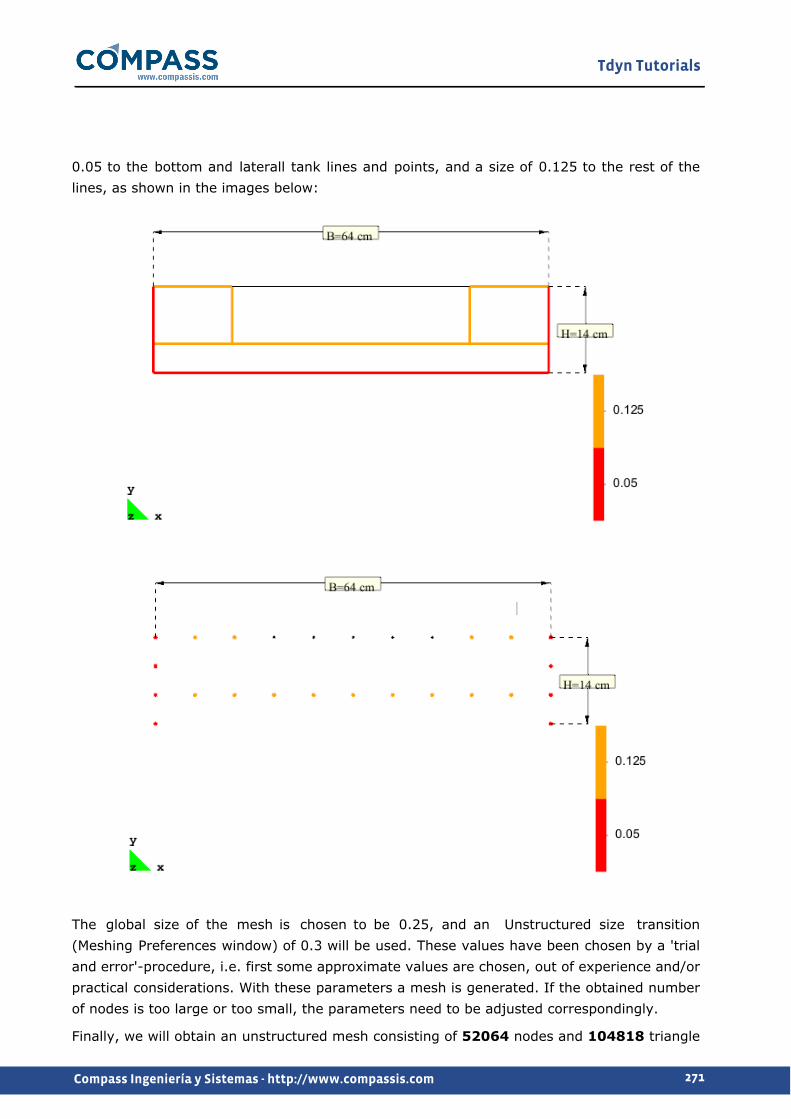
Tdyn Tutorials


0.05 to the bottom and laterall tank lines and points, and a size of 0.125 to the rest of the lines, as shown in the images below:

The global size of the mesh is chosen to be 0.25, and an Unstructured size transition (Meshing Preferences window) of 0.3 will be used. These values have been chosen by a 'trial and error'-procedure, i.e. first some approximate values are chosen, out of experience and/or practical considerations. With these parameters a mesh is generated. If the obtained number of nodes is too large or too small, the parameters need to be adjusted correspondingly.

Finally, we will obtain an unstructured mesh consisting of 52064 nodes and 104818 triangle

Tdyn Tutorials


elements.

Post-processing

Different stages of the simulation are shown below:

t=0.5 s

t=1.0 s

t=1.5 s

Tdyn Tutorials


t=2.0 s

t=2.5 s

Tdyn Tutorials


t=3.0 s

t=3.5 s

t=4 s

Tdyn Tutorials


t=4.5 s

t=5 s

Tdyn Tutorials


2D air quality modeling

Introduction

The following example of this tutorial solves the air pollution transport of a set of two coupled chemical species using a linear air quality model, which accounts for the main physical processes, that is advection, diffusion, coupling between chemical species, wet and dry deposition processes, emission sources and the chemical reactions that take place once the pollutants are emitted. The geometry consists of a two-dimensional space domain, which represents a full air rectangle. The transport of species is produced in this case by the advection in a fluid air and it has been taken into account a unidirectional flow parallel to the x-axis, which has been assumed uniform and constant, given by the vector (0.00045,0.0,0.0) m/s.

Start Data


2D Plane Fluid Species Advection


Pre-processing

The geometry for this tutorial is created using the GID Pre-processor as usually.

First we have to create the point coordinates given below, and then join them into lines (the edges of the control volume).

Tdyn Tutorials


Points:

No: Coordinates:

1. 0.000000 0.000000 0.000000

2. 1.000000 0.000000 0.000000

3. 1.000000 0.250000 0.000000

4. 0.000000 0.250000 0.000000

Then we should create a small line at the left of the space domain representing a stack emission source using for instance the Geometry->Edit->Divide->Lines->Num divisions tool. The number of divisions can be 3. Therefore, the emission source is a line located at the left vertical boundary with a distance equal to 0.083 m.

Finally the external surface of the geometry can be created, by selecting all existing edges. The outcome is the final geometry shown in the introduction section (2D air quality modeling -pag. 276-).

Initial Data

Initial and field data may be specified in the Conds. & Init. Data->Fluid Flow->Initial and FieldData section of the data tree. The values entered in this section will be further used to impose pertinent boundary conditions to the corresponding contours of the model. In this case, the convective wind speed should be fixed to 0.00045 m/s in X-axis and 0.0 in Y-axis to further impose the unidirectional uniform and constant advection velocity over the entire domain.

Species initial data is no longer updated in the Conds. & Init. Data section of the data tree. Instead of that, initial and conditional data are specified individualy for each one of the species in Materials->Edit Species section of the data tree. See Materials -pag. 280- for additional information.

Boundary conditions

Tdyn Tutorials


Fix Concentration

The Conds.& Init Data->Species Advection->Fix Concentration boundary condition can be used to fix the concentration in a particular contour of the model to a given value. This condition must be applied to the left vertical emission source boundary (E) in order to fix there the value of the concentration for each chemical specie. It should be noted here that the value of the concentration should be prescribed separately for each specie at this boundary.

Air pollutants are emitted in the atmosphere from emission sources and suffer chemical reactions, which generate new chemical species. In this way, the air pollutants can be classified into primary pollutants (directly originated from sources) and secondary pollutants (compounds not emitted, formed through the reaction of primary pollutants).

Therefore, in the case of considering two chemical species, then the value of the concentration must be fixed to 1 at the left line of the model geometry representing the emission source (E) with the Specie field set to Specie1 (primary pollutant) and the value of the concentration must be fixed to 0 at the left line of the model geometry (E) with the Specie field set to Specie2 (secondary pollutant). The way to fix the concentration for both chemical species is shown at the figure below. The rest of the space domain will have a zero initial concentration per specie.

Tdyn Tutorials


Advect Flux Fluids

A Robin boundary condition is assigned on the right vertical boundary (A), depending on the direction of the wind speed vector for each chemical specie.

The dry deposition process is represented by the so-called deposition velocity, which is proportional to the absorption at the surface. In fact, the dry deposition is considered in order to include the interaction of both air pollutants with the ground. Therefore, a reactive species flux is assigned on the bottom contour (B), where typical values for dry deposition velocities

Tdyn Tutorials


are used (i.e. vdSpecie1 = -0.0044, vdSpecie2 = -0.0026).

Finally, an impermeability barrier condition or homogeneous Neumann boundary condition is assumed on the top of the space domain (C) and the rest of the left vertical boundary (D-E).

Materials

Fluid

The air material type is assigned to all the surface of the model in order to simulate a full air

Tdyn Tutorials


rectangle at a certain temperature, as shown below.

Species definition

An arbitrary number of species can be defined in the Materials->Edit Species section of the data tree. In this problem we will study two different air pollutants, as shown in the following figure.

The air pollution transport of a set of two coupled chemical species will be automatically solved over the space domain. In this way, a system of two convection-diffusion-reaction

Tdyn Tutorials


equations will be resolved. Notice that the number of equations (two) will be equal to the number of species that should be studied by the model. Fluid properties could be fixed for Specie1 and Specie2 respectively as shown in the following figure. It should be mentioned here that this system is coupled only through the chemical term (f3) and the emission term (f4). The diffusivity coefficient is set to 0.01 in this case.

Problem data

Once the boundary conditions have been assigned and the materials have been defined, additional general information should be introduced in order to solve the problem. The values listed here have to be entered in the Problem, Analysis, Results and pages of the Fluid Dyn. & Multi-phy. Data section of the data tree.

Fluid problem data:

Only SOLVE FLUID ad Solve Species Advection options should be active (the corresponding field value must be equal 1).

Fluid Dyn. & Multi-phy. Data Problem Solve Fluid

All options must be deactivated for solid domains.

Fluid Dyn. & Multi-phy. Data Problem Solve Solid

Tdyn Tutorials


Fluid analysis data:

The following settings should be introduced in


Number of Steps 1200

Time Increment 0.01

Max Iterations 1

Initial Steps 0

Fluid results data:

The following settings should be introduced in


Output Step 25

Result File Binary

Mesh generation

We will generate a 2D mesh by means of GiD's meshing capabilities, selecting the menu option (Ctrl+g)

Mesh Generate mesh

In this example, an unstructured mesh of tetrahedra with a global size of 0.01 m and an Unstructured size transition of 0.6 will be generated. The resulting mesh contains about 2920 nodes and 5838 triangle elements.

Calculate


Tdyn Tutorials


Post-processing

When the analysis is completed and the process has finished, it will be possible to visualise the obtained results by clicking on the Postprocess button. For details on the results visualisation please refer to the Post-processing chapter of the previous examples or to the GiD manual and GiD online help.

The results can be easily visualised using the View Results window, which allows the user to choose the simulation to be represented and the way this will be displayed (see the figure below). In order to visualise the ADVECT results its corresponding Analysis type has to be selected as shown in the following picture.

In what follows we illustrate the results of propagation of both coupled species for successively instants of time. The distribution of concentrations at various time-steps are presented together with their concentrations scale. From its observation we can see the decreasing of the primary pollutant (Specie 1 at left side) due to chemistry and deposition and the generation of the secondary air pollutant (Specie 2 at right side).

Tdyn Tutorials


t = 0.25 s t = 0.25 s

t = 1 s t = 1 s

t = 3 s t = 3 s

Tdyn Tutorials


t = 5 st = 5 s

t = 8 st = 8 s

t = 12 s t = 12 s

6 References

Tdyn Tutorials


1.- E. Oñate and J. García-Espinosa. Finite Element Analysis of Incompressible Flows with Free Surface Waves using a Finite Calculus Formulation. ECCOMAS 2001. Swansea UK 2001.

2.- E. Oñate, and J. García-Espinosa, Advanced Finite Element Methods for Fluid Dynamic Analysis of Ships, MARNET-CFD Workshop, Crete, Athens, 2001.

3.- E. Oñate, and J. García-Espinosa, A Finite Element Method for Fluid-Structure Interaction with Surface Waves Using a Finite Calculus Formulation, Comput. Methods Appl. Mech. Engrg. 191 (2001) 635-660.

4.- E. Oñate and J. García-Espinosa. A methodology for analysis of fluid-structure interaction accounting for free surface waves. European Conference on Computational Mechanics (ECCM99). Munich, Germany, September 1999.

5.- O. Soto, R. Löhner, J. Cebral and R. Codina. A Time Accurate Implicit-Monolithic Finite Element Scheme for Incompressible Flow. ECCOMAS 2001. Swansea UK 2001.

6.- B. F. Armaly, F. Durst, J. C. F. Pereira, B. Schönung, Experimental and theoretical investigation of backward-facing step flow. J. Fluid Mech. 127, 473-496, 1983.

7.- M. A. Cruchaga, A study of the backwards-facing step problem using a generalised streamline formulation. Communications in Numerical Methods in Engineering, 14, 697-708, 1998.

8.- R. Codina, M. Vázquez and O.C. Zienkiewicz, A fractional step method for the solution of the compressible Navier-Stokes equations. Publication CIMNE no. 118, Barcelona 1997.

9.- E. Oñate, J. García-Espinosa y S. Idelsohn. Ship Hydrodynamics. Encyclopedia of Computational Mechanics. Eds. E. Stein, R. De Borst, T.J.R. Hughes. John Wiley and Sons (2004).

10.- J. García-Espinosa and E. Oñate. An Unstructured Finite Element Solver for Ship Hydrodynamics. Jnl. Appl. Mech. Vol. 70: 18-26. (2003).

11.- GiD, A pre/postprocessing environment for generations of data and visualisation in finite element analysis. CIMNE, Barcelona, 1996.

12.- Löhner, R., Yang, E., Oñate, E. and Idelsohn, S. An Unstructured Grid-Based, Parallel Free Surface Solver. Presented in IAAA journal. CIMNE. Barcelona 1996.

Tdyn Tutorials


13.- E. Oñate, J. García and S. Idelsohn, On the stabilisation of numerical solutions of advective-diffusive transport and fluid flow problems. Comp.Meth. Appl. Mech. Engng, 5, 233-267, 1998

14.- J. García-Espinosa, E. Oñate and J. Bloch Helmers. Advances in the Finite Element Formulation for Naval Hydrodynamics Problems. International Conference on Computational Methods in Marine Engineering (Marine 2005). June 2005. Oslo (Norway)

15.- A. Roshko, On the development of turbulent wakes from vortex streets, NACA report 1191, 1954.

16.- M. Vázquez, R. Codina and O.C. Zienkiewicz, A general algorithm for compressible and incompressible flow. Part I: The split characteristic based scheme. Int. J. Num. Meth. in Fluids, 20, 869-85, 1995

17.- M. Vázquez, R. Codina and O.C. Zienkiewicz, A general algorithm for compressible and incompressible flow. Part II: Tests on the explicit form. Int. J. Num. Meth. in Fluids, 20, No. 8-9, 886-913, 1995.

18.- J. García-Espinosa, M. López, E. Oñate, R. Luco, An Advanced Finite Element Method for Fluid Dynamic Analysis of America's Cup Boats, Proceedings of HPYD Conference (RINA), Auckland (New Zealand) 2002.

19.- J. García, A. Valls, E. Oñate. ODDLS:A new unstructured mesh finite element method for the analysis of free surface flow problems. Int. J. Numer. Meth. Engng. Published online, 2008.

Documents

Tdyn Tutorials - Compass · PDF fileTdyn Tutorials Compass Ingeniería ... Taylor-Couette flow 168 Introduction 168 ... The actual value of the Reynolds number is taken to be Re =