TAXES AND PORTFOLIO COMPOSITION Edwin J. ELTON and

Journal of Financial Economics 6 (1978) 399410. 0 North-Holland Publishing Company

TAXES AND PORTFOLIO COMPOSITION

Edwin J. ELTON and Martin J. GRUBER* New York University, New York, NY 10006, USA

Received September 1977, revised version received May 1978

This paper explores investors portfolio behavior when security returns can be described by one of the forms of the CAPM model and investors pay taxes. The conditions under which an investor holds the market portfolio are explored. In addition the extent to which securities are held in proportions which differ from market weights are shown to be functions of tax rates, dividend policies, and the variance covariance structure between all securities.

1. Introduction

The implication that under the Sharpe-Lintner-Mossin form of the CAPM all investors should hold the market portfolio is well known. When one considers the fact that income and capital gains are taxed -at different rates, then except under the special circumstances derived by Long (1977), one will get (1) a different equilibrium relationship for the capital markets (the post- tax CAPM of Brennan), and (2) a different model of optimal investor behavior.

This paper addresses the following problem. Assume an investor recognizing his tax liability wishes to select portfolios on the assumption that either the Sharpe-Lintner-Mossin form or the post-tax form of the CAPM holds. Then what is the optimum portfolio for him to hold? Under what circumstances is it the market portfolio? When it differs from the market portfolio, what are the characteristics of securities that should be held in greater or lesser proportions by any investor?

More precise answers to these questions can be reached if we are willing to make simplifying assumptions about the variancecovariance structure of returns. We shall explore the answers to these problems under two specific models of how covariance structure is determined: the single index model and the constant correlation model. The single index model is standard and needs no introduction here. The constant correlation model is based on the assumption that the correlation coefftcient between each pair of securities can be considered to be constant.’

*The authors would like to thank the Institute for Quantitative Research in Finance for their generous financial support, and the referee, Michael Brennan, for his comments and suggestions.

‘See Elton and Gruber (1973) for an empirical justification of this model,

400 E.J. Elton and M.J. Gruber, Taxes and portfolio composition

2. The general case

In this section of the paper, we examine the optimal portfolio holdings,of investors when no special assumptions are made about the variance- covariance structure of returns. We first assume that investors act as if prices are determined by the capital asset pricing model that results from portfolio decisions being made on the basis of post-tax returns. We then briefly review the results when investors are assumed to act as if the SharpeLintner- Mossin form of the CAPM determines prices. The conclusions we can reach in this section are quite limited and add further motivation for examination of models which assume simplified forms of the covariance structure.

In appendix B we derive the following expression for the portfolio behavior of an investor who is subject to taxes and believes that prices are determined by the post-tax CAPM,

where

Z,,i=HXI,+ (T-Tm)C,, (1)

Z,,i =a number which is proportional to the fraction of the ith investor’s portfolio which should be invested in stock k.

X,= the fraction of the market portfolio which consists of stock k.

H = the market price of risk for the post-tax capital asset pricing model (see appendix A).

T = the difference between the ith investor’s marginal capital gains tax rate and his income tax rate dividend by one minus his capital gains tax rate.

T,= the effective average value of q for the market (see appendix A). C,=a constant for the kth security; CI, is defined in appendix B.

In appendix B of this paper we also derive the optimal portfolio behavior for investors under the assumption of the Sharpe-Lintner-Mossin form of the CAPM. We show that

Zks i = H'X, + l& ,

where H' is the market price of risk for the pre-tax capital asset pricing model.

We will now proceed to examine the implications of eq. (1) for the composition of an investor’s portfolio. If the tax rate for the market is equal to the individual’s tax rate, then the optimal investment for the individual is the market proportions in each security. This conclusion follows from noting that if q= T,, then the second term in eq. (1) is zero. Further, Zki is proportional to the optimal fraction of the ith investors portfolio and

E.J. Elton ond M.J. Cuber, Taxes qnd portfolio composition 401

dividing Z,,i by a constant does not affect this property- of Z,,i. Hence, dividing both sides of eq. (1) by H yields a new Z,,i which is equal to Z;,i. However, the Z;,i are already scaled to add to one so that no further scaling is needed for the new Z; ls.

Consequently, when investors desire to make investment decisions on the assumption that the post-tax capital asset pricing model generates returns in the market place, they hold the market portfolio if the individual’s tax rate equals the market tax rate. Making a parallel argument for eq. (2) if investors wish to make investment decisions based on the assumption that the pre-tax capital asset pricing model reflects risk-return opportunities in the market, then they invest in the market portfolio if the individual’s tax rate is zero.

We can use eqs. (1) and (2) to examine the portfolio composition of investors with different tax rates. In particular, we will examine two questions. First, which securities are held in greater than market proportions and which are held in less. Second, what are the characteristics of a security which determine how ‘unbalanced’ the investor’s portfolio will be with respect to it. For example, if security A and B are held in greater than market proportions which deviates most from its market proportion? To examine the first of these questions, we will compare the percentage of security k in investor i’s portfolio with the percentage security k represents of the market. Let X, represent the market proportion of security k and recognize that Z,:i/x,Z,,i is the fraction of his portfolio that investor i holds in security k. An investor holds more than the market proportion in security k if

Substituting in eq. (1) yields

Hxk+(~-T,)ck>x

k’

H+(T-T,)xCk

k

Rearranging and simplifying shows that security k will be held in greater

than market proportions, if

ck

I

c ck >xk k

<xk

if q>T,, (3)

if K-CT,.


The value of -all terms except Y& are independent of the investor under consideration. All investors with the same relationship of T to T, will hold the same stocks in greater than market proportions. In essence, there are three sets of investors. Investors with T= T, hold market proportions. Investors with T > T, hold stocks with C,/c, Ck >X, in greater than market proportions, stocks with C,/& C, =X, in market proportions and all other stocks in less than market proportions. Finally, the third group of investors for which T< T, act exactly opposite to the second group.

The analysis when the investor wishes to act as if the SharpeLintner- Mossin C.A.P.M. holds is similar. Utilizing eq. (2) in analysis parallel to that just undertaken yields a set of equations identical to eq. (3) except that zero replaces T, in the right-hand set of inequalities. Given the predominance of income tax rates above capital gain tax rates, most investors will tilt their portfolio in favor of stocks with low dividends and it is unlikely that markets will clear at the prices determined by the Sharpe-Lintner-Mossin form of the CAPM.’

The second question worth examining is the condition under which one stock will be held in a higher percentage relative to its market proportions than will a second. Stock j is held in a greater percentage of its market proportion if

zj,i/z zj.i , ‘k,i/F ‘k,i

X; Xk .

Substituting, rearranging and cancelling yields

CjlXj > CJX, if T > T,, (4)

<CL/XL if IT;: < T,. (5)

The value of the C’s and X’s are independent of the investor under consideration. Therefore the relationship of T to T, determines the extent of the deviation of investor f’s portfolio from market proportions. If stock j is held in a greater proportion of its market percentage than stock k for an investor in a tax bracket above the market average tax bracket, then this is true for all investors in tax brackets above the average.

Similar results- hold if the no tax CAPM model adequately describes returns. In this case, the analysis follows from setting T,=O.

We now know that most investors will not hold the market portfolio. To make more precise statements about optimal portfolio composition we must

2Long (1977) presents the necessary and sufftcient conditions for this to happen, and finds empirical evidence is inconsistent with markets clearing at the standard CAPM prices.

E.J. Elton and M.J. Gruber, Taxes and portfolio composition 403

know Ck. But Ck depends on both the excess dividend yield on all stocks and the properties of the inverse of the variance-covariance matrix. More can be learned about investor behavior if we introduce simplifying assumptions about the variance covariance structure of$ecurity returns.

3. The single index model

In this section of the paper we examine the optimal portfolio holdings of investors under the assumption that they estimate the joint movement of securities employing the assumptions of the single index model. Eq. (3) still hblds and the implications of this equation as discussed in section 2 remain valid. However, the special form of the single index model allows us to get more insight into the problem.

In particular, utilizing eq. (B-3) from the appendix, eq. (3) becomes3

Eq. (6) represents the case where general equilibrium is derived in terms of after tax returns. Setting T, =0 would make eq. (6) appropriate for the case where general equilibrium is derived in terms of pre-tax returns (the Sharpe- Lintner-Mossin CAPM).

Note that CO and C, are constants with respect both to all stocks and all investors. Assume for the moment that T < T, or that the investor is subject to a higher tax rate thad the effective tax rate in the market. It is clear from eq. (6) that for positive Beta stocks, the lower the dividend yield, all other things being equal, the more likely the stock is to be held in more than market proportions. Also we see from eq. (6) that if two stocks have identical Betas, residual risk and dividend yields an investor who pays a tax rate higher than the effective average in the market is more likely to hold more than market proportions of the stock which represents a larger share of the market (has a higher X,). An investor with a tax rate lower than the effective rate in the market will act in the opposite manner.4

If we employ the pre-tax equilibrium model, all of the above analysis holds except that zero should be substituted for T,. That is, the investors’ reaction to dividend yield is determined by whether his tax rate on ordinary income is

‘This inequality assumes that C, is positive. C, can be negative, in which case the inequality in each of these equations is reversed. However, since C, is negative with the inequality reversed, all of the discussion which follows still holds.

4Whether an investor invests in more than market proportions in high Beta stocks depends on the sign of Co. If C,<O (a likely case) investors in high tax brackets will favor low Beta stocks-ceteris paribus.

D

404 E.J. Elton ond M.J. Gruber, Taxes and portfolio composition

greater than or less than his tax on capital gains, rather than average tax rate in the market.

the effective

We can learn about the characteristics of stocks in which an investor unbalances the most by substituting eq. (B-3) in eqs. (4) and (5). For an investor with a tax rate above the average rate in the market, we find that for stock j to be held in a larger proportion relative to its market weight than stock k is held relative to its market weight,

It is clear from the above expression that for positive Beta stocks, the lower the dividend yield on a stock the more likely (other things being equal) it is to be held in a higher percentage of its market proportion. If an investor is subject to a tax rate which is lower than the effective average rate in the market, the above inequality is reversed and the investor is likely to unbalance in favor of high dividend paying stocks.’

4. The constant correlation model

This section of the paper will parallel the previous section but will make an alternative assumption about the mechanism generating the covariance structure of security returns. Specifically, we will assume that the correlation coefficient between the returns on all pairs of stocks is the same.

Employing eq. (B-4), eq. (3) can be written as6

<X, for q<Tm.

A similar set of expressions follow with respect to the pre-tax CAPM model. The difference is that T, is replaced with zero in the inequalities on the right side of eq. (7). Once again, as in section 3, we see that the investor who pays a higher tax than the average for the market is more likely to hold stocks with low dividend yields in more than market proportions. Furthermore, for two stocks with the same characteristics, he is more likely to hold the one which represents a large share of the market in more than

50nce again, if the pre-tax CAPM is assumed to hold the above analysis follows except that the effect of dividend yield is found by comparing the investor’s differential tax rate with a rate of zero, rather than the average effective rate in the market.

6The mathematical expressions for Ca and C1 are different from those in the last section of the paper. They follow directly from eqs. (3-4) and (3).

E.J. Elton and M. J. Gruber, Taxes and portfolio composition 405

market proportions.’ Investors who pay taxes at a rate below the market average will act in the opposite manner.

We can learn more about which of two stocks will be held in larger proportions relative to their market proportions by making use of the special properties of the constant correlation model. In particular, eq. (3) can be written as

Cr<C;$ where Cj*=C,(l-p). k

Making use of eq. (B-4) the CT’s can be interpreted as a very good approximation of the amount by which a stock’s dividend yield minus the risk-free rate divided by the stock’s standard deviation exceeds the average of the same ratio for the market, with the difference divided by the stock’s standard deviation.* This inequality then says that an investor who has a tax rate higher than the average tax rate in the market will hold less of a stock (relative to its share in the market) as compared with a second stock if the first stock has a higher C* relative to its market share than does the second. Thus, the investor with the higher than average tax rate will not hold the market portfolio but will tilt his portfolio in favor of stocks with lower dividends and lower standard deviations.

The analysis for an investor with a tax rate lower than the effective average tax rate in the market is directly analogous and this investor should behave in the opposite manner from the case discussed above.

There is one more case than can further clarify the implications of this analysis for optimum investor behavior. Let us identify the stock k such that C: =O. This stock k is a stock which has a (6, - RF)/ok (excess dividend yield to risk) approximately equal to the average excess dividend yield to risk of all stocks in the market.’ If Cjj‘ = 0, eq. (9) becomes CT < 0 for investors with tax rates above the average effective tax rate in the market. Thus investors

‘For the case where investors make decisions based on pre-tax equilibrium, the analysis holds with the market average tax rate replaced by a zero tax rate.

*To be more exact,

P w &-RF c- l-p+Np,=, 0, l 1 0’~ + (1 -p))((aj-R~)/uj)-NpAVG((Gt -RF)/~~) =- uj NP+u-P) 9To be more exact,

1 .

4-b NP 4-4 4-R, -= Np+U-PI

AVG - zAVG----. Uk gt 0,


with tax rates above the effective average should all place a higher fraction of their funds (relative to market proportions) in stocks which have a ratio of excess dividend yields to standard deviation below the average than they place in the stock which has an excess dividend yield to standard deviation equal to the average. Since the inequality is reversed for investors with tax rates below the average, they will hold more of their portfolio in high dividend paying stocks and less in low dividend paying stocks. Once again, in the case where the standard CAPM is believed to hold, the above analysis follows if zero is substituted for the average market tax rate.

5. Conclusion

In this paper, we have investigated the impact of personal taxes on the optimum portfolio composition of individual investors. We have demonstrated that even if the investor believes that the standard form of the CAPM is an exact description of returns in the market, he might not hold a market portfolio if he must pay taxes. We have investigated the properties of these stocks that he will hold in more than market proportions and those that he will hold in less than market proportions. The results indicate that if investors look at post-tax returns the market is unlikely to clear at prices set by the standard CAPM model. We have then derived a post-tax CAPM model and demonstrated the optimum portfolio holdings for investors if this model describes returns in the market. Under the post-tax capital asset pricing model as under the standard CAPM, the optimal portfolio holdings of investors becomes a function of the investor’s tax rate, the dividend yield on alternative securities, and the risk characteristics of alternate securities. Pettit and Stanley (1977) use survey data on individual investor portfolio composition to analyze whether taxes influence portfolio choice. Consistent with the predictions of this analysis, they find that there is a significant relationship between investor tax rates and portfolio choice.

Appendix A

In this appendix we derive a Capital Asset Pricing Model assuming investors make portfolio decisions on the basis of post-tax returns. An alternative proof of the post-tax capital asset pricing is contained in Brennan (1970). We shall make the normal assumption of homogeneous beliefs about pre-tax returns. However, since different investors are subject to different tax rates, beliefs about the post-tax returns will be different.

As shown in Lintner (1965) the portfolio problem can be viewed as maximizing the ratio of excess returns to risk. lo Expressing this in after-tax

“Lintner’s equations are presented in terms of return. Since we are assuming investors are concerned with post-tax returns, the equations hold with respect to post-tax returns for each investor.


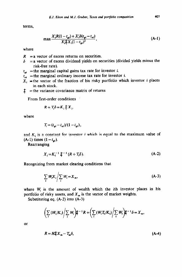
terms,

max XIR( 1 - t,*) + x;s(t,, - toi)

X$Xi( 1 - Cgi)2 ’ (A-1)

where

R =a vector of excess returns on securities. 6 = a vector of excess dividend. yields on securities (divided yields minus the

risk-free rate). tgi = the marginal capital gains tax rate for investor i. tOi = the marginal ordinary income tax rate for investor i. Xi = the vector of the fraction of his risky portfolio which investor i places

in each stock. $ = the variance covariance matrix of returns

From first-order conditions

R+ ~~=KiIXi,

where

and Ki is a constant for investor i which is equal to the maximum value of (A-l) times (1 - tJ.

Rearranging

Xi=K;’ I-'(R+11;-6). (A-2)

Recognizing from market clearing conditions that

(A-3)

where K is the amount of wealth which the ith investor places in his portfolio of risky assets, and X, is the vector of market weights.

Substituting eq. (A-2) into (A-3)

or

R = H$X, - T,6, (A-4)


where

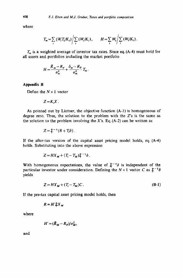
lY=Cw C(B$/Ki)s

i Ii

T, is a weighted average of investor tax rates. Since eq. (A-4) must hold for all assets and portfolios including the market portfolio

Appendix B

Define the N x 1 vector

Z=KJ.

As pointed out by Lintner, the objective function (A-l) is homogeneous of degree zero. Thus, the solution to the problem with the Z’s is the same as the solution to the problem involving the X’s. Eq. (A-2) can be written as

Z=$-‘(R+T6).

If the after-tax version of the capital asset pricing model holds, eq. (A-4) holds. Substituting into the above expression

With homogeneous expectations, the value of $-‘S is independent of the particular investor under consideration. Defining the N x 1 vector C as $- ‘6 yields

Z=HX,+(T-T,)C. (B-1)

If the pre-tax capital asset pricing model holds, then

where

H' = (RM - RF)/&

and


Z=H’X,+~C. (B-2)

If one is willing to make special assumptions about the variance-covariance matrix then simplified forms of the inverse of the variancecovariance matrix exist and C has some interesting special forms. Two assumptions about the variance4ovariance matrix are known to yield simple structures for the inverse of the variance-covariance matrix; these are the variance-covariance matrix that result from assuming the single index model and the variance- covariance matrix that results from assuming the correlation coefficient is a constant between any pair of securities. If the single index model is assumed, the main diagonal element of the inverse of the variancecovariance matrix in row k has a value equal to

l+ uif c .$,

( -------1

uZ,k l +a& i (P,“l”f, j)

j=l 1 where O& is the variance of the residuals from the single index model for the kth stock. The off-diagonal element k,j for j> k is equal to

The off-diagonal element k, j for k > j is

- &J:b:k)

u:k 1+ 4 5 ( u-$/4,,) p=l )’

Using these expressions to determine C yields for the kth row

c =&

i

6k-b TL jcl {(~j-R,)Bj/~f,ji)

O8.k l+Oif ; (8fl"f,j)

j=l

k 2 ___-

811 (B-3)

This expression was derived in another context in Elton, Gruber and Padberg (1976).

If one assumes that the correlation coefficient between any two securities is the same and is equal to p, then the element jj of the inverse of the


variance-covariance matrix is equal to

(1 + PW4 Cl-P)(l+W-lIPI’

the off-diagonal elements in row k, column j are equal to

Using these expressions to determine C yields for thejth row

P N Sk-RF

I-p+Np,,,ol, ’ c 1 (B-4)

Once again, this was derived in another context by Elton, Gruber and Padberg (1976).

References

Brennan, Michael, 1970. Taxes, market valuation and corporate financial policy, National Tax Journal, 417-427.

Elton, Edwin J., Martin J. Gruber and Manfred Padberg. 1976, Simple criteria for optimal portfolio selection, Journal of Finance, 1341-1348.

Elton, Edwin J. and Martin J. Gruber, 1973, Estimating the dependence structure of share price- Implications for portfolio selection, Journal of Finance, 1203-1232.

Lintner, John, 1965, The valuation of risky assets and the selection of risky investments in stock portfolios and capital budgets, Review of Economics and Statistics 47, 13-37.

Long, John, 1977, Efficient portfolio choice with dilIerential taxation of dividends and capital gains, Journal of Financial Economics 5, no. 1, 25-54.

Pettit, Richard, 1977, Consumption-investment decisions with transactions costs and taxes: A study of the clientel e&ct of dividends, Journal of Financial Economics 5, no. 3.

Documents

TAXES AND PORTFOLIO COMPOSITION Edwin J. ELTON and