Tax-versus-trading and efficient revenue recyclingas issues for greenhouse gas abatement

Final authors’ manuscript, now published as

Journal of Environmental Economics and Management, 64, 230-236 (2012)

John C.V. Pezzeya,b,*, Frank Jotzoc

aFenner School of Environment and Society, Australian National University,

Canberra, ACT 0200, AustraliabVisiting Fellow, Department of Economics, University of Bath, BA2 7AY, UKcCrawford School of Public Policy, Australian National University, Canberra, ACT

0200, Australia

*Corresponding author at: Fenner School, Building 141, Australian National University, Canberra,

ACT 0200, Australia

Email address: jack.pezzey@anu.edu.au (J.C.V. Pezzey)

URL: http://people.anu.edu.au/jack.pezzey (J.C.V. Pezzey)

Keywords: emission pricing, tax-versus-trading, uncertainties, revenuerecycling, climate policy, global

Abstract. We give empirical welfare results for global greenhouse gas

emission abatement, using the first multi-party model to include both

tax-versus-trading under uncertainties, and revenue recycling. Including

multiple, independent parties greatly reduces the welfare advantage of an

emissions tax over emissions (permit) trading in handling abatement-cost

uncertainties, from that shown by existing, single-party literature. But a

previously ignored and much bigger advantage of a tax, from better handling

uncertainties in business-as-usual emissions, greatly boosts the overall tax-

versus-trading advantage. Yet the degree to which each mechanism is used to

raise and recycle revenue efficiently by lowering distortionary taxes − rather

than recycle revenue as lump sums, or not raise revenue by giving tax

thresholds or free permits − may in turn dominate any tax-versus-trading

advantage. Choosing the best greenhouse abatement mechanism should thus

consider the issues of tax-versus-trading and efficient revenue recycling

together.

1. Introduction

Designing policy mechanisms for abating greenhouse gas emissions

cost-effectively grows ever more important, as scientists recommend ever

stronger abatement to avoid dangerous climate change [1]. For decades

economists have promoted emission pricing − market mechanisms

(economic instruments) like a carbon (emissions) tax or (carbon) emissions

(permit) trading − for such abatement. Compared to directly regulating

millions of greenhouse emitters, pricing can minimise total abatement costs

by equalising emitters’ otherwise very diverse marginal abatement costs.

It can also avoid huge administration costs.

Also for decades, economists have debated which emission pricing

mechanism is most cost-effective, especially the choice between direct

"prices" (a tax) and indirect prices via "quantities" (tradable permits) under

abatement-cost uncertainty, following Weitzman’s [20] seminal, partial-

equilibrium analysis. However, uncertainties other than in abatement costs

also affect this choice, and we will show that uncertainties in each party’s

(country’s or region’s) future, business-as-usual (BAU) emissions are even

more important. And since the early 1990s, another key issue in the

mechanism-choice debate applied to greenhouse abatement has been the

welfare-reducing, general-equilibrium interaction between emission pricing

and existing, conventional taxes on other factors of production (labour

and/or capital). This shows the importance of both raising revenue from

emission pricing, and then recycling it to raise welfare − usually assumed

to be done by cutting rates of factor taxation and thus the distortionary

welfare losses of such taxation [3,4], even though this rarely happens in

practice.

2

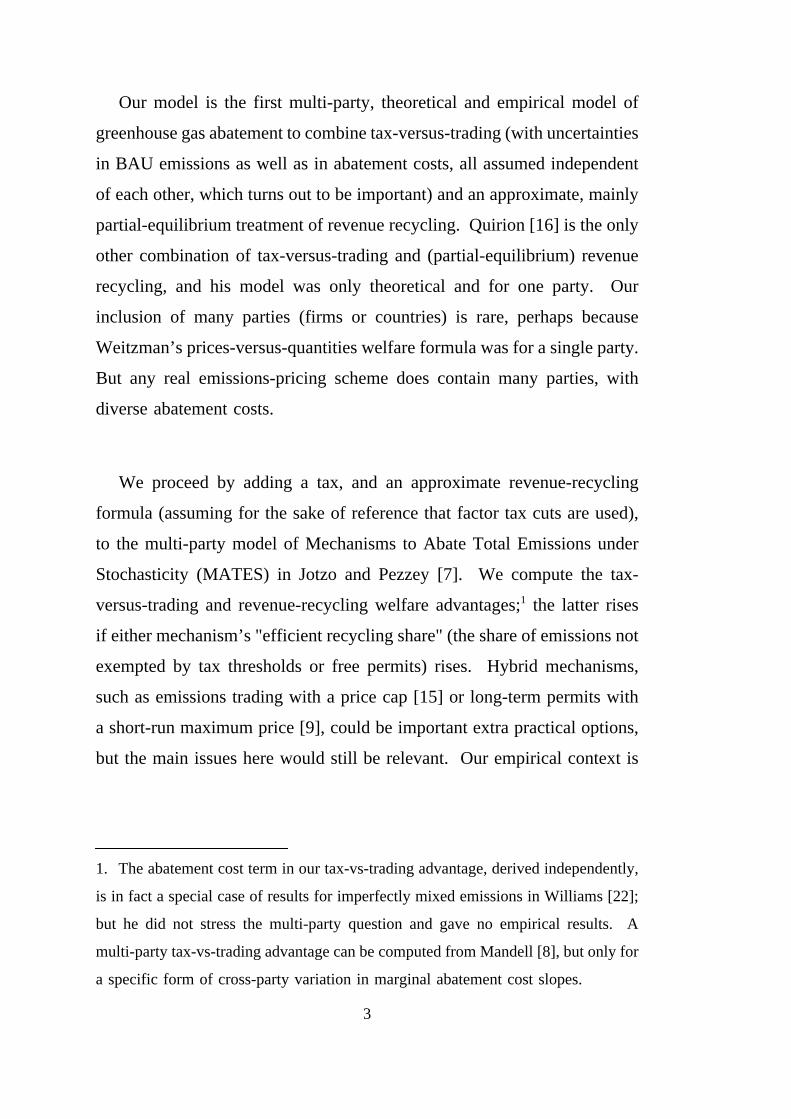
Our model is the first multi-party, theoretical and empirical model of

greenhouse gas abatement to combine tax-versus-trading (with uncertainties

in BAU emissions as well as in abatement costs, all assumed independent

of each other, which turns out to be important) and an approximate, mainly

partial-equilibrium treatment of revenue recycling. Quirion [16] is the only

other combination of tax-versus-trading and (partial-equilibrium) revenue

recycling, and his model was only theoretical and for one party. Our

inclusion of many parties (firms or countries) is rare, perhaps because

Weitzman’s prices-versus-quantities welfare formula was for a single party.

But any real emissions-pricing scheme does contain many parties, with

diverse abatement costs.

We proceed by adding a tax, and an approximate revenue-recycling

formula (assuming for the sake of reference that factor tax cuts are used),

to the multi-party model of Mechanisms to Abate Total Emissions under

Stochasticity (MATES) in Jotzo and Pezzey [7]. We compute the tax-

versus-trading and revenue-recycling welfare advantages;1 the latter rises

if either mechanism’s "efficient recycling share" (the share of emissions not

exempted by tax thresholds or free permits) rises. Hybrid mechanisms,

such as emissions trading with a price cap [15] or long-term permits with

a short-run maximum price [9], could be important extra practical options,

but the main issues here would still be relevant. Our empirical context is

1. The abatement cost term in our tax-vs-trading advantage, derived independently,

is in fact a special case of results for imperfectly mixed emissions in Williams [22];

but he did not stress the multi-party question and gave no empirical results. A

multi-party tax-vs-trading advantage can be computed from Mandell [8], but only for

a specific form of cross-party variation in marginal abatement cost slopes.

3

an 18-region world in 2020, representing a short run when the global

greenhouse gas stock is very large compared to emissions flow.

2. A model with tax-versus-trading and efficient revenue recycling

2.1 The theoretical model

Emissions are perfectly mixed in a common environment used by n

unevenly sized parties (firms, countries, or regions of countries) indexed by

i = 1,...,n, so our theoretical results apply generally to well-mixed

pollutants. An absent subscript i means summation (Z := ΣiZi for any {Zi});

while a tilde,~, means an uncertain (stochastic) variable, and its absence

denotes an expectation (Zi := E[Z~

i]). Each party’s uncertain, BAU emission

in say tonnes/year (t/yr) at a single future date is2:

E~b

i = Ebi (1+εEi), where3

εEi = proportional uncertainty in i’s emission, with E[εEi2] =: σEi

2, (1)

and importantly, all errors are assumed independent with zero means4:

E[εEiεEk] = 0 ∀i≠k, and E[εEi] = 0. (2)

2. In estimating E[εEi2] empirically, Jotzo and Pezzey (p263) combined uncertainties

in GDP, in emissions intensities of GDP, and in non-GDP-linked emissions.

3. Note the distinction between E[.] for the expectation operator, and Ebi , Eb, etc for

various measures of BAU emissions.

4. The effect of positive cross-party emission correlations is separately addressed

in Section 2.2.

4

Each party abates its emissions by an uncertain Q~

i t/yr in response to a

tax or trading mechanism created by an "authority" (a global treaty or a

national law, with full participation and enforcement assumed). We will

compare the market-wide (i.e. social) net benefits for each mechanism of

achieving a given target X for expected total emissions:

X = E[Σi(E~b

i−Q~

i)] = Eb−Q, (3)

given that each party’s uncertain abatement cost is C~

i(Q~

i) in say $/yr.5

With an emissions tax, denoted P for Price, the authority chooses a

certain tax rate pP (in $/t) so that Q, the expected sum of abatements Q~

i(pP)

− which each party chooses to equate its marginal abatement cost (MAC)

C~

i′(Q~

i) with pP − equals the expected abatement task, Eb−X (assumed

positive). The authority also levies only some share ρ of the potential,

expected tax revenue pPX, by giving each party i a tax threshold (1−ρ)Xi

(0 ≤ ρ ≤ 1, Xi > 0) as a quasi-property right.6 This preserves long-run,

partial−equilibrium efficiency by making pP apply to emitters’ exit-entry

decisions, but does not affect Q. Under certainty a threshold (1−ρ)Xi is

symmetric with giving (1−ρ)Xi free tradable permits (Pezzey [12], who

called the tax threshold a "baseline for a charge-subsidy"). It is thus an

inframarginal tax exemption for i, as distinct from exempting i completely

from the tax, here called an exclusion. Exclusions and dilutions (lower

5. We thank a referee for noting that welfare maximisation for a tax and for trading

do not necessarily result in the same expected abatement Q, unless marginal

abatement costs and benefits are linear, as in fact we assume below.

6. The only constraint on the {Xi} here is ΣiXi = X, so assuming the same ρ for all

parties still allows the authority to choose the distribution {(1−ρ)Xi} on political

grounds.

5

rates for selected emitters) are frequent practical occurrences (see for

example Svendsen et al. [19]), but they remain outside our model.

With emissions trading, denoted T, the authority creates X tradable

permits (again < Eb), auctions ρX permits, and gives each party (1−ρ)Xi

free permits.7 Permit trading then establishes an uncertain permit price

p~T (unaffected by ρ), and each party chooses abatement Q

~i(p

~T) to equate

its MAC C~

i′(Q~

i) to this price. Permit-market clearing ensures that total

abatement Q~(p~T) equals the required abatement E

~b−X.

Denoting either tax rate pP or permit price p~T in our model by emission

price p~, with either tax or trading, the authority thus gets revenue R

~i :=

p~[E

~bi−Q

~i(p

~)−(1−ρ)Xi] from party i. This will be negative for any party i

whose abated emissions fall below its threshold or free permit level

(E~b

i−Q~

i(p~) < (1−ρ)Xi); but we assume ρ is chosen high enough to make

total revenue R~

positive.

We call ρ the mechanism’s efficient recycling share, but this term needs

careful explanation. ρ is the share of potential revenue p~X which is both

raised (rather than not raised in the first place by giving tax thresholds or

free permits) and recycled efficiently (as lower rates of existing factor

taxation, thus lowering the welfare cost of existing, distortionary taxation,

rather than as lump sums). Efficient recycling is assumed by almost all

tax-interaction literature, even though it has rarely happened in practice.8

7. Jotzo and Pezzey’s uncertain targets {X~

i} included intensity (indexed) targets, but

this extension would distract from our focus here.

8. A notable exception is the Australian carbon pricing legislation due to come into

effect in mid-2012 [2]. This will recycle about half of the permit revenue to

households, mainly as reductions in income taxes.

6

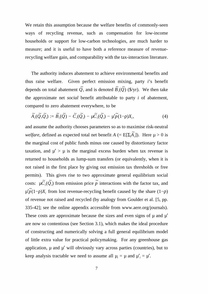
We retain this assumption because the welfare benefits of commonly-seen

ways of recycling revenue, such as compensation for low-income

households or support for low-carbon technologies, are much harder to

measure; and it is useful to have both a reference measure of revenue-

recycling welfare gain, and comparability with the tax-interaction literature.

The authority induces abatement to achieve environmental benefits and

thus raise welfare. Given perfect emission mixing, party i’s benefit

depends on total abatement Q~, and is denoted B

~i(Q

~) ($/yr). We then take

the approximate net social benefit attributable to party i of abatement,

compared to zero abatement everywhere, to be

A~

i(Q~,Q

~i) := B

~i(Q

~) − C

~i(Q

~i) − µC

~i(Q

~i) − µ′p~(1−ρ)Xi , (4)

and assume the authority chooses parameters so as to maximise risk-neutral

welfare, defined as expected total net benefit A (= E[ΣiA~

i]). Here µ > 0 is

the marginal cost of public funds minus one caused by distortionary factor

taxation, and µ′ > µ is the marginal excess burden when tax revenue is

returned to households as lump-sum transfers (or equivalently, when it is

not raised in the first place by giving out emission tax thresholds or free

permits). This gives rise to two approximate general equilibrium social

costs: µC~

i(Q~

i) from emission price p~

interactions with the factor tax, and

µ′p~(1−ρ)Xi from lost revenue-recycling benefit caused by the share (1−ρ)

of revenue not raised and recycled (by analogy from Goulder et al. [5, pp.

335-42]; see the online appendix accessible from www.aere.org/journals).

These costs are approximate because the sizes and even signs of µ and µ′

are now so contentious (see Section 3.1), which makes the ideal procedure

of constructing and numerically solving a full general equilibrium model

of little extra value for practical policymaking. For any greenhouse gas

application, µ and µ′ will obviously vary across parties (countries), but to

keep analysis tractable we need to assume all µi = µ and µ′i = µ′.

7

Finally, we assume quadratic cost and benefit functions:

C~

i(Q~

i) := ½(1/Mi)Q~

i2 + εCiQ

~i, where (5)9

{Mi} > 0 are parameters, and 1/M is the total MAC curve’s slope;

εCi is i’s uncertainty in MAC, with

E[εCi] = 0 and E[εCi2] = σCi

2 for all i, and each εCi is assumed

independent of all other uncertainties in the model. (6)10

B~

i(Q~) := ViQ

~− ½WiQ

~2, where Vi > 0, Wi > 0. (7)

We call V the linear valuation of abatement, while W is the slope of

the total marginal abatement benefit (MAB) curve.11

The net social benefit (4) attributable to party i is thus

A~

i = ViQ~

− ½WiQ~2 − (1+µ)[½(1/Mi)Q

~i2 + εCiQ

~i] − µ′(1−ρ)Xip

~. (8)

We can then show (see online material) that the optimal welfare from

an emissions tax mechanism is

AP = A* + ½Σi[(1+µ)/Mi − W ]Mi2σCi

2, (9)

9. A referee noted that this additive form of uncertainty, used by Weitzman (eq.

(10)) and many authors since, makes C~

i′(0) = εCi, so MAC could be negative at zero

abatement. This awkward possibility would be avoided by assuming multiplicative

uncertainty, as in Hoel and Karp [6]. We still use (5), both to make our results

comparable to the Weitzman-inspired literature, and because we consider only large-

abatement situations where MAC < 0 is very unlikely.

10. The independence assumption is crucial for our results and is discussed below.

11. We ignore any shift stochasticity in i’s MAB, which does not affect the tax-

versus-trading comparison. We thus also ignore any correlations between MAB and

MAC uncertainties, which do affect the comparison (Stavins 1996). For nations’

emissions of greenhouse gases, there is no evidence for such correlation.

8

and from an emissions trading mechanism is

AT = A* + ½Σi[(1+µ)/Mi − (1+µ)/M]Mi2σCi

2

− ½[(1+µ)/M+W]Σi(Ebi)

2σEi2, (10)

where welfare under certainty from either mechanism is

A* := ½[V − (1−ρ)µ′Eb/M]2M / [1+µ+WM−2(1−ρ)µ′]. (11)

Hence the tax-versus-trading (welfare) advantage is

∆ := AP−AT = ½[(1+µ)/M − W]ΣiMi2σCi

2 + ½[(1+µ)/M+W]Σi(Ebi)

2σEi2; (12)

while the optimal, expected emission price and total abatement are

p* = [V−(1−ρ)µ′Eb/M] / [1+µ+WM−2(1−ρ)µ′], Q* = Mp*. (13)

For use later, we also write the trading welfare including only abatement-

cost uncertainties ((10) minus the last term) as

ATC := A* + ½Σi[(1+µ)/Mi − (1+µ)/M]Mi

2σCi2. (14)

An implicit assumption here is that price p* > 0, hence the efficient

recycling share ρ > 1−(VM/µ′Eb) when µ′ > 0; otherwise marginal

abatement actually lowers welfare, as stressed by Goulder et al. [5]. For

values of ρ and µ′ plausible in our greenhouse application, this is a

feasible, though far from non-trivial condition, as will be seen.

2.2 Features and qualifications of the total expected welfare results

Three features of the above results deserve comment. The first, novel

and empirically most important economic result is that in (12), BAU

emissions uncertainties add ½[(1+µ)/M +W] Σi(Ebi)

2σEi2 to the tax-versus-

trading advantage. Intuitively, this arises from emissions uncertainties

being a second source of emission price uncertainty under trading, and thus

9

a second advantage of the fixed price under a tax. It deserves a good deal

more attention, because in our global, greenhouse case study, it easily

dominates the first, abatement-cost term in (12).

Next, note that in our model the efficient recycling share ρ affects only

the certainty welfare A*, not the advantage ∆. So in principle the choice

of efficient recycling share is separate from the tax-versus-trading choice.

In practice, though, we think current institutional and political realities

mean the two choices are tightly connected and for that reason alone need

to be considered together, as opined in our Conclusions.

A third, more complex feature, though empirically less important for our

greenhouse case, is the effect of including multiple, independent parties on

the first, abatement cost term in the advantage (12), which we write as

∆C := ½[(1+µ)/M −W]ΣiMi2σCi

2. (15)12

This is indeed an advantage (∆C > 0) for short-run greenhouse emissions,

because the large existing pollutant stock means the total MAB curve is

relatively very flat (W << (1+µ)/M) [15]. But if a single representative

party, denoted 1, is assumed, (15) becomes

∆C1 := ½[(1+µ)/M −W]M2σC2. (16)

After converting notation and setting µ = 0, ∆C1 is the main result given by

Weitzman’s [20] result (20).13 The ratio ∆C1/∆C depends on the

distribution of party sizes, but is probably much larger than one, and is

12. With converted notation, µ = 0 and changed sign, this is Williams’ [22] result

(34) for "when the goods are perfect substitutes", as in globally well-mixed pollution.

13. Though Weitzman’s footnote 1 on p490 clearly envisaged an application to

emissions trading, he did not give any multi-party trading formula. His Section V

computed the many-party advantage of prices over non-traded quantities.

10

about 9 in our empirical model. So the single-party formula ∆C1, which

ignores how trading dampens the transmission of many parties’

(independent) cost uncertainties into uncertainty in the permit price,

significantly overestimates the advantage of a tax over realistic permit

trading (or of trading over tax, in a different empirical case with W >

(1+µ)/M). This could matter, because the well-known, climate-related

literature on prices-versus-quantities uses the single-party formula ∆C1 (with

µ = 0): see for example Hoel and Karp [6], Pizer [15] and Newell and

Pizer [10]. We could not find any empirical study of tax-versus-trading for

greenhouse emissions abatement which both uses Weitzman’s theoretical

foundation and allows for multi-party trading.

However, the tax-versus-trading advantage is partly restored in the

greenhouse case by two considerations about correlations, which remain

off-model in the absence of suitable data.14 First, while some

determinants of abatement costs like fuel mix vary greatly across countries,

other determinants like energy-saving technologies and before-tax fuel

prices are now fairly globalised. So in practice there will be some positive,

cross-party correlation in cost uncertainties [17], and our independence

assumption in (6) is overstated. Indeed, under the opposite, also overstated,

assumption of identical, perfectly correlated {εCi}, ∆C reverts to the single-

party form ∆C1 (see online material). Second, if emissions uncertainties are

correlated rather than independent across parties, so that E[εEiεEk] =: σEik ≠

0 for several i ≠ k, then Σi(Ebi)

2σEi2 in (10) and (12) is replaced by

Σi(Ebi)

2σEi2 + 2Σi≠kE

biE

bkσEik (see online material). Assuming positive

correlations outweigh negative ones (Σi≠kEbiE

bkσEik > 0), as seems reasonable

for example in the 2008 global recession, this also increases the tax-versus-

trading advantage.

14. We thank the referees for both these points.

11

3. Empirical results for climate policy

3.1 Parameters chosen

Our application of MATES is to static abatement of greenhouse

emissions in 2020, in a world with 18 regions that differ greatly in GDP

and other parameters. The parameters used to calculate results (9)-(16) for

optimal, global welfare are in Table 1; their empirical calibration is

explained in Jotzo and Pezzey [7].

Table 1 Key global parameters in 2020 in MATES($ = US$ in 2000; t = tonne of CO2-equivalent)

Parameter Notation and value

BAU greenhouse gas emissions Eb = 54.4 Gt/yr (= 1.3E2002)

Linear valuation of abatement V = 21.9 $/t

MAC slope 1/M = 2.32 ($/t)/(Gt/yr)

MAB slope W = 0.22 ($/t)/(Gt/yr)

Uncertainties in abatement costsΣiMiσCi

2 = 7.60 G$/yr

ΣiMi2σCi

2 = 0.37 (Gt/yr)2

Uncertainties in BAU emissions Σi(Ebi)

2σEi2 = 11.35 (Gt/yr)2

The remaining numbers used in our model are ρ, the efficient recycling

share; µ, the marginal cost of public funds minus one; and µ′, the marginal

excess burden. The efficient recycling share ρ is chosen by national

governments under strong political constraints. Most economists assume

µ′ > 0, hence a potential revenue-recycling efficiency gain, and thus

recommend full revenue raising and recycling (ρ = 1) on welfare grounds.

But with emissions trading, governments typically have found it difficult

to resist industry lobbying to give away many tradable permits for free, at

12

least initially. So as useful values to consider, without prejudging which

may be most realistic, we choose

ρ = 1 or 0.5 for all regions. (17)

For our main results we choose the benchmark values from Goulder et

al. [5, p335 and p342],

µ = 0.1 and µ′ = 0.3. (18)

However, estimates of µ and µ′ are now very contentious. By including the

status (relative consumption) externalities, Wendner and Goulder [21]

estimated a range of µ′ from −0.27 to 0.91, depending on other parameters

chosen, significantly lower than previous authors’ estimates. So in the next

section we also discuss the case µ′ = 0, which greatly changes one of our

results.

3.2 Results

Table 2 shows results, from inserting values from Table 1 and (17)-(18)

into (9)-(16), in four sections. The first gives total welfare from a tax (AP

in (9)) and from trading (AT in (10)), and trading welfare with abatement-

cost uncertainties only (ATC in (14)). The second shows that our complete,

multi-party, tax-versus-trading advantage (∆ in (12)) greatly exceeds the

advantage with only abatement-cost uncertainties counted (∆C in (15)). (No

different ρ or V values are shown, since neither parameter affects the ∆

formulae.) This reflects how emissions uncertainties dominate the ΣiMi2σCi

2

term for abatement-cost uncertainties in Table 1. As discussed in Section

2.2 and shown here, this dominance would be weakened only slightly if

one assumed perfect correlation in abatement cost uncertainties and thus

13

replaced ∆C with the single-party result ∆C1, about 9 times larger than ∆C.

As also discussed there, dominance would be strengthened by likely

correlations in emissions uncertainties.

Table 2 MATES results for global greenhouse abatement in 2020

Marginal cost of public funds − 1

Marginal excess burden

µ = 0.1

µ′ = 0.3

Efficient recycling share of global target, ρ(= 1 − tax thresholds’ or free permits’ share)

1 ("pure"

mechanism)

0.5

Welfare in 2020 (expected global net benefit in US2000 G$/yr) from:

optimal emissions tax with thresholds (AP ) 90.6 6.3

optimal emissions trading with abatement-cost

and emissions uncertainties (AT )

74.4 −9.9

optimal emissions trading with abatement-cost

uncertainties only (ATC )

90.2 5.8

Optimal tax-versus-trading welfare advantage (independent of ρ or V) from:

abatement cost and emissions uncertainties,

multi-party (∆ = AP−AT )

16.2

abatement-cost uncertainties only,

multi-party (∆C = AP−ATC )

0.4

abatement-cost uncertainties only, single-party (∆C1) 3.8

Welfare lost from only 0.5 efficient recycling share (A*(ρ=0.5) − A*(ρ=1)),

for either optimal mechanism:

− with standard linear valuation V −84.3

− with doubled linear valuation −196.9

Other expected results for either optimal mechanism:

emission price p* ($/tCO2-equivalent) 18.3 3.3

abated emissions Eb−Q*, c.f. BAU emissions in 2020 −15% −3%

14

Yet Table 2’s third section highlights a striking feature in the first

section, that the full tax-versus-trading advantage of 16.2 G$/yr is in turn

dominated by the welfare loss of 84.3 G$/yr caused by lowering the

efficient revenue-recycling share ρ from 1 to 0.5. This loss means

emission pricing has negligible or even negative welfare when ρ = 0.5; and

the loss more than doubles again under the sensitivity test of doubling the

linear valuation V. However, all this crucially depends on the benchmark

value of µ′ = 0.3. If the marginal excess burden instead happens to be µ′

= 0 for status reasons discussed after (18), then from (11), varying ρ, the

extent of revenue raising and recycling, has absolutely no effect on welfare.

Lastly, the higher expected global emission price p* = 18.3 $/tCO2 from

(13), and corresponding 15% abatement, are modest compared to current

climate policy aims [1], though broadly in line with forward prices in the

EU permit market. And the abatement cost associated with Q* (not shown)

is less than 0.1% of MATES’ projected global GDP in 2020, confirming

this is an acceptable application of our mainly partial equilibrium model.

A robust, overall effect of our analysis is thus to sharply increase the

estimated tax-versus-trading welfare advantage. More complex but no less

important is our result that, depending solely on the value of the marginal

excess burden, such advantage might either be lost many times over, or

fairly unaffected, if the efficient recycling share used with both mechanisms

is well below 1. This ambiguous sensitivity suggests both that tax-versus-

trading and efficient recycling shares are issues well worth considering

simultaneously, and that better, country-specific estimates of the marginal

excess burden are badly needed.

15

4. Conclusions

We have presented the first multi-party, theoretical and empirical model

of greenhouse gas abatement that combines the issues of tax-versus-trading

under uncertainty, and revenue recycling. Our mainly partial-equilibrium

model has the added novelty of including uncertainties in business-as-usual

emissions as well as in marginal abatement costs. Theoretically, we

showed that if parties’ abatement-cost uncertainties are independent, then

emissions trading dampens shocks in abatement costs, so the welfare

advantage of a tax over trading from this source is much lower than the

single-party result found by Weitzman in 1974 and used by almost all

literature since. But empirically and more importantly, we also showed that

the global lowering of this advantage is overwhelmed by the much larger

tax-versus-trading advantage from a tax’s better handling of emissions

uncertainties. So overall our results substantially boost the welfare case for

using a carbon tax instead of trading, on top of arguments advanced by

authors like Nordhaus [11].

However, a yet much larger, but more contentious welfare advantage

may come from raising a mechanism’s "efficient recycling share", by

giving fewer tax thresholds or free tradable permits as a share of abated

emissions, and thus raising and recycling more revenue. The "may" is

needed both because, even under the standard assumption that all such

revenue is recycled efficiently as factor tax cuts, the welfare benefit of

doing so is now contentious, and could even be negligible; and because

carbon pricing revenues have rarely been spent on factor tax cuts in

practice. Despite this imprecision, the great potential welfare benefit from

revenue recycling suggests that preferring a tax to trading, and raising the

efficient recycling share, are issues well worth considering together.

16

Such consideration seems bound to pit economics against politics and

practicality. From over twenty years of evidence, we contend that trying

to use pure emissions taxation at an optimal rate (and thus maximise

welfare in Table 2) will fail and could even be counterproductive in the

short term. This is because of the political unacceptability of full revenue

raising, and the institutional unavailability of the emissions tax thresholds

that would allow partial revenue raising to remain efficient [13,14].

If this opinion is accepted, then research would be worthwhile on the

political economy of finding the best feasible alternative to pure, optimal

taxation in various circumstances. When and where might that be an

initially low but rising tax rate, or using tax thresholds as quasi-property

rights, or a tax with significant exclusions and dilutions, or emissions

trading with some free permits? Our analysis also shows the need for more

economic research on four topics. First, on a general-equilibrium model

with both tax-versus-trading under uncertainty, and revenue-recycling,

which would fill an important gap in the theoretical literature. Second, on

the correlations among both emissions uncertainties and abatement-cost

uncertainties. Third, on estimating the marginal excess burden. Fourth, on

the welfare benefits of the ways carbon pricing revenues are likely to be

spent in practice, such as compensation for low-income households or

support for low-carbon technologies.

Acknowledgments

We thank three anonymous referees, Ken Arrow, Regina Betz, Greg

Buckman, Larry Goulder, Warwick McKibbin, David Stern, David Victor,

Rob Williams, Peter Wood and many seminar participants for many helpful

17

comments. This research was supported financially by the William and

Flora Hewlett Foundation through Stanford University, the Program on

Energy and Sustainable Development at Stanford University, and the

Environmental Economics Research Hub of the Australian Government’s

Commonwealth Environment Research Facilities program.

Appendix A. Further derivations

Further derivations associated with this article can be found in the

online appendix, which can be accessed from www.aere.org/journals.

References

[1] Kevin Anderson, Alice Bows, Beyond ‘dangerous’ climate change: emission

scenarios for a new world, Philosophical Transactions of the Royal Society A

369 (2011) 20-44.

[2] Australian Government, Securing a Clean Energy Future: The Australian

Government’s Climate Change Plan, Commonwealth of Australia, Canberra,

2011.

[3] Lawrence H. Goulder, Environmental taxation and the double dividend: A

reader’s guide, International Tax and Public Finance 2 (2) (1995) 157-183.

[4] Lawrence H. Goulder, Ian W. H. Parry, Instrument choice in environmental

policy, Review of Environmental Economics and Policy 2 (2008) 152-174.

[5] Lawrence H. Goulder, Ian W. H. Parry, Roberton C. Williams, Dallas Burtraw,

The cost-effectiveness of alternative instruments for environmental protection in

a second-best setting, Journal of Public Economics 72 (3) (1999) 329-360.

[6] Michael Hoel, Larry Karp, Taxes and quotas for a stock pollutant with

multiplicative uncertainty, Journal of Public Economics 82 (2001) 91-114.

[7] Frank Jotzo, John C. V. Pezzey, Optimal intensity targets for greenhouse gas

emissions trading under uncertainty, Environmental and Resource Economics 38

(2007) 259-284.

[8] Svante Mandell, Optimal mix of emissions taxes and cap-and-trade, Journal of

Environmental Economics and Management 56 (2008) 131-140.

18

[9] Warwick J. McKibbin, Peter J. Wilcoxen, The role of economics in climate

change policy, Journal of Economic Perspectives 16 (2) (2002) 107-129.

[10] Richard G. Newell, William A. Pizer, Regulating stock externalities under

uncertainty, Journal of Environmental Economics and Management 45 (2) (2003)

416-432.

[11] William D. Nordhaus, To tax or not to tax: alternative approaches to slowing

global warming, Review of Environmental Economics and Policy 1 (2007) 26-44.

[12] John Pezzey, The symmetry between controlling pollution by price and

controlling it by quantity, Canadian Journal of Economics 25 (4) (1992) 983-991.

[13] John C. V. Pezzey, Emission taxes and tradable permits: a comparison of views

on long run efficiency, Environmental and Resource Economics 26 (2) (2003)

329-342.

[14] John C. V.Pezzey, Frank Jotzo, Tax-Versus-Trading and Free Emissions Shares

as Issues for Climate Policy Design, Research Report 68, Environmental

Economics Research Hub, Australian National University. At

http://econpapers.repec.org/paper/agseerhrr /95049.htm, 2010.

[15] William A. Pizer, Combining price and quantity controls to mitigate global

climate change, Journal of Public Economics 85 (2002) 409-434.

[16] Philippe Quirion, Prices versus quantities in a second-best setting,

Environmental and Resource Economics 29 (2004) 337-359.

[17] Philippe Quirion, Complying with the Kyoto Protocol under uncertainty: Taxes

or tradable permits?, Energy Policy 38 (2010) 5166-5173.

[18] Robert N. Stavins, Correlated uncertainty and policy instrument choice, Journal

of Environmental Economics and Management 30 (1996) 218-232.

[19] Gert Svendsen, Carsten Daugbjerg, Lene Hjollund, Anders Pedersen,

Consumers, industrialists and the political economy of green taxation: CO2

taxation in the OECD, Energy Policy 29 (2001) 489-497.

[20] Martin L. Weitzman, Prices vs. quantities, Review of Economic Studies 41

(1974) 477-492.

[21] Ronald Wendner, Lawrence H. Goulder, Status effects, public goods provision,

and excess burden, Journal of Public Economics 92 (2008) 1968-1985.

[22] Roberton C. Williams, Prices vs. quantities vs. tradable quantities, NBER

Working Paper 9283, National Bureau of Economic Research, Cambridge, Mass.,

2002.

19

Supplementary Material

to "Tax-versus-trading and efficient revenue recycling as issues for greenhouse gas control"

by John C.V. Pezzey and Frank Jotzo

in Journal of Environmental Economics and Management (2012),

http://dx.doi.org/10.1016/j.jeem.2012.02.006

I. DERIVATION OF COST TERMS IN (4)

The unpublished Appendix A to Goulder et al. [5] gives (in notation used in the published

paper) the following linearly approximated formulae. Primary cost ∆WA+∆WO, revenue-

recycling benefit ∆W R and tax-interaction cost ∆WI, are respectively, in terms of emission

price tE, marginal cost of public funds minus one M, initial emissions E0 and abatement ∆E

of a single representative emitter:

(A.14) ∆WA+∆WO = tE∆E/2; ∆WR = MtE(E0−∆E); ∆WI = MtE(E0−∆E/2)

Of these, ∆WR must be amended to allow for the partial revenue-recycling which occurs

in our paper because of intermediate levels of "free emissions" (tax thresholds or free

permits). With the efficient recycling share ρ = 1, the revenue-recycling benefit ∆WR above

is the definite integral of ∂WR = [(d/dtE)(MtEE)], a term in Goulder et al.’s (2.10), from

emission price 0 to price tE, assuming emissions E decline linearly from E0 to E0−∆E as this

happens. However, when ρ < 1, a proportion (1−ρ) of abated emissions E0−∆E is "free",

resulting in some revenue not being raised and recycled, but remaining with households. This

causes an income effect on labour supply, which raises the marginal welfare cost per dollar

of tax revenue not raised from M to M ′, the marginal excess burden. The partial revenue-

recycling derivative then changes to ∂W Rρ = [(d/dtE)[MtEE−M ′tE(1−ρ)(E0−∆E)], which when

integrated between 0 and tE gives MtE(E0−∆E) − M ′tE(1−ρ)(E0−∆E) =: ∆WRρ.

The linearised general equilibrium welfare cost of emission pricing with efficient recycling

share ρ is then the primary cost minus the partial recycling benefit plus the tax-interaction

cost:

S1

∆WA+∆WO − ∆WRρ + ∆WI

= tE [∆E/2 − M(E0−∆E) + M ′(1−ρ)(E0−∆E) + M(E0−∆E/2)]

= (1+M)(tE∆E/2) + M ′tE(1−ρ)(E0−∆E). (A1.1)

Dividing by ∆WA+∆WO = tE∆E/2 and setting ρ = 1 or 0 then respectively gives Goulder et

al.’s results (2.11) for a pure tax, or (2.11a) for tradable, completely non-auctioned permits.

Our mainly partial-equilibrium model does not have Goulder et al.’s general-equilibrium

foundation of a utility function and government budget constraint; but as stated in the main

paper, given the contention over the sizes of M and M ′, the extra accuracy of a general

equilibrium model is of little extra value in our context. Our model has direct equivalents,

allowing for our inclusion of our abatement cost uncertainties with no underlying general-

equilibrium foundation, for the above primary cost (C~

i in place of tE∆E/2 above, which entails

no further approximation since our marginal cost from (5) is already linear); for expected

abated emissions (Ebi−Qi in place of E0−∆E; and for a single party (1−ρ)(Eb

i−Qi) = (1−ρ)Xi,

the amount of tax thresholds or free permits granted). Making the remaining conversions to

our notation (M → µ for the marginal cost of public funds minus one, M ′ → µ′ for the

marginal excess burden, and tE → p~

for the emission price) then converts (A1.1) to (1+µ)C~

i

+ µ′p~(1−ρ)Xi, the social cost of abatement deducted on (4)’s right-hand side.

II. MODEL RESULTS (ALL UNCERTAINTIES INDEPENDENT)

For convenience, we repeat the social net benefit for party i:

A~

i = ViQ~

− ½WiQ~2 − (1+µ)[½(1/Mi)Q

~i2 + εCiQ

~i] − µ′(1−ρ)Xi p

~(8)

For a tax with thresholds, where p~

= pP, we combine the price-equals-MAC rule C~

i′(Q~

i)

= pP and the quadratic total cost function in (5) to give

(1/Mi)Q~

i + εCi = pP

⇒ Q~

i = Mi pP − MiεCi, Q

~= MpP − ΣiMiεCi, Q = MpP (A1.2)

so Q~

i2 = (Mi p

P )2 + (MiεCi)2 − 2Mi

2pPεCi

⇒ E[Q~

i2] = Mi

2[(pP )2+σCi2] (A1.3)

S2

also Q~2 = (MpP )2 − 2MpPΣiMiεCi + (ΣiMiεCi)

2

⇒ E[Q~2] = (MpP )2 + ΣiMi

2σCi2 (using independence in (6)) (A1.4)

also εCiQ~

i = εCiMi pP − MiεCi

2

⇒ E[εCiQ~

i] = − MiσCi2 (A1.5)

So taking expectations of (8) and using (A1.2)-(A1.5) gives

APi = ViMpP − ½Wi[(MpP )2 + ΣiMi

2σCi2]

− (1+µ) {[½Mi[(pP )2+σCi

2] − MiσCi2} − µ′(1−ρ)Xi p

P ; (A1.6)

and summing gives expected total net benefit for using the tax:

AP = VMpP − ½W[(MpP )2 + ΣiMi2σCi

2]

− ½(1+µ)[M(pP )2−ΣiMiσCi2] − µ′(1−ρ)XpP,

which using X = Eb−MpP (from (3) and (A1.2)) means

AP = A−(pP ) + ½Σi[(1+µ)(1/Mi)−W]Mi

2σCi2, where (A1.7)

A−(pP ) := VMpP − ½M(1+µ+WM)(pP )2 − (1−ρ)µ′(Eb−MpP )pP. (A1.8)

The optimal tax rate is found by setting ∂AP/∂pP = 0:

∂AP/∂pP = VM − M(1+µ+WM)pP − µ′(1−ρ)Eb + 2(1−ρ)µ′MpP

= [V − µ′(1−ρ)Eb/M]M − [1+µ+WM−2(1−ρ)µ′]MpP = 0;

so optimally,

pP = [V−µ′(1−ρ)Eb/M] / [1+µ+WM−2(1−ρ)µ′] =: p* as in (13)

(which is valid only if ρ > 1 − VM/µ′Eb, as discussed after (14)); and

A−(p*) = [V−(1−ρ)µ′Eb/M]Mp* − ½M[1+µ+WM−2(1−ρ)µ′](p*)2

= ½[V−(1−ρ)µ′Eb/M]2M / [1+µ+WM−2(1−ρ)µ′] =: A* as in (11);

so AP = A* + ½Σi[(1+µ)(1/Mi)−W]Mi2σCi

2 as in (9).

S3

For tradable permits, we have p~

= p~T, and C

~i′(Q

~i) = p

~T and (5) give

(1/Mi)Q~

i + εCi = p~T

⇒ Q~

i = Mi p~T − MiεCi, Q

~= Mp

~T − ΣiMiεCi, and Q = MpT. (A1.9)

From (1) and (A1.9), total abatement Q~(p~T) = E

~b−X is also:

Q~

= Eb − X + E~b−Eb = MpT + ΣiE

biεEi, (A1.10)

so using the variance, mean and independence assumptions in (1) and (2),

⇒ E[Q~2] = (MpT)2 + Σi(E

bi)

2σEi2; (A1.11)

and (A1.9) and (A1.10) together give

Mp~T − ΣiMiεCi = MpT + ΣiE

biεEi

⇒ p~T = pT + (1/M)Σk(MkεCk+Eb

kεEk)

⇒ Q~

i = Mi[pT + (1/M)Σk(MkεCk+Eb

kεEk) − εCi] (A1.12)

⇒ εCiQ~

i = Mi[pT + (1/M)Σk(MkεCk+Eb

kεEk) − εCi] εCi

⇒ E[εCiQ~

i] = [(1/M)Mi2 − Mi] σCi

2 = (1/M − 1/Mi) Mi2σCi

2. (A1.13)

Also, from (A1.12),

Q~

i2 = Mi

2[pT + (1/M)Σk(MkεCk+EbkεEk) − εCi]

2

= Mi2 [(pT)2 + (1/M)2[Σk(MkεCk+Eb

kεEk)]2 + εCi

2

+ 2pT(1/M)Σk(MkεCk+EbkεEk) − 2pTεCi − (2/M)Σk(MkεCk+Eb

kεEk)εCi]

⇒ E[Q~

i2]= Mi

2 [(pT)2 + (1/M)2Σk[Mk2σCk

2+(Ebk)

2σEk2] + σCi

2 − (2/M)MiσCi2] (A1.14)

So taking E[A~T

i] from (8), using (A1.11)-(A1.14) and E[(ΣiEbiεEi)

2] = (Ebi)

2σEi2 from (1)

and (2), gives

ATi = ViMpT − ½Wi[(MpT)2 + Σi(E

bi)

2σEi2]

− (1+µ)½Mi [(pT)2 + (1/M)2(ΣkMk2σCk

2 + Σi(Ebi)

2σEi2) + σCi

2 − (2/M)MiσCi2]

− (1+µ)(1/M − 1/Mi)Mi2σCi

2 − (1−ρ)µ′Xi pT. (A1.15)

S4

Summing then gives

AT = VMpT − ½W[(MpT)2 + Σi(Ebi)

2σEi2]

− ½(1+µ)M [(pT)2 + (1/M)2(ΣkMk2σCk

2+Σi(Ebi)

2σEi2)]

− ½(1+µ)ΣiMiσCi2(1−2Mi /M) − (1+µ)Σi(1/M − 1/Mi)Mi

2σCi2 − (1−ρ)µ′XpT,

which with X = Eb − MpT from (3) and (A1.9) becomes

= VMpT − ½M(1+µ+WM)(pT)2 − (1−ρ)µ′(Eb−MpT)pT

− ½[(1+µ)/M + W]Σi(Ebi)

2σEi2 − (1+µ)(½/M)ΣiMi

2σCi2

− (1+µ)Σi(½/Mi − 1/M)Mi2σCi

2 − (1+µ)Σi(1/M − 1/Mi)Mi2σCi

2 (A1.16)

So using A−(.) as in (A1.8),

AT = A−(pT) + ½Σi[(1+µ)/Mi−(1+µ)/M]Mi

2σCi2 − ½[(1+µ)/M+W]Σi(E

bi)

2σEi2,

where A−(.) is as in (A1.8). The same optimisation then applies, giving

pT = p* as in (13) and A−(pT) = A* as in (11).

Hence

AT = A* + ½Σi[(1+µ)/Mi−(1+µ)/M]Mi2σCi

2 − ½[(1+µ)/M+W]Σi(Ebi)

2σEi2 as in (10).

III. WITH IDENTICAL, PERFECTLY CORRELATED ABATEMENT COST

UNCERTAINTIES

If all the {εCi} shift uncertainties in MACs are identical and perfectly correlated, we have

E[εCi2] = E[εCiεCk] = σC

2 for all i and k.

For a tax, this changes ΣiMi2σCi

2 terms to M2σC2 in (A1.4) and the AP expression before

(A1.7); while in that expression, ΣiMiσCi2 becomes MσC

2. (A1.7) is then AP = A−(pP ) +

½[(1+µ)(1/M)−W]M2σC2, and (9) is

AP = A* + ½[(1+µ)(1/M)−W]M2σC2.

S5

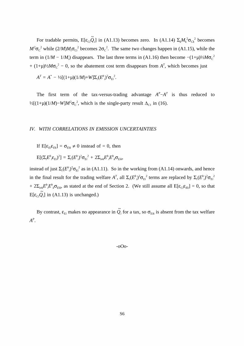
For tradable permits, E[εCiQ~

i] in (A1.13) becomes zero. In (A1.14) ΣkMk2σCk

2 becomes

M2σC2 while (2/M)MiσCi

2 becomes 2σC2. The same two changes happen in (A1.15), while the

term in (1/M − 1/Mi) disappears. The last three terms in (A1.16) then become −(1+µ)½MσC2

+ (1+µ)½MσC2 − 0, so the abatement cost term disappears from AT, which becomes just

AT = A* − ½[(1+µ)(1/M)+W]Σi(Ebi)

2σEi2.

The first term of the tax-versus-trading advantage AP−AT is thus reduced to

½[(1+µ)(1/M)−W]M2σC2, which is the single-party result ∆C1 in (16).

IV. WITH CORRELATIONS IN EMISSION UNCERTAINTIES

If E[εEiεEk] = σEik ≠ 0 instead of = 0, then

E[(ΣiEbiεEi)

2] = Σi(Ebi)

2σEi2 + 2Σi≠kE

biE

bkσEik,

instead of just Σi(Ebi)

2σEi2 as in (A1.11). So in the working from (A1.14) onwards, and hence

in the final result for the trading welfare AT, all Σi(Ebi)

2σEi2 terms are replaced by Σi(E

bi)

2σEi2

+ 2Σi≠kEbiE

bkσEik, as stated at the end of Section 2. (We still assume all E[εCiεEk] = 0, so that

E[εCiQ~

i] in (A1.13) is unchanged.)

By contrast, εEi makes no appearance in Q~

i for a tax, so σEik is absent from the tax welfare

AP.

-oOo-

S6