Tax Bases, Tax Rates and the Elasticity of

Reported Income

Wojciech Kopczuk

Department of Economics and SIPA, Columbia University, 420 West 118th Street,Rm. 1022 IAB, MC 3308, New York NY 10027 and NBER

Abstract

Tax reforms usually change both tax rates and tax bases. Using a panel of incometax returns spanning the two major U.S. tax reforms of the 1980s and a number ofsmaller tax law changes, I find that the elasticity of income reported on personalincome tax returns depends on the available deductions. This highlights that thiskey behavioral elasticity is not an immutable parameter but rather that it can be tosome extent controlled by policy makers. One implication is that base broadeningreduces the marginal efficiency cost of taxation. The results are very similar for allincome categories indicating that the rich are more responsive to tax rates becausetax rules that apply to them are different (their tax base is narrower). The pointestimates indicate that the Tax Reform Act of 1986 reduced the marginal cost ofcollecting a dollar of tax revenue, with roughly half of this reduction due to thebase broadening and the other half due to the tax rate reduction. As a by-product,the analysis in this paper offers a reconciliation of disparate estimates obtained byprevious studies of the tax responsiveness of income.

Key words: personal income tax, taxable income elasticity, tax complexityJEL classification: H2, H24, H31, J22, K34

1 Motivation

Complexity is often considered to be an undesirable feature of the tax system, but thisis usually postulated rather than derived from an economic model and its relationshipto other criteria for evaluating tax policy is unclear. A recent paper of Slemrod andKopczuk (2002) provides a specific framework for analyzing the cost of complexity inthe tax system by interpreting it in terms of the income tax base. A simple income

Email address: wkopczuk@nber.org (Wojciech Kopczuk).

Forthcoming in Journal of Public Economics 8 December 2004

tax is characterized by few deductions and, therefore, a broad tax base. Broadeningthe tax base increases revenue and affects administrative costs, but more subtly itmay also affect the excess burden of taxation: in their model, a broader tax base isassociated with a lower elasticity of taxable income and therefore with lower excessburden. Thus, in that framework, simplicity of the tax system directly affects theefficiency cost of taxation.

In this paper, I evaluate the empirical validity of such arguments by estimating theimpact of the tax base, measured as a fraction of income subject to taxation, onthe elasticity of income reported on personal tax returns. This elasticity is the keyparameter necessary to evaluate the deadweight loss of the income tax. My resultshighlight though that it is not a structural parameter depending only on underlyingpreferences and technology, but instead it depends on a non-rate aspect of the taxsystem (tax base) that can be manipulated by policy makers. This effect is not justtheoretically possible, it also turns out to be empirically relevant. Consequently, theresults indicate that the marginal deadweight loss of taxation can be controlled bypolicy makers. In particular, and as an illustration, I can assess potential efficiencygains resulting from a change to a broad-base low-rate tax system.

2 Context

The central importance of the elasticity of taxable income for public finance questionsfollows from two simple realizations. First, by the envelope theorem, the marginal taxrate (t) affects welfare of an individual in proportion to her taxable income (I). Theanalytics of the response are irrelevant. Second, with just income taxation in place,the marginal effect on revenue is dR

dt= t∂I

∂t+ I, again depending only on the total

taxable income. Therefore, having a measure of responsiveness of I is crucial for anyattempt to measure the efficiency cost of income taxation. 1 What is the relevantI? The traditional approach was to define I ≡ wL, where w is the wage rate andL is labor supply. Under this assumption, the elasticity of labor supply can be usedin place of the elasticity of taxable income. Apart from disregarding capital incomesubject to income taxation, this approach also ignores other potentially importantresponses to taxation such as effort, tax avoidance, tax evasion and income shifting.

In order to address this concern, following Lindsey (1987) and Feldstein (1995), theliterature has concentrated directly on income reported on tax returns (Auten andCarroll, 1999; Carroll, 1998; Goolsbee, 1999; Long, 1999; Sillamaa and Veall, 2001;Aarbu and Thoreson, 2001; Gruber and Saez, 2002). 2 Several authors argued thatchanges in the definition of taxable income provide an additional source of identifica-

1 See Feldstein (1999) and Slemrod (1998) for discussions of this argument and its limita-tions.2 See Slemrod (1998) for a critical discussion of this literature.

2

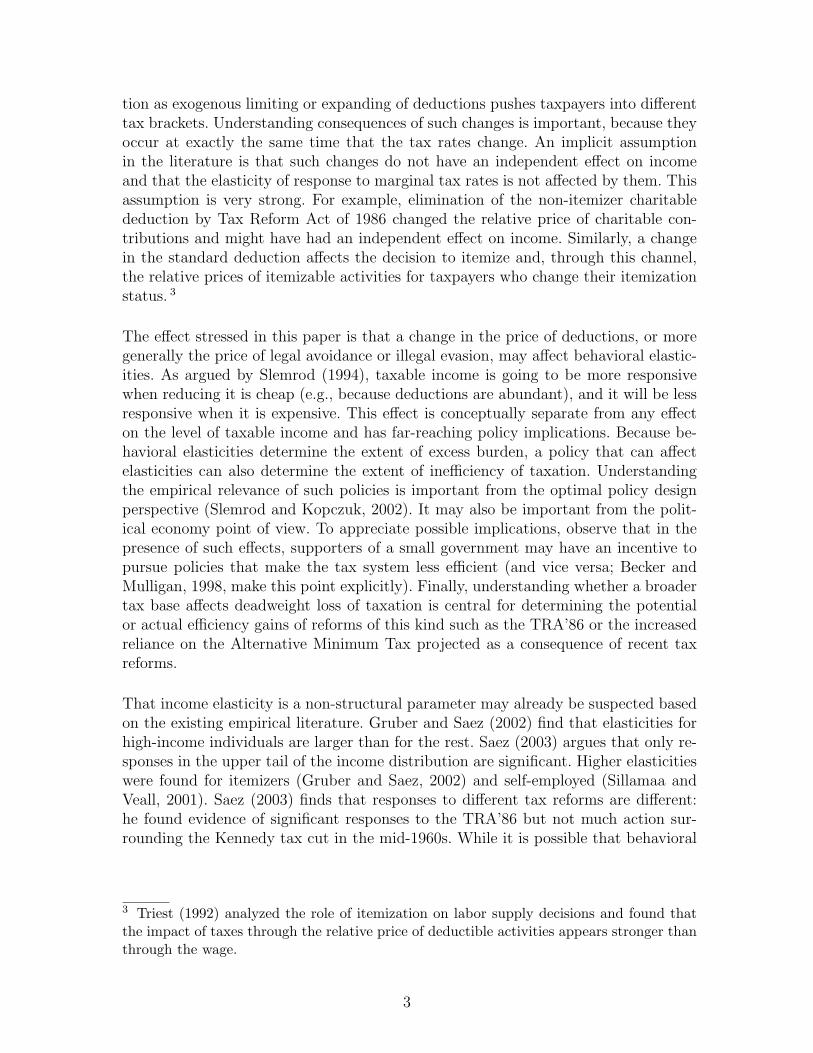
tion as exogenous limiting or expanding of deductions pushes taxpayers into differenttax brackets. Understanding consequences of such changes is important, because theyoccur at exactly the same time that the tax rates change. An implicit assumptionin the literature is that such changes do not have an independent effect on incomeand that the elasticity of response to marginal tax rates is not affected by them. Thisassumption is very strong. For example, elimination of the non-itemizer charitablededuction by Tax Reform Act of 1986 changed the relative price of charitable con-tributions and might have had an independent effect on income. Similarly, a changein the standard deduction affects the decision to itemize and, through this channel,the relative prices of itemizable activities for taxpayers who change their itemizationstatus. 3

The effect stressed in this paper is that a change in the price of deductions, or moregenerally the price of legal avoidance or illegal evasion, may affect behavioral elastic-ities. As argued by Slemrod (1994), taxable income is going to be more responsivewhen reducing it is cheap (e.g., because deductions are abundant), and it will be lessresponsive when it is expensive. This effect is conceptually separate from any effecton the level of taxable income and has far-reaching policy implications. Because be-havioral elasticities determine the extent of excess burden, a policy that can affectelasticities can also determine the extent of inefficiency of taxation. Understandingthe empirical relevance of such policies is important from the optimal policy designperspective (Slemrod and Kopczuk, 2002). It may also be important from the polit-ical economy point of view. To appreciate possible implications, observe that in thepresence of such effects, supporters of a small government may have an incentive topursue policies that make the tax system less efficient (and vice versa; Becker andMulligan, 1998, make this point explicitly). Finally, understanding whether a broadertax base affects deadweight loss of taxation is central for determining the potentialor actual efficiency gains of reforms of this kind such as the TRA’86 or the increasedreliance on the Alternative Minimum Tax projected as a consequence of recent taxreforms.

That income elasticity is a non-structural parameter may already be suspected basedon the existing empirical literature. Gruber and Saez (2002) find that elasticities forhigh-income individuals are larger than for the rest. Saez (2003) argues that only re-sponses in the upper tail of the income distribution are significant. Higher elasticitieswere found for itemizers (Gruber and Saez, 2002) and self-employed (Sillamaa andVeall, 2001). Saez (2003) finds that responses to different tax reforms are different:he found evidence of significant responses to the TRA’86 but not much action sur-rounding the Kennedy tax cut in the mid-1960s. While it is possible that behavioral

3 Triest (1992) analyzed the role of itemization on labor supply decisions and found thatthe impact of taxes through the relative price of deductible activities appears stronger thanthrough the wage.

3

elasticities vary with some personal characteristics, 4 it is also possible that differencesin behavior result from differences in the tax and institutional environment faced bydifferent individuals.

To address this issue, I concentrate on a broad measure of income and control forboth changes in tax rates and rules. Measuring rules is by itself difficult and a furtherproblem from the econometric point of view is to have enough variation in any suchmeasure to credibly identify the potential effects. In practice, time-variation alone isunlikely to provide such a variation. The model presented in the paper (Section 3)introduces and justifies a quantifiable measure of the non-rate aspects of the taxsystem in place that varies both over time and in the cross-section. The idea is to usethe tax base as a summary statistic for tax rules in place. I rely on a taxpayer-specificmeasure of the size of the tax base: the ratio of income that is subject to taxationto total income. This is an easily observable quantity that is affected by tax reformsin a mechanical way (although it of course varies also due to endogenous taxpayers’responses). Tax reforms induce variation in both tax rates and tax bases and thereforeprovide an opportunity to separately identify the two effects.

A few clarifications are in order at the outset. First, my broad income is a measureof all kinds of income reported on tax returns that can be consistently observed overtime. Using taxable income instead would be preferred from the theoretical pointof view. Such a measure is easy to obtain; however, because its definition changesfrequently, it is more difficult to incorporate in the analysis. In this paper, I mainlyestablish sensitivity of broad income to the size of the tax base. I discuss difficultiesinvolved in analyzing taxable income and show some basic results in Section 6.1.Second, the estimated response to the tax base reflects the degree of substitutabilitybetween (broad) income and deductible commodities. This intuition will be madeexplicit by the theoretical model of Section 3. Previewing the results, they indicatethat broad income and deductible commodities are substitutes so that a decrease inthe price of deductible commodities (higher tax rate) leads to a significant reductionin the level of broad income. Third, as in other papers in this literature, the majorlimitation of this approach is due to its focus on personal income only. For the overallefficiency cost of the tax system, one should also understand shifting between personaland other tax bases. It will be argued below, however, that the results are remarkablystable across different income categories that are likely very diverse in terms of theability to pursue the corporate income tax avoidance avenue. As a result, it appearsunlikely that the overall response would be significantly affected by this consideration.

The outline of this paper is as follows. In the next section, I describe a simple modelthat highlights the role of the tax base and underlies the empirical specification. Ipresent details of the empirical implementation and discuss the data in Section 4. I

4 For example, individuals with a relative preference for tax avoidance may choose ca-reers facilitating avoidance, such as self-employment. Kopczuk (2001) analyzes optimal taximplications of such behavior.

4

argue that different sample definitions explain differences in the results found in theprevious literature and provide baseline results without controlling for the tax baseeffects in Section 5. Following this discussion, I present my estimates of the elasticityof income and the strength of its dependence on the tax base (Section 6) and anextension to taxable income (Section 6.1).

The major contributions of this analysis lie in demonstrating that the elasticity ofreported income varies systematically with the tax base and that this effect is quan-titatively important. It also turns out that the results are similar for different incomecategories suggesting that the major aspects of tax environment relevant for tax-payers’ decision are appropriately controlled for. The final section discusses someimplications of these results.

3 Income Response to Tax Base Changes

In this section, I present the model underlying the empirical specification that follows.Intuitively, the number of deductible commodities (G) should have implications forthe responsiveness of income to the tax rate: marginal tax rate determines tax wedgebetween income and deductible commodities thereby inducing substitution responses.The importance of these response depends on the extent of deductibility and its inter-action with the marginal tax rate. This suggests an empirical specification in whichboth the tax rate and its interaction with G are controlled for. However, measuring Gexplicitly is not practical. To motivate the proposed solution, consider the followingmodel. Let Di, i = 1, · · · , N be various types of consumption. Assume that the utilityfunction is separable between these goods and determinants of broad income (suchas labor supply), and that the utility from consumption is given by v(D1, · · · , DN),where v(·) is “symmetric”, so that the order of Di’s does not matter for the value ofutility. 5 Denote the generic relative price of broad income B by w and the price ofgood i by pi. To simplify the notation, assume that in the absence of taxes all pricesare equal to 1. Expenditures on G (G < N) commodities are deductible from income.Because of the symmetry, deductions may be taken to be the first G commodities.Then, the after-tax prices are given by w = τ ≡ 1 − t, pi = τ for i ≤ G and pi = 1for i > G. The demand for B is a function of all prices and the non-earned income.The elasticity of B with respect to the net-of-tax rate has to reflect the impact of allrelative prices that are affected by the change. In order to incorporate nonlinear taxschedules, I additionally allow for varying virtual income R (so that the response toR represents the income effect). Thus,

5 Formally, it is assumed that for any vector D and its permutation P (D), v(D) = v(P (D))

5

∆ ln(B)∣∣∣∣∆R,∆τ

≈(

∂ ln(B)

∂ ln(w)+

G∑i=1

∂ ln(B)

∂ ln(pi)

)∆ ln(τ) +

∂ ln(B)

∂R∆R

=

(∂ ln(B)

∂ ln(w)+ G

∂ ln(B)

∂ ln(p1)

)∆ ln(τ) +

∂ ln(B)

∂R∆R . (1)

The last step makes use of the assumed symmetry of all deductible commodities. Thisformula depends on G, the number of deductible commodities which is unlikely to beobserved. However, using the Slutsky identity, symmetry of the Slutsky matrix andp1 = τ = w yields

∆ ln(B)∣∣∣∣∆R,∆τ

≈(

∂ ln(B∗)

∂ ln(w)+

GD1

B

∂ ln(D∗1)

∂ ln(w)

)∆ ln(τ)+

∂ ln(B)

∂R

[∆R+∆τ(B−GD1)

],

(2)where the superscript “∗” denotes the compensated effect. The first two terms formthe compensated elasticity of B with respect to the tax rate: it depends on theelasticity with respect to own price w as in the standard analysis, but it also dependson the cross elasticity of deductible goods with respect to w multiplied by the shareof deductible goods.

So far, a response to changes in G was ignored. However, it may be analyzed in asimilar manner. Consider an increase in G by ∆G (the case of a decrease would beanalyzed identically). It corresponds to prices of goods G + 1 to G + ∆G falling from1 to τ . Therefore, assuming that ∆G is small relative to N ,

∆ ln(B)∣∣∣∣∆G

≈G+∆G∑i=G+1

∂ ln(B)

∂ ln(pi)(ln(τ)− ln(1)) ≈ ∂ ln(B)

∂ ln(pG+1)ln(τ)∆G (3)

≈ ∂ ln(B)

∂ ln(p1)ln(τ)∆G =

∂ ln(D∗1)

∂ ln(w)

D1∆G

Bln(τ)− ∂ ln(B)

∂RtD1∆G .

Combined equations 2 and 3 characterize the response of broad income to a changein tax environment. To express it succinctly, define γ ≡ GD

B. Then, when evaluated

at the original point, ∆(γ ln(τ)) = D∆GB

ln(τ) + γ∆ ln(τ). Consequently, the responseof B is given by

∆ ln(B) =∂ ln(B∗)

∂ ln(w)∆ ln τ +

∂ ln(D∗)

∂ ln(w)∆(γ ln(τ)) +

∂ ln(B)

∂R

[∆R−∆T

], (4)

where ∆T is a change in the tax liability.

This analysis has two important implications. First, the response to tax changesdepends on G. Second, the impact of deductions is measured by the cross-elasticityand it is proportional to the (observable) share of deductions in the total incomeγ ≡ GD

B. This suggests using a natural specification where one controls for both the

tax rate and its interaction with the share of deductible commodities, attempting to

identify both ∂ ln(B∗)∂ ln(w)

and∂ ln(D∗

1)

∂ ln(w). Of course, γ is endogenous but it also reflects the

6

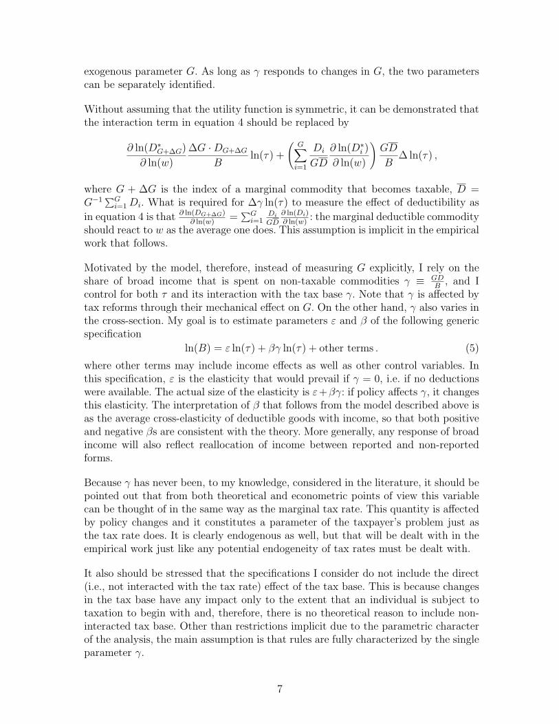
exogenous parameter G. As long as γ responds to changes in G, the two parameterscan be separately identified.

Without assuming that the utility function is symmetric, it can be demonstrated thatthe interaction term in equation 4 should be replaced by

∂ ln(D∗G+∆G)

∂ ln(w)

∆G ·DG+∆G

Bln(τ) +

(G∑

i=1

Di

GD

∂ ln(D∗i )

∂ ln(w)

)GD

B∆ ln(τ) ,

where G + ∆G is the index of a marginal commodity that becomes taxable, D =G−1∑G

i=1 Di. What is required for ∆γ ln(τ) to measure the effect of deductibility as

in equation 4 is that ∂ ln(DG+∆G)∂ ln(w)

=∑G

i=1Di

GD

∂ ln(Di)∂ ln(w)

: the marginal deductible commodityshould react to w as the average one does. This assumption is implicit in the empiricalwork that follows.

Motivated by the model, therefore, instead of measuring G explicitly, I rely on theshare of broad income that is spent on non-taxable commodities γ ≡ GD

B, and I

control for both τ and its interaction with the tax base γ. Note that γ is affected bytax reforms through their mechanical effect on G. On the other hand, γ also varies inthe cross-section. My goal is to estimate parameters ε and β of the following genericspecification

ln(B) = ε ln(τ) + βγ ln(τ) + other terms . (5)

where other terms may include income effects as well as other control variables. Inthis specification, ε is the elasticity that would prevail if γ = 0, i.e. if no deductionswere available. The actual size of the elasticity is ε+βγ: if policy affects γ, it changesthis elasticity. The interpretation of β that follows from the model described above isas the average cross-elasticity of deductible goods with income, so that both positiveand negative βs are consistent with the theory. More generally, any response of broadincome will also reflect reallocation of income between reported and non-reportedforms.

Because γ has never been, to my knowledge, considered in the literature, it should bepointed out that from both theoretical and econometric points of view this variablecan be thought of in the same way as the marginal tax rate. This quantity is affectedby policy changes and it constitutes a parameter of the taxpayer’s problem just asthe tax rate does. It is clearly endogenous as well, but that will be dealt with in theempirical work just like any potential endogeneity of tax rates must be dealt with.

It also should be stressed that the specifications I consider do not include the direct(i.e., not interacted with the tax rate) effect of the tax base. This is because changesin the tax base have any impact only to the extent that an individual is subject totaxation to begin with and, therefore, there is no theoretical reason to include non-interacted tax base. Other than restrictions implicit due to the parametric characterof the analysis, the main assumption is that rules are fully characterized by the singleparameter γ.

7

4 Data and Empirical Strategy

The data used in this paper comes from a panel of tax returns. Before it is describedin Section 4.2, I briefly discuss prior approaches to identifying the effect of taxeson taxable income focusing on my proposed modifications, including those necessaryto simultaneously identify the effect of the tax base. The identification problemsin this setup have been discussed extensively by Moffitt and Wilhelm (2000). Theimpact of unobservable demographic characteristics whose effect stays constant overtime and that are time-invariant can be eliminated by first-differencing the regressionspecification. Therefore, indexing individuals by i and denoting the time index by s,I specify my model in the first-differenced form as

∆ ln(Bis) = ε∆ ln(τis)+β∆[γis ln(τis)]+η∆ ln(Bis−Tis)+∆δvZvi +δh∆Zh

s +∆θis , (6)

where τ is the marginal net-of-tax rate, γ is the share of deductible consumption, T isthe total tax liability and Z = [Zh, Zv] is the vector of other relevant characteristics.The objective is to directly estimate the elasticity with respect to the net-of-tax rateτ ≡ 1 − t. As discussed above, the tax elasticity may depend on deductions andtherefore the coefficient on ln(τ) is allowed to depend on γ. This is the minimalextension of specifications considered in the prior literature that allows for testingthe constancy of the elasticity. The parameter ε is the broad income tax elasticitywhen γ = 0, that is for the comprehensive tax base. Equivalently, this is the responseof broad income motivated by substitution away from items reported on the taxreturn toward leisure, fringe benefits and other types of income. One can test whetherβ = 0, in which case there is a single tax elasticity. In principle, depending on whetherdeductible goods are substitutes or complements for the broad income, both positiveand negative β’s are consistent with the theory. The parameter η measures the incomeeffect. Finally, Zv is the set of time-invariant variables whose effect changes over timeand Zh is the set of time-specific variables whose effect stays constant over time.

All reported regressions include dummies for the single marital status, sex (these areZv’s) and the full set of year effects (Zh). The dataset contains no age informationother than age exemption for those older than sixty-five, but observe that linear ageeffects are controlled for by including year dummies in the first-differenced specifica-tion. The effect of any other variables is not controlled for and they are subsumed inthe ∆θ term.

4.1 Endogeneity and Instruments

As in any econometric analysis of the impact of taxes on income or labor supply, onehas to worry about endogeneity of the key right-hand side variables. Both the marginaltax rate and the tax base depend on a realization of income. The tax rate is the directfunction of the total income. The tax base is not a direct function of income, but it

8

may depend on it. Furthermore, given that only limited demographic information ispresent in the dataset, one has to worry about any systematic relationship of omittedvariables that are relevant for income with the tax base. For example, people withtemporarily high income may be willing to invest more in tax avoidance. On the otherhand, people with temporarily low income due to, e.g., medical conditions will havea lower tax base as they qualify for the medical deduction. The tax base is, similarlyas the marginal tax rate, an endogenous time-varying variable, exogenously affectedby policy shocks.

To consistently estimate ε and γ, what is necessary are instruments for ∆ ln(τis) and∆{γis ln(τis)} that are uncorrelated with ∆θis. I construct and use as my instrumentschanges in values of ln(τ) and γ ln(τ) absent any change in behavior (which I referto as “predicted” changes). 6 Only information as of time s is used to construct thepredictions of the time s+1 variables. In other words, the predicted tax base and thepredicted marginal tax rate differ from the original ones only to the extent that therewere changes in tax law. This eliminates the effect of behavioral response betweentime s and time s + 1, although it still leaves the individual-specific component. Inconstructing the predicted tax base, I account for changes in the medical deduction, 7

changes in the tax treatment of charitable contributions by non-itemizers (a deductionwas present between 1982 and 1986), deductibility of interests on personal debt thatwas phased out after 1986, changes in the IRA limits, the elimination of the second-earner deduction by TRA86 and the change in the treatment of moving expenses(the TRA’86 changed their status from an adjustment to an itemized deduction). Asa part of the process, the predicted itemization status is determined by comparingpredicted deductions with the corresponding standard deduction. All calculations areCPI-adjusted and thus account for changes in itemization incentives due to “bracket-creep.” Performance of the predicted tax base is illustrated in Figure 1 using the 1985data to predict the 1988 values (this change is mostly due to the Tax Reform Act of1986).

The marginal tax rate instrument is constructed analogously. I adjust all period squantities for inflation and compute the period s measure of taxable income account-ing for changes in its definition. The new itemization status is predicted and thenew tax schedule is applied to the result. 8 The income instrument is constructed as

6 In general and apart from the orthogonality assumptions, with just two years of datawhat is required for identification of both parameters is that the effect of at least two ofthe variables used in computing the marginal tax rate and tax base stayed constant overtime so that they don’t enter specification (6). With multiple years of data and multiple taxreforms, this assumption can be somewhat weakened: I can still identify the effect if trendsby at least two characteristics stayed constant over time.7 Until 1982, medical expenses above 3% of AGI were deductible, until 1986 - above 5%,after 1987 - above 7.5%. There were minor changes regarding how health insurance affectsthe calculation in 1982 and 1983.8 The results are not sensitive to a few other ways of constructing the tax rate instrument.For example, neither using inflated first-period capital gains as a component of the predicted

9

in Gruber and Saez (2002): it is simply ln(Bs − T Ps /ps+1) − ln(Bs − Ts) where Ts is

tax liability in period s, T PS is the tax liability predicted for period s + 1 by applying

the tax law as of period s + 1 to the period-s values, and ps+1 is the inflation factorbetween periods 1 and 2. As was the case with the other two instruments, the incomeinstrument relies only on variables as of period one.

The tax rate is a function of taxable income, and demographic characteristics (suchas state of residence, marital status, number of dependents, or age). Effectively then,the tax rate is a function of broad income, the structure of deductions/adjustmentsand demographic characteristics. In constructing the predicted tax base I rely on tax-able income, deductions and tax adjustments. As a result, the tax base is affectedby individual-specific and transitory components present in each of them. Some ex-amples of such influences are tastes for charity (that affect charitable contributions),own health status (affecting medical deduction), home ownership (affecting real estatetax and home mortgage deductions), credit history (affecting personal interest deduc-tions) and unobservable income shocks (affecting state tax liability and, through thischannel, the itemization status). The effect of the tax base on income can be identifiedto the extent that at least some of these characteristics are either (1) time-invariantwith their effect staying constant over time or (2) they do not independently affectincome (in which case they need not be time-invariant). In either case, it impliesthat such characteristics can be excluded from equation 6. Determinants of the taxbase whose independent effect on income is not differenced out may be either due totransitory effects or group-specific trends. The consistency of estimates rests on theseeffects being appropriately controlled for, exactly as it does in the analysis of the taxrate effects. Many individual characteristics can be expected to fall in this category.For example, own health status is likely a determinant of the transitory componentof income while home ownership is likely closely related to permanent income andthe group-specific trend. I assume that the effect of unobservable person-specific de-terminants of deductions that do not stay constant over time is fully accounted forby transitory and permanent income controls

The earlier version of this paper (Kopczuk, 2003) contains a detailed discussion of theimportance of controlling for both transitory and income components of inequality.Because I rely on instruments constructed using information as of time s, I need toaddress their possible correlation with both the group-specific trend and the transi-tory income component. To do so, I include two kinds of controls. I control for theindividuals’ ranks in the income distribution by including the level of income for yearpreceding the first year of the difference (i.e., t− 1 income). 9 Due to reliance on year

income nor ignoring adjustments of the definition of income subject to taxation made adifference.9 I am grateful to an anonymous referee for suggesting this approach. The working paperversion of this article used instead income as of the first year of the panel (1979). Althoughmajor conclusions are unaffected by this change, the “t − 1” approach is likely to lead tomore consistent measures of the rank and transitory income because these measures do not“age” as the panel ages. In particular, it turns out that this approach makes results for

10

t−1 income, observations for the first year (1979) are automatically excluded from thesample used for estimation. I define the transitory income component as the differencebetween current and t−1 income. I experiment with 10-piece splines in logarithms ofboth the t−1 income and the “transitory” component to allow for potential nonlineareffects. Nonlinearity in the permanent component allows me to account for trends inincome varying across different income classes. In principle, the transitory componentcan be controlled for in a linear fashion. However, because my measure of temporaryincome is a proxy and therefore certainly includes a measurement error, allowing forhigher-order effects may aid in eliminating the residual correlation and the resultingbias.

4.2 Data

I use the Statistics of Income/University of Michigan panel of tax returns that wereselected every year between 1979 and 1990, according to the last four digits of thesocial security number. There are usual pros and cons of relying on tax return data: thedataset contains little demographic information, but it includes detailed informationabout tax returns. The latter is crucial here, because it allows for constructing ameasure of the tax base. 10

I follow Gruber and Saez (2002) in comparing differences between observations threeyears apart. In other words, when differencing, I subtract observations for 1980 (1981,1982,...,1987) from the corresponding observations for 1983 (1984, 1985,...,1990). Thethree year spread was also used by Feldstein (1995). Using a longer spread allowsfor estimating permanent elasticities, while short-term differences can be significantlyaffected by income shifting over time. Using a much longer spread would confoundeffects of ERTA’81 and TRA’86 that were just five years apart. For example, thefour-year window would include the 1982-1986 pair that adjoins both of the majortax reforms.

The panel is not balanced. There are almost 300, 000 observations that translateinto close to 100, 000 three-year differences, but not all observations are used in theanalysis. I use only observations of individuals who are observed in year t − 1 andwhose marital status in years t − 1, t and t + 3 is identical. There are 59,006 suchobservations. Additionally, I exclude those who claim age exemption in either of thetwo years (9,309), those filing as the “head of household” (5052), those with non-positive income in t−1 or either year of the pair (776), those whose state of residence

single individuals somewhat more stable than when 1979 income is used.10 The predicted change in tax base is used as an instrument for tax base, but there is noinformation to construct predictions of new deductions. An instrument relying only on thepre-existing deductions is a valid instrumental variable if it remains correlated with actualtax base.

11

is unknown (20) 11 and some tax returns with missing data. This procedure leaves43,839 differenced observations.

I construct and use as the dependent variable the measure of broad income consistingof almost all income that had to be reported every year, regardless of whether itwas taxable or not. The only type of income that is excluded (following most ofthe previous studies) are realized capital gains. This is due to the lump-sum patternof their realizations. An extension of the analysis to taxable income is discussed inSection 6.1. Further details are in the appendix of the working paper version.

Tax rates and liabilities were computed by applying the NBER TAXSIM 12 calculatorto the actual taxable income (in particular, deductions are taken into account). Bothstate (ts) and federal income (tf ) tax rates are used. The effective marginal tax rateis calculated as tf (1 − ts) + ts for itemizers who claim state tax deductions and astf + ts for all others.

Spending on deductible commodities is defined to include total adjustments to income,total deductions (with the exception for state and local taxes) for itemizers, charitabledeductions for non-itemizers between 1982 and 1986 and non-taxable but reportedcomponents of income (such as the non-taxable part of unemployment insurance). Thevalue of γ is defined as the ratio of such spending to the broad income measure. Notethat, consistently with the model described earlier, the inelastic personal exemptionsand the standard deduction are not a part of the definition of γ. For the purposeof constructing γ, deductions need not be enumerated, because the tax base canbe mechanically constructed by dividing the taxable income observed on the returnthrough a measure of the broad income. The extent and sources of variation in γ willbe discussed in what follows.

Table 1 shows basic summary statistics for the sample used in estimation. The averagereported income is about $40,600 dollars, compared to the average initial income ofabout $39,394 dollars. 38% of the population is single and 46% of the sample itemizes.The average marginal tax rate for the whole sample is 25.3% in period 1 and 24.1% inperiod 2, while the tax base (1− γ) in both periods is on average the same at about0.87.

11 There is a small number of predominantly rich taxpayers whose state of residence is notreported in the dataset (for confidentiality reasons). For most of them, I do have informationabout their state of residence in one of the prior years and this is what I use, implicitlyassuming that they have not relocated in the meantime.12 The calculator is available at http://www.nber.org/taxsim/ and described in Feenbergand Coutts (1993).

12

4.3 Variation in the tax base.

There are two major aspects of the tax system that are responsible for determiningthe broadness of the tax base. First, deductions and adjustments explicitly excludeparts of income from taxation. As they vary, the tax base of the taxpayer varies.Second, tax bases of itemizers and non-itemizers are different. Changes in both thestandard deduction and the availability of itemized deductions affect relative payoffsfrom different itemization regimes. Therefore, they affect the itemization status evenwithout other behavioral responses.

Importantly, effects of such changes also vary cross-sectionally. Changes in the stan-dard deduction affect itemization status (and therefore the tax base) only of thosewhose gains from itemization are small enough. The elimination of the charitablededuction for non-itemizers affected the tax base of people making charitable contri-butions but not others. Changes in medical deduction affect itemizers who have highenough medical expenses. These effects can interact suggesting that tax base effectsare not simple functions of income (and, therefore, aiding in identification). For ex-ample, following the repeal of the non-itemizer deduction for charitable contributions,a non-itemizer may (but need not) change the itemization status. Without a change,the tax base would increase. If the itemization status changes, the tax base wouldlikely fall as deductions available to itemizers are taken advantage of.

Table 2 presents descriptive statistics showing the degree of variation of the key vari-ables over the years for the whole sample (this table is based on more observationsthan actually are used in the estimation). The temporal pattern indicates that tax re-forms of the 1980’s affected the tax base. The tax base was falling before 1986 and wassharply increased by the Tax Reform Act of 1986. Columns 7 and 8 show that similarpatterns are present for both itemizers and non-itemizers. The proportion of itemizersfell sharply following the TRA’86. If only the standard deduction had changed, theremaining itemizers would be people with relatively small tax bases. Nevertheless, theaverage tax base among itemizers increased indicating that these changes were notsimply caused by changes in the standard deduction but also involved elimination ofsome of deductions.

Column 8 of Table 2 shows that non-itemizers do not automatically have γ equal zero(the tax base equal to one), 13 although it is not far from that. The tax base of non-itemizers was on average lower following the ERTA’81 mostly due to the availability ofa deduction for charitable contributions by non-itemizers. The cross-sectional changesare illustrated in Figure 2. It shows the distribution of the tax base in 1980, 1982,1985 and 1988 (only individuals in the sample used for estimation are included). Inevery year, the distribution is bimodal corresponding to groups of itemizers and non-

13 Observe that the standard deduction and dependent exemptions do not enter the defi-nition of γ. Subtractions from the broad income in the numerator of γ include only itemsthat can be adjusted by taxpayers.

13

itemizers. The ERTA’81 shifted the whole distribution to the left, while the TRA’86shifted it back to the right. 14

5 Results — Tax Rate Effect Only

I begin by considering specifications without the interaction of the marginal tax rateand the tax base. By doing so, I am able to identify the source of differences in previousstudies and present directly corresponding estimates obtained using my approach.These estimates serve as a reference point for the discussion of the role of tax base inthe next section.

Income controls. In order to highlight the importance of the choice of income con-trols, I present in Table 3 estimates of the net-of-tax coefficient (i.e., the coefficienton ∆ ln(τ) ≡ ∆ ln(1 − t)) using the full sample and various means of income con-trols. 15 , 16 The first specification excludes income controls and leads to a significantnegative coefficient. The following two specifications are as in Gruber and Saez (2002):controlling for the current income has a huge impact, but allowing for nonlinearitiesreduces the estimated elasticity to about 0.15. The same result was obtained by Gru-ber and Saez (2002).

The following four specifications highlight the importance of both permanent andtransitory components of income. The effect of the permanent component is sensitiveto nonlinearities. Allowing for a nonlinear effect in t − 1 income or controlling forjust the transitory component has relatively little impact on the estimated elasticity,which remains significantly negative. The last panel allows for both types of incomecontrols entering in different combinations of linear and nonlinear effects. Allowing fornonlinear effects in each case significantly reduces the estimated elasticity. When bothincome controls are allowed to enter in a nonlinear fashion, the estimated elasticity

14 Although I account for many changes in the tax base as discussed in Section 4.1, em-pirically the major source of variation in the tax base is due to changing incentives foritemization. In fact, none of the results in this paper would be affected in a major way if thetax base instrument was only accounting for the change in the itemization status, withoutadjustments for other changes in the definition.15 As discussed later, these specifications are not directly comparable to the results of Gruberand Saez (2002) and Auten and Carroll (1999), because these papers additionally restrictsamples used in estimation.16 All reported results come from the IV regressions. There is no evidence of the weakinstrument problem for the tax base and the tax rate instruments, although the incomeeffect instrument has low explanatory power in some specifications. Estimates are robust tonot controlling for the income effect. I report the Huber-White standard errors clustered byindividuals that are robust to non-independence of the error terms for the same individual(as well as heteroskedasticity).

14

is at 0.27 and significant. The final specification allows for year-specific nonlineartransitory controls, but this generalization has virtually no impact. 17

Sample Selection. As discussed above, it is important to control for the mean re-verting components of income. Apart from controlling for the current level of income,earlier papers also restricted their samples by excluding certain individuals with lowincomes. Gruber and Saez (2002) exclude “taxpayers whose income is below $10000in year 1 [in 1992 dollars], to avoid very serious mean reversion at the bottom ofthe income distribution.” Feldstein (1995) excludes taxpayers with tax rates below22 percent. Similarly, Auten and Carroll (1999) limit their sample to “taxpayers withincomes at or above the threshold for the 22% marginal tax rate in 1985.” Carroll(1998) excludes taxpayers with income below $50,000 in 1989 (approximately $56,000of 1992 dollars).

By relying on the realized tax rate, the selection rule used by Feldstein (1995)and Auten and Carroll (1999) excludes high income individuals with low taxableincome. These papers find larger elasticities than the other two papers that basetheir sample selection on the income directly. That this is not a coincidence is illus-trated in Table 4. I use the same dataset as Gruber and Saez (2002). This datasetconstitutes about 20% of the dataset used by Auten and Carroll (1999). The rest oftheir sample oversamples rich individuals and is not publicly available. They statethat they obtain very similar results when they limit the sample to the public subset(p. 692, footnote 2). They analyze the 1985-1989 difference only. Because the Feld-stein (1995) and Auten and Carroll (1999) restriction depends on the tax system inplace, I present the results for the 1985-1988 change only, using logarithm of incomein 1985 as a control for the mean reversion problem. 18 Coefficients estimated basedon the full sample are extremely large, suggesting that the mean reversion problemat the bottom of the distribution may be indeed important. Using the Auten andCarroll (1999) restriction to taxpayers with taxable income qualifying for at least22% tax bracket in 1985 brings the elasticity down to about 0.8. 19 The Gruber andSaez (2002) restriction to individuals with current income above $10K reduces theelasticity to less than 0.4, 20 while the further restriction to those with current in-come above $30K makes it essentially zero (with the sample size similar to the A-Cspecification). These results closely track the results obtained in the corresponding

17 The results for the subsample of married individuals are fairly similar and available fromthe author. The difference between results for the full sample and those for married indi-viduals only was much more pronounced in the working paper version when 1979 incomewas used to measure permanent income and to construct the transitory income. Althoughcontrolling for t− 1 income helps at this stage, it will be shown below that it does not solvesimilar problems when the tax base is controlled for.18 Auten and Carroll (1999) report results with log income control only.19 The Auten and Carroll (1999) estimate in the directly comparable specification is 0.67.20 An appendix available from the author contains a detailed discussion of the differencesin definitions of variables and sample selection between this paper and Gruber and Saez(2002).

15

papers: it appears that different sample choices played crucial role. Compared to thesedifferences, the effect of excluding older individuals and those subject to the AMT(cf. the first and second panels of Table 4) is minor. 21

Splitting the sample according to either current income or the marginal tax rate isinfluenced by transitory and permanent components of income as well as individualeffects. Additionally, splitting the sample according to the level of the tax rate isaffected by the itemization and tax avoidance behavior. If the parameter of interestis constant, the sample selection bias will be present to the extent that factors deter-mining selection are correlated with the error term and are not separately controlledfor. Were transitory and permanent components of income and other determinants ofselection appropriately controlled for, the sample selection bias should not be present.In that case, if the underlying parameter of interest is indeed constant, how the sam-ple is split should not affect the results, contrary to the results in Table 4. The resultsin that table suggest a misspecification. Although in principle it is possible that oneof such arbitrary restrictions will yield correct results, it is hard to defend a prioriany particular choice.

The decision to split the sample may also be motivated by the belief that the underly-ing parameters vary in population. This was likely an implicit motivation of previousresearch that did not consider the low-income group as a valid control for high-incomepeople who experienced the largest tax changes. Differences in behavior of the richand the poor can be ascribed to either tastes or technology. In the framework of thispaper, taste differences are accounted for by allowing for individual effects and thusshould not affect the results. Differences in available technology are allowed for bycontrolling for the tax base. The case for the elasticity of income to vary across dif-ferent groups is therefore weaker than in prior research. Therefore, I investigate howsensitive my estimates are to the sample selection and consider stability of estimatesas a testable prediction of the approach.

6 Results — Tax Rate vs. Tax Base

The previous section offered a mechanical explanation for the differences in resultsfound in previous papers. Relying on insights regarding the relevance of sample se-lection and income controls, I turn now to the main question: the impact of the tax

21 Although not reported here, including current income splines as in the preferred speci-fication of Gruber and Saez (2002) renders tax coefficients in all specifications in Table 4insignificant. With a single difference and just one tax change, allowing for nonlinearity inincome eliminates income as the source of identification. This is not a problem for Gruberand Saez (2002) and this paper, because with multiple years of data one need not rely onidentification off the cross-sectional variation in tax rates. However, this is the major sourceof identification in the context of Feldstein (1995) and Auten and Carroll (1999).

16

base on reported income.

The main results are shown in Table 5. For comparison purposes, the first specifica-tion shows results when only the tax rate is controlled for. The estimated elasticityfor the whole sample is .27 while estimates for subsamples are all smaller and usuallyimprecisely estimated. Estimates obtained by splitting the sample using t− 1 incomeappear larger than those obtained by splitting the sample according to the contempo-raneous income level. Results are sensitive to sample selection suggesting a possiblespecification error. The rest of the table contains results when both tax rate and taxbase are controlled for. Estimates for the whole sample indicate that both direct taxelasticity and tax base effects are important. The direct tax elasticity is 0.096 whilethe coefficient on γ ln(τ) is .789 and very significant. Evaluated at the average (in thesample used for estimation) tax base of 0.881 (i.e., γ = .119), this corresponds to thetax elasticity of 0.19. In the same sample, following the Tax Reform Act of 1986 theaverage tax base increased from 0.846 in 1986 to 0.900 in 1987, so that γ declinedfrom 0.154 to 0.100. Consequently, these point estimates imply that the elasticity ofbroad income at the average tax base fell from 0.217 to 0.175.

In the following column, the direct effect of the tax base is estimated. There is notheoretical argument for why the tax base should enter the specification directly —tax base matters only to the extent that it implies tax savings. Comfortingly, thedirect effect of the tax base is very close to zero, although it reduces the precision(though not point estimates) of the interaction coefficient. 22 The next seven columnsshow estimates in subsamples defined by either current or “permanent” income. Ineach case, the direct tax elasticity is insignificant, while the effect of interaction isusually large and close to estimates for the whole sample. These results suggest thatby allowing the tax base to affect the elasticity of response, the model is appropriatelycontrolling for heterogeneity in behavioral responses.

The next two panels of Table 5 show results by marital status. While one might arguethat variation in marital status variations provides an additional source of identifi-cation, this is a difficult point to make, because it implies that the same behavioralmodel applies to both types of households. Furthermore, single individuals are likelyto be predominantly young and therefore experiencing large changes in income fol-lowing completion of their education. Such reasoning led Auten and Carroll (1999)to exclude individuals younger than 25 from their sample. In the absence of moredetailed demographic information (in particular, having no information about age), Iam not able to control for such considerations explicitly. However, splitting the sam-ple by marital status allows for assessing the relevance of this problem if most of theyoung individuals are single.

Table 5 reveals that results for single and married individuals are quite different. The

22 The results for subsamples are more sensitive to the inclusion of the direct effect of the taxbase. Given a high degree of collinearity that it induces and the lack of economic argumentfor controlling for the tax base, I do not present these results.

17

results for singles are all over the map. Both estimates of the direct elasticity andthe interaction term vary widely in subsamples and are always insignificant. It makesit difficult to treat seriously the somewhat larger (but still statistically insignificant)estimates based on the whole sample of single individuals. It is very likely that manyindividuals in this group are working part-time or entering the labor force whilein the sample, so that changes in their income are not tax motivated. Given theinability to control for other demographic characteristics of these individuals, I believethat results for single individuals are not meaningful. The results for the sample ofmarried individuals are, however, remarkably stable. The direct tax elasticities arealways insignificant and close to zero. The effect of the interaction is quite preciselyestimated at 0.73 when all married individuals are included and this point estimateis within one standard error of estimates for each of the considered income groups.As was the case when the full sample was considered, the direct effect of the tax baseplays no role.

With very few exceptions, income effects are close to zero and insignificant.

A number of other specifications were considered (but are not reported here). The re-sults are quite similar (although somewhat more sensitive to the choice of the sample)when one controls for splines in current income (as in Gruber and Saez, 2002) ratherthan separately for “transitory” and “permanent” components. The results are notaffected by limiting attention to individuals who were observed in all years. Resultsare also very similar when one uses only differences starting between 1980 and 1982 toeliminate the Tax Reform Act of 1986 from the analysis or when using 1983-1987 toeliminate the ERTA’81 (though extensive controlling for income makes identificationbased on a single reform tenuous). Limiting attention to just 1980 and 1985 to avoidobservations adjacent to reforms results in point estimates that are insignificant, butwithin one standard error of the results based on the full sample.

6.1 Taxable Income

Focusing on broad income, I demonstrated that its elasticity is a non-trivial functionof tax policy. From the point of view of evaluating distortions of the tax system,broad income allows for a wider range of responses than traditional analysis focusingon labor supply. However, it falls short of measuring all tax motivated responses, asrequired by the taxable elasticity approach advocated by Feldstein (1999).

Given that a number of papers attempted an analysis of taxable income (e.g., Autenand Carroll, 1999; Gruber and Saez, 2002), it is worthwhile to discuss related prob-lems. Incorporating any consistently defined concept of income in the analysis isstraightforward and fits easily into the framework of this paper. This was the in-tention of approaches pursued in previous papers: taxable income was defined asbroad income minus consistently defined deductions and adjustments. However it is

18

important to recognize that in the presence of itemization decision (an importantconsideration in the United States) no deduction is in fact “consistently” observed:whether a researcher can observe it or not depends on the taxpayer’s itemization de-cision. 23 Denoting broad income as B, the consistent definition of deductions as D,the (reference level of) standard deduction as S and personal exemptions by E, allprevious papers defined taxable income as T ≡ B − max(D, S) − E. 24 Taxable in-come defined in this way is not a differentiable function of individual decisions: it hasa kink at D = S violating an implicit assumption underlying econometric approachesbased on a linear regression. It also introduces censoring of the residual present inD, potentially leading to a bias when estimating the response of taxable income. Forexample, consider an individual who chooses not to pursue certain deductions in re-sponse to a tax cut (e.g., because the relative price of charitable contributions rises)and therefore finds it non-profitable to itemize anymore. The response of his taxableincome on the margin should reflect a change in deductions. Consider estimating thetax coefficient. In the presence of a discrete tax change, the change in deductionswill be censored and the response will be understated. The bias for individuals whoswitch to itemization will go in the opposite direction. While these effects may cancelout (approximately 15% of individuals change their itemization status, with similarnumbers switching to and away from itemization), it is not an appealing assumptiona priori.

Even ignoring the censoring problem, the response for itemizers reflects the responseof B −D while the response for non-itemizers reflects the response of broad incomeonly. It is unlikely that B−D and B respond in the same way, after all the expectationthat these responses are not the same is the rationale for separately analyzing taxableand broad income. At best therefore, when only the marginal tax rate is controlledfor, this approach could be interpreted as discovering some form of the weightedaverage of the two types of responses. These weights will be related to the relativeimportance of itemizers and non-itemizers in identification and are therefore likely tobe sensitive to the reform and instruments considered. Controlling for the tax basewould help to alleviate this concern because it allows for the elasticity of response tovary with comprehensiveness of person-specific taxable income and therefore it allowsfor different elasticities for itemizers and non-itemizers.

Even without any behavioral response, taxable income would change when the item-ization decision changes as a result of altered rules. This problem has been recognizedbefore and it may be addressed using a constant definition of taxable income thatrelies on the least generous deduction regime, as in some of the previous papers. Evenunder a constant definition of taxable income, though, there may be responses of tax-able income that occur purely as the result of changes in rules without any changes intax rates. When a deduction is eliminated (in particular, it cannot then be included

23 Adjustments can be consistently observed but their quantitative importance is small.24 According to this definition, taxable income excludes tax-free standard deduction andpersonal exemption, both set at the level in a selected reference year.

19

in the least generous constant definition), a taxpayer may decide not to itemize any-more. This may entail scaling down of other deductions (included in the constantdefinition) that might have been large enough before so that they were deductibleunder the constant definition of income. As a result, the constant-definition taxableincome will respond without any change in tax rates. Because such changes occur atthe same time as tax changes, they may be confounded with tax effects. This effectwill not be picked up by year effects: it applies to a selected group of individuals,i.e. those who switch their itemization status. These individuals are, likely, locatedsomewhere in the middle of income distribution. The direction of the bias from thissource depends on its correlations with the instruments for marginal tax rate and taxbase changes. Finally, an approach using a “constant” definition of taxable incomeat best measures the response of the actual taxable income under just one particulartax regime that corresponds to the “constant” definition.

One can imagine approaches to addressing the responsiveness of taxable income byexplicitly modeling itemization decision and incorporating changes in observability ofdeductions in the econometric framework. Such an approach would be a major exten-sion of this paper and it would be a very interesting contribution to this literature.

In what follows, I present specification checks that are intended to assess the relevanceof concerns listed above. Table 6 contains the corresponding results. All regressionsinclude splines in permanent and transitory taxable income defined analogously asin the case of broad income. The results of basic regression with taxable income asa dependent variable and without the tax base is shown in the first column. Thisregression suffers from problems discussed above but, except for not restricting thesample by income level, it is analogous to the specifications estimated in previouspapers. The baseline estimate of the elasticity for the whole sample is 0.41, similar tothe Gruber and Saez (2002) estimate and smaller than the estimates in Auten andCarroll (1999). The elasticity for married individuals is somewhat smaller at 0.3. Thenext two columns present two specification checks intended to assess the importanceof problems due to switching itemization and censoring. In the first one, I eliminatethose individuals whose itemization status changed between the two years. Althoughthis is an endogenously selected group, this approach allows for assessing its quantita-tive importance for the results. In the following column, I rudimentarily control for theimpact of censoring by including the actual change in itemization status as a regres-sor. Eliminating individuals whose itemization status changed reduces the elasticity,while the censoring control has only a small impact on the results. The following threecolumns repeat the same exercises, this time weighting all regressions by individuals’taxable income. Consequently, these estimates reflect sensitivity of revenue (relevantfor tax policy evaluation) rather than individual behavioral parameters. This distinc-tion is important when there is heterogeneity in responses. In particular, it seems thatover-weighting high-income people results in higher estimated elasticity, suggestingthat perhaps they are more responsive to taxation.

In the second panel, the same experiments are repeated when the tax base is controlled

20

for. The basic regression indicates that the elasticity of response is sensitive to thetax base. Point estimates indicate both stronger sensitivity of the elasticity to thetax base and a stronger direct effect (based though on the comparison of insignificantcoefficients). Estimates of the elasticity evaluated at the mean value of γ (about 0.12)are lower than estimates based on the results without the tax base. These resultssuggest that there was a bias due to omitting the tax base effect. The following twoexperiments demonstrate the relevance of the itemization-switching problem. Bothremoving “switchers” and controlling for censoring leads to a much sharper effect ofthe tax base. The message is very similar in weighted regressions.

The large and significant interaction coefficient provides a strong evidence of hetero-geneity in responses to taxation. These results also raise concerns about results arisingwhen the tax base is not controlled for. Suppose that these results indeed reflectedthe average elasticity. In order to reconcile taxable income elasticity arising from thatapproach (panel one of Table 6) with structural results in the second panel, one needsγ of the order of 0.3 to 0.4 (depending on specification). In fact, though, the averageγ in the sample used for estimation is about 0.12 and the average income weighted γis just 0.16. Less than 12% of the sample have γ greater than .3 and only about 5%have γ greater than 0.4. Even among those with income over $100,000, there are just6% people with γ above 0.4. Consequently, high taxable income elasticities estimatedin the first panel are hard to reconcile with the structural approach.

This analysis suggests that taxable income is indeed sensitive to the tax base changes.It can be tentatively concluded that the elasticity of taxable income is more sensitiveto the tax base than it was the case with broad income. The specification checkspresented above suggest that proper estimation of the interaction coefficient requiresfurther work on addressing the issue of changes in the definition of taxable income.

7 Discussion and Implications

I interpret the results as indicating that, apart from the difficulty of controlling fortransitory and permanent shocks in income, previous studies suffered from two addi-tional problems. First, the model was mis-specified due to ignoring the effect of thetax base. Second, the results indicate that mixing individuals with different maritalstatus while identifying the effect of taxes on income is suspect (at least, given scarcedemographic information).

Table 5 contains the major results. Results for married individuals are consistentacross all considered specifications: the direct effect of the tax rate is small and in-significant while the interaction term is in most cases of the order of 0.7 and comfort-ably significant. The results based on the full sample are a bit less reliable, althoughthey also indicate that the interaction term plays an important role. Therefore, I con-centrate on the results for all married individuals in developing normative implica-

21

tions. The estimated direct tax elasticity of broad income is 0.003 while the estimatedeffect of the interaction with the tax base is 0.727. In the case of taxable income, thecorresponding (income weighted) results are 0.123 and 1.063. These results imply thatan individual who has no access to any deductions would not respond to changes inthe tax rates. The more deductions are available, the stronger the response.

Are these results reasonable? As highlighted by the theoretical model, the strengthof estimated response reflects the degree of substitutability of broad income anddeductible commodities. The estimated coefficient indicates that broad income anddeductible commodities are strong substitutes: a decrease in the price of deductiblecommodities (higher tax rate) leads to a significant reduction in the level of broadincome. Thus, for example, the results are consistent with lower prices of charitablecontributions or medical care leading to less labor supply and, therefore, less incomereported on the tax return. When the tax rate increases broad income responds fortwo reasons. First, there is a standard direct effect on determinants of broad incomethat now become costly. The finding of this paper is that this effect is close to zeroand this result is consistent with the consensus regarding inelasticity of labor supply.Second, there are indirect effects present: an increase in the tax rate reduces prices ofall deductible commodities. I find that broad income is reduced in response. Financ-ing the same level of cheaper deductions requires less income, and the finding is thatincome reported on tax returns falls. The elasticity of substitution is smaller than one(of the order of 0.7 to 0.8), suggesting that broad income is not reduced one for onewith the falling cost of deductions but that it is instead used for other purposes. Inparticular, there seems to be evidence that taxable income responds more stronglythan broad income so that deductible goods are responsive to tax rates as well. Theresponse of broad income can take many forms, but the importance of the interactionwith deductions is suggestive of reporting rather than real responses: additional in-come that could be potentially concealed/re-timed/unrealized is reported on the taxreturn if there is a corresponding deduction to be taken.

As Table 2 shows, the mean marginal tax rate for fell from 0.212 in 1985 to 0.184 in1988, while the mean average tax base increased from 0.880 to 0.926. The estimatedresults suggest therefore that the Tax Reform Act of 1986 reduced the elasticity ofreported income to the tax rate at the mean tax base from 0.09 to 0.06, while theresponsiveness of taxable income fell from 0.25 to 0.20. 25 There are two reasonsfor the change. First, the tax reform had a mechanical effect on the tax base, absentbehavioral response. Second, under the new tax environment taxpayers adjusted theirbehavior and, consequently, there has been some endogenous change in the tax base.The last effect could be present even if only tax rates changed but it would be ignoredby the standard analysis.

One simple implication of this result can be described by using the marginal cost of

25 I find no evidence to conclude that the income effect is different from zero, so thatcompensated and uncompensated income elasticities are assumed to be equal.

22

funds (MCF). The simple formula for the MCF of the linear income tax is MCF =1

1− t1−t

π, where t is the marginal tax rate and π is the elasticity of taxable income. I

proceed by replacing π by the estimate of the taxable income elasticity at the mean: ε+γβ . Evaluating this formula at the mean tax rates yields the 1985 value of the MCFof 1.072 and the 1988 value of 1.044. Interpreting these numbers, they imply that thesocial cost of collecting a dollar of revenue fell by 3 cents per dollar. Alternatively,given estimated null income response, it directly translates into a reduction in themarginal excess burden by 39%, from 0.072 cents per dollar to 0.044. Holding thetax base constant at the initial level, the same change in the marginal tax rate wouldhave reduced the MCF to just 1.060, resulting in the 60% smaller marginal excessburden reduction. While these are only suggestive calculations, they illustrate thepotential quantitative importance of understanding the role of non-tax instrumentsin evaluating the efficiency cost of tax policy.

These results also indicate that the elasticity of income may well be different fordifferent groups, to the extent that their tax bases are different. The results in Table 5indicate (using the average tax base in each group and estimates for the full marriedsample) that the elasticity of reported income for people below the $30,000 thresholdwas 0.088 while the corresponding elasticity for those with incomes above $100,000was 0.156. These differences are much smaller than found by Gruber and Saez (2002).Even though they still systematically vary with income, they do not necessarily implythat tax rates at high incomes need to be adjusted to account for stronger behavioralresponse: the differences in elasticities are themselves a function of policy. Finally,accounting for the tax base effects offers a positive framework for understandingdifferences in behavioral elasticities across countries: estimates for different countriesmay vary reflecting different tax systems in place.

To be sure, there are complicating factors that are not addressed in this paper andthat may be very relevant. To the extent that the estimated response merely reflectsshifting from other tax bases such as the corporate or capital gains tax, the elasticityof reported income should be supplemented by losses or gains of revenue from othersources. Accounting for such responses could undermine calculations performed above.

Additionally, the elasticity of income determines only the cost of taxation, while anycomplete analysis of policy requires understanding benefits as well. There may betrade-offs involved in the choice of tax base to the extent that deductions from thetax base are socially beneficial on, for example, redistributive grounds. Also, a broadertax base may feature different administrative costs (Yitzhaki, 1979; Wilson, 1989).

The bottom line is that any analysis of the cost of taxation should not ignore the factthat the crucial elasticity of taxable income is endogenous to the size of the tax baseand, more generally, to other aspects of tax system. Putting these results in a broaderperspective, this paper lends empirical support to the theoretical ideas advanced bye.g., Mayshar (1991); Slemrod (1994, 2001) and Slemrod and Kopczuk (2002). Thecost of taxation is not merely a function of marginal tax rates, consumer preferences

23

and technology, but rather it crucially depends on a broader tax environment and thestructure of tax policy. Therefore, economic analysis of the optimal tax policy has toincorporate tax avoidance and administration.

Finally, the non-tax-rate effect stressed in this paper can be relevant for any analysisof the effects of taxation on economic variables. As a general lesson, one should becareful when using tax reforms as natural experiments to identify the effect of taxationon economic variables. Such exercises usually assume that the elasticity of response isconstant, while major changes in the tax system are likely to invalidate this assump-tion: tax elasticities are fundamentally non-structural parameters. As demonstratedhere, acknowledging this issue does not necessarily eliminate usability of tax reformsas a source of variation, but it calls for a more comprehensive account of the changesthat they induce.

Acknowledgements

I am grateful to anonymous referees, David Green, Jon Gruber, Kevin Milligan, JoelSlemrod, seminar participants at UBC, Columbia, Berkeley, Stanford and the 2003meetings of the IIPF for comments on an earlier draft. I thank Emmanuel Saez forsharing his programs and the data and Daniel Feenberg for help with the TAXSIMprogram. Financial support from the Social Sciences and Humanities Research Coun-cil of Canada and the UBC Hampton Fund is gratefully acknowledged.

References

Aarbu, Karl O. and Thor O. Thoreson, “Income Responses to Tax Changes —Evidence from the Norwegian Tax Reform,” National Tax Journal, June 2001, 54(2), 319–334.

Auten, Gerald and Robert Carroll, “The Effect of Income Taxes on HouseholdBehavior,” Review of Economics and Statistics, November 1999, 81 (4), 681–693.

Becker, Gary S. and Casey B. Mulligan, “Deadweight Costs and the Size of Gov-ernment,” Working Paper 6789, National Bureau of Economic Research November1998.

Carroll, Robert, “Do Taxpayers Really Respond to Changes in Tax Rates? Evidencefrom the 1993 Act,” Office of Tax Analysis Working Paper 78, U.S. Department ofTreasury 1998.

Feenberg, Daniel R. and Elizabeth Coutts, “An Introduction to The TAXSIMModel,” Journal of Policy Analysis and Management, Winter 1993, 12 (1), 189–94.

Feldstein, Martin S., “The Effect of Marginal Tax Rates on Taxable Income: APanel Study of the 1986 Tax Reform Act,” Journal of Political Economy, June1995, 103 (3), 551–572.

24

, “Tax Avoidance and the Deadweight Loss of the Income Tax,” Review of Eco-nomics and Statistics, November 1999, 4 (81), 674–680.

Goolsbee, Austan, “Evidence on the High-Income Laffer Curve from Six Decadesof Tax Reforms,” Brookings Papers on Economic Activity, 1999, (2), 1–47.

Gruber, Jon and Emmanuel Saez, “The Elasticity of Taxable Income: Evidenceand Implications,” Journal of Public Economics, April 2002, 84 (1), 1–32.

Kopczuk, Wojciech, “Redistribution when Avoidance Behavior is Heterogeneous,”Journal of Public Economics, July 2001, 81 (1), 51–71., “Tax Bases, Tax Rates and the Elasticity of Reported Income,” Working Paper10044, National Bureau of Economic Research October 2003.

Lindsey, Lawrence, “Individual Taxpayer Response to Tax Cuts: 1982-1984, withImplications for the Revenue Maximizing Tax Rate,” Journal of Public Economics,July 1987, 33 (2), 173–206.

Long, James E., “The Impact of Marginal Tax Rates on Taxable Income: Evidencefrom State Income Tax Differentials,” Southern Economic Journal, April 1999, 65(4), 855–69.

Mayshar, Joram, “Taxation with Costly Administration,” Scandinavian Journal ofEconomics, 1991, 93 (1), 75–88.

Moffitt, Robert and Mark Wilhelm, “Taxation and the Labor Supply Decisionsof the Affluent,” in Joel Slemrod, ed., Does Atlas Shrug? The Economic Conse-quences of Taxing the Rich, New York: Harvard University Press and Russell SageFoundation, 2000.

Saez, Emmanuel, “Reported Incomes and Marginal Tax Rates, 1960-2000: Evidenceand Policy Implications,” August 2003. University of California-Berkeley, mimeo.

Sillamaa, Mary Anne and Michael R. Veall, “The effect of marginal tax rateson taxable income: a panel study of the 1988 tax flattening in Canada,” Journal ofPublic Economics, June 2001, 80 (3), 341–356.

Slemrod, Joel, “Fixing the Leak in Okun’s Bucket. Optimal Progressivity WhenAvoidance Can Be Controlled,” Journal of Public Economics, September 1994, 55(1), 41–51., “Methodological Issues in Measuring and Interpreting Taxable Income Elastici-ties,” National Tax Journal, December 1998, 51 (4), 773–788., “A General Model of the Behavioral Response to Taxation,” International Taxand Public Finance, March 2001, 8 (2), 119–28.and Wojciech Kopczuk, “The Optimal Elasticity of Taxable Income,” Journal

of Public Economics, April 2002, 84 (1), 91–112.Triest, Robert K., “The Effect of Income Taxation on Labor Supply when Deduc-

tions Are Endogeneous,” Review of Economics and Statistics, February 1992, 74(1), 91–99.

Wilson, John Douglas, “On the Optimal Tax Base for Commodity Taxation,”American Economic Review, December 1989, 79 (5), 1196–1206.

Yitzhaki, Shlomo, “A Note on Optimal Taxation and Administrative Costs,” Amer-ican Economic Review, June 1979, 69 (3), 475–480.

25

Table 1Summary Statistics

Variable Mean Std. Dev. N

Current Income (1992 dollars) 40611 48008 43839Income in year t− 1 (1992 dollars) 39394 38081 43839Single 0.376 0.484 43839Itemizers 0.461 0.499 43839t1 0.253 0.116 43839t2 0.241 0.104 438391− γ1 0.875 0.162 438391− γ2 0.872 0.165 43839∆ ln(B) 0.078 0.668 43839∆ ln(τ) 0.019 0.123 43839∆ ln(τP ) 0.029 0.056 43839∆γ ln(τ) 0.003 0.040 43839∆γP ln(τP ) 0.008 0.019 43839∆ ln(X) 0.080 0.619 43785∆ ln(XP ) 0.010 0.059 43822

τ denotes the marginal tax rate. 1 − γ is the tax base. B represents broad income andX is equal to broad income less the tax liability. Subscripts i = 1, 2 refer to the first andsecond year in each three-year difference. The “P” superscripts mark instruments (predictedvalues of variables) as defined in text. Definitions of other variables are as follows: ∆ ln(B) =ln(B2/B1), ∆ ln(τ) = ln(τ2/τ1) ∆ ln(τP ) = ln(τP /τ1), ∆γ ln(τ) = γ2 ln(τ2) − γ1 ln(τ1) and∆γP ln(τP ) = γP ln(τP )−γ1 ln(τ1), ∆ ln(XP ) = ln(XP )− ln(X). Sample includes all 3-yeardifferences used for estimation.

26

Table 2Means of Selected Variables by Year of Filing

Share Tax BaseYear Number t 1 − γ t(1 − γ) Item. Item. N-Item.

1979 45393 0.225 0.926 0.205 0.284 0.762 0.9911980 45781 0.234 0.920 0.213 0.306 0.760 0.9901981 46250 0.243 0.913 0.219 0.328 0.756 0.9901982 9445 0.229 0.897 0.203 0.350 0.735 0.9841983 18833 0.216 0.891 0.190 0.363 0.731 0.9821984 9862 0.213 0.884 0.186 0.384 0.729 0.9811985 19878 0.212 0.880 0.184 0.390 0.724 0.9801986 10285 0.211 0.874 0.182 0.388 0.720 0.9721987 21002 0.191 0.919 0.174 0.338 0.775 0.9921988 21553 0.184 0.926 0.170 0.292 0.768 0.9911989 22031 0.185 0.928 0.170 0.287 0.765 0.9931990 21977 0.184 0.921 0.169 0.288 0.754 0.989

Summary 292290 0.215 0.913 0.194 0.325 0.752 0.988Definitions of variables are as in Table 1. All observations present in the dataset (not justthose used in the estimation) are used.

Table 3Tax Rate IV Regressions Using Different Approaches to Controlling for Permanent andTransitory Components of Income

∆ ln(τ) T-value

No income controls -1.09 -12.61Logarithm of current income 1.38 9.45Splines of log current income 0.15 1.24

Logarithm of t− 1 income 0.03 0.25Splines of log of t− 1 income -0.47 -4.39Deviation of log current income from log t− 1 income -0.97 -11.18Splines of the above -0.76 -8.52

Log of t− 1 income and log of deviation from it 1.28 9.07Log of t− 1 income and splines of deviations 0.93 6.98Splines of log of t− 1 income and log of deviation 0.48 3.97Splines of log of t−1 income and splines of log-deviations 0.27 2.28Splines of log of t − 1 income and yearly splines of log-deviations

0.27 2.24

Sample size is 43,839 for the full sample and 27,347 for the sample of married individuals.All regressions include marital status (where applicable), as well as the full set of yeardummies. “Splines” refer to a flexible piecewise linear functional form (10 components).The tax rate instrument is described in the text.

27

Table 4Tax Rate IV Regressions — Sensitivity to Sample Selection Using 1985-1988 Data andPrevious Methodology

Restricted Sample (A+C) Full Sample (G+S)All A+C G+S G+S 30K All A+C G+S G+S 30K

1985-1988 Only

∆ ln(τ) 2.279 .822 .361 -.021 2.559 .640 .239 -.152(.262)∗∗ (.237)∗∗ (.199) (.191) (.235)∗∗ (.201)∗∗ (.165) (.158)

ln(B) -.497 -.114 -.127 .007 -.480 -.105 -.082 .014(.022)∗∗ (.026)∗∗ (.020)∗∗ (.025) (.021)∗∗ (.025)∗∗ (.016)∗∗ (.023)

N 11253 5200 9035 5655 13589 5978 11054 6508The restricted sample excludes couples with at least one age or blindness exemption andsubject to the AMT (for comparability with Auten and Carroll (1999) and Gruber andSaez (2002)). Compared to other specifications in this paper, this sample does not excludeindividuals who are not observed in year t− 1, those filing as the “head of households” orthose with non-positive t − 1 income. The specification marked: (1) “all” does not imposeadditional restrictions; (2) A+C removes taxpayers with federal tax rate below 22%; (3)G+S eliminates taxpayers with total income below 10,000 (1992 dollars) (4) G+S 30Keliminates taxpayers with total income below 30,000 (1992 dollars). All regressions includemarital status (where applicable), as well as the full set of year dummies.

28

Table 5Tax Rate and Tax Base IV Regressions Using Controls for Permanent and Transitory IncomeComponents

Current income t− 1 incomeNR > 10K > 30K < 30K > 10K > 30K > 50K > 100K

Full sample, tax rate only

∆ ln(τ) .269 .057 -.038 .327 .147 .054 .128 .307(.118)∗ (.111) (.116) (.248) (.115) (.123) (.152) (.278)

Full sample, tax rate and tax base

∆ ln(τ) .096 .081 -.008 -.028 .028 .032 .000 .052 .150(.112) (.144) (.111) (.125) (.201) (.105) (.115) (.148) (.295)

∆γ ln(τ) .789 .846 .573 .576 .815 .610 .719 .582 .489(.262)∗∗ (.445) (.266)∗ (.316) (.552) (.269)∗ (.310)∗ (.438) (.724)

∆γ -.032(.179)

∆ ln(X) .087 0.087 .010 -.093 .216 .087 -.001 -.028 -.001(.068) (.069) (.073) (.088) (.113) (.076) (.064) (.078) (.079)

N 43785 37427 24008 20126 36565 23658 12337 1797

γ .119 .134 .167 .069 .137 .173 .196 .209

Married Individuals

∆ ln(τ) .003 -.058 -.057 -.118 .049 -.034 -.061 -.083 .220(.103) (.150) (.108) (.122) (.159) (.104) (.124) (.144) (.298)

∆γ ln(τ) .727 .924 .715 .707 .668 .766 .761 .667 .407(.286)∗ (.490) (.289)∗ (.324)∗ (.478) (.296)∗∗ (.348)∗ (.473) (.789)

∆γ -.117(.220)

∆ ln(X) .144 .150 .082 -.036 .489 .129 -.027 -.048 -.027(.059)∗ (.060)∗ (.061) (.078) (.041)∗∗ (.059)∗ (.070) (.083) (.085)

N 27312 26615 20807 6580 26606 20731 11644 1696

γ .161 .165 .176 .117 .164 .180 .197 .210

Single Individuals

∆ ln(τ) .319 .407 .130 .406 -.047 .357 .216 .785 -1.459(.362) (.394) (.364) (.516) (.480) (.431) (.347) (.725) (1.963)

∆γ ln(τ) .955 .271 .228 -.451 .860 .262 .768 -.041 .558(.685) (.965) (.630) (.778) (.963) (.715) (.607) (1.123) (4.014)

∆γ .343(.356)

∆ ln(X) -.045 -.012 -.164 -.177 -.044 -.123 .231 .289 .094(.152) (.125) (.176) (.189) (.156) (.315) (.169) (.234) (1.619)

N 16473 10812 3201 13546 9959 2927 693 101

γ .066 .084 .133 .048 .088 .142 .183 .202All regressions include marital status (where applicable), as well as the full set of yeardummies. 10-piece linear splines in t−1 income and in deviation of the current income fromt− 1 income are used. Instruments as described in text.29

Table 6Analysis of Taxable Income

Unweighted Taxable Income Weighted

Base No changeitemiz.

Censoringcontrol

Base No changeitemiz.

Censoringcontrol

∆ ln(τ) .416 .351 .392 .428 .584 .383(.127)∗∗ (.131)∗∗ (.124)∗∗ (.224) (.232)∗ (.223)

N 43529 36906 43529 43529 36906 43529

Married Individuals

∆ ln(τ) .296 .249 .273 .377 .528 .330(.131)∗ (.137) (.130)∗ (.248) (.252)∗ (.247)

N 27124 22506 27124 27124 22506 27124

Single Individuals

∆ ln(τ) .486 .333 .422 .676 .983 .663(.316) (.334) (.304) (.620) (.747) (.603)

N 16405 14400 16405 16405 14400 16405

Allowing for the tax base interaction and income effect

∆ ln(τ) .172 -.037 -.115 .197 .169 -.026(.147) (.156) (.130) (.218) (.227) (.205)

∆γ ln(τ) 1.138 2.166 2.607 .831 1.486 1.653(.294)∗∗ (.352)∗∗ (.367)∗∗ (.425) (.438)∗∗ (.451)∗∗

∆ ln(X) .029 -.031 .031 .091 .101 .123(.100) (.135) (.118) (.081) (.086) (.076)

N 43486 36873 43486 43486 36873 43486

Married Individuals

∆ ln(τ) .062 -.130 -.157 .123 .093 -.078(.129) (.132) (.117) (.235) (.236) (.223)

∆γ ln(τ) 1.160 1.888 2.222 1.063 1.688 1.792(.294)∗∗ (.362)∗∗ (.368)∗∗ (.474)∗ (.465)∗∗ (.497)∗∗

∆ ln(X) .099 .071 .118 .086 .092 .113(.074) (.074) (.071) (.091) (.091) (.086)

N 27095 22484 27095 27095 22484 27095

Single Individuals

∆ ln(τ) .327 .156 .0002 .584 .633 .259(.409) (.556) (.424) (.599) (.718) (.544)

∆γ ln(τ) .718 3.497 4.421 -.416 .599 1.106(.850) (1.601)∗ (1.522)∗∗ (.872) (1.298) (1.088)

∆ ln(X) -.081 -.325 -.245 .136 .188 .173(.177) (.522) (.344) (.150) (.234) (.138)

N 16391 14389 16391 16391 14389 16391All regressions include marital status (where applicable), as well as the full set of yeardummies. 10-piece linear splines in t − 1 taxable income and in deviation of the currenttaxable income from t− 1 taxable income are used. Instruments as described in text.30

Fig. 1. Distribution of the Actual and Predicted Tax Bases in 1985 and 1988

All

Tax Base (1985) Actual Tax Base (1988)

.5 .75 10

5

10

15

No change in itemization status

Predicted Tax Base (1988)

.5 .75 10

5

10

15

Notes: Tax base is represented on the horizontal axis. The tax base varies between 0 and 1, asdefined in text, the graphs are however truncated at 0.5 because few observations have valuessmaller than 0.5. The vertical axis represents the estimated density value. The probabilitydistribution functions were estimated using kernel density estimator with the Epanechnikovkernel using Stata 7 default “optimal” setting of bandwidth (procedure kdensity).

31

Fig. 2. Distribution of the Average Tax Base in 1980, 1982, 1985 and 1988

All

1980 1982 1985 1988

.6 .7 .8 .9

0

5

10

15

Notes: See notes corresponding to Figure 1.

32