Embed Size (px)
Citation preview

N o v e m b e r 2 0 1 8
________________________________________________________________________
Hutchins Center Working Paper #49
THIS PAPER IS ONLINE AT
https://www.brookings.edu/research/tax-advantages-and-imperfect-competition-in-auctions-for-municipal-
bonds
Tax Advantages and Imperfect Competition in Auctions for Municipal Bonds
Daniel Garrett
Duke University
Andrey Ordin
Duke University
A B S T R A C T
We study the interaction between tax advantages for municipal bonds and the market structure of auctions for these bonds. We show this interaction can limit the ability of bidders to extract information rents and is a crucial determinant of state and local governments’ borrowing costs. Reduced-form estimates show that increasing the tax advantage by 3 pp. lowers mean borrowing costs by 9-10%, consistent with a greater-than-unity passthrough elasticity. We estimate a structural auction model to measure markups, and to illustrate and quantify how the interaction between tax policy and bidder strategic behavior leads to large passthrough elasticities. We use the estimated model to evaluate the efficiency of Obama and Trump administration policies that limit the tax advantage for municipal bonds. We find that the resulting increase in municipal borrowing costs is 2.8 times as large as the tax savings induced by these policies.
A version of this paper was presented as part of the 7th annual Municipal Finance Conference, held July 16-17, 2018 at
Brookings. The authors are grateful for comments from Manuel Adelino, Pat Bayer, Vivek Bhattacharya, Javier Donna, Josh
Gottlieb, Ali Horta¸csu, Kei Kawai, Lorenz Kueng, Tong Li, Matt Panhans, Jim Poterba, Mar Reguant, Stephen Ryan, Xun Tang,
Owen Zidar and numerous seminar participants. Suarez Serrato is grateful for funding from the Kauffman Foundation. All
errors remain their own.
The authors did not receive financial support from any firm or person with a financial or political interest in this article. None is
currently an officer, director, or board member of any organization with an interest in this article.
James W. Roberts
Duke University & NBER
Juan Carlos Suarez Serrato
Duke University & NBER
_________________________________________________________________________________________________________
Tax Adva ntages an d Im perf ect Competit ion in Auctions for Mu nicipal Bonds 2
HUT C H INS CE NT E R ON F IS C A L & MO N E T A R Y P O L IC Y A T B RO OK IN GS
1. Introduction
State and local governments finance multi-year expenditures by issuing municipal bonds. In 2014,
outstanding municipal debt totaled $3.8 trillion, and annual interest payments of $124 billion surpassed
expenditures on other categories such as unemployment insurance, policing, and workers’ compensation.1
To reduce the borrowing costs of state and local governments, municipal bond income is excluded from
federal and, in most cases, state taxation. This tax advantage creates a tax expenditure for the federal and
state governments, which is forecast to cost the federal government alone more than $500 billion over the
coming decade, has been rising over time, and is mainly enjoyed by top-income individuals. Not
surprisingly, the tax advantage of municipal bonds has been the subject of a controversial policy debate.
However, in spite of the more than 120 proposals to eliminate or limit this tax advantage since 1918,
including every budget proposal by the Obama administration from 2012-2016, this favored treatment by
the U.S. tax code has remained largely unchanged.2
We contribute to this debate by showing that the interaction of the tax advantages with the market
structure of the municipal bond issuance market plays a crucial role in determining the effect of tax
advantages on borrowing rates, as well as on the efficiency of this subsidy. Specifically, we analyze a novel
dataset on over 14,000 new issuances of municipal bonds sold at auction between 2008 and 2015.3 We
exploit within-state changes in taxes over time to show that tax advantages have large effects on the
borrowing costs of state and local governments. We then develop an empirical auction model that clarifies
the economic mechanisms in this market. In particular, we use our structural auction model to illuminate
and quantify the importance of the interaction between tax advantages and strategic bidding behavior in
generating this effect. Finally, we use the estimated model to evaluate recent proposals by the Obama and
Trump administrations, as well as parts of the Tax Cuts and Jobs Act of 2017 (TCJA17) that affect the tax
advantages of municipal bonds. By highlighting the interactions between taxes and imperfect
competition, our results suggest a fundamental reassessment of the mechanism through which tax
subsidies reduce borrowing costs, and provide new evidence suggesting that tax subsidies may be more
efficient at subsidizing local borrowing costs than previously thought.
We begin our analysis by providing reduced-form evidence that a 1 percentage-point (pp.) increase in
the tax subsidy, or what we term the “effective rate,” leads to a decrease in borrowing costs of 6.5-7 basis
. . .
1. See U.S. Securities and Exchange Commission (2012) for an SEC report on the state of the market for municipal bonds and
U.S. Census Bureau (2017) for state and local government expenditures.
2. See U.S. Department of the Treasury (2016) for a fiscal year 2017 forecast of the cost of tax expenditures. See Zweig (2011),
Tax Policy Center (2015), and Greenberg (2016) for a summary of the debate surrounding tax advantages of municipal bonds.
3. Auctions make up an important part of the municipal bond issuance market. Roughly half the municipal bonds issued in any
year will be sold to underwriters via auctions, in which underwriters submit bids in the form of the interest rate they are willing to
charge an issuer, with the low bidder winning and the issuer paying the winner’s bid (interest rate). The other half are mainly
sold through negotiations. See Section 2 for details. We concentrate on this side of the municipal bond market as the well-
defined nature of the auctions enables us to more cleanly analyze how market structure and tax policy interface with one
another to determine the borrowing costs of state and local governments.

_________________________________________________________________________________________________________
Tax Adva ntages an d Im perf ect Competit ion in Auctions for Mu nicipal Bonds 3
HUT C H INS CE NT E R ON F IS C A L & MO N E T A R Y P O L IC Y A T B RO OK IN GS
points. Given the mean borrowing rate is 2.14%, a 3 pp. increase in the effective rate would reduce
borrowing costs by 9-10%. Our results imply a passthrough elasticity of the borrowing rate to the tax
advantage of 1.7-1.9.4 This causal interpretation relies on the identifying assumption that changes in the
effective rate are not driven by other factors that may spuriously correlate with borrowing costs. This
assumption is supported by several facts. First, variation in the effective rate is driven by both federal and
state tax changes, as well as by their interaction due to the federal deduction of state and local taxes
(SALT). Second, the vast majority of the auctions are held by sub-state municipalities that have no
influence over the effective rate. Finally, we show that this result is robust to controlling for a number of
potential confounders including determinants of borrowing rates and economic conditions of the
municipal bond market. Our most demanding specification identifies this effect using repeated bond
auctions by the same issuer (municipality) in time periods with different (federal and state) tax rates,
which severely limits concerns that our results are driven by omitted factors that may be correlated with
both tax changes and borrowing costs.5
In order to better understand the economic mechanisms behind this reduced-form result, we estimate
an empirical auction model in the spirit of Li and Zheng (2009) that accounts for the effect of the tax
advantage on the distribution of bidder values, as well as their decision to participate in an auction. We
use this model for three reasons. First, the model recovers the latent distribution of bidders’ willingness to
pay for these bonds. This allows us to quantify the information rents enjoyed by bidders. Our model
implies that the average markup is 17 basis points and that state issuers enjoy smaller markups than do
cities, counties, and school districts.
Second, the model helps us understand the relationship between bidder markups and the tax
advantage. In particular, the model shows that, in imperfectly competitive auctions, changes in taxes can
have greater-than-unity passthrough if tax changes have large effects on equilibrium markups. In
imperfectly competitive auctions, a winning bidder may profit by increasing her bid while decreasing the
likelihood she wins, just as a monopsonist increases its surplus by restricting quantity and lowering price.
An increase in the tax advantage will lead bidders to decrease their bid, and will further lower the
equilibrium borrowing rate as other participants respond to this incentive by lowering their bids, and as
more participants enter the auction. We show that these forces have large effects on equilibrium markups
leading to greater-than-unity passthrough elasticities on borrowing costs. While we explore these effects
. . .
4. A 3 pp. increase in the effective tax rate is less than a 1 standard deviation increase, and is equivalent to moving from the 50th
percentile to the 75th percentile as shown in Table 1. The tax advantage of excludable interest income, relative to taxable
interest income, is (1 − τ ), where τ is the effective rate. Given an average τ of 40.87%, a 3 pp. increase implies an increase in
the tax advantage of 5%, implying a passthrough elasticity at the mean of 1.8 (≈9%
5%).
5. The effective rate is determined by four policy variables: the federal income tax rate, the excludability of own-bond interest from
state income taxation, the deductibility of federal income taxes from state taxes, and the state personal income tax rate. See
Section 2 for details. This result is robust to controlling for bond maturity and quality ratings, political support at the state and
federal level, other tax policies including sales, property, and corporate tax rates, local economic conditions including state
GDP and unemployment, and measures of state spending including total state spending and intergovernmental grants. The
result is also robust to controlling for the size of the bond issuance, for callable bonds, for current and expected interest rates
from municipal bonds, to excluding issuers that set income tax rates, to using bidder fixed effects and issuer fixed effects, and
to restricting the effects of taxes on bidder participation. We also use an event study approach to show that the timing of tax
changes coincides with changes in borrowing costs, and, as a placebo, that future taxes do not predict changes in borrowing
costs.

_________________________________________________________________________________________________________
Tax Adva ntages an d Im perf ect Competit ion in Auctions for Mu nicipal Bonds 4
HUT C H INS CE NT E R ON F IS C A L & MO N E T A R Y P O L IC Y A T B RO OK IN GS
through the lens of our model, we provide non-parametric evidence that this mechanism is at play in the
data.
Finally, we use the model estimates to evaluate the effects of a range of policies that include (i)
increasing or decreasing the size of the federal exemption, (ii) eliminating the state exemption altogether,
and (iii) limiting SALT in concordance with the TCJA17. We find that capping the excludability of
municipal bond interest income at 28%, as proposed by the Obama administration, would increase the
average borrowing rate by 31%, and markups by 185%, and that states with fewer bidders and lower state
taxes would be more affected by this policy. We find somewhat more modest effects from removing the
excludability of municipal bond interest income from state taxation. Limiting the SALT deduction would
increase the tax advantage of municipal bonds at the federal level, and we predict that this tax change will
lead state and local government borrowing costs to fall by over 6%. Combined with personal income tax
cuts in the TCJA17, which would otherwise increase borrowing costs, we predict that the net effect of
recent the Trump tax cuts will be a decrease in borrowing costs of 2.5%. Overall, we find that the
increased borrowing costs from reducing tax advantages are 2.8-times as large as the reduction in the cost
of the tax expenditure. This suggests that, while this tax advantage is mostly enjoyed by top-income
individuals, the effect on the market structure of municipal bond offerings makes it a cost-effective way to
lower municipal borrowing rates.
This paper contributes to several literatures. First, we contribute to the growing literature studying
market power in important and policy-relevant financial markets (e.g. Hortaçsu et al. (2018) or Kang and
Puller (2008)). This work demonstrates that large financial markets are characterized by imperfect
competition and informational asymmetries, and that even in markets for highly liquid assets, such as
U.S. Treasury bills, auction winners may enjoy positive markups. Like previous studies, we too use
methods from the empirical auction literature to study market power in a key financial market. Our paper
is set apart from this literature not only by its focus on municipal bonds (e.g. Tang (2011)), but
additionally, and perhaps more importantly, by its concentration on the interaction between tax policy
and market structure,6 including bidders’ endogenous participation decisions. Recent work has shown the
importance of allowing for endogenous participation in auctions (e.g. Li and Zheng (2009)) for a variety
of mechanism design and policy-related questions in both theoretical and empirical settings.7 This paper
contributes further evidence to this literature by showing that endogenous participation influences the
effect of taxes on municipal borrowing costs.
Second, we contribute to the literature on municipal bonds, which is important for three reasons.
First, interest payments on municipal bonds are a significant component of state and local governments’
budgets. Second, the borrowing rate for specific projects (such as schools, airports, museums) directly
determines the scale of public good provision. The rationale for the tax advantage of municipal bonds is
that local governments may not internalize the value of public goods for the residents of nearby locations.
. . .
6. Tang (2011) and Shneyerov (2006) study municipal bond auctions for the purposes of non-parametrically analyzing revenue
implications of alternative mechanism designs. Brancaccio et al. (2017) examines municipal bond trading on secondary
markets and quantifies experimentation by traders in this relatively opaque market. None of these papers study the tax
incentives associated with such bonds.
7. See, for example, Sogo et al. (2016) or Roberts and Sweeting (2013).
_________________________________________________________________________________________________________
Tax Adva ntages an d Im perf ect Competit ion in Auctions for Mu nicipal Bonds 5
HUT C H INS CE NT E R ON F IS C A L & MO N E T A R Y P O L IC Y A T B RO OK IN GS
By lowering borrowing costs, the tax advantage may partially solve this problem.8 While most of this
literature focuses on arbitrage of existing issues of municipal bonds, our paper focuses on the primary
market, and particularly on the impact of municipal bonds’ tax advantage on local government borrowing
costs.9 Third, the tax advantages of municipal bond interest are a large tax expenditure from the point of
view of federal and state governments, which is forecast to cost the federal government alone more than
$500 billion in forgone revenue over the next 10 years. Critics of the tax-excludability of interest from
municipal bonds argue that it allows top income earners to lower their effective tax rates. Indeed, the
push to cap the excludability was part of a broader campaign during the Obama administration to close
“loopholes” for top-earners that allowed them to avoid paying higher marginal taxes (Walsh, 2012). It is
thus a first-order concern to understand whether this expenditure serves a public purpose, and whether it
is efficient at reducing borrowing costs, which current conventional wisdom believes it is not.10
Finally, we contribute to the literature focused on the importance of competition for auction
outcomes. Despite the conventional wisdom in the literature that increasing competition is more
important for maximizing sellers’ revenues, or in this case minimizing borrowing costs, than many
parameters of auction design, there are few real-world examples of policies designed to promote more
. . .
8. See Saez (2004) for a broader rationale for tax expenditures. Gordon (1983) provides a model of fiscal federalism where
subsidies for public goods ameliorate the under-provision of public goods. Adelino et al. (2017) show that exogenous changes
in borrowing rates lead to additional spending by local governments. Cellini et al. (2010) show that investments in school
facilities through bond measures in California raise home prices by more than the cost of the bond, suggesting an under-
provision of bond-financed public goods.
9. A prominent literature compares tax-exempt municipal bonds to bonds with different tax treatments (e.g., Green (1993), Schultz
(2012), Ang et al. (2010b), Cestau et al. (2013), Liu and Denison (2014), and Kueng (2014)). While previous papers address
important interactions between tax advantages and the behavior of financial markets, they do not directly measure the
passthrough of tax advantages to the borrowing costs of state and local governments with the exception of Kidwell et al.
(1984), which examines how preferential tax treatment of within-state bond income lowers in-state bond yields. This paper
contributes to the literature by analyzing the direct effects of tax advantages on the borrowing costs in the initial bond issuance,
which distinguishes our results from the existing literature that studies transactions in secondary financial markets.
Nonetheless, the existence of markups in our analysis is consistent with results in Green et al. (2007) that show that broker-
dealers benefit from the losses of uninformed investors in secondary markets.
10. Liu and Denison (2014) discuss potential rents by high income individuals from the municipal bond exemption. Some
highlights of this literature include Poterba (1989, 1986), as well as more recent papers that compare expenditures between
tax-exempt bonds and Build America Bonds (Cestau et al., 2013; Ang et al., 2010a). We focus on the efficacy of the tax-
exemption directly, instead of analyzing other mechanisms that may also lower municipal borrowing costs. Our paper is also
related to papers that study the implications of removing the tax subsidy for municipal debt for individual portfolio substitution
(Feenberg and Poterba, 1991; Poterba and Verdugo, 2011), and for changes in municipal spending (Gordon and Slemrod,
1983; Galper et al., 2014).
_________________________________________________________________________________________________________
Tax Adva ntages an d Im perf ect Competit ion in Auctions for Mu nicipal Bonds 6
HUT C H INS CE NT E R ON F IS C A L & MO N E T A R Y P O L IC Y A T B RO OK IN GS
competition in auctions.11 12
In contrast, our paper analyzes a real-world policy that subsidizes the value of
the auctioned good, which affects the set of all potential bidders, as well their entry and bidding decisions.
In our study of the role that imperfect competition plays in dictating passthrough, our paper complements
other work investigating related questions in different settings like electricity markets or import
markets.13
Subsidizing good valuations may be justified in other markets from a social welfare perspective
and may be particularly important for the efficient provision of public goods.
The rest of the paper is organized as follows. We describe the institutional context and our data in
Section 2. Section 3 describes reduced-form relationships between tax advantages, borrowing costs, and
imperfect competition in auctions for municipal bonds. In Section 4, we develop an auction model for
municipal debt with tax advantages. Section 5 describes the estimation procedure and results of this
model, and Section 6 explores the mechanisms through which taxes influence municipal borrowing costs.
We simulate the effects of policy counterfactuals in Section 7. Section 8 concludes.
2. Institutional details of municipal bond auctions, tax advantages, and data
In the U.S., municipal bonds are issued by municipalities and local governments to fund various public
projects including the construction of schools, highway repairs, and capital improvement of water and
sewage facilities. These bonds are usually bought by underwriters who subsequently resell them on the
secondary market to final consumers. The primary issuance market is comparable in size with the world’s
largest equity markets; its total outstanding debt currently surpasses $3.8 trillion, with about $400 billion
worth of bonds having been issued in 2015 alone (SIFMA, 2017). The secondary market for municipal
bonds is characterized by low liquidity; typically, purchasers in this market do not trade the bonds again.
2.1 Issuance of municipal debt through auctions
There are three ways in which municipal bonds are issued: through negotiation, competitively through
auctions, and via private placement; approximately 50% of bond issuances are sold via auction. When
holding an auction, the issuer first designs the bonds and puts up a notice of sale, and then participants
. . .
11. See, for example, the influential arguments in Klemperer (2002) or Bulow and Klemperer (1996). It is worth noting that avoiding
bidder collusion could be just as, if not more, important. As we are not aware of any claims regarding collusion in these
municipal bond auctions, our focus is more on the role that tax policy plays in determining the number of potential and actual
bidders, as well as their submitted markups.
12. A key exception are bidder subsidy or training programs, some of which have been studied in the existing literature. Some
examples include Bhattacharya (2017), De Silva et al. (2017), Athey et al. (2013), and Krasnokutskaya and Seim (2011).
However, these subsidies are generally targeted at small or minority-owned bidders, and as such the subsidies may be driven
more by a desire to spread resources across a wide variety of firms, than by hopes of increasing revenues or decreasing
procurement costs. Moreover, these subsidies usually take the form of prioritizing a particular class of bidders’ bids to treat
them favorably relative to a non-subsidized bidder, as opposed to directly subsidizing their value.
13. Fabra and Reguant (2014) analyze how emission costs pass through to electricity prices and Goldberg and Hellerstein (2008)
study exchange rate passthrough.

_________________________________________________________________________________________________________
Tax Adva ntages an d Im perf ect Competit ion in Auctions for Mu nicipal Bonds 7
HUT C H INS CE NT E R ON F IS C A L & MO N E T A R Y P O L IC Y A T B RO OK IN GS
place bids.14 In practice, municipalities often sell a series of bonds in a single batch, and potential
underwriters compete for the whole series at the same time by placing true interest cost bids. These
interest costs correspond to the interest rate they are willing to charge the municipality. The auctions are
run as first-price sealed-bid auctions, with the lowest bidder winning and being paid its bid. When bidders
submit their bids, they do not observe the number of other bidders or competing bids.15
2.2 Tax advantages of municipal debt
Interest income from most municipal debt is exempt from both federal corporate tax and federal personal
income tax, as well as from many state-level taxes. The Revenue Act of 1913, which established a federal
income tax in the U.S., explicitly stated that interest paid on state and local government debt could not be
taxed by the federal government. This exemption was largely unchanged until the Tax Reform Act of 1986
limited the use of municipal debt to fund non-municipal projects — so-called “private activity” bonds.16
The focus of this paper is on personal income taxes but we include controls for corporate tax rates in the
empirical analysis.
As noted in the Introduction, the favorable tax treatment of municipal bonds has been a controversial
policy issue for several years. Indeed, in the past few years there has been continued interest in changing
the tax status of these bonds. For example, the Simpson-Bowles Commission on Fiscal Responsibility and
Reform of 2010 sought, but failed, to eliminate the tax exemption on all interest from new municipal
bonds. Afterwards, in each of its last four years, the Obama administration proposed, but did not achieve,
a reduction in the tax advantage these bonds receive. However, state treasurers warn that eliminating or
capping the exemption would “hurt taxpayers in every state, because municipalities will have to either
curtail infrastructure projects or raise taxes on sales, property or income” (Ackerman, 2016). The TCJA17
includes policy changes that may increase the tax advantage of municipal bonds (by limiting the SALT
deduction) as well as measures that would decrease the tax advantage (by cutting top personal income tax
rates). We discuss proposed reforms in more detail in Appendix F, and we simulate the effects of some of
these proposals in Section 7.
Most states exempt interest earned from municipal bonds initiated within their borders and tax the
earnings from out-of-state municipal bonds. Of the 43 states that levy a personal income tax, only five tax
interest from municipal bonds sold by municipalities within the state. None of the states with a personal
income tax exempt interest from municipal bonds sourced from other states. The federal personal income
tax allows for the deduction of state income taxes paid in the last year, so the marginal federal income tax
. . .
14. When the issuer designs the bonds, it chooses, among other things, par amounts, coupon rates, maturity dates, and refunding
opportunities. Refunding is when a bond is issued to make payments on an existing issue.
15. In negotiated sales the issuer finds a willing underwriter and together they discuss conditions of the sale and design of the
bonds. Private placement involves selling the bonds directly to the final consumer.
16. See Fortune (1991) for more information on specifics about the history of private-activity bonds, and the history of municipal
bonds more generally. Today, municipalities can still sell private activity bonds but the returns to owners can be taxable in
certain circumstances. Private activity bonds are generally sold as Revenue bonds, which are paid back using income
associated with the project that the bond finances but without the backing of the full faith and credit of the municipality.

_________________________________________________________________________________________________________
Tax Adva ntages an d Im perf ect Competit ion in Auctions for Mu nicipal Bonds 8
HUT C H INS CE NT E R ON F IS C A L & MO N E T A R Y P O L IC Y A T B RO OK IN GS
rate can be higher in states that do not have a personal income tax. The effective tax advantage in state s,
at time t, is given by:17
𝜏𝑠,𝑡= 𝜏𝑡𝐹𝑒𝑑𝑒𝑟𝑎𝑙(1 − 𝜏 𝑠,𝑡
𝑆𝑡𝑎𝑡𝑒) + 𝜏 𝑠,𝑡 𝑆𝑡𝑎𝑡𝑒 × 𝟏[𝑇𝑎𝑥 𝐸𝑥𝑒𝑚𝑝𝑡] 𝑠,𝑡
𝑆𝑡𝑎𝑡𝑒 . (1)
Equation 1 contains two major sources of variation that we use to identify how tax rates affect borrowing
costs for municipal debt. First, the effective tax rate depends on state tax rates and on whether states
exclude interest income from taxation. Second, when federal rates change, as with the sunsetting of the
Bush tax cuts in 2012, states with relatively higher tax rates will have marginally smaller changes in
overall effective tax rates than states with no or low income taxes. Note, however, that most of the issuers
in our data are municipalities that cannot directly influence the state tax rate.
From 2008 to 2015, many states increased their top marginal rates by introducing a new tax bracket
with higher marginal rates for top incomes.18
In addition, several states cut the top state income tax
between 2011 and 2013. The large variation in federal rates happens at the end of 2012, when the federal
top marginal rate increased from 35% to 39.6%. Overall, this time period presents significant variation in
both state and federal tax rates. This allows our identification to be driven by within-state changes in the
effective rate, avoiding cross-sectional comparisons of states with different tax rates. Our analysis exploits
changes in both state and federal taxes as sources of variation, and we also show that our main result is
robust to relying only on tax changes at the state level.
2.3 Data
Data on bond auctions come from two sources. The first source is The Bond Buyer, the leading news
resource of the industry, which posts notices of upcoming sales as well as results of past sales. We obtain
data on all competitive bond sales, as well as all bids submitted in each auction from this source. We
supplement these data with information from the SDC Platinum database, which includes detailed bond
characteristics such as refund status, funding source, and rating.
Our analysis focuses on issuances of General Obligation bonds, which are not associated with a
particular revenue source, that were issued between February 2008 and December 2015. Complete details
of the sample construction are given in Appendix B.19 Our final sample of 14,631 auctions for tax-exempt
. . .
17. Some states allow exemptions for federal income taxes. Currently, eight states allow federal taxes to be deducted from state
taxable income, but three of those have a cap on the deduction. This formula abstracts away from the potential for state
deduction of federal taxes for simplicity. Our empirical analysis incorporates the effects of these policies.
18. In particular, California, Connecticut, Hawaii, New York, New Jersey, North Carolina, Maryland, Oregon, and Wisconsin
increased the top personal tax rate between 2008 and 2009. Some of these new top marginal rates represent economically
large rate increases such as an additional 3% surtax on income over $150,000 in North Carolina, and a 2.75% marginal rate
increase on income over $200,000 in Hawaii.
19. Note that we focus exclusively on federally tax-exempt bonds, which are not subject to the Alternative Minimum Tax (AMT). In
particular, we exclude private activity bonds, which may be subject to the AMT. Our sample does not include municipal debt
issued as auction rate securities, as these types of bonds were not issued during our sample period. We exclude small
issuances, as these bonds are overwhelmingly very short term and are commonly issued for the purpose of refunding as
opposed to supporting public improvement projects, by focusing on bonds larger than $5 million, which covers over 90% of all
the debt issued through competitive placements. As we discuss below, our results are robust to size-weighted specifications
that include all bonds issued through competitive placement.

_________________________________________________________________________________________________________
Tax Adva ntages an d Im perf ect Competit ion in Auctions for Mu nicipal Bonds 9
HUT C H INS CE NT E R ON F IS C A L & MO N E T A R Y P O L IC Y A T B RO OK IN GS
bonds is summarized in Table 1. For each auction that takes place in the sample, we observe the winning
bid and up to the next 15 lowest bids, as well as the name of each bidder. The bids vary greatly across
auctions with a mean winning bid of 213.9 basis points, and a standard deviation of 135.5 basis points.
However, the variation in bids within auctions with more than one bidder is much smaller than the
variation between auctions, as the mean standard deviation of bids within an auction is only 24.8 basis
points. The observed number of bidders falls in the range of 1 to 16, and 50% of auctions in the sample
have between 4 and 7 bidders.
The data contain bonds from all fifty states, and Panel (a) in Figure 1 plots the geographic distribution
of bonds. While more than half of the bond issuances come from five states: Massachusetts, Minnesota,
New Jersey, New York, and Texas, the dollar value of the bonds is more spread out, with half coming from
eight states: California, Florida, Maryland, Massachusetts, New Jersey, New York, Texas, and
Washington. Panel (b) of Figure 1 shows the variation in the average winning bid by state, and shows
considerable heterogeneity with some no-income-tax states, like Texas, Washington, and Nevada,
featuring higher borrowing costs.
The data contain substantial detail regarding the auction participants, including the names of the
firms that submit bids in an auction. In addition, we construct a measure of the set of potential bidders
that potentially could have bid, but did not.20
We define the number of potential bidders in a given
auction to be the number of actual bidders in the auction plus the number of other bidders that bid in
similar auctions held during the same month, and in the same state. Specifically, for each auction j in a
given state-month combination G, the number of potential bidders Nj is defined as follows:
𝑁𝑗 = 𝑛𝑗 + ∑ 𝑖𝜖𝐺 ∑𝑎𝜖𝑖 𝟏 (𝛼 not in 𝑗)𝐾 (𝑋𝑖 − 𝑋𝑗)
∑ 𝑖𝜖𝐺 𝐾 (𝑋𝑖 − 𝑋𝑗),
where i iterates over auctions in G, and a iterates over agents in auction i. The function K(Xi − Xj )
measures similarity between auctions i and j based on their observable characteristics. In practice, we use
a triweight kernel for K(·), X includes the size and maturity of the bonds, and we round-up to the nearest
integer. The second summand represents the probability that agent a, who did not participate in j, was a
potential bidder in j, based on how much auctions in which a participated differ from j. While this
measure of potential bidders is in line with the current literature, we also explore an alternative definition
in Appendix C.21
. . .
20. In the literature, there is typically no direct measure of the number of potential bidders and there is a variety of ways such
measures are constructed. In procurement contexts, the set of potential bidders is often set to be those firms holding plans for
the job being procured (e.g., Krasnokutskaya and Seim (2011), Li and Zheng (2009), or Bhattacharya et al. (2014)). In other
contexts, the set of potential bidders are defined as firms bidding in “similar” auctions, which is the spirit of how we define
potential bidders. For example, in Roberts and Sweeting (2016) and Athey et al. (2011), the set of potential bidders in a timber
auction are those bidders that bid in the auction, plus those bidders who bid in nearby auctions within a relatively short amount
of time.
21. Arguably, our definition of potential bidders represents an advance over other similar methods. For example, in Roberts and
Sweeting (2016) and Athey et al. (2011), who look at timber auctions, the similarity of the timber tracts sold are only indirectly
controlled for by geographic proximity. Under our alternative approach, we view every underwriter participating in an auction as
a potential bidder for all auctions held in the same state in the same month.

_________________________________________________________________________________________________________
Tax Adva ntages an d Im perf ect Competit ion in Auctions for Mu nicipal Bonds 10
HUT C H INS CE NT E R ON F IS C A L & MO N E T A R Y P O L IC Y A T B RO OK IN GS
The primary tax policy of interest in this study is the top marginal personal income tax rate. In
order to measure state and federal personal income tax rates, we use data from the NBER TAXSIM on
maximum state income tax rates (Feenberg and Coutts, 1993).22 We construct the effective tax advantage
for municipal bonds in Equation 1 by combining the marginal state and federal rates from TAXSIM with
state-level determinants of the personal income tax base from State Tax Handbooks (CCH, 2008-2015).
We use indicators for the state exemption of income from municipal bonds sold in a given state, the
exemption of income from municipal bonds sold in other states, and the deductibility of federal taxes
from state income taxation.
Table 1 describes the distributions of the marginal state and federal rates, as well as the effective
marginal income rate that would be applicable for municipal bond income. The average rate in our period
of analysis is 40.1%, and the difference between the 5th and the 95th percentile of the distribution is 12
pp. In 2008 for example, τ ranges from 32.99% in Wisconsin, where municipal bond income is not
exempt from state taxes, to 42.45% in California, where municipal bond income is exempt, and where
state taxes are relatively high. Panel (c) of Figure 1 describes the geographic distribution of the tax
advantage for municipal bonds in 2015. This map shows considerable cross-sectional variation. Our
period of study contains a significant number of policy changes that drive within-state variation in the tax
advantage. Panel (d) of Figure 1 shows that between 2008-2015 most states experienced an increase in the
effective rate, and that this increase varied between 3.7 pp. and 7 pp. Our analysis leverages this variation
to identify the effects of the tax advantage on auctions for municipal bonds.
We also gather information about other state characteristics and policies that could influence the yield
on municipal debt. The National Association of State Budget Officers (2008-2015) provides an annual
report detailing state-level fiscal policies including balanced budget amendments and taxation and
expenditure limitations. We use political party strength data from Caesar and Saldin (2006), as well as
data on state sales tax rates, corporate tax rates and rules, and property tax rates gathered by Suarez
Serrato and Zidar (2016). We collect data on overall financial market outcomes including the average
short term yield on high quality, variable rate municipal debt from SIFMA (2017) and 1-year LIBOR swap
rates from Board of Governors of the Federal Reserve System (2018) to control for daily market
conditions and perceptions of interest rate risk.
3. Reduced-form effects of tax rates on borrowing costs and imperfect competition
This section leverages the state-by-year variation in the tax advantages for municipal bonds to estimate
the causal effects of tax rates on borrowing costs and imperfect competition. Section 3.1 presents our main
estimates of the effects of taxes on borrowing costs. Section 3.2 discusses how taxes influence auction
competitiveness, and how this affects borrowing costs for state and local governments. We explore the
robustness of these results in Section 3.3, where we use a variety of methods to argue that our estimated
effects are not driven by spurious factors and can therefore be interpreted as causal effects.
. . .
22. The exact number computed by the NBER is the simulated marginal tax rate on an additional $1,000 of income on top of a
base income of $1,500,000 for a married couple filing jointly with several other deductions. These simulated tax rates closely
approximate the tax rates for top-earners, who represent the bulk of individuals investing in tax-exempt municipal bonds. We
also calculate marginal tax rates at the 90th percentile household income using TAXSIM, which we use in a robustness check.
_________________________________________________________________________________________________________
Tax Adva ntages an d Im perf ect Competit ion in Auctions for Mu nicipal Bonds 11
HUT C H INS CE NT E R ON F IS C A L & MO N E T A R Y P O L IC Y A T B RO OK IN GS
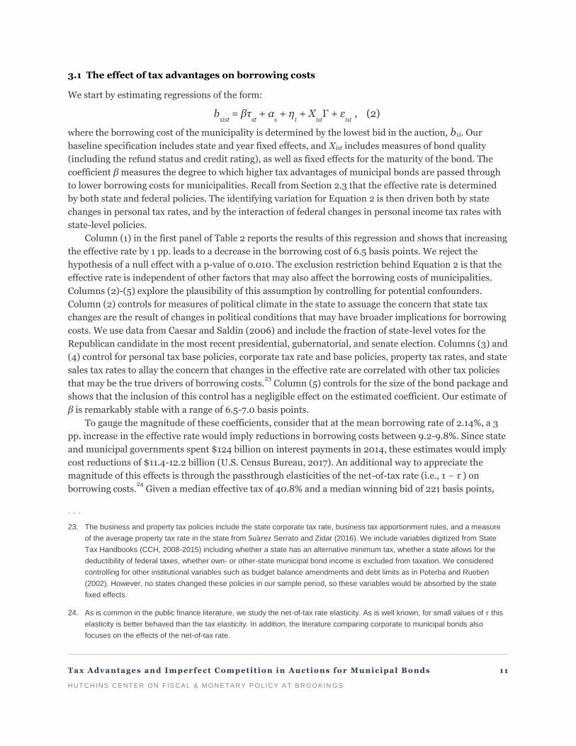
3.1 The effect of tax advantages on borrowing costs
We start by estimating regressions of the form:
b1ist
= βτst
+ αs + η
t + X
istΓ + ε
ist , (2)
where the borrowing cost of the municipality is determined by the lowest bid in the auction, b1i. Our
baseline specification includes state and year fixed effects, and Xist includes measures of bond quality
(including the refund status and credit rating), as well as fixed effects for the maturity of the bond. The
coefficient β measures the degree to which higher tax advantages of municipal bonds are passed through
to lower borrowing costs for municipalities. Recall from Section 2.3 that the effective rate is determined
by both state and federal policies. The identifying variation for Equation 2 is then driven both by state
changes in personal tax rates, and by the interaction of federal changes in personal income tax rates with
state-level policies.
Column (1) in the first panel of Table 2 reports the results of this regression and shows that increasing
the effective rate by 1 pp. leads to a decrease in the borrowing cost of 6.5 basis points. We reject the
hypothesis of a null effect with a p-value of 0.010. The exclusion restriction behind Equation 2 is that the
effective rate is independent of other factors that may also affect the borrowing costs of municipalities.
Columns (2)-(5) explore the plausibility of this assumption by controlling for potential confounders.
Column (2) controls for measures of political climate in the state to assuage the concern that state tax
changes are the result of changes in political conditions that may have broader implications for borrowing
costs. We use data from Caesar and Saldin (2006) and include the fraction of state-level votes for the
Republican candidate in the most recent presidential, gubernatorial, and senate election. Columns (3) and
(4) control for personal tax base policies, corporate tax rate and base policies, property tax rates, and state
sales tax rates to allay the concern that changes in the effective rate are correlated with other tax policies
that may be the true drivers of borrowing costs.23
Column (5) controls for the size of the bond package and
shows that the inclusion of this control has a negligible effect on the estimated coefficient. Our estimate of
β is remarkably stable with a range of 6.5-7.0 basis points.
To gauge the magnitude of these coefficients, consider that at the mean borrowing rate of 2.14%, a 3
pp. increase in the effective rate would imply reductions in borrowing costs between 9.2-9.8%. Since state
and municipal governments spent $124 billion on interest payments in 2014, these estimates would imply
cost reductions of $11.4-12.2 billion (U.S. Census Bureau, 2017). An additional way to appreciate the
magnitude of this effects is through the passthrough elasticities of the net-of-tax rate (i.e., 1 − τ ) on
borrowing costs.24 Given a median effective tax of 40.8% and a median winning bid of 221 basis points,
. . .
23. The business and property tax policies include the state corporate tax rate, business tax apportionment rules, and a measure
of the average property tax rate in the state from Suarez Serrato and Zidar (2016). We include variables digitized from State
Tax Handbooks (CCH, 2008-2015) including whether a state has an alternative minimum tax, whether a state allows for the
deductibility of federal taxes, whether own- or other-state municipal bond income is excluded from taxation. We considered
controlling for other institutional variables such as budget balance amendments and debt limits as in Poterba and Rueben
(2002). However, no states changed these policies in our sample period, so these variables would be absorbed by the state
fixed effects.
24. As is common in the public finance literature, we study the net-of-tax rate elasticity. As is well known, for small values of 𝜏 this
elasticity is better behaved than the tax elasticity. In addition, the literature comparing corporate to municipal bonds also
focuses on the effects of the net-of-tax rate.
_________________________________________________________________________________________________________
Tax Adva ntages an d Im perf ect Competit ion in Auctions for Mu nicipal Bonds 12
HUT C H INS CE NT E R ON F IS C A L & MO N E T A R Y P O L IC Y A T B RO OK IN GS
these estimates imply passthrough elasticities between 1.7-1.9. The estimated elasticities in columns (2)-
(5) reject the hypothesis of a passthrough elasticity below unity at the 10% level.
3.2 The effect of tax advantages on auction participation
We now explore the interaction between tax policy and participation in auctions. First, we estimate an
analogous specification to Equation 2 but where the dependent variable is the number of potential
bidders. The second panel in Table 2 presents the result from this estimation and shows that a higher
effective rate is associated with a larger number of potential bidders. Intuitively, as the value of the bonds
increases with the tax advantage, more bidders are likely to participate in a given auction. The estimates
imply that a 4 pp. increase in the effective rate leads to an increase of close to 2 potential bidders. This is a
large effect as it would move an auction from the median to the 75th percentile of the distribution of
potential bidders. These estimates are also stable across specifications, and Table A.6 shows that a similar
increase is found when using an alternative definition of potential bidders.
As additional potential bidders are likely to lead to lower winning bids, we now explore the degree to
which the results in the first panel are due to tax-driven changes in the competitiveness of a given auction.
The third panel of Table 2 presents estimates of Equation 2 where we now partial out this mechanism by
controlling for fixed effects in the number of potential and actual bidders. Conditioning on auction
competition leads to smaller effects of the tax advantage on borrowing costs, confirming that one of the
mechanisms through which higher taxes lead to lower borrowing costs is through an indirect
competitiveness effect.25 Comparing the results from the first and third panels of Table 2, we find that
between 23% and 31% of the coefficient in the first panel is due to auction competitiveness, which suggest
that the effect of taxes on bidders’ participation decisions are an important determinant of borrowing
costs.26 Finally, we note that removing the indirect effect of taxes on auction competition results in a
smaller passthrough elasticity in the range 1.2-1.4.
3.3 Robustness and causal identification
This section provides evidence that the reduced-form effects from Sections 3.1 and 3.2 are driven by state
tax changes that are plausibly exogenous from other drivers of municipal borrowing costs. We first
discuss how an omitted variable might affect our results. We show that potential confounders, such as
budget or rating shocks, would bias our estimates in the direction of finding a null effect. We then show in
Section 3.3.1 that our estimates are robust to controlling for a battery of potential confounders. Finally, in
Section 3.3.2 we exploit the panel nature of our data to show that the timing of tax changes lines-up with
changes in borrowing costs, and we provide a placebo test that shows that future tax changes are not
predictive of borrowing costs.
. . .
25. Figure A.2 reports the coefficients on the number of bidders fixed effects relative to the median winning bid in the sample,
along with the distribution of this variable. This graph shows that moving from a single bidder to 8 bidders lowers the winning
bid by 30%, on average, but that further increases in the number of bidders do not affect the winning bid. Since a significant
number of bonds have less than 8 bidders, there is substantial scope for lowering municipal borrowing costs by increasing
competition in auctions.
26. We compute standard errors for this quantity by jointly bootstrapping the estimates in the first and third panels and find that,
even in our most demanding specification in Column (5), we can reject the null of no difference with a p-value of 0.084.

_________________________________________________________________________________________________________
Tax Adva ntages an d Im perf ect Competit ion in Auctions for Mu nicipal Bonds 13
HUT C H INS CE NT E R ON F IS C A L & MO N E T A R Y P O L IC Y A T B RO OK IN GS
We begin by considering how an omitted variable could influence the estimates from Equation 2.
While the variation in effective rates comes from the interaction of federal and state tax policy, most of the
variation in the effective rates during our period stems from state tax changes. The exclusion restriction is
then that state tax rate adjustments are uncorrelated from unobserved factors that may also influence
borrowing costs. For example, shocks to local economic conditions, municipal budgets, or the credit-
worthiness of the locality could influence borrowing costs. If one of these factors, labeled Zst, is also
correlated with state tax rates, omitting this factor from the analysis would result in the following bias:
𝑏𝑖𝑎𝑠 = 𝐶𝑜𝑣(𝑍𝑠𝑡 , 𝜏𝑠𝑡)
𝑉𝑎𝑟(𝜏𝑠𝑡)
𝐶𝑜𝑣(𝑍𝑠𝑡 , 𝑏1𝑖𝑠𝑡)
𝑉𝑎𝑟(𝑏1𝑖𝑠𝑡)
Since investors would demand a higher interest rate following a negative economic, budget, or rating
shock, we would expect Cov(Zst, b1ist) > 0, if Zst is one of these events. In order for the omission of Zst to
bias our estimates in any direction, states would need to respond to these shocks by changing tax rates,
i.e. Cov(Zst, τst) ≠ 0. This is an unlikely source of bias since most of the bonds in our dataset are issued by
school districts, cities, and counties who do not set state tax rates, and it is unlikely that states will adjust
state taxes in response to a shock to a local government.
Moreover, the existing literature on how states respond to fiscal pressure shows that states generally
increase taxes when facing state budget shortfalls, so that, if anything, Cov(Zst, τst) > 0. For instance,
Poterba (1994) describes how many states have policies in place that forbid extended periods of deficit
spending, which can force states with unexpected negative fiscal shocks to raise taxes, in which case the
bias would be positive.27
This discussion shows that the most likely potential confounders would bias our
estimates toward zero, and against finding a negative effect of taxes on borrowing rates.
3.3.1 Controlling for potential confounders
Following the discussion in the previous section, we now show that our reduced-form results are robust to
controlling for a battery of potential confounders. Table 3 shows that our estimates are robust to
controlling for local economic conditions, state spending and intergovernmental transfers, and to
including bidder and issuer fixed effects. Columns (2) and (3) use the identity of the winning bidder and
the issuing municipality to test whether unobserved factors at the issuer or buyer levels may confound the
role of effective tax rates. Columns (4) - (7) include additional state economic and spending controls:
unemployment rate, state GDP, government spending, and intergovernmental transfers. Column (8)
includes every control used in the robustness table. In this specification, β is identified by repeated bond
auctions by the same issuer (municipality) with the same bidder (underwriter) in time periods with
different (federal and state) tax rates. This severely limits concerns that our results are driven by omitted
factors that may be correlated with both tax changes and borrowing costs.
The estimated effects of tax rates on the winning bid after controlling for the bidder, issuer, and
economic characteristics are in the range between -6.1 and -7.2, with the lowest and highest estimates
both coming from specifications with issuer fixed effects. These results are remarkably robust across these
. . .
27. Similarly, states are likely to increase tax rates to raise more revenue needed to pay for higher interest rates following a
negative credit-rating shock. We discuss negative shocks for illustration purposes, but a positive shock would also result in a
positive bias since both correlations would be negative in that case.

_________________________________________________________________________________________________________
Tax Adva ntages an d Im perf ect Competit ion in Auctions for Mu nicipal Bonds 14
HUT C H INS CE NT E R ON F IS C A L & MO N E T A R Y P O L IC Y A T B RO OK IN GS
specifications, which suggests that the exclusion restriction is likely to hold. We formalize this evidence of
coefficient stability by using the methods proposed by Altonji et al. (2005) and Oster (2017). Appendix C.5
discusses the results in Table A.9, which suggest that it is extremely unlikely that our main effects are
driven by selection on unobservables. The effect on the number of potential bidders is also stable, with
effects between 0.54 and 0.64 with the additional controls.
We use Table 4 to explore additional potential threats to identification, as well as potential biases due
to variable measurement. One potential concern is that changes in the top marginal tax rate coincide with
market trends in borrowing costs that are not captured by year fixed effects. Columns (2) and (3) of Table
4 expand our baseline specification by including controls for interest rate risk and whether the bond is
callable. Column (2) includes the swap rate between the 3-month and 1-year the London Inter Bank
Offering Rate (LIBOR), which is a strong proxy for bond market uncertainty (Board of Governors of the
Federal Reserve System, 2018), as well as the Securities Industry and Financial Markets Association
(SIFMA) 7-day variable rate demand obligation yield for municipal debt (SIFMA, 2017), which proxies for
market conditions in the municipal bond market. Both of these measures track market conditions at a
high frequency, given that bond market conditions may vary widely within a given year. In Column (2), we
estimate an effect of -6.347, which is very close to our baseline specification from Table 2 included in
Column (1). In addition, in Column (3), we add a dummy variable for whether a bond is callable or not, as
well as fixed effects for the number of years until the first call date. These additional controls result in a
coefficient equal to -6.721, which also lies in the range of the estimates in Table 2.
As discussed in Section 2.3, our measure of effective rates uses the top marginal tax rate in a given
state. This is a reasonable measure since high income individuals are the primary holders of municipal
debt. Moreover, the effects of this variable are of policy interest since the top marginal tax rate is a policy
lever that states can change. However, since the marginal buyer of municipal bonds may not be in the top
income tax bracket, we now show that our results are also robust to using an alternative measure of the
effective tax rate. In Column (4) of Table 4, we re-estimate our baseline model using a measure of the
effective tax rate for the 90th percentile of household income. This specification results in an estimated
effect of -6.394, which is very similar to our baseline estimate.28
3.3.2 Panel data and event study analyses
We now exploit the panel dimension of our data to explore the identifying variation in the effective tax
rate. We start by showing that most of the variation is driven by sub-state agencies that cannot affect the
tax advantage for their bonds. Column (5) of Table 4 reproduces our preferred reduced-form estimates
but excludes all entities that have the ability to change tax rates (states and state agencies) from the
sample. The resulting estimates are nearly identical to those from the regression including entities that
have control over their own tax rates. This result shows that our main estimate is not driven by reverse
causality, where states may change tax rates to influence their borrowing costs. In Appendix C, we provide
. . .
28. Appendix C discusses additional robustness checks. In Table A.5 we show that the standard errors for our estimates are not
overly sensitive to the clustering level. This table also shows that our results are robust to the inclusion of monthly, and even
daily, fixed effects, which assuage concerns that our results are driven by the financial crisis, when large macroeconomic
shocks were happening with greater than annual frequency. Finally, this table shows that our results are not sensitive to
including small bonds, which we exclude from our main specification since they are systematically different from larger bonds
that fund public improvement projects, and since they make up a small fraction of the total value of all issuances.

_________________________________________________________________________________________________________
Tax Adva ntages an d Im perf ect Competit ion in Auctions for Mu nicipal Bonds 15
HUT C H INS CE NT E R ON F IS C A L & MO N E T A R Y P O L IC Y A T B RO OK IN GS
further evidence against the reverse causality hypothesis by showing that state tax rates are unaffected by
previous, current, and future state interest payments.
We now show that changes in state tax rates are an important source of variation in our data. Column
(6) of Table 4 shows that our results are robust to dropping observations from the five states that do not
exempt interest income from state taxation. In column (7) of Table 4 we show estimates of Equation 2
using only variation in state tax rates. For this specification, effective rates are defined according to
Equation 1 except that the federal tax rate is held constant at its 2008 level for all later years. The
estimated coefficient using only state variation in taxes is -5.5, which is not statistically distinguishable
from the preferred estimates. This result gives evidence that the most important identification
assumptions involve state tax changes.
In order to clarify the source of variation, we collapse our data at the issuer-year level and estimate
our main specification in changes over time. This clarifies that our estimates are driven by bond auctions
by the same issuer observed across periods with different tax rates. We take the first difference of
Equation 2 and estimate the regression:
∆b1ist = β∆τ
st + ∆ηt + ∆X
istΓ + ∆ε
ist ,
where the state fixed effect are absorbed in the difference. We restrict the sample of issuers to those with
issues in at least three sets of consecutive years in 2008-2015, which leaves us with 4,692 issuer-year
observations. 48% of the issuer-years in this sample have an associated tax change. We display estimates
of the first differences regression using year fixed effects, quality controls, refund controls, maturity
controls, political controls, other state policy controls, and size controls in panel (a) of Figure 2. The
estimate of β is -9.73 with a standard error of 2.59, which allows us to reject the hypothesis of a null effect
with a p-value of 0.001.
We now show that the timing of the change in borrowing costs lines up with the change in taxes. In
panel (b) of Figure 2 we present a placebo test by replacing ∆τst with ∆τst+1 so that the tax changes happen
in the future. We estimate a placebo coefficient equal to 1.07 with a standard error 2.76 and fail to reject a
null effect in the placebo test with a p-value of 0.701. This shows that municipalities experience a
reduction in borrowing costs immediately after the change in taxes, and that borrowing costs do not
predict tax changes. We provide further evidence that municipalities in states that changed taxes were not
experiencing a secular decline in borrowing costs by estimating an event study of the form:
∆𝑏1𝑖𝑠𝑡 = ∑ 𝛽𝑡−𝑗∆𝜏𝑠𝑡−𝑗 + ∆𝑋𝑖𝑠𝑡Γ
𝑗= −2,1,0,1,2
+ ∆휀𝑖𝑠𝑡.
Figure 3 displays the estimates from this regression using tax changes from 2005-2016 and the average
winning bids at the issuer-year level from 2008-2014. The blue line with circle markers plots the result of
this estimation when we include all of the leads and lags of the tax change variable. This line shows that
there are no significant trends in borrowing costs prior to the tax change, and that the greatest change in
borrowing costs occurs after the tax change. Since the coefficients for the years before the tax change are
not statistically significant (p-value 0.76), we focus on the orange line with diamond markers, which does
not include pre-trends. The estimated effect is stable over time and centers around the coefficient from
our main specification in levels, which equals -6.75 and which is depicted by the green lines with square
markers. While this specification further restricts our data to those municipalities with many bond
_________________________________________________________________________________________________________
Tax Adva ntages an d Im perf ect Competit ion in Auctions for Mu nicipal Bonds 16
HUT C H INS CE NT E R ON F IS C A L & MO N E T A R Y P O L IC Y A T B RO OK IN GS
offerings, it clarifies that the reduced-form effect is identified by municipalities that issue bonds in
periods with different tax rates, and the timing of the changes in tax rates and borrowing costs provides
further evidence that our estimates are not driven by a spurious relation and can be interpreted as causal.
The reduced-form results presented in this section have some immediate implications. First, the
results on borrowing costs suggest that the tax advantage plays a major role in determining
municipalities’ borrowing costs, and that removing the exclusion of municipal bond income from taxation
may significantly affect this market. Second, understanding how tax advantages interact with entry into
auctions is crucial to a full understanding of the passthrough of tax advantages into borrowing costs.
4. Model of participation and bidding in municipal bond auctions
In this section we present a model of participation and bidding in municipal bond auctions. Motivated by
the reduced-form facts in the previous section, the model aims to capture how taxes affect entry into the
auction, how the strategic participation of bidders affects the residual supply for individual bidders, and
how these changes affect the ability of bidders to extract information rents by shading their bids relative
to their valuations. Capturing these margins is important to measure equilibrium markups in each auction
(Section 5), to understand how the effects of taxes on winning bids depends on changes in markups
(Section 6), and in order to analyze counterfactual changes to tax policy (Section 7). Our modeling
approach most closely resembles that of Li and Zheng (2009).29
Consider the auction for a municipal bond by some municipality or state. There are N potential risk-
neutral bidders for this bond offering. The bond will be awarded to the bidder that submits the lowest bid
b. Each bidder i has a private value vi for the bond, which is drawn from a twice continuously
differentiable distribution F (·), with density f (·) that is strictly positive over the support [𝑣, ��]. We
interpret a bidder’s value vi as the net value of selling the bond in the secondary market, which may vary
across bidders due to different bond-buying clientele networks and costs of marketing. To participate in
the auction, each bidder must pay a private entry cost di, which is drawn from a twice continuously
differentiable distribution H(·), with density h(·) that is strictly positive over the support [𝑑, ��]. We
interpret these costs as including the cost of researching the bond for sale, as well as the potential for
resale opportunities in the secondary market, which can reasonably vary across bidders. Section 5
describes how we take this model to the data, where we allow the model primitives to depend on bond
characteristics, including 𝜏. For simplicity, we omit this dependence in the description of the model in this
section.
The informational assumptions of the model are as follows. At the entry stage, each of the N potential
bidders knows his own entry cost di, the number of potential bidders N , and the distributions F (·) and
H(·). If a bidder chooses to participate in the auction by paying di, the bidder learns his value vi, but not
the total number of actual entrants, as bidders in municipal bond auctions do not observe the number of
. . .
29. Appendix D provides additional details behind the model derivation.

_________________________________________________________________________________________________________
Tax Adva ntages an d Im perf ect Competit ion in Auctions for Mu nicipal Bonds 17
HUT C H INS CE NT E R ON F IS C A L & MO N E T A R Y P O L IC Y A T B RO OK IN GS
other competing bidders, which we denote n.30
We assume conditionally independent private values,
similar to other recent work on auctions for financial products (e.g., Hortaçsu et al. (2018)).31
As in Li and Zheng (2009), the model can be altered to incorporate reserve prices, but like them we
will focus on auctions without reserve prices to be consistent with the data. We follow Li and Zheng
(2009) in assuming that each potential bidder holds the belief that if they are the only entrant in the
auction, then the seller will also submit a competing bid based on its own draw from the distribution F (·),
and that if there is more than one entrant, then the seller will not submit a bid. This allows us to
rationalize instances in our data where there is one participating bidder that submits a finite bid. Such an
assumption is necessary since there is no Bayesian-Nash equilibrium bidding strategy with finite bids in
low bid auctions with unknown number of competitors. This is due to the fact that, since there is always a
chance that an entrant faces no competition, there is always an incentive to bid infinity.
4.1 Bidding
We begin with the bidding stage of the model. Upon entry, a participating bidder faces an uncertain
number of competing bidders. The bidder maximizes its expected profits by choosing its optimal bid bi
according to the strictly increasing equilibrium bidding strategy β(·), which depends on the bidder’s
expectation of the number of competitors she will face:
𝐸𝜋(𝑣𝑖|𝑝∗) = ∑𝑷𝑟∗[𝑛 = 𝑘](𝑏𝑖 − 𝑣𝑖) 𝑷r(𝑏𝑖 < 𝑏𝑗 , 𝑗 = 1, … , 𝑛, 𝑗 ≠ 𝑖) + 𝑷𝑟
∗[𝑛 = 1](𝑏𝑖 − 𝑣𝑖) 𝑷𝑟(𝑏𝑖 < 𝑏𝑠) .
𝑁
𝑘=2
Here Pr∗(·) is the equilibrium probability that k bidders participate in the auction, and is given by:
𝑷𝑟∗[𝑛 = 𝑘] = 𝐶𝑁−1𝑘−1(𝑝∗)𝑘−1(1 − 𝑝∗)𝑁−𝑘 , (3)
which depends on an equilibrium entry probability p∗ (defined below), and where 𝐶𝑁−1
𝑘−1 denote binomial
coefficients. In the event that there is only one active participant, i.e. n = 1, we assume that this
. . .
30. Even though bidders in municipal bond auctions do not observe the number of other actual bidders, since the set of firms that
bid in these auctions is relatively stable over time, and typically consists of local branches of large banks, we assume they
know the number of potential entrants, N . Additionally, since 2005, information on every secondary market transaction for
municipal bonds is made available online, and so it is reasonable to assume that auction participants stay at least partially
informed of their competitors’ activities, which is also informative of N , even if, in any particular auction, they don’t know n.
31. When a bank or other broker-dealer wins an auction to be the underwriter of a municipal bond issue, they can hold some of the
debt themselves and sell the rest of the bond package to other institutional and individual investors. The bidder’s value
depends on their own demand for the bond, and on the demand of the clientele with whom they deal. The networks through
which different underwriters place bonds vary geographically and along other margins. For instance, Babina et al. (2015) show
that tax exemptions for municipal debt create ownership segmentation by state because the interest is exempt in the issuing
state and not other states. Similarly, Green et al. (2007) present evidence that individual investors have differing levels of
information, so that different investors pay different prices for the same bond. Green et al. (2007) also present an overview of
the process by which municipal bonds reach the secondary market and why underwriters may have idiosyncratic
considerations. Given that banks do not have identical clienteles geographically or otherwise, their values would not be
changed by knowing the values of other potential bidders in a given auction. Tang (2011) and Shneyerov (2006) use a set of
municipal bond auctions from before the start of our sample to analyze questions of mechanism design without imposing
informational assumptions on the bidders. Interestingly, Tang (2011) shows that making incorrect assumptions about bidder
values has negligible impacts on expected revenue.
_________________________________________________________________________________________________________
Tax Adva ntages an d Im perf ect Competit ion in Auctions for Mu nicipal Bonds 18
HUT C H INS CE NT E R ON F IS C A L & MO N E T A R Y P O L IC Y A T B RO OK IN GS
participant competes against the seller. In the equation for profits above, bid bs represents a virtual bid by
the seller, and it is assumed to have the same distribution as the bid of a randomly chosen participant.
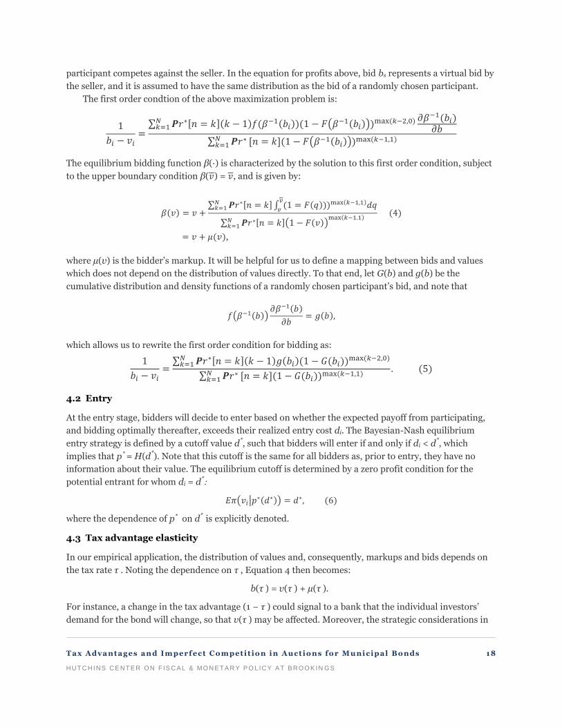
The first order condtion of the above maximization problem is:
1
𝑏𝑖 − 𝑣𝑖=∑ 𝑷𝑟∗[𝑛 = 𝑘](𝑘 − 1)𝑓(𝛽−1(𝑏𝑖))(1 − 𝐹(𝛽
−1(𝑏𝑖)))max (𝑘−2,0) 𝜕𝛽
−1(𝑏𝑖)𝜕𝑏
𝑁𝑘=1
∑ 𝑷𝑟∗𝑁𝑘=1 [𝑛 = 𝑘](1 − 𝐹(𝛽−1(𝑏𝑖)))
max(𝑘−1,1)
The equilibrium bidding function β(·) is characterized by the solution to this first order condition, subject
to the upper boundary condition β(𝑣) = 𝑣, and is given by:
𝛽(𝑣) = 𝑣 +∑ 𝑷𝑟∗[𝑛 = 𝑘] ∫ (1 = 𝐹(𝑞)))max(𝑘−1,1)𝑑𝑞
𝑣
𝑣𝑁𝑘=1
∑ 𝑷𝑟∗[𝑛 = 𝑘](1 − 𝐹(𝑣))max(𝑘−1.1)𝑁
𝑘=1
(4)
= 𝑣 + 𝜇(𝑣),
where µ(v) is the bidder’s markup. It will be helpful for us to define a mapping between bids and values
which does not depend on the distribution of values directly. To that end, let G(b) and g(b) be the
cumulative distribution and density functions of a randomly chosen participant’s bid, and note that
𝑓(𝛽−1(𝑏))𝜕𝛽−1(𝑏)
𝜕𝑏= 𝑔(𝑏),
which allows us to rewrite the first order condition for bidding as:
1
𝑏𝑖 − 𝑣𝑖=∑ 𝑷𝑟∗[𝑛 = 𝑘](𝑘 − 1)𝑔(𝑏𝑖)(1 − 𝐺(𝑏𝑖))
max (𝑘−2,0)𝑁𝑘=1
∑ 𝑷𝑟∗𝑁𝑘=1 [𝑛 = 𝑘](1 − 𝐺(𝑏𝑖))
max(𝑘−1,1). (5)
4.2 Entry
At the entry stage, bidders will decide to enter based on whether the expected payoff from participating,
and bidding optimally thereafter, exceeds their realized entry cost di. The Bayesian-Nash equilibrium
entry strategy is defined by a cutoff value d∗, such that bidders will enter if and only if di < d
∗, which
implies that p∗ = H(d
∗). Note that this cutoff is the same for all bidders as, prior to entry, they have no
information about their value. The equilibrium cutoff is determined by a zero profit condition for the
potential entrant for whom di = d∗:
𝐸𝜋(𝑣𝑖|𝑝∗(𝑑∗)) = 𝑑∗, (6)
where the dependence of p∗ on d
∗ is explicitly denoted.
4.3 Tax advantage elasticity
In our empirical application, the distribution of values and, consequently, markups and bids depends on
the tax rate τ . Noting the dependence on τ , Equation 4 then becomes:
b(τ ) = v(τ ) + µ(τ ).
For instance, a change in the tax advantage (1 − τ ) could signal to a bank that the individual investors’
demand for the bond will change, so that v(τ ) may be affected. Moreover, the strategic considerations in
_________________________________________________________________________________________________________
Tax Adva ntages an d Im perf ect Competit ion in Auctions for Mu nicipal Bonds 19
HUT C H INS CE NT E R ON F IS C A L & MO N E T A R Y P O L IC Y A T B RO OK IN GS
the optimal bidding function and zero profit conditions (Equations 4 and 6) may also impact equilibrium
information rents, leading to a change in µ(τ ).
The expression above provides a simple way to decompose the elasticity of a bidder’s bid with respect
to the tax advantage, 1 − τ :
𝜕𝑏
𝜕(1 − 𝜏)
(1 − 𝜏)
𝑏=
𝜕𝑣
𝜕(1 − 𝜏)
(1 − 𝜏)
𝑏+
𝜕𝜇
𝜕(1 − 𝜏)
(1 − 𝜏)
𝑏
or,
휀1−𝜏𝑏 = (1 −𝑚)휀1−𝜏
𝑣 +𝑚휀1−𝜏𝜇, (7)
where m is the markup rate µ/b, and ε are elasticities of the model variables in 1 − τ . This expression
allows us to relate the model to the reduced-form results in Section 3, and to decompose the tax
advantage elasticity of bids into the effects on values and markups, which we do in Section 6.
5. Structural estimation and implied markups
We now outline the estimation of the model, discuss estimation results, and describe the estimated
equilibrium markups. To take the model to the data, we allow for bidders’ bond valuations to depend on
bond-specific characteristics that may or may not be observable to the econometrician. Consider an
auction for municipal bond j with characteristics Xj and Zj , which are observable to the econometrician as
well as the bidders. Bidder i’s value for this bond is given by vij = ��𝑖𝑗+ uj , where uj represents
heterogeneity across bonds that is observable to the bidders but not the econometrician, and ��𝑖𝑗 are i.i.d.
for each bidder i.32
The additive structure of the bidders’ idiosyncratic values for bond j and the
unobservable heterogeneity component imply that bidder i’s bid bij = ��𝑖𝑗+ uj , where ��𝑖𝑗 can be interpreted
as the bidder-specific bid component. At the entry stage, each of the Nj potential bidders observe Xj and uj
, realize their idiosyncratic private information entry costs dij , and decide whether to enter based on their
expected profits from participating in the auction.
5.1 Estimation
We estimate this empirical model using a two-step estimation approach. In the first step we estimate
parameters of the bid (𝜃��), entry cost (θd), and unobservable heterogeneity distributions (θU ), and in the
second step we back out the distribution of bidder values following the arguments of Guerre et al.
(2000).33
We parametrize the model as follows:
. . .
32. As is standard (e.g., Krasnokutskaya and Seim (2011)), we assume that uj is independent of Xj and the number of potential
bidders Nj . However, as we will assume that both Xj and uj will be observable to bidders before they take their entry decisions,
it need not be independent of the actual number of entrants, nj .
33. A similar approach is used elsewhere in the literature (e.g., Krasnokutskaya and Seim (2011) and Athey et al. (2011)).
Compared to the alternative approach of parameterizing the values, this method enables us to lessen the computational
burden of the estimation procedure and include a richer set of controls.

_________________________________________________________________________________________________________
Tax Adva ntages an d Im perf ect Competit ion in Auctions for Mu nicipal Bonds 20
HUT C H INS CE NT E R ON F IS C A L & MO N E T A R Y P O L IC Y A T B RO OK IN GS
Bid Distribution: 𝑔(𝑏; 𝜃��) =N(𝑋𝑗𝛽, 𝑒𝑋𝑗𝛾, 𝑋𝑗𝛿,∞)
Entry Cost Distribution: ℎ(𝑑𝑗; 𝜃𝑑) = 𝑙𝑛N(𝑘1, 𝑘2)
Unobservable Heterogeneity Distribution: 𝑓𝑈(𝑢; 𝜃𝑈) =N(𝑍𝑗𝛤, 𝜎𝑈)
where N (µ, σ, a, b) is a truncated Normal distribution with mean µ, standard deviation σ, lower
truncation point a and upper truncation point b,34
𝑙𝑛N (c, d) is a Log-Normal distribution with location
parameter c and scale parameter d, and N (e, f ) is a normal distribution with mean e and standard
deviation f .35
We estimate the model using maximum likelihood. For a candidate θ = {𝜃��, θd, θU }, the likelihood of
observing the set of entry and bidding decisions in auction j is:
L(𝜃) = ∏ 𝐶𝑁𝑗𝑛𝑗��𝑗(𝜃)
𝑛𝑗 (1 − ��𝑗(𝜃))𝑁𝑗−𝑛𝑗
𝑔 (𝑏1, … , 𝑏𝑛𝑗; 𝜃), (8)𝐽𝑗=1
where 𝑔 (𝑏1, … , 𝑏𝑛𝑗; 𝜃) is the joint density of bids in auction j, and ��𝑗(𝜃) the equilibrium entry probability
associated with parameters θ. We compute these entry probabilities as follows. First, following Equation
5, define the expected profits of submitting bid �� for any given probability of entry p as
𝐸𝜋(��|𝑝) =1
𝑔(��; 𝜃��)∑ [𝑷𝑟∗[𝑛 = 𝑘] (1 − 𝐺(��; 𝜃��))
max(𝑘−1,1)
] ,
𝑁
𝑘=1
with Pr∗ [n = k] defined in Equation 3. The entry probability ��𝑗 is given by the probability that the entry
cost 𝑑𝑖𝑗 is below the entry cost implied by the zero profit condition in Equation 6.36
After maximizing
Equation 8 to recover estimates ��, we recover the implied value 𝑣𝑖𝑗 corresponding to each bid bij using
Equation 5.
. . .
34. Note that the observables in our model are b rather than ��, and their distribution is not truncated. Consequently, the standard
MLE asymptotic results are valid for our parameter estimates. In practice, the variance of bids is typically low enough that Xβ −
��, where �� is the lower truncation point of bids, is so large that having or not having the lower truncation threshold has virtually
no impact on simulated bids. However, it is important to have truncation to ensure existence of equilibrium in the model.
Furthermore, the model itself predicts that, given some distribution of values, bids in equilibrium will naturally have some lower
cutoff level.
35. We model the unobservable heterogeneity as having unconstrained support, which is convenient for MLE. While this choice
does allow the possibility for negative bids, our estimates suggest that this is very unlikely (with about a 0.02 probability that the
winning bid is negative across our sample). For this reason, we are comfortable with this parameterization, since it is unlikely
that truncating fU (·) would materially impact our results.
36. To determine the unique solution to Equation 6 we evaluate the left-hand-side of the zero profit condition with
𝐸𝜋(𝑝∗) = ∫ 𝐸𝜋(��|𝑝∗, 𝑢 = 0)𝑔(��; 𝜃��)𝑑��∞
��.
Note here that we leverage the fact that bids and values are linear functions of the unobservable, which imply that bidder’s
profits are independent of u, and it is enough to compute them just for u = 0. This is in contrast to Athey et al. (2011), where
profits of bidders are proportional to a function of unobservable u, and Krasnokutskaya and Seim (2011), where profits are
proportional to u.

_________________________________________________________________________________________________________
Tax Adva ntages an d Im perf ect Competit ion in Auctions for Mu nicipal Bonds 21
HUT C H INS CE NT E R ON F IS C A L & MO N E T A R Y P O L IC Y A T B RO OK IN GS
We note that our model is nested within the framework of Gentry and Li (2014), who study
nonparametric identification in auction models where potential bidders can observe a noisy, and
potentially independent, signal of their value prior to entry. They show that with sufficient exogenous
variation in signal thresholds, which could stem from variation in the number of potential bidders, the
model is non-parametrically point identified even in the presence of unobserved auction-level
heterogeneity. In order to credibly study the impact of the effective rate and other policy tools (like the
excludability of interest income from state taxation) on the issuer’s total borrowing costs, we adopt a
parametric estimation approach, which allows us to include an extensive set of covariates in the model.
5.2 Estimation results
The baseline model parametrizes the mean of the distribution of bids as a linear function of the number of
potential bidders, the maturity of the bond, and the effective rate. For unobservables, we allow for the
mean of the distribution to have different values for every state and every year. The mean of the
distribution is also allowed to vary linearly with a number of the controls used in Section 3.37 The standard
deviation is parameterized as the exponential of a linear function of the number of potential bidders, the
maturity of the bond, and the effective rate. The lower threshold of the distribution of bids is parametrized
as a linear function of the same observables.
Estimation results for the baseline model are reported in Table 5. The estimate for the effect of τ on
the mean of the parametrized distribution of bids, ��, has a similar sign and magnitude as in the reduced-
form estimates of Table 2 that condition on entry: a 1 pp. increase in τ leads to a 4.2 basis point decrease
in bids, on average.38 We also find that τ has a negative effect on the standard deviation of the
parametrized distribution of bids, 𝛾. This implies that the dispersion in bids decreases as the tax
advantage increases, which may affect equilibrium markups.
The estimated model fits the data well. Figure 4 shows that the model fits the entire distribution of
winner’s bids across the sample.39 We also match entry rates, n/N , well. For example, the average
(median) probability of entry in the data is 0.701 (0.714), and our model predicts it to be 0.728 (0.728).
We use the model estimates to simulate entry costs and bidder markups. We find that the median
threshold entry cost in our data d∗ is 0.35%. At the median bond size offering, this translates to an entry
cost of about $35,000, which may be reasonably commensurate with the costs of engaging in pre-sale
marketing activities, as well as performing due diligence on the particular bond offering. Table 6 presents
our model’s estimates of bidder markups. The first row in Table 6 shows that markups are 16.8 basis
. . .
37. These include sales, corporate, and property tax rates, political party measurements for senate, president, and governor
support, and, finally, major party index. Note that we exclude auctions in the state of Nebraska (18 auctions) from the
estimation due to missing data. Table A.4 confirms that our reduced-form results are robust to using this set of controls.
38. Since 𝜏 affects the lower threshold for the distribution of bids, the effect on the distribution mean may not directly reflect the
effect from a shift in 𝜏 on the average bid. However, we find that the threshold is sufficiently far from the mean for typical values
of observables in the data, which reduces the concern of this bias.
39. The bi-modal distribution of winning bids evident in the figure stems from differing maturities, with the first “hump” being largely
associated with maturities equal to one year. Thus, including maturities in our model proves crucial to matching these patterns
in the data.

_________________________________________________________________________________________________________
Tax Adva ntages an d Im perf ect Competit ion in Auctions for Mu nicipal Bonds 22
HUT C H INS CE NT E R ON F IS C A L & MO N E T A R Y P O L IC Y A T B RO OK IN GS
points, on average. Relative to the winning bid, m1/b1, the average markup rate is 17.4%. Table 6 also
reports the dollar value of the markup over the life of the bond, m1st, with an average value of $173,476.40
Our model predicts rich patterns of heterogeneity in markups. The remaining rows in Table 6 show
that auctions for state bonds result in smaller markups, both in levels and as a percent of borrowing costs.
However, since state bonds are larger and have longer durations, the dollar value over the life of the bond
is greater than average. We also find that bonds for school districts and smaller jurisdictions, such as
cities and counties, have significantly larger markups. In particular, bonds issued by local governments
are hurt in part by less participation. On average, about five bidders submit bids for bonds issued by
cities, towns, and villages, whereas more than eight typically submit bids for bonds issued by states. This
suggests that there is substantial scope for lowering municipalities’ borrowing costs by targeting auctions
with high markup rates, or with low participation.41
Figure 5 shows how markups vary with the effective rate and the number of potential bidders. As
expected, we find larger markups in auctions with low numbers of potential bidders, and we find that
markups decrease fairly rapidly in the number of potential bidders. We also find markups are larger when
the tax advantage is smaller, and that this pattern is most pronounced in auctions with low numbers of
potential bidders, which is consistent with the results across issuer types discussed above.
We illustrate the robustness of our results to alternative models that allow for different
parameterizations, flexible effects of covariates, and different definitions of potential bidders. Appendix E
discusses these models, and Table A.12 shows that we obtain good model fit, and similar estimated
markups, across these alternative specifications.
6. Tax incidence in auctions
In this section we explore in more depth the mechanisms by which the tax exemption for municipal debt
affects bidder behavior, and consequently, borrowing costs. Our analysis characterizes the within-auction
incidence assuming that the supply of bonds is not affected by changes in tax advantages. In the
appendices we provide empirical support for this assumption, which is also in line with other findings in
the literature, as well as the institutional features of this market.42
Equation 7 shows the basic intuition
behind the effects that tax rates have the borrowing costs. First, if there is perfect competition, m = 0 and
. . .
40. The markups we find are in line with estimates of ex-post surplus for winners calculated in Hortaçsu et al. (2018) in treasury
auctions. They estimate surpluses between 0.7 and 22 basis points for primary dealers on maturities ranging from 52 weeks to
10 years.
41. In ongoing work (Garrett et al., 2018), we are exploring in greater detail the heterogeneity across auctions, and dynamics over
time, of markups in municipal bond auctions.
42. For instance, Adelino et al. (2017) find that municipalities do not react to rating changes by borrowing more often, and Gordon
and Metcalf (1991) discuss that municipalities do not invest more with lower interest rates caused by the tax exemption in part
due to caps on tax-exempt borrowing. This assumption is consistent with the institutional setting, since many of these bonds
are authorized by popular referenda or by public budgeting processes that limit municipalities’ ability to respond by changing
the size of the issuance or by issuing additional bonds. We provide empirical evidence for this assumption by showing in
column (5) of Table 2 that controlling for the size of the issuance does not affect our reduced-form results, and by showing in
Appendix C.3 that there is not a meaningful response in the supply of issuances to changes in 𝜏 .

_________________________________________________________________________________________________________
Tax Adva ntages an d Im perf ect Competit ion in Auctions for Mu nicipal Bonds 23
HUT C H INS CE NT E R ON F IS C A L & MO N E T A R Y P O L IC Y A T B RO OK IN GS
휀1−𝜏𝑏 = 휀1−𝜏
𝑣 . Second, when m > 0, 휀1−𝜏𝑏 may be greater than or less than one depending on the effect of
changing taxes on markups and bidder values. For example, if 휀1−𝜏𝑣 = 1 then if 휀1−𝜏
𝑏 > 1, it must be the
case that 휀1−𝜏𝜇
> 1.43
This points to the central role played by the responsiveness of markups to changes in
taxes in determining how taxes pass through to borrowing costs.
The following example, shown in Table 7, decomposes this passthrough using our model and a
representative auction from our data. Consider an auction with six potential bidders, τ = 0.35, other
observables set to their median realizations, and a bidder whose value is such that, according to our
estimated model, he would submit a bid equal to the median bid in our data for auctions with these
characteristics. At the original tax rate, the bidder has a value of 1.621 and an optimal bid of 1.896, which
implies a markup rate of 15%. If τ increases from 0.35 to 0.39, his bid will change for a variety of reasons.
First, his value will change, which will lead him to submit a lower bid, even when holding constant his
probability of winning and the number of potential entrants in the auction. This is illustrated in the
second row of the table, which shows that the optimal bid decreases from 1.90 to 1.83 (휀1−𝜏𝑏 = 0.567), when
the value drops from 1.62 to 1.52 (휀1−𝜏𝑣 = 1.002). Second, because other bidders’ values change, the
bidder’s probability of winning changes, which forces him to further lower his bid. This is shown in the
third row of the table, where we adjust the probability of winning to reflect the model estimated winning
probability at the new tax rate and original number of potential bidders. The optimal bid falls to 1.76,
which implies a bid elasticity of 1.16. Finally, the four percentage point effective tax rate increase is
associated with two more underwriters joining the pool of potential bidders (see Table 2). The increase in
competition for the bond, captured by our further adjustment of the probability of winning to reflect the
model estimated winning probability at the new tax rate and the new number of potential bidders, further
depresses the bidder’s bid to 1.69, for a bid elasticity of 1.75. The importance of markups for generating
greater-than-one passthrough of taxes to bids is evident in the final column of the table. In row three,
when all but the effect of τ on N is allowed for, 휀1−𝜏𝜇
= 2.07. Once N is allowed to increase in τ , 휀1−𝜏𝜇
= 6.15.
This example is representative of the rest of our data, in which the average markup rate is 17%
(compared to 15% in the example). According to our model estimates, the average elasticity of bid with
respect to take-home rate in the sample is 2.09, which is comparable to the bid elasticity shown in row
four of Table 7 equal to 1.75, and to our reduced-form estimates in Table 2. The average elasticity of
markups with respect to take-home rate in our sample is 4.93, which also closely mirrors the example’s
value of 6.15.
The example in Table 7 also illustrates that as the tax rate increases, bidder markups decrease, from
0.28 in row one, to 0.17 in row four, and it is the large decline in these markups that leads to greater-than-
one pass through to borrowing rates. We now explore how taxes impact markups and provide non-
parametric evidence that these mechanisms are at play in the data. As made clear in Equation 4, a bidder
trades off the benefit of increasing their bid and enjoying a greater markup over their value in the event
they win the auction, against the possibility that they lose the auction with this higher bid. In particular,
denoting the dependence of values, and thus the probability of winning an auction, on the tax rate,
. . .
43. The case of 휀1−𝜏𝑣 = 1 can occur if one assumes that 𝑣 = ��(1 − 𝜏), where �� is the pre-tax value of a bond. However, we do not
impose this restriction in our model.

_________________________________________________________________________________________________________
Tax Adva ntages an d Im perf ect Competit ion in Auctions for Mu nicipal Bonds 24
HUT C H INS CE NT E R ON F IS C A L & MO N E T A R Y P O L IC Y A T B RO OK IN GS
𝑏 = 𝑣 +𝐏r (𝑣; 𝜏)
−𝜕𝜕𝑏𝐏 r(𝑣; 𝜏)⏟
Markup
where Pr(v; 𝜏 ) is the equilibrium probability of winning the auction when a bidder’s value is v and the tax
rate is 𝜏 . The markup, or difference between a bidder’s bid and the value, depends on the expected market
share, given by Pr and the slope of the inverse supply, given by −𝜕
𝜕𝑏𝐏r. In a perfectly competitive auction,
characterized by many bidders, or by a lack of heterogeneity in bidder valuations, the expected market
share for a given bidder that bids above her valuation is zero, and the inverse supply is vertical at this
valuation. These forces eliminate the possibility for markups. As in monopsonistic settings, bidders in
auctions with imperfect competition may “shade” their bids to manipulate the expected market share.44
The fundamental expression of market power in this case is the ability of bidders to improve their
expected surplus by shading their bid, which is controlled by the slope of the inverse supply.
Therefore, the question of how taxes affect markups, and consequently the cost of borrowing via
Equation 7, hinges on how taxes affect the probability associated with a bidder winning an auction at any
particular submitted bid. Specifically, the elasticity of markups with respect to taxes can be decomposed
as follows:
휀1−𝜏𝜇
= 휀1−𝜏𝐏r⏟
change in own market share + 휀1−𝜏
−1/𝜕
𝜕𝑏𝐏𝐫
⏟
change in inverse supply slope
. (9)
An increase in the tax advantage may decrease the markups (and borrowing rates) by decreasing the
market share for a given bidder, and by increasing the slope of the inverse supply. Intuitively, if greater
tax advantages increase the number of actual bidders, the expected market share will decrease. To
interpret 휀1−𝜏−1/
𝜕
𝜕𝑏𝐏r
consider that the slope in the inverse supply is driven by heterogeneity in the
valuations for bonds. If larger tax advantages lead to a selection of bidders with less heterogeneous
valuations for the bond, this will lead to a positive value of 휀1−𝜏−1/
𝜕
𝜕𝑏𝐏𝐫
. This is consistent with results from
Babina et al. (2015), who show that there is a higher degree of tax-induced ownership segmentation in
states with a larger tax advantage for municipal bonds. Intuitively, since only residents of the issuing state
receive the full tax benefit, as the state tax rate increases, it is more likely that residents of the state own
the bonds, and that the distribution of their valuations is more compressed. This is also consistent with
. . .
44. We use the phrase “shade” as it is common in the literature on first-price auctions, even though in this low-bid setting, the
bidders seek to inflate their bid above their value.

_________________________________________________________________________________________________________
Tax Adva ntages an d Im perf ect Competit ion in Auctions for Mu nicipal Bonds 25
HUT C H INS CE NT E R ON F IS C A L & MO N E T A R Y P O L IC Y A T B RO OK IN GS
our structural estimates in Section 5.2, where we find that an increase in τ is associated with a smaller
variance of the distribution of bids.
While the model imposes parametric structure in order to incorporate a rich set of observables, we
now show that the key interactions between taxes and the probability of winning an auction are evident in
the raw data. Specifically, we show how changes in τ affect non-parametric estimates of the probability of
winning. We begin by estimating the probability of winning an auction using the kernel estimator:
𝐏r [𝑏−i > 𝑏|𝑁, 𝑋] =∑1𝑛𝟏(𝑏𝑗 > 𝑏)𝐾 (
𝑋𝑗 − 𝑋ℎ𝑋
)𝑗
∑ 𝐾 (𝑋𝑗 − 𝑋ℎ𝑋
)𝑗
,
where j is an indicator for each auction, and 𝟏(𝑏𝑗 > 𝑏)is an indicator that b is below all bids in auction j.
K(·) is a kernel that assigns weights to the auctions based on observable characteristics Xj . We use
triweight kernels with bandwidth ℎ𝑋 = c · std(X) · (J )−1/5
, where J denotes the number of auctions, std(X)
measures the standard deviation of X, and c ≈ 3 is the kernel-specific constant. We condition on the
number of potential bidders N , on the effective tax rate τ , and on maturity between 2 and 17 years, which
corresponds to the middle tercile of the length distribution.
Figure 6 plots this estimated probability for different values of N and τ . The fundamental expression
of market power in our setting is the ability of bidders to trade-off higher surplus for a smaller expected
market share. The data reveal whether bidders may profit from such strategic bidding by showing that the
probability of winning has a finite slope around the winning bid. The blue solid lines correspond to
estimated probabilities of winning for the mean value of τ = 0.35 and for N = 4, 6, 8, 10. These lines show
that auctions for municipal bonds are far from the ideal of perfect competition as the finite slope allows
for bidders to strategically shade their bids. As one would expect, the probability of winning has a steeper
slope when bonds have a larger number of potential bidders.
The green dotted and red dashed lines in Figure 6 show that the intuition from the example in Table 7
is apparent in the raw bidding data. For each value of N , the red dashed line plots the estimated
probability of winning with a higher τ = 0.39. These plots show that auctions with larger tax advantages
reduce the scope for markups since both the probability of winning decreases, and the slope of this
probability becomes steeper along most of its domain. As discussed above, higher effective rates also lead
to increases in N . In particular, a reform that increases τ from 0.35 to 0.39 would also lead the average N
to increase by about two additional potential bidders. The green dotted lines plot the probability of
winning with a higher rate and the accompanying increase in N . Highlighting the intuition from the
representative bidder above, these graphs show that the scope for markups is further reduced by the
indirect effect of the tax advantage on the level of competition.
The results from this section highlight the value of measuring markups with our auction model, as
this allows us to show that the effect of the tax advantage on the winning bids is driven by a large effect on
equilibrium markups. Moreover, this mechanism is not dependent on the parametric structure we use in
estimation, as the non-parametric estimates of the probability of winning show that the interaction
between taxes and imperfect competition is visible in the raw data. The following section further

_________________________________________________________________________________________________________
Tax Adva ntages an d Im perf ect Competit ion in Auctions for Mu nicipal Bonds 26
HUT C H INS CE NT E R ON F IS C A L & MO N E T A R Y P O L IC Y A T B RO OK IN GS
highlights the benefits of our structural model, as we use it to simulate the effects of counterfactual
policies on municipal bond auctions.
7. Counterfactual policy analysis
The tax advantages enjoyed by municipal bonds are the subject of intense debate. Several federal reforms
have been proposed that directly or indirectly deal with the growing tax expenditure of the exemption of
municipal interest. We provide a survey of proposed reforms in Appendix F. In this section, we evaluate
reforms that modify the tax advantage by changing the effective rate used in our analysis. Three examples
of reforms include repeated proposals by the Obama administration to limit the exemption to 28%, the
Tax Cut and Jobs Act of 2017 (TCJA17) which lowers the top federal rate to 37% and limits the deduction
for state and local taxes (SALT), as well as other proposals that completely eliminate the exemption. We
fit these three reforms into a general approach that evaluates the consequences of a change in federal tax
rates, by parametrizing the effective tax rate as follows:45
𝜏(𝛼𝑡𝑓 , 𝑡𝑠) = 𝛼𝑡𝑓(1 − 𝑡𝑠) + 𝑡𝑠 × 𝟏(𝑇𝑎𝑥 𝐸𝑥𝑒𝑚𝑝𝑡)𝑆𝑡𝑎𝑡𝑒 .
Relative to the average federal rate from 2011 to 2015, eliminating the federal exemption corresponds to 𝛼
= 0; the Obama proposal corresponds to 𝛼 = 0.73 ≈ 0.28/0.386; and the TCJA17 sets 𝛼 = 0.96 ≈
0.37/0.386. We can also consider the effect of a super exemption of municipal bond interest by evaluating
reforms that set 𝛼 > 1. Additionally, we use the model to evaluate the impact of other policies such as
removing the state exemption of municipal bond interest income from state taxation (for those states that
currently allow it), and to consider the elimination of the deduction for state and local taxes (SALT).
Finally, we study the total effect of the TCJA17, as the decrease in marginal rates and limiting of SALT
affect borrowing costs in opposite directions.
We begin by focusing on changes to the federal tax code that limit or expand the exemption of
municipal bond interest income from federal taxation. For the purposes of this section, we vary α and
simulate auction outcomes for two different cases: when shifts in τ are assumed to have no impact on N ,
and when they are assumed to affect N . We simulate the effect of this policy change on every auction from
2013 to 2015 and present the average of the simulated effects in Figure 7. In this graph, values of 𝛼 < 1
correspond to decreases in the tax advantage, while values of 𝛼 > 1 increase the tax advantage through
increases in the tax rate, or through a form of super exemption. As the tax advantage is decreased from 𝛼
= 1, we see an increase in both the winning bids and the markups, with larger effects corresponding to the
full reform that allows for changes in N . While the effects on the winning bid are close to being linear in
𝛼, the full effects on markups (dashed green line) are strongly concave in 𝛼.
Table 8 presents average effects of specific policies. Recall that the proposal of the Obama
administration is equivalent to reducing α to 0.73. The total effect of this reform would increase the
average borrowing cost by 30.6%, which would imply an additional $38 billion in interest payments by
state and local governments. Without further behavioral responses, the reduction in the tax expenditure
. . .
45. This formula is exact whenever states do not allow for the deductibility of federal taxes from state taxes. We modify the formula
accordingly for the few states that allow this deduction. Note that state taxes are always deducted from federal taxation.

_________________________________________________________________________________________________________
Tax Adva ntages an d Im perf ect Competit ion in Auctions for Mu nicipal Bonds 27
HUT C H INS CE NT E R ON F IS C A L & MO N E T A R Y P O L IC Y A T B RO OK IN GS
over the next decade would be close to $135 billion (≈ (1 − 0.73) × $500 billion). On a yearly basis, this
subsidy represents a gain of $2.8 (≈38
13.5) in state and local funds for every dollar of federal funds. This
subsidy would thus improve welfare as long as the marginal cost of public funds for the federal
government is not 2.8-times greater than the marginal value of providing public goods from municipal
bonds.46
We now explore how these proposals would affect different states. Figure 8 plots the effects of setting
α = 0.73. Panel (a) plots the observed average winning bids by state, and Panel (b) presents the simulated
average winning bid by state after capping the excludability, but without allowing for the additional
potential entry. The effects vary across states depending on a number of factors.47
First, since state taxes
are deducted from federal taxes, changes in federal taxes have larger effects in states with low or no state
income taxes. Indeed, we see large increases in states like Texas, Florida, Nevada, and Wyoming. Second,
the effects of this reform would depend on the distribution of bond characteristics across states, such as
the average length of the bond. Panel (c) simulates the effects of the reform allowing for the effect of the
reform on potential entry. Overall, we see larger increases in borrowing costs. In particular, states that
have few potential bidders may be most affected by this channel. Panel (d) shows that the increase in
winning bids ranges from 48-68 basis points. States with borrowing cost increases greater than 60 basis
points include Texas, New York, New Jersey, Michigan, and Georgia. Figure 9 performs a similar analysis
for the markups across states. While average markups are about 17 basis points, the reform leads to
substantial increases, particularly due to the entry margin.
We perform three additional tax policy analyses. First, we consider the effects of completely
eliminating the excludability of municipal bond interest income at the federal level; that is, setting α = 0.
While this policy represents a level of variation that is outside of our sample, our model implies that
moving to a full repeal of the exemption would result in significantly larger borrowing rates with an
average of 3.64%, of= which 43% (≈ 1.58%
3.64%) would correspond to markups. Figures A.6-A.7 showcase the
large and heterogeneous effects from this policy. Second, Figures A.8-A.9 simulate the effects of
eliminating the state exemption. While eliminating the state exemption leads to an increase in the
. . .
46. This calculation assumes that the increase in borrowing costs does not also increase the federal tax expenditure and ignores
the externality on state governments who would also see an increased tax expenditure. Further, the federal government is not
likely to recoup the full reduction in the tax expenditure because of behavioral substitution away from municipal bonds to other
investment instruments described by Poterba and Verdugo (2011), so $135 million is an upper bound on the revenue cost of
the tax expenditure. These forces imply that the efficiency ratio of 2.8 is a lower bound. We also assume the total value of
issuances to be fixed, which is in line with the existing the results from this and other papers. This is also a conservative
calculation relative to a linear extrapolation of the results of Table 2, where the implied decrease in 𝜏 for α = 0.73 of 33.39% −
43.76% = −10.37% would imply a percentage decrease in borrowing costs of 35.40% (≈10.37%×6.53
1.91) and imply a ratio of 3.25
(≈35.40%×124
13.5).
47. Note that Montana and Nebraska have no auctions from 2013 to 2015 and are excluded from the simulations.

_________________________________________________________________________________________________________
Tax Adva ntages an d Im perf ect Competit ion in Auctions for Mu nicipal Bonds 28
HUT C H INS CE NT E R ON F IS C A L & MO N E T A R Y P O L IC Y A T B RO OK IN GS
importance of the federal subsidy, this potential reform results in an overall decrease in the subsidy. As
expected, we find that states with higher taxes would see larger increases in borrowing costs. As shown in
Table 8, average borrowing costs would rise nearly 16%, and markups would nearly double, if this policy
were enacted.
Lastly, we investigate the effects of policy changes motivated by the TCJA17. We find that eliminating
the SALT deduction results in higher effective rates, which are then accompanied by lower markups and
borrowing rates. Table 8 shows that, on average, our model predicts that borrowing costs would fall by
over 6%. Figures A.10-A.11 show that this decrease would be concentrated in states with higher taxes, as
these states are the biggest beneficiaries of the SALT deduction. While the lower tax rates in the TCJA17
would increase borrowing costs for municipalities, changes to the SALT deduction would dominate this
effect. Overall, our model estimates suggest that the TCJA17 will lead to a 2.5% reduction in borrowing
costs, and a 9.5% reduction in markups.
In Tables A.13-A.17, we show that all of these counterfactual policy analyses are robust across
different versions of our structural model.
8. Conclusions
The excludability of municipal interest income from taxation is one of the largest tax expenditures faced
by the U.S. Treasury. Advocates of this policy argue that the tax advantage of municipal bonds is crucial to
lowering the borrowing rates of municipal governments, who use these funds to finance public goods,
services, and infrastructure. Critics of this policy argue that top-income individuals are the largest
beneficiaries of the policy, that the cost to the U.S. Treasury is large and continues to grow, and that these
subsidies do not lower borrowing costs for governments.
This paper sheds light on this important debate by analyzing a dataset of municipal bond auctions,
and by pointing to the role of imperfect competition in determining the effects of tax subsidies on
borrowing costs. Contrary to critics of the policy, our reduced-form estimates show that changes to tax
policy have large effects on the borrowing costs of governments, which are summarized by an average
passthrough elasticity that is greater than unity.
We use an empirical auction model to provide three insights into how taxes affect auctions for
municipal bonds. First, we use the model to quantify equilibrium markups. The estimated markups are
larger for smaller jurisdictions, school districts, and in auctions with few bidders, which suggests there is
substantial scope for reducing the borrowing cost of municipalities by targeting those with high markups.
Second, we show that the passthrough of taxes to borrowing costs is driven by the interaction between tax
policy and imperfect competition, and, in particular, by the effects of taxes on markups. We provide non-
parametric evidence that, as the tax advantage for municipal bonds increases, bidders are less able to
extract information rents in the form of markups. This effect is responsible for the greater-than-unity
passthrough elasticity we find in our reduced-form analysis.
Finally, we use the model to simulate the effects of policy proposals from the Obama and Trump
administrations, and to evaluate how different components of the Tax Cuts and Jobs Act of 2017 will
affect municipal borrowing costs. We find that reductions in the tax advantage for municipal bonds
translate to substantial increases in both borrowing rates and markups. The Obama administration’s
proposal of capping the exclusion at 28% would lead to an increase in markups of about 185%, and in

_________________________________________________________________________________________________________
Tax Adva ntages an d Im perf ect Competit ion in Auctions for Mu nicipal Bonds 29
HUT C H INS CE NT E R ON F IS C A L & MO N E T A R Y P O L IC Y A T B RO OK IN GS
borrowing rates of 31%. We find that states with lower state income tax rates, with fewer bidders, and with
larger reliance on auctions are disproportionately more affected by this policy. Compared to the reduction
in the federal tax expenditure, the increase in borrowing costs is 2.8-times as large, suggesting that the tax
advantage for municipal bonds is an efficient mechanism to subsidize public good provision at the local
level. While different provisions in the Tax Cuts and Jobs Act of 2017 may serve to raise or lower
borrowing costs, we find that, overall, the legislation may result in small reductions in borrowing costs.
Our analysis contributes to the economics literature by pointing out an important case where taxation
and imperfect competition interact to generate large policy responses and by estimating a structural
model linking equilibrium bidding behavior and tax policy to analyze an economically important market.
Overall, this paper provides a reassessment of the reason why tax advantages for municipal bonds lower
borrowing costs for state and local governments: they encourage the participation of bidders in the
auction, and stimulate more competitive bidding by existing bidders, which both serve to lower markups
and borrowing rates. This implies that, in addition to reconsidering the role of tax incentives, future
policies that aim to improve the functioning of the market for municipal bonds may consider other
instruments that directly deal with the limited competition for these bonds in the primary market.
_________________________________________________________________________________________________________
Tax Adva ntages an d Im perf ect Competit ion in Auctions for Mu nicipal Bonds 30
HUT C H INS CE NT E R ON F IS C A L & MO N E T A R Y P O L IC Y A T B RO OK IN GS
REFERENCES
Ackerman, Andrew, “Hundreds of Local Officials Defend Municipal Bond Tax Exemption,” The Wall Street Journal, 2016.
Available at: http://www.wsj.com/articles/ hundreds-of-local-officials-defend-municipal-bond-tax-exemption-1456830002
(Accessed: March 24, 2017).
Adelino, Manuel, Igor Cunha, and Miguel A Ferreira, “The Economic Effects of Public Financing: Evidence from Municipal Bond
Ratings Recalibration,” Review of Financial Studies, 2017, 9 (30), 3223– 3268.
Alan, Cole, “Details and Analysis of Donald Trump’s Tax Plan, September 2016,” Tax Foundation, 2016. Available at:
https://taxfoundation.org/details-analysis-donald-trump-tax-plan-2016/ (Accessed: March 26, 2017).
Altonji, Joseph G., Todd E. Elder, and Christopher R. Taber, “Selection on Observed and Unobserved Variables: Assessing the
Effectiveness of Catholic Schools,” Journal of Political Economy, 2005, 113 (1), 151–184.
Anderson, Tom, “How Trump’s proposals may affect every income tax bracket,” CNBC, 2017. Available at:
http://www.cnbc.com/2017/01/22/how-trumps-proposals-may-affect-every-income-tax-bracket.html (Accessed: March 25,
2017).
Ang, Andrew, Richard C. Green, and Yuhang Xing, “Advance Refundings of Municipal Bonds,” Working Paper 19459, National
Bureau of Economic Research, September 2013.
_, Vineer Bhansali, and Yuhang Xing, “Build America Bonds,” Working Paper 16008, National Bureau of Economic Research May
2010.
_, _, and_, “Taxes on Tax-Exempt Bonds,” The Journal of Finance, 2010, 65 (2), 565–601.
Athey, Susan, Dominic Coey, and Jonathan Levin, “Set-Asides and Subsides in Auctions,” AEJ Microeconomics, 2013, 5 (1), 1–27.
_, Jonathan Levin, and Enrique Seira, “Comparing Open and Sealed Bid Auctions: Theory and Evidence from Timber Auctions,”
Quarterly Journal of Economics, 2011, 126 (1), 207–257.
Auerbach, Alan J. and James R. Hines, “Perfect Taxation with Imperfect Competition,” Working Paper 8138, National Bureau of
Economic Research February 2011.
Babina, Tania, Chotibhak Jotikasthira, Christian T. Lundblad, and Tarun Ramadorai, “Heterogenous Taxes and Limited Risk
Sharing: Evidence from Municipal Bonds,” Technical Report 2015. CEPR Discussion Paper No. DP10971. Available at SSRN:
https://ssrn.com/abstract=2701245 (Accessed: April 4, 2017).
Bhattacharya, Vivek, “An Empirical Model of R&D Procurement Contests: An Analysis of the DOD SBIR Program,” Working Paper,
2017.
_, James W. Roberts, and Andrew Sweeting, “Regulating Bidder Participation in Auctions,” RAND Journal of Economics, 2014, 45
(4), 675–704.
Board of Governors of the Federal Reserve System, “1-Year Swap Rate (DISCONTINUED) [DSWP1],” FRED, Federal Reserve Bank
of St. Louis 2018. Available at: https://fred.stlouisfed. org/series/DSWP1 (Accessed: April 18, 2018).
Brancaccio, Giulia, Dan Li, and Norman Schu¨rhoff, “Learning by Trading: The Case of the U.S. Market for Municipal Bonds,”
Working Paper 2017.
Bulow, Jeremy and Paul Klemperer, “Auctions Versus Negotiations,” American Economic Review, 1996, 86 (1), 180–194.
Bureau of Economic Analysis, “Annual Gross Domestic Product (GDP) by State,” 2017. Available at:
https://www.bea.gov/regional/downloadzip.cfm (Data Accessed: April 26, 2017).
Bureau of Labor Statistics, “Local Area Unemployment Statistics,” 2017. Available at: https://www. bls.gov/lau/ (Data Accessed:
April 26, 2017).
Butler, Alexander R, “Distance Still Matters: Evidence from Municipal Bond Underwriting,” Review of Financial Studies, 2008, 21
(2), 763–784.
Caesar, James W and Robert P. Saldin, “A New Measure of Party Strength,” Political Research Quarterly, 2006, 58 (2), 245–256.
Cassola, Nuno, Ali Horta¸csu, and Jakub Kastl, “The 2007 Subprime Market Crisis Through the Lens of European Central Bank
Auctions for Short-Term Funds,” Econometrica, 2013, 81 (4), 1309–1345.
CCH, State Tax Handbook 2008-2015. CCH Incorporated State Tax Handbook, Toolkit Media Group, 2008-2015.
_________________________________________________________________________________________________________
Tax Adva ntages an d Im perf ect Competit ion in Auctions for Mu nicipal Bonds 31
HUT C H INS CE NT E R ON F IS C A L & MO N E T A R Y P O L IC Y A T B RO OK IN GS
Cellini, Stephanie Riegg, Fernando Ferreira, and Jesse Rothstein, “The Value of School Facility Investments: Evidence from a
Dynamic Regression Discontinuity Design,” Quarterly Journal of Economics, 2010, 125 (1), 215–261.
Census Bureau, “State and Local Government Finance Historical Data,” 1994-2014. Available at:
https://www.census.gov/govs/local/historical_data.html (Data Accessed: April 26, 2017).
Cestau, Dario, Richard C. Green, and Norman Schürhoff, “Tax–Subsidized Underpricing: the Market for Build America Bonds,”
Journal of Monetary Economics, 2013, 60 (5), 593–608.
Conlon, Christopher T. and Nirupama Rao, “The Price of Liquor is Too Damn High: Alcohol Taxation and Market Structure,”
Technical Report 2015. Available at SSRN: https://ssrn.com/abstract= 2610118 or http://dx.doi.org/10.2139/ssrn.2610118
(Accessed: March 24, 2017).
_ and _, “Discrete Prices and the Incidence and Efficiency of Excise Taxes,” Technical Report 2016. Available at SSRN:
https://ssrn.com/abstract=2813016 or http://dx.doi.org/10.2139/ssrn.2813016 (Accessed: March 23, 2017).
Crowder, William J. and Mark E. Wohar, “Are Tax Effects Important in the Long–Run Fisher Relationship? Evidence from the
Municipal Bond Market,” The Journal of Finance, 1999, 54 (1), 307– 317.
De Silva, Dakshina, Timothy P. Hubbard, and Georgia Kosmopoulou, “An Evaluation of a Bidder Training Program,” Working
Paper, 2017.
Fabinger, Michal and Glen Weyl, “Pass-Through as an Economic Tool: Principles of Incidence under Imperfect Competition,”
Journal of Political Economy, 2013, 121 (3), 528–583.
Fabra, Natalia and Mar Reguant, “Pass-Through of Emissions Costs in Electricity Markets,” American Economic Review, 2014, 104
(9), 2872–2899.
Feenberg, Daniel and James M. Poterba, “Which Households Own Municipal Bonds? Evidence from Tax Returns,” National Tax
Journal, 1991, 44 (4), 93–103.
Feenberg, Daniel Richard and Elizabeth Coutts, “An Introduction to the TAXSIM Model,” Journal of Policy Analysis and
Management, 1993, 12(1), 189–194. http://users.nber.org/~taxsim/state-rates/ (Data Accessed: March 21, 2017).
Fortune, Peter, “The Municipal Bond Market, Part 1: Politics, Taxes, and Yields,” New England Economic Review, September 1991,
pp. 13–36.
Galper, Harvey, Kim S. Rueben, Richard Auxier, and Amanda Eng, “Municipal Debt: What does it Buy and Who Benefits?,”
National Tax Journal, 2014, 67 (4), 901–924.
Garrett, Daniel, Andrey Ordin, James W. Roberts, and Juan Carlos Suarez Serrato, “Measuring Markups for Muni Bonds: Shedding
Light on an Opaque Market,” Working Paper, Duke University 2018.
Gentry, Matthew and Tong Li, “Identification in Auctions with Selective Entry,” Econometrica, 2014, 82 (1), 315–344.
Gibbons, Charles E., Juan Carlos Suarez Serrato, and Michael B. Urbancic, “Broken or Fixed Effects?,” Working Paper 20342,
National Bureau of Economic Research July 2014.
Goldberg, Pinelopi Koujianou and Rebecca Hellerstein, “A Structural Approach to Explaining Incomplete Exchange-Rate Pass-
Through and Pricing-to-Market,” American Economic Review, 2008, 98 (2), 423–429.
Gordon, Roger H., “An Optimal Taxation Approach to Fiscal Federalism,” The Quarterly Journal of Economics, 1983, 98 (4), 567–
586.
_ and, Gilbert E. Metcalf, “Do Tax-Exempt Bonds Really Subsidize Municipal Capital?,” National Tax Journal, 1991, 44 (4), 71–79.
_ and Joel Slemrod, “A General Equilibrium Simulation Study of Subsidies to Municipal Expenditures,” Journal of Finance, 1983,
38 (2), 585–594.
Gordon, Tracy, “Buy and Hold (on Tight): The Recent Muni Bond Rollercoaster and What It Means for Cities,” Washington, DC:
Urabn Institute 2011. Available at: http://www.urban.org/research/publication/buy-and-hold-tight-recent-muni-bond-
rollercoaster-and-what-it-means-cities (Accessed: May 8, 2017).
Government Finance Officers Association, “Tax-Exempt Financing: A Primer,” Public Finance Network 2000. Available at:
http://www.gfoa.org/sites/default/files/Tax-ExemptFinancing_ APrimer.pdf (Accessed: March 26, 2017).
Graham, John. R., “Do Personal Taxes Affect Corporate Financing Decisions?,” Journal of Public Economics, 1999, 73 (2), 147–185.
Green, Richard C., “A Simple Model of the Taxable and Tax-Exempt Yield Curves,” The Review of Financial Studies, 1993, 6 (2),
233–264.
_, Burton Hollifield, and Norman Schurhoff, “Dealer Intermediation and Price Behavior in the Aftermarket for New Bond Issues,”
Journal of Financial Economics, 2007, 86 (3), 233–264.

_________________________________________________________________________________________________________
Tax Adva ntages an d Im perf ect Competit ion in Auctions for Mu nicipal Bonds 32
HUT C H INS CE NT E R ON F IS C A L & MO N E T A R Y P O L IC Y A T B RO OK IN GS
Greenberg, Scott, “Reexamining the Tax Exemption of Municipal Bond Interest,” Technical Report, 2016. Available at:
https://taxfoundation.org/reexamining-tax-exemption-municipal-bond-interest/ (Accessed: March 24, 2017).
Guerre, E., Isabelle Perrigne, and Quang Vuong, “Optimal Nonparametric Estimation of First Price Auctions,” Econometrica, 2000,
68, 525–574.
Hendricks, Ken and Robert H. Porter, “An Empirical Perspective on Auctions,” in M. Armstrong and R. Porter, eds., Handbook of
Industrial Organization, Vol. 3 2007, chapter 32, pp. 2073–2143.
Hortaçsu, Ali and Jakub Kastl, “Valuing Dealers’ Informational Advantage: A Study of Canadian Treasury Auctions,” Econometrica,
2012, 80 (6), 2511–2542.
_, _, and Allen Zhang, “Bid Shading and Bidder Surplus in the U.S. Treasury Auction,” American Economic Review, 2018, 108 (1),
147–169.
Ivković, Zoran, James M. Poterba, and Scott Weisbenner, “Tax–Motivated Trading by Individual Investors,” American Economic
Review, 2005, 95 (5), 1605–1630.
Kang, Boo-Sung and Steven L. Puller, “The Effect of Auction Format on Efficiency and Revenue in Divisible Goods Auctions: A Test
Using Korean Treasury Auctions,” Journal of Industrial Economics, 2008, 56 (2), 290–332.
Kidwell, David S., Timothy W. Koch, and Duane R. Stock, “The Impact of State Income Taxes on Municipal Borrowing Costs,”
National Tax Journal, 1984, 37 (4), 551–561.
Klemperer, Paul, “What Really Matters in Auction Design,” Journal of Economic Perspectives, 2002, 16 (1), 169–189.
Krasnokutskaya, E. and K. Seim, “Bid Preference Programs and Participation in Highway Procurement Auctions,” American
Economic Review, 2011, 101 (6), 2653–2686.
Kueng, Lorenz, “Tax News: The Response of Household Spending to Changes in Expected Taxes,” Working Paper 20437, National
Bureau of Economic Research 2014.
Laffont, Jean-Jacques and Quang Vuong, “Structural Analysis of Auction Data,” American Economic Review, 1996, 86 (2), 414–
420.
Levine, Helisse, “The Impact of Debt Management Policies on Borrowing Costs Incurred by U.S. State Governments,” Public
Finance and Management, 2011, 11 (1), 1–27.
Li, Tong and Xiaoyong Zheng, “Entry and Competition Effects in First-Price Auctions: Theory and Evidence from Procurement
Auctions,” Review of Economic Studies, 2009, 76 (4), 1397–1429.
_, Isabelle Perrigne, and Quang Vuong, “Conditionally Independent Private Information in OCS Wildcat Auctions,” Journal of
Econometrics, 2000, 98 (1), 129–161.
Liu, Gao and Dwight V. Denison, “Indirect and Direct Subsidies for the Cost of Government Capital: Comparing Tax–Exempt Bonds
and Build American Bonds,” National Tax Journal, 2014, 67 (3), 569– 594.
Marion, Justin, “Are Bid Preferences Benign? The Effect of Small Business Subsidies in Highway Procurement Auctions,” Journal of
Public Economics, 2007, 91 (7-8), 1591–1624.
_ and Erich Muehlegger, “Fuel Tax Incidence and Supply Conditions,” Journal of Public Economics, 2011, 95 (9), 1202–1212.
Miller, Merton H., “Debt and Taxes,” The Journal of Finance, 1977, 32 (2), 261–275.
National Association of State Budget Officers, “Budget Processes in the States,” 2008-2015.
National Governors Association, “Concerns with Capping the Exemption of Muni Bond Interest at 28 Percent,” 2012. Available at:
https://www.nga.org/files/live/sites/NGA/files/pdf/1212EDCGFOA.pdf (Accessed: March 26, 2017).
Oster, Emily, “Unobservable Selection and Coefficient Stability: Theory and Evidence,” Journal of Business Economics and
Statistics, 2017, pp. 1–17.
Pomerleau, Kyle, “Details and Analysis of the 2016 House Republican Tax Reform Plan,” Tax Foundation, 2016. Available at:
https://taxfoundation.org/details-and-analysis-2016-house-republican-tax-reform-plan/ (Accessed: March 26, 2017).
Poterba, James M., “Explaining the Yield Spread between Taxable and Tax–exempt Bonds: The Role of Expected Tax Policy,” in
Harvey S. Rosen, ed., Studies in State and Pocal Public Finance, 1986, chapter 2, pp. 5–52.
_, “Tax Reform and the Market for Tax–Exempt Debt,” Regional Science and Urban Economics, 1989, 19(3), 537–562.
_, “State Responses to Fiscal Crises: The Effects of Budgetary Institutions and Politics,” Journal of Political Economy, 1994, 102 (4),
799–821.
_________________________________________________________________________________________________________
Tax Adva ntages an d Im perf ect Competit ion in Auctions for Mu nicipal Bonds 33
HUT C H INS CE NT E R ON F IS C A L & MO N E T A R Y P O L IC Y A T B RO OK IN GS
_, “Taxation, Risk-Taking, and Household Portfolio Behavior,” in Alan J. Auerbach, Raj Chetty, Martin Feldstein, and Emmanuel
Saez, eds., Handbook of Public Economics, Vol. 3 2002, chapter 17, pp. 1109– 1171.
_ and Andrew A. Samwick, “Taxation and Household Portfolio Composition: US Evidence from the 1980s and 1990s,” Journal of
Public Economics, 2003, 87 (1), 5–38.
_ and Arturo Ramírez Verdugo, “Portfolio Substitution and the Revenue Cost of the Federal Income Tax Exemption for State and
Local Government Bonds,” National Tax Journal, 2011, 64 (2), 591–614.
_ and Kim S. Rueben, “Fiscal News, State Budget Rules, and Tax–Exempt Bond Yields,” Journal of Urban Economics, 2001, 50 (3),
537–562.
_ and _, “State Fiscal Insitutions and the U.S. Municipal Bond Market,” in James M. Poterba and Jürgen Von Hagen, eds., Fiscal
Institutions and Fiscal Performance, 2002, chapter 8, pp. 1109–1171.
Puentes, Robert, Patrick Sabol, and Joseph Kane, “Revive Build America Bonds (BABs) to Support State and Local Investments,”
Brookings Institution 2013. Available at: https://www.brookings.edu/wp-content/uploads/2016/06/Fed-Series-Babs-
82813.pdf (Accessed: March 26, 2017).
Roberts, James W. and Andrew Sweeting, “When Should Sellers Use Auctions?,” American Economic Review, 2013, 103 (5), 1830–
1861.
_ and _ , “Bailouts and the Preservation of Competition: The Case of the Federal Timber Contract Payment Modification Act,” AEJ
Microeconomics, 2016, 8 (3), 257–288.
Rubin, Richard, “How Long Will the Tax Break on Municipal Bonds Last?,” 2017. Available at:
https://www.wsj.com/articles/mnuchin-says-trump-will-offer-biggest-tax-cut-in-u-s-history-1493213275 (Accessed: May 24,
2017).
Saez, Emmanuel, “The Optimal Treatment of Tax Expenditures,” Journal of Public Economics, 2004, 88 (12), 2657–2684.
Schultz, Paul, “The Market for New Issues of Municipal Bonds: the Roles of Transparency and Limited Access to Retail Investors,”
Journal of Financial Economics, 2012, 106 (3), 492–512.
SDC Platinum, “SDC Platinum Global Public Finance,” Thomson SDC Platinum Database 2016. Available at: Subscription Service
(Data Accessed: March 21, 2017).
Shneyerov, Artyom, “An Empirical Study of Auction Revenue Rankings: the Case of Municipal Bonds,” RAND Journal of Economics,
2006, 37 (4), 1005–1022.
SIFMA, “Statistics,” Securities Industry and Financial Markets Association 2017. Available at:
http://www.sifma.org/research/statistics.aspx (Accessed: March 23, 2017).
Skelton, Jeffrey L., “Banks, Firms and the Relative Pricing of Tax–Exempt and Taxable Bonds,” Journal of Financial Economics,
1983, 12 (3), 343–355.
Snider, Conan and Thomas Youle, “The Fix is In: Detecting Portfolio Driven Manipulation of the Libor,” Working Paper, 2014.
Sogo, Takeharu, Dan Bernhardt, and Tingjun Liu, “Endogenous Entry to Security-Bid Auctions,” American Economic Review, 2016,
106 (11), 3577–3589.
Suarez Serrato, Juan Carlos and Owen Zidar, “Who Benefits from State Corporate Tax Cuts? A Local Labor Markets Approach with
Heterogeneous Firms,” American Economic Review, 2016, 106 (9), 2582–2624.
Swearingen, Joel, “Lawmakers Target the Tax-exemption for Municipal Bonds Again,” The National Law Review, 2016. Available
at: http://www.natlawreview.com/article/lawmakers-target-tax-exemption-municipal-bonds-again (Accessed: March 24,
2017).
Tang, Xun, “Bounds on Revenue Distributions in Counterfactual Auctions with Reserve Prices,” RAND Journal of Economics, 2011,
42 (1), 175–203.
Tax Policy Center, “What are Municipal Bonds and How are they Used?,” Urban Institute and Brookings Institution 2015. Available
at: http://www.taxpolicycenter.org/briefing-book/what-are-municipal-bonds-and-how-are-they-used (Accessed: March 23,
2017).
The Bond Buyer, “Competitive Sales Results,” The Bond Buyer 2016. Available at: Subscription Service http://www.bondbuyer.com/
(Data Accessed: March 21, 2017).
Trzcinka, Charles, “The Pricing of Tax-Exempt Bonds and the Miller Hypothesis,” The Journal of Finance, 1982, 37 (4), 907–923.
U.S. Census Bureau, “State and Local Government Finances by Level of Government and by State: 2014,” American Fact Finder
2017. Available at: https://factfinder.census.gov/bkmk/table/1.0/en/SLF/2014/00A1 (Accessed: March 24, 2017).
_________________________________________________________________________________________________________
Tax Adva ntages an d Im perf ect Competit ion in Auctions for Mu nicipal Bonds 34
HUT C H INS CE NT E R ON F IS C A L & MO N E T A R Y P O L IC Y A T B RO OK IN GS
U.S. Department of the Treasury, “Tax Expenditures FY2017,” 2016. Available at: https://www.treasury.gov/resource-center/tax-
policy/Documents/Tax-Expenditures-FY2017.pdf (Accessed: March 23, 2017).
U.S. Securities and Exchange Commission, “Report on the Municipal Securities Market,” 2012. Available at:
https://www.sec.gov/news/studies/2012/munireport073112.pdf (Accessed: March 23, 2017).
Walsh, Mary Williams, “Municipalities Fight a Proposal to Tax Muni Bond Interest,” New York Times, Dec. 19 2012.
Youle, Thomas, “How Much Did Manipulation Distort the Libor,” Working Paper, 2014.
Zweig, Jason, “Trump Unveils Broad Tax-Cut Plan,” 2011. Available at:
https://www.wsj.com/articles/SB10001424052748704810504576307233579693982 (Accessed: March 26, 2017).

_________________________________________________________________________________________________________________________________________________
Tax Adva ntages an d Im perf ect Competit ion in Auctions for Mu nicipal Bonds 35
HUT C H INS CE NT E R ON F IS C A L & MO N E T A R Y P O L IC Y A T B RO OK IN GS
FIGURES AND TABLES
Figure 1. Maps of summary statistics
(a) Number of acutions (b) Average winning bid
(c) Effective rate in 2015 (d) Change in effective rate 2008-2015
Notes: These maps show the spatial distribution of several important variables. Panel (a) shows the number of auctions in the estimation sample from each state
and panel (b) shows the average winning bid or interest rate paid by the locality. Panels (c) and (d) show the distribution of effective tax rates and how those rates
change over the sample period, respectively. The data are discussed in Section 2.3 and Appendix A. Additional descriptive statistics are listed in Table 1.

_________________________________________________________________________________________________________
Tax Adva ntages an d Im perf ect Competit ion in Auctions for Mu nicipal Bonds 36
HUT C H INS CE NT E R ON F IS C A L & MO N E T A R Y P O L IC Y A T B RO OK IN GS
Figure 2. Binscatter of change in annual average borrowing costs on change in tax rate
(a) Change in winning bid as a function of current change in tax rate
(b) Placebo: Change in winning bid as a function of future change in tax rate
Notes: These figures show the results of the first differences regression of winning bid on tax rates for a current tax
change and a future tax change. Panel A shows the results of a regression of change in bid on change in current tax
rate for tax rate changes from 2008-2015. This regression finds a coefficient of -9.73 with a standard error of 2.59,
which is close to the preferred regression estimates of -6.8. Panel B shows the results of a regression of change in bid
on change in the tax rate in the following year ranging from 2009-2016. This placebo test finds a coefficient equal to
1.066, which is statistically indistinguishable from zero. The controls included in these regressions are the same as
those used in column (5) of Table 2. See Section 3 for more information.

_________________________________________________________________________________________________________
Tax Adva ntages an d Im perf ect Competit ion in Auctions for Mu nicipal Bonds 37
HUT C H INS CE NT E R ON F IS C A L & MO N E T A R Y P O L IC Y A T B RO OK IN GS
Figure 3. Cumulative effect of a tax change at year t = 0
Notes: This figure shows the results of the event study regression of change in bid on several leads and lags of change
in effective tax rate. The first line shows the total cumulative effect of a tax change event on average winning bid in
each year surrounding the event. In the period of the tax change, the borrowing cost is 13.85 basis points lower on
average for each percentage point of the effective rate tax increase and the long run effect is -11.35 basis points. The
second line shows the cumulative effect of the tax change without allowing pretrends. The effect in the year of the tax
change is 9.62 basis points while the long run effect is 6.75 basis points. The controls included in these regressions are
the same as those used in column (5) of Table 2. Figure 2 shows the results of a regression of changes without the
inclusion of leads and lags of tax changes. See Section 3 for more information.
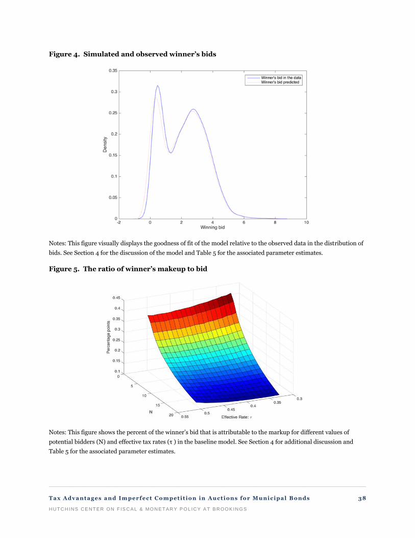
_________________________________________________________________________________________________________
Tax Adva ntages an d Im perf ect Competit ion in Auctions for Mu nicipal Bonds 38
HUT C H INS CE NT E R ON F IS C A L & MO N E T A R Y P O L IC Y A T B RO OK IN GS
Figure 4. Simulated and observed winner’s bids
Notes: This figure visually displays the goodness of fit of the model relative to the observed data in the distribution of
bids. See Section 4 for the discussion of the model and Table 5 for the associated parameter estimates.
Figure 5. The ratio of winner’s makeup to bid
Notes: This figure shows the percent of the winner’s bid that is attributable to the markup for different values of
potential bidders (N) and effective tax rates (τ ) in the baseline model. See Section 4 for additional discussion and
Table 5 for the associated parameter estimates.
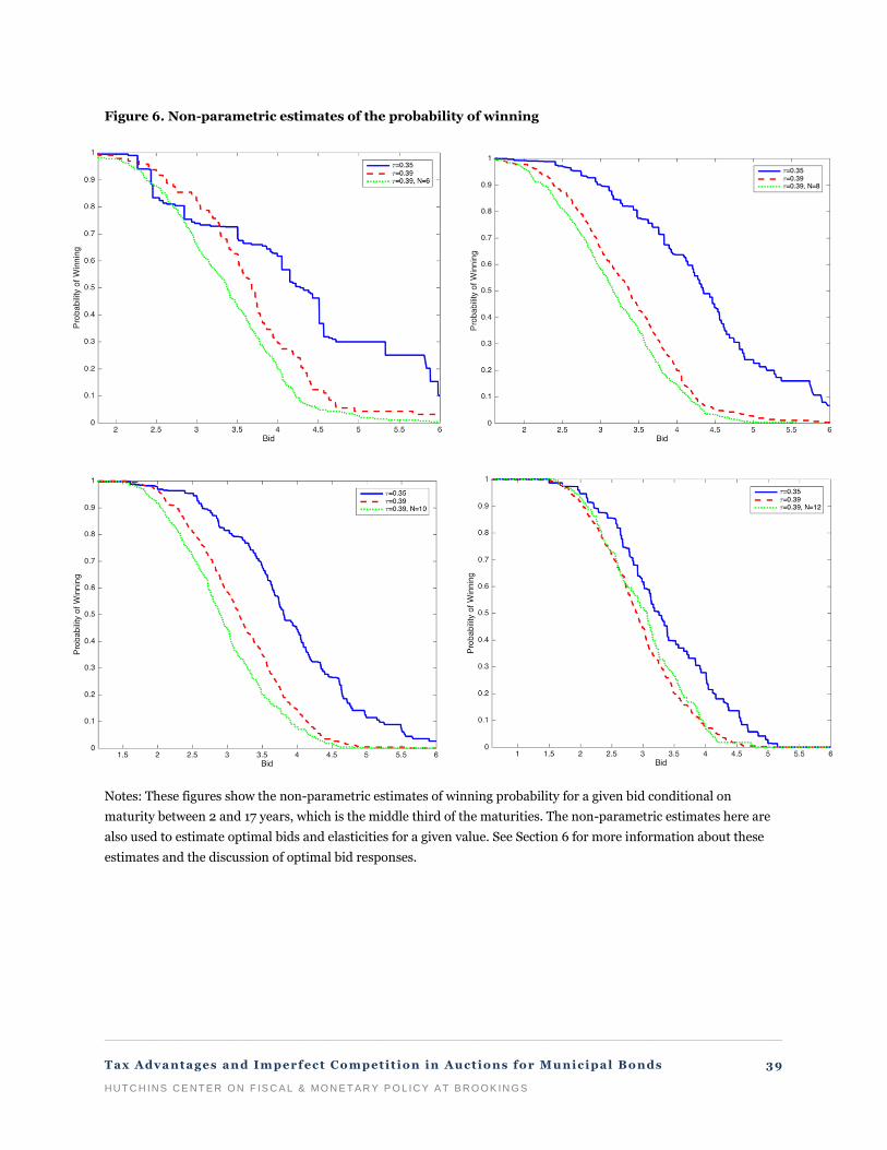
_________________________________________________________________________________________________________
Tax Adva ntages an d Im perf ect Competit ion in Auctions for Mu nicipal Bonds 39
HUT C H INS CE NT E R ON F IS C A L & MO N E T A R Y P O L IC Y A T B RO OK IN GS
Figure 6. Non-parametric estimates of the probability of winning
Notes: These figures show the non-parametric estimates of winning probability for a given bid conditional on
maturity between 2 and 17 years, which is the middle third of the maturities. The non-parametric estimates here are
also used to estimate optimal bids and elasticities for a given value. See Section 6 for more information about these
estimates and the discussion of optimal bid responses.

_________________________________________________________________________________________________________
Tax Adva ntages an d Im perf ect Competit ion in Auctions for Mu nicipal Bonds 40
HUT C H INS CE NT E R ON F IS C A L & MO N E T A R Y P O L IC Y A T B RO OK IN GS
Figure 7. 𝜶-policy outcomes for borrowing rates and markups
Notes: This figure shows counterfactual bids for different ratios of the current federal exemption. 𝛼 = 0 is equivalent
to eliminating the exemption and 𝛼 = 2 would be doubling the exemption by subsidizing municipal bond interest
income by an amount equal to the federal tax rate in addition to the exemption. See Section 7 for additional
discussion and Figures 8 and 9 for the spatial distribution of counterfactual changes associated with 𝛼 = 0.7.
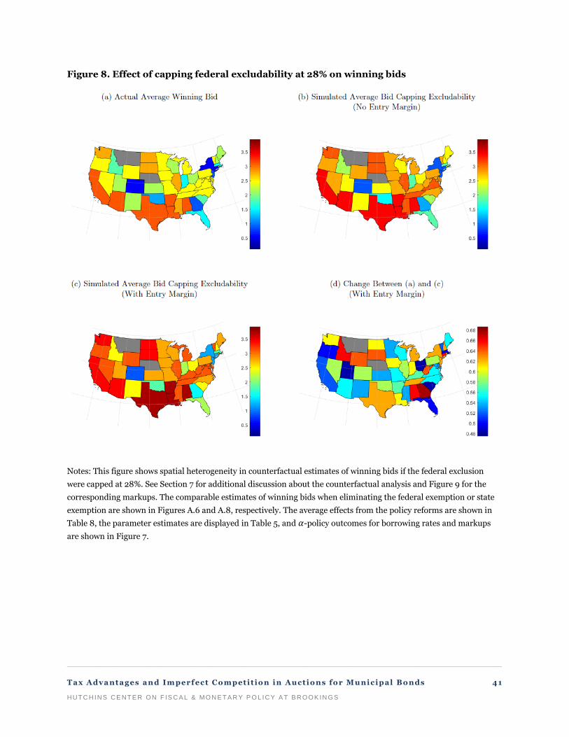
_________________________________________________________________________________________________________
Tax Adva ntages an d Im perf ect Competit ion in Auctions for Mu nicipal Bonds 41
HUT C H INS CE NT E R ON F IS C A L & MO N E T A R Y P O L IC Y A T B RO OK IN GS
Figure 8. Effect of capping federal excludability at 28% on winning bids
Notes: This figure shows spatial heterogeneity in counterfactual estimates of winning bids if the federal exclusion
were capped at 28%. See Section 7 for additional discussion about the counterfactual analysis and Figure 9 for the
corresponding markups. The comparable estimates of winning bids when eliminating the federal exemption or state
exemption are shown in Figures A.6 and A.8, respectively. The average effects from the policy reforms are shown in
Table 8, the parameter estimates are displayed in Table 5, and 𝛼-policy outcomes for borrowing rates and markups
are shown in Figure 7.

_________________________________________________________________________________________________________
Tax Adva ntages an d Im perf ect Competit ion in Auctions for Mu nicipal Bonds 42
HUT C H INS CE NT E R ON F IS C A L & MO N E T A R Y P O L IC Y A T B RO OK IN GS
Figure 9. Effect of capping federal excludability at 28% on markups
Notes: This figure shows spatial heterogeneity in counterfactual estimates of markups if the federal exclusion were
capped at 28%. See Section 7 for additional discussion about the counterfactual analysis and Figure 8 for the
corresponding bids. The comparable estimates of markups when eliminating the federal exemption or state
exemption are shown in Figures A.7 and A.9, respectively. The average effects from the policy reforms are shown in
Table 8, the parameter estimates are displayed in Table 5, and 𝛼-policy outcomes for borrowing rates and markups
are shown in Figure 7.

_________________________________________________________________________________________________________
Tax Adva ntages an d Im perf ect Competit ion in Auctions for Mu nicipal Bonds 43
HUT C H INS CE NT E R ON F IS C A L & MO N E T A R Y P O L IC Y A T B RO OK IN GS
Table 1. Descriptive statistics
Notes: More information regarding the definitions of variables included in this table is provided in Appendix A.

_________________________________________________________________________________________________________
Tax Adva ntages an d Im perf ect Competit ion in Auctions for Mu nicipal Bonds 44
HUT C H INS CE NT E R ON F IS C A L & MO N E T A R Y P O L IC Y A T B RO OK IN GS
Table 2. Reduced-form effects of the effective rate on winning bid and the number of
potential bidders
Notes: This table reports regression estimates of the effect of effective marginal tax rates on the winning bids in
municipal bond auctions between 2008 and 2015. See Section 3 for further details and Appendix A for a discussion of
the data. Additional robustness checks are discussed in Appendix C while more specifications building from this table
are presented in Table 3 with other measurement approaches shown in Table 4. The first panel showcases estimates
of effective marginal tax rates on the winning bid without controlling for the effect of competition. The second row
shows the effect that effective tax rates have on the number of potential bidders. Results with flexible controls for
competition through the number of bidders and the number of potential bidders are shown in the third panel. All
specifications include fixed effects for the state and year as well as controls for maturity, credit rating, and refund
status. Political party controls include the proportion of votes cast for the republican candidate in the most recent
senate, gubernatorial, and presidential elections in the state. Personal, Business, and Property Tax Controls include
indicators for alternative minimum taxes, exemption of instate and out-of-state federally tax-exempt debt,
deductibility of federal income taxes, corporate tax rates, property tax rates, and sales apportionment rules. Sales Tax
Controls include state sales tax rates. The natural logarithm of size of the bond package in millions of USD is included
in column (5). Standard errors clustered at the state-year level are shown in parentheses and p-values for each
estimate are displayed below standard errors.

_________________________________________________________________________________________________________
Tax Adva ntages an d Im perf ect Competit ion in Auctions for Mu nicipal Bonds 45
HUT C H INS CE NT E R ON F IS C A L & MO N E T A R Y P O L IC Y A T B RO OK IN GS
Table 3. Reduced-form effects of the effective rate on winning bid and the number of
potential bidders: Extended controls
Notes: This table presents more estimates corresponding to Table 2. The base controls include state, year,
maturity, quality, and refund status fixed effects in addition to effective rate, which is the same as column (1) in Table
2. See Appendix C for details and Appendix A for variable definitions. Standard errors clustered at the state-year level
are shown in parentheses and p-values for each estimate are displayed below standard errors.
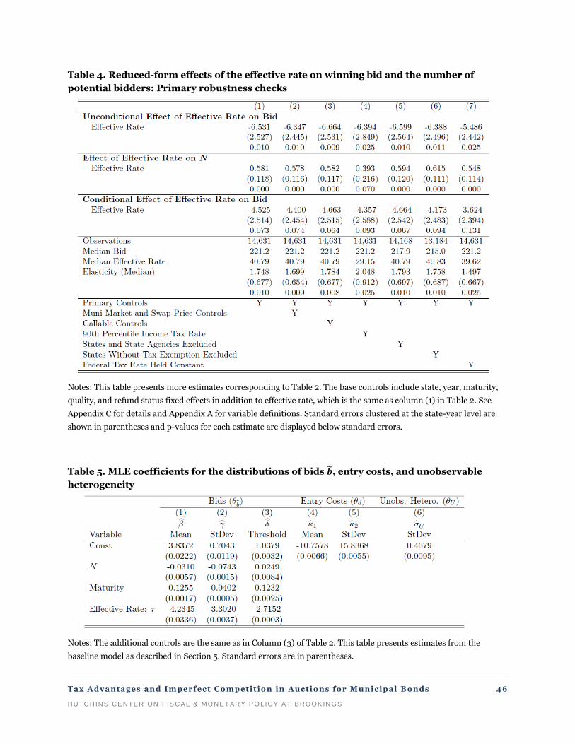
_________________________________________________________________________________________________________
Tax Adva ntages an d Im perf ect Competit ion in Auctions for Mu nicipal Bonds 46
HUT C H INS CE NT E R ON F IS C A L & MO N E T A R Y P O L IC Y A T B RO OK IN GS
Table 4. Reduced-form effects of the effective rate on winning bid and the number of
potential bidders: Primary robustness checks
Notes: This table presents more estimates corresponding to Table 2. The base controls include state, year, maturity,
quality, and refund status fixed effects in addition to effective rate, which is the same as column (1) in Table 2. See
Appendix C for details and Appendix A for variable definitions. Standard errors clustered at the state-year level are
shown in parentheses and p-values for each estimate are displayed below standard errors.
Table 5. MLE coefficients for the distributions of bids ��, entry costs, and unobservable
heterogeneity
Notes: The additional controls are the same as in Column (3) of Table 2. This table presents estimates from the
baseline model as described in Section 5. Standard errors are in parentheses.

_________________________________________________________________________________________________________
Tax Adva ntages an d Im perf ect Competit ion in Auctions for Mu nicipal Bonds 47
HUT C H INS CE NT E R ON F IS C A L & MO N E T A R Y P O L IC Y A T B RO OK IN GS
Table 6. Summary of average estimated markups by issuer type
Notes: This table showcases the average markups estimated in the structural model by issuer type. The row titled
“Total” includes all issuers including those for which an issuer type is not listed by SDC Platinum while the other rows
take the average of a subset of issuers by type. The markup is estimated directly from the model, the markup rate is
the markup divided by the winning bid, and the markup value is the markup multiplied by size and maturity. Markup
estimates are trimmed at the 2.5% level to adjust for outliers. The average bond issue has an estimated markup up of
16.8 basis points, which is 17.4% percent of their interest cost and adds up to $173,476 over the lifetime of the bond.
The issuer types are organized from higher levels of government to more local levels of government. States and state
authorities have lower markups on average that are a smaller percent of the total interest costs. The total value of the
markups for these issuers is larger because their average issue size is larger. See Section 5 for more information.
Table 7. Elasticity decomposition illustration (tax from 35% to 39%)
Notes: This table shows an example using the case of the median winning bidder in auctions with six potential
bidders. An unobservable is chosen so as to match the median bid in simulation to the median bid in the data. The
columns show the number of potential bidders, the value of the bidder, the optimal bid given the value, the
intermediate elasticity of the bid, and the intermediate elasticity of the markups. The rows of the table decompose the
change in optimal bid for the median winning bidder. The first row shows the optimal bid for a value of 1.621 and the
second row shows how the optimal bid changes if the tax rate increases by 4 percentage points but the probability of
winning is held constant. The third row allows the bidder’s own value to change as well as other bidders’ values. The
fourth row allows own and other bidder values to change as well as other bidders to enter into the auction where the
total elasticity of the bid is 1.748 and the elasticity of the markup is 6.145. For more information, see Section 6.
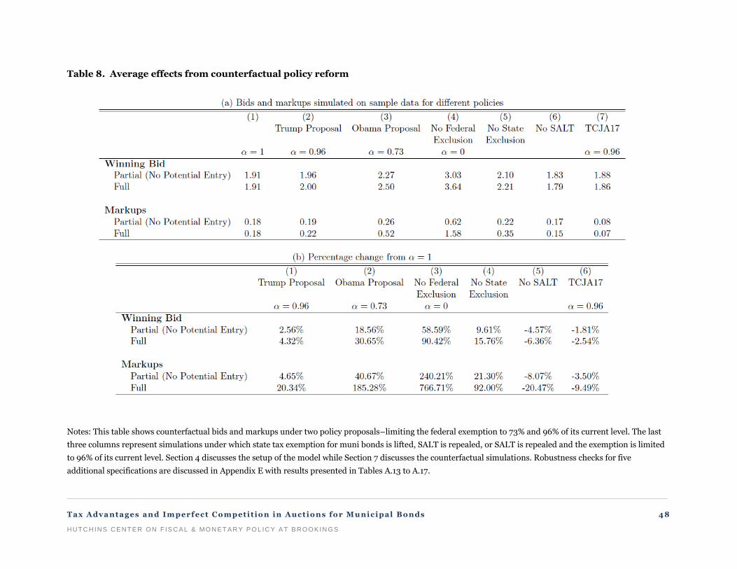
_________________________________________________________________________________________________________________________________________________
Tax Adva ntages an d Im perf ect Competit ion in Auctions for Mu nicipal Bonds 48
HUT C H INS CE NT E R ON F IS C A L & MO N E T A R Y P O L IC Y A T B RO OK IN GS
Table 8. Average effects from counterfactual policy reform
Notes: This table shows counterfactual bids and markups under two policy proposals–limiting the federal exemption to 73% and 96% of its current level. The last
three columns represent simulations under which state tax exemption for muni bonds is lifted, SALT is repealed, or SALT is repealed and the exemption is limited
to 96% of its current level. Section 4 discusses the setup of the model while Section 7 discusses the counterfactual simulations. Robustness checks for five
additional specifications are discussed in Appendix E with results presented in Tables A.13 to A.17.

_________________________________________________________________________________________________________
Tax Adva ntages an d Im perf ect Competit ion in Auctions for Mu nicipal Bonds 49
HUT C H INS CE NT E R ON F IS C A L & MO N E T A R Y P O L IC Y A T B RO OK IN GS
ONLINE APPENDIX: NOT FOR PUBLICATION
This appendix includes several sections of supplemental information. First, Appendix A contains variable
definitions for all variables used in any part of the analysis and also has a precise derivation of useful
formulas using TAXSIM variables. Appendix B describes the sample selection process. Robustness checks
to the primary reduced-form results are presented in Appendix C. The derivation of the full model is
shown in Appendix D, and robustness checks for alternative model specifications are presented in
Appendix E. Appendix F lists several potential policy reforms that motivate our counterfactual
simulations.
A. Data appendix
A.1 Variable definitions
A.1.1 Tax variables
1. State personal income tax rate. Effective top marginal personal income tax rate in each state
derived from simulated tax returns with variation across states and years. This variable is
already corrected for deductibility of federal taxes where applicable. Data from TAXSIM
(Feenberg and Coutts, 1993).
2. Federal personal income tax rate. Effective top marginal personal income tax rate at the
federal level derived from simulated tax returns. This variable is already corrected for the
deductibility of state taxes so there is variation across states and years. Data from TAXSIM
(Feenberg and Coutts, 1993).
3. Effective personal income tax rate. The sum of state and federal personal income tax rates.
Data from TAXSIM (Feenberg and Coutts, 1993).
A.1.2 Auction specific variables
1. Bid. An interest rate stated in either TIC or NIC submitted by a bidder to an auction. Data
from The Bond Buyer (2016); SDC Platinum (2016). This is scaled to be in basis points in
Tables 1 and 2.
2. Number of bidders. The number of bidders who submit bids in an auction. Data from The
Bond Buyer (2016).
3. Number of potential bidders. The number of bidders who could have submitted bids in each
auction. Data from The Bond Buyer (2016) and authors’ calculation. See Section 2.3 for the
explicit mathematical formulation.
4. Bidder and buyer. The names of banks submitting bids in each auction. The buyer is the
bidder who submits the lowest bid. Data from The Bond Buyer (2016).

_________________________________________________________________________________________________________
Tax Adva ntages an d Im perf ect Competit ion in Auctions for Mu nicipal Bonds 50
HUT C H INS CE NT E R ON F IS C A L & MO N E T A R Y P O L IC Y A T B RO OK IN GS
5. Issuer. The name and state of the municipality that is selling the bond package. Data from
The Bond Buyer (2016); SDC Platinum (2016).
6. Years (2008-2015). Indicator for the year in which the auction takes place. Data from The
Bond Buyer (2016); SDC Platinum (2016).
A.1.3 Maturity, size, quality, and refund controls
1. Maturity. The number of years between the auction and the maturity of the longest bond in
the bond package. Data from The Bond Buyer (2016).
2. Size. The size in millions of USD of the bond package. Data from The Bond Buyer (2016);
SDC Platinum (2016). In Tables 2 and A.4 the natural log of size is included instead of the
level.
3. Refund. Indicators for different refund statuses including advance refunded, current
refunded, or not refunded. Data from SDC Platinum (2016).
4. Quality. Indicators for bins of bond ratings assigned by either Moody’s or S&P. Data from
SDC Platinum (2016).
A.1.4 Political party controls
1. Governor. Percent of votes going to the Republican party in the most recent state election for
governor without counting third party votes. Data from Caesar and Saldin (2006) updated
through 2010 and imputed for future years.
2. Senate. Percent of votes going to the Republican party in the most recent senate election in
each state without counting third party votes. Data from Caesar and Saldin (2006) updated
through 2010 and imputed for future years.
3. President. Percent of votes going to the Republican party in the most recent presidential
election in each state without counting third party votes. Data from Caesar and Saldin (2006)
updated through 2010 and imputed for future years.
4. Major Party Index (MPI). The average percent of votes over 50% going to the dominant
political party across six major elections in each state calculated by Caesar and Saldin (2006).
The data are updated through 2010 and imputed for future years. MPI is not used in Table 2
but is part of the structural model controls used in Table A.4.
A.1.5 Other tax policy controls
1. Sales tax rate. Percent sales tax rate charged by the state. Data collected by Suarez Serrato
and Zidar (2016).
2. Corporate income tax rate. Percent corporate income tax rate charged by the state. Data
collected by Suarez Serrato and Zidar (2016).
_________________________________________________________________________________________________________
Tax Adva ntages an d Im perf ect Competit ion in Auctions for Mu nicipal Bonds 51
HUT C H INS CE NT E R ON F IS C A L & MO N E T A R Y P O L IC Y A T B RO OK IN GS
3. Sales Tax Apportionment Weight. Sales apportionment factor for multi-state companies,
which assigns a certain amount of a company’s income to each state for corporate income tax
purposes based on sales in that state. Data collected by Suarez Serrato and Zidar (2016).
4. Alternative minimum tax. Indicator for an alternative minimum tax in the state personal
income tax code. Data from CCH (2008-2015).
5. Federal tax deductibility. Indicator for federal taxes paid being deductible from state tax
liability.Data from CCH (2008-2015).
6. Own bond interest exempt. Indicator for personal income tax exemption of municipal bond
income from bonds that originate from within the state. Data from CCH (2008-2015).
7. Other bond interest exempt. Indicator for personal income tax exemption of municipal bond
income from bonds that originate from other states. Data from CCH (2008-2015).
A.1.6 Government spending and economic variables
1. Unemployment rate. The annual average percent of individuals currently looking for work in
each state who do not have active employment. Data from Bureau of Labor Statistics (2017).
The first difference of the unemployment rate is included in Table A.4.
2. Gross domestic product (GDP). The total economic activity in each state-year with data from
Bureau of Economic Analysis (2017). The first difference of the log of GDP is included in
Table A.4.
3. State government spending. Total annual expenditures by the state government. Data from
Census Bureau (1994-2014) with 2015 entries imputed.
4. State intergovernmental transfers. Total annual transfers from state to local governments.
Data from Census Bureau (1994-2014) with 2015 entries imputed.
5. State interest payments. Total annual interest payments for all local governments and state
agencies within a state. Data from Census Bureau (1994-2014).
6. 1-year LIBOR swap rate. The fixed rate paid on a 1-year interest rate swap. Data from Board
of Governors of the Federal Reserve System (2018).
7. 7-day municipal VRDO yield. Variable rate demand obligation yields from SIFMA is an
index of yields on a sample of large, AAA rated municipal bonds with variable rates. Data
from SIFMA (2017).
A.2 Effective rate calculations
From TAXSIM, we get variables for top marginal state and federal personal income tax rates, t s and t f
respectively. Each of these variables are already defined such that After Tax Income (ATI) can be described
as AT I = Income(1 − t f − t s). The effective tax rate is simply τ ≡ 1 − AT I/Income = t f + t s. However,

_________________________________________________________________________________________________________
Tax Adva ntages an d Im perf ect Competit ion in Auctions for Mu nicipal Bonds 52
HUT C H INS CE NT E R ON F IS C A L & MO N E T A R Y P O L IC Y A T B RO OK IN GS
the variables from TAXSIM already account for interactions of state and federal rates so they cannot be
used directly for counterfactual simulations of changes in one rate or the other.
Let Tf be the total federal tax liability and let Ts be the total state tax liability. State taxes are
always deductible from federal tax liability so Tf = tf (Income − Ts). For all but eight states, federal
taxes are not deductible from state tax liability so that Ts = tsIncome, which further implies Tf + Ts =
Income(tf (1 − ts) + ts). In this case, ATI/Income is characterized as the following:
AT I/Income = 1 − (Tf + Ts)/Income = 1 − (tf (1 − ts) + ts)
The effective rate for states that do not allow deduction of federal taxes is defined as τ = tf (1 − ts) + ts. For
states that do allow federal deduction, federal tax liability follows the same formula Tf = tf (Income−Ts) but
state taxes are now Ts = ts(Income − Tf ).
Ts = ts(Income – tf (Income − Ts))
Ts = tsIncome(1 − tf )/(1 − tstf )
This also complicates the federal tax burden.
Tf = tf (Income − T s)
Tf = tf (Income − tsIncome(1 − tf )/(1 − tstf ))
Tf = tf Income(1 − ts(1 − tf )/(1 − tstf ))
Finding 1 − AT I/Income for these states with federal deductibility yields τ = tf (1 − ts(1 − tf )/(1 − tstf
)) + ts(1 − tf )/(1 − tstf ). The remaining complication is finding ts and tf from t s and t f as presented by
TAXSIM. tf can be found by two equivalent methods. First, for states with no state-level personal
income tax, tf = t f . Secondly, for states without federal deductibility, tf = t f /(1 − t s). For states without
federal deductibility, the actual tax rate is trivially equivalent to the TAXSIM reported rate. For states
with federal deductibility:
t s = ts(1 − tf )/(1 − tstf )
t s = ts − tstf + tststf
⇒ ts = t s/(1 − tf + t stf )
The underlying tax rates and the counterfactual effective rate can be calculated directly from ts and tf .
If a state does not exempt interest on their own bonds, then state taxes are still paid on interest and the
effective rate of the exemption is equal to the federal rate corrected for the state tax deduction.

_________________________________________________________________________________________________________
Tax Adva ntages an d Im perf ect Competit ion in Auctions for Mu nicipal Bonds 53
HUT C H INS CE NT E R ON F IS C A L & MO N E T A R Y P O L IC Y A T B RO OK IN GS
B. Sample construction
The combined Bond Buyer and SDC data represent 41,918 competitive auctions issued between February
2008 and December 2015 worth a total $589.9 billion. There is significant variation in the structure of the
bond packages on several different dimensions. Most notably, the size of the bonds varies from $10
thousand to $950 million with a median value of $4.05 million. 91.8% of the market value comes from
issuances of more than $5 million. The interest rates paid by municipalities range from 0.005% to 8.5%
with a median rate of 2.16%. Maturities range from less than one year to 40 years with a median maturity
of 10 years.
Bonds can be funded by either “General Obligation” (GO) or “Revenue” (RV). GO bonds are paid back
using any financing capacity of the municipality. GO bonds are more commonly used to finance roads,
public schools, and low-income housing units that beneficiaries do not pay fees to utilize. Among the
bonds in the combined data 4,220 (10.07%) are RV bonds, and the remaining 37,698 (89.93%) are GO
bonds.
From the total set of municipal bond auctions in our data, we create the sample we analyze by
dropping: RV bonds, bonds for which we lack important information (like maturity or size), bonds with
total size less than $5 million, taxable municipal bonds, and Build America Bonds (BABs).48
The step-by-
step outcomes of our sample construction are shown in Tables A.1 and A.2.
After merging the SDC Platinum and Bond Buyer data, we are left with 15,354 auctions. Of those, 433
are dropped for being issued in 2016 for which we don’t have corresponding TAXSIM data and 290 are
dropped for missing the winning bid. The final analysis sample is made up of 14,631 auctions from 2008
to 2015.
C. Robustness of reduced-form results
C.1 Additional specifications detailing effect of taxes on winning bid
Table A.4 builds on the main specifications presented in Table 2 with additional controls. Column (1) is
the same across tables for comparison where base controls include state and year fixed effects, maturity
fixed effects, size controls, quality fixed effects, and refund status fixed effects. Column (2) presents a new
specification that uses controls for state and year fixed effects, maturity fixed effects, corporate tax rates,
property tax rates, sales tax rates, presidential, gubernatorial, and senate voting records, and major party
index. Nebraska is missing MPI data so its 18 auctions are dropped from specifications with structural
model controls. These are the same controls as those used in Section 5.2. Column (3) uses every control in
the robustness table plus every control in Table 3. The estimated coefficients are very stable between 6.5
and 6.7 basis points across all specifications without controls for number of actual or potential bidders.
With controls for actual and potential bidders shown in the third panel, estimates still only vary from 4.5
to 5.4 basis points.
. . .
48. The American Recovery and Reinvestment Act of 2009 created an additional class of taxable municipal debt: BABs. The return
to the investor in BABs is taxable but the federal government partially reimburses municipalities for the interest cost incurred.
These bonds show up in the data from 2009-2011, but we exclude them from our analysis as demand for these bonds will not
be directly influenced by tax policy.

_________________________________________________________________________________________________________
Tax Adva ntages an d Im perf ect Competit ion in Auctions for Mu nicipal Bonds 54
HUT C H INS CE NT E R ON F IS C A L & MO N E T A R Y P O L IC Y A T B RO OK IN GS
Table A.5 shows additional specifications of the regression equation estimated in Table 2. Columns (1)
to (4) show different versions of the choice of standard errors. We use standard errors clustered at the
state-year level in the main specifications, which are more conservative than standard errors clustered at
the state-month level and robust standard errors. Columns (5) and (6) show the robustness of the results
to monthly and daily fixed effects, respectively. The specification in Column (7) expands the sample
universe to include all bonds sold at auction including those for less than $5 million. The specification
including small bonds is weighted by size bins.
C.2 Effect of taxes on potential and actual bidders
Panel B in Table 2 shows that our preferred definition of potential bidders is responsive to changes in the
tax advantage. We explore whether this result also holds for the number of actual bidders as well as for
alternative definition of the number of potential bidders. Table A.6 shows similar results for the actual
number of bidders, as well as our alternative definition of potential bidders. The effects on these panels
are stable across specifications and are statistically significant in most cases. As expected, the values of the
coefficient vary across definitions of potential bidders, as some definitions are broader and include
bidders that may have very little chance of responding to the change in taxes.
C.3 Effect of taxes on supply of municipal debt
We explore whether changes in the effective rate affect the supply for municipal bonds. Adelino et al.
(2017) find that supply of municipal debt increases at the local level when the cost of debt decreases on
the intensive margin but not the extensive margin. Since we control for the size of the bond, we are
primarily concerned with any supply response on the extensive margin. Table A.7 shows that the supply of
municipal debt is not responsive to changes in effective tax rates.
C.4 Heterogeneous effects by bond length
The main reduced-form results in Table 2 assume the coefficient of the effective rate on the borrowing
cost is homogeneous across characteristics of the bonds. We explore whether this is a good assumption by
allowing for the effect to vary by bond length. Figure A.4 shows the empirical distribution of bond length.
If the effect of the tax advantage varies by bond length, the estimates in Table 2 may be biased. Figure A.5
shows estimated coefficients of the effective rate on winning bid by length of bond. This specification
controls for all our main controls including bidder fixed effects and corresponds to Column (4) of Table 2.
This figure shows there is some variance on effects with larger effects in the first two years and more
variable effects in later years. Table A.8 estimates the Average Partial Effect and the effect from the Fixed
Effect model using a weighting estimator in Gibbons et al. (2014). While the effects in Figure A.5 vary a lot,
the interactions between the length indicators and the effective rate are not statistically significant,
according to the score test p-value. The APE and FE estimates are also not statistically different, according
to the Hausman test p-value. The fraction due to competition is slightly smaller in the APE, 23%, versus
28% in the FE. These results suggest that the assumption of homogeneous coefficients is not biasing our
main results.

_________________________________________________________________________________________________________
Tax Adva ntages an d Im perf ect Competit ion in Auctions for Mu nicipal Bonds 55
HUT C H INS CE NT E R ON F IS C A L & MO N E T A R Y P O L IC Y A T B RO OK IN GS
C5. Coefficient stability robustness tests
In Tables 2 and A.4 we provide evidence of coefficient stability across several specifications with different,
sequentially-added controls. However, Altonji et al. (2005) and Oster (2017) have pointed out that
coefficient stability is not sufficient to show that omitted variable bias, or selection on unobservables, has
been negated. These papers introduce a new way to think about coefficient stability and several ways to
test for the robustness of results.
The intuition is that the relative changes in estimated coefficients when more regressors are added
can be used to correct for omitted variable bias. Changes in R2 should be used to scale changes in
estimates of β when additional regressors are being added sequentially. In order to test the validity of our
coefficient stability as a signal of mitigated omitted variable bias, we implement one of the estimators
from Oster (2017). The following is helpful notation used to define the estimator:
�� and ��. The estimates of β and R2
from a regression with base controls.
𝛽 and ��. The estimates of β and R2 from a regression with additional controls.
β∗. The bias-adjusted estimate of β.
δ. “Coefficient of Proportionality” or proportion of variation in the main control of interest
explainable by unobservables.
Rmax. The maximum R2 attainable with perfect controls.
Parameters δ and Rmax are not observable, so we assume that both are equal to one following the
guidance of Oster (2017). There are two primary ways to implement the estimator: 1) estimate β∗ for a
given δ and Rmax, or 2) estimate the δ that sets β∗ = 0 given Rmax. The former gives an unbiased estimate of
the causal effect of the variable of interest on the dependent variable. The latter is interpreted as the
importance of unobservables that would be needed to negate the observed effect entirely. The following is
the estimator from which corrected estimates can be calculated given δ, or δ can be calculated for a given
β∗:
𝛽∗ ≈ 𝛽 − 𝛿[�� − 𝛽]𝑅𝑚𝑎𝑥 − ��
�� − ��
We include calculations of both the δ that would be needed to set β∗ = 0, and the β
∗ implied by the
assumption that δ = 1 in Table A.9. We set Rmax = 1 for all specifications.
For columns (1) and (2), the estimates of δ are negative and the corrected estimates for δ = 1 are
greater than the original estimates. These results arise from the increase in the magnitude of the estimate
when more controls are added. In column (3), the estimate attenuates toward zero slightly while R2
increases with additional controls. The estimate of δ is 113.9, which is much larger than the cutoff
threshold of 1 suggested in Oster (2017). The interpretation of this estimate is that selection on
unobservables would need to be 113.9 times more important than selection on observables for our results
to be negated. The results of this test highlight that selection on unobservables would need to be very large
to negate the results presented in Tables 2 and A.4.
C.6 Effect of interest costs on tax rates (reverse causality)
As discussed in Section 3, there is a potential that states could adjust tax rates to deal with changes in
local borrowing cost such as raising revenue to cover past or future increases in interest rates. To
investigate this possibility we gather data from Census Bureau (1994-2014) on total interest payments

_________________________________________________________________________________________________________
Tax Adva ntages an d Im perf ect Competit ion in Auctions for Mu nicipal Bonds 56
HUT C H INS CE NT E R ON F IS C A L & MO N E T A R Y P O L IC Y A T B RO OK IN GS
made by governments in each state from 1994 to 2004 and regress tax rates on these interest payments as
well as leads and lags of interest payments. Tables A.10 and A.11 show that interest payments are not
associated with a change in tax rates.
D. Detailed model derivation
In this section we consider an auction with N potential bidders. As with most standard results in the
auctions literature, we assume here that valuations of bidders are distributed over some compact support
[v, ��], that they are jointly affiliated, and that their density f (v) is continuously differentiable.
First, we assume existence of a differentiable monotone equilibrium bidding strategy β(v). Suppose
some agent i decides to enter the auction. At the bidding stage, i solves maximization problem
max𝑣′(𝛽(𝑣′) − 𝑣𝑖)𝑷𝑟[𝑣−𝑖 > 𝑣′]
where 𝒗−𝒊 denotes all values among the potential competitors. This problem essentially suggests that i
optimally chooses to bid as if she had value 𝑣′, while all other agents bid according to the strategy β(·). In
Nash Equilibrium, it must be that v’ = 𝑣𝑖 .
This maximization problem generates the first order condition
𝛽′(𝑣)𝑷𝑟[𝑣−𝑖 > 𝑣] + (𝛽(𝑣) − 𝑣)𝜕𝑷𝑟[𝑣−𝑖 > 𝑣]
𝜕𝑣= 0
where 𝑣′ = v = 𝑣𝑖 when β(·) solves for equilibrium. This is a first order differential equation for β(·). A
slight complication arises due to lack of a border condition which would allow us to solve the equation.
We pick a specific equilibrium in which the participant with the highest valuation bids precisely her own
valuation. In this case, the unique solution to the maximization problem can be represented as
𝛽(𝑣) = 𝑣 +∫ 𝑷𝑟[𝑣−𝑖 > 𝑠]𝑑𝑠𝑣
𝑣
𝑷𝑟[𝑣−𝑖 > 𝑣].
This equation represent the unique monotone smooth equilibrium bidding strategy under our assumption
β(��) = ��.49
We denote the corresponding profits as
𝜋(𝑣) = (𝛽(𝑣) − 𝑣)𝑷𝑟[𝑣−𝑖 > 𝑣].
Note that these profits implicitly depend on the probability with which agents enter the auction through
the right-hand side expression P𝑟[𝑣−𝑖> v].
At the participation stage of the game, agent i facing costs di enters iff
∫𝜋(𝑣)𝑓(𝑣)𝑑𝑣 ≥ 𝑑𝑖.
��
𝑣
We assume that di are i.i.d., which allows us to define
. . .
49. In fact, other equilibria with smooth bidding strategies are not as natural because they feature β(𝑣) = +∞

_________________________________________________________________________________________________________
Tax Adva ntages an d Im perf ect Competit ion in Auctions for Mu nicipal Bonds 57
HUT C H INS CE NT E R ON F IS C A L & MO N E T A R Y P O L IC Y A T B RO OK IN GS
𝑝∗ = 𝑷𝑟(𝑖 𝑒𝑛𝑡𝑒𝑟𝑠 𝑡ℎ𝑒 𝑎𝑢𝑐𝑡𝑖𝑜𝑛) = 𝑷𝑟 (𝑑𝑖 ≤ ∫𝜋(𝑣)𝑓(𝑣)𝑑𝑣
��
𝑣
) = 𝐻(∫𝜋(𝑣)𝑓(𝑣)𝑑𝑣
��
𝑣
),
where H(·) is the CDF of entry costs. With p∗ defined, we impose the equilibrium restriction on the whole
entry-bidding game in the form of
𝑷𝑟[𝑣−𝑖 > 𝑣] = 𝐶𝑁−10 (1 − 𝑝∗)𝑁−1(1 − 𝐹(𝑣)) + ∑𝐶𝑁−1
𝑗
𝑁−1
𝑗=1
(1 − 𝑝∗)𝑁−1−𝑗(𝑝∗)𝑗(1 − 𝐹(𝑣))𝑗,
which is a result of the assumption that in absence of other entrants the sole auction participant competes
with the seller.
E. Robustness of structural estimates
We now show that our implications for passthrough elasticities, markups, and counterfactual policies are
robust to different model specifications. The model fit and markups are presented in Table A.12 for all
robustness checks to the structural model. We estimate the following models:
S1 This is our baseline model, but where the mean is a flexible piecewise-linear function of
N and maturities, as opposed to the linear case in the baseline model.
In particular, if µb = Xβ is the representation of the mean parameter for bids in the baseline
model, in the piecewise-linear mean model we have
𝜇𝑏 = 𝑋�� +∑(𝟏(𝑁𝑖−1 ≤ 𝑁 < 𝑁𝑖) [𝛽𝑁,𝑖(𝑁 − 𝑁𝑖−1) +∑𝛽𝑁,𝑗(𝑁𝑗 −𝑁𝑗−1)
𝑖−1
𝑗=1
])
𝑘
𝑖=1
where 𝑋�� represents the portion of the mean which does not include N as a dependent
variable, and points Ni partition the support of N in the sample so that 0 = N0 < N1 < . . . < Nk .
Coefficients 𝛽𝑁,𝑖 are simply slopes of µb in N when N lies in [Ni−1, Ni). In practice, we have k =
4, and the intermediary Ni are chosen as quartiles of the distribution of N in our data sample.
An equivalent construction is used for maturities.
The policy simulations are presented in Table A.13. This approach allows us to see if the best
fit is non-linear in N and maturities. The estimated passthrough elasticities, markups, and
policy implications are very similar to our baseline model.
S2 Baseline model, but where N is defined as the number of unique bidders across all
auctions within a given state in a given month. The policy simulations are presented in Table
A.14. These tables present similar results to our baseline model. This definition of potential
bidders mechanically implies lower entry on average, and our model matches this pattern
quite closely.
S3 Baseline model, but we restrict the threshold parameter to 0 for all auctions. The policy
simulations are presented in Table A.15. These tables present evidence that our results are not
sensitive to issues that may arise when the support of the variables depends on the estimated
parameters.

_________________________________________________________________________________________________________
Tax Adva ntages an d Im perf ect Competit ion in Auctions for Mu nicipal Bonds 58
HUT C H INS CE NT E R ON F IS C A L & MO N E T A R Y P O L IC Y A T B RO OK IN GS
S4 Baseline model, but where the effect of Effective Rate τ on standard deviation of bids set
to 0. The policy simulations are presented in Table A.16. These tables show that our results
are not solely dependent on the effect of the tax advantage on the dispersion of bids. As
discussed in the paper, the effect of the tax advantage on the dispersion of bids may have
countervailing implications for the markup and selection effects which, in this case, result in
similar effects for our counterfactual policies.
S5 Baseline model, but where we truncate the distribution of bids at the entry stage. One
potential concern is that the inclusion of the full support of distribution of bids in the
calculations for expected profits at the entry stage may artificially generate high entry costs,
which may bias our results. As a robustness check, we re-estimate the baseline mode by
excluding 0.1% of bid support from its left tail. Precisely, we assume that
𝐸𝜋(𝑝) = ∫ 𝑔(𝑏)𝜋(𝑏|𝑝)𝑑𝑏
∞
𝑞𝑏(0.001)
(10)
where p denote the probability of entry and qb(0.001) is the 0.001-quantile for the
distribution of b. We obtain similar policy implications, which are presented in Table A.17,
and model fit and markups, which are presented in Table A.12. The estimated average entry
margin threshold is slightly lower in this specification.
F. Proposed reforms
There are several recent and current tax reform proposals at the federal level that would change the
borrowing cost of municipalities and demand for municipal debt. Broadly speaking, proposed reforms fit
into 3 categories: changing the federal tax rate of the exemption, permanently introducing other types of
subsidized municipal debt like Build America Bonds, and changing the scope of projects that are allowed
to be tax exempt. The first of these categories is the primary focus of this paper and captures most reforms
that have been proposed.
Both Democrats and Republicans have proposed plans in recent years that will decrease the size of the
tax exemption received by municipal bonds. In the Tax Cut and Jobs Act of 2017, the top marginal rate
was cut from 39.6% down to 37%. Former President Obama proposed a larger cut to the municipal bond
interest exemption in particular without necessarily adjusting the top statutory federal income tax rate.
The Obama White House first proposed a cap in the municipal bond exemption at 28% in the American
Jobs Act of 2011 and then in budget proposals in the subsequent years (National Governors Association,
2012). These specific policy proposals provide the motivation for the choices of federal income tax ratesin
the counterfactual simulations at 𝛼 = 0.28
0.386 ≈ 0.73 and 𝛼 =
0.37
0.386≈ 0.96 where 0.386 is marginal rate in the
subsample for years 2011-2015.
Other reforms to the supply of municipal bonds to extend the availability of Build America Bond
subsidies or to tighten tax-exempt eligibility are discussed among scholars and think-tanks but have not
been formally proposed to our knowledge. Puentes et al. (2013) suggests that BABs are superior to
traditional municipal bonds on several margins, which is echoed in some of the academic literature
including Liu and Denison (2014). Government Finance Officers Association (2000) discusses the

_________________________________________________________________________________________________________
Tax Adva ntages an d Im perf ect Competit ion in Auctions for Mu nicipal Bonds 59
HUT C H INS CE NT E R ON F IS C A L & MO N E T A R Y P O L IC Y A T B RO OK IN GS
potential effects of legislation in the spirit of the Tax Reform Act of 1986 that kept many bond issues from
qualifying for tax exemption.

____________________________________________________________________________________________________________________
Tax Adva ntages an d Im perf ect Competit ion in Auctions for Mu nicipal Bonds 60
HUT C H INS CE NT E R ON F IS C A L & MO N E T A R Y P O L IC Y A T B RO OK IN GS
APPENDIX GRAPHS
Figure A.1. Frequency of auctions by (N, τ ) pairs
Notes: This figure shows the frequency of observations by number of potential bidders (N) and bins of effective tax rate. See
Section 2 for more information about the data and variables.

____________________________________________________________________________________________________________________
Tax Adva ntages an d Im perf ect Competit ion in Auctions for Mu nicipal Bonds 61
HUT C H INS CE NT E R ON F IS C A L & MO N E T A R Y P O L IC Y A T B RO OK IN GS
Figure A.2. Number of bidder fixed effects and distribution of number of bidders
Notes: This figure shows the number of bidder fixed effect estimates from specification (4) of Table 2 normalized to the median
bid in addition to the empirical distribution of the number of bidders in our sample. The reduced-form analysis is discussed in
Section 3 and robustness checks are presented in Appendix C.

____________________________________________________________________________________________________________________
Tax Adva ntages an d Im perf ect Competit ion in Auctions for Mu nicipal Bonds 62
HUT C H INS CE NT E R ON F IS C A L & MO N E T A R Y P O L IC Y A T B RO OK IN GS
Figure A.3. Number of potential bidder fixed effects and distribution of number of potential bidders
Notes: This figure shows the frequency of observations by number of potential bidders (N) and the associated fixed effect
estimates from Table 2, column (4). See Section 3 for discussion of the reduced-form model.

____________________________________________________________________________________________________________________
Tax Adva ntages an d Im perf ect Competit ion in Auctions for Mu nicipal Bonds 63
HUT C H INS CE NT E R ON F IS C A L & MO N E T A R Y P O L IC Y A T B RO OK IN GS
Figure A.4. Empirical distribution of bond lengths
Notes: This figure shows the frequency of observations by length of bond. We test for heterogeneity of effect by length of bond in
the reduced-form model in Appendix C.
Figure A.5. Effect of effective rate on winning bid by length of bond
Notes: This figure shows the estimated coefficients of effect of effective rate on winning bid. See Appendix C form more
information and Table A.8 for the associated statistical tests.

_________________________________________________________________________________________________________________________________________________________________
Tax Adva ntages an d Im perf ect Competit ion in Auctions for Mu nicip al Bonds 64
HUT C H INS CE NT E R ON F IS C A L & MO N E T A R Y P O L IC Y A T B RO OK IN GS
Figure A.6. Effect of removing federal excludability on winning bids
Notes: This figure shows spatial heterogeneity in counterfactual estimates of markups if the federal exclusion was removed. See Section 7 for additional discussion and Figure A.7 for
the corresponding markups. The comparable estimates of winning bids when capping the federal exemption at 28% is shown in Figure 8. The average effects from the policy reforms
are shown in Table 8, the parameter estimates are displayed in Table 5, and federal 𝛼-policy outcomes for borrowing rates and markups are shown in Figure 7.

_________________________________________________________________________________________________________________________________________________________________
Tax Adva ntages an d Im perf ect Competit ion in Auctions for Mu nicip al Bonds 65
HUT C H INS CE NT E R ON F IS C A L & MO N E T A R Y P O L IC Y A T B RO OK IN GS
Figure A.7. Effect of removing federal excludability on markups
Notes: This figure shows spatial heterogeneity in counterfactual estimates of markups if the federal exclusion was removed. See Section 7 for additional discussion and Figure A.6 for
the corresponding bids. The comparable estimates of markups when capping the federal exemption at 28% is shown in Figure 9. The average effects from the policy reforms are
shown in Table 8, the parameter estimates are displayed in Table 5, and federal 𝛼-policy outcomes for borrowing rates and markups are shown in Figure 7.
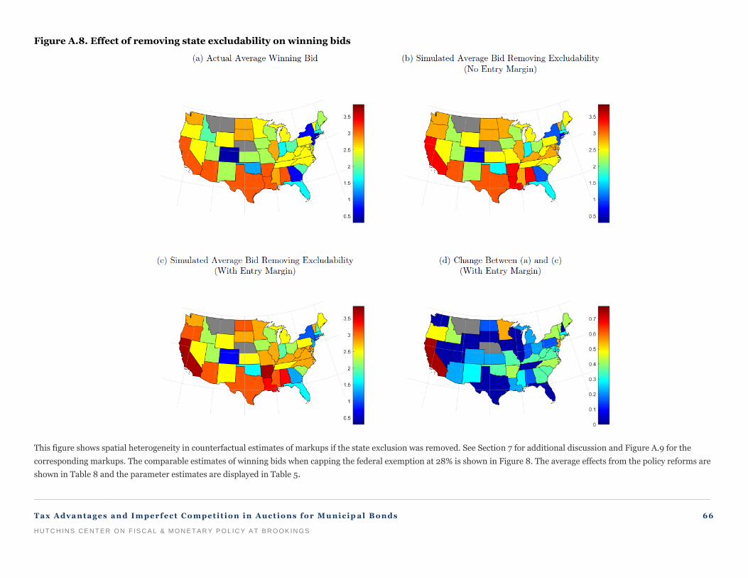
_________________________________________________________________________________________________________________________________________________________________
Tax Adva ntages an d Im perf ect Competit ion in Auctions for Mu nicip al Bonds 66
HUT C H INS CE NT E R ON F IS C A L & MO N E T A R Y P O L IC Y A T B RO OK IN GS
Figure A.8. Effect of removing state excludability on winning bids
This figure shows spatial heterogeneity in counterfactual estimates of markups if the state exclusion was removed. See Section 7 for additional discussion and Figure A.9 for the
corresponding markups. The comparable estimates of winning bids when capping the federal exemption at 28% is shown in Figure 8. The average effects from the policy reforms are
shown in Table 8 and the parameter estimates are displayed in Table 5.

_________________________________________________________________________________________________________________________________________________________________
Tax Adva ntages an d Im perf ect Competit ion in Auctions for Mu nicip al Bonds 67
HUT C H INS CE NT E R ON F IS C A L & MO N E T A R Y P O L IC Y A T B RO OK IN GS
Figure A.9. Effect of removing state excludability on markups
Notes: This figure shows spatial heterogeneity in counterfactual estimates of markups if the state exclusion was removed. See Section 7 for additional discussion and Figure A.8 for
the corresponding bids. The comparable estimates of markups when capping the federal exemption at 28% is shown in Figure 9. The average effects from the policy reforms are
shown in Table 8 and the parameter estimates are displayed in Table 5.

_________________________________________________________________________________________________________________________________________________________________
Tax Adva ntages an d Im perf ect Competit ion in Auctions for Mu nicip al Bonds 68
HUT C H INS CE NT E R ON F IS C A L & MO N E T A R Y P O L IC Y A T B RO OK IN GS
Figure A.10. Effect of repealing SALT on winning bids
Notes: This figure shows spatial heterogeneity in counterfactual estimates of markups if the SALT deduction was removed. See Section 7 for additional discussion and Figure A.11 for
the corresponding markups. The comparable estimates of winning bids when capping the federal exemption at 28% is shown in Figure 8. The average effects from the policy reforms
are shown in Table 8 and the parameter estimates are displayed in Table 5.
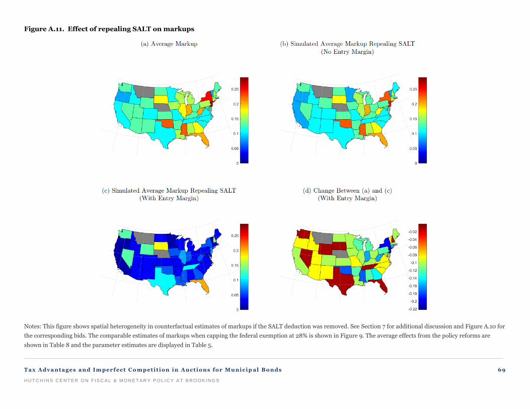
_________________________________________________________________________________________________________________________________________________________________
Tax Adva ntages an d Im perf ect Competit ion in Auctions for Mu nicip al Bonds 69
HUT C H INS CE NT E R ON F IS C A L & MO N E T A R Y P O L IC Y A T B RO OK IN GS
Figure A.11. Effect of repealing SALT on markups
Notes: This figure shows spatial heterogeneity in counterfactual estimates of markups if the SALT deduction was removed. See Section 7 for additional discussion and Figure A.10 for
the corresponding bids. The comparable estimates of markups when capping the federal exemption at 28% is shown in Figure 9. The average effects from the policy reforms are
shown in Table 8 and the parameter estimates are displayed in Table 5.

_________________________________________________________________________________________________________________________________________________________________
Tax Adva ntages an d Im perf ect Competit ion in Auctions for Mu nicip al Bonds 70
HUT C H INS CE NT E R ON F IS C A L & MO N E T A R Y P O L IC Y A T B RO OK IN GS
Figure A.12. Effect of repealing SALT and capping federal excludability at 37% on winning bids
Notes: This figure shows spatial heterogeneity in counterfactual estimates of markups if the SALT deduction was removed and federal excludability capped at 37%. See Section 7 for
additional discussion and Figure A.13 for the corresponding markups. The comparable estimates of winning bids when only SALT is repealed are shown in Figure A.10. The average
effects from the policy reforms are shown in Table 8 and the parameter estimates are displayed in Table 5.

_________________________________________________________________________________________________________________________________________________________________
Tax Adva ntages an d Im perf ect Competit ion in Auctions for Mu nicip al Bonds 71
HUT C H INS CE NT E R ON F IS C A L & MO N E T A R Y P O L IC Y A T B RO OK IN GS
Figure A.13. Effect of repealing SALT and capping federal excludability at 37% on markups
Notes: This figure shows spatial heterogeneity in counterfactual estimates of markups if the SALT deduction was removed. See Section 7 for additional discussion and Figure A.12 for
the corresponding bids. The comparable estimates of markups when only SALT is repealed are shown in Figure A.11. The average effects from the policy reforms are shown in Table 8
and the parameter estimates are displayed in Table 5.

_________________________________________________________________________________________________________
Tax Adva ntages an d Im perf ect Competit ion in Auctions for Mu nicipal Bonds 72
HUT C H INS CE NT E R ON F IS C A L & MO N E T A R Y P O L IC Y A T B RO OK IN GS
APPENDIX TABLES
Table A.1. Waterfall table for SDC data
Notes: This table shows observations that were dropped in each step of the data cleaning procedure for the SDC
Platinum data. See Appendix B for details.
Table A.2. Waterfall table for Bond Buyer data
Notes: This table shows observations that were dropped in each step of the data cleaning procedure for the Bond
Buyer data. See Appendix B for details.
Table A.3. Waterfall for data merge
Notes: This table shows the merge between SDC Platinum and Bond Buyer data. See Appendix B for details.

_________________________________________________________________________________________________________
Tax Adva ntages an d Im perf ect Competit ion in Auctions for Mu nicipal Bonds 73
HUT C H INS CE NT E R ON F IS C A L & MO N E T A R Y P O L IC Y A T B RO OK IN GS
Table A.4. Reduced-form effects of the effective rate on winning bid and the number of
potential bidders: Robustness checks part 1
Notes: This table presents more estimates corresponding to Table 2. The base controls include state, year, maturity,
quality, and refund status fixed effects in addition to effective rate, which is the same as column (1) in Table 2. See
Appendix C for details and Appendix A for variable definitions. Standard errors clustered at the state-year level are
shown in parentheses and p-values for each estimate are displayed below standard errors.
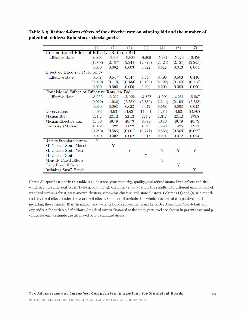
_________________________________________________________________________________________________________
Tax Adva ntages an d Im perf ect Competit ion in Auctions for Mu nicipal Bonds 74
HUT C H INS CE NT E R ON F IS C A L & MO N E T A R Y P O L IC Y A T B RO OK IN GS
Table A.5. Reduced-form effects of the effective rate on winning bid and the number of
potential bidders: Robustness checks part 2
Notes: All specifications in this table include state, year, maturity, quality, and refund status fixed effects and size,
which are the same controls in Table 2, column (5). Columns (1) to (4) show the results with different calculations of
standard errors–robust, state-month clusters, state-year clusters, and state clusters. Columns (5) and (6) use month
and day fixed effects instead of year fixed effects. Column (7) includes the whole universe of competitive bonds
including those smaller than $5 million and weights bonds according to size bins. See Appendix C for details and
Appendix A for variable definitions. Standard errors clustered at the state-year level are shown in parentheses and p-
values for each estimate are displayed below standard errors.
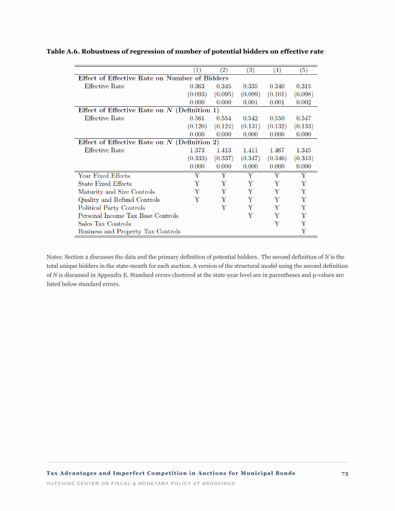
_________________________________________________________________________________________________________
Tax Adva ntages an d Im perf ect Competit ion in Auctions for Mu nicipal Bonds 75
HUT C H INS CE NT E R ON F IS C A L & MO N E T A R Y P O L IC Y A T B RO OK IN GS
Table A.6. Robustness of regression of number of potential bidders on effective rate
Notes: Section 2 discusses the data and the primary definition of potential bidders. The second definition of N is the
total unique bidders in the state-month for each auction. A version of the structural model using the second definition
of N is discussed in Appendix E. Standard errors clustered at the state-year level are in parentheses and p-values are
listed below standard errors.

_________________________________________________________________________________________________________
Tax Adva ntages an d Im perf ect Competit ion in Auctions for Mu nicipal Bonds 76
HUT C H INS CE NT E R ON F IS C A L & MO N E T A R Y P O L IC Y A T B RO OK IN GS
Table A.7. Effect of effective rate on supply of bond auctions
Notes: This table shows regressions of the supply of municipal debt as measured by the natural log of the number of
bond offerings on effective tax rates. The specifications mirror the specifications used in Table 2 except only state-
level variables are used. The dependent variable is the natural log of the number of bond issues in a given state-month
so zeros are not included. However, the failure to reject the zero effect is robust to OLS in levels, Poisson, and defining
the dependent variable to be the natural log of the count plus one. Column (1) controls for state and month fixed
effects. Column (2) adds controls for political parties while column (3) additionally adds personal income tax bases,
corporate tax rate and base controls, and average property tax rates. All of the controls mentioned above and sales tax
rates are included in column (4). See Section 3 and Appendix C for more information. Standard errors clustered at the
state-year level are shown in parentheses with p-values listed below standard errors.

_________________________________________________________________________________________________________
Tax Adva ntages an d Im perf ect Competit ion in Auctions for Mu nicipal Bonds 77
HUT C H INS CE NT E R ON F IS C A L & MO N E T A R Y P O L IC Y A T B RO OK IN GS
Table A.8. Effect of effective rate on winning bid: APE and FE
Notes: Standard errors are shown in parentheses with p-values below standard errors. See Appendix C for
information about testing for heterogeneous effects in length. This table presents the estimates that correspond to
Figure A.5 and shows the Hausman test p-value for the difference between the average partial effect and fixed effect
estimates, which is insignificant at conventional levels.

_________________________________________________________________________________________________________
Tax Adva ntages an d Im perf ect Competit ion in Auctions for Mu nicipal Bonds 78
HUT C H INS CE NT E R ON F IS C A L & MO N E T A R Y P O L IC Y A T B RO OK IN GS
Table A.9. Oster coefficient stability tests
Notes: Standard errors clustered at the state level are shown in parentheses and p-values are below standard errors.
This table uses an estimator from Oster (2017) to test how much selection on unobservables is needed to negate the
results in Tables 2 and A.4. Each cell represents the results of a previously estimated model. Under some assumptions
on the nature of selection discussed in Oster (2017), columns (1) and (2) show that no amount of unobserved
heterogeneity will negate the observe coefficients. The δ shown in column (3) implies that selection on unobservables
would need to be 113.4 times more important than selection on observables for our results to be negated. For more
information see Appendix C.5.

_________________________________________________________________________________________________________
Tax Adva ntages an d Im perf ect Competit ion in Auctions for Mu nicipal Bonds 79
HUT C H INS CE NT E R ON F IS C A L & MO N E T A R Y P O L IC Y A T B RO OK IN GS
Table A.10. Effect of interest payments on effective rate, lags
Notes: Standard errors clustered at the state level are shown in parentheses and p-values are below standard errors.
This table regresses tax rates in percentage points on percent change in governmental interest payments from 1994-
2014 at the state level. This test of potential reverse causality fails to find evidence of any impact of previous and
current interest costs on borrowing rates. For more information see Appendix C.6.
Table A.11. Effect of interest payments on effective rate, leads
Notes: Standard errors clustered at the state level are shown in parentheses and p-values are below standard errors.
This table regresses tax rates in percentage points on percent change in governmental interest payments from 1994-
2014 at the state level. This test of potential reverse causality fails to find evidence of any impact of current and future
interest costs on borrowing rates. For more information see Appendix C.6.

_________________________________________________________________________________________________________
Tax Adva ntages an d Im perf ect Competit ion in Auctions for Mu nicipal Bonds 80
HUT C H INS CE NT E R ON F IS C A L & MO N E T A R Y P O L IC Y A T B RO OK IN GS
Table A.12. Simulations on in-sample observables, average moments from models S1
through S5
Notes: This table shows model fit and simulation results for in-sample observations from each of the variants of the
baseline model. The simulation results regarding markups from the baseline model are displayed in Table 6. The
model fit is still very similar to the baseline specification and markups are almost identical. The first robustness
specification allows means to be a flexible piece-wise function of observables. The second specification uses the
definition of a potential bidder to be all unique bidders in a state in a given month. The third specification restricts the
threshold parameter to be equal to zero for all auctions. The fourth specification holds the effect of the effective rate
on the standard deviation of bids to be equal to zero. The final specification truncates the distribution of bids at the
entry stage. Section 4 discusses the setup of the model while Appendix E contains information about the specification
of and reasoning behind each of the model robustness checks.

_________________________________________________________________________________________________________
Tax Adva ntages an d Im perf ect Competit ion in Auctions for Mu nicipal Bonds 81
HUT C H INS CE NT E R ON F IS C A L & MO N E T A R Y P O L IC Y A T B RO OK IN GS
Table A.13. Average effects from counterfactual policy reform S1: Robustness to flexible
controls
Notes: This table shows counterfactual bids and markups under two policy proposals–limiting the federal exemption
to 73% and 96% of its current level–for a variant of the baseline model where the bid mean is a piecewise-linear
function of N and maturities (S1). Table 8 displays the corresponding counterfactuals for the baseline model. Relative
to the baseline model, the counterfactual percentage change in winning bid is unchanged at all levels except for 𝛼 = 0
where there is a 76.5% increase instead of a 90.4% increase. The markups still show a tremendous increase with a
decrease in the tax rate of the same order of magnitude as the baseline. Section 4 discusses the setup of the model
while Section 7 discusses the counterfactual simulations. Appendix E contains information about specification S1 and
other robustness checks.

_________________________________________________________________________________________________________
Tax Adva ntages an d Im perf ect Competit ion in Auctions for Mu nicipal Bonds 82
HUT C H INS CE NT E R ON F IS C A L & MO N E T A R Y P O L IC Y A T B RO OK IN GS
Table A.14. Average sffects from counterfactual policy reform S2: Robustness to alternative
definition of N
Notes: This table shows counterfactual bids and markups under two policy proposals–limiting the federal exemption
to 73% and 96% of its current level–for a variant of the baseline model with N defined as the number of unique
bidders across all auctions within a given state in a given month (S2). Table 8 displays the corresponding
counterfactuals for the baseline model. Relative to the baseline model, the counterfactual percentage change in
winning bid is unchanged at all levels except for 𝛼 = 0 where there is slightly less change. The markups still
experience large increases with a decrease in the tax rate, although the magnitude is lower for all levels of 𝛼. Section 4
discusses the setup of the model while Section 7 discusses the counterfactual simulations. Appendix E contains
information about specification S2 and other robustness checks.

_________________________________________________________________________________________________________
Tax Adva ntages an d Im perf ect Competit ion in Auctions for Mu nicipal Bonds 83
HUT C H INS CE NT E R ON F IS C A L & MO N E T A R Y P O L IC Y A T B RO OK IN GS
Table A.15. Average effects from counterfactual policy reform S3: Robustness to limiting
effect of τ on truncation δ
Notes: This table shows counterfactual bids and markups under two policy proposals–limiting the federal exemption
to 73% and 96% of its current level–for a variant of the baseline model with N defined as the number of unique
bidders across all auctions within a given state in a given month (S3). Table 8 displays the corresponding
counterfactuals for the baseline model. Relative to the baseline model, the counterfactual percentage change in
winning bid is similar at all levels with slightly diminished magnitudes relative to the baseline. The markups still
experience large increases with a decrease in the tax rate for all levels of α. Section 4 discusses the setup of the model
while Section 7 discusses the counterfactual simulations. Appendix E contains information about specification S3 and
other robustness checks.

_________________________________________________________________________________________________________
Tax Adva ntages an d Im perf ect Competit ion in Auctions for Mu nicipal Bonds 84
HUT C H INS CE NT E R ON F IS C A L & MO N E T A R Y P O L IC Y A T B RO OK IN GS
Table A.16. Average effects from counterfactual policy reform S4: Robustness to limiting
effect of τ on bid dispersion γ
Notes: This table shows counterfactual bids and markups under two policy proposals–limiting the federal exemption
to 73% and 96% of its current level–for a variant of the baseline model with threshold parameter set to 0 for all
auctions (S4). Table 8 displays the corresponding counterfactuals for the baseline model. Relative to the baseline
model, the counterfactual percentage change in winning bid is similar at all levels. The markups show large increases
with a decrease in the tax rate for all levels of 𝛼 although the magnitudes are much smaller than the baseline. The
markups are 1.5 to 3 times more responsive to the tax changes than the winning bids. Section 4 discusses the setup of
the model while Section 7 discusses the counterfactual simulations. Appendix E contains information about
specification S4 and other robustness checks.

_________________________________________________________________________________________________________
Tax Adva ntages an d Im perf ect Competit ion in Auctions for Mu nicipal Bonds 85
HUT C H INS CE NT E R ON F IS C A L & MO N E T A R Y P O L IC Y A T B RO OK IN GS
Table A.17. Average effects from counterfactual policy reform S5: Robustness to
computation of profits at entry stage
Notes: This table shows counterfactual bids and markups under two policy proposals–limiting the federal exemption
to 73% and 96% of its current level–for a variant of the baseline model where we truncate the distribution of bids at
the entry stage (S5). Table 8 displays the corresponding counterfactuals for the baseline model. Relative to the
baseline model, the counterfactual percentage change in winning bid is very stable at all levels relative to the baseline.
The markups show large increases with a decrease in the tax rate for all levels of 𝛼 with magnitudes that are in-line
with the baseline model. Section 4 discusses the setup of the model while Section 7 discusses the counterfactual
simulations. Appendix E contains information about specification S5 and other robustness checks.

The mission of the Hutchins Center on Fiscal and Monetary Policy is to improve the quality and efficacy of fiscal and monetary policies and public understanding of them.
Questions about the research? Email [email protected]. Be sure to include the title of this paper in your inquiry.
© 2018 The Brookings Institution | 1775 Massachusetts Ave., NW, Washington, DC 20036 | 202.797.6000