Task placement of parallel multi-dimensional FFTson a mesh communication network

Heike JagodeThe University of Tennessee - KnoxvilleOak Ridge National Laboratory (ORNL)

jagode@eecs.utk.edu

Joachim Hein, Arthur TrewEdinburgh Parallel Computing Centre (EPCC)

The University of Edinburgh{joachim| arthur}@epcc.ed.ac.uk

Abstract

For many scientific applications, the Fast Fourier Transfor-mation (FFT) of multi-dimensional data is the kernel whichlimits scalability to large numbers of processors. This pa-per investigates an extension of a traditional parallel three-dimensional FFT (3D-FFT) implementation. The extensionwithin a parallel 3D-FFT consists of customized MPI taskmappings between the virtual processor grid of the algo-rithm and the physical hardware of a system with a meshinterconnect. Consequentially, we derived a simple modelfor the scope of performance of a large class of mappingson the basis of bandwidth considerations. This model en-ables us to identify scaling bottlenecks and hotspots of par-allel, communication intensive 3D-FFT applications whenMPI tasks are mapped in the default way onto the network.The predictions of the model are tested on an IBM eServerBlue Gene/L system. The results demonstrate that a care-fully chosen mapping pattern with regards to the networkcharacteristics yields significant improvement.

1. Introduction

The recent growth in performance of the fastest supercom-puters in the world have been largely facilitated by an in-creasing number of processors utilized by the system. Weexpect this development together with the current trend ofmultiple processing cores on a single chip to continue overthe next few years. This has important consequences for ap-plication developers: Efficiently utilizing a system with sev-eral hundred or thousand processors places high demandson the scalability of the application.

For many scientific applications, parallel multi-dimensionalFast Fourier Transformation (FFT) routines form the keyperformance bottleneck which prevents the applicationfrom scaling to large numbers of processors. FFTs are oftenemployed in applications requiring the numerical solutionof a differential equation. In this case the differential equa-tion is solved in Fourier space, but its coefficients are deter-

mined in position space. FFTs can also be efficient for thedetermination of the long-range forces, e.g. Particle-MeshEwald methods in molecular dynamics simulations. Mostof these applications require the transformation between athree-dimensional position and a three-dimensional Fourierspace.

Acknowledged parallel 3D-FFT implementations have useda one-dimensional virtual processor grid - only one dimen-sion is distributed among the processors and the remainingdimensions are kept locally. This has the advantage thatonly one All-to-All communication is sufficient. However,for problem sizes of about one hundred points per dimen-sion, this approach cannot offer scalability to several hun-dred or thousand processors as required for the modern HPCarchitectures. For this reason the developers of the IBM’sBlue Matter application have been promoting the use of atwo-dimensional virtual processor grid for FFTs in three di-mensions [1, 2, 3]. This requires two All-to-All type com-munications. For lower processor counts, these two com-munication operations lead to an inferior performance whencompared to an implementation using a one-dimensionalvirtual grid. However this algorithm offers superior scal-ability, even to processor counts where a one-dimensionalgrid can no longer be employed [1, 13].

Another current trend in supercomputer design is the returnof the mesh type communication network. The systemson the Top500 list [4] utilizing more than 20000 proces-sors, arrange their processing chips on a three-dimensionalmesh communication network instead of a switched net-work. When using a mesh-type network it is often possibleto achieve substantial performance gains by taking the net-work characteristics into account. One example is to facil-itate nearest neighbor communication by choosing a goodMPI task mapping between the virtual processor grid of theapplication space and the physical processor mesh of theactual compute hardware.

In this article we investigate the scope for such perfor-mance improvements when mapping the MPI tasks of a par-allel 3D-FFT implementation with a two-dimensional vir-tual processor grid onto a machine with a three-dimensionalmesh as its communication network. Out of it, a simple

model for the performance of a large class of mappings hasbeen derived. This performance modeling is based on band-width considerations and enables us to identify scaling bot-tlenecks and hotspots of the parallel 3D-FFT application.

This paper is organized as follows. The next Section sum-marizes the relevant work on parallel FFTs. Section 3 re-views the implementation of the parallel 3D-FFT algorithmwith a two-dimensional data decomposition. In Section 4the expected performance of this algorithm on a large classof possible MPI task mappings is discussed from a band-width point of view. This identifies a number of promis-ing mapping patterns with respect to performance improve-ments, which will be examined further in an experimentalstudy. A short overview of the Blue Gene/L system used forthis study is provided in Section 5, and Section 6 summa-rizes the details of the benchmark application. The resultsof the experimental study are presented and discussed inSection 7. The paper ends with the conclusions.

2 Related research

There is a broad literature on different aspects of paral-lel FFT implementations because of the tremendous impor-tance of this kernel in many scientific applications. The par-allelization of the one-dimensional FFT kernel has drawnthe high attention of many library developers and program-mers. This is a significant investigation since the recentgenerations of microprocessors have basically stopped dueto physical limits. One consequence is that chip makersintegrate multiple processor cores onto a single chip. Onthis account, Fast Fourier Transform algorithms suitable forshared memory processing (SMP) and multi-core architec-tures have been derived in [5]. The results presented in [5]show that the parallelization of one-dimensional FFTs forSMPs and multi-core systems is useful.

On this basis, a further investigation is presented in [6]where heuristics are developed for the parallelization ofFFT schedules on SMP and multi-core systems. The FFTschedule computation is an empirical optimization tech-nique that is successfully used by FFTW to generate ahighly optimized library. The approach generates a largenumber of code variants with different parameter values.All those candidates run on the target machine and the onethat gives the best performance is chosen.

Some other techniques have been investigated by severalgroups, for instance (1) to improve data locality of a one-dimensional FFT [7]; (2) development of high performanceone-dimensional FFT kernels optimized for certain proces-sor designs such as Blue Gene PowerPC 440 with its twofloating point units that execute fused multipy-add instruc-tions [8]; (3) a no-communication algorithm that is a par-allel algorithm for a one-dimensional FFT without inter-processors communication which performs good for small

problem sizes rather than mid-size or large problems [9].

Those above mentioned investigations out of a vast liter-ature on FFTs are all valuable with respect to the one-dimensional FFT algorithm. Another matter of fact for theefficient utilization of supercomputers is a neat mapping ofMPI tasks onto the physical network to achieve optimal loadbalance of the data and to minimize communication time[10]. Different MPI task mappings for the Qbox applica-tion have briefly been explored in [11]. The Qbox appli-cation implements First-Principle Molecular Dynamics, anaccurate atomic simulation approach. The results presentedin [11] show that the task layout choice can significantlyimpact the performance.

Another important area of application for multi-dimensional FFTs is three-dimensional turbulence.Turbulent flows can be found amongst others in stellarphysics or atmospheric and oceanographic science [12].The crossover from three- to two-dimensional turbulenceis based on cascade models which are derived from theFourier space formulation of the Navier-Stokes equationsof motion. In [12] different FFT packages have beencompared together with replacing MPI tasks by using theenvironment variableBGLMPI_MAPPING. The resultsshow that for more than 256 cores, using a customized MPItask layout brought the shortest execution time.

All these examples reveal that an MPI task layout choicedepends heavily on the application and also on the size ofthe application as clearly shown in [10]. The purpose ofthis paper is to investigate different MPI task mappings be-tween the virtual processor grip of the implemented three-dimensional FFT algorithm and the physical hardware ofthe system; and from this outcome to derive a theoreticalmodel for the performance of a large class of mappings.Since many different scientific applications rely on a largenumber of FFTs, the optimization for this computationallyexpensive kernel can be invoked from those applications.

3 Review of parallel FFT algorithms

3.1 Definition of the Fourier Transforma-tion

We start the discussion with the definition and the conven-tions used for the Fourier Transformation (FT) in this paper.ConsiderAx,y,z as a three-dimensional array ofL×M ×Ncomplex numbers with:

Ax,y,z ∈ C x ∈ Z ∀x, 0 ≤ x < L

y ∈ Z ∀y, 0 ≤ y < M

z ∈ Z ∀z, 0 ≤ z < N

The Fourier transformed arrayAu,v,w is computed using thefollowing formula:Au,v,w :=

L−1X

x=0

M−1X

y=0

N−1X

z=0

Ax,y,z exp(−2πiwz

N)

| {z }

1st 1D FT along z

exp(−2πivy

M)

| {z }

2nd 1D FT along y

exp(−2πiux

L)

| {z }

3rd 1D FT along x

(1)As shown by the underbraces, this computation can be per-formed in three single stages. This is crucial for under-standing the parallelization in the next subsection. The firststage is the one-dimensional FT along thez dimension forall (x, y) pairs. The second stage is a FT along they dimen-sion for all (x, w) pairs, and the final stage is along thexdimension for all(v, w) pairs.

3.2 Parallelization

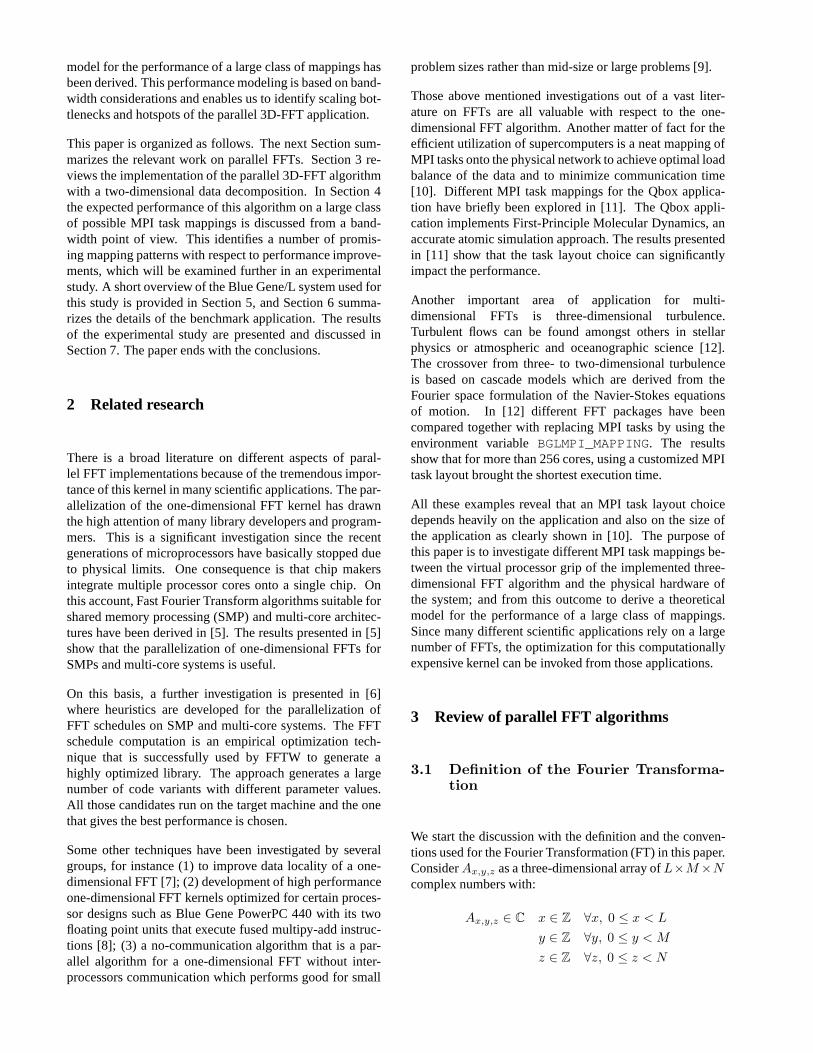
For the three-dimensional case, two different imple-mentations - one-dimensional decomposition and two-dimensional decomposition of the data over the physicalprocessor grid - have been recently investigated [1, 2, 13].The parallel 3D-FFT algorithm using a two-dimensional de-composition is often referred to in the literature as the volu-metric fast Fourier transform. In this paper we concentrateon the performance characteristics of the MPI task place-ments of the two-dimensional decomposition method ontoa mesh communication network. Reference [13] providesan initial investigation. Figure 1 illustrates the paralleliza-tion of the 3D-FFT using a two-dimensional decompositionof the data arrayA of sizeL× M × N . The compute taskshave been organized in a two-dimensional virtual processorgrid with Pc columns andPr rows using the MPI Cartesiangrid topology construct [14]. Each individual physical pro-cessor holds anL/Pr × M/Pc × N sized section ofA inits local memory. The entire 3D-FFT is now performed in 5steps

1. Each processor performsL/Pr × M/Pc one-dimensional FFTs of sizeN

2. An All-to-All communication is performed withineach of the rows - marked in the four main colors -of the virtual processor grid to redistribute the data. Atthe end of the step, each processor holds anL/Pr ×M × N/Pc sized section ofA. These arePr indepen-dent All-to-All communications.

3. Each processor performsL/Pr × N/Pc one-dimensional FFTs of sizeM

4. A second set ofPc independent All-to-All communi-cation is performed, this time within the columns ofthe virtual processor grid. At the end of this step, each

processor holds aL × M/Pc × N/Pr size section ofA.

5. Each processor performsM/Pc × N/Pr one-dimensional FFTs of sizeL

For more information on the parallelization, the reader isreferred to [1, 13].

4 All-to-All transformations on meshed net-work

4.1 Virtual processor grid and physicalprocessor mesh

The key point of this paper is to investigate how the per-formance of the 3D-FFT can be influenced by the choiceof MPI task mapping between the virtual processor gridand the physical processor mesh or torus of the machine.We assume a (partition of the) system of cuboidal shapein 3 dimensions with a physical mesh of processors sizednx × ny × nz. It is absolutely crucial not to confuse thisphysical mesh with the virtual processor grid of dimensionPr × Pc. We denote the total number of processors withPand if we use all processors available for the 3D-FFT, weget

P = nx ny nz = Pr Pc . (2)

If we denote the total amount of data involved in the 3D-FFT byDT and assume this data can be evenly divided ontothe processors, the amount of dataDr held by each row ofthe virtual processor grid becomes

Dr =DT

Pr

= Pc

DT

P. (3)

Each of thePr All-to-All transformations in the second stepof the algorithm needs to redistribute this amount of data. Asimilar equation holds for the second All-to-All transforma-tion in the fourth step.

In the remainder of this section, we discuss how the map-ping of the rows of the virtual processor grid onto the phys-ical processor mesh impacts the interconnect bandwidthavailable to each individual row. Since the map betweenthe virtual grid and the physical mesh has to place all thegrid rows simultaneously and the performance of the worstperforming row will determine the overall performance, werestrict ourselves to maps which obey certain symmetries.The symmetries protect against unequal performance acrossdifferent rows and make it easier to fill the entire physicalmesh of the machine by applying a displaced version of thesame basic map for each of the rows.

perform 1D-FFT

along z-dimension

(a)

perform 1D-FFT

along y-dimension

(b)

Proc 0

Proc 1

Proc 2

Proc 3

Proc 4

Proc 5

Proc 6

Proc 7

Proc 8

Proc 9

Proc 10

Proc 11

Proc 12

Proc 13

Proc 14

Proc 15

All-to-All communication

within the ROWs of the

virtual processor grid

to get data over

y-dimension

locally

perform 1D-FFT

along x-dimension

(c)

All-to-All communication

within the COLUMNs of the

virtual processor grid

to get data over

x-dimension

locally

xz

y

x

z

y

x

zy

data array

A = 8 x 8 x 8

x

z

y

PrPc

2D virtual Processor grid

Pr x Pc = 4 x 4

0

1

2

3

12

3

.

.

.

.

.

.

Figure 1: Computational steps of the 3D-FFT implementationusing 2D-decomposition

i

ni

ni

2

ni

ni

2

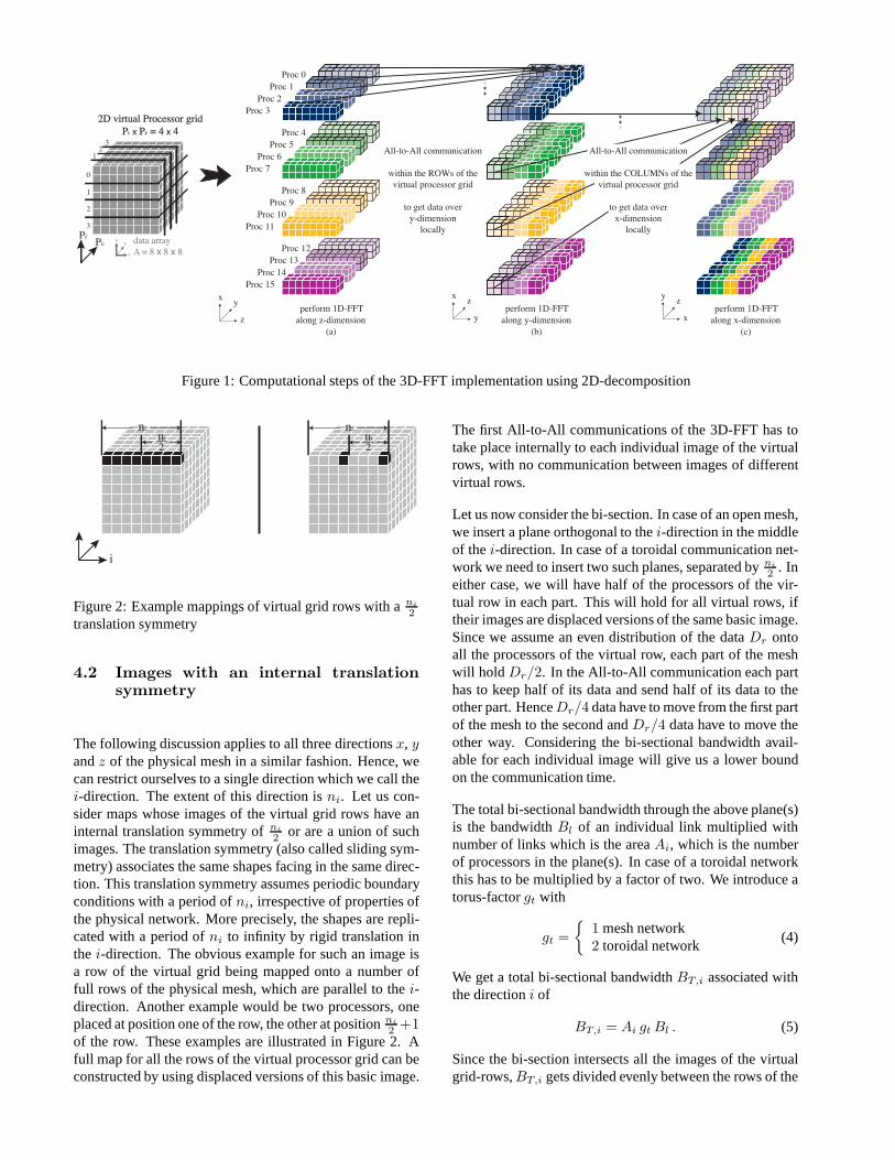
Figure 2: Example mappings of virtual grid rows with ani

2translation symmetry

4.2 Images with an internal translationsymmetry

The following discussion applies to all three directionsx, yandz of the physical mesh in a similar fashion. Hence, wecan restrict ourselves to a single direction which we call thei-direction. The extent of this direction isni. Let us con-sider maps whose images of the virtual grid rows have aninternal translation symmetry ofni

2 or are a union of suchimages. The translation symmetry (also called sliding sym-metry) associates the same shapes facing in the same direc-tion. This translation symmetry assumes periodic boundaryconditions with a period ofni, irrespective of properties ofthe physical network. More precisely, the shapes are repli-cated with a period ofni to infinity by rigid translation inthe i-direction. The obvious example for such an image isa row of the virtual grid being mapped onto a number offull rows of the physical mesh, which are parallel to thei-direction. Another example would be two processors, oneplaced at position one of the row, the other at positionni

2 +1of the row. These examples are illustrated in Figure 2. Afull map for all the rows of the virtual processor grid can beconstructed by using displaced versions of this basic image.

The first All-to-All communications of the 3D-FFT has totake place internally to each individual image of the virtualrows, with no communication between images of differentvirtual rows.

Let us now consider the bi-section. In case of an open mesh,we insert a plane orthogonal to thei-direction in the middleof thei-direction. In case of a toroidal communication net-work we need to insert two such planes, separated byni

2 . Ineither case, we will have half of the processors of the vir-tual row in each part. This will hold for all virtual rows, iftheir images are displaced versions of the same basic image.Since we assume an even distribution of the dataDr ontoall the processors of the virtual row, each part of the meshwill hold Dr/2. In the All-to-All communication each parthas to keep half of its data and send half of its data to theother part. HenceDr/4 data have to move from the first partof the mesh to the second andDr/4 data have to move theother way. Considering the bi-sectional bandwidth avail-able for each individual image will give us a lower boundon the communication time.

The total bi-sectional bandwidth through the above plane(s)is the bandwidthBl of an individual link multiplied withnumber of links which is the areaAi, which is the numberof processors in the plane(s). In case of a toroidal networkthis has to be multiplied by a factor of two. We introduce atorus-factorgt with

gt =

{

1 mesh network2 toroidal network

(4)

We get a total bi-sectional bandwidthBT,i associated withthe directioni of

BT,i = Ai gt Bl . (5)

Since the bi-section intersects all the images of the virtualgrid-rows,BT,i gets divided evenly between the rows of the

i

ni

f

ni

Figure 3: Example mapping of a virtual grid row, with anextent ofni/fi and a translation symmetry ofni/(2fi)

virtual processor grid. For the bandwidthBr,i available foreach individual virtual grid row we get

Br,i =BT,i

Pr

=AigtBl

PPc (6)

From this we get a timet(f)r,i , which is the minimum time

required for the data transfer in thei-direction through thebi-section of

t(f)r,i =

14Dr

Br,i

=DT

4AigtBl

=niDT

4PgtBl

. (7)

The last step usesAini = P .

4.3 Images spanning fractions of direc-tions

We now consider the situation thatfi planes orthogonalto the i-direction are placed inside the physical processormesh, withfi being an integer larger than one. These planesare spaced at regular intervalsni/fi. We assume the basicimage of an individual row of the virtual processor grid canbe placed inside the space between two neighboring planesand has an internal translation symmetry ofni/(2fi) withrespect to a period ofni/fi. This is illustrated in Figure 3.Also here the translation symmetry (or sliding symmetry)involves the same shapes facing in the same direction. Thefull map for all rows is now constructed by using displace-ments of the above basic image across the entire physicalmesh of the hardware.

Assuming efficient message routing along the shortest path,no message will cross any of thefi planes, since this wouldresult in a longer than necessary route. We can thereforeregard the first set of All-to-All transformations within therows of the virtual grid as being executed independently onfi independent machines. Each of thesefi machines has an

extent of its physical mesh of

n′

i =ni

fi

. (8)

The crucial observation is that each of these machines nowholds

D′

T =DT

fi

(9)

data. Since no message crosses any of thefi planes, wealways have an open mesh and

g′t = 1 . (10)

So far we have not split any of the directions orthogonalto the i-direction, which keeps the area of the bi-sectionunchanged

A′

i = Ai . (11)

Inserting everything into a formula similar to equation (7),we obtain

t(p)r,i =

D′

T

4A′

ig′

tBl

=DT

4fiAiBl

=niDT

4fiPBl

. (12)

Again, for the last step, we have usedniAi = P . Whencompared to equation (7), this is an improvement offi/gt.

Obviously this formula will not hold forni = fi, sincethis case does not have an internal translation symmetry ofni/(2fi) = 1/2. For ni = fi all processors belongingto the image of a single row of the virtual grid are within asingle layer of the physical mesh. This layer is orthogonal tothe i-direction. There are no communication requirementsin thei-direction in this case and the associated time is zero

t(1)r,i = 0 . (13)

4.4 Communication time for a given map

After discussing the time constraint associated with the datatransfer in a particular direction for three different symme-try classes, we continue with a discussion of the total com-munication time of the entire parallel 3D-FFT algorithm.The total communication timet is the sum of the timestr and tc for the data exchange within the rows and thecolumns of the virtual processor grid

t = tr + tc . (14)

The timestr andtc can not be shorter than the largest of thetimes required for the data transfer through the bi-sections

tr ≥ maxi

(tr,i) , tc ≥ maxi

(tc,i) . (15)

We restrict the following discussion to maps for which foreach of thetr,i andtc,i either of the equations (7), (12) and(13) can be applied. We now investigate which maps fromthis group are marked out as particularly efficient by our

model. To do so, we rewrite the right hand side of equa-tion (15) as

tr ≥ maxi

(mi)DT

4PBl

(16)

mi =

ni

gt

if equation (7) appliesni

fi

if equation (12) applies

0 if equation (13) applies

A similar equation holds fortc. Themi can be regarded asthe effective length of the image in thei-direction. To op-timize the performance we have to aim to get the largest ofthemi as small as possible. This can typically be achievedby removing holes from the basic row images or by increas-ing themi in either of the other directions. Hence, optimumperformance is obtained if all themi are equally small.

The maps for the rows and the columns are not indepen-dent. The entire 3D-FFT algorithm requires information tobe exchanged through the entire (partition of the) machine.Therefore eithertr or tc can not perform better than thetime t

(f)r,i associated with the longest of theni. By selecting

a good mapping between the virtual processor grid and thephysical mesh we can only improve eithertr or tc but notboth.

We note some important observations on equation (16):

• For a given machine geometrynx, ny, andnz there isno explicit dependency onPc or Pr.

• In the limit of P → ∞ our model agrees with themodel presented in [2] for a single All-to-All trans-formation on a row, plane, or a volume of the physicalmesh of the machine. For finiteP our model giveslonger times.

Our model assumes that all maps are capable of utilizing thefull bandwidthBl of the links at the bi-section at their best.Obviously for very small problems, latency considerations(which do not form part of our model) will dominate.

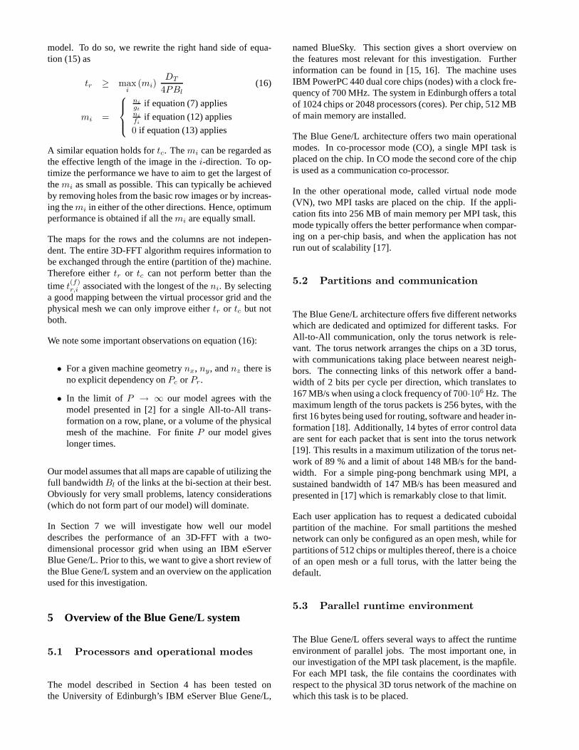
In Section 7 we will investigate how well our modeldescribes the performance of an 3D-FFT with a two-dimensional processor grid when using an IBM eServerBlue Gene/L. Prior to this, we want to give a short review ofthe Blue Gene/L system and an overview on the applicationused for this investigation.

5 Overview of the Blue Gene/L system

5.1 Processors and operational modes

The model described in Section 4 has been tested onthe University of Edinburgh’s IBM eServer Blue Gene/L,

named BlueSky. This section gives a short overview onthe features most relevant for this investigation. Furtherinformation can be found in [15, 16]. The machine usesIBM PowerPC 440 dual core chips (nodes) with a clock fre-quency of 700 MHz. The system in Edinburgh offers a totalof 1024 chips or 2048 processors (cores). Per chip, 512 MBof main memory are installed.

The Blue Gene/L architecture offers two main operationalmodes. In co-processor mode (CO), a single MPI task isplaced on the chip. In CO mode the second core of the chipis used as a communication co-processor.

In the other operational mode, called virtual node mode(VN), two MPI tasks are placed on the chip. If the appli-cation fits into 256 MB of main memory per MPI task, thismode typically offers the better performance when compar-ing on a per-chip basis, and when the application has notrun out of scalability [17].

5.2 Partitions and communication

The Blue Gene/L architecture offers five different networkswhich are dedicated and optimized for different tasks. ForAll-to-All communication, only the torus network is rele-vant. The torus network arranges the chips on a 3D torus,with communications taking place between nearest neigh-bors. The connecting links of this network offer a band-width of 2 bits per cycle per direction, which translates to167 MB/s when using a clock frequency of700·106 Hz. Themaximum length of the torus packets is 256 bytes, with thefirst 16 bytes being used for routing, software and header in-formation [18]. Additionally, 14 bytes of error control dataare sent for each packet that is sent into the torus network[19]. This results in a maximum utilization of the torus net-work of 89 % and a limit of about 148 MB/s for the band-width. For a simple ping-pong benchmark using MPI, asustained bandwidth of 147 MB/s has been measured andpresented in [17] which is remarkably close to that limit.

Each user application has to request a dedicated cuboidalpartition of the machine. For small partitions the meshednetwork can only be configured as an open mesh, while forpartitions of 512 chips or multiples thereof, there is a choiceof an open mesh or a full torus, with the latter being thedefault.

5.3 Parallel runtime environment

The Blue Gene/L offers several ways to affect the runtimeenvironment of parallel jobs. The most important one, inour investigation of the MPI task placement, is the mapfile.For each MPI task, the file contains the coordinates withrespect to the physical 3D torus network of the machine onwhich this task is to be placed.

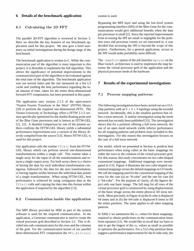
6 Details of the benchmark application

6.1 Calculating the 1D FFT

The parallel 3D-FFT algorithm is reviewed in Section 3.Here we describe the key features of our benchmark ap-plication used for this project. We also give a brief sum-mary on initial investigations during the design stage of thebenchmark.

The benchmark application is written in C. While the com-munication part of the algorithm is most important to thisproject, it is desirable to implement the full algorithm. Thisallows the significance of potential improvements to thecommunication part of the algorithm to be evaluated againstthe total time of the algorithm. The benchmark applicationwas run several times and the one measured on a hot L3cache and yielding the best performance regarding the to-tal amount of time, taken for the entire three-dimensionalforward FFT computation, has been presented in this paper.

The application uses version 2.1.5 of the open-source“Fastest Fourier Transform in the West” (FFTW) library[20] to perform the required one-dimensional FFTs. TheVienna University of Technology offers a FFTW 2.1.5 ver-sion specifically optimized for the double floating point unitof the Blue Gene processors and is known as FFTW-GEL[21, 22]. A detailed comparison by one of the present au-thors confirms the FFTW-GEL library yields a substantialperformance improvement over a version of the library di-rectly compiled from the source [13]. Hence FFTW-GEL isused for this project.

Our application calls the routinefftw() from the FFTW-GEL library which can perform several one-dimensionaltransformations within a single call. This routine takes asingle array for the input of all the transformations and re-turns a single output array. For both arrays there is a choiceof having the data for each individual transformation con-tiguous, followed by the data for the next transformation,or having regular strides between the individual data pointsof a single transformation. When using FFTW-GEL, bestperformance is achieved by using contiguous data in thefftw() -calls and copying the data into this format withinthe application if required by the algorithm [13].

6.2 Communication inside the application

The MPI library provided by IBM as part of the systemsoftware is used for the required communication. In theapplication, a Cartesian communicator is used to create thevirtual processor grid described in Section 3.2. This is di-vided into sub-communicators for the rows and the columnsof the grid. For the communication kernel of our parallelthree-dimensional FFT computation theMPI_Alltoall

routine is used.

Bypassing the MPI layer and using the low-level systemprogramming interface (SPI) of the Blue Gene for the com-munications would give additional benefits when the dataper processor is small [2]. Since the reported improvementsfrom accessing the SPI are small or negligible for the prob-lem sizes and processor counts we are interested in, it wasdecided that accessing the SPI is beyond the scope of thisproject. Furthermore, for a general application, access tothe SPI would make portability more difficult.

The-mapfile option of the job launchermpirun on theBlue Gene/L architecture is used to implement the map be-tween the virtual processor grid of the application and thephysical processor mesh of the hardware.

7 Results of the experimental investigations

7.1 Process mapping patterns

The following investigations have been carried out on a 512-chip partition with an8 × 8 × 8 topology using the toroidalnetwork. Incidentally, this is the smallest partition thatof-fers a torus network. A similar investigation using the meshnetwork has recently been published [13]. The investigationshows that for a partition offering a full torus network, theuse of an open mesh network yields inferior performancefor all mapping patterns and problem sizes included in thisinvestigation. For this reason this investigation focusesonthe case of a full torus network.

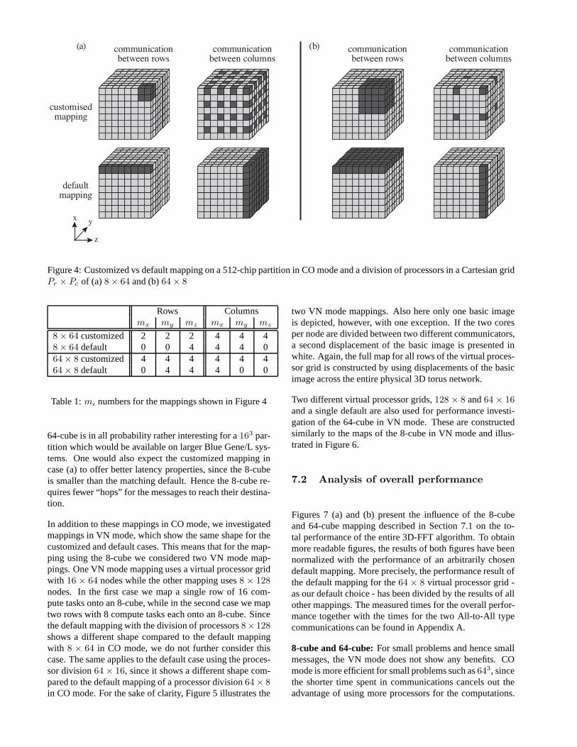
Our model, which we presented in Section 4, predicts bestperformance when using cubes as the basic mappings foreither the rows or the columns of the virtual processor grid.For this reason, this study concentrates on two cube-shapedcustomized mappings. Additional mappings were investi-gated in [13]. Figure 4 illustrates the two cube-shaped cus-tomized mappings versus the default mappings in CO mode.We call the mapping used for the customized mapping of therows for the case (a) an “8-cube” and the one for case (b)a “64-cube”. For the purpose of clarity, all the figures de-pict only one basic image. The full map for all rows of thevirtual processor grid is constructed by using displacementsof the basic image across the entire physical 3D torus net-work. More precisely, in Figure 4 (a) the 8-cube is displaced64 times and in (b) the 64-cube is displaced 8 times to fillthe entire partition. The same applies to all other mappingpatterns.

In Table 1 we summarize themi values for these mappings,required to obtain predictions on the communication timesfrom equation (12). We would like to recall that we have toaim to get the largest of themi values as small as possibleto optimize the performance. For a 512-chip partition thesesuggest a performance improvement for the 8-cube only, the

x y

z

defaultmapping

customisedmapping

communicationbetween rows

communicationbetween columns

communicationbetween rows

communicationbetween columns

(a) (b)

Figure 4: Customized vs default mapping on a 512-chip partition in CO mode and a division of processors in a Cartesian gridPr × Pc of (a)8 × 64 and (b)64 × 8

Rows Columnsmx my mz mx my mz

8 × 64 customized 2 2 2 4 4 48 × 64 default 0 0 4 4 4 064 × 8 customized 4 4 4 4 4 464 × 8 default 0 4 4 4 0 0

Table 1:mi numbers for the mappings shown in Figure 4

64-cube is in all probability rather interesting for a163 par-tition which would be available on larger Blue Gene/L sys-tems. One would also expect the customized mapping incase (a) to offer better latency properties, since the 8-cubeis smaller than the matching default. Hence the 8-cube re-quires fewer “hops” for the messages to reach their destina-tion.

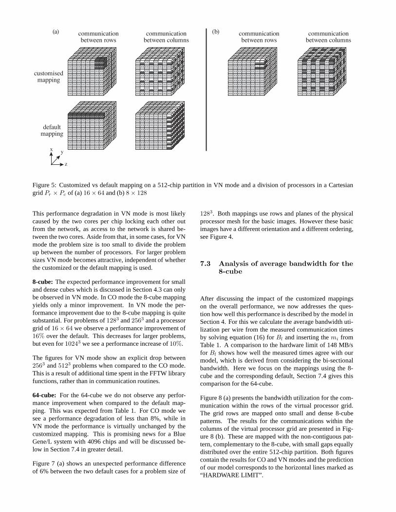
In addition to these mappings in CO mode, we investigatedmappings in VN mode, which show the same shape for thecustomized and default cases. This means that for the map-ping using the 8-cube we considered two VN mode map-pings. One VN mode mapping uses a virtual processor gridwith 16 × 64 nodes while the other mapping uses8 × 128nodes. In the first case we map a single row of 16 com-pute tasks onto an 8-cube, while in the second case we maptwo rows with 8 compute tasks each onto an 8-cube. Sincethe default mapping with the division of processors8× 128shows a different shape compared to the default mappingwith 8 × 64 in CO mode, we do not further consider thiscase. The same applies to the default case using the proces-sor division64 × 16, since it shows a different shape com-pared to the default mapping of a processor division64 × 8in CO mode. For the sake of clarity, Figure 5 illustrates the

two VN mode mappings. Also here only one basic imageis depicted, however, with one exception. If the two coresper node are divided between two different communicators,a second displacement of the basic image is presented inwhite. Again, the full map for all rows of the virtual proces-sor grid is constructed by using displacements of the basicimage across the entire physical 3D torus network.

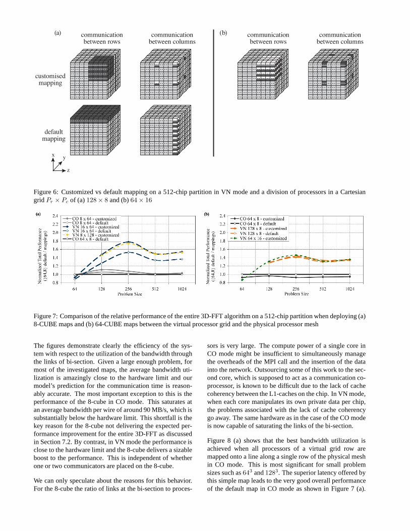
Two different virtual processor grids,128 × 8 and64 × 16and a single default are also used for performance investi-gation of the 64-cube in VN mode. These are constructedsimilarly to the maps of the 8-cube in VN mode and illus-trated in Figure 6.

7.2 Analysis of overall performance

Figures 7 (a) and (b) present the influence of the 8-cubeand 64-cube mapping described in Section 7.1 on the to-tal performance of the entire 3D-FFT algorithm. To obtainmore readable figures, the results of both figures have beennormalized with the performance of an arbitrarily chosendefault mapping. More precisely, the performance result ofthe default mapping for the64 × 8 virtual processor grid -as our default choice - has been divided by the results of allother mappings. The measured times for the overall perfor-mance together with the times for the two All-to-All typecommunications can be found in Appendix A.

8-cube and 64-cube: For small problems and hence smallmessages, the VN mode does not show any benefits. COmode is more efficient for small problems such as643, sincethe shorter time spent in communications cancels out theadvantage of using more processors for the computations.

x y

z

defaultmapping

communicationbetween rows

communicationbetween columns

communicationbetween rows

communicationbetween columns

(a) (b)

customisedmapping

Figure 5: Customized vs default mapping on a 512-chip partition in VN mode and a division of processors in a Cartesiangrid Pr × Pc of (a)16 × 64 and (b)8 × 128

This performance degradation in VN mode is most likelycaused by the two cores per chip locking each other outfrom the network, as access to the network is shared be-tween the two cores. Aside from that, in some cases, for VNmode the problem size is too small to divide the problemup between the number of processors. For larger problemsizes VN mode becomes attractive, independent of whetherthe customized or the default mapping is used.

8-cube: The expected performance improvement for smalland dense cubes which is discussed in Section 4.3 can onlybe observed in VN mode. In CO mode the 8-cube mappingyields only a minor improvement. In VN mode the per-formance improvement due to the 8-cube mapping is quitesubstantial. For problems of1283 and2563 and a processorgrid of 16 × 64 we observe a performance improvement of16% over the default. This decreases for larger problems,but even for10243 we see a performance increase of10%.

The figures for VN mode show an explicit drop between2563 and5123 problems when compared to the CO mode.This is a result of additional time spent in the FFTW libraryfunctions, rather than in communication routines.

64-cube: For the 64-cube we do not observe any perfor-mance improvement when compared to the default map-ping. This was expected from Table 1. For CO mode wesee a performance degradation of less than 8%, while inVN mode the performance is virtually unchanged by thecustomized mapping. This is promising news for a BlueGene/L system with 4096 chips and will be discussed be-low in Section 7.4 in greater detail.

Figure 7 (a) shows an unexpected performance differenceof 6% between the two default cases for a problem size of

1283. Both mappings use rows and planes of the physicalprocessor mesh for the basic images. However these basicimages have a different orientation and a different ordering,see Figure 4.

7.3 Analysis of average bandwidth for the8-cube

After discussing the impact of the customized mappingson the overall performance, we now addresses the ques-tion how well this performance is described by the model inSection 4. For this we calculate the average bandwidth uti-lization per wire from the measured communication timesby solving equation (16) forBl and inserting themi fromTable 1. A comparison to the hardware limit of 148 MB/sfor Bl shows how well the measured times agree with ourmodel, which is derived from considering the bi-sectionalbandwidth. Here we focus on the mappings using the 8-cube and the corresponding default, Section 7.4 gives thiscomparison for the 64-cube.

Figure 8 (a) presents the bandwidth utilization for the com-munication within the rows of the virtual processor grid.The grid rows are mapped onto small and dense 8-cubepatterns. The results for the communications within thecolumns of the virtual processor grid are presented in Fig-ure 8 (b). These are mapped with the non-contiguous pat-tern, complementary to the 8-cube, with small gaps equallydistributed over the entire 512-chip partition. Both figurescontain the results for CO and VN modes and the predictionof our model corresponds to the horizontal lines marked as“HARDWARE LIMIT”.

x y

z

defaultmapping

communicationbetween rows

communicationbetween columns

(a) (b)

customisedmapping

communicationbetween rows

communicationbetween columns

Figure 6: Customized vs default mapping on a 512-chip partition in VN mode and a division of processors in a Cartesiangrid Pr × Pc of (a)128 × 8 and (b)64 × 16

Figure 7: Comparison of the relative performance of the entire 3D-FFT algorithm on a 512-chip partition when deploying (a)8-CUBE maps and (b) 64-CUBE maps between the virtual processor grid and the physical processor mesh

The figures demonstrate clearly the efficiency of the sys-tem with respect to the utilization of the bandwidth throughthe links of bi-section. Given a large enough problem, formost of the investigated maps, the average bandwidth uti-lization is amazingly close to the hardware limit and ourmodel’s prediction for the communication time is reason-ably accurate. The most important exception to this is theperformance of the 8-cube in CO mode. This saturates atan average bandwidth per wire of around 90 MB/s, which issubstantially below the hardware limit. This shortfall is thekey reason for the 8-cube not delivering the expected per-formance improvement for the entire 3D-FFT as discussedin Section 7.2. By contrast, in VN mode the performance isclose to the hardware limit and the 8-cube delivers a sizableboost to the performance. This is independent of whetherone or two communicators are placed on the 8-cube.

We can only speculate about the reasons for this behavior.For the 8-cube the ratio of links at the bi-section to proces-

sors is very large. The compute power of a single core inCO mode might be insufficient to simultaneously managethe overheads of the MPI call and the insertion of the datainto the network. Outsourcing some of this work to the sec-ond core, which is supposed to act as a communication co-processor, is known to be difficult due to the lack of cachecoherency between the L1-caches on the chip. In VN mode,when each core manipulates its own private data per chip,the problems associated with the lack of cache coherencygo away. The same hardware as in the case of the CO modeis now capable of saturating the links of the bi-section.

Figure 8 (a) shows that the best bandwidth utilization isachieved when all processors of a virtual grid row aremapped onto a line along a single row of the physical meshin CO mode. This is most significant for small problemsizes such as643 and1283. The superior latency offered bythis simple map leads to the very good overall performanceof the default map in CO mode as shown in Figure 7 (a).

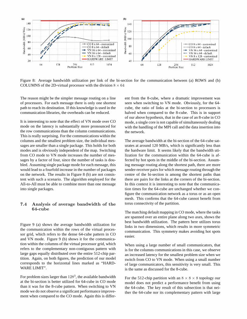
Figure 8: Average bandwidth utilization per link of the bi-section for the communication between (a) ROWS and (b)COLUMNS of the 2D-virtual processor with the division8 × 64

The reason might be the simpler message routing on a lineof processors. For each message there is only one shortestpath to reach its destination. If this knowledge is used in thecommunication libraries, the overheads can be reduced.

It is interesting to note that the effect of VN mode over COmode on the latency is substantially more pronounced forthe row communications than the column communications.This is really surprising. For the communications within thecolumns and the smallest problem size, the individual mes-sages are smaller than a single package. This holds for bothmodes and is obviously independent of the map. Switchingfrom CO mode to VN mode increases the number of mes-sages by a factor of four, since the number of tasks is dou-bled. Assuming single package mode for each message, thiswould lead to a fourfold increase in the number of packageson the network. The results in Figure 8 (b) are not consis-tent with such a scenario. The algorithm employed for theAll-to-All must be able to combine more than one messageinto single packages.

7.4 Analysis of average bandwidth of the64-cube

Figure 9 (a) shows the average bandwidth utilization forthe communication within the rows of the virtual proces-sor grid, which refers to the dense 64-cube pattern in COand VN mode. Figure 9 (b) shows it for the communica-tion within the columns of the virtual processor grid, whichrefers to the complementary non-contiguous pattern withlarge gaps equally distributed over the entire 512-chip par-tition. Again, on both figures, the prediction of our modelcorresponds to the horizontal lines marked as “HARD-WARE LIMIT”.

For problem sizes larger than1283, the available bandwidthat the bi-section is better utilized for 64-cube in CO modethan it was for the 8-cube pattern. When switching to VNmode we do not observe a significant performance improve-ment when compared to the CO mode. Again this is differ-

ent from the 8-cube, where a dramatic improvement wasseen when switching to VN mode. Obviously, for the 64-cube, the ratio of links at the bi-section to processors ishalved when compared to the 8-cube. This is in supportof our above hypothesis, that in the case of an 8-cube in COmode, a single core is not capable of simultaneously dealingwith the handling of the MPI call and the data insertion intothe network.

The average bandwidth at the bi-section of the 64-cube sat-urates at around 120 MB/s, which is significantly less thanthe hardware limit. It seems likely that the bandwidth uti-lization for the communication within the 64-cube is af-fected by hot spots in the middle of the bi-section. Assum-ing message routing along the shortest path, there are moresender-receiver pairs for which message routing through thecentre of the bi-section is among the shortest paths thanthere are pairs for the links at the corners of the bi-section.In this context it is interesting to note that the communica-tion times for the 64-cube are unchanged whether we con-figure the communication network as a torus or as an openmesh. This confirms that the 64-cube cannot benefit fromtorus connectivity of the partition.

The matching default mapping in CO mode, where the tasksare spanned over an entire plane along two axes, shows thebest bandwidth utilization. The pattern here utilizes toruslinks in two dimensions, which results in more symmetriccommunication. This symmetry makes avoiding hot spotseasier.

When using a large number of small communicators, thatis for the columns communications in this case, we observean increased latency for the smallest problem size when weswitch from CO to VN mode. When using a small numberof large communicators, this sensitivity is very small. Thisis the same as discussed for the 8-cube.

For the 512-chip partition with an8 × 8 × 8 topology ourmodel does not predict a performance benefit from usingthe 64-cube. The key result of this subsection is that nei-ther the 64-cube nor its complementary pattern with large

Figure 9: Average bandwidth utilization per link of the bi-section for the communication between (a) ROWS and (b)COLUMNS of the 2D-virtual processor with the division64 × 8

gaps between its processors show severe under-performancewhen compared to the predictions from our model and thematching defaults. This holds for both CO mode and VNmode. The observed decrease in average bandwidth uti-lization is small enough to make the 64-cube an interestingmapping pattern for a larger Blue Gene/L with 4096 chipsin a 16 × 16 × 16 partition. On such a machine one couldhope for improvements similar to the ones we have reportedfor the 8-cube on the 512-chip partition available to us. Ob-viously this needs experimental verification on such a ma-chine.

8 Conclusions

This paper investigates the potential performance benefitfrom MPI task placement for the volumetric Fast FourierTransformation on a modern massively parallel machinewith a meshed or toroidal communication network. Froma detailed discussion of the communication bandwidththrough the bi-section of the communication network, webuild a simple model for the communication times of thealgorithm. The model can be applied to a large number ofMPI mappings between the virtual processor grid of the al-gorithm and the physical mesh of the machine. From theconsidered maps, our model predicts best performance if ei-ther the rows or the columns are mapped onto small cubes.

Our experimental results show also that performance bene-fits of up to 16% for the entire 3D-FFT algorithm are pos-sible when using cubes for the images on a 512-chip par-tition of the machine. The observed performance increaseof the communication part due to task placement is as largeas 33%. This indicates the remaining scope of performanceimprovement due to task placements if the serial part of thealgorithm, such as the deployed FFT routine, would be fur-ther optimized. For small problem sizes, our investigationsdo not show a benefit from using cubes for the images. Thereason for this quite likely lies within the communicationlibrary and its implementation.

Furthermore, our results show that for larger installationsthan were available for this study, the 64-cube pattern lookspromising with respect to performance improvements. Inour investigation this map and its complementary map donot show any critical performance degradation. Obviouslythis needs experimental confirmation on such a larger ma-chine.

Our measurements also show that for small problems, uti-lizing the VN mode which places two computational taskson a dual core chip, is detrimental to the performance of the3D-FFT. This has been traced to a large number of smallcommunicators performing exceptionally well when onlyone of the cores is active. If two cores were active theymight be locking each other out from shared access to thenetwork.

Acknowledgements

We would like to thank Mark Bull (EPCC) for valuablecomments on an earlier version of the manuscript.

A Numerical results of the 3D-FFT computa-tion

The following table gives the total times used by our bench-mark for a forward transformation.

Problem size: 643 1283 2563 5123 10243

CO8×64 cust.: 0.359 ms 2.20 ms 18.9 ms 188 ms 1.78 sCO8×64 def.: 0.356 ms 2.31 ms 19.8 ms 193 ms 1.82 sVN 16×64 cust.: 0.382 ms 1.66 ms 11.4 ms 128 ms 1.21 sVN 16×64 def.: 0.400 ms 1.93 ms 13.3 ms 142 ms 1.34 sVN 8×128 cust.: — 1.68 ms 11.7 ms 128 ms 1.20 sCO64×8 cust.: 0.383 ms 2.54 ms 21.9 ms 203 ms 1.94 sCO64×8 def.: 0.355 ms 2.44 ms 20.3 ms 191 ms 1.84 sVN 128×8 cust.: — 1.89 ms 14.4 ms 147 ms 1.37 sVN 128×8 def.: — 1.91 ms 14.1 ms 143 ms 1.36 sVN 64×16 cust.: 0.410 ms 1.86 ms 13.9 ms 145 ms 1.35 s

Table 2 summarizes the times for the communication withinthe rows of the two-dimensional virtual processor grid usedby our 3D-FFT application.

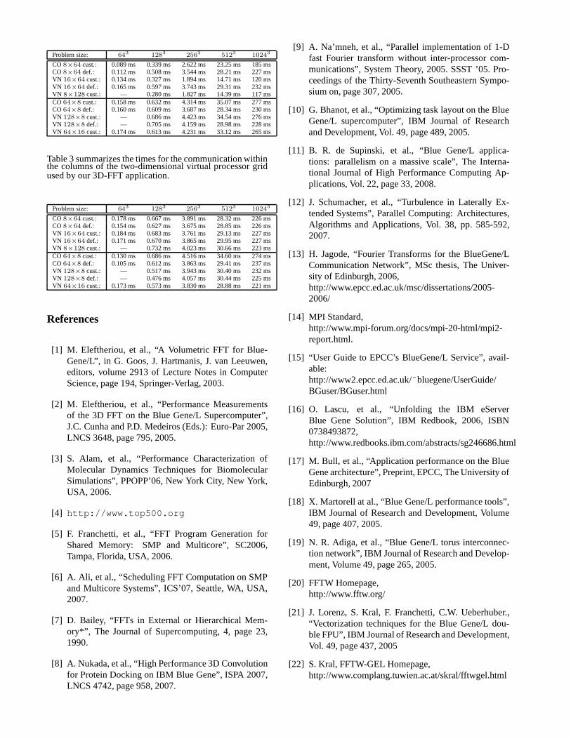
Problem size: 643 1283 2563 5123 10243

CO8×64 cust.: 0.089 ms 0.339 ms 2.622 ms 23.25 ms 185 msCO8×64 def.: 0.112 ms 0.508 ms 3.544 ms 28.21 ms 227 msVN 16×64 cust.: 0.134 ms 0.327 ms 1.894 ms 14.71 ms 120 msVN 16×64 def.: 0.165 ms 0.597 ms 3.743 ms 29.31 ms 232 msVN 8×128 cust.: — 0.280 ms 1.827 ms 14.39 ms 117 msCO64×8 cust.: 0.158 ms 0.632 ms 4.314 ms 35.07 ms 277 msCO64×8 def.: 0.160 ms 0.609 ms 3.687 ms 28.34 ms 230 msVN 128×8 cust.: — 0.686 ms 4.423 ms 34.54 ms 276 msVN 128×8 def.: — 0.705 ms 4.159 ms 28.98 ms 228 msVN 64×16 cust.: 0.174 ms 0.613 ms 4.231 ms 33.12 ms 265 ms

Table 3 summarizes the times for the communication withinthe columns of the two-dimensional virtual processor gridused by our 3D-FFT application.

Problem size: 643 1283 2563 5123 10243

CO8×64 cust.: 0.178 ms 0.667 ms 3.891 ms 28.32 ms 226 msCO8×64 def.: 0.154 ms 0.627 ms 3.675 ms 28.85 ms 226 msVN 16×64 cust.: 0.184 ms 0.683 ms 3.761 ms 29.13 ms 227 msVN 16×64 def.: 0.171 ms 0.670 ms 3.865 ms 29.95 ms 227 msVN 8×128 cust.: — 0.732 ms 4.023 ms 30.66 ms 223 msCO64×8 cust.: 0.130 ms 0.686 ms 4.516 ms 34.60 ms 274 msCO64×8 def.: 0.105 ms 0.612 ms 3.863 ms 29.41 ms 237 msVN 128×8 cust.: — 0.517 ms 3.943 ms 30.40 ms 232 msVN 128×8 def.: — 0.476 ms 4.057 ms 30.44 ms 225 msVN 64×16 cust.: 0.173 ms 0.573 ms 3.830 ms 28.88 ms 221 ms

References

[1] M. Eleftheriou, et al., “A Volumetric FFT for Blue-Gene/L”, in G. Goos, J. Hartmanis, J. van Leeuwen,editors, volume 2913 of Lecture Notes in ComputerScience, page 194, Springer-Verlag, 2003.

[2] M. Eleftheriou, et al., “Performance Measurementsof the 3D FFT on the Blue Gene/L Supercomputer”,J.C. Cunha and P.D. Medeiros (Eds.): Euro-Par 2005,LNCS 3648, page 795, 2005.

[3] S. Alam, et al., “Performance Characterization ofMolecular Dynamics Techniques for BiomolecularSimulations”, PPOPP’06, New York City, New York,USA, 2006.

[4] http://www.top500.org

[5] F. Franchetti, et al., “FFT Program Generation forShared Memory: SMP and Multicore”, SC2006,Tampa, Florida, USA, 2006.

[6] A. Ali, et al., “Scheduling FFT Computation on SMPand Multicore Systems”, ICS’07, Seattle, WA, USA,2007.

[7] D. Bailey, “FFTs in External or Hierarchical Mem-ory*”, The Journal of Supercomputing, 4, page 23,1990.

[8] A. Nukada, et al., “High Performance 3D Convolutionfor Protein Docking on IBM Blue Gene”, ISPA 2007,LNCS 4742, page 958, 2007.

[9] A. Na’mneh, et al., “Parallel implementation of 1-Dfast Fourier transform without inter-processor com-munications”, System Theory, 2005. SSST ’05. Pro-ceedings of the Thirty-Seventh Southeastern Sympo-sium on, page 307, 2005.

[10] G. Bhanot, et al., “Optimizing task layout on the BlueGene/L supercomputer”, IBM Journal of Researchand Development, Vol. 49, page 489, 2005.

[11] B. R. de Supinski, et al., “Blue Gene/L applica-tions: parallelism on a massive scale”, The Interna-tional Journal of High Performance Computing Ap-plications, Vol. 22, page 33, 2008.

[12] J. Schumacher, et al., “Turbulence in Laterally Ex-tended Systems”, Parallel Computing: Architectures,Algorithms and Applications, Vol. 38, pp. 585-592,2007.

[13] H. Jagode, “Fourier Transforms for the BlueGene/LCommunication Network”, MSc thesis, The Univer-sity of Edinburgh, 2006,http://www.epcc.ed.ac.uk/msc/dissertations/2005-2006/

[14] MPI Standard,http://www.mpi-forum.org/docs/mpi-20-html/mpi2-report.html.

[15] “User Guide to EPCC’s BlueGene/L Service”, avail-able:http://www2.epcc.ed.ac.uk/˜ bluegene/UserGuide/BGuser/BGuser.html

[16] O. Lascu, et al., “Unfolding the IBM eServerBlue Gene Solution”, IBM Redbook, 2006, ISBN0738493872,http://www.redbooks.ibm.com/abstracts/sg246686.html

[17] M. Bull, et al., “Application performance on the BlueGene architecture”, Preprint, EPCC, The University ofEdinburgh, 2007

[18] X. Martorell at al., “Blue Gene/L performance tools”,IBM Journal of Research and Development, Volume49, page 407, 2005.

[19] N. R. Adiga, et al., “Blue Gene/L torus interconnec-tion network”, IBM Journal of Research and Develop-ment, Volume 49, page 265, 2005.

[20] FFTW Homepage,http://www.fftw.org/

[21] J. Lorenz, S. Kral, F. Franchetti, C.W. Ueberhuber.,“Vectorization techniques for the Blue Gene/L dou-ble FPU”, IBM Journal of Research and Development,Vol. 49, page 437, 2005

[22] S. Kral, FFTW-GEL Homepage,http://www.complang.tuwien.ac.at/skral/fftwgel.html