Embed Size (px)
Citation preview

Preprint typeset in JHEP style - PAPER VERSION June 2005
TASI Lectures on SolitonsLecture 1: Instantons
David Tong
Department of Applied Mathematics and Theoretical Physics,
Centre for Mathematical Sciences,
Wilberforce Road,
Cambridge, CB3 OBA, UK
Abstract: This is the first in a series of four lectures on the physics of solitons in su-
persymmetric gauge theories. We start here with Yang-Mills instantons, describing the
moduli space of solutions, the ADHM construction, and applications to supersymmetric
gauge theories in various dimensions.

Contents
1. Instantons 2
1.1 The Basics 2
1.1.1 The Instanton Equations 4
1.1.2 Collective Coordinates 5
1.2 The Moduli Space 7
1.2.1 The Moduli Space Metric 9
1.2.2 An Example: A Single Instanton in SU(2) 10
1.3 Fermi Zero Modes 12
1.3.1 Dimension Hopping 13
1.3.2 Instantons and Supersymmetry 13
1.4 The ADHM Construction 16
1.4.1 The Metric on the Higgs Branch 19
1.4.2 Constructing the Solutions 20
1.4.3 Non-Commutative Instantons 24
1.4.4 Examples of Instanton Moduli Spaces 25
1.5 Applications 27
1.5.1 Instantons and the AdS/CFT Correspondence 27
1.5.2 Instanton Particles and the (2, 0) Theory 30
– 1 –
1. Instantons
30 years after the discovery of Yang-Mills instantons [1], they continue to fascinate
both physicists and mathematicians alike. They have lead to new insights into a wide
range of phenomena, from the structure of the Yang-Mills vacuum [2, 3, 4] to the
classification of four-manifolds [5]. One of the most powerful uses of instantons in
recent years is in the analysis of supersymmetric gauge dynamics where they play a
key role in unravelling the plexus of entangled dualities that relates different theories.
The purpose of this lecture is to review the classical properties of instantons, ending
with some applications to the quantum dynamics of supersymmetric gauge theories.
There exist many good reviews on the subject of instantons. The canonical reference
for basics of the subject remains the beautiful lecture by Coleman [6]. More recent
applications to supersymmetric theories are covered in detail in reviews by Shifman
and Vainshtein [7] and by Dorey, Hollowood, Khoze and Mattis [8]. This latter review
describes the ADHM construction of instantons and overlaps with the current lecture.
1.1 The Basics
The starting point for our journey is four-dimensional, pure SU(N) Yang-Mills theory
with action1
S =1
2e2
∫
d4x TrFµνFµν (1.1)
Motivated by the semi-classical evaluation of the path integral, we search for finite
action solutions to the Euclidean equations of motion,
DµFµν = 0 (1.2)
which, in the imaginary time formulation of the theory, have the interpretation of
mediating quantum mechanical tunnelling events.
The requirement of finite action means that the potential Aµ must become pure
gauge as we head towards the boundary r → ∞ of spatial R4,
Aµ → ig−1 ∂µg (1.3)
1Conventions: We pick Hemitian generators T m with Killing form Tr T mT n = 1
2δmn. We write
Aµ = Am
µT m and Fµν = ∂µAν − ∂νAµ − i[Aµ, Aν ]. Adjoint covariant derivatives are DµX = ∂µX −
i[Aµ, X ]. In this section alone we work with Euclidean signature and indices will wander from top
to bottom with impunity; in the following sections we will return to Minkowski space with signature
(+,−,−,−).
– 2 –

with g(x) = eiT (x) ∈ SU(N). In this way, any finite action configuration provides a
map from ∂R4 ∼= S3∞ into the group SU(N). As is well known, such maps are classified
by homotopy theory. Two maps are said to lie in the same homotopy class if they can
be continuously deformed into each other, with different classes labelled by the third
homotopy group,
Π3(SU(N)) ∼= Z (1.4)
The integer k ∈ Z counts how many times the group wraps itself around spatial S3∞
and is known as the Pontryagin number, or second Chern class. We will sometimes
speak simply of the ”charge” k of the instanton. It is measured by the surface integral
k =1
24π2
∫
S3∞
d3Sµ Tr (∂νg)g−1 (∂ρg)g
−1 (∂σg)g−1 ǫµνρσ (1.5)
The charge k splits the space of field configurations into different sectors. Viewing
R4 as a foliation of concentric S3’s, the homotopy classification tells us that we cannot
transform a configuration with non-trivial winding k 6= 0 at infinity into one with trivial
winding on an interior S3 while remaining in the pure gauge ansatz (1.3). Yet, at the
origin, obviously the gauge field must be single valued, independent of the direction
from which we approach. To reconcile these two facts, a configuration with k 6= 0
cannot remain in the pure gauge form (1.3) throughout all of R4: it must have non-
zero action.
An Example: SU(2)
The simplest case to discuss is the gauge group SU(2) since, as a manifold, SU(2) ∼= S3
and it’s almost possible to visualize the fact that Π3(S3) ∼= Z. (Ok, maybe S3 is a bit
of a stretch, but it is possible to visualize Π1(S1) ∼= Z and Π2(S
2) ∼= Z and it’s not
the greatest leap to accept that, in general, Πn(Sn) ∼= Z). Examples of maps in the
different sectors are
• g(0) = 1, the identity map has winding k = 0
• g(1) = (x4 + ixiσi)/r has winding number k = 1. Here i = 1, 2, 3, and the σi are
the Pauli matrices
• g(k) = [g(1)]k has winding number k.
To create a non-trivial configuration in SU(N), we could try to embed the maps above
into a suitable SU(2) subgroup, say the upper left-hand corner of the N × N matrix.
It’s not obvious that if we do this they continue to be a maps with non-trivial winding
– 3 –

since one could envisage that they now have space to slip off. However, it turns out that
this doesn’t happen and the above maps retain their winding number when embedded
in higher rank gauge groups.
1.1.1 The Instanton Equations
We have learnt that the space of configurations splits into different sectors, labelled by
their winding k ∈ Z at infinity. The next question we want to ask is whether solutions
actually exist for different k. Obviously for k = 0 the usual vacuum Aµ = 0 (or gauge
transformations thereof) is a solution. But what about higher winding with k 6= 0?
The first step to constructing solutions is to derive a new set of equations that the
instantons will obey, equations that are first order rather than second order as in (1.2).
The trick for doing this is usually referred to as the Bogomoln’yi bound [9] although,
in the case of instantons, it was actually introduced in the original paper [1]. From
the above considerations, we have seen that any configuration with k 6= 0 must have
some non-zero action. The Bogomoln’yi bound quantifies this. We rewrite the action
by completing the square,
Sinst =1
2e2
∫
d4x TrFµνFµν
=1
4e2
∫
d4x Tr (Fµν ∓ ⋆F µν)2 ± 2Tr Fµν⋆F µν
≥ ± 1
2e2
∫
d4x ∂µ
(
AνFρσ + 2i3AνAρAσ
)
ǫµνρσ (1.6)
where the dual field strength is defined as ⋆Fµν = 12ǫµνρσF
ρσ and, in the final line,
we’ve used the fact that Fµν⋆F µν can be expressed as a total derivative. The final
expression is a surface term which measures some property of the field configuration
on the boundary S3∞. Inserting the asymptotic form Aν → ig−1∂νg into the above
expression and comparing with (1.5), we learn that the action of the instanton in a
topological sector k is bounded by
Sinst ≥8π2
e2|k| (1.7)
with equality if and only if
Fµν = ⋆Fµν (k > 0)
Fµν = −⋆Fµν (k < 0)
Since parity maps k → −k, we can focus on the self-dual equations F = ⋆F . The
Bogomoln’yi argument (which we shall see several more times in later sections) says
– 4 –

that a solution to the self-duality equations must necessarily solve the full equations of
motion since it minimizes the action in a given topological sector. In fact, in the case
of instantons, it’s trivial to see that this is the case since we have
DµFµν = Dµ
⋆F µν = 0 (1.8)
by the Bianchi identity.
1.1.2 Collective Coordinates
So we now know the equations we should be solving to minimize the action. But
do solutions exist? The answer, of course, is yes! Let’s start by giving an example,
before we move on to examine some of its properties, deferring discussion of the general
solutions to the next subsection.
The simplest solution is the k = 1 instanton in SU(2) gauge theory. In singular
gauge, the connection is given by
Aµ =ρ2(x−X)ν
(x−X)2((x−X)2 + ρ2)ηi
µν (gσig−1) (1.9)
The σi, i = 1, 2, 3 are the Pauli matrices and carry the su(2) Lie algebra indices of
Aµ. The ηi are three 4 × 4 anti-self-dual ’t Hooft matrices which intertwine the group
structure of the index i with the spacetime structure of the indices µ, ν. They are given
by
η1 =
0 0 0 −1
0 0 1 0
0 −1 0 0
1 0 0 0
, η2 =
0 0 −1 0
0 0 0 −1
1 0 0 0
0 1 0 0
, η3 =
0 1 0 0
−1 0 0 0
0 0 0 −1
0 0 1 0
(1.10)
It’s a useful exercise to compute the field strength to see how it inherits its self-duality
from the anti-self-duality of the η matrices. To build an anti-self-dual field strength,
we need to simply exchange the η matrices in (1.9) for their self-dual counterparts,
η1 =
0 0 0 1
0 0 1 0
0 −1 0 0
−1 0 0 0
, η2 =
0 0 −1 0
0 0 0 1
1 0 0 0
0 −1 0 0
, η3 =
0 1 0 0
−1 0 0 0
0 0 0 1
0 0 −1 0
(1.11)
For our immediate purposes, the most important feature of the solution (1.9) is that it
is not unique: it contains a number of parameters. In the context of solitons, these are
known as collective coordinates. The solution (1.9) has eight such parameters. They
are of three different types:
– 5 –

i) 4 translations Xµ: The instanton is an object localized in R4, centered around
the point xµ = Xµ.
ii) 1 scale size ρ: The interpretation of ρ as the size of the instanton can be seen by
rescaling x and X in the above solution to demote ρ to an overall constant.
iii) 3 global gauge transformations g ∈ SU(2): This determines how the instanton is
embedded in the gauge group.
At this point it’s worth making several comments about the solution and its collective
coordinates.
• For the k = 1 instanton, each of the collective coordinates described above is a
Goldstone mode, arising because the instanton configuration breaks a symmetry
of the Lagrangian (1.1). In the case of Xµ and g it is clear that the symmetry
is translational invariance and SU(2) gauge invariance respectively. The param-
eter ρ arises from broken conformal invariance. It’s rather common that all the
collective coordinates of a single soliton are Goldstone modes. It’s not true for
higher k.
• The apparent singularity at xµ = Xµ is merely a gauge artifact (hence the name
”singular gauge”). A plot of a gauge invariant quantity, such as the action density,
reveals a smooth solution. The exception is when the instanton shrinks to zero
size ρ→ 0. This singular configuration is known as the small instanton. Despite
its singular nature, it plays an important role in computing the contribution to
correlation functions in supersymmetric theories. The small instanton lies at
finite distance in the space of classical field configurations (in a way which will
be made precise in Section 1.2).
• You may be surprised that we are counting the gauge modes g as physical pa-
rameters of the solution. The key point is that they arise from the global part of
the gauge symmetry, meaning transformations that don’t die off asymptotically.
These are physical symmetries of the system rather than redundancies. In the
early days of studying instantons the 3 gauge modes weren’t included, but it soon
became apparent that many of the nicer mathematical properties of instantons
(for example, hyperKahlerity of the moduli space) require us to include them, as
do certain physical properties (for example, dyonic instantons in five dimensions)
The SU(2) solution (1.9) has 8 collective coordinates. What about SU(N) solutions?
Of course, we should keep the 4 + 1 translational and scale parameters but we would
expect more orientation parameters telling us how the instanton sits in the larger
– 6 –

SU(N) gauge group. How many? Suppose we embed the above SU(2) solution in
the upper left-hand corner of an N × N matrix. We can then rotate this into other
embeddings by acting with SU(N), modulo the stabilizer which leaves the configuration
untouched. We have
SU(N)/S[U(N − 2) × U(2)] (1.12)
where the U(N−2) hits the lower-right-hand corner and doesn’t see our solution, while
the U(2) is included in the denominator since it acts like g in the original solution (1.9)
and we don’t want to overcount. Finally, the notation S[U(p) × U(q)] means that we
lose the overall central U(1) ⊂ U(p) × U(q). The coset space above has dimension
4N − 8. So, within the ansatz (1.9) embedded in SU(N), we see that the k = 1
solution has 4N collective coordinates. In fact, it turns out that this is all of them and
the solution (1.9), suitably embedded, is the most general k = 1 solution in an SU(N)
gauge group. But what about solutions with higher k? To discuss this, it’s useful to
introduce the idea of the moduli space.
1.2 The Moduli Space
We now come to one of the most important concepts of these lectures: the moduli space.
This is defined to be the space of all solutions to F = ⋆F in a given winding sector k
and gauge group SU(N). Let’s denote this space as Ik,N . We will define similar moduli
spaces for the other solitons and much of these lectures will be devoted to understanding
the different roles these moduli spaces play and the relationships between them.
Coordinates on Ik,N are given by the collective coordinates of the solution. We’ve
seen above that the k = 1 solution has 4N collective coordinates or, in other words,
dim(I1,N) = 4N . For higher k, the number of collective coordinates can be determined
by index theorem techniques. I won’t give all the details, but will instead simply tell
you the answer.
dim(Ik,N) = 4kN (1.13)
This has a very simple interpretation. The charge k instanton can be thought of as k
charge 1 instantons, each with its own position, scale, and gauge orientation. When
the instantons are well separated, the solution does indeed look like this. But when
instantons start to overlap, the interpretation of the collective coordinates can become
more subtle.
– 7 –
Strictly speaking, the index theorem which tells us the result (1.13) doesn’t count the
number of collective coordinates, but rather related quantities known as zero modes.
It works as follows. Suppose we have a solution Aµ satisfying F = ⋆F . Then we can
perturb this solution Aµ → Aµ + δAµ and ask how many other solutions are nearby.
We require the perturbation δAµ to satisfy the linearized self-duality equations,
DµδAν −DνδAµ = ǫµνρσDρδAσ (1.14)
where the covariant derivative Dµ is evaluated on the background solution. Solutions
to (1.14) are called zero modes. The idea of zero modes is that if we have the most
general solution Aµ = Aµ(xµ, Xα), where Xα denote all the collective coordinates, then
for each collective coordinate we can define the zero mode δαAµ = ∂Aµ/∂Xα which
will satisfy (1.14). In general however, it is not guaranteed that any zero mode can be
successfully integrated to give a corresponding collective coordinate. But it will turn
out that all the solitons discussed in these lectures do have this property (at least this
is true for bosonic collective coordinates; there is a subtlety with the Grassmannian
collective coordinates arising from fermions which we’ll come to shortly).
Of course, any local gauge transformation will also solve the linearized equations
(1.14) so we require a suitable gauge fixing condition. We’ll write each zero mode to
include an infinitesimal gauge transformation Ωα,
δαAµ =∂Aµ
∂Xα+ DµΩα (1.15)
and choose Ωα so that δαAµ is orthogonal to any other gauge transformation, meaning∫
d4x Tr (δαAµ)Dµη = 0 ∀ η (1.16)
which, integrating by parts, gives us our gauge fixing condition
Dµ (δαAµ) = 0 (1.17)
This gauge fixing condition does not eliminate the collective coordinates arising from
global gauge transformations which, on an operational level, gives perhaps the clearest
reason why we must include them. The Atiyah-Singer index theorem counts the number
of solutions to (1.14) and (1.17) and gives the answer (1.13).
So what does the most general solution, with its 4kN parameters, look like? The
general explicit form of the solution is not known. However, there are rather clever
ansatze which give rise to various subsets of the solutions. Details can be found in the
original literature [10, 11] but, for now, we head in a different, and ultimately more
important, direction and study the geometry of the moduli space.
– 8 –

1.2.1 The Moduli Space Metric
A priori, it is not obvious that Ik,N is a manifold. In fact, it does turn out to be a smooth
space apart from certain localized singularities corresponding to small instantons at
ρ→ 0 where the field configuration itself also becomes singular.
The moduli space Ik,N inherits a natural metric from the field theory, defined by the
overlap of zero modes. In the coordinates Xα, α = 1, . . . , 4kN , the metric is given by
gαβ =1
2e2
∫
d4x Tr (δαAµ) (δβAµ) (1.18)
It’s hard to overstate the importance of this metric. It distills the information contained
in the solutions to F = ⋆F into a more manageable geometric form. It turns out that
for many applications, everything we need to know about the instantons is contained
in the metric gαβ, and this remains true of similar metrics that we will define for other
solitons. Moreover, it is often much simpler to determine the metric (1.18) than it is
to determine the explicit solutions.
The metric has a few rather special properties. Firstly, it inherits certain isometries
from the symmetries of the field theory. For example, both the SO(4) rotation sym-
metry of spacetime and the SU(N) gauge action will descend to give corresponding
isometries of the metric gαβ on Ik,N .
Another important property of the metric (1.18) is that it is hyperKahler, meaning
that the manifold has reduced holonomy Sp(kN) ⊂ SO(4kN). Heuristically, this means
that the manifold admits something akin to a quaternionic structure2. More precisely,
a hyperKahler manifold admits three complex structures J i, i = 1, 2, 3 which obey the
relation
J i J j = −δij + ǫijk Jk (1.19)
The simplest example of a hyperKahler manifold is R4, viewed as the quaternions.
The three complex structures can be taken to be the anti-self-dual ’t Hooft matrices ηi
that we defined in (1.10), each of which gives a different complex pairing of R4. For
example, from η3 we get z1 = x1 + ix2 and z2 = x3 − ix4.
2Warning: there is also something called a quaternionic manifold which arises in N = 2 supergravity
theories [12] and is different from a hyperKahler manifold. For a discussion on the relationship see
[13].
– 9 –

The instanton moduli space Ik,N inherits its complex structures J i from those of R4.
To see this, note if δAµ is a zero mode, then we may immediately write down three
other zero modes ηiνµ δAµ, each of which satisfy the equations (1.14) and (1.17). It
must be possible to express these three new zero modes as a linear combination of the
original ones, allowing us to define three matrices J i,
ηiµν δβAν = (J i)α
β [δαAµ] (1.20)
These matrices J i then descend to three complex structures on the moduli space Ik,N
itself which are given by
(J i)αβ = gαγ
∫
d4x ηiµν Tr δβAµ δγAν (1.21)
So far we have shown only that J i define almost complex structures. To prove hy-
perKahlerity, one must also show integrability which, after some gymnastics, is possible
using the formulae above. A more detailed discussion of the geometry of the moduli
space in this language can be found in [14, 15] and more generally in [16, 17]. For
physicists the simplest proof of hyperKahlerity follows from supersymmetry as we shall
review in section 1.3.
It will prove useful to return briefly to discuss the isometries. In Kahler and hy-
perKahler manifolds, it’s often important to state whether isometries are compatible
with the complex structure J . If the complex structure doesn’t change as we move
along the isometry, so that the Lie derivative LkJ = 0, with k the Killing vector, then
the isometry is said to be holomorphic. In the instanton moduli space Ik,N , the SU(N)
gauge group action is tri-holomorphic, meaning it preserves all three complex struc-
tures. Of the SO(4) ∼= SU(2)L × SU(2)R rotational symmetry, one half, SU(2)L, is
tri-holomorphic, while the three complex structures are rotated under the remaining
SU(2)R symmetry.
1.2.2 An Example: A Single Instanton in SU(2)
In the following subsection we shall show how to derive metrics on Ik,N using the
powerful ADHM technique. But first, to get a flavor for the ideas, let’s take a more
pedestrian route for the simplest case of a k = 1 instanton in SU(2). As we saw above,
there are three types of collective coordinates.
i) The four translational modes are δ(ν)Aµ = ∂Aµ/∂Xν + DµΩν where Ων must be
chosen to satisfy (1.17). Using the fact that ∂/∂Xν = −∂/∂xν , it is simple to
see that the correct choice of gauge is Ων = Aν , so that the zero mode is simply
– 10 –

given by δνAµ = Fµν , which satisfies the gauge fixing condition by virtue of the
original equations of motion (1.2). Computing the overlap of these translational
zero modes then gives
∫
d4x Tr (δ(ν)Aµ δ(ρ)Aµ) = Sinst δνρ (1.22)
ii) One can check that the scale zero mode δAµ = ∂Aµ/∂ρ already satisfies the gauge
fixing condition (1.17) when the solution is taken in singular gauge (1.9). The
overlap integral in this case is simple to perform, yielding
∫
d4x Tr (δAµ δAµ) = 2Sinst (1.23)
iii) Finally, we have the gauge orientations. These are simply of the form δAµ = DµΛ,
but where Λ does not vanish at infinity, so that it corresponds to a global gauge
transformation. In singular gauge it can be checked that the three SU(2) rotations
Λi = [(x−X)2/((x−X)2 + ρ2)]σi satisfy the gauge fixing constraint. These give
rise to an SU(2) ∼= S3 component of the moduli space with radius given by the
norm of any one mode, say, Λ3
∫
d4x Tr (δAµ δAµ) = 2Sinst ρ2 (1.24)
Note that, unlike the others, this component of the metric depends on the collective
coordinate ρ, growing as ρ2. This dependence means that the S3 arising from SU(2)
gauge rotations combines with the R+ from scale transformations to form the space
R4. However, there is a discrete subtlety. Fields in the adjoint representation are left
invariant under the center Z2 ⊂ SU(2), meaning that the gauge rotations give rise to
S3/Z2 rather than S3. Putting all this together, we learn that the moduli space of a
single instanton is
I1,2∼= R4 × R4/Z2 (1.25)
where the first factor corresponds to the position of the instanton, and the second factor
determines its scale size and SU(2) orientation. The normalization of the flat metrics
on the two R4 factors is given by (1.22) and (1.23). In this case, the hyperKahler
structure on I1,2 comes simply by viewing each R4 ∼= H, the quaternions. As is clear
from our derivation, the singularity at the origin of the orbifold R4/Z2 corresponds to
the small instanton ρ→ 0.
– 11 –

1.3 Fermi Zero Modes
So far we’ve only concentrated on the pure Yang-Mills theory (1.1). It is natural
to wonder about the possibility of other fields in the theory: could they also have
non-trivial solutions in the background of an instanton, leading to further collective
coordinates? It turns out that this doesn’t happen for bosonic fields (although they do
have an important impact if they gain a vacuum expectation value as we shall review
in later sections). Importantly, the fermions do contribute zero modes.
Consider a single Weyl fermion λ transforming in the adjoint representation of
SU(N), with kinetic term iTr λ /Dλ. In Euclidean space, we treat λ and λ as inde-
pendent variables, a fact which leads to difficulties in defining a real action. (For the
purposes of this lecture, we simply ignore the issue - a summary of the problem and its
resolutions can be found in [8]). The equations of motion are
/Dλ ≡ σµDµλ = 0 , /Dλ ≡ σµDµλ = 0 (1.26)
where /D = σµDµ and the 2 × 2 matrices are σµ = (σi,−i12). In the background of an
instanton F = ⋆F , only λ picks up zero modes. λ has none. This situation is reversed
in the background of an anti-instanton F = −⋆F . To see that λ has no zero modes in
the background of an instanton, we look at
/D /D = σµσνDµDν = D2 12 + F µν ηiµνσ
i (1.27)
where ηi are the anti-self-dual ’t Hooft matrices defined in (1.10). But a self-dual matrix
Fµν contracted with an anti-self-dual matrix ηµν vanishes, leaving us with /D /D = D2.
And the positive definite operator D2 has no zero modes. In contrast, if we try to
repeat the calculation for λ, we find
/D /D = D2 12 + F µνηiµνσ
i (1.28)
where ηi are the self-dual ’t Hooft matrices (1.11). Since we cannot express the operator
/D /D as a total square, there’s a chance that it has zero modes. The index theorem tells
us that each Weyl fermion λ picks up 4kN zero modes in the background of a charge k
instanton. There are corresponding Grassmann collective coordinates, which we shall
denote as χ, associated to the most general solution for the gauge field and fermions.
But these Grassmann collective coordinates occasionally have subtle properties. The
quick way to understand this is in terms of supersymmetry. And often the quick way
to understand the full power of supersymmetry is to think in higher dimensions.
– 12 –

1.3.1 Dimension Hopping
It will prove useful to take a quick break in order to make a few simple remarks about
instantons in higher dimensions. So far we’ve concentrated on solutions to the self-
duality equations in four-dimensional theories, which are objects localized in Euclidean
spacetime. However, it is a simple matter to embed the solutions in higher dimensions
simply by insisting that all fields are independent of the new coordinates. For example,
in d = 4 + 1 dimensional theories one can set ∂0 = A0 = 0, with the spatial part
of the gauge field satisfying F = ⋆F . Such configurations have finite energy and the
interpretation of particle like solitons. We shall describe some of their properties when
we come to applications. Similarly, in d = 5 + 1, the instantons are string like objects,
while in d = 9 + 1, instantons are five-branes. While this isn’t a particularly deep
insight, it’s a useful trick to keep in mind when considering the fermionic zero modes
of the soliton in supersymmetric theories as we shall discuss shortly.
When solitons have a finite dimensional worldvolume, we can promote the collective
coordinates to fields which depend on the worldvolume directions. These correspond
to massless excitations living on the solitons. For example, allowing the translational
modes to vary along the instanton string simply corresponds to waves propagating along
the string. Again, this simple observation will become rather powerful when viewed in
the context of supersymmetric theories.
A note on terminology: Originally the term ”instanton” referred to solutions to
the self-dual Yang-Mills equations F = ⋆F . (At least this was true once Physical
Review lifted its censorship of the term!). However, when working with theories in
spacetime dimensions other than four, people often refer to the relevant finite action
configuration as an instanton. For example, kinks in quantum mechanics are called
instantons. Usually this doesn’t lead to any ambiguity but in this review we’ll consider
a variety of solitons in a variety of dimensions. I’ll try to keep the phrase“instanton”
to refer to (anti)-self-dual Yang-Mills instantons.
1.3.2 Instantons and Supersymmetry
Instantons share an intimate relationship with supersymmetry. Let’s consider an in-
stanton in a d = 3 + 1 supersymmetric theory which could be either N = 1, N = 2
or N = 4 super Yang-Mills. The supersymmetry transformation for any adjoint Weyl
fermion takes the form
δλ = F µνσµσνǫ , δλ = F µν σµσν ǫ (1.29)
where, again, we treat the infinitesimal supersymmetry parameters ǫ and ǫ as inde-
pendent. But we’ve seen above that in the background of a self-dual solution F = ⋆F
– 13 –
the combination F µν σµσν = 0. This means that the instanton is annihilated by half of
the supersymmetry transformations ǫ, while the other half, ǫ, turn on the fermions λ.
We say that the supersymmetries arising from ǫ are broken by the soliton, while those
arising from ǫ are preserved. Configurations in supersymmetric theories which are an-
nihilated by some fraction of the supersymmetries are known as BPS states (although
the term Witten-Olive state would be more appropriate [18]).
Both the broken and preserved supersymmetries play an important role for solitons.
The broken ones are the simplest to describe, for they generate fermion zero modes
λ = F µνσµσνǫ. These ”Goldstino” modes are a subset of the 4kN fermion zero modes
that exist for each Weyl fermion λ. Further modes can also be generated by acting on
the instanton with superconformal transformations.
The unbroken supersymmetries ǫ play a more important role: they descend to a
supersymmetry on the soliton worldvolume, pairing up bosonic collective coordinates
X with Grassmannian collective coordinates χ. There’s nothing surprising here. It’s
simply the statement that if a symmetry is preserved in a vacuum (where, in this
case, the ”vacuum” is the soliton itself) then all excitations above the vacuum fall
into representations of this symmetry. However, since supersymmetry in d = 0 + 0
dimensions is a little subtle, and the concept of ”excitations above the vacuum” in
d = 0 + 0 dimensions even more so, this is one of the places where it will pay to lift
the instantons to higher dimensional objects. For example, instantons in theories with
8 supercharges (equivalent to N = 2 in four dimensions) can be lifted to instanton
strings in six dimensions, which is the maximum dimension in which Yang-Mills theory
with eight supercharges exists. Similarly, instantons in theories with 16 supercharges
(equivalent to N = 4 in four dimensions) can be lifted to instanton five-branes in ten
dimensions. Instantons in N = 1 theories are stuck in their four-dimensional world.
Considering Yang-Mills instantons as solitons in higher dimensions allows us to see
this relationship between bosonic and fermionic collective coordinates. Consider excit-
ing a long-wavelength mode of the soliton in which a bosonic collective coordinate X
depends on the worldvolume coordinate of the instanton s, so X = X(s). Then if we
hit this configuration with the unbroken supersymmetry ǫ, it will no longer annihilate
the configuration, but will turn on a fermionic mode proportional to ∂sX. Similarly,
any fermionic excitation will be related to a bosonic excitation.
The observation that the unbroken supersymmetries descend to supersymmetries on
the worldvolume of the soliton saves us a lot of work in analyzing fermionic zero modes:
if we understand the bosonic collective coordinates and the preserved supersymmetry,
– 14 –

then the fermionic modes pretty much come for free. This includes some rather subtle
interaction terms.
For example, consider instanton five-branes in ten-dimensional super Yang-Mills.
The worldvolume theory must preserve 8 of the 16 supercharges. The only such theory
in 5 + 1 dimensions is a sigma-model on a hyperKahler target space [19] which, for
instantons, is the manifold Ik,N . The Lagrangian is
L = gαβ∂Xα∂Xβ + iχαDαβχ
β + 14Rαβγδχ
αχβχγχδ (1.30)
where ∂ denotes derivatives along the soliton worldvolume and the covariant derivative
is Dαβ = gαβ∂ + Γγαβ(∂Xγ). This is the slick proof that the instanton moduli space
metric must be hyperKahler: it is dictated by the 8 preserved supercharges.
The final four-fermi term couples the fermionic collective coordinates to the Riemann
tensor. Suppose we now want to go back down to instantons in four dimensional N = 4
super Yang-Mills. We can simply dimensionally reduce the above action. Since there
are no longer worldvolume directions for the instantons, the first two terms vanish, but
we’re left with the term
Sinst = 14Rαβγδχ
αχβχγχδ (1.31)
This term reflects the point we made earlier: zero modes cannot necessarily be lifted
to collective coordinates. Here we see this phenomenon for fermionic zero modes.
Although each such mode doesn’t change the action of the instanton, if we turn on four
Grassmannian collective coordinates at the same time then the action does increase!
One can derive this term without recourse to supersymmetry but it’s a bit of a pain
[20]. The term is very important in applications of instantons.
Instantons in four-dimensional N = 2 theories can be lifted to instanton strings in
six dimensions. The worldvolume theory must preserve half of the 8 supercharges.
There are two such super-algebras in two dimensions, a non-chiral (2, 2) theory and a
chiral (0, 4) theory, where the two entries correspond to left and right moving fermions
respectively. By analyzing the fermionic zero modes one can show that the instanton
string preserves (0, 4) supersymmetry. The corresponding sigma-model doesn’t contain
the term (1.31). (Basically because the χ zero modes are missing). However, similar
terms can be generated if we also consider fermions in the fundamental representation.
Finally, instantons in N = 1 super Yang-Mills preserve (0, 2) supersymmetry on their
worldvolume.
– 15 –

In the following sections, we shall pay scant attention to the fermionic zero modes,
simply stating the fraction of supersymmetry that is preserved in different theories. In
many cases this is sufficient to fix the fermions completely: the beauty of supersymme-
try is that we rarely have to talk about fermions!
1.4 The ADHM Construction
In this section we describe a powerful method to solve the self-dual Yang-Mills equa-
tions F = ⋆F due to Atiyah, Drinfeld, Hitchin and Manin and known as the ADHM
construction [21]. This will also give us a new way to understand the moduli space Ik,N
and its metric. The natural place to view the ADHM construction is twistor space.
But, for a physicist, the simplest place to view the ADHM construction is type II string
theory [22, 23, 24]. We’ll do things the simple way.
The brane construction is another place
N coincident Dp−branes
k D(p−4)−branes
Figure 1: Dp-branes as instantons.
where it’s useful to consider Yang-Mills instan-
tons embedded as solitons in a p+ 1 dimensional
theory with p ≥ 3. With this in mind, let’s
consider a configuration of N Dp-branes, with k
D(p−4)-branes in type II string theory (Type IIB
for p odd; type IIA for p even). A typical con-
figuration is drawn in figure 1. We place all N
Dp-branes on top of each other so that, at low en-
ergies, their worldvolume dynamics is described
by
d = p+ 1 U(N) Super Yang-Mills with 16 Supercharges
For example, if p = 3 we have the familiar N = 4 theory in d = 3 + 1 dimensions. The
worldvolume theory of the Dp-branes also includes couplings to the various RR-fields
in the bulk. This includes the term
Tr
∫
Dp
dp+1x Cp−3 ∧ F ∧ F (1.32)
where F is the U(N) gauge field, and Cp−3 is the RR-form that couples to D(p − 4)-
branes. The importance of this term lies in the fact that it relates instantons on the
Dp-branes to D(p− 4) branes. To see this, note that an instanton with non-zero F ∧Fgives rise to a source (8π2/e2)
∫
dp−3x Cp−3 for the RR-form. This is the same source
induced by a D(p− 4)-brane. If you’re careful in comparing the factors of 2 and π and
such like, it’s not hard to show that the instanton has precisely the mass and charge of
– 16 –

the D(p− 4)-brane [25, 26]. They are the same object! We have the important result
that
Instanton in Dp-Brane ≡ D(p− 4)-Brane (1.33)
The strategy to derive the ADHM construction from branes is to view this whole story
from the perspective of the D(p − 4)-branes [22, 23, 24]. For definiteness, let’s revert
back to p = 3, so that we’re considering D-instantons interacting with D3-branes. This
means that we have to write down the d = 0+0 dimensional theory on the D-instantons.
Since supersymmetric theories in no dimensions may not be very familiar, it will help
to keep in mind that the whole thing can be lifted to higher p.
Suppose firstly that we don’t have the D3-branes. The theory on the D-instantons in
flat space is simply the dimensional reduction of d = 3+1 N = 4 U(k) super Yang-Mills
to zero dimensions. We will focus on the bosonic sector, with the fermions dictated
by supersymmetry as explained in the previous section. We have 10 scalar fields, each
of which is a k × k Hermitian matrix. For later convenience, we split them into two
batches:
(Xµ, Xm) µ = 1, 2, 3, 4; m = 5, . . . , 10 (1.34)
where we’ve put hats on directions transverse to the D3-brane. We’ll use the index
notation (Xµ)αβ to denote the fact that each of these is a k× k matrix. Note that this
is a slight abuse of notation since, in the previous section, α = 1, . . . , 4k rather than
1, . . . , k here. We’ll also introduce the complex notation
Z = X1 + iX2 , W = X3 − iX4 (1.35)
When Xµ and Xm are all mutually commuting, their 10k eigenvalues have the inter-
pretation of the positions of the k D-instantons in flat ten-dimensional space.
What effect does the presence of the D3-branes have? The answer is well known.
Firstly, they reduce the supersymmetry on the lower dimensional brane by half, to
eight supercharges (equivalent to N = 2 in d = 3 + 1). The decomposition (1.34)
reflects this, with the Xm lying in a vector multiplet and the Xµ forming an adjoint
hypermultiplet. The new fields which reduce the supersymmetry areN hypermultiplets,
arising from quantizing strings stretched between the Dp-branes and D(p− 4)-branes.
Each hypermultiplet carries an α = 1, . . . k index, corresponding to the D(p− 4)-brane
on which the string ends, and an a = 1, . . . , N index corresponding to the Dp-brane on
which the other end of the string sits.. Again we ignore fermions. The two complex
scalars in each hypermultiplet are denoted
ψαa , ψa
α (1.36)
– 17 –
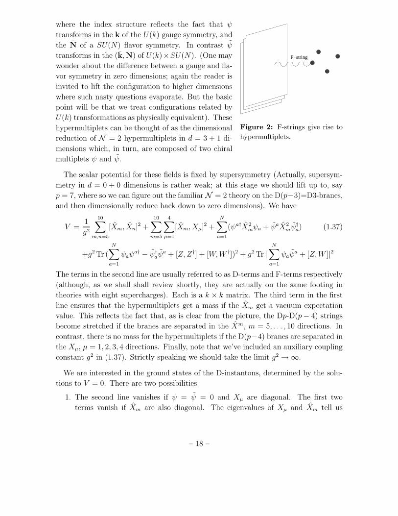
where the index structure reflects the fact that ψ
F−string
Figure 2: F-strings give rise to
hypermultiplets.
transforms in the k of the U(k) gauge symmetry, and
the N of a SU(N) flavor symmetry. In contrast ψ
transforms in the (k,N) of U(k)×SU(N). (One may
wonder about the difference between a gauge and fla-
vor symmetry in zero dimensions; again the reader is
invited to lift the configuration to higher dimensions
where such nasty questions evaporate. But the basic
point will be that we treat configurations related by
U(k) transformations as physically equivalent). These
hypermultiplets can be thought of as the dimensional
reduction of N = 2 hypermultiplets in d = 3 + 1 di-
mensions which, in turn, are composed of two chiral
multiplets ψ and ψ.
The scalar potential for these fields is fixed by supersymmetry (Actually, supersym-
metry in d = 0 + 0 dimensions is rather weak; at this stage we should lift up to, say
p = 7, where so we can figure out the familiar N = 2 theory on the D(p−3)=D3-branes,
and then dimensionally reduce back down to zero dimensions). We have
V =1
g2
10∑
m,n=5
[Xm, Xn]2 +
10∑
m=5
4∑
µ=1
[Xm, Xµ]2 +
N∑
a=1
(ψa†X2mψa + ψaX2
mψ†a) (1.37)
+g2 Tr (
N∑
a=1
ψaψa† − ψ†
aψa + [Z,Z†] + [W,W †])2 + g2 Tr |
N∑
a=1
ψaψa + [Z,W ]|2
The terms in the second line are usually referred to as D-terms and F-terms respectively
(although, as we shall shall review shortly, they are actually on the same footing in
theories with eight supercharges). Each is a k × k matrix. The third term in the first
line ensures that the hypermultiplets get a mass if the Xm get a vacuum expectation
value. This reflects the fact that, as is clear from the picture, the Dp-D(p− 4) strings
become stretched if the branes are separated in the Xm, m = 5, . . . , 10 directions. In
contrast, there is no mass for the hypermultiplets if the D(p−4) branes are separated in
the Xµ, µ = 1, 2, 3, 4 directions. Finally, note that we’ve included an auxiliary coupling
constant g2 in (1.37). Strictly speaking we should take the limit g2 → ∞.
We are interested in the ground states of the D-instantons, determined by the solu-
tions to V = 0. There are two possibilities
1. The second line vanishes if ψ = ψ = 0 and Xµ are diagonal. The first two
terms vanish if Xm are also diagonal. The eigenvalues of Xµ and Xm tell us
– 18 –
where the k D-instantons are placed in flat space. They are unaffected by the
existence of the D3-branes whose presence is only felt at the one-loop level when
the hypermultiplets are integrated out. This is known as the ”Coulomb branch”,
a name inherited from the structure of gauge symmetry breaking: U(k) → U(1)k.
(The name is, of course, more appropriate in dimensions higher than zero where
particles charged under U(1)k experience a Coulomb interaction).
2. The first line vanishes if Xm = 0, m = 5, . . . , 10. This corresponds to the D(p−4)
branes lying on top of the Dp-branes. The remaining fields ψ, ψ, Z and W are
constrained by the second line in (1.37). Since these solutions allow ψ, ψ 6= 0 we
will generically have the U(k) gauge group broken completely, giving the name
”Higgs branch” to this class of solutions. More precisely, the Higgs branch is
defined to be the space of solutions
MHiggs∼= Xm = 0, V = 0/U(k) (1.38)
where we divide out by U(k) gauge transformations. The Higgs branch describes
the D(p−4) branes nestling inside the larger Dp-branes. But this is exactly where
they appear as instantons. So we might expect that the Higgs branch knows
something about this. Let’s start by computing its dimension. We have 4kN
real degrees of freedom in ψ and ψ and a further 4k2 in Z and W . The D-term
imposes k2 real constraints, while the F-term imposes k2 complex constraints.
Finally we lose a further k2 degrees of freedom when dividing by U(k) gauge
transformations. Adding, subtracting, we have
dim(MHiggs) = 4kN (1.39)
which should look familiar (1.13). The first claim of the ADHM construction is that
we have an isomorphism between manifolds,
MHiggs∼= Ik,N (1.40)
1.4.1 The Metric on the Higgs Branch
To summarize, the D-brane construction has lead us to identify the instanton moduli
space Ik,N with the Higgs branch of a gauge theory with 8 supercharges (equivalent to
N = 2 in d = 3 + 1). The field content of this gauge theory is
U(k) Gauge Theory + Adjoint Hypermultiplet Z,W
+ N Fundamental Hypermultiplets ψa, ψa (1.41)
– 19 –

This auxiliary U(k) gauge theory defines its own metric on the Higgs branch. This
metric arises in the following manner: we start with the flat metric on R4k(N+k), pa-
rameterized by ψ, ψ, Z and W . Schematically,
ds2 = |dψ|2 + |dψ|2 + |dZ|2 + |dW |2 (1.42)
This metric looks somewhat more natural if we consider higher dimensional D-branes
where it arises from the canonical kinetic terms for the hypermultiplets. We now pull
back this metric to the hypersurface V = 0, and subsequently quotient by the U(k)
gauge symmetry, meaning that we only consider tangent vectors to V = 0 that are
orthogonal to the U(k) action. This procedure defines a metric on MHiggs. The second
important result of the ADHM construction is that this metric coincides with the one
defined in terms of solitons in (1.18).
I haven’t included a proof of the equivalence between the metrics here, although
it’s not too hard to show (for example, using Maciocia’s hyperKahler potential [17] as
reviewed in [8]). However, we will take time to show that the isometries of the metrics
defined in these two different ways coincide. From the perspective of the auxiliary
U(k) gauge theory, all isometries appear as flavor symmetries. We have the SU(N)
flavor symmetry rotating the hypermultiplets; this is identified with the SU(N) gauge
symmetry in four dimensions. The theory also contains an SU(2)R R-symmetry, in
which (ψ, ψ†) and (Z,W †) both transform as doublets (this will become more apparent
in the following section in equation (1.44)). This coincides with the SU(2)R ⊂ SO(4)
rotational symmetry in four dimensions. Finally, there exists an independent SU(2)L
symmetry rotating just the Xµ.
The method described above for constructing hyperKahler metrics is an example of a
technique known as the hyperKahler quotient [27]. As we have seen, it arises naturally
in gauge theories with 8 supercharges. The D- and F-terms of the potential (1.37) give
what are called the triplet of ”moment-maps” for the U(k) action.
1.4.2 Constructing the Solutions
As presented so far, the ADHM construction relates the moduli space of instantons
Ik,N to the Higgs branch of an auxiliary gauge theory. In fact, we’ve omitted the
most impressive part of the story: the construction can also be used to give solutions
to the self-duality equations. What’s more, it’s really very easy! Just a question of
multiplying a few matrices together. Let’s see how it works.
– 20 –

Firstly, we need to rewrite the vacuum conditions in a more symmetric fashion.
Define
ωa =
(
ψαa
ψ†αa
)
(1.43)
Then the real D-term and complex F-term which lie in the second line of (1.37) and
define the Higgs branch can be combined in to the triplet of constraints,
N∑
a=1
ω†aσ
i ωa − i[Xµ, Xµ]ηiµν = 0 (1.44)
where σi are, as usual, the Pauli matrices and ηi the ’t Hooft matrices (1.10). These
give three k × k matrix equations. The magic of the ADHM construction is that for
each solution to the algebraic equations (1.44), we can build a solution to the set of non-
linear partial differential equations F = ⋆F . Moreover, solutions to (1.44) related by
U(k) gauge transformations give rise to the same field configuration in four dimensions.
Let’s see how this remarkable result is achieved.
The first step is to build the (N + 2k) × 2k matrix ∆,
∆ =
(
ωT
Xµσµ
)
+
(
0
xµσµ
)
(1.45)
where σµ = (σi,−i12). These have the important property that σ[µσν] is self-dual, while
σ[µσν] is anti-self-dual, facts that we also used in Section 1.3 when discussing fermions.
In the second matrix we’ve re-introduced the spacetime coordinate xµ which, here, is
to be thought of as multiplying the k × k unit matrix. Before proceeding, we need a
quick lemma:
Lemma: ∆†∆ = f−1 ⊗ 12
where f is a k × k matrix, and 12 is the unit 2 × 2 matrix. In other words, ∆†∆
factorizes and is invertible.
Proof: Expanding out, we have (suppressing the various indices)
∆†∆ = ω†ω +X†X + (X†x+ x†X) + x†x1k (1.46)
Since the factorization happens for all x ≡ xµσµ, we can look at three terms separately.
The last is x†x = xµσµxνσ
ν = x2 12. So that works. For the term linear in x, we simply
– 21 –

need the fact that Xµ = X†µ to see that it works. What’s more tricky is the term that
doesn’t depend on x. This is where the triplet of D-terms (1.44) comes in. Let’s write
the relevant term from (1.46) with all the indices, including an m,n = 1, 2 index to
denote the two components we introduced in (1.43). We require
ω†αma ωaβn + (Xµ)
αγ(Xν)
γβ σ
µ mpσνpn ∼ δm
n (1.47)
⇔ tr2 σi[
ωω† +X†X]
= 0 i = 1, 2, 3
⇔ ω†σiω +XµXν σµσiσν = 0
But, using the identity σµσiσν = 2iηiµν , we see that this last condition is implied by
the vanishing of the D-terms (1.44). This concludes our proof of the lemma.
The rest is now plain sailing. Consider the matrix ∆ as defining 2k linearly indepen-
dent vectors in CN+2k. We define U to be the (N + 2k) ×N matrix containing the N
normalized, orthogonal vectors. i.e
∆†U = 0 , U †U = 1N (1.48)
Then the potential for a charge k instanton in SU(N) gauge theory is given by
Aµ = iU † ∂µU (1.49)
Note firstly that if U were an N×N matrix, this would be pure gauge. But it’s not, and
it’s not. Note also that Aµ is left unchanged by auxiliary U(k) gauge transformations.
We need to show that Aµ so defined gives rise to a self-dual field strength with winding
number k. We’ll do the former, but the latter isn’t hard either: it just requires more
matrix multiplication. To help us in this, it will be useful to construct the projection
operator P = UU † and notice that this can also be written as P = 1 − ∆f∆†. To see
that these expressions indeed coincide, we can check that PU = U and P∆ = 0 for
both. Now we’re almost there:
Fµν = ∂[µAν] − iA[µAν]
= ∂[µ iU†∂ν]U + iU †(∂[µU)U †(∂ν]U)
= i(∂[µU†)(∂ν]U) − i(∂[µU
†)UU †(∂ν]U)
= i(∂[µU†)(1 − UU †)(∂ν]U)
= i(∂[µU†)∆ f ∆†(∂ν]U)
= iU †(∂[µ∆) f (∂ν]U)
= iU †σ[µfσν]U
– 22 –

At this point we use our lemma. Because ∆†∆ factorizes, we may commute f past σµ.
And that’s it! We can then write
Fµν = iU †fσ[µσν]U = ⋆Fµν (1.50)
since, as we mentioned above, σµν = σ[µσν] is self-dual. Nice huh! What’s harder to
show is that the ADHM construction gives all solutions to the self-dualily equations.
Counting parameters, we see that we have the right number and it turns out that we
can indeed get all solutions in this manner.
The construction described above was first described in ADHM’s original paper,
which weighs in at a whopping 2 pages. Elaborations and extensions to include, among
other things, SO(N) and Sp(N) gauge groups, fermionic zero modes, supersymmetry
and constrained instantons, can be found in [28, 29, 30, 31].
An Example: The Single SU(2) Instanton Revisited
Let’s see how to re-derive the k = 1 SU(2) solution (1.9) from the ADHM method.
We’ll set Xµ = 0 to get a solution centered around the origin. We then have the 4 × 2
matrix
∆ =
(
ωT
xµσµ
)
(1.51)
where the D-term constraints (1.44) tell us that ω†am(σi)m
nωnb = 0. We can use our
SU(2) flavor rotation, acting on the indices a, b = 1, 2, to choose the solution
ω†amω
mb = ρ2δa
b (1.52)
in which case the matrix ∆ becomes ∆T = (ρ12, xµσµ). Then solving for the normalized
zero eigenvectors ∆†U = 0, and U †U = 1, we have
U =
(√
x2/(x2 + ρ2) 12
−√
ρ2/x2(x2 + ρ2) xµσµ
)
(1.53)
From which we calculate
Aµ = iU †∂µU =ρ2xν
x2(x2 + ρ2)ηi
µν σi (1.54)
which is indeed the solution (1.9) as promised.
– 23 –

1.4.3 Non-Commutative Instantons
There’s an interesting deformation of the ADHM construction arising from studying
instantons on a non-commutative space, defined by
[xµ, xν ] = iθµν (1.55)
The most simple realization of this deformation arises by considering functions on the
space R4θ, with multiplication given by the ⋆-product
f(x) ⋆ g(x) = exp
(
i
2θµν
∂
∂yµ
∂
∂xν
)
f(y)g(x)
∣
∣
∣
∣
x=y
(1.56)
so that we indeed recover the commutator xµ ⋆ xν − xν ⋆ xµ = iθµν . To define gauge
theories on such a non-commutative space, one must extend the gauge symmetry from
SU(N) to U(N). When studying instantons, it is also useful to decompose the non-
commutivity parameter into self-dual and anti-self-dual pieces:
θµν = ξi ηiµν + ζ i ηi
µν (1.57)
where ηi and ηi are defined in (1.11) and (1.10) respectively. At the level of solutions,
both ξ and ζ affect the configuration. However, at the level of the moduli space, we
shall see that the self-dual instantons F = ⋆F are only affected by the anti-self-dual part
of the non-commutivity, namely ζ i. (A similar statement holds for F = −⋆F solutions
and ξ). This change to the moduli space appears in a beautifully simple fashion in the
ADHM construction: we need only add a constant term to the right hand-side of the
constraints (1.44), which now read
N∑
a=1
ω†aσ
i ωa − i[Xµ, Xµ]ηiµν = ζ i 1k (1.58)
From the perspective of the auxiliary U(k) gauge theory, the ζ i are Fayet-Iliopoulous
(FI) parameters.
The observation that the FI parameters ζ i appearing in the D-term give the correct
deformation for non-commutative instantons is due to Nekrasov and Schwarz [32]. To
see how this works, we can repeat the calculation above, now in non-commutative
space. The key point in constructing the solutions is once again the requirement that
we have the factorization
∆† ⋆∆ = f−1 12 (1.59)
– 24 –

The one small difference from the previous derivation is that in the expansion (1.46),
the ⋆-product means we have
x† ⋆ x = x2 12 − ζ iσi (1.60)
Notice that only the anti-self-dual part contributes. This extra term combines with the
constant terms (1.47) to give the necessary factorization if the D-term with FI param-
eters (1.58) is satisfied. It is simple to check that the rest of the derivation proceeds as
before, with ⋆-products in the place of the usual commutative multiplication.
The addition of the FI parameters in (1.58) have an important effect on the moduli
space Ik,N : they resolve the small instanton singularities. From the ADHM perspec-
tive, these arise when ψ = ψ = 0, where the U(k) gauge symmetry does not act freely.
The FI parameters remove these points from the moduli space, U(k) acts freely every-
where on the Higgs branch, and the deformed instanton moduli space Ik,N is smooth.
This resolution of the instanton moduli space was considered by Nakajima some years
before the relationship to non-commutivity was known [33]. A related fact is that non-
commutative instantons occur even for U(1) gauge theories. Previously such solutions
were always singular, but the addition of the FI parameter stabilizes them at a fixed
size of order√θ. Reviews of instantons and other solitons on non-commutative spaces
can be found in [34, 35].
1.4.4 Examples of Instanton Moduli Spaces
A Single Instanton
Consider a single k = 1 instanton in a U(N) gauge theory, with non-commutivity
turned on. Let us choose θµν = ζη3µν . Then the ADHM gauge theory consists of a U(1)
gauge theory with N charged hypermultiplets, and a decoupled neutral hypermultiplet
parameterizing the center of the instanton. The D-term constraints read
N∑
a=1
|ψa|2 − |ψa|2 = ζ ,
N∑
a=1
ψaψa = 0 (1.61)
To get the moduli space we must also divide out by the U(1) action ψa → eiαψa and
ψa → e−iαψa. To see what the resulting space is, first consider setting ψa = 0. Then
we have the space
N∑
a=1
|ψa|2 = ζ (1.62)
– 25 –

which is simply S2N−1. Dividing out by the U(1) action then gives us the complex
projective space CPN−1 with size (or Kahler class) ζ . Now let’s add the ψ back. We
can turn them on but the F-term insists that they lie orthogonal to ψ, thus defining
the co-tangent bundle of CPN−1, denoted T ⋆CP
N−1. Including the decoupled R4, we
have [36]
I1,N∼= R4 × T ⋆
CPN−1 (1.63)
where the size of the zero section CPN−1 is ζ . As ζ → 0, this cycle lying in the center
of the space shrinks and I1,N becomes singular at this point.
For a single instanton in U(2), the relative moduli space is T ⋆S2. This is the smooth
resolution of the A1 singularity C2/Z2 which we found to be the moduli space in the
absence of non-commutivity. It inherits a well-known hyperKahler metric known as the
Eguchi-Hanson metric [37],
ds2EH =
(
1 − 4ζ2/ρ4)−1
dρ2 +ρ2
4
(
σ21 + σ2
2 +(
1 − 4ζ2/ρ4)
σ23
)
(1.64)
Here the σi are the three left-invariant SU(2) one-forms which, in terms of polar angles
0 ≤ θ ≤ π, 0 ≤ φ ≤ 2π and 0 ≤ ψ ≤ 2π, take the form
σ1 = − sinψ dθ + cosψ sin θ dφ
σ2 = cosψ dθ + sinψ sin θ dφ
σ3 = dψ + cos θ dφ (1.65)
As ρ → ∞, this metric tends towards the cone over S3/Z2. However, as we approach
the origin, the scale size is truncated at ρ2 = 2ζ , where the apparent singularity is
merely due to the choice of coordinates and hides the zero section S2.
Two U(1) Instantons
Before resolving by a non-commutative deformation, there is no topology to support
a U(1) instanton. However, it is perhaps better to think of the U(1) theory as ad-
mitting small, singular, instantons with moduli space given by the symmetric prod-
uct Symk(C 2), describing the positions of k points. Upon the addition of a non-
commutivity parameter, smooth U(1) instantons exist with moduli space given by a
resolution of Symk(C 2). To my knowledge, no explicit metric is known for k ≥ 3 U(1)
instantons, but in the case of two U(1) instantons, the metric is something rather fa-
miliar, since Sym2C2 ∼= C2 × C2/Z2 and we have already met the resolution of this
space above. It is
Ik=2,N=1∼= R4 × T ⋆S2 (1.66)
– 26 –
endowed with the Eguchi-Hanson metric (1.64) where ρ now has the interpretation of
the separation of two instantons rather than the scale size of one. This can be checked
explicitly by computing the metric on the ADHM Higgs branch using the hyperKahler
quotient technique [38]. Scattering of these instantons was studied in [39]. So, in this
particular case we have I1,2∼= I2,1. We shouldn’t get carried away though as this
equivalence doesn’t hold for higher k and N (for example, the isometries of the two
spaces are different).
1.5 Applications
Until now we’ve focussed exclusively on classical aspects of the instanton configurations.
But, what we’re really interested in is the role they play in various quantum field
theories. Here we sketch two examples which reveal the importance of instantons in
different dimensions.
1.5.1 Instantons and the AdS/CFT Correspondence
We start by considering instantons where they were meant to be: in four dimensional
gauge theories. In a semi-classical regime, instantons give rise to non-perturbative
contributions to correlation functions and there exists a host of results in the literature,
including exact results in both N = 1 [40, 41] and N = 2 [42, 31, 34] supersymmetric
gauge theories. Here we describe the role instantons play in N = 4 super Yang-Mills
and, in particular, their relationship to the AdS/CFT correspondence [44]. Instantons
were first considered in this context in [45, 46]. Below we provide only a sketchy
description of the material covered in the paper of Dorey et al [47]. Full details can be
found in that paper or in the review [8].
In any instanton computation, there’s a number of things we need to calculate [2].
The first is to count the zero modes of the instanton to determine both the bosonic
collective coordinates X and their fermionic counterparts χ. We’ve described this in
detail above. The next step is to perform the leading order Gaussian integral over all
modes in the path integral. The massive (i.e. non-zero) modes around the background
of the instanton leads to the usual determinant operators which we’ll denote as det ∆B
for the bosons, and det ∆F for the fermions. These are to be evaluated on the back-
ground of the instanton solution. However, zero modes must be treated separately. The
integration over the associated collective coordinates is left unperformed, at the price
of introducing a Jacobian arising from the transformation between field variables and
collective coordinates. For the bosonic fields, the Jacobian is simply JB =√
det gαβ,
where gαβ is the metric on the instanton moduli space defined in (1.18). This is the
role played by the instanton moduli space metric in four dimensions: it appears in the
– 27 –

measure when performing the path integral. A related factor JF occurs for fermionic
zero modes. The final ingredient in an instanton calculation is the action Sinst which
includes both the constant piece 8πk/g2, together with terms quartic in the fermions
(1.31). The end result is summarized in the instanton measure
dµinst = dnBX dnFχ JBJFdet∆F
det1/2∆B
e−Sinst (1.67)
where there are nB = 4kN bosonic and nF fermionic collective coordinates. In super-
symmetric theories in four dimensions, the determinants famously cancel [2] and we’re
left only with the challenge of evaluating the Jacobians and the action. In this section,
we’ll sketch how to calculate these objects for N = 4 super Yang-Mills.
As is well known, in the limit of strong ’t Hooft coupling, N = 4 super Yang-Mills is
dual to type IIB supergravity on AdS5 × S5. An astonishing fact, which we shall now
show, is that we can see this geometry even at weak ’t Hooft coupling by studying the
d = 0 + 0 ADHM gauge theory describing instantons. Essentially, in the large N limit,
the instantons live in AdS5 × S5. At first glance this looks rather unlikely! We’ve seen
that if the instantons live anywhere it is in Ik,N , a 4kN dimensional space that doesn’t
look anything like AdS5 × S5. So how does it work?
While the calculation can be performed for an arbitrary number of k instantons, here
we’ll just stick with a single instanton as a probe of the geometry. To see the AdS5
part is pretty easy and, in fact, we can do it even for an instanton in SU(2) gauge
theory. The trick is to integrate over the orientation modes of the instanton, leaving
us with a five-dimensional space parameterized by Xµ and ρ. The rationale for doing
this is that if we want to compute gauge invariant correlation functions, the SU(N)
orientation modes will only give an overall normalization. We calculated the metric for
a single instanton in equations (1.22)-(1.24), giving us JB ∼ ρ3 (where we’ve dropped
some numerical factors and factors of e2). So integrating over the SU(2) orientation to
pick up an overall volume factor, we get the bosonic measure for the instanton to be
dµinst ∼ ρ3 d4Xdρ (1.68)
We want to interpret this measure as a five-dimensional space in which the instanton
moves, which means thinking of it in the form dµ =√Gd4X dρ where G is the metric
on the five-dimensional space. It would be nice if it was the metric on AdS5. But it’s
not! In the appropriate coordinates, the AdS5 metric is,
ds2AdS =
R2
ρ2(d4X + dρ2) (1.69)
– 28 –
giving rise to a measure dµAdS = (R/ρ)5d4Xdρ. However, we haven’t finished with the
instanton yet since we still have to consider the fermionic zero modes. The fermions
are crucial for quantum conformal invariance so we may suspect that their zero modes
are equally crucial in revealing the AdS structure, and this is indeed the case. A single
k = 1 instanton in the N = 4 SU(2) gauge theory has 16 fermionic zero modes. 8 of
these, which we’ll denote as ξ are from broken supersymmetry while the remaining 8,
which we’ll call ζ arise from broken superconformal transformations. Explicitly each of
the four Weyl fermions λ of the theory has a profile,
λ = σµνFµν(ξ − σρζ (xρ −Xρ)) (1.70)
One can compute the overlap of these fermionic zero modes in the same way as we did
for bosons. Suppressing indices, we have∫
d4x∂λ
∂ξ
∂λ
∂ξ=
32π2
e2,
∫
d4x∂λ
∂ζ
∂λ
∂ζ=
64π2ρ2
e2(1.71)
So, recalling that Grassmannian integration is more like differentiation, the fermionic
Jacobian is JF ∼ 1/ρ8. Combining this with the bosonic contribution above, the final
instanton measure is
dµinst =
(
1
ρ5d4Xdρ
)
d8ξd8ζ = dµAds d8ξd8ζ (1.72)
So the bosonic part does now look like AdS5. The presence of the 16 Grassmannian
variables reflects the fact that the instanton only contributes to a 16 fermion correla-
tion function. The counterpart in the AdS/CFT correspondence is that D-instantons
contribute to R4 terms and their 16 fermion superpartners and one can match the
supergravity and gauge theory correlators exactly.
So we see how to get AdS5 for SU(2) gauge theory. For SU(N), one has 4N − 8
further orientation modes and 8N−16 further fermi zero modes. The factors of ρ cancel
in their Jacobians, leaving the AdS5 interpretation intact. But there’s a problem with
these extra fermionic zero modes since we must saturate them in the path integral in
some way even though we still want to compute a 16 fermionic correlator. This is
achieved by the four-fermi term in the instanton action (1.31). However, when looked
at in the right way, in the large N limit these extra fermionic zero modes will generate
the S5 for us. I’ll now sketch how this occurs.
The important step in reforming these fermionic zero modes is to introduce auxiliary
variables X which allows us to split up the four-fermi term (1.31) into terms quadratic
in the fermions. To get the index structure right, it turns out that we need six such
– 29 –

auxiliary fields, let’s call them Xm, with m = 1, . . . , 6. In fact we’ve met these guys
before: they’re the scalar fields in the vector multiplet of the ADHM gauge theory. To
see that they give rise to the promised four fermi term, let’s look at how they appear in
the ADHM Lagrangian. There’s already a term quadratic in X in (1.37), and another
couples this to the surplus fermionic collective coordinates χ so that, schematically,
LX ∼ X2ω†ω + χXχ (1.73)
where, as we saw in Section 1.4, the field ω contains the scale and orientation collective
coordinates, with ω†ω ∼ ρ2. Integrating out X in the ADHM Lagrangian does indeed
result in a four-fermi term which is identified with (1.31). However, now we perform a
famous trick: we integrate out the variables we thought we were interested in, namely
the χ fields, and focus on the ones we thought were unimportant, the X’s. After
dealing correctly with all the indices we’ve been dropping, we find that this results in
the contribution to the measure
dµauxiliary = d6X (XmXm)2N−4 exp(
−2ρ2XmXm)
(1.74)
In the large N limit, the integration over the radial variable |X| may be performed
using the saddle-point approximation evaluated at |X| = ρ. The resulting powers of ρ
are precisely those mentioned above that are needed to cancel the powers of ρ appearing
in the bosonic Jacobian. Meanwhile, the integration over the angular coordinates in
Xm has been left untouched. The final result for the instanton measure becomes
dµinst =
(
1
ρ5d4X dρ d5Ω
)
d8ξd8ζ (1.75)
And the instanton indeed appears as if it’s moving in AdS5 × S5 as promised.
The above discussion is a little glib. The invariant meaning of the measure alone is
not clear: the real meaning is that when integrated against correlators, it gives results
in agreement with gravity calculations in AdS5 × S5. This, and several further results,
were shown in [47]. Calculations of this type were later performed for instantons in
other four-dimensional gauge theories, both conformal and otherwise [48, 49, 50, 51, 52].
Curiously, there appears to be an unresolved problem with performing the calculation
for instantons in non-commutative gauge theories.
1.5.2 Instanton Particles and the (2, 0) Theory
There exists a rather special superconformal quantum field theory in six dimensions
known as the (2, 0) theory. It is the theory with 16 supercharges which lives on N M5-
branes in M-theory and it has some intriguing and poorly understood properties. Not
– 30 –

least of these is the fact that it appears to have N3 degrees of freedom. While it’s not
clear what these degrees of freedom are, or even if it makes sense to talk about ”degrees
of freedom” in a strongly coupled theory, the N3 behavior is seen when computing the
free energy F ∼ N3T 6 [53], or anomalies whose leading coefficient also scales as N3
[54].
If the (2, 0) theory is compactified on a circle of radius R, it descends to U(N)
d = 4 + 1 super Yang-Mills with 16 supercharges, which can be thought of as living on
D4-branes in Type IIA string theory. The gauge coupling e2, which has dimension of
length in five dimensions, is given by
e2 = 8π2R (1.76)
As in any theory compactified on a spatial circle, we expect to find Kaluza-Klein
modes, corresponding to momentum modes around the circle with mass MKK = 1/R.
Comparison with the gauge coupling constant (1.76) gives a strong hint what these
particles should be, since
Mkk = Minst (1.77)
and, as we discussed in section 1.3.1, instantons are particle-like objects in d = 4 + 1
dimensions. The observation that instantons are Kaluza-Klein modes is clear from the
IIA perspective: the instantons in the D4-brane theory are D0-branes which are known
to be the Kaluza-Klein modes for the lift to M-theory.
The upshot of this analysis is a remarkable conjecture: the maximally supersym-
metric U(N) Yang-Mills theory in five dimensions is really a six-dimensional theory in
disguise, with the size of the hidden dimension given by R ∼ e2 [55, 56, 57]. As e2 → ∞,
the instantons become light. Usually, as solitons become light, they also become large
floppy objects, losing their interpretation as particle excitations of the theory. But this
isn’t necessarily true for instantons because, as we’ve seen, their scale size is arbitrary
and, in particular, independent of the gauge coupling.
Of course, the five-dimensional theory is non-renormalizable and we can only study
questions that do not require the introduction of new UV degrees of freedom. With
this caveat, let’s see how we can test the conjecture using instantons. If they’re really
Kaluza-Klein modes, they should exhibit Kaluza-Klein-eqsue behavior which includes a
characteristic spectrum of threshold bound state of particles with k units of momentum
going around the circle. This means that if the five-dimensional theory contains the
information about its six dimensional origin, it should exhibit a threshold bound state
– 31 –

of k instantons for each k. But this is something we can test in the semi-classical regime
by solving the low-energy dynamics of k interacting instantons. As we have seen, this
is given by supersymmetric quantum mechanics on Ik,N , with the Lagrangian given by
(1.30) where ∂ = ∂t in this equation.
Let’s review how to solve the ground states of d = 0+1 dimensional supersymmetric
sigma models of the form (1.30). As explained by Witten, a beautiful connection to
de Rahm cohomology emerges after quantization [58]. Canonical quantization of the
fermions leads to operators satisfying the algebra
χα, χβ = χα, χβ = 0 and χα, χβ = gαβ (1.78)
which tells us that we may regard χα and χβ as creation and annihilation operators
respectively. The states of the theory are described by wavefunctions ϕ(X) over the
moduli space Ik,N , acted upon by some number p of fermion creation operators. We
write ϕα1,...,αp(X) ≡ χα1
. . . χαpϕ(X). By the Grassmann nature of the fermions, these
states are anti-symmetric in their p indices, ensuring that the tower stops when p =
dim(Ik,N). In this manner, the states can be identified with the space of all p-forms on
Ik,N .
The Hamiltonian of the theory has a similarly natural geometric interpretation. One
can check that the Hamiltonian arising from (1.30) can be written as
H = QQ† +Q†Q (1.79)
where Q is the supercharge which takes the form Q = −iχαpα and Q† = −iχαpα, and
pα is the momentum conjugate to Xα. Studying the action of Q on the states above, we
find that Q = d, the exterior derivative on forms, while Q† = d†, the adjoint operator.
We can therefore write the Hamiltonian as the Laplacian acting on all p-forms,
H = dd† + d†d (1.80)
We learn that the space of ground states H = 0 coincide with the harmonic forms on
the target space.
There are two subtleties in applying this analysis to instantons. The first is that
the instanton moduli space Ik,N is singular. At these points, corresponding to small
instantons, new UV degrees of freedom are needed. Presumably this reflects the non-
renormalizability of the five-dimensional gauge theory. However, as we have seen, one
can resolve the singularity by turning on non-commutivity. The interpretation of the
instantons as KK modes only survives if there is a similar non-commutative deformation
of the (2, 0) theory which appears to be the case.
– 32 –

The second subtlety is an infra-red effect: the instanton moduli space is non-compact.
For compact target spaces, the ground states of the sigma-model coincide with the
space of harmonic forms or, in other words, the cohomology. For non-compact target
spaces such as Ik,N , we have the further requirement that any putative ground state
wavefunction must be normalizable and we need to study cohomology with compact
support. With this in mind, the relationship between the five-dimensional theory and
the six-dimensional (2, 0) theory therefore translates into the conjecture
There is a unique normalizable harmonic form on Ik,N for each k and N
Note that even for a single instanton, this is non-trivial. As we have seen above, after
resolving the small instanton singularity, the moduli space for a k = 1 instanton in
U(N) theory is T ⋆(CPN−1), which has Euler character χ = N . Yet, there should be
only a single groundstate. Indeed, it can be shown explicitly that of these N putative
ground states, only a single one has sufficiently compact support to provide an L2
normalizable wavefunction [59]. For an arbitrary number of k instantons in U(N)
gauge theory, there is an index theorem argument that this unique bound state exists
[60].
So much for the ground states. What about the N3 degrees of freedom. Is it possible
to see this from the five-dimensional gauge theory? Unfortunately, so far, no one has
managed this. Five dimensional gauge theories become strongly coupled in the ultra-
violet where their non-renormalizability becomes an issue and we have to introduce
new degrees of freedom. This occurs at an energy scale E ∼ 1/e2N , where the ’t
Hooft coupling becomes strong. This is parametrically lower than the KK scale E ∼1/R ∼ 1/e2. Supergravity calculations reveal that the N3 degrees of freedom should
also become apparent at the lower scale E ∼ 1/e2N [61]. This suggests that perhaps
the true degrees of freedom of the theory are ”fractional instantons”, each with mass
Minst/N . Let me end this section with some rampant speculation along these lines. It
seems possible that the 4kN moduli of the instanton may rearrange themselves into the
positions of kN objects, each living in R4 and each, presumably, carrying the requisite
mass 1/e2N . We shall see a similar phenomenon occurring for vortices in Section
3.8.2. If this speculation is true, it would also explain why a naive quantization of the
instanton leads to a continuous spectrum, rather strange behavior for a single particle:
it’s because the instanton is really a multi-particle state. However, to make sense of
this idea we would need to understand why the fractional instantons are confined to lie
within the instanton yet, at the same time, are also able to wander freely as evinced by
the 4kN moduli. Which, let’s face it, is odd! A possible explanation for this strange
– 33 –

behavior may lie in the issues of non-normalizability of non-abelian modes discussed
above, and related issues described in [62].
While it’s not entirely clear what a fractional instanton means on R4, one can make
rigorous sense of the idea when the theory is compactified on a further S1 with a
Wilson line [63, 64]. Moreover, there’s evidence from string dualities [65, 36] that the
moduli space of instantons on compact spaces M = T4 or K3 has the same topology as
the symmetric product SymkN(M), suggesting an interpretation in terms of kN entities
(strictly speaking, one needs to resolve these spaces into an object known as the Hilbert
scheme of points over M).
– 34 –

References
[1] A. A. Belavin, A. M. Polyakov, A. S. Schwartz and Y. S. Tyupkin, “Pseudoparticle
Solutions Of The Yang-Mills Equations,” Phys. Lett. B 59, 85 (1975).
[2] G. ’t Hooft, “Computation Of The Quantum Effects Due To A Four-Dimensional
Pseudoparticle,” Phys. Rev. D 14, 3432 (1976) [Erratum-ibid. D 18, 2199 (1978)].
[3] R. Jackiw and C. Rebbi, “Vacuum Periodicity In A Yang-Mills Quantum Theory,”
Phys. Rev. Lett. 37, 172 (1976).
[4] C. G. . Callan, R. F. Dashen and D. J. Gross, “Toward A Theory Of The Strong
Interactions,” Phys. Rev. D 17, 2717 (1978).
[5] S.K. Donaldson and P.B. Kronheimer, ”The Geometry of Four Manifolds”, Oxford
University Press (1990).
[6] S. Coleman, ”Uses of Instantons” in Aspects of Symmetry, Cambridge University Press
(1985)
[7] M. A. Shifman and A. I. Vainshtein, “Instantons versus supersymmetry: Fifteen years
later,” arXiv:hep-th/9902018.
[8] N. Dorey, T. J. Hollowood, V. V. Khoze and M. P. Mattis, “The calculus of many
instantons,” Phys. Rept. 371, 231 (2002) [arXiv:hep-th/0206063].
[9] E. B. Bogomoln’yi, ”The Stability of Classical Solutions,” Sov. J. Nucl. Phys, 24 (1976)
49.
[10] E. Witten, “Some Exact Multipseudoparticle Solutions Of Classical Yang-Mills
Theory,” Phys. Rev. Lett. 38, 121 (1977).
[11] G. ’t Hooft, Unpublished; R. Jackiw, C. Nohl and C. Rebbi, “Conformal Properties Of
Pseudoparticle Configurations,” Phys. Rev. D 15, 1642 (1977).
[12] J. Bagger and E. Witten, “Matter Couplings In N=2 Supergravity ,” Nucl. Phys. B
222, 1 (1983).
[13] B. de Wit, M. Rocek and S. Vandoren, “Hypermultiplets, hyperkaehler cones and
quaternion-Kaehler geometry” JHEP 0102, 039 (2001) [arXiv:hep-th/0101161].
[14] J. A. Harvey and A. Strominger, “String theory and the Donaldson polynomial,”
Commun. Math. Phys. 151, 221 (1993) [arXiv:hep-th/9108020].
[15] J. P. Gauntlett, “Low-energy dynamics of N=2 supersymmetric monopoles” Nucl. Phys.
B 411, 443 (1994) [arXiv:hep-th/9305068].
– 35 –

[16] M. F. Atiyah and I. M. Singer, “Dirac Operators Coupled To Vector Potentials,” Proc.
Nat. Acad. Sci. 81, 2597 (1984).
[17] A. Maciocia, “Metrics on the moduli spaces of instantons over Euclidean four space,”
Commun. Math. Phys. 135, 467 (1991).
[18] E. Witten and D. I. Olive, “Supersymmetry Algebras That Include Topological
Charges,” Phys. Lett. B 78, 97 (1978).
[19] G. Sierra and P. K. Townsend, “The Hyperkahler Supersymmetric Sigma Model In
Six-Dimensions,” Phys. Lett. B 124, 497 (1983).
[20] J. D. Blum, “Supersymmetric quantum mechanics of monopoles in N=4 Yang-Mills
theory,” Phys. Lett. B 333, 92 (1994) [arXiv:hep-th/9401133].
[21] M. F. Atiyah, N. J. Hitchin, V. G. Drinfeld and Y. I. Manin, “Construction Of
Instantons,” Phys. Lett. A 65 (1978) 185.
[22] M. R. Douglas, “Branes within branes,” arXiv:hep-th/9512077.
[23] M. R. Douglas, “Gauge Fields and D-branes,” J. Geom. Phys. 28, 255 (1998)
[arXiv:hep-th/9604198].
[24] E. Witten, “Sigma models and the ADHM construction of instantons,” J. Geom. Phys.
15, 215 (1995) [arXiv:hep-th/9410052].
[25] J. Polchinski, “Lectures on D-branes,” arXiv:hep-th/9611050; ”String Theory, Vols 1
and 2”, Cambridge University Press.
[26] C. V. Johnson, “D-brane primer,” arXiv:hep-th/0007170; ”D-Branes”, Cambridge
University Press.
[27] N. J. Hitchin, A. Karlhede, U. Lindstrom and M. Rocek, “Hyperkahler Metrics And
Supersymmetry,” Commun. Math. Phys. 108, 535 (1987).
[28] N. H. Christ, E. J. Weinberg and N. K. Stanton, “General Self-Dual Yang-Mills
Solutions,” Phys. Rev. D 18, 2013 (1978).
[29] E. Corrigan and P. Goddard, “Some Aspects Of Instantons,” DAMTP 79/18, Lectures
given at Canadian Mathematical Society Meeting, Montreal, Canada, Sep 3-8, 1979
[30] H. Osborn, “Semiclassical Functional Integrals For Selfdual Gauge Fields,” Annals
Phys. 135, 373 (1981).
[31] N. Dorey, V. V. Khoze and M. P. Mattis, “Multi-Instanton Calculus in N=2
Supersymmetric Gauge Theory,” Phys. Rev. D 54, 2921 (1996) [arXiv:hep-th/
9603136]; “Supersymmetry and the multi-instanton measure,” Nucl. Phys. B 513, 681
(1998) [arXiv:hep-th/9708036].
– 36 –

[32] N. Nekrasov and A. Schwarz, “Instantons on noncommutative R**4 and (2,0)
superconformal six dimensional theory,” Commun. Math. Phys. 198, 689 (1998)
[arXiv:hep-th/9802068].
[33] H. Nakajima, ”Resolutions of Moduli Spaces of Ideal Instantons on R4”, in Topology,
Geometry and Field Theory, World Scientific 1994.
[34] N. A. Nekrasov, “Trieste lectures on solitons in noncommutative gauge theories,”
arXiv:hep-th/0011095.
[35] J. A. Harvey, “Komaba lectures on noncommutative solitons and D-branes,”
arXiv:hep-th/0102076.
[36] N. Seiberg and E. Witten, “The D1/D5 system and singular CFT,” JHEP 9904, 017
(1999) [arXiv:hep-th/9903224].
[37] T. Eguchi and A. J. Hanson, “Asymptotically Flat Selfdual Solutions To Euclidean
Gravity,” Phys. Lett. B 74, 249 (1978).
[38] K. M. Lee, D. Tong and S. Yi, “The moduli space of two U(1) instantons on
noncommutative R4 and R3 × S1,” Phys. Rev. D 63, 065017 (2001)
[arXiv:hep-th/0008092].
[39] M. Hamanaka, Y. Imaizumi and N. Ohta, “Moduli space and scattering of D0-branes in
noncommutative super Yang-Mills theory,” Phys. Lett. B 529, 163 (2002)
[arXiv:hep-th/0112050].
[40] I. Affleck, M. Dine and N. Seiberg, “Supersymmetry Breaking By Instantons,” Phys.
Rev. Lett. 51, 1026 (1983); “Dynamical Supersymmetry Breaking In Supersymmetric
QCD,” Nucl. Phys. B 241, 493 (1984).
[41] V. A. Novikov, M. A. Shifman, A. I. Vainshtein and V. I. Zakharov, “Instanton Effects
In Supersymmetric Theories,” Nucl. Phys. B 229, 407 (1983); “Exact Gell-Mann-Low
Function Of Supersymmetric Yang-Mills Theories From Instanton Calculus,” Nucl.
Phys. B 229, 381 (1983); “Supersymmetric Instanton Calculus: Gauge Theories With
Matter,” Nucl. Phys. B 260, 157 (1985) [Yad. Fiz. 42, 1499 (1985)].
[42] D. Finnell and P. Pouliot, “Instanton calculations versus exact results in
four-dimensional SUSY gauge theories,” Nucl. Phys. B 453, 225 (1995)
[arXiv:hep-th/9503115].
[43] N. A. Nekrasov, “Seiberg-Witten prepotential from instanton counting,” Adv. Theor.
Math. Phys. 7, 831 (2004) [arXiv:hep-th/0206161]; arXiv:hep-th/0306211.
– 37 –

[44] O. Aharony, S. S. Gubser, J. M. Maldacena, H. Ooguri and Y. Oz, “Large N field
theories, string theory and gravity,” Phys. Rept. 323, 183 (2000)
[arXiv:hep-th/9905111].
[45] T. Banks and M. B. Green, “Non-perturbative effects in AdS×S5 string theory and
d = 4 SUSY Yang-Mills,” JHEP 9805, 002 (1998) [arXiv:hep-th/9804170].
[46] M. Bianchi, M. B. Green, S. Kovacs and G. Rossi, “Instantons in supersymmetric
Yang-Mills and D-instantons in IIB superstring theory,” JHEP 9808, 013 (1998)
[arXiv:hep-th/9807033].
[47] N. Dorey, T. J. Hollowood, V. V. Khoze, M. P. Mattis and S. Vandoren, “Multi
instanton calculus and the AdS/CFT correspondence in N=4 superconformal field
theory,” Nucl. Phys. B 552, 88 (1999) [arXiv:hep-th/9901128].
[48] T. J. Hollowood, V. V. Khoze and M. P. Mattis, “Summing the instanton series in N =
2 superconformal large-N QCD,” JHEP 9910, 019 (1999) [arXiv:hep-th/9905209].
[49] T. J. Hollowood and V. V. Khoze, “ADHM and D-instantons in orbifold AdS/CFT
duality,” Nucl. Phys. B 575, 78 (2000) [arXiv:hep-th/9908035].
[50] E. Gava, K. S. Narain and M. H. Sarmadi, “Instantons in N = 2 Sp(N) superconformal
gauge theories and the AdS/CFT correspondence,” Nucl. Phys. B 569, 183 (2000)
[arXiv:hep-th/9908125].
[51] T. J. Hollowood, “Instantons, finite N = 2 Sp(N) theories and the AdS/CFT
correspondence,” JHEP 9911, 012 (1999) [arXiv:hep-th/9908201].
[52] M. B. Green and C. Stahn, “D3-branes on the Coulomb branch and instantons,” JHEP
0309, 052 (2003) [arXiv:hep-th/0308061].
[53] I. R. Klebanov and A. A. Tseytlin, “Entropy of Near-Extremal Black p-branes,” Nucl.
Phys. B 475, 164 (1996) [arXiv:hep-th/9604089].
[54] J. A. Harvey, R. Minasian and G. W. Moore, “Non-abelian tensor-multiplet
anomalies,” JHEP 9809, 004 (1998) [arXiv:hep-th/9808060].
[55] M. Rozali, “Matrix theory and U-duality in seven dimensions,” Phys. Lett. B 400, 260
(1997) [arXiv:hep-th/9702136].
[56] M. Berkooz, M. Rozali and N. Seiberg, “Matrix description of M theory on T 4 and
T 5,” Phys. Lett. B 408, 105 (1997) [arXiv:hep-th/9704089].
[57] N. Seiberg, “Notes on theories with 16 supercharges,” Nucl. Phys. Proc. Suppl. 67, 158
(1998) [arXiv:hep-th/9705117].
– 38 –

[58] E. Witten, “Constraints On Supersymmetry Breaking,” Nucl. Phys. B 202, 253 (1982).
[59] K. M. Lee and P. Yi, “Quantum spectrum of instanton solitons in five dimensional
noncommutative U(N) theories,” Phys. Rev. D 61, 125015 (2000)
[arXiv:hep-th/9911186].
[60] N. Dorey, T. J. Hollowood and V. V. Khoze, “Notes on soliton bound-state problems in
gauge theory and string theory,” arXiv:hep-th/0105090.
[61] N. Itzhaki, J. M. Maldacena, J. Sonnenschein and S. Yankielowicz, “Supergravity and
the large N limit of theories with sixteen supercharges,” Phys. Rev. D 58, 046004 (1998)
[arXiv:hep-th/9802042].
[62] P. Nelson and S. R. Coleman, “What Becomes Of Global Color,” Nucl. Phys. B 237, 1
(1984).
[63] K. M. Lee and P. Yi, “Monopoles and instantons on partially compactified D-branes,”
Phys. Rev. D 56, 3711 (1997) [arXiv:hep-th/9702107].
[64] T. C. Kraan and P. van Baal, “Periodic instantons with non-trivial holonomy,” Nucl.
Phys. B 533, 627 (1998) [arXiv:hep-th/9805168].
[65] R. Dijkgraaf, “Instanton strings and hyperKaehler geometry,” Nucl. Phys. B 543, 545
(1999) [arXiv:hep-th/9810210].
– 39 –


![TASI Lectures on AdS/CFT arXiv:1608.04948v1 [hep-th] 17 ... · TASI Lectures on AdS/CFT Jo~ao Penedones joao.penedones@ep.ch Fields and Strings Laboratory, Institute of Physics, EPFL](https://img.dokumen.tips/doc/110x75/5e4c69054152f05c1a061cdb/tasi-lectures-on-adscft-arxiv160804948v1-hep-th-17-tasi-lectures-on-adscft.jpg)