Embed Size (px)
Citation preview

Targeting Procedures for Energy Savings by HeatIntegration across Plants
Hernan Rodera and Miguel J. Bagajewicz´School of Chemical Engineering and Materials Science, University of Oklahoma, Norman, OK 73019
Heat integration across plants can be accomplished either directly using processstreams or indirectly using intermediate fluids. By applying pinch analysis to a system oftwo plants, it is first shown that the heat transfer leading effecti®ely to energy sa®ingsoccurs at temperature le®els between the pinch points of both plants. In some cases,howe®er, heat transfer in other regions is required to attain maximum sa®ings. A system-atic procedure to identify energy-sa®ing targets is discussed, as well as a strategy todetermine the minimum number of intermediate-fluid circuits needed to achie®e maxi-mum sa®ings. An MILP problem is proposed to determine the optimum location of theintermediate fluid circuits. The use of steam as intermediate fluid and extensions to asystem of more than two plants are discussed.
Introduction
Since the onset of heat integration as a tool for processsynthesis, energy-saving methods have been developed for thedesign of energy-efficient individual plants. Heat integration
Žacross plants that is, involving streams from different plants.in a complex always has been considered impractical for var-
ious reasons. Among the arguments used is the fact that plantsare physically apart from each other and, because of this sep-aration, pumping and piping costs are high. However, an evenmore powerful argument against integration is the fact thatdifferent plants have different startup and shutdown sched-ules: if integration is done between two plants and one of theplants is put out of service, the other plant may have to resortto an alternative heat-exchanger network to reach its targettemperatures. Plants may also operate at different produc-tion rates, departing from design conditions and needing ad-ditional exchangers to reach desired operating temperatures.All these discouraging aspects of the problem led practition-ers and researchers to leave opportunities for heat integra-tion between plants unexplored.
Notwithstanding the aforementioned objections, in severalpractical instances, these savings opportunities are actually
Žimplemented either directly using process streams Siirola,.1998; Zecchini, 1997 , or indirectly through the use of the
Žsteam system in what has been called the steam belt Robert-
Correspondence concerning this article should be addressed to M. J. Bagajewicz.
.son, 1998 . The first attempt to study the recovery of energythrough integration between processes was made by Morton
Ž .and Linnhoff 1984 , who considered the overlap of grandcomposite curves to show the maximum possible heat recov-
Ž .ery using steam. Later, Ahmad and Hui 1991 extended thisconcept to direct and indirect heat integration, also based onthe overlapping of grand composite curves. In addition, theyproposed a systematic approach to generate different heat-recovery schemes for interprocess integration.
The concept of ‘‘total site’’ was introduced by Dhole andŽ .Linnhoff 1992 to describe a set of processes serviced by and
linked through a central utility system. Using site-source andŽsite-sink profiles based on the combination of modified grand
.composite curves of the individual processes , they set targetsfor the generation and use of steam between processes. How-ever, the elimination of process-to-process heat-exchangezones, also called ‘‘pockets,’’ from the grand composite curvesof the individual processes reduces in certain cases the op-portunities for energy recovery. This point is discussed in de-tail in the present article.
One of the questions in total-site integration is whether aprocess fluid should be used to perform the heat transfer or anintermediate fluid should be used. In addition, the questionof how to preserve energy efficiency when nonsimultaneousshutdowns take place needs to be addressed. The objectivethen is to have a dual design where both heat integration and
August 1999 Vol. 45, No. 8AIChE Journal 1721
independent operation are achievable. In this first approachto the problem, energy targets are established. The nonsimul-taneous operation of each of the plants is directly related tothe ability of the heat-exchanger network in both plants tooperate in either of the other modes. This multiobjective de-sign procedure will be presented in detail in a follow-up arti-cle.
In principle, direct transfer of heat from one plant to theother may involve many process streams, which results inmany heat exchangers. The incentives to use intermediatefluids are the following.
v Multiple pumps and compressors. Integration acrossplants may require the transferring of heat from a number ofstreams in one plant to a number of streams in the other.Thus, the cost of integration can be high because of the useof multiple pump and compressor units.
v Pumping and compression costs. A fluid with a largerheat capacity than the process streams will result in a smallerflow rate of liquids to pump among plants. When processstreams are gases, then the installation of compressors tocover large distances can be more expensive than the equiva-lent pumping of an intermediate fluid.
v Safety. Process streams being pumped large distancesmay pose a hazard, should any spill occur.
v Control. Piping process streams long distances also in-troduces long delays, which would eventually make processcontrol more difficult. The use of intermediate fluids simpli-fies the problem.
There are, however, some disadvantages worth mention-ing.
v The use of an intermediate fluid reduces the interval ofŽ .effective heat transfer that is, between pinches by a multi-
Ž .ple of the minimum temperature difference DT . There-minfore, compared with the direct integration case, smaller sav-ings can be obtained.
v The number of heat exchangers involved in a setup thatuses intermediate fluids can also be higher than using directheat exchange. In this case, in the absence of other incen-tives, the trade-off is between the new number of heat ex-changers and the pumping costs.
In many cases, steam can be used as an intermediate fluid.This offers many possibilities, as the steam system is alreadyin place. Recent work regarding the use of the utility system
Žfor the indirect integration of different processes Hui and.Ahmad, 1994 focuses on the generation and use of steam to
reduce utility costs. The present work introduces targets basedon fixed steam pressures that are usually available in theplants.
In this article, pinch analysis is used to establish targetmaximum energy savings for either direct or indirect integra-tion of the case of two plants. The article is organized asfollows: temperature intervals where heat transfer should takeplace are identified first, together with the identification ofwhich plant should be the source. An LP problem is set up todetermine these targets. The design of the intermediate fluidcircuits is considered next. The possibility of using a singleintermediate fluid circuit is evaluated. An MILP model is in-troduced to determine the location of the minimum numberof circuits needed to achieve the target savings. Extensions tothe problem of integration of a set of n plants are brieflydiscussed. To illustrate these concepts, examples using heat-
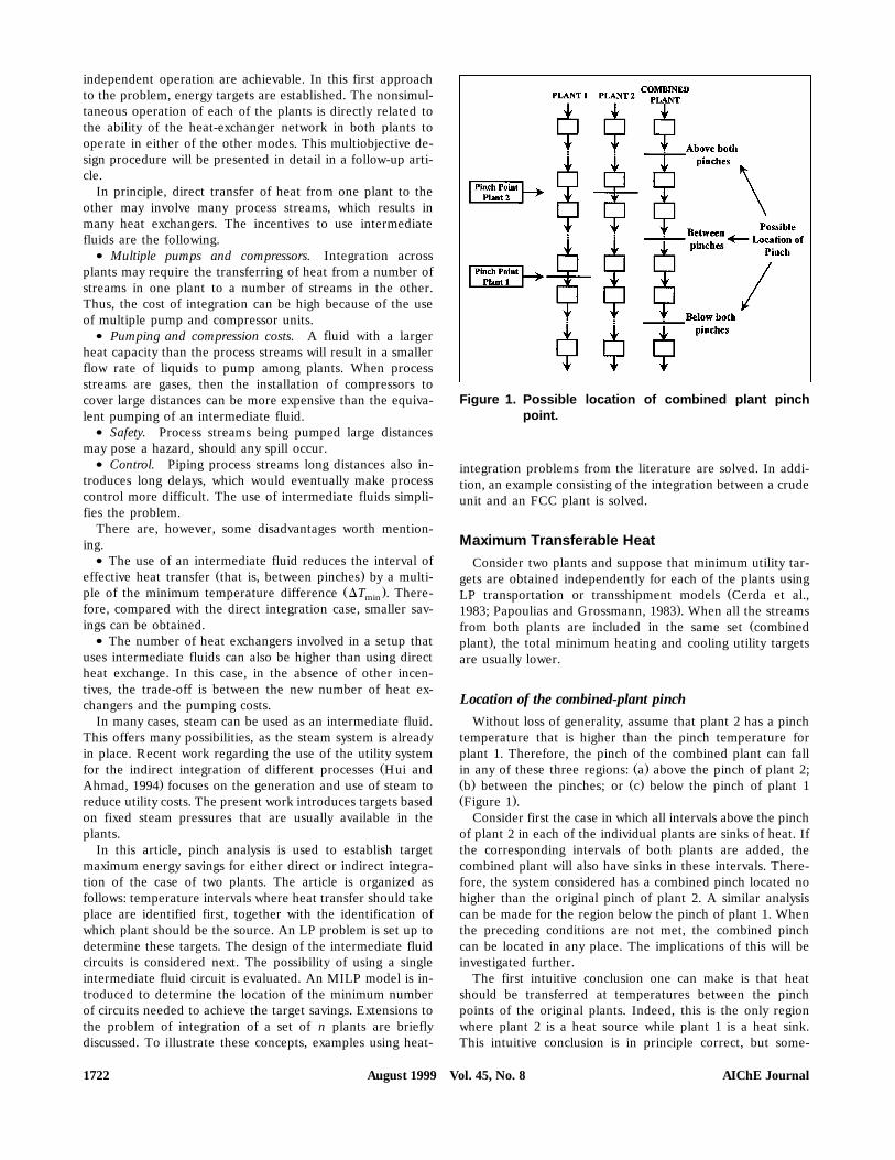
Figure 1. Possible location of combined plant pinchpoint.
integration problems from the literature are solved. In addi-tion, an example consisting of the integration between a crudeunit and an FCC plant is solved.
Maximum Transferable HeatConsider two plants and suppose that minimum utility tar-
gets are obtained independently for each of the plants usingŽLP transportation or transshipment models Cerda et al.,
.1983; Papoulias and Grossmann, 1983 . When all the streamsŽfrom both plants are included in the same set combined
.plant , the total minimum heating and cooling utility targetsare usually lower.
Location of the combined-plant pinchWithout loss of generality, assume that plant 2 has a pinch
temperature that is higher than the pinch temperature forplant 1. Therefore, the pinch of the combined plant can fall
Ž .in any of these three regions: a above the pinch of plant 2;Ž . Ž .b between the pinches; or c below the pinch of plant 1Ž .Figure 1 .
Consider first the case in which all intervals above the pinchof plant 2 in each of the individual plants are sinks of heat. Ifthe corresponding intervals of both plants are added, thecombined plant will also have sinks in these intervals. There-fore, the system considered has a combined pinch located nohigher than the original pinch of plant 2. A similar analysiscan be made for the region below the pinch of plant 1. Whenthe preceding conditions are not met, the combined pinchcan be located in any place. The implications of this will beinvestigated further.
The first intuitive conclusion one can make is that heatshould be transferred at temperatures between the pinchpoints of the original plants. Indeed, this is the only regionwhere plant 2 is a heat source while plant 1 is a heat sink.This intuitive conclusion is in principle correct, but some-
August 1999 Vol. 45, No. 8 AIChE Journal1722

Žtimes heat transfer in the opposite direction from plant 1 to.plant 2 above or below both individual plant pinches is re-
quired to assist the realization of maximum savings.
Transfer of heat outside the region between both pinchpoints
Transferring heat either above the higher pinch or belowthe lower pinch does not decrease the utility usage. Only anequivalent amount of corresponding utility is shifted from oneplant to the other. Figure 2 illustrates the effect of an amountof heat Q transferred from plant 2 to plant 1 in the upperA
Žzone without loss of generality, intervals are lumped to allow.clarity of illustration . An increase of the heating utility in
the plant that releases the heat is followed by a reduction ofthe same utility in the plant that receives the heat. The sameeffect on the cooling needs is observed if a certain amount ofheat Q is transferred from plant 2 to plant 1 in the lowerB
Ž .zone Figure 2 . In addition, as the temperature level at whichthe heat transfer in the upper zone takes place is lowered, amaximum that can be transferred exists. For example, if thetransfer is made in the first interval, the amount that can betransferred is constrained by the original utility usage of plant1, S I . If the heat is transferred in an interval below the firstminone, say interval i, the upper limit will be smaller, as some ofthe utility used by plant 1 is used to satisfy the heat demandof the first iy1 intervals. Therefore, to compute this upperlimit one should subtract all the intervals that are heat sinksŽ . Inegative values above the interval of transfer from S .minSimilar upper limits for the transfer of heat are found if thelower zone is considered.
In conclusion, no savings can be obtained by transferringheat in the regions above the higher pinch or below the lowerpinch. However, transfer from plant 1 to plant 2 in either oneof these regions is needed in some cases to facilitate thetransfer of heat in the region between both pinch tempera-tures. This is explored next.
Transfer of heat between both pinch pointsAs illustrated in Figure 3, a certain amount of heat Q isE
transferred from plant 2 to plant 1 between pinch points. This
Figure 2. Effect of transferring heat outside the regionbetween both pinch temperatures.
Figure 3. Effect of transferring heat in the region be-tween both pinch temperatures.
transfer has the effect of reducing the heating utility in plant1 and cooling utility in plant 2. In addition, transferring heatfrom plant 2 to plant 1 has the effect of reducing the lowestlevel of the heating utility demand on plant 1, which is usu-ally the cheapest. Finally, it has no effect on the heating util-ity of plant 2 or the cooling utility of plant 1.
Assisted and unassisted heat transfer across plantsWe now investigate the upper limits in the amount of heat
that plant 1 can accept and in the amount that plant 2 candeliver in the region between pinches. Consider the case inwhich there are only sink intervals above the pinch point ofplant 2 and only source intervals below the pinch point ofplant 1. The maximum heat that plant 1 can receive is theactual sum of the demands it has in the intervals betweenpinches. Similarly, the maximum amount that plant 2 cantransfer is the resulting available heat it has between pinches.Since any heat that is transferred to plant 1 at any tempera-ture interval can be cascaded down to lower temperatures,the real limitation on how much can be transferred is givenby the ability of plant 2 to fulfill the demand at each interval.Because all the intervals above the pinch point of plant 2 aresinks, the whole demand of the heat in plant 1 is only satis-fied by utility or by plant 2 from the intervals between pinches.Likewise, since all intervals below the pinch point of plant 1are sources of heat, plant 2 does not need to use heat fromthe intervals between pinches to satisfy any demand belowthe pinch point of plant 1. Therefore, the amount of heatthat can be transferred to plant 1 is not limited by such de-mand. This motivates the following definition:
Definition. Unassisted heat transfer across plants takesplace when only heat transfer between pinches is needed toachieve maximum savings.
A special case of unassisted heat transfer across plants iswhen plant 1 has only sink intervals above the pinch point ofplant 2 and only source intervals below the pinch point ofplant 1. Unassisted cases can also take place even thoughsome intervals in plant 1 are sources of heat above the pinchof plant 2 or some intervals in plant 2 are sinks of heat belowthe pinch of plant 1. If a case is unassisted, the combined
August 1999 Vol. 45, No. 8AIChE Journal 1723

Table 1. Example 1
Temp.Plant 1 Plant 2 Combined PlantScale
I I I II II II CP CP CP140 q g S q g S q g Si i min i i min i i min
120 y12 y12 30 y19 y19 20 y31 y31 38
100 y1 y13 y1 y20 y2 y33
80 y15 y28 10 y10 y5 y38I II CPW W Wmin min min60 y2 y30 5 y5 3 y35
40 2 y28 2 1 y4 16 3 y32 6
Max. potential savings between Max. possible savingss12pinches s12
pinch point of both plants lies in between pinches. Indeed,the addition of all intervals and the fact that in general thereis heat transfer across the location of the pinch of plant 2indicates that the pinch does not lie above this temperature.The same can be said for the region below the pinch point ofplant 1.
Assume now that some of the intervals in plant 1 above thelocation of plant 2 pinch are sources of heat. Furthermore,assume such heat sources are enough to produce a surplusthat in the absence of integration across plants is effectivelytransferred in plant 1 through the location of the pinch pointof plant 2. In other words, the surplus of heat above the pinchof plant 2 needs to be used to satisfy the heat demand ofplant 1 between pinches. In turn, this may limit the amountthat can be transferred from plant 2, and therefore limit themaximum savings that can be obtained. To prevent such limi-tation, one can transfer the surplus heat from plant 1 to plant2, reducing the heating utility of plant 2, and allowing maxi-mum heat transfer between pinches. The heat transfer out-side the region between pinches does not realize any savings,only shifts utility load from one plant to the other. In fact, ifthe surplus is larger than the heating utility of plant 2, theamount Q is limited by S II , and the surplus may becomeA minan effective limitation to realize all the potential for savings.
Figure 4. Cascade diagram solution for Example 1.
Similarly, if the heat demand of plant 2 in the correspondingintervals is not sufficiently large, the total surplus that can betransferred is limited. An exact symmetric case happens be-low the pinch of plant 1. Some of the surplus from plant 1below its pinch can eventually be used to satisfy this demand,thus freeing the heat from plant 2 to be completely availableto realize savings through transfer to plant 1 between pinches.
These two cases motivate the following definition.Definition. Assisted heat transfer across plants takes place
when heat transfer between pinches needs to be assisted byheat transfer outside this region to attain maximum savings.
The existence of assisted cases has been overlooked by Ah-Ž .mad and Hui 1991 , who only showed that sometimes more
than one steam level is required for maximum indirect recov-ery between processes. However, they do not explore furtherthe significance of the assisted transfer in order to realize
Ž .maximum savings. Dhole and Linnhoff 1992 construct sitesource and site sink profiles based on the combination ofmodified grand composite curves of the individual processes.In these modified curves process-to-process heat-integrationzones or pockets are eliminated. Consequently, in the pres-ence of an assisted case, opportunities for realizing maximumsavings are lost and only limited savings between pinches canbe pursued.
A model to predict the exact amount of heat that needs tobe transferred in each region is presented later. First, someillustrative examples are shown.
Example of unassisted caseTable 1 shows the interval balances, the heat cascade to
determine the utilities, and the actual value of these utilitiesfor each of the plants as well as for the combined plant. Sinkintervals are located above the pinch and source intervals arelocated below the pinch in either plant 1 or plant 2. There-fore, this is an unassisted case, and only transfer betweenpinches is needed in order to obtain maximum savings. Thesesavings are obtained by subtracting from the sum of the indi-vidual utilities the combined utility. Pinch locations are shownwith filled lines. As expected, the combined pinch is in be-tween the original plant pinches. Figure 4 shows the cascadediagram solution after the integration is conducted.
In order to compare the results obtained using the cascadediagram with methods that make use of grand composite
Figure 5. Countercurrent composite curve profiles forExample 1.
August 1999 Vol. 45, No. 8 AIChE Journal1724
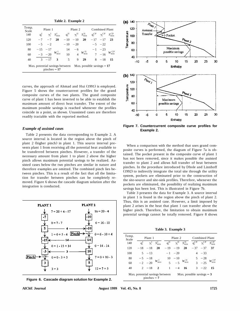
Table 2. Example 2
Temp.Plant 1 Plant 2 Combined PlantScale
I I I II II II CP CP CP140 q g S q g S q g Si i min i i min i i min
120 y7 y7 20 y10 y10 20 y17 y17 23
100 y5 y2 y10 y20 y5 y22
80 y15 y17 14 y6 y1 y23I II CPW W Wmin min min60 y3 y20 10 4 7 y16
40 3 y17 3 5 9 29 8 y18 15
Max. potential savings between Max. possible savingss17pinches s17
Ž .curves, the approach of Ahmad and Hui 1991 is employed.Figure 5 shows the countercurrent profiles for the grandcomposite curves of the two plants. The grand compositecurve of plant 1 has been inverted to be able to establish themaximum amount of direct heat transfer. The extent of themaximum possible savings is reached whenever the profilescoincide in a point, as shown. Unassisted cases are thereforereadily tractable with the reported method.
Example of assisted casesTable 2 presents the data corresponding to Example 2. A
source interval is located in the region above the pinch ofŽ .plant 2 higher pinch in plant 1. This source interval pre-
vents plant 1 from receiving all the potential heat available tobe transferred between pinches. However, a transfer of thenecessary amount from plant 1 to plant 2 above the higherpinch allows maximum potential savings to be realized. As-sisted cases below the two pinches are similar in nature andtherefore examples are omitted. The combined pinch lies be-tween pinches. This is a result of the fact that all the limita-tion for transfer between pinches can be completely re-moved. Figure 6 shows the cascade diagram solution after theintegration is conducted.
Figure 6. Cascade diagram solution for Example 2.
Figure 7. Countercurrent composite curve profiles forExample 2.
When a comparison with the method that uses grand com-posite curves is performed, the diagram of Figure 7a is ob-tained. The pocket present in the composite curve of plant 1has not been removed, since it makes possible the assistedtransfer to plant 2 and allows full transfer of heat betweenpinches. In the procedure introduced by Dhole and LinnhoffŽ .1992 to indirectly integrate the total site through the utilitysystem, pockets are eliminated prior to the construction ofthe site-source and site-sink profiles. Therefore, whenever thepockets are eliminated, the possibility of realizing maximumsavings has been lost. This is illustrated in Figure 7b.
Table 3 presents the data for Example 3. A source intervalin plant 1 is found in the region above the pinch of plant 2.Thus, this is an assisted case. However, a limit imposed byplant 2 arises in the heat that plant 1 can transfer above thehigher pinch. Therefore, the limitation to obtain maximumpotential savings cannot be totally removed. Figure 8 shows
Table 3. Example 3
Temp.Plant 1 Plant 2 Combined PlantScale
I I I II II II CP CP CP140 q g S q g S q g Si i min i i min i i min
120 y18 y18 20 y19 y19 20 y37 y37 37
100 5 y13 y1 y20 4 y33
80 y5 y18 10 y10 5 y28I II CPW W Wmin min min60 y2 y20 5 y5 3 y25
40 2 y18 2 1 y4 16 3 y22 15
Max. potential savings between Max. possible savingss3pinches s7
August 1999 Vol. 45, No. 8AIChE Journal 1725
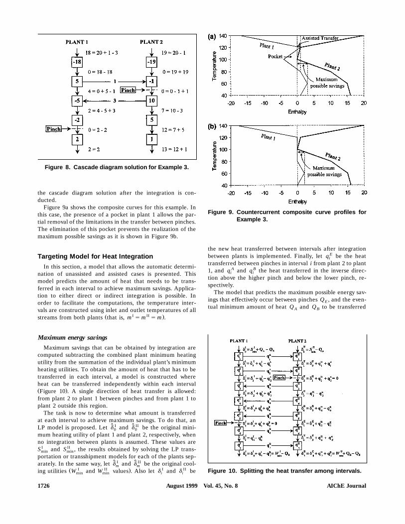
Figure 8. Cascade diagram solution for Example 3.
the cascade diagram solution after the integration is con-ducted.
Figure 9a shows the composite curves for this example. Inthis case, the presence of a pocket in plant 1 allows the par-tial removal of the limitations in the transfer between pinches.The elimination of this pocket prevents the realization of themaximum possible savings as it is shown in Figure 9b.
Targeting Model for Heat IntegrationIn this section, a model that allows the automatic determi-
nation of unassisted and assisted cases is presented. Thismodel predicts the amount of heat that needs to be trans-ferred in each interval to achieve maximum savings. Applica-tion to either direct or indirect integration is possible. Inorder to facilitate the computations, the temperature inter-vals are constructed using inlet and outlet temperatures of all
Ž I II .streams from both plants that is, m s m s m .
Maximum energy sa©ingsMaximum savings that can be obtained by integration are
computed subtracting the combined plant minimum heatingutility from the summation of the individual plant’s minimumheating utilities. To obtain the amount of heat that has to betransferred in each interval, a model is constructed whereheat can be transferred independently within each intervalŽ .Figure 10 . A single direction of heat transfer is allowed:from plant 2 to plant 1 between pinches and from plant 1 toplant 2 outside this region.
The task is now to determine what amount is transferredat each interval to achieve maximum savings. To do that, an
ˆI ˆIILP model is proposed. Let d and d be the original mini-0 0mum heating utility of plant 1 and plant 2, respectively, whenno integration between plants is assumed. These values areS I and S II , the results obtained by solving the LP trans-min minportation or transshipment models for each of the plants sep-
ˆI ˆIIarately. In the same way, let d and d be the original cool-m mŽ I II . I IIing utilities W and W values . Also let d and d bemin min i i
Figure 9. Countercurrent composite curve profiles forExample 3.
the new heat transferred between intervals after integrationbetween plants is implemented. Finally, let q E be the heatitransferred between pinches in interval i from plant 2 to plant1, and q A and q B the heat transferred in the inverse direc-i ition above the higher pinch and below the lower pinch, re-spectively.
The model that predicts the maximum possible energy sav-ings that effectively occur between pinches Q , and the even-Etual minimum amount of heat Q and Q to be transferredA B
Figure 10. Splitting the heat transfer among intervals.
August 1999 Vol. 45, No. 8 AIChE Journal1726

in the regions outside the one between pinches is
Min d Iqd IIŽ .0 m
s.t.
I ˆId sd qQ yQ0 0 A E
II ˆIId sd yQ0 0 A
d I sd I q q I y q Ai iy1 i i II; is1, . . . , pII II II A 5d sd q q q qi iy1 i i
d I sd I q q I q q Ei iy1 i i II I; is p q1 , . . . , p 1Ž .Ž .II II II E 5d sd q q y qi iy1 i i
d I sd I q q I y q Bi iy1 i i I; is p q1 , . . . , mŽ .II II II B 5d sd q q q qi iy1 i i
I ˆId sd yQm m B
II ˆIId sd qQ yQm m B E
d II s0, d II
II s0p p
d I , d II , q A, q E, q BG0.i i i i i
In this formulation pI and pII are the respective pinchpoint levels, and it is assumed pI - pII. The problem consid-ers the conditions of minimum utility usage for both plants asthe starting point. The objective function used needs someexplanation. Minimizing the utility needed in plant 1 servestwo purposes:
1. To reduce the utility in the amount transferred fromplant 2 between pinches.
2. To make sure that the amount of heat transferred fromplant 1 to plant 2 is strictly the minimum needed.
When a higher amount of heat than the minimum neededis transferred above pinches in the assisted case, the excessconsists of a simple shift of utility from plant 2 to plant 1.Such shifting requires equipment and therefore representsadditional investment without a benefit and should beavoided. The same result is obtained if one solves the prob-lem minimizing the amount of cooling utility of plant 2. Inthis case, the transfer to plant 1 is maximized, while thetransfer from plant 1 to plant 2 below both pinches is kept atits minimum necessary to assist in the savings. Finally, foreach unit of heat transferred between plants, both values arereduced by the same amount simultaneously. This implies thatindependent reductions of these utilities are not possible.Hence, adding them to form the objective function of prob-lem 1 is possible. A simple balance around plant 1 proves
Žthat the summation of the solutions heat transferred amountsE.q will represent the total possible amount of heat to bei
transferred between pinches Q .ERemark. The LP problem presented has degenerate solu-
tions. Indeed, to transfer heat surplus from an interval in plant2 to any interval in plant 1 between pinches, the heat can betransferred from plant 2 to plant 1 first and then transferreddown, or transferred down in plant 2 first, and then trans-
ferred to plant 1 at a lower interval. The same situations oc-cur in an inverse manner when the transfer takes place in anyof the regions outside the region between pinches. There-fore, many different paths are available. This degeneracy isactually a flexibility that can be exploited later when a designis attempted.
The results from the preceding models can now be usedas target values for models that will determine the heat-exchanger network needed to accomplish such savings. Inparticular, the knowledge of what are the intervals at whichheat transfer from one plant to the other should take placeŽ .in addition to the direction of such transfer is a useful inputfor these models. These models, which will be presented in afollow-up article will address the design of systems featuringthe minimum number of exchanger units to accomplish a dual
Ž .operation with and without integration .
Indirect Heat IntegrationThe focus is now on the case of indirect heat integration by
the use of intermediate fluid circuits. The design parametersfor these circuits, namely flow rate and inlet and outlet tem-peratures, have to be calculated.
Shift of scalesWhen an intermediate fluid is used, new streams appear in
each plant. Consider the region between pinches first. In plant1, the intermediate fluid acts as a hot stream, whereas inplant 2, it acts as a cold stream. The temperature of the in-
Ž .termediate fluid leaving plant 1 registered in its hot scaleshould be equal to the starting temperature of the same fluidin plant 2, requiring the coincidence between the respectivehot and cold scales. Thus, a shift consisting of moving the hot
Ž .scale of plant 2 and with it, the cold scale too downwardDT degrees in the region below its pinch is performed.minNow consider the possibility of assisted cases. In the regionabove the higher pinch and below the lower pinch, the fluidcirculates in the inverse direction than between pinches.Therefore, a match between the cold scale of plant 1 and thehot scale of plant 2 is required in these two regions. To ac-
Žcomplish this, the hot scale of plant 2 and with it, the cold.scale is shifted upward DT degrees in the zone above itsmin
pinch. Similarly, in the region below the lower pinch, a shiftŽ .of the hot scale of plant 1 and with it, the cold scale down-
ward is needed. However, the hot scale of plant 2 was al-ready shifted by DT . Therefore, a shift of 2DT degreesmin min
Ždownward of the hot scale of plant 1 and, with it, its cold.scale has to be performed. Finally, as in the direct integra-
tion case, the temperature intervals are constructed using in-let and outlet temperatures of all streams of both plants.
As a result of these temperature shifts, smaller savings thanin the direct integration case may be achieved. If the use of
Žintermediate fluids is not mandatory due to safety or other.considerations , then this reduction in savings potential may
or may not be compensated by the reduction in piping,pumping, andror compression costs.
Summarizing, the scale shifts required are:1. A shift of both hot and cold scales downward by DTmin
degrees in plant 2 below its pinch.
August 1999 Vol. 45, No. 8AIChE Journal 1727
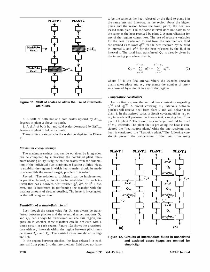
Figure 11. Shift of scales to allow the use of intermedi-ate fluids.
2. A shift of both hot and cold scales upward by DTmindegrees in plant 2 above its pinch.
3. A shift of both hot and cold scales downward by 2DTmindegrees in plant 1 below its pinch.
These shifts create gaps in the scales, as depicted in Figure11.
Maximum energy sa©ingsThe maximum savings that can be obtained by integration
can be computed by subtracting the combined plant mini-mum heating utility using the shifted scales from the summa-tion of the individual plant’s minimum heating utilities. Next,to establish the regions in which heat transfer should be madeto accomplish the overall target, problem 1 is solved.
Remark. The solution to problem 1 can be implementedin practice. Indeed, a circuit can be established for each in-terval that has a nonzero heat transfer q E, q A, or q B. How-i i iever, one is interested in performing the transfer with thesmallest amount of circuits possible. The issue is investigatedin the following sections.
Feasibility of a single-fluid circuitEven though the target value for Q can always be trans-E
ferred between pinches and the eventual target amounts QAand Q can always be transferred outside this region, theBquestion is whether these transfers can be achieved with asingle circuit in each region. Figure 12a shows the unassistedcase with m intervals within the region between pinch tem-Eperatures T II and T I . The assisted cases are shown in Fig-p pure 12b.
In the region between pinches, the heat released in eachinterval from plant 2 to the intermediate fluid does not have
to be the same as the heat released by the fluid to plant 1 inthe same interval. Likewise, in the region above the higherpinch and the region below the lower pinch, the heat re-leased from plant 1 in the same interval does not have to bethe same as the heat received by plant 2. A generalization forany of the regions comes next. The use of separate variablesfor the heat transferred to and from the intermediate fluidare defined as follows: q FC for the heat received by the fluidiin interval i, and q FH for the heat released by the fluid iniinterval i. The total heat transferred Q is already given byFthe targeting procedure, that is,
k Fq m k Fq mK KFC FHQ s q s q , 2Ž .Ý ÝF i i
F Fis k is k
where k F is the first interval where the transfer betweenplants takes place and m represents the number of inter-Kvals covered by a circuit in any of the regions.
Temperature constraintsLet us first explore the second law constraints regarding
q FC and q FH. A circuit covering m intervals betweeni i Epinches will receive heat from plant 2 and will deliver it toplant 1. In the assisted cases, a circuit covering either m orAm intervals will perform the inverse task, carrying heat fromBplant 1 to plant 2. Therefore, this can be generalized for a setof m intervals. The plant that is providing the heat is con-Ksidered the ‘‘heat-source plant,’’ while the one receiving thatheat is considered the ‘‘heat-sink plant.’’ The following con-straints prevent the temperature of the fluid from going
Figure 12. Circuits of intermediate fluids in unassisted(and assisted cases gaps are omitted for
)simplicity .
August 1999 Vol. 45, No. 8 AIChE Journal1728

higher than the interval temperature T in the heat-sourceky1plant:
k Fq m KFC FC F FF T yT G q ;ks k qm , . . . , k q1Ž .Ž . Ž .Ýky1 0 i K
is k
3Ž .
F T FCF yT FC sQ . 4Ž .Ž .k y1 0 F
In the heat-sink plant, similar constraints are introduced toprevent the temperature of the fluid going lower than theinterval temperature T :k
kFH FH F FF T yT G q ;ks k , . . . , k q m y1Ž . Ž .Ý0 k i K
Fis k
5Ž .
F T FHyT FHF sQ . 6Ž .Ž .0 k qm FK
In order to assure a closed circuit, it should be noticed thatthe following has to be verified:
T FCsT FHF 7Ž .0 k qm K
T FHsT FCF . 8Ž .0 k y1
Let us now examine what values the initial temperatures ofthe intermediate fluid can take. First, note that to guaranteefeasibility of heat transfer, T FC and T FH are equal to T0 0 ky1
Žand T , respectively, for some k that is, they are confined tok.be end-interval temperatures . Now consider the case where
the heat-source plant does not have any heat demand in theŽ q F . FH Ffirst set of k y k q1 intervals, that is, q s0, ; is k ,i
. . . , kq. Then by increasing the flow rate of the intermediatefluid and without limitations in the transfer of heat from theheat-source plant, a new solution with an upper temperaturesmaller than the one considered initially is possible. If this isthe case, the heat-source plant will only be transferring heatto the intermediate fluid at temperatures lower than T q. Tokfind such a solution, heat can be cascaded down from the
Ž q F .first k y k q1 intervals in the heat-source plant. The val-ues of q FC can be transformed to a new set q FC as follows:ˆi i
q FCs0 ; is k F, . . . , kq 9Ž .i
kq
FC FC FCq qq s q q q 10Ž .ˆ Ýk q1 k q1 i
Fis k
q FCs q FC ; is kqq2, . . . , k Fq m , 11Ž .ˆ Ž .i i K
where q FC is another degenerate solution. This solution al-ilows the circuit to be established between the intervals kqq1
Ž F .and k q m . A similar argument can be made for the caseKwhere the last intervals in plant 2 do not transfer heat to theintermediate fluid.
Thus, one can assume without loss of generality that theinitial temperatures of the intermediate fluid in the heat-
source and sink plants are
T FCsT FHF sT F 12Ž .0 k qm k qmK K
T FHsT FCF sT F . 13Ž .0 k y1 k y1
With these equalities, the set of Eqs. 3]6 become
kFH F F
FF T yT G q ;ks k , . . . , k q m y1Ž . Ž .Ýk y1 k i KFis k
14Ž .
k Fq m KFC F
FF T yT G q ;ks k q1, . . . , mŽ . Ž .Ýk k qm i KKis k
15Ž .
F T F yT F sQ 16Ž .Ž .k y1 k qm FK
Equations 14]16 constitute a feasibility test for a singlecircuit transferring the heat Q between plants. The flow rateFF can be calculated using Eq. 16. This value then can bereplaced in Eqs. 14 and 15. If any of these equations are notsatisfied, then a circuit between T F and T F cannotk y1 k qm K
transfer the maximum amount, but perhaps some smallervalue.
Candidate heat-transfer setsThe flexibility at hand for defining the general variables
q FH and q FC is explored by an adjusted heat-cascaded dia-i iŽ .gram Figure 13 . The target values Q , Q , and Q areE A B
added and subtracted in the three defined zones of the cas-cade. This accounts for the supplies or demand each of the
(Figure 13. Adjusted heat-cascaded diagram gaps are)omitted for simplicity .
August 1999 Vol. 45, No. 8AIChE Journal 1729

zones will experience when the respective single-circuit can-didates are considered. The values obtained for the differentintervals are not realistic heat-transfer amounts since someof them are negative, but rather a calculation aid. Moreover,because of these operations the adjusted heat-cascaded dia-gram of the heat-source plant may exhibit an induced pinchat each region where a circuit can be installed. In this in-stance, the transfer will only occur in the subzone delimitedby the real and induced pinches.
In the unassisted case, the solutions of Eq. 1 satisfy thefollowing relations:
kI I I Eˆ IId sd yQ q q q q G0Ž .Ýk p E i i
IIis p q1
;ks pII q1 , . . . , pI 17Ž .Ž .k
II II Ed s q y q G0Ž .Ýk i iIIis p q1
;ks pII q1 , . . . , pI . 18Ž .Ž .
The same set of equations can be written in terms of q EHi
and q EC:i
kI I I E Hˆ IId sd yQ q q q q G0Ž .Ýk p E i i
IIis p q1
;ks pII q1 , . . . , pI 19Ž .Ž .k
II II ECd s q y q G0Ž .Ýk i iIIis p q1
;ks pII q1 , . . . , pI . 20Ž .Ž .
Similarly, for the assisted cases the relations for the upperand lower zones are:
kI I I ACˆd sd qQ yQ q q y q G0Ž .Ýk 0 A E i i
is1
;ks1, . . . , pII 21Ž .k
II II II A Hˆd sd yQ q q q q G0Ž .Ýk 0 A i iis1
;ks1, . . . , pII 22Ž .k
I I BCd s q y q G0Ž .Ýk i iIis p q1
;ks pI q1 , . . . , m 23Ž .Ž .k
II I II BHˆ Id sd yQ q q q q G0Ž .Ýk p E i iIIis p q1
;ks pI q1 , . . . , m. 24Ž .Ž .
Thus, any nonnegative set of generalized values q FH andiq FC that satisfies Eqs. 19]20, 21]22, or 23]24, and also thei
Ž .balance equation Eq. 2 is an acceptable candidate for a sin-gle circuit. If in addition, Eqs. 14]16 are satisfied, the candi-date set will be a feasible single-circuit solution in any of thezones. A few generalized candidate sets are presented next.
One candidate set is given by the solution of problem 1,that is,
q FHs q FCs q F. 25Ž .i i i
Other sets can be found by making use of degeneracy. Inparticular, one can choose a set that prioritizes the heattransfer to the intermediate fluid over the heat transfer tothe interval below in the source plant. This solution is calledthe higher-circuit solution, because the circuit starts and endsat the higher possible intervals. A lower circuit solution ispresented later. The maximization of the heat delivered tothe intermediate fluid is the purpose of constructing a highercircuit solution.
Therefore, to establish the maximum amount of heat thateach interval can provide to the intermediate fluid, the deficitof heat in the intervals below it need to be taken into ac-count. The heat availability v H at each interval is then de-k
H � H 4 H � H 4fined as follows: Let l sMin q , 0 and s sMax q , 0k k k k;ks k Fq1, . . . , k Fq m . In addition, let lH
F s0, s HF s q H
Fk k k kˆH H
Fqd . Thus, the availability v is given byk y1 k
lHF qs H
F q HF q lH
F -0k qm k qm k qm k qmK K K KHFz s 26Ž .k qm K H H½ F F0 q q l G0k qm k qmK K
z H q lHqs H q Hq z H q lH-0kq1 k k k kq1 kHz sk H H H½ 0 q q z q l G0k kq1 k
;ks k Fq1, . . . , k Fq m y1. 27Ž .K
z HF q lH
F qs HF q H
F q z HF q lH
F -0k q1 k k k k q1 kHFz s 28Ž .k H H H½ F F F0 q q z q l G0k k q1 k
v HsMax q Hq z H q lH, 0 ;ks k F, . . . , k Fq m .� 4k k kq1 k K
29Ž .
In these equations, z H is an auxiliary variable that helpskŽdetermine the amount of cumulative demand from the bot-
.tom at every interval. To illustrate this, consider first theˆH
Fsituation depicted in Table 4 for which d s0, that is,k y1
Table 4. Determination of Heat Availability
H H H H H H H HInterval q l s q q z q l z vi k k k kq1 k k kFk 12 0 12 8 0 8
Fk q1 y1 y1 0 y5 y4 0Fk q2 y1 y1 0 y4 y3 0Fk q3 15 0 15 y2 y2 0Fk q4 y15 y15 0 y32 y17 0Fk q5 y2 y2 0 y4 y2 0Fk q6 20 0 20 20 0 20
August 1999 Vol. 45, No. 8 AIChE Journal1730
either a higher circuit between pinches or a circuit above allpinches with an induced pinch.
Under such conditions, all resulting heat flows cascadeddown are positive. On the source side, the higher-circuit solu-tion is given by
q FCF sMin v H
F , Q 30Ž .� 4k k F
k y1FC H FC F Fq sMin v , Q y q ;ks k q1, . . . , k q m .Ýk k F i K½ 5
Fis k
31Ž .
Equation 30 states that at the first interval, all the heatavailable will be used provided it is lower than the overallmaximum. Equation 31 states that at every interval, the maxi-mum that can be transferred is the surplus. In turn, for thesink plant, the higher solution is
q FHF sQ 32Ž .k F
q FHs0 ;ks k Fq1, . . . , k Fq m . 33Ž .k K
This means that if the sink plant can transfer all the maxi-mum possible heat Q in the first interval of transfer k F,Fthen the higher-circuit solution will consist of this intervalonly.
At the other extreme, we have a solution that maximizesthe transfer of heat to the interval below in the heat-sourceplant, minimizing the transfer to the intermediate fluid. Thissolution is called the lower-circuit solution because it startsand ends at the lowest intervals possible. In such case, thesolutions for the sink and the source plants are somewhatrelated. Indeed, by transferring heat to lower intervals in thesource plant, one must make sure that the plant does notneed the heat at the same interval. The adjusted cascadedheat values already account for this. Then, the lower-circuitsolution for the sink plant is given by
q FHF sMax yu C
F , 0 34Ž .� 4k k
k y1FH C FH F Fq sMax yu y q , 0 , ;ks k q1, . . . , k q m .Ýk k i K½ 5
Fis k
35Ž .
Now let kq be the first interval with nonzero heat trans-ferred from the intermediate fluid to the sink plant, that is,
q FH F Ž q . FHqk is such that q s0, ;ks k , . . . , k y1 ; q /0. Next,k k
all the surplus heat in the source plant can be transferreddown until interval kq is reached. From then on, only theminimum amount of heat should be transferred to the inter-mediate fluid. This minimum should be at least equal to q FH
ito guarantee that temperature constraints have a chance ofbeing satisfied. Thus, the lower-circuit solution for the sourceplant is
q FCs0 ;ks k F, . . . , kqy1 36Ž . Ž .k
q FCs q FH ;ks kq, . . . , k Fq m . 37Ž .k k K
By construction, no one-circuit solution can:1. Start at a lower interval;2. Transfer less heat from the intermediate fluid to the sink
plant at any interval defined by the lower solution.As a result of the calculation of the cumulative heat de-
mands, a limit for the starting point of the unique circuit isestablished. In view of the preceding, a second test for thefeasibility of a single circuit transferring the maximum sav-ings Q in any of the regions consists of constructing theFhigher or lower solution and checking if the following equa-tions are satisfied:
kFT yTŽ .k y1 k FHQ G qÝF iF FT yTŽ . Fk y1 k qm K is k
;ks k F, . . . , k Fq m y1 38Ž .Ž .K
k Fq m KFT yTŽ .k k qm K ECQ G qÝF iF FT yTŽ .k y1 k qm is kK
;ks k Fq m , . . . , k Fq1 . 39Ž . Ž .Ž .K
These equations have been obtained by substituting Eq. 16 inEqs. 14 and 15.
It should be noted that the lower solution obtained by thepreceding procedure is not always feasible. Some other lowersolutions might exist, not necessarily covering the last inter-vals of the region between pinches, but covering a region thatends somewhere above it.
Example 4In this example, Test Case a2 from Linnhoff and Hind-
Ž .marsh 1983 is plant 1 and problem 4sp1 is plant 2. The datafor the separate plants are shown in Table 5. Note that DTminfor plant 1 is 208C, while DT for plant 2 is 108C. Pinchmintemperatures and minimum utility consumption for each ofthe plants are shown in Table 6.
Direct Integration Solution. Table 7 shows the results ofthe pinch analysis. The interval between pinches goes from
Table 5. Data for Example 4
F T T Qs tŽ . Ž . Ž . Ž .Streams kWr8C 8C 8C kW
Test Case a2Ž .H1 Hot 2.0 150 60 180.0Ž .C2 Cold 2.5 20 125 262.5Ž .H3 Hot 8.0 90 60 240.0Ž .C4 Cold 3.0 25 100 225.0
Ž .S Stream } 270 270 107.5Ž .CW Water 0.9 38 82 40.0
DT s208Cmin
Problem 4sp1Ž .C1 Cold 7.62 60 160 762Ž .H2 Hot 8.79 160 93 589Ž .C3 Cold 6.08 116 260 876Ž .H4 Hot 10.55 249 138 1171
Ž .S Steam } 270 270 128Ž .CW Water 5.68 38 82 250
DT s108Cmin
August 1999 Vol. 45, No. 8AIChE Journal 1731

Table 6. Individual Plant Pinch Analysis for Example 4
Pinch Heating Utility Cooling UtilityŽ . Ž . Ž .Problem Temp. 8C kW kW
Test case a2 90 107.5 40.04sp1 249 128.0 250.0
908C to 2498C. After considering all streams in a single set,Žthe resulting combined pinch is located at 2498C upper limit
.of the interval between pinches . This is the consequence ofthe large availability of heat to transfer that plant 2 has in allthe intervals between pinches. This amount of heat is suffi-cient to supply the entire demand of plant 1. Therefore, themaximum possible heat savings for the direct integration arethe original minimum utility of plant 1, that is 107.5 kW. Thisis also the result obtained by solving problem 1.
Indirect Integration Solutions. After the hot temperaturescale in plant 2 is shifted down 108C, the interval betweenpinches is from 2398C to 908C. Table 8 shows the pinch anal-ysis for the indirect integration. The combined pinch then
Ž .results at the upper bound 2398C . Fewer intervals than inthe case of direct integration are found, since some of theextreme temperatures now coincide due to the shift. The so-lution of problem 1 is Q s107.5 kW, which is equal to theFmaximum possible savings that can be obtained either withdirect or indirect integration. Therefore, in this case the shiftdoes not have any effect in reducing the amount that can betransferred between pinches. Table 8 shows that there is nodemand in the upper intervals of plant 1, and the shift doesnot appreciably decrease the large availability of heat in plant2 in the region between pinches.
An implementation of this indirect integration follows. Thetest of feasibility for a single circuit is applied first to a circuitcovering all the intervals between pinches. This solution isfeasible, and Table 9 shows the values obtained for the pa-
Table 7. Pinch Analysis for Direct Integration inExample 4
Test Case a2 4sp1 Combined PlantI I I II II II C C C PT q g S q g S q g Si i min i i min i i min
Ž . Ž . Ž . Ž . Ž . Ž . Ž . Ž . Ž . Ž .8C kW kW kW kW kW kW kW kW kW
270 0 0 107.5 y127.8 y127.8 127.8 y127.8 y127.8 127.8
249 0 0 353.1 225.3 353.1 225.3170 0 0 y31.5 193.8 y31.5 193.8160 0 0 56.4 250.2 56.4 250.2150 10.0 10.0 28.2 278.4 38.2 288.4145 y3.5 6.5 39.5 317.9 36.0 324.4138 y6.0 0.5 y58.9 259.0 y64.9 259.5126 y3.0 y2.5 7.0 266.0 4.0 263.5120 y94.5 y97.0 31.6 297.6 y62.9 200.693 y10.5 y107.5 y22.9 274.7 y33.4 167.2
90 90.0 y17.5 y152.4 122.3 y62.4 104.8I II C PW W Wmin min min70 45.0 27.5 0 122.3 45.0 149.8Ž . Ž . Ž .kW kW kW60 y82.5 y55.0 0 122.3 y82.5 67.345 y12.5 y67.5 40.0 0 122.3 250.0 y12.5 54.8 182.5
Table 8. Pinch Analysis for Indirect Integration inExample 4
Test Case a2 4sp1 Combined PlantI I I II II II C C C PT q g S q g S q g Si i min i i min i i min
Ž . Ž . Ž . Ž . Ž . Ž . Ž . Ž . Ž . Ž .8C kW kW kW kW kW kW kW kW kW
260 0 0 107.5 y127.8 y127.8 127.8 y127.8 y127.8 127.8
239 0 0 353.1 225.3 353.1 225.3160 0 0 y31.5 193.8 y31.5 193.8150 10.0 10.0 28.2 222.0 38.2 232.0145 y8.5 1.5 95.8 317.8 87.3 319.3128 y4.0 y2.5 y39.3 278.5 y43.3 276.0120 y14.0 y16.5 y19.6 258.9 y33.6 242.4116 y91.0 y107.5 30.4 289.3 y60.6 181.8
90 31.5 y76.0 8.2 297.5 39.7 221.5I II C PW W Wmin min min83 103.5 27.5 y175.3 122.2 y71.8 149.7Ž . Ž . Ž .kW kW kW60 y82.5 y55.0 0 122.2 y82.5 67.245 y12.5 y67.5 40.0 0 122.2 250.0 y12.5 54.7 182.5
Table 9. Some of the Indirect Solutions to Example 4
No. of T T Fup downŽ . Ž . Ž .Solution Intervals 8C 8C kWr8C
All intervals 7 239 90 0.721Lower circuit 5 150 90 1.792Higher circuit 2 239 150 1.208
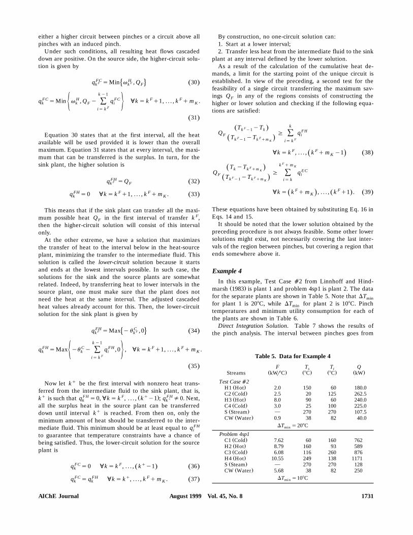
Žrameters ending temperatures and rate]heat-capacity prod-.uct . The higher-circuit solution is shown in Table 10. The
position of the resulting circuit is shown in Figure 14. Notethat Eqs. 38 and 39 are satisfied. Moreover, the intermediatesolutions between the circuit spanning all intervals and thehighest possible circuit are feasible.
Finally, the lower-circuit solution is presented in Table 11,and its position is shown in Figure 15. The intermediate cir-cuits between the circuit spanning all intervals and the lowestpossible circuit are proven feasible. Other solutions can befound each time that a certain amount of heat could be cas-caded and the one-circuit solutions that result are feasible.However, no solution will be able to start below the limitestablished by the lower solution. In this sense, the problemhas a large finite number of possible solutions that requirefurther analysis, taking into account the resulting heat-ex-changer network and the economic aspects.
Table 10. ‘‘Higher Circuit’’ Solution to Example 4
Test Case a2 4sp1Q s107.5 kWEI E H II II ECŽ . Ž . Ž . Ž . Ž .Interval q kW q kW q kW v kW q kWk k k k k
IIp q1s2 0 107.5 353.1 321.6 107.5IIp q2s3 0 0 y31.5 0 0IIp q3s4 10 0 28.2 28.2 0IIp q4s5 y8.5 0 95.8 36.9 0IIp q5s6 y4.0 0 y39.3 0 0IIp q6s7 y14.0 0 y19.6 0 0IIp q7s8 y91.0 0 30.4 30.4 0
August 1999 Vol. 45, No. 8 AIChE Journal1732
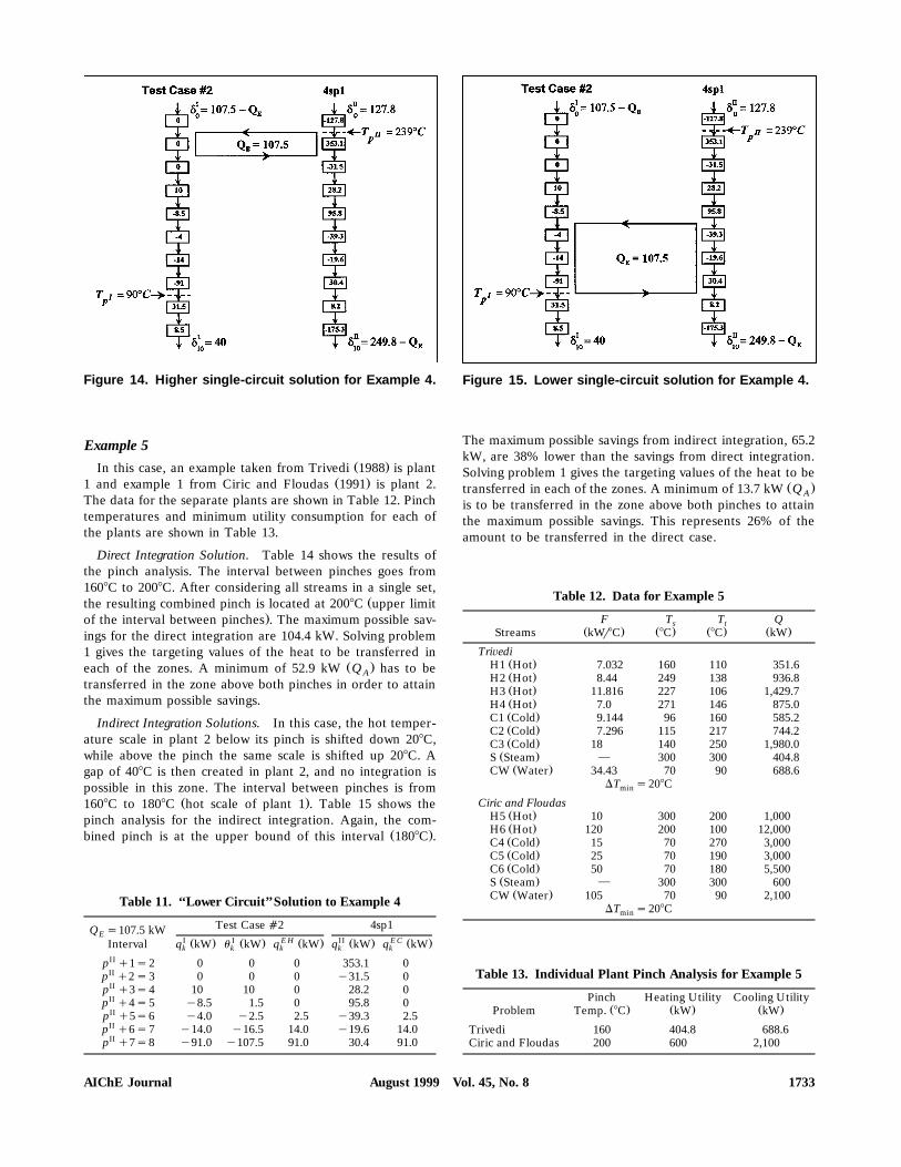
Figure 14. Higher single-circuit solution for Example 4.
Example 5Ž .In this case, an example taken from Trivedi 1988 is plant
Ž .1 and example 1 from Ciric and Floudas 1991 is plant 2.The data for the separate plants are shown in Table 12. Pinchtemperatures and minimum utility consumption for each ofthe plants are shown in Table 13.
Direct Integration Solution. Table 14 shows the results ofthe pinch analysis. The interval between pinches goes from1608C to 2008C. After considering all streams in a single set,
Žthe resulting combined pinch is located at 2008C upper limit.of the interval between pinches . The maximum possible sav-
ings for the direct integration are 104.4 kW. Solving problem1 gives the targeting values of the heat to be transferred in
Ž .each of the zones. A minimum of 52.9 kW Q has to beAtransferred in the zone above both pinches in order to attainthe maximum possible savings.
Indirect Integration Solutions. In this case, the hot temper-ature scale in plant 2 below its pinch is shifted down 208C,while above the pinch the same scale is shifted up 208C. Agap of 408C is then created in plant 2, and no integration ispossible in this zone. The interval between pinches is from
Ž .1608C to 1808C hot scale of plant 1 . Table 15 shows thepinch analysis for the indirect integration. Again, the com-
Ž .bined pinch is at the upper bound of this interval 1808C .
Table 11. ‘‘Lower Circuit’’ Solution to Example 4
Test Case a2 4sp1Q s107.5 kWEI I E H II ECŽ . Ž . Ž . Ž . Ž .Interval q kW u kW q kW q kW q kWk k k k k
IIp q1s2 0 0 0 353.1 0IIp q2s3 0 0 0 y31.5 0IIp q3s4 10 10 0 28.2 0IIp q4s5 y8.5 1.5 0 95.8 0IIp q5s6 y4.0 y2.5 2.5 y39.3 2.5IIp q6s7 y14.0 y16.5 14.0 y19.6 14.0IIp q7s8 y91.0 y107.5 91.0 30.4 91.0
Figure 15. Lower single-circuit solution for Example 4.
The maximum possible savings from indirect integration, 65.2kW, are 38% lower than the savings from direct integration.Solving problem 1 gives the targeting values of the heat to be
Ž .transferred in each of the zones. A minimum of 13.7 kW QAis to be transferred in the zone above both pinches to attainthe maximum possible savings. This represents 26% of theamount to be transferred in the direct case.
Table 12. Data for Example 5
F T T Qs tŽ . Ž . Ž . Ž .Streams kWr8C 8C 8C kW
Tri®ediŽ .H1 Hot 7.032 160 110 351.6Ž .H2 Hot 8.44 249 138 936.8Ž .H3 Hot 11.816 227 106 1,429.7Ž .H4 Hot 7.0 271 146 875.0Ž .C1 Cold 9.144 96 160 585.2Ž .C2 Cold 7.296 115 217 744.2Ž .C3 Cold 18 140 250 1,980.0
Ž .S Steam } 300 300 404.8Ž .CW Water 34.43 70 90 688.6
DT s208Cmin
Ciric and FloudasŽ .H5 Hot 10 300 200 1,000Ž .H6 Hot 120 200 100 12,000Ž .C4 Cold 15 70 270 3,000Ž .C5 Cold 25 70 190 3,000Ž .C6 Cold 50 70 180 5,500
Ž .S Steam } 300 300 600Ž .CW Water 105 70 90 2,100
DT s208Cmin
Table 13. Individual Plant Pinch Analysis for Example 5
Pinch Heating Utility Cooling UtilityŽ . Ž . Ž .Problem Temp. 8C kW kW
Trivedi 160 404.8 688.6Ciric and Floudas 200 600 2,100
August 1999 Vol. 45, No. 8AIChE Journal 1733
Table 14. Pinch Analysis for Direct Integration in Example 5
Trivedi Ciric and Floudas Combined PlantI I I II II II C C C PT q g S q g S q g Si i min i i min i i min
Ž . Ž . Ž . Ž . Ž . Ž . Ž . Ž . Ž . Ž .8C kW kW kW kW kW kW kW kW kW
300 0 0 404.8 100.0 100.0 600.0 100.0 100.0 900.4290 0 0 y95.0 5.0 y95.0 5.0271 7.0 7 y5.0 0.0 2.0 7.0270 y231.0 y224 y105.0 y105.0 y336.0 y329.0249 y3.07 y254.7 y60.0 y165.0 y90.7 y419.7237 y98.6 y353.3 y50.0 y215.0 y148.6 y568.3227 33.3 y320.0 y85.0 y300.0 y51.7 y620.0210 19.6 y300.4 y300.0 y600.0 y280.4 y900.4
200 39.2 y261.2 600.0 0.0 639.2 y261.2180 y143.7 y404.8 600.0 600.0 456.3 195.2
160 249.9 y155.0 420.0 1,020.0 669.9 865.0146 86.8 y68.2 240.0 1,260.0 326.8 1,191.8138 7.2 y61.0 90.0 1,350.0 97.2 1,289.0135 184.4 123.4 570.0 1,920.0 754.4 2,043.4116 113.1 236.5 180.0 2,100.0 293.1 2,336.5I II C PW W Wmin min min110 47.3 283.8 120.0 2,220.0 167.3 2,503.8Ž . Ž . Ž .kW kW kW106 0 283.8 180.0 2,400.0 180.0 2,683.8100 0 283.8 688.6 y900.0 1,500.0 2,100.0 y900.0 1,783.8 2,684.1
An implementation of this indirect integration follows.Table 16 shows the adjusted cascade heats. Only intervalsabove plant 1 pinch are shown since these intervals include
Ž .the two zones of interest upper and between pinches . Sincean induced pinch appears in plant 1, a single interval is leftfor the transfer of the amount Q . In this case, a coincidenceAin the higher and lower circuits is found. A transfer of 13.7kW is required in the upper zone. Once this amount is trans-
ferred, a circuit is established in the interval between pinches.This circuit will transfer 65.3 kW. Then, the solution for theindirect integration in Example 5 is shown in Figure 16.
Use of Composite Cur®es. For comparison, the methodthat uses countercurrent profiles for the grand compositecurves is also applied to the direct integration of the plantsŽ .Figure 17a . A pocket in plant 1 allows the transfer of therequired amount of heat above pinches that makes possible
Table 15. Pinch Analysis for Indirect Integration in Example 5
Trivedi Ciric and Floudas Combined PlantI I I II II II C C C PT q g S q g S q g Si i min i i min i i min
Ž . Ž . Ž . Ž . Ž . Ž . Ž . Ž . Ž . Ž .8C kW kW kW kW kW kW kW kW kW
300 0 0 404.8 100.0 100.0 600.0 100.0 100.0 939.6310 0 0 y195.0 y95.0 y195.0 y95.0271 7.0 7 y5.0 y100.0 2.0 y93.0270 y231.0 y224 y105.0 y205.0 y336.0 y429.0249 y30.7 y254.7 y60.0 y265.0 y90.7 y519.7237 y69.0 y323.7 y35.0 y300.0 y104.0 y623.7230 y29.6 y353.3 y90.0 y390.0 y119.6 y743.3227 13.7 y339.6 y210.0 y600.0 y196.3 y939.6
220 78.4 y261.2 78.4 y261.2GAP
180 y143.7 y404.8 600.0 0.0 456.3 y404.8
160 249.9 y155.0 420.0 420.0 669.9 265.0146 86.8 y68.2 240.0 660.0 326.8 591.8138 7.2 y61.0 90.0 750.0 97.2 689.0135 184.4 123.4 570.0 1,320.0 754.4 1,443.4116 113.1 236.5 180.0 1,500.0 293.1 1,736.5I II C PW W Wmin min min110 47.3 283.8 120.0 1,620.0 167.3 1,903.8Ž . Ž . Ž .kW kW kW106 0 283.8 780.0 2,400.0 780.0 2,683.880 0 283.8 688.6 y900.0 1,500.0 2,100.0 y900.0 1,783.8 2,723.3
August 1999 Vol. 45, No. 8 AIChE Journal1734

Table 16. Adjusted Cascaded Heats for Example 5
Trivedi Ciric and FloudasI I II IIŽ . Ž . Ž . Ž .Interval q kW u kW q kW u kWk k k k
1 0 353.3 100.0 686.32 0 353.3 y195.0 491.33 7.0 360.3 y5.0 486.34 y231.0 129.3 y105.0 381.35 y30.7 98.6 y60.0 321.36 y69.0 29.6 y35.0 286.37 y29.6 0 y90.0 196.38 13.7 13.7 y210.0 y13.79 78.4 } GAP }
10 y143.7 y65.3 600.0 600.0
the realization of maximum savings. Figure 17b shows howthe same method can be used for the indirect transfer of heatbetween the plants. The vertical line in the profile of plant 2represents the gap where no integration is possible. Still, anamount of heat can be transferred from plant 1 to plant 2inside the pocket to allow the realization of the maximumsavings for the indirect integration.
Example 6This example consists of a crude unit processing 150,000
Ž .bblrd 24 MLrd and an FCC plant processing 40,000 bblrdŽ .64 MLrd . The crude unit is plant 1, while the FCC unit isplant 2. The data for the separate plants are shown in Table
Ž .17. The DT in this case is 5.68C equivalent to 108F forminboth plants, and the downward shift of plant 2 during inter-mediate fluid integration is also 5.68C. Pinch temperaturesand minimum utility consumption are shown in Table 18 andis the result of solving problem 1 for each of the plants.
Figure 16. Assisted-circuit solution for Example 5.
Figure 17. Countercurrent composite curve profiles forExample 5.
Direct Integration Solution. Considerable energy recoveryis possible due to the large temperature difference between
Ž .pinches 471.18C to 143.58C . The FCC unit needs a largeamount of cold utility below its pinch, due to the high tem-
Table 17. Data for Example 6
F T T Qs tŽ . Ž . Ž . Ž .Streams MWr8C 8C 8C MW
Crude UnitŽ .C1 Cold 0.6230 30.0 127.3 60.64Ž .C2 Cold 0.6945 127.3 239.3 77.78Ž .C3 Cold 0.7855 239.3 352.9 89.24Ž .H1 Hot 0.0655 127.3 37.8 5.86Ž .H2 Hot 0.3053 143.5 26.7 35.67Ž .H3 Hot 0.1439 261.4 37.8 32.18Ž .H4 Hot 0.0334 326.7 37.8 9.64Ž .H5 Hot 0.3400 347.3 268.3 26.85Ž .H6 Hot 0.2744 163.3 79.6 22.98Ž .H7 Hot 0.1771 194.5 142.6 9.20Ž .H8 Hot 0.2617 261.4 206.3 14.42Ž .H9 Hot 0.1221 336.3 239.8 11.78
Ž .F Fuel 124.2856 427.2 426.7 69.05Ž .CW Water 0.8968 15.6 26.7 9.96
DT s5.68Cmin
FCC UnitŽ .C4 Cold 0.0831 471.1 532.2 5.07Ž .H10 Hot 0.0083 348.2 21.1 2.73Ž .H11 Hot 0.0078 243.9 21.1 1.73Ž .H12 Hot 0.0773 147.2 48.9 7.59Ž .H13 Hot 0.0252 348.2 115.5 5.86Ž .H14 Hot 0.0362 313.2 232.2 2.93Ž .H15 Hot 0.1503 190.1 107.2 12.46
Ž .F Fuel 9.1262 538.3 537.8 5.07Ž .CW Water 2.9990 15.6 26.7 33.32
DT s5.68Cmin
August 1999 Vol. 45, No. 8AIChE Journal 1735

Table 18. Individual Plant Pinch Analysis for Example 6
Pinch Heating Utility Cooling UtilityŽ . Ž . Ž .Plant Temp. 8C MW MW
Crude unit 143.5 69.0 10.0FCC unit 471.1 5.1 33.3
peratures of the streams emanating from the reactor. On theother hand, the crude unit needs a large amount of hot utilityin order to heat up its streams during the fractionation proc-ess. Table 19 shows the results of the pinch analysis for thedirect integration. The intervals below the lower pinch havebeen merged since heat recovery is not performed here. Theresulting combined pinch is located at 163.38C, and is theresult of a compensation for the heat in the first interval ofplant 1 by heat provided by plant 2. After this interval, theheat that plant 2 has available in the rest of the intervalsbetween pinches is not sufficient to supply the demand of thecorresponding intervals of plant 1. Therefore, the maximumpossible heat savings are 15.1 MW. Note that 13.8 MW aretransferred above the combined pinch, and 1.3 MW belowthe combined pinch.
Indirect Integration. Table 20 shows the results of the pinchanalysis for the indirect integration. After the hot tempera-ture scale in plant 2 is shifted down 188C, the interval be-tween pinches is from 465.68C to 143.58C. The maximum pos-sible savings are now 13.9 MW. This amount is 1.2 MWsmaller than the maximum possible heat found for the directintegration.
Table 19. Pinch Analysis for Direct Integration inExample 6
Crude Unit FCC Unit Combined PlantI I I II II II C C C PT q g S q g S q g Si i min i i min i i min
Ž . Ž . Ž . Ž . Ž . Ž . Ž . Ž . Ž . Ž .8C MW MW MW MW MW MW MW MW MW
532.2 0 0 69.1 y5.1 y5.1 5.1 y5.1 y5.1 59.0
471.1 y8.1 y8.1 0.0 y5.1 y8.1 y13.2348.2 y0.7 y8.8 0.0 y5.0 y0.7 y13.9347.3 y4.9 y13.7 0.4 y4.7 y4.5 y18.4336.3 y3.1 y16.8 0.3 y4.4 y2.8 y21.2326.7 y3.9 y20.7 0.5 y3.9 y3.5 y24.6313.2 y13.0 y33.7 3.1 y0.8 y9.9 y34.5268.3 y4.3 y38.1 0.5 y0.3 y3.9 y38.4261.4 y3.7 y41.8 1.2 0.9 y2.6 y40.9244.9 y0.1 y41.9 0.1 0.9 y0.1 y41.0243.9 y0.5 y42.5 0.3 1.2 y0.2 y41.2239.8 y1.9 y44.4 0.6 1.8 y1.3 y42.6232.2 y6.6 y51.0 1.1 2.9 y5.5 y48.1206.3 y6.1 y57.1 0.5 3.4 y5.6 y53.8194.5 y1.5 y58.6 0.2 3.6 y1.3 y55.1190.1 y9.1 y67.8 5.1 8.7 y4.0 y59.0
163.3 y1.1 y68.8 3.1 11.8 2.0 y57.0I II C PW W Wmin min min147.2 y0.2 y69.1 1.0 12.8 0.7 y56.3Ž . Ž . Ž .kW kW kW143.5 0.2 y68.8 0.3 13.0 0.5 y55.826.7 9.8 y59.1 10.0 15.2 28.2 33.3 24.9 y30.9 28.2
Table 20. Pinch Analysis for Indirect Integration inExample 6
Crude Unit FCC Unit Combined PlantI I I II II II C C C PT q g S q g S q g Si i min i i min i i min
Ž . Ž . Ž . Ž . Ž . Ž . Ž . Ž . Ž . Ž .8C MW MW MW MW MW MW MW MW MW
526.7 0 0 69.1 y5.1 y5.1 5.1 y5.1 y5.1 60.1
465.6 y8.8 y8.8 0 y5.1 y8.8 y13.9347.3 y2.1 y10.9 0 y5.1 y2.1 y15.9342.7 y2.8 y13.7 0.2 y4.9 y2.6 y18.6336.3 y3.1 y16.8 0.3 y4.5 y2.8 y21.3326.7 y5.5 y22.3 0.6 y3.9 y4.9 y26.2307.7 y11.4 y33.7 2.7 y1.2 y8.7 y34.9268.3 y4.3 y38.1 0.5 y0.7 y3.9 y38.8261.4 y3.7 y41.8 1.2 0.5 y2.6 y41.3244.9 y0.7 y42.5 0.4 0.8 y0.3 y41.6239.8 y0.4 y42.8 0.1 0.9 y0.3 y41.9238.3 y3.0 y45.8 0.9 1.8 y2.1 y44.0226.7 y5.2 y51.0 0.8 2.7 y4.4 y48.3206.3 y6.1 y57.1 0.5 3.2 y5.6 y54.0194.5 y3.4 y60.5 0.4 3.6 y3.0 y56.9184.6 y7.2 y67.8 4.1 7.6 y3.2 y60.1I II C PW W Wmin min min163.3 y1.3 y69.1 3.8 11.4 2.5 y57.6Ž . Ž . Ž .kW kW kW143.5 0.2 y68.8 0.2 11.6 0.4 y57.2142.6 9.8 y59.1 10.0 16.6 28.2 33.3 26.4 y30.8 29.3
Figure 18 shows the result of the higher-circuit solution.Without loss of generality, some of the intervals have beenlumped to clarify the illustration in the upper part of thezone between pinches and below the pinch of plant 1. This
Figure 18. Higher and lower candidate single-circuit so-lutions for Example 6.
August 1999 Vol. 45, No. 8 AIChE Journal1736
candidate solution covers all the intervals and in plant 2transfers all the heat in each interval except in the last one,where a lower amount of heat is transferred. In this last in-terval the value of the maximum possible heat Q is reached.EThe lower-circuit solution is also shown in Figure 18. Onlyfour intervals are required to transfer the maximum possibleheat. In this case, the test with Eqs. 38 and 39 fails for bothcandidate solutions. Then, a single circuit will transfer asmaller amount of heat than the maximum Q . This is deter-Emined next.
Maximum Amount Transferred by a Single CircuitIn the case where a single circuit cannot realize the entire
target savings, one can still consider establishing a single cir-cuit and realize only a portion of these total savings. Con-sider the unassisted case first. The maximum amount of heat
Žtransferred by a single circuit, for which its location starting.and ending intervals is known, can be obtained by solving
the following problem:
Min d I qd IIŽ .0 m
s.t.
I ˆId sd yQ0 0 E
II ˆIId sd0 0
d jsd j q q j ; is1, . . . , k Ey1 ; jsI, IIŽ .i iy1 i
d I sd I q q I q q EHi iy1 i i E E; is k , . . . , k q mŽ .EII II II EC 5d sd q q y qi iy1 i i
d jsd j q q j ; is k Eq m q1 , . . . , m;Ž .i iy1 i E
jsI, II
I ˆId sdm m
II ˆIId sd yQm m E
d II s0, d II
II s0 40Ž .p p
k kEH E EF DT G q ;ks k , . . . , k q m y1Ž .Ý ÝE i i E
E Eis k is k
k E q m k E q mE EEHF DT s qÝ ÝE i i
E Eis k is k
k E q m k E q mE EEC E EF DT G q ;ks k q1 , . . . , k q mŽ . Ž .Ý ÝE i i E
is k is k
k E q m k E q mE EECF DT s qÝ ÝE i i
E Eis k is k
d I , d II , q EH, q EC G0,i i i i
where DT sT yT .i iy1 i
The equalities that correspond to the heat balances in eachinterval have been split into two sets of equalities. The firstone considers only those intervals in which all the heat cas-cades down. The second set consists of the intervals in whichthe transfer is taking place. This problem is linear and offersno major difficulties.
For assisted cases, the set of equations for the balances ineach interval in problem 40 are replaced by the following newsets:
d jsd j q q j ; is1, . . . , k Ay1 ; jsI, IIŽ .i iy1 i
d I sd I q q I q q ACi iy1 i i A A; is k , . . . , k q m 41Ž .Ž .AII II II A H 5d sd q q y qi iy1 i i
d jsd j q q j ; is k Aq m q1 , . . . , k Ey1 ;Ž .Ž .i iy1 i A
jsI, II
d jsd j q q j ; is k Eq m q1 , . . . , k By1 ;Ž .Ž .i iy1 i E
jsI, II
d I sd I q q I q q BCi iy1 i i B B; is k , . . . , k q m 42Ž .Ž .BII II II BH 5q sd q q y qi iy1 i i
d jsd j q q j ; is k Bq m q1 , . . . , m;Ž .i iy1 i B
jsI, II.
In addition to these equations, the following two new setsof constraints have to be added in order to account for thefeasibility of a single circuit in each of the aforementionedregions:
k kAC A AF DT G q ;ks k , . . . , k q m y1Ž .Ý ÝA i i A
A Ais k is kA Ak q m k q mA A
ACF DT s qÝ ÝA i iA Ais k is k
A Ak q m k q mA AAH A AF DT G q ;ks k q1 , . . . , k q mŽ . Ž .Ý ÝA i i A
is k is kA Ak q m k q mA A
AHF DT s q 43Ž .Ý ÝA i iA Ais k is k
k kBC B BF DT G q ;ks k , . . . , k q m y1Ž .Ý ÝB i i B
B Bis k is kB Bk q m k q mB B
BcF DT s qÝ ÝB i iB Bis k is k
B Bk q m k q mB BBH B BF DT G q ;ks k q1 , . . . , k q mŽ . Ž .Ý ÝB i i B
is k is kB Bk q m k q mB B
BHF DT s q . 44Ž .Ý ÝB i iB Bis k is k
August 1999 Vol. 45, No. 8AIChE Journal 1737

Optimum Location of a Single CircuitProblem 40 is expressed for known fixed starting and end-
ing intervals. An MILP formulation to determine the opti-mum points of insertion of such a circuit in any of the regionsis presented next. The case of a circuit between pinches ispresented.
Consider the following general binary variables:
1 Interval iq1 is the starting intervalŽ .FHY si ½ 0 Otherwise
1 Interval i is the ending intervalFCY si ½ 0 Otherwise.
To guarantee that only an interval is a startingrending one,the following inequalities are introduced:
p I y1FHY s1 45Ž .Ý i
IIis p
p I
FCY s1. 46Ž .Ý iIIis p q1
In addition, the following variables are defined:
1 Interval i is in the circuitFZ si ½ 0 Otherwise.
These variables are related to Y FH and Y FC by the follow-i iing equalities:
Z FII sY FH
II 47Ž .p q1 p
Z Fs Z F qY FHyY FC ; is pII q2 , . . . , pI . 48Ž .Ž .i iy1 iy1 iy1
These equalities are needed to restrict the values of theheat transferred to and from the intermediate fluid to zerofor intervals that are not in the circuit. For example, considera circuit starting in the first interval below the pinch temper-ature of plant 2. Then
Y FCII s1 and Z F
II sY FHII s1;p p q1 p
otherwise, Y FHII s0 and the first interval of transfer will bep
located at a low level. That is, Z FII s0. Let’s now considerp q1
that the third interval is the starting one. Then
Y FCII s1 andp q2
Z FII s Z F
II qY FHII yY FC
II s0q1q0s1.p q3 p q2 p q2 p q2
In any case, Y FCII must be zero in the interval in which Y FH
IIp pis one in order for the circuit to span at least an interval.Finally, consider that the circuit ends in the fifth interval.
Then
Y FCII s1 andp q5
Z FII s Z F
II qY FHII yY FC
II s1q0y1s0.p q6 p q5 p q5 p q5
Therefore, there will not be a transfer in the sixth interval.An optimization problem based on the preceding binary
variables to solve the unassisted case is then proposed.
Min d I qd IIŽ .0 m
s.t.I ˆId sd yQ0 0 E
II ˆIId sd0 0
d jsd j q q j ; is1, . . . , pII ; jsI, IIi iy1 i
d I sd I q q I q q EHi iy1 i i II I; is p q1 , . . . , pŽ .II II II EC 5d sd q q y qi iy1 i i
d jsd j q q j ; is pIq1 , . . . , m; jsI, IIŽ .i iy1 i
I ˆId sdm m
II ˆIId sd yQm m E
d II s0p
d IIII s0p
k kE EH II IF Z DT G q ;ks p q1 , . . . , p y1Ž . Ž .Ý ÝE i i i
II IIis p q1 is p q1I Ip p
E EHF Z DT s qÝ ÝE i i iII IIis p q1 is p q1I Ip p
E EC II IF Z DT G q ;ks p q2 , . . . , pŽ .Ý ÝE i i iis k is k
I Ip pE ECF Z DT s qÝ ÝE i i i
II IIis p q1 is p q1 49Ž .
q EHyUZ EF0 ; is pIIq1 , . . . , pIŽ .i i
q ECyUZ EF0 ; is pIIq1 , . . . , pIŽ .i i
Z EII sY EH
IIp q1 p
Z Es Z E qY EHyY EC ; is pII q2 , . . . , pIŽ .i iy1 iy1 iy1
p I y1EHY s1Ý i
IIis p
p I
ECY s1Ý iIIis p q1
d I , d II , q EH, q EC, Z EG0i i i i i
EH EC � 4Y , Y g 0, 1 .i i
August 1999 Vol. 45, No. 8 AIChE Journal1738

In these equations, U is an upper bound of the total heatthat can be transferred. This is a mixed-integer nonlinearproblem having a single nonlinearity that consists of theproduct of a continuous variable times a binary variable. Thefollowing constraints are introduced to eliminate this nonlin-earity:
° EB y Z VF0i i
E E B G0¶ iB s F Zi iE E~•E F y B y 1y Z VF0Ž . Ž .m 50Ž .i iF G0 ßE EZ s 0, 1Ž . F y B G0Ž .i i¢ EZ s 0, 1 ,Ž .i
where V is a sufficiently large number.Assisted cases can also be solved by introducing similar
constraints in the appropriate temperature intervals.
( )Example 6 continuedThe linear formulation of problem 49 by introducing Eq.
Ž .50 is implemented in GAMS Brooke et al., 1996 . The MILPmodel obtained is solved with the CPLEX solver. The twooptimum solutions found are shown in Table 21 and Figure19. Any of the circuits is capable of transferring 12.6 MW,which represents 91% of the total possible savings predictedby problem 1. Since a single circuit is not capable of transfer-ring the maximum possible heat, a new formulation is pre-sented that achieves this target with the minimum number ofcircuits.
Optimum Location of Many CircuitsWhen a single circuit is not capable of realizing the maxi-
mum target savings, a step-by-step increase of the number ofcircuits seems a logical procedure to reach the minimum re-quired. Then at each step the optimal location of an increas-ing number of circuits is to be found maximizing the overallheat transfer. The following modification of Eq. 49 is pro-posed in order to find the locaton of a number n of circuits:
Min d I qd IIŽ .0 m
s.t.I ˆI Ž l .d qd yQ0 0 E
II ˆIId sd0 0
d jsd j q q j ; is1, . . . , pII ; jsI, IIi iy1 i
n ¶I I I E Hd sd q q q qÝi iy1 i i , ll s1 II I• ; is p q1 , . . . , pŽ .n
II II II ECd sd q q y qÝi iy1 i i , lßls1
Table 21. Single Circuit Solutions to Example 6
No. of T T Fup downŽ . Ž . Ž .Solution Intervals 8C 8C MWr8C
Optimum a1 4 226.7 163.3 0.199Optimum a2 3 206.3 163.3 0.293
d jsd j q q j ; is pI q1 , . . . , m; jsI, IIŽ .i iy1 i
I ˆId sdm m
II ˆII Ž l .d sd yQm m E
d II s0p
d IIII s0 51Ž .p
k k ¶Ž l . E E HF Z DT G qÝ ÝE i , l i i , l
II IIis p q1 is p q1
II I;ks p q1 , . . . , p y1Ž . Ž .I Ip p
Ž l . E E HF Z DT s qÝ ÝE i , l i i , lII IIis p q1 is p q1
I Ip pŽ l . E ECF Z DT G qÝ ÝE i , l i i , l
is k is k
II I;ks p q2 , . . . , pŽ .I Ip p
Ž l . E ECF Z DT s qÝ ÝE i , l i i , l •II II ; ls1, . . . , nis p q1 is p q1
EH E II Iq yUZ F0 ; is p q1 , . . . , pŽ .i , l i , l
EC E II Iq yUZ F0 ; is p q1 , . . . , pŽ .i , l i , l
E E HII IIZ sYp q1, l p , l
E E E H ECZ s Z qY yYi , l iy1, l iy1, l iy1, l
II I; is p q2 , . . . , pŽ .Ip y1
EHY s1Ý i , lIIis pIp
FCY s1Ý i , l ßIIis p q1
d I , d II , q EH, q EC, Z E G0i i i , l i , l i , l
EH EC � 4Y , Y g 0, 1 .i , l i , l
The strategy to find the optimum number of circuits con-sists of a trial procedure. At each step, the value obtained bysolving Eq. 51 is compared with the maximum heat possibleto be transferred. If the difference is not zero, then the valueof l is increased to approach the target. The minimum num-ber of circuits resulting from this procedure will be less thanor equal to the number of intervals between pinches.
( )Example 6 continuedIf the formulation just presented is applied to Example 6, a
minimum of two circuits is obtained. This set of two circuitswill transfer all the heat predicted by problem 1. The loca-
Žtion of both circuits for one of the possible solutions first.alternative to problem 51 is shown in Figure 20. As illus-
trated, this solution is the combination of one of the possibleŽ .solutions obtained for a single circuit covering four intervals
August 1999 Vol. 45, No. 8AIChE Journal 1739

Figure 19. Two alternative single-circuit solutions forExample 6.
and a circuit covering the last interval. Another possible solu-Ž .tion second alternative is shown in Figure 21. In this alter-
native, the two circuits overlap. Due to degeneracy, there area large number of possible solutions. The two alternativesconsidered here were obtained using GAMS with CPLEX.
(Figure 20. Two-circuits solutions for Example 6 first al-)ternative .
(Figure 21. Two-circuits solutions for Example 6 sec-)ond alternative .
Indirect Integration Using SteamThe use of steam for indirect integration imposes extra
restrictions on the maximum amount of heat that can betransferred. Consider that steam at fixed pressure levels is
Žgenerated by the plant having an excess of heat higher pinch.temperature . For simplicity, assume first that a single
steam-temperature level is specified between pinches, andŽ .that is the only indirect fluid used Figure 22 . By computing
the cooling utility required for the source plant from its pinchdown to the level of steam generation, the heat load of thissteam can be established. This amount is the maximum heatthis steam will be able to transfer to the sink plant. Considernow the sink plant and the zone between pinches. This plantwill be able to use the steam coming from the source plant toreduce its heating utility demands only if this steam tempera-ture is above its pinch temperature. In addition, the maxi-mum load that the sink plant can accept is the deficit it pre-sents between the steam level and the pinch. Thus, the use oflatent heat of a single steam stream may reduce the opportu-nities of integration.
An alternative is the use of the utility system to balancethe steam supply and demand of source and sink plants, re-
Ž .spectively Hui and Ahmad, 1994 . In any case, the difficul-ties arise when more than one steam level is considered. Hui
Ž .and Ahmad 1994 consider the utility as a ‘‘market,’’ sellingand buying utilities at fixed prices from the processes. Treat-ing every single plant individually, they applied a procedure
Ž .for multiple-utilities optimization Parker, 1989 .
Generalization for More than Two PlantsThe concepts explored up to this point can be extended to
the case in which a number n of plants is considered for
August 1999 Vol. 45, No. 8 AIChE Journal1740

Figure 22. Indirect integration using a single-steamtemperature level.
integration. The increase in complexity is evident, since inprinciple, all possible combinations of two plants have to beevaluated. As a starting point, consider the example of inte-gration among three plants. First, the plants are ordered byincreasing pinch temperatures, and the highest and lowestpinches are identified. For the unassisted cases, the zone de-limited by these pinches is where all the integration can takeplace. The three possible ways of heat transfer are shown inFigure 23. In turn, assisted cases will require transfer heat inthe highest or lowest zones. To predict maximum possiblesavings, problem 1 can be reformulated, accounting for eachone of the combinations of two plants and the respective di-rections in which the heat will be transferred. The results ofthis problem are useful targets for models that will determine
Figure 23. Integration among three plants.
the heat-exchanger network needed to accomplish the pre-dicted savings.
In the case of indirect integration, new shifts of scales arerequired. As a first-approach solution, three circuits can beestablished, accounting for the three possible combinationsof two plants in the unassisted cases. A downward shift isperformed in the scale of the second and third plants to fea-sible transfer heat from the first plant. In turn, a seconddownward shift is needed in the third plant in order to trans-fer heat from the second plant. Other alternatives may con-sist of the use of a single circuit that splits in plant 2 and 3,picking up the required heat in each of these plants and per-forming a similar split when the heat is to be released. There-fore, the concepts and tools developed for two plants are astepping stone for the generalized integration of a set of nplants, an issue that will be further investigated in follow-uparticles.
ConclusionThere is a large incentive to perform heat integration across
plants. Models that account for maximum energy savings bydirect and indirect heat integration, including in this last casethe location of the fluid circuits, were presented. Conse-quently, a strategy to capture these savings was developed.While all these studies determine the target savings, there isstill a need to determine a heat-exchanger network that canaccomplish minimum energy consumption while the plants areintegrated, as well as when they are functioning separately.This must take place at a minimum investment cost. Amongmany other options, dual-use heat-exchanger networks fea-turing the minimum number of units accomplish this goal.The design of such networks will be attempted in a follow-uparticle.
NotationFs product of heat capacity and flow rateksauxiliary temperature intervals
k As first transfer interval in the zone above both pinchesk Bs first transfer interval in the zone below both pinchesk Es first transfer interval in the zone between pinchespIs last interval above the pinch of plant 1
pIIs last interval above the pinch of plant 2Q s total heat transferred in the generalized zoneF
qsheat surplus or heat demandq Is heat surplus or heat demand in plant 1
q IIsheat surplus or heat demand in plant 2qCs heat demand in the heat-sink plant
qC Psheat surplus or heat demand in the combined plantq Hs heat surplus in the heat source plant
S sminimum heating utilityminT s initial temperature of the intermediate fluid0T ssupply temperaturesT s target temperaturet
T supper temperature of a fluid circuitupT s lower temperature of a fluid circuitdownY FHsbinary variable starting interval of a fluid circuitY F Csbinary variable starting interval of a fluid circuit
Zsbinary variable denoting an interval that belongs to a fluidcircuit
dsoriginal minimum cascaded heatˆCd soriginal minimum cascaded heat in the heat-sink plantˆHd soriginal minimum cascaded heat in the heat-source plant
gs variable used in the cascade of heatuscumulative heat demands
u Isadjust cascaded heat in plant 1
August 1999 Vol. 45, No. 8AIChE Journal 1741

u IIsadjust cascaded heat in plant 2lHs heat demand in the heat source plant
SuperscriptsACscold fluid stream in the zone above both pinchesAHshot fluid stream in the zone above both pinchesBCscold fluid stream in the zone below both pinchesBHshot fluid stream in the zone below both pinchesECscold fluid stream in the zone of effective transfer of heatEHshot fluid stream in the zone of effective transfer of heatFCscold fluid stream in the general caseFHshot fluid stream in the general case
jschemical plant
Subscriptsjschemical plantrshot streamsscold stream
Literature CitedAhmad, S., and C. W. Hui, ‘‘Heat Recovery Between Areas of In-
Ž .tegrity,’’ Comput. Chem. Eng., 12, 809 1991 .Brooke, A., D. Kendrick, and A. Meeraus, GAMS. A User’s Guide,
Ž .GAMS Development Corporation, Washington, DC 1996 .
Cerda, J., A. W. Westerberg, D. Mason, and B. Linnhoff, ‘‘MinimumUtility Usage in Heat Exchanger Network Synthesis,’’ Chem. Eng.
Ž .Sci., 38, 373 1983 .Ciric, A. R., and C. A. Floudas, ‘‘Heat Exchanger Network Synthesis
Ž .Without Decomposition,’’ Comput. Chem. Eng., 15, 385 1991 .Dhole, V. R., and B. Linnhoff, ‘‘Total Site Targets for Fuel, Co-Gen-
eration, Emissions, and Cooling,’’ Comput. Chem. Eng., 17, S101Ž .1992 .
Hui, C. W., and S. Ahmad, ‘‘Total Site Heat Integration Using theŽ .Utility System,’’ Comput. Chem. Eng., 18, 729 1994 .
Linnhoff, B., and E. Hindmarsh, ‘‘The Pinch Design Method for HeatŽ .Exchanger Networks,’’ Chem. Eng. Sci., 38, 745 1983 .
Morton, R. J., and B. Linnhoff, ‘‘Individual Process Improvements inthe Context of Site-wide Interactions,’’ Inst. Chem. Eng., Annual
Ž .Research Meeting, Bath, UK 1984 .Papoulias, S., and I. E. Grossmann, ‘‘A Structural Optimization Ap-
proach in Process Synthesis}II: Heat Recovery Networks,’’ Com-Ž .put. Chem. Eng., 7, 707 1983 .
Parker, S. J., ‘‘Supertargeting for Multiple Utilities,’’ PhD Thesis,Univ. of Manchester Institute of Science and Technology, Manch-
Ž .ester, UK 1989 .Trivedi, K. K., ‘‘The Pinch Design Method for the Synthesis of Heat
Exchanger Networks: The Constrained Case,’’ AIChE Meeting,Ž .Washington, DC 1988 .
Manuscript recei®ed Aug. 17, 1998, and re®ision recei®ed May 20, 1999.
August 1999 Vol. 45, No. 8 AIChE Journal1742