Embed Size (px)
Citation preview

Target Reliability of Concrete Structures
Governed by Serviceability Limit State
Design
by
Stacey C. van Nierop
Thesis presented in partial fulfilment of the requirements for the degree
of Master of Engineering in the Faculty of Engineering at Stellenbosch
University
Supervisors: Prof. C. Viljoen
Co-Supervisor: Dr. R. Lenner
March 2018

Declaration
By submitting this thesis electronically, I declare that the entirety of the
work contained therein is my own, original work, that I am the sole author
thereof (save to the extent explicitly otherwise stated), that reproduction
and publication thereof by Stellenbosch University will not infringe any
third party rights and that I have not previously in its entirety or in part
submitted it for obtaining any qualification.
S.C. van Nierop
March, 2017
Copyright © 2018 Stellenbosch University All rights reserved
i
Stellenbosch University https://scholar.sun.ac.za

Acknowledgements
I would like to thank the following people for the significant contributions
made towards this work:
• My supervisors, Prof. Celeste Viljoen and Dr. Roman Lenner, for
their guidance and assistance during this research project. Their
knowledge on the field of reliability and cost optimisation made a
significant impact to the success of this project.
• The WRC for funding this project.
• My parents and siblings for their unconditional love and support.
Without their support, I would not have been able to successfully
complete this project. A special thanks to my sister, Michaela, for
making sure I got home safely after countless late nights.
• My boyfriend, Nick, for his unending patience and support over the
past year. Without his encouragement, I would not have been able
to successfully complete this project.
• To my family and friends (especially Candice and Cheroline) for
supporting and believing in me throughout the duration of this
project. To Hester and Marsia, thank you for helping with the
printing.
• To my colleagues, Structural Master Class 2017, for the countless
coffee breaks.
ii
Stellenbosch University https://scholar.sun.ac.za

Abstract
Structures are typically designed for the ultimate limit state (ULS) while
the serviceability limit state (SLS) is checked. However, in many cases the
design is governed by SLS requirements. The target reliability for the ULS
βt,ULS is recommended based on cost optimisation and back calibration of
existing practice. The current recommendation in ISO2394 is βt,SLS = 1.5
for the irreversible SLS, although, it is unclear how this value was obtained.
The aim of this research is to determine reasonable βt,SLS values for
all serviceability requirements with a focus on concrete structures
governed by SLS design. The approach taken, by this thesis, is based on
reliability-based economic optimisation in a generalised context, taking
into account a range of failure consequences and cost classes.
A generalised framework is established to perform a reliability analysis.
The limit state function g for the SLS is generalised to g = 1− ηE. This
equation is based on the assumption that the design limit is deterministic
and the action-resistance effect E is the only random variable. From
the generic limit state equation, a generalised decision parameter d is
determined, and the reliability level β(d) is determined through a FORM
analysis.
Through economic optimisation of the generalised β(d) values, a
parametric table of βt,SLS values is obtained. The table accounts for
a range of cost ratios C1/Cf = [0.5 − 100] (relating the failure costs
Cf to the costs per unit of the decision parameter C1) and coefficient
of variation of the action-resistance effect VE = [0.05 − 0.50]. βt,SLS is
observed to systematically increase as the cost ratio increases and VE
decreases. The current recommendation of 1.5 seems reasonable from a
iii
Stellenbosch University https://scholar.sun.ac.za

practical perspective for relatively low cost ratios.
Two examples of the application of βt,SLS, from the generic development,
are provided. βt,SLS of a water retaining structure, governed by cracking,
and βt,SLS of a simply supported beam, for deflections, are investigated.
E is the product of either the mean-maximum crack width wm,max or
mean-maximum deflections δm,max and the model factor θ. VE is then
determined through Monte Carlo analysis and Cf/C1 is quantified for the
two structures.
Once VE and Cf/C1 are known, βt,SLS is obtained from the generic
development. Through economic optimisation of the specific β(d) values,
βt,SLS is obtained for the same costs. These target values are compared
to βt,SLS from the generic development. The discrepancy identified
in the βt,SLS values for the examples is due to the inefficiency of the
generic decision parameter to increase the reliability level of the structure
compared to the efficiency of the specific decision parameters.
iv
Stellenbosch University https://scholar.sun.ac.za

Opsomming
Strukture word tipies vir die grenstoestand van swigting (ULS) ontwerp
terwyl die grenstoestand van diensbaarheid (SLS) slegs geverifieer
word. In baie gevalle is die SLS bepalend vir die ontwerp. Die teiken
betroubaarheid vir ULS, βt,ULS is gebaseer op koste optimisering en
kalibrasie na bestaande praktyk van bestaande praktyk. Die huidige
aanbeveling in ISO2394 is βt,SLS = 1.5 vir die onomkeerbare SLS, alhoewel
die oorsprong van hierdie waarde onbekend is.
Die doel van hierdie studie is om redelike βt,SLS waardes vir alle
diensbaarheid vereistes te bepaal met die klem op betonstrukture wat
deur die SLS ontwerp bepaal word. Die benadering, wat deur hierdie
studie gevolg word, is gebaseer op ekonomiese optimisering binne ’n
algemene konteks met betrekking tot betroubaarheid, met inagneming
van ’n verskeidenheid swigting gevolge en kosteklasse.
’n Algemene raamwerk om ’n betroubaarheidsanalise uit te voer word
bevestig. Die grenstoestandsfunksie, g, vir die SLS word veralgemeen
na g = 1 − ηE. Hierdie vergelyking is gegrond op die aanname dat die
limiet deterministies is en die aksie-weerstand-effek, E, is die enigste
ewekansige veranderlike. Vanuit die generiese limietstaatvergelyking word
’n algemene besluitparameter d bepaal, en die betroubaarheidsvlak, β(d),
word bepaal deur middel van ’n EOBM (Eerste Orde Betroubaarheid
Metode) analise.
Deur ekonomiese optimisering van die algemene β(d) waardes, word
’n parametriese tabel van βt,SLS waardes verkry. Die tabel neem
’n verskeidenheid kosteverhoudings C1/Cf = [0.5 − 100] (Wat die
falingskoste Cf tot die koste per eenheid van die besluitparameter
C1 vergelyk) en koffisint van variasie van die aksie-weerstand effek
v
Stellenbosch University https://scholar.sun.ac.za
VE = [0.05 − 0.50] in ag. Dit word opgemerk dat βt,SLS stelselmatig
toeneem namate die kosteverhouding toeneem en VE afneem. Die huidige
aanbeveling van 1.5 blyk redelik vanuit ’n praktiese perspektief vir relatief
lae koste verhoudings te wees.
Twee voorbeelde van die toepassing van βt,SLS, vanaf die generiese
ontwikkeling, word verskaf. βt,SLS van ’n waterhoudende struktuur,
beheer deur kraking, en βt,SLS van ’n eenvoudig ondersteunde balk, vir
defleksie, word ondersoek. E is die produk van die gemiddelde-maksimum
kraakwydte wm,max of gemiddelde-maksimum defleksie δm,max en die
modelfaktor θ. VE is dan deur middel van ’n Monte Carlo analise bepaal
en Cf/C1 word gekwantifiseer vir die twee tipes strukture.
Sodra VE en Cf/C1 bekend is, word βt,SLS vanuit die generiese ontwikkeling
verkry. Deur ekonomiese optimisering van die spesifieke β(d) waardes,
word βt,SLS verkry vir dieselfde koste. Hierdie teiken waardes word
vergelyk met βt,SLS van die generiese ontwikkeling. Die teenstrydigheid
tussen die βt,SLS waardes vir die twee voorbeelde word toegeskryf
aan die ondoeltreffendheid van die generiese besluitparameter om die
betroubaarheidsvlak van die struktuur te verhoog in vergelyking met die
doeltreffendheid van die spesifieke besluitparameters.
vi
Stellenbosch University https://scholar.sun.ac.za

Contents
Acknowledgement ii
Abstract iii
Opsomming v
1 Introduction 1
1.1 Problem statement . . . . . . . . . . . . . . . . . . . . . . . . . . . . . 1
1.2 Research Goal and Objectives . . . . . . . . . . . . . . . . . . . . . . . 2
1.3 Thesis organisation . . . . . . . . . . . . . . . . . . . . . . . . . . . . . 4
2 Reliability Background 6
2.1 Limit States . . . . . . . . . . . . . . . . . . . . . . . . . . . . . . . . . 6
2.2 Model Uncertainty . . . . . . . . . . . . . . . . . . . . . . . . . . . . . 7
2.2.1 Procedure for Calculating the Model Factor . . . . . . . . . . . 8
2.2.2 Available Recommendations for the Model Factor . . . . . . . . 9
2.3 Reliability . . . . . . . . . . . . . . . . . . . . . . . . . . . . . . . . . . 12
2.3.1 Recommended βt Values . . . . . . . . . . . . . . . . . . . . . . 13
2.3.2 First Order Reliability Method, FORM . . . . . . . . . . . . . . 15
2.4 Concluding Remarks . . . . . . . . . . . . . . . . . . . . . . . . . . . . 18
3 Generic Structure 20
3.1 Cost Optimisation . . . . . . . . . . . . . . . . . . . . . . . . . . . . . 21
3.1.1 The Costs . . . . . . . . . . . . . . . . . . . . . . . . . . . . . . 23
3.1.2 Cost Ratios . . . . . . . . . . . . . . . . . . . . . . . . . . . . . 24
3.1.2.1 Cost Ratios Previously Investigated . . . . . . . . . . . 25
3.1.2.2 Cost Ratios for the SLS . . . . . . . . . . . . . . . . . 25
3.2 Reliability Analysis . . . . . . . . . . . . . . . . . . . . . . . . . . . . . 27
3.2.1 The Limit State Function . . . . . . . . . . . . . . . . . . . . . 27
3.2.1.1 The Mean Value of the Action-Resistance Effect µE . . 29
3.2.2 Generic β(d) Values . . . . . . . . . . . . . . . . . . . . . . . . . 30
3.3 Target Reliability for SLS . . . . . . . . . . . . . . . . . . . . . . . . . 34
3.3.1 Cost Optimisation . . . . . . . . . . . . . . . . . . . . . . . . . 34
3.3.2 Influence of the Increment of d . . . . . . . . . . . . . . . . . . . 38
vii
Stellenbosch University https://scholar.sun.ac.za

CONTENTS
3.3.3 Discussion of the Results (βt,SLS) . . . . . . . . . . . . . . . . . 39
3.4 Concluding Remarks . . . . . . . . . . . . . . . . . . . . . . . . . . . . 40
4 Example 1: Water Retaining Structure 42
4.1 Action-Resistance Effect . . . . . . . . . . . . . . . . . . . . . . . . . . 43
4.1.1 Crack Width Equation . . . . . . . . . . . . . . . . . . . . . . . 43
4.1.2 Model Uncertainty of Crack Width . . . . . . . . . . . . . . . . 46
4.1.3 Prediction of the WRS Action-Resistance Effect . . . . . . . . . 47
4.2 Generic βt,SLS for the WRS Obtained from the Generic Table . . . . . 50
4.2.1 Calculation of VE for the WRS . . . . . . . . . . . . . . . . . . 51
4.2.1.1 Monte Carlo Simulation . . . . . . . . . . . . . . . . . 51
4.2.1.2 Approximation of VE . . . . . . . . . . . . . . . . . . . 57
4.2.2 Calculation of the Costs . . . . . . . . . . . . . . . . . . . . . . 58
4.2.2.1 Costs of Providing Reinforcement C1 . . . . . . . . . . 58
4.2.2.2 Failure Costs Cf . . . . . . . . . . . . . . . . . . . . . 59
4.2.2.3 Cost Ratio Cf/C1 . . . . . . . . . . . . . . . . . . . . 60
4.2.3 βtSLS for the WRS . . . . . . . . . . . . . . . . . . . . . . . . . 61
4.3 Specific βt,SLS for the WRS Determined from Cost Optimisation . . . . 61
4.3.1 FORM Analysis . . . . . . . . . . . . . . . . . . . . . . . . . . . 61
4.3.2 βt,SLS from Cost Optimisation . . . . . . . . . . . . . . . . . . . 64
4.3.3 Concluding Remarks . . . . . . . . . . . . . . . . . . . . . . . . 65
5 Example 2: Simply Supported Beam 67
5.1 Action-Resistance Effect . . . . . . . . . . . . . . . . . . . . . . . . . . 67
5.1.1 Deflection Equation . . . . . . . . . . . . . . . . . . . . . . . . . 68
5.1.2 Prediction of the SSB Action-Resistance Effect . . . . . . . . . . 69
5.2 Generic βt,SLS for the SSB Obtained from the Generic Table . . . . . . 71
5.2.1 Calculation of VE for the SSB . . . . . . . . . . . . . . . . . . . 71
5.2.2 Calculation of the Cost Ratio . . . . . . . . . . . . . . . . . . . 73
5.2.3 βt,SLS for the SSB . . . . . . . . . . . . . . . . . . . . . . . . . . 74
5.3 Specific βt,SLS for the SSB Determined from Cost Optimisation . . . . 75
5.3.1 FORM Analysis . . . . . . . . . . . . . . . . . . . . . . . . . . . 75
5.3.2 βt,SLS from Cost Optimisation . . . . . . . . . . . . . . . . . . . 76
5.4 Concluding Remarks . . . . . . . . . . . . . . . . . . . . . . . . . . . . 77
viii
Stellenbosch University https://scholar.sun.ac.za

CONTENTS
6 Discussion of the Discrepancy 78
6.1 Investigation into the Cost Equation . . . . . . . . . . . . . . . . . . . 78
6.1.1 The Costs (C1 and Cf ) . . . . . . . . . . . . . . . . . . . . . . . 80
6.1.2 The Decision Parameter and the Probability of Failure pf (d) . . 81
6.2 Proposed Solution . . . . . . . . . . . . . . . . . . . . . . . . . . . . . . 83
7 Conclusion 85
7.1 The Generic Framework . . . . . . . . . . . . . . . . . . . . . . . . . . 85
7.1.1 Conclusion of βt,SLS for the Generic Structure . . . . . . . . . . 86
7.2 The Applications . . . . . . . . . . . . . . . . . . . . . . . . . . . . . . 87
7.2.1 Conclusion of the Generic βt,SLS based on the Applications . . . 89
7.3 Recommendations . . . . . . . . . . . . . . . . . . . . . . . . . . . . . . 90
A Cost Optimisation Results 97
B WRS Crack Widths 108
C SSB Deflections 114
ix
Stellenbosch University https://scholar.sun.ac.za
List of Figures
1.1 Thesis Outline . . . . . . . . . . . . . . . . . . . . . . . . . . . . . . . . 5
2.1 Normal distribution of E and R . . . . . . . . . . . . . . . . . . . . . . 16
2.2 Design Point [7] . . . . . . . . . . . . . . . . . . . . . . . . . . . . . . . 17
2.3 FORM [18] . . . . . . . . . . . . . . . . . . . . . . . . . . . . . . . . . 18
3.1 Generic Framework . . . . . . . . . . . . . . . . . . . . . . . . . . . . . 20
3.2 Concept of Cost Optimisation . . . . . . . . . . . . . . . . . . . . . . . 22
3.3 Generic β(d) . . . . . . . . . . . . . . . . . . . . . . . . . . . . . . . . . 31
3.4 Relationship Between E and L as d Varies . . . . . . . . . . . . . . . . 32
3.5 Influence of VE on pf . . . . . . . . . . . . . . . . . . . . . . . . . . . . 33
3.6 Change in β(d) at d ≈ 1 . . . . . . . . . . . . . . . . . . . . . . . . . . 33
3.7 Influence of Cf/C1 on the Total Costs for Different Values of VE . . . . 36
3.8 Influence of VE on the Total Costs for Different Values of Cf/C1 . . . . 37
3.9 Influence of ∆d . . . . . . . . . . . . . . . . . . . . . . . . . . . . . . . 38
4.1 Framework - Determining βt,SLS for WRS . . . . . . . . . . . . . . . . 42
4.2 Monte Carlo Simulation [39] . . . . . . . . . . . . . . . . . . . . . . . . 52
4.3 Histogram of the Action-Resistance Effect E for WRS 1 for
Differentiated Assumed Distribution Types of the Associated Model
Factor θ . . . . . . . . . . . . . . . . . . . . . . . . . . . . . . . . . . . 55
4.4 Histogram of the Action-Resistance Effect E for WRS 2 for
Differentiated Assumed Distribution Types of the Associated Model
Factor θ . . . . . . . . . . . . . . . . . . . . . . . . . . . . . . . . . . . 56
4.5 E for Varying As . . . . . . . . . . . . . . . . . . . . . . . . . . . . . . 62
4.6 β(As) vs As of WRS . . . . . . . . . . . . . . . . . . . . . . . . . . . . 63
5.1 Framework - Determining βt,SLS for SSB . . . . . . . . . . . . . . . . . 67
5.2 Deflection for Varying h . . . . . . . . . . . . . . . . . . . . . . . . . . 71
5.3 Histogram of the Action-Resistance Effect for the SSB . . . . . . . . . 72
5.4 β(h) vs h of the SSB . . . . . . . . . . . . . . . . . . . . . . . . . . . . 75
6.1 Concept of Cost Optimisation . . . . . . . . . . . . . . . . . . . . . . . 79
x
Stellenbosch University https://scholar.sun.ac.za

LIST OF FIGURES
6.2 Efficiency of the Specific Decision Parameter on the Specific β(d)
Compared to the Implied Efficiency of d . . . . . . . . . . . . . . . . . 82
A.1 Cost Optimisation of VE = 0.50 . . . . . . . . . . . . . . . . . . . . . . 97
A.2 Cost Optimisation of VE = 0.45 . . . . . . . . . . . . . . . . . . . . . . 98
A.3 Cost Optimisation of VE = 0.40 . . . . . . . . . . . . . . . . . . . . . . 98
A.4 Cost Optimisation of VE = 0.35 . . . . . . . . . . . . . . . . . . . . . . 99
A.5 Cost Optimisation of VE = 0.30 . . . . . . . . . . . . . . . . . . . . . . 99
A.6 Cost Optimisation of VE = 0.25 . . . . . . . . . . . . . . . . . . . . . . 100
A.7 Cost Optimisation of VE = 0.20 . . . . . . . . . . . . . . . . . . . . . . 100
A.8 Cost Optimisation of VE = 0.15 . . . . . . . . . . . . . . . . . . . . . . 101
A.9 Cost Optimisation of VE = 0.10 . . . . . . . . . . . . . . . . . . . . . . 101
A.10 Cost Optimisation of VE = 0.05 . . . . . . . . . . . . . . . . . . . . . . 102
A.11 Cost Optimisation of Cf/C1 = 0.5 . . . . . . . . . . . . . . . . . . . . . 102
A.12 Cost Optimisation of Cf/C1 = 0.8 . . . . . . . . . . . . . . . . . . . . . 103
A.13 Cost Optimisation of Cf/C1 = 1.0 . . . . . . . . . . . . . . . . . . . . . 103
A.14 Cost Optimisation of Cf/C1 = 1.5 . . . . . . . . . . . . . . . . . . . . . 104
A.15 Cost Optimisation of Cf/C1 = 2.0 . . . . . . . . . . . . . . . . . . . . . 104
A.16 Cost Optimisation of Cf/C1 = 4.0 . . . . . . . . . . . . . . . . . . . . . 105
A.17 Cost Optimisation of Cf/C1 = 10 . . . . . . . . . . . . . . . . . . . . . 105
A.18 Cost Optimisation of Cf/C1 = 20 . . . . . . . . . . . . . . . . . . . . . 106
A.19 Cost Optimisation of Cf/C1 = 50 . . . . . . . . . . . . . . . . . . . . . 106
A.20 Cost Optimisation of Cf/C1 = 100 . . . . . . . . . . . . . . . . . . . . 107
B.1 WRS: Calulations to Determine AsL . . . . . . . . . . . . . . . . . . . 109
B.2 WRS 1: Calculations for F-LT . . . . . . . . . . . . . . . . . . . . . . . 110
B.3 WRS 2: Calculations for F-LT . . . . . . . . . . . . . . . . . . . . . . . 111
B.4 WRS 1: Calculations for T-LT . . . . . . . . . . . . . . . . . . . . . . . 112
B.5 WRS 2: Calculations for T-LT . . . . . . . . . . . . . . . . . . . . . . . 113
C.1 Calculations for Deflections . . . . . . . . . . . . . . . . . . . . . . . . 115
xi
Stellenbosch University https://scholar.sun.ac.za
List of Tables
2.1 Model Uncertainty θ from Literature . . . . . . . . . . . . . . . . . . . 10
2.2 βt,ULS Values According to EN1990 [7] . . . . . . . . . . . . . . . . . . 13
2.3 βt Values According to ISO2394 [23] for the Service Life . . . . . . . . . 14
2.4 βt,ULS Values According to JCSS [25] for a One Year Reference Period . 14
2.5 βt,SLS Values According to JCSS [25] for a One Year Reference Period . 14
3.1 Cost Ratios for ULS . . . . . . . . . . . . . . . . . . . . . . . . . . . . 25
3.2 Range of Variables Considered in the Generic Reliability Analysis . . . 30
3.3 βt,SLS for a One Year Reference Period . . . . . . . . . . . . . . . . . . 39
4.1 ”k” Factors Used in the Crack Width Prediction [8] . . . . . . . . . . . 45
4.2 Crack Width Prediction Scenarios . . . . . . . . . . . . . . . . . . . . . 46
4.3 Model Uncertainty for Concrete Crack Models [32, 33] . . . . . . . . . 47
4.4 WRS Section and Material Properties . . . . . . . . . . . . . . . . . . . 48
4.5 Additional Variables and the Relevant Equations . . . . . . . . . . . . 49
4.6 Amount of Reinforcement AsL for E = wlim . . . . . . . . . . . . . . . 50
4.7 Statistical Parameters of the WRS . . . . . . . . . . . . . . . . . . . . 53
4.8 Results from MCS . . . . . . . . . . . . . . . . . . . . . . . . . . . . . 54
4.9 Comparative Table of VE for the WRS . . . . . . . . . . . . . . . . . . 57
4.10 Cost of Providing Safety C1 for the WRS . . . . . . . . . . . . . . . . . 59
4.11 Cost Ratio Cf/C1 for the WRS . . . . . . . . . . . . . . . . . . . . . . 60
4.12 βt,SLS for the WRS from the Generic Development . . . . . . . . . . . . 61
4.13 βt,SLS for the WRS . . . . . . . . . . . . . . . . . . . . . . . . . . . . . 65
5.1 Simply Supported Beam - Assumed Variables . . . . . . . . . . . . . . 70
5.2 Statistical Parameters of the SSB . . . . . . . . . . . . . . . . . . . . . 72
5.3 VE for the SSB . . . . . . . . . . . . . . . . . . . . . . . . . . . . . . . 73
5.4 βt,SLS for the SSB from the Generic Development . . . . . . . . . . . . 74
5.5 βt,SLS for the SSB . . . . . . . . . . . . . . . . . . . . . . . . . . . . . . 77
7.1 βt,SLS for a One Year Reference Period . . . . . . . . . . . . . . . . . . 87
7.2 Summary of βt,SLS for the Applications . . . . . . . . . . . . . . . . . . 89
xii
Stellenbosch University https://scholar.sun.ac.za

NomenclatureAbbreviations
APP Approximation to determine the coefficient of variation
F-LT Flexure long term
F Flexure Effect
FORM First order reliability method
SSB Simply Supported Beam
T Tensile Effect
F-ST Flexure short term
JCSS Joint Committee of Structural Safety
LN Lognormal distribution
LT Long term
MCS Monte Carlo Simulation
N Normal distribution
PDF Probability density function
RT Risk Tools
SLS Serviceability limit state
ST Short term
T-LT Tension long term
T-ST Tension short term
ULS Ultimate limit state
WRS Water retaining structure
xiii
Stellenbosch University https://scholar.sun.ac.za

LIST OF TABLES
Greek Symbols
αe,LT Modular ratio for the long term concrete modulus
αe,ST Modular ratio for the short term concrete modulus
β Reliability index
β(As) Reliability index as a function of As
β(h) Reliability index as a function of h
β(d) Reliability index as a function of d
β(dopt) Reliability index as a function of the optimum decision
parameter dopt, or the target reliability
βt Target reliability
βt,SLS Target reliability for the serviceability limit state
βt,ULS Target reliability for the ultimate limit state
βξ Deflection coefficient taking load duration into account
εcm Mean strain in the concrete
ϑ Efficiency factor
εsm Mean strain in the steel
γw Density of water
µi Mean value of i
µE Mean value of the action-resistance effect
µθ Mean value of the model factor
θ Model uncertainty
η Factor for the generalised SLS equation
Φ Cumulative distribution of the standardized normal
distribution
xiv
Stellenbosch University https://scholar.sun.ac.za

LIST OF TABLES
φ The reinforcement diameter
ρp,eff Ratio of area reinforcement to area of concrete in tension
ρ Density
σs Stress in tension reinforcement
σi Standard deviation of i
δlim Deflection limit
δm,max Mean value prediction of the maximum deflection
ξ Distribution Coefficient
ξ1 Adjusted ratio of the bond strength
Subscripts
i Random variable i
Terminology
CfC1
Cost ratio
g(X) Limit state function of random variables ( X)
Other Symbols
Ac,eff Effective area of concrete in tension
Ap rea of pre- or post tensioned tendons
As Area of tensile reinforcement
As1 Area of tensile reinforcement of one bar - effective
decision parameter for the WRS
AsL Area of tensile reinforcement which results in E = L
b Width
c Concrete cover
xv
Stellenbosch University https://scholar.sun.ac.za
LIST OF TABLES
C0 Initial costs independent of d
C1 Construction costs dependent on d
Cb Building or construction costs
Cf Failure costs
Cm Expected maintenance costs
Ctot Total costs
D Diameter of the WRS
d Decision parameter
d∗ Effective depth to reinforcement
dopt Optimum decision parameter
E ULS load effect or SLS action-resistance effect
Z Safety Margin
Ecm Concrete modulus
Ec,eff Effective long term concrete modulus
Es Steel modulus
f Percentage the cracked moment of inertia is of the
uncracked moment of inertia
fctm Mean value of the concrete tensile strength
fcm Mean value of the concrete compressive strength
fcu Concrete compressive strength
fy Steel yield strength
H Height of the WRS
h Thickness of the WRS or depth of the beam section
xvi
Stellenbosch University https://scholar.sun.ac.za

LIST OF TABLES
hc,eff Effective depth of concrete in tension
hL Height of the beam which results in E = L
I1 Moment of inertia for uncracked section
I2 Moment of inertia for fully cracked section
k1 Factor taking bond properties into account
k2 Factor taking the distribution of strain into account
k3 Factor
k4 Factor
kt Load duration factor
L SLS limiting design value
L Span of the beam
G Permanent load
Q Variable load
Ms Flexural force from applied loading
Mcr Cracking moment
pf Probability of failure
pf (As) Probability of failure as a function of As
pf (h) Probability of failure as a function of h
pf (d) Probability of failure as a function of the decision
parameter
pf,t Target probability of failure
q Distributed Load
R ULS resistance
xvii
Stellenbosch University https://scholar.sun.ac.za

LIST OF TABLES
srm,max Mean-maximum crack spacing
Ts Tensile force from applied loading
Vi Coefficient of variation of i
VE Coefficient of variation of the action-resistance effect
Vθ Coefficient of Variation of the model factor
wlim Crack width limit
wm,max Mean value prediction of the maximum crack width
ws Weight of one bar of reinforcement
x Depth to the neutral axis
Y The calculated action-resistance effect
z Moment lever arm
xviii
Stellenbosch University https://scholar.sun.ac.za

1. IntroductionThe aim of this research project is to develop suitable target reliability values for
concrete structures for the serviceability limit state βt,SLS.
This chapter includes the problem statement along with a motivation as to why the
investigation of βt,SLS is necessary, especially for structures governed by SLS design.
The research goals and objectives of the project are presented, along with an outline
of how each objective is to be achieved. Lastly, the layout and structure of the thesis
is established.
1.1 Problem statement
In the limit state design approach, the ultimate limit state (ULS) typically governs
the design of structures, while the serviceability limit state (SLS) is verified. However,
certain structures are governed by SLS requirements; such as maximum crack widths
for water retaining structures or stress limits for post-tensioned bridges. The design
of concrete bridges, which was historically governed by ULS, is now being governed
by serviceability cracking based on the requirements in the new design codes. Due
to serviceability requirements governing the design of certain concrete structures, an
investigation into the reliability specifications for the SLS is increasing in importance.
Prescribed target reliability values for the ULS βt,ULS and the SLS βt,SLS are
recommended in international and national design standards. The current
recommendations in ISO2394 for βt,ULS were determined based on cost optimisation
and back calibration of existing practice [23]. These values are differentiated based on
the estimated cost of increasing safety and the severity of consequences of ULS failure.
βt,SLS is recommended by ISO2394 as 1.5 for the irreversible SLS, corresponding to
a low consequence of failure. It is unclear how βt,SLS was determined, it should,
however, be determined based on the same principles as for the ULS.
The question arises as to whether or not the current recommendation for βt,SLS is
suitable, specifically when SLS governs the design.
1
Stellenbosch University https://scholar.sun.ac.za
1.2 Research Goal and Objectives
1.2 Research Goal and Objectives
The goal of this project is to research and develop suitable target reliability values
βt,SLS for both new and existing concrete structures, suitable for all serviceability
conditions, with a focus on structures governed by SLS design.
The key objectives identified to achieve the goal are summarized below:
1. The first objective is to provide background information for the key topics of
structural reliability. These topics are limit state design (both ULS and SLS),
model uncertainty and target reliability.
2. The second objective is to determine βt,SLS for a generic structure through
economic optimisation. To calculate βt,SLS, a generic framework, suitable for
the SLS of all concrete structures as well as a range of consequence and cost
classes, is established. This is done through the use of a parametric table, which
considers the variability of different structures VE (the coefficient of variation of
the action-resistance effect E) with different cost classes Cf/C1 (the failure costs
Cf relating to the costs per unit of the decision parameter C1). The following
sub-objectives are used to develop and implement the generic framework:
(a) A background into the concept of reliability-based cost optimisation, used
to determine the target reliability of a structure, is provided. Three
components necessary for a cost optimisation are identified: the decision
parameter d, the level of reliability β(d), and the costs (construction costs,
costs of providing safety, and failure costs).
(b) A necessary component of cost optimisation for the SLS, β(d) is
determined. Based on the background into reliability provided by
objective 1, a FORM analysis is identified as an appropriate method to
determine β(d). The relationship between the SLS equation and d is
established so β(d) can be determined.
(c) βt,SLS is determined through economic optimisation of the generalised
variables set out in (a) and (b).
2
Stellenbosch University https://scholar.sun.ac.za

1.2 Research Goal and Objectives
3. The third objective is to show how the generic development of objective 2 may be
applied to determine βt,SLS for specific structures. A water retaining structure
(WRS) is chosen as an extensive example of how to determine βt,SLS from the
generic development, as its design is governed by the limitations on the crack
width. The following sub-objectives illustrate how βt,SLS is obtained from the
generic development:
(a) The action-resistance effect E of the WRS is to be identified. E is the
predicted crack width which is adjusted to account for model uncertainty.
The crack width is based on the random variables of the WRS. As the
South African code for WRS is currently being developed based on the
Eurocode, the provisions of the Eurocode are used. The crack width varies
with the amount of reinforcement.
(b) The coefficient of variation VE is estimated. Either Monte Carlo Simulation
or a suitable approximation may be used to estimate VE and the probability
density function of E.
(c) The costs are quantified as the cost of providing reinforcement C1 and the
cost of repairing cracks Cf . From these costs the cost ratio Cf/C1 can be
calculated.
(d) The values of VE and Cf/C1, which are quantified for the WRS, are used
to obtain βt,SLS from the generic development.
(e) βt,SLS for the WRS is established through economic optimisation. The
costs and E of the WRS are used to determine βt,SLS. A comparison of
the results of βt,SLS, obtained from the generic basis, versus calculating
βt,SLS, through cost optimisation of the specific example, is provided.
4. The fourth objective is to provide an additional example of a different
serviceability condition. In this additional example, the deflection of a simply
supported beam (SSB) is chosen. The SSB and the WRS share similar
sub-objetives, with the differences being:
(a) The first difference is for 3(a), where E of the SSB is the predicted deflection
of the beam adjusted to account for model uncertainty. The deflection of
the beam varies with the beam’s height.
3
Stellenbosch University https://scholar.sun.ac.za

1.3 Thesis organisation
(b) The second difference is for 3(c), where the costs are quantified as the cost
to provide concrete C1 and the cost to strengthen the beam Cf .
1.3 Thesis organisation
Figure 1.1 provides an outline of the objectives discussed in section 1.2.
4
Stellenbosch University https://scholar.sun.ac.za

1.3 Thesis organisation
Objective 1:
Reliability Background
Objective 2:
Generic Structure
Objective 2(a):
Cost Optimisation
Objective 2(b):
Reliability Analysis
Objective 2(c):
(GOAL)
Target Reliability
βt,SLS
Objective 3:
Water Retaining
Structure
Objective 4:
Simply Supported
Beam
Objective 3(a):
Determine E
Crack Width
Objective 4(a):
Determine E
Deflections
Objective 3/4(b):
Calculate VE
Objective 3/4(c):
Quantify the Costs
Objective 3/4(d):
Determine βt,SLS
based on Generic
Objective 3/4(e):
Determine βt,SLS
from Cost Optimisatiomn
Figure 1.1: Thesis Outline
5
Stellenbosch University https://scholar.sun.ac.za

2. Reliability BackgroundIt is necessary to provide an overview of the basic principles of the reliability theory.
First, the limit state design is discussed. Next, the definition of model uncertainty
is provided along with the current recommendations. Then, the definitions of
reliability and target reliability are provided, with the current recommendations for
its respective values. Finally, the first order reliability method (FORM) is described
as a suitable method to assess the reliability for the examples in this work.
2.1 Limit States
One of the principles of design is the definition of structural failure. This is
described by the two limit states, or the conditions beyond which the structure no
longer satisfies its performance criteria [12]. The two limit states, ultimate and
serviceability, are associated with different performance requirements of the structure.
The ultimate limit state (ULS) is concerned with maximum load capacity and includes
all situations which compromise human and structural safety [12, 25]. The limit state
equation for the ULS is shown in equation 2.1 [3, 6, 13]. Structural failure occurs
when the realisation of the load E is greater than the actual structural resistance R.
The variables of the limit state equation take model uncertainty into account. The
model uncertainty of a structure is introduced in section 2.2, but is included in the
random variables R and E.
g(R,E) = R− E = 0 (2.1)
with g(R,E) The limit state g as a function of R and E
R Resistance
E Load effect
The serviceability limit state (SLS) is concerned with the functionality of the structure
and includes the conditions for normal use, comfort of people, and appearance of the
structure [7, 23]. The SLS is affected by deflections, cracks, stresses, or vibrations
caused by the applied loading. The limit state equation for the SLS as defined in
EN1990 [7] is shown in equation 2.2. SLS failure occurs when the conditions for
6
Stellenbosch University https://scholar.sun.ac.za
2.2 Model Uncertainty
normal use are no longer satisfied. In other words, when the action-resistance effect
E exceeds the limiting design value L for the SLS.
g(L,E) = L− E = 0 (2.2)
with g(L,E) The limit state g as a function of L and E
L Limiting design value
E Action-resistance effect
The SLS can be either reversible or irreversible [25]. An irreversible SLS occurs if
an applied action causes permanent damage to the structure and the structure is
considered unfit for use. The SLS is reversible if the structure is unfit for use only
while the action is applied and returns to its original state once the action is removed.
2.2 Model Uncertainty
Model uncertainty can be defined as the basic variable related to the accuracy of
the physical or statistical models used in design calculations [24, 25]. The model
uncertainty θ is a random variable [20], which can be considered independent if it is
not related to the variations of the other basic variables.
The uncertainty is due to the mathematical simplifications of physical and
probabilistic models [35] or a simplified relationship between the physical behaviour
and the basic variables of the model [36]. The model uncertainty takes into account
the uncertainty associated with the idealized mathematical descriptions used to
model physical behaviour [10]. Due to lack of knowledge or deliberate simplifications
of the model, it is accepted that the model is incomplete and inexact [20]. The bias
and degree of uncertainty of the model is reflected in the mean value µθ and the
coefficient of variation Vθ respectively.
For the ULS, model uncertainty can be related to load effects or resistance models
individually [20]. However for the SLS, the model uncertainty of the load effect
and the resistance is accounted for by one random variable. This is clear from
equation 2.2 where L is a prescribed limiting design value.
7
Stellenbosch University https://scholar.sun.ac.za

2.2 Model Uncertainty
2.2.1 Procedure for Calculating the Model Factor
Most of the available and widely used model factors are based on intuitive judgement,
however, the model factors are currently being developed using experimental data.
Holicky et al [20] provide an overview of the methodology required to determine an
appropriate model factor based on experimental data.
The steps for determining the model uncertainty are [20]:
1. The first step is to characterize the type of assessment, which determines the
scope of work. The model uncertainty is identified based on the importance of
the model and is categorized as minor, significant or dominating effect. This
characterizes the amount of effort required in determining the model uncertainty.
2. The second step is to determine the dataset, which is made up of the test
results. The main attributes of the dataset include: the number of tests, the
sample space, the quality of the results, the measured values of the variables,
the testing equipment and proper calibration, the boundary conditions, and
information regarding the tolerance of the results.
3. The third step is to make observations on the model uncertainty to compile
the database. In order to compile the database the following steps are taken:
measured material strengths should be used rather than the characteristic
values to exclude any design bias and effort should be taken to to obtain the
measurements for all the design values. If the material strengths cannot be
measured, the mean values can then be used. This does, however, add additional
uncertainty (associated with the material strengths) to the model.
4. Finally a statistical assessment of the dataset is performed to determine θ.
For unbiased sampling constraints of the basic variables should be included
in defining the unbiased design sample space.
8
Stellenbosch University https://scholar.sun.ac.za

2.2 Model Uncertainty
ISO2394 - 2015 [24] derives the unknown coefficient θ from the set of observations.
This model factor is calculated in equation 2.3.
θ =yi
g(xi, wi)(2.3)
with yi Measured (experimental) values
g() The model
xi Random variables that have been measured from experiments
wi Deterministic variables
2.2.2 Available Recommendations for the Model Factor
The basic variables of model uncertainty for the load effect, resistance and various
SLS criteria are presented in table 2.1. The model uncertainty is assumed to be
unbiased (µθ = 1) in most cases, although recent studies of the model uncertainty
tend to disagree with this assumption, generally with µθ > 1.
For resistance a conservative bias is defined as µθ > 1 [20]. This means that the
actual measured structural resistance is more than the predicted resistance. An
unconservative bias for resistance is µθ < 1. This is what is expected, as it is not
ideal to have a model which over predicts the actual structural resistance. Conversely
for cracking the predicted crack width should be less than the measured crack
width. Therefore, a conservative bias is defined as µθ < 1 for the crack model. This
corresponds with a conservative bias of a loading model.
The values in table 2.1 are the current recommendations from literature that have
been investigated or are currently under investigation. The model factor either has
a normal (N) or log normal (LN) probability density function (PDF). Holicky [18]
recommends values for the model factor on the basis of previous editions of the JCSS
Model Code. These values are only indicative values and require further investigations.
9
Stellenbosch University https://scholar.sun.ac.za

2.2 Model Uncertainty
Table 2.1: Model Uncertainty θ from Literature
PDFMean,
µθVθ Ref Notes
General LN 1 0.1 - 0.3 [35]
Resistance LN 1 0.1 - 0.3 [21]
N 1 0.05 - 0.2 [18]
LN 1 - 1.25 0.05 - 0.2 [35]
Concrete
Resistance
Flexure
LN 1.2 0.15 [18]
Load Effect N 1 0.05 -0.1 [18, 35]
Cracking LN 1 0.1 - 0.3 [35]
LN 1.05 0.298 [37] Test Data
LN 1 0.2 - 0.4 [30]
- 1.34 0.42 [4] Model Code (a)
- 2.15 0.38 [4] Model Code (b)
- 1.09 0.35 [4]Numerical
Simulations (a)
- 1.53 0.36 [4]Numerical
Simulations (b)
LN 1 0.3 [18]
Deflection LN 1 0.1 [18, 21]
0.97 0.06 [11]Long-term
deflections
Stresses LN 1 0.05 [18]
McLeod [35] based the model uncertainty of the crack width on what was available
and investigated the importance of the model factor on the reliability of the crack
model. It was concluded that Vθ had a small influence on the amount of reinforcement
required to achieve the target reliability. However this influence, although small is
not insignificant and the model factor should not be neglected.
Quan and Gengwei [37] calculated the reliability index based on the maximum crack
width of a beam. A model factor from a sample size of 116 was determined. The
10
Stellenbosch University https://scholar.sun.ac.za
2.2 Model Uncertainty
model factor is calculated as θ = 1.5 w0/wmax, with w0 as the observed maximum
crack width and wmax as the maximum crack width calculated by the model. The
coefficient of 1.5 is the coefficient for the long term-effect. From the results, Quan
and Gengwei [37] determined a model factor for the long term maximum crack width
as µθ = 1.05 and Vθ = 0.298. This is the model factor based on the crack width
model provided in the China National Standards.
Markova and Sykora [30] investigated the influence of the coefficient of variation
on the reliability index β of a cracking model and expect that a possible bias in
the model uncertainty will influence the β values significantly. The reliability of
the structure is inversely proportional to coefficient of variation in the model Vθ.
Therefore, the larger the uncertainty the lower the reliability and vice-versa. The
influence for the range of Vθ = [0.2 − 0.4] by varying the concrete cover and the
reinforcement diameter was investigated. For both the cover and the reinforcement
diameter, the target reliability decreases as the cover or reinforcement increases.
From table 2.1, it can be seen that Cervenka et al [4] give uncertainties based on the
Model Code and numerical simulations respectively. The first model uncertainty (a)
is for the uncertainty associated mean crack width prediction compared to the mean
value of the measured crack widths. The second (b) is for the uncertainty associated
maximum crack width prediction compared to the maximum measured crack width.
However, it states that the numerical simulations are not based on probabilistic
models and are, therefore, considered to be subjective. The model uncertainty for
the mean crack width represents the model better, as the maximum crack will only
occur in one place and not over the entire structure.
For deflections, the model factor is recommended as µθ = 1 and Vθ = 0.1 by
Holicky [18] and Honfi et al [21]. Gilbert [11] determined the mean value and
coefficient of variation to be µθ = 0.97 and Vθ = 0.06 respectively. This model factor
is for long term deflections and takes the effects of creep and shrinkage into account.
11
Stellenbosch University https://scholar.sun.ac.za
2.3 Reliability
2.3 Reliability
Structural reliability can be defined as the ability of a structure to fulfil the
specified requirements throughout its service life [7]. The four elements of structural
reliability are: a definition of structural failure, an assessment of the service life, an
assessment of the probability of failure, and the conditions of structural use [13]. The
probability of failure is expressed through the limit state function g(X) such that
structural failure occurs if g(X) ≤ 0 [7]. The definition of structural failure, or given
requirements of the structure, is given by the ULS and SLS [6, 25].
The reliability of a structure is typically expressed in probabilistic terms and includes
the safety, serviceability, and durability of the structure. The most recent design
method taking structural reliability into account is the probabilistic method [7]. It
states that for the design life of the structure the probability of failure should not
exceed the design probability of failure [13]. Equations 2.4 and 2.5 show that the
probabilistic method is based on the maximum permissible probability of failure pf,t
or the corresponding minimum target reliability βt [13, 24]. The reliability level of a
structure can be determined by an assessment of the probability of failure pf for the
reference period. The pf is related to the reliability index β through equation 2.6 [7].
pf < pf,t (2.4)
β > βt (2.5)
pf = Φ(−β) (2.6)
with pf Probability of failure
pf,t Target probability of failure
β Reliability index
βt Target reliability index
Φ Cumulative distribution function of
the standardized normal distribution
It is important to note the difference between the reliability index β and the target
reliability index βt. β refers to the reliability index of a specific structure or the
12
Stellenbosch University https://scholar.sun.ac.za
2.3 Reliability
level of reliability of the specific structure, while βt refers to the target reliability a
structure must obtain to be considered reliable. βt can further be defined by the two
limits states as βt,ULS and βt,SLS for the ULS and SLS respectively.
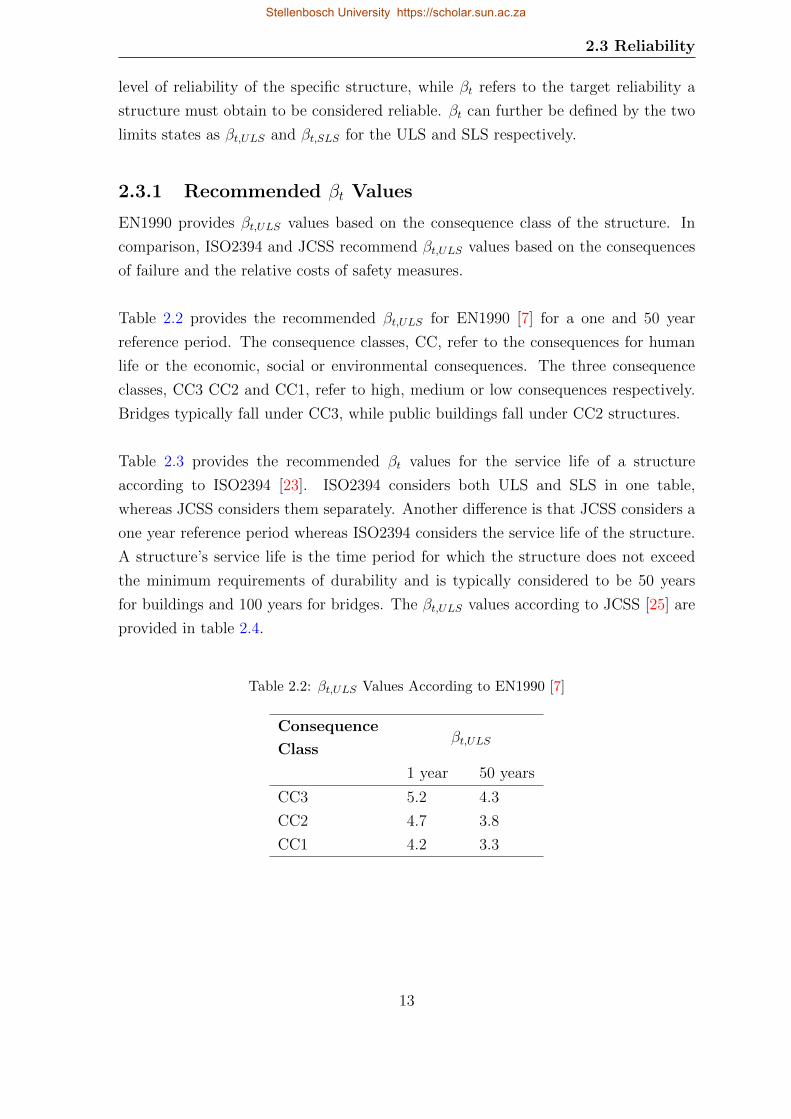
2.3.1 Recommended βt Values
EN1990 provides βt,ULS values based on the consequence class of the structure. In
comparison, ISO2394 and JCSS recommend βt,ULS values based on the consequences
of failure and the relative costs of safety measures.
Table 2.2 provides the recommended βt,ULS for EN1990 [7] for a one and 50 year
reference period. The consequence classes, CC, refer to the consequences for human
life or the economic, social or environmental consequences. The three consequence
classes, CC3 CC2 and CC1, refer to high, medium or low consequences respectively.
Bridges typically fall under CC3, while public buildings fall under CC2 structures.
Table 2.3 provides the recommended βt values for the service life of a structure
according to ISO2394 [23]. ISO2394 considers both ULS and SLS in one table,
whereas JCSS considers them separately. Another difference is that JCSS considers a
one year reference period whereas ISO2394 considers the service life of the structure.
A structure’s service life is the time period for which the structure does not exceed
the minimum requirements of durability and is typically considered to be 50 years
for buildings and 100 years for bridges. The βt,ULS values according to JCSS [25] are
provided in table 2.4.
Table 2.2: βt,ULS Values According to EN1990 [7]
Consequence
Classβt,ULS
1 year 50 years
CC3 5.2 4.3
CC2 4.7 3.8
CC1 4.2 3.3
13
Stellenbosch University https://scholar.sun.ac.za

2.3 Reliability
Table 2.3: βt Values According to ISO2394 [23] for the Service Life
Consequences of Failure
Relative Costs of
Safety MeasureSmall Some Moderate Great
High 0 1.5 2.3 3.1
Moderate 1.3 2.3 3.1 3.8
Low 2.3 3.1 3.8 4.3
Table 2.4: βt,ULS Values According to JCSS [25] for a One Year Reference Period
Relative Costs of
Safety Measure
Minor
Consequences
of Failure
Moderate
Consequences
of Failure
Large
Consequences
of Failure
High 3.1 3.3 3.7
Moderate 3.7 4.2 4.4
Low 4.2 4.4 4.7
For an irreversible SLS a βt,SLS = 1.5 and for the reversible SLS a βt,SLS = 0 is
accepted for the service life or a 50 year reference period [7, 23]. According to the
target βt,SLS values of ISO2394 (1998) [23], this corresponds to a high relative cost
of safety measure and small/some consequences of failure (table 2.3). EN1990 [7]
recommends for a one year reference period a βt,SLS = 2.9 which corresponds to the
same level of reliability as 1.5 for a 50 year reference period. JCSS [25] suggests βt,SLS
values for a one year reference period for different relative costs of safety measures.
Table 2.5 provides the values recommended in JCSS for irreversible SLS.
Table 2.5: βt,SLS Values According to JCSS [25] for a One Year Reference Period
Relative Cost of
Safety Measureβt,SLS
High 1.3
Normal 1.7
Low 2.3
14
Stellenbosch University https://scholar.sun.ac.za

2.3 Reliability
JCSS, ISO2394 and EN1990 provide recommendations for βt,ULS and βt,SLS based on
different reference periods. ISO2394 [23] recommends βt based on the expected service
life of the structure whereas JCSS [25] recommends βt for a 1 year and EN1990 [7] for
a 1 and 50 year reference period. EN1990 provides a relationship between a 1 year
reference period and an n year reference period, as shown in equation 2.7. Emphasis
must be placed on the fact that the reliability index for a reference period of one
year βt,1 has the same level of reliability as the corresponding target reliability index
βt,n [18].
βt,n = Φ−1([Φ(βt,1)]n) (2.7)
with βt,n Target reliability related to a n year reference period
βt,1 Target reliability related to a 1 year reference period
Φ Cumulative distribution function of
the standardized normal distribution
n Reference period
2.3.2 First Order Reliability Method, FORM
The First Order Reliability Method (FORM) is one of techniques available for the
reliability analysis of a structure. The FORM algorithm is discussed for the ULS in
this section, but the principle does not differ for the SLS.
Structural failure is defined as the inability of the structure or structural element to
satisfy the limit state (g(X) ≤ 0). Structural reliability is based on the relationship
between the random variables (X) of the limit state function.
As an example, R and E are assumed to be two normally distributed variables as
shown in figure 2.1 [13]. The design point P is defined at E = R. The safety margin
Z is the difference between the resistance and the load effect (equation 2.10). β is the
number of standard deviations σZ (equation 2.11) the safety margin Z is from zero.
The corresponding probability of failure is the probability that E is greater than R
(equation 2.8).
pf = P (E > R) = P (0 > Z) (2.8)
15
Stellenbosch University https://scholar.sun.ac.za

2.3 Reliability
µE µR
αEβσE αRβσR
P
X
f(x)
Figure 2.1: Normal distribution of E and R
To determine pf , a reliability analysis of the structure must be performed. For the
two uncorrelated normally distributed variables (shown in figure 2.1), β is found
using equation 2.9. The pf is then determined based on the relationship shown in
equation 2.6.
β =Z
σZ(2.9)
where:
Z = R− E (2.10)
σZ =√σ2R + σ2
E (2.11)
with β Reliability index
Z Safety margin
σZ Standard deviation of the safety margin
R Resistance
E Load effect
σR Standard deviation of the resistance
σE Standard deviation of the load effect
If the random variables are not normally distributed and/or the limit state is made
up of more than two variables, it is significantly more difficult to evaluate β in such
a simple form. FORM is considered to be one of the simplest and more efficient
reliability methods [5, 18]. In Handbook 2: Reliability Backgrounds [13] FORM is
16
Stellenbosch University https://scholar.sun.ac.za

2.3 Reliability
defined as:
“The approximate method of a given iterative algorithm that allows the reliability
index to be obtained by using a linear approximation to the limit state surface at the
point of minimum distance to the mean point of the variables.”
Or more simply FORM gives a linear algorithm to determine the value of β which is
the number of standard deviations the design point P is away from the mean. The
design point is where the most probable failure point or the line where the limit state
equation is g(X) = 0 [5, 13] and is shown in figures 2.1 and 2.2.
Figure 2.2: Design Point [7]
The limit state function or failure boundary is approximated by a tangent plane in
FORM [5]. Figure 2.2 shows this tangent plane along with the design point of the
limit state function of two random variables with transformed normal distributions
in a two-dimensional diagram. The sensitivity factors (αR and αE) are the direction
cosines of the normal failure boundary and are considered to be importance measures
of R and E in the FORM analysis [18]. The design values (coordinates of the design
point) are then determined using equations 2.12 and 2.13.
17
Stellenbosch University https://scholar.sun.ac.za

2.4 Concluding Remarks
Rd = µR − αRβσR (2.12)
Ed = µE − αEβσE (2.13)
Figure 2.3: FORM [18]
The main steps of FORM summarized in Holicky 2009 [18] are:
1. The basic variables, X, are transformed into standardized normal variables, U.
This is shown in figure 2.3.
2. If the failure boundary is not linear, the failure surface is approximated for a
given point.
3. Iteration is done until the design point is found.
4. β is determined, this is the number of standard deviations the mean value is
from the design point.
2.4 Concluding Remarks
This chapter summarises the key topics required to perform a reliability analysis.
The definition of the limit states is provided, which is later identified to be necessary
18
Stellenbosch University https://scholar.sun.ac.za
2.4 Concluding Remarks
in performing a reliability analysis. The model uncertainty was defined and the
available information regarding model factors related to typical SLS action-resistance
effects (for example crack widths or deflections) is provided. A definition of structural
reliability and the currently recommended values for βt are provided. Finally,
the FORM algorithm (identified as a suitable method for a reliability analysis) is
explained.
19
Stellenbosch University https://scholar.sun.ac.za
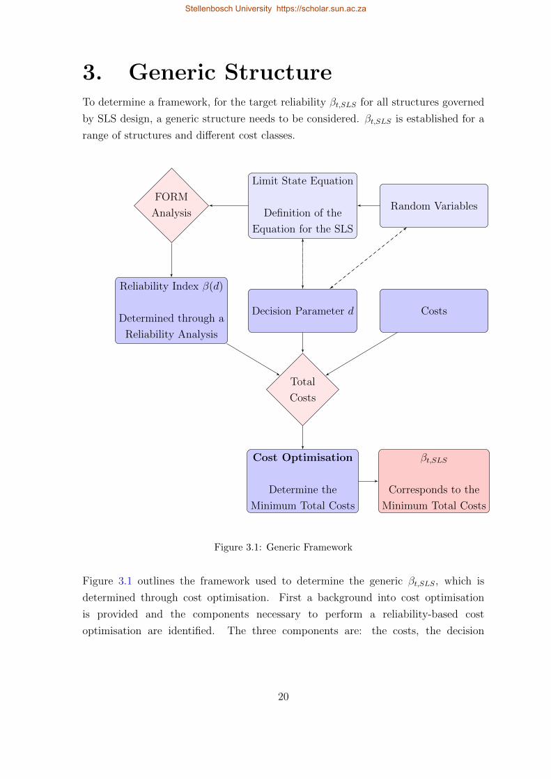
3. Generic StructureTo determine a framework, for the target reliability βt,SLS for all structures governed
by SLS design, a generic structure needs to be considered. βt,SLS is established for a
range of structures and different cost classes.
βt,SLS
Corresponds to the
Minimum Total Costs
Cost Optimisation
Determine the
Minimum Total Costs
Total
Costs
Decision Parameter d
Reliability Index β(d)
Determined through a
Reliability Analysis
Costs
FORM
Analysis
Limit State Equation
Definition of the
Equation for the SLS
Random Variables
Figure 3.1: Generic Framework
Figure 3.1 outlines the framework used to determine the generic βt,SLS, which is
determined through cost optimisation. First a background into cost optimisation
is provided and the components necessary to perform a reliability-based cost
optimisation are identified. The three components are: the costs, the decision
20
Stellenbosch University https://scholar.sun.ac.za

3.1 Cost Optimisation
parameter d and the reliability index β(d) which is a function of d. β(d) is related
to d through the limit state equation and the random variables of the limit state
equation. Once all the components are identified, cost optimisation is performed to
determine βt,SLS.
3.1 Cost Optimisation
In order for the structure to be viable from an economic point of view, a balance
between the consequences of failure and the costs of safety measures must be achieved.
Equation 3.1 [23] contains the total costs. The costs of safety measures include
costs which improve the structural reliability. In equation 3.1, the costs of safety
measures are defined as the building costs Cb and the maintenance costs Cm The
failure consequences include all costs relating to direct and indirect consequences [19,
46].
Ctot = Cb + Cm +∑
pf × Cf (3.1)
with Ctot The total costs
Cb The building or construction costs
Cm The expected maintenance costs
Cf The failure costs
pf Probability of failure
This balance is optimal when the total costs are at a minimum. The fundamental
principle of probabilistic optimization is to find the reliability level βt that would
minimize the total costs of the structure over its lifetime. To minimize the total
costs of the structure, the cost function needs to take into account some decision
parameter d. This is typically a vector of multiple decision parameters. Some of
the costs in equation 3.1 depend on d, which leads to equation 3.2. If d is a vector
of decision parameters,∑Cfpf (d) is the sum of all the expected costs of failures
associated with the different decision parameter.
The total costs of a structure Ctot as a function of the decision parameter is defined
in equation 3.2.
Ctot = C0 + C1d+∑
Cfpf (d) (3.2)
21
Stellenbosch University https://scholar.sun.ac.za
3.1 Cost Optimisation
with d Decision parameter(s)
C0 Initial costs independent of d
C1 Costs of providing safety; dependent on d
Cf Failure costs
pf (d) Probability of failure as a function of d
C0 + C1d Construction costs
Cfpf (d) Expected failure costs
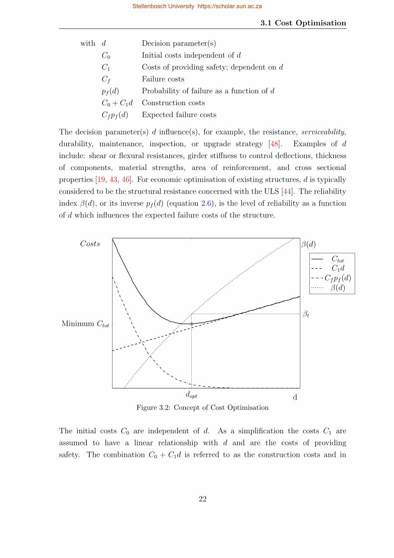
The decision parameter(s) d influence(s), for example, the resistance, serviceability,
durability, maintenance, inspection, or upgrade strategy [48]. Examples of d
include: shear or flexural resistances, girder stiffness to control deflections, thickness
of components, material strengths, area of reinforcement, and cross sectional
properties [19, 43, 46]. For economic optimisation of existing structures, d is typically
considered to be the structural resistance concerned with the ULS [44]. The reliability
index β(d), or its inverse pf (d) (equation 2.6), is the level of reliability as a function
of d which influences the expected failure costs of the structure.
Minimum Ctot
d
Costs
dopt
βt
β(d)
CtotC1d
Cfpf (d)β(d)
Figure 3.2: Concept of Cost Optimisation
The initial costs C0 are independent of d. As a simplification the costs C1 are
assumed to have a linear relationship with d and are the costs of providing
safety. The combination C0 + C1d is referred to as the construction costs and in
22
Stellenbosch University https://scholar.sun.ac.za
3.1 Cost Optimisation
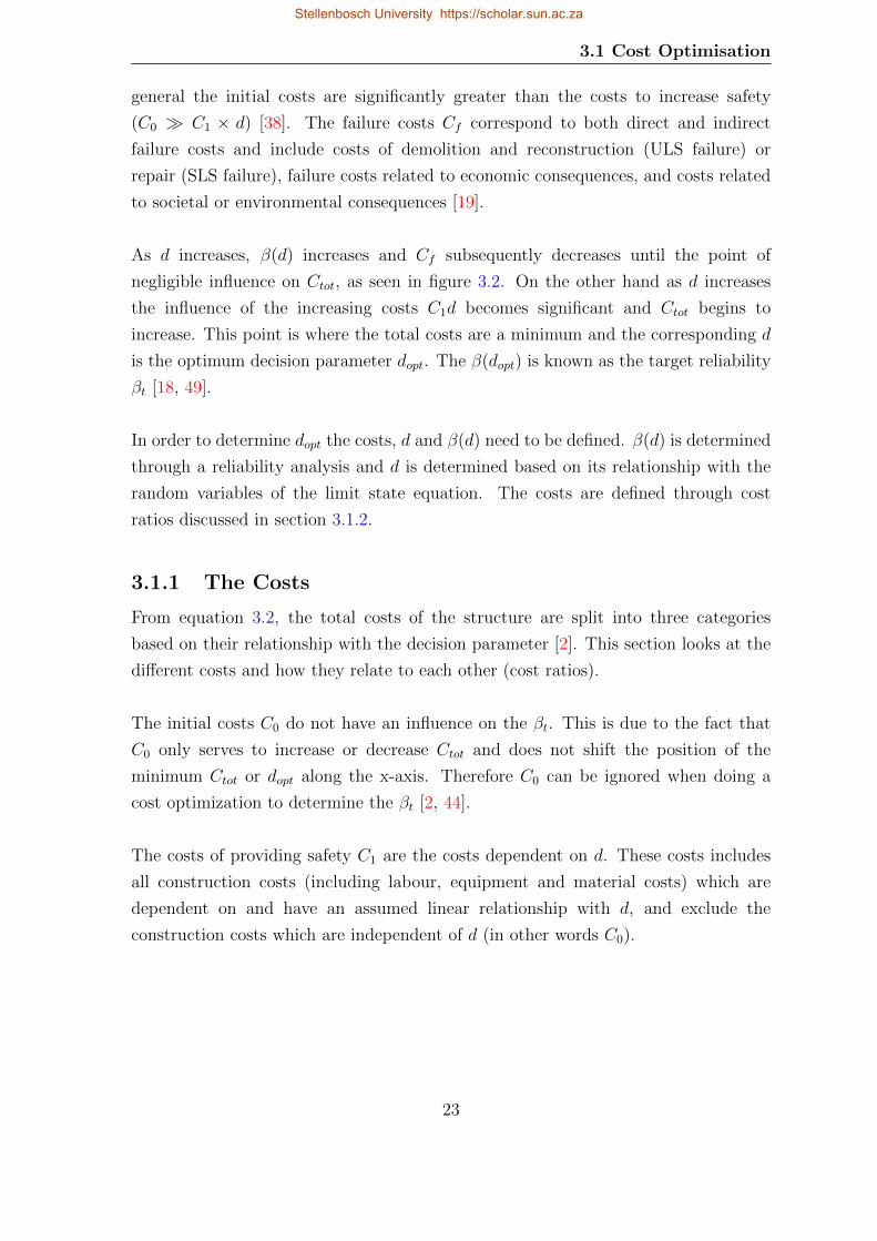
general the initial costs are significantly greater than the costs to increase safety
(C0 � C1 × d) [38]. The failure costs Cf correspond to both direct and indirect
failure costs and include costs of demolition and reconstruction (ULS failure) or
repair (SLS failure), failure costs related to economic consequences, and costs related
to societal or environmental consequences [19].
As d increases, β(d) increases and Cf subsequently decreases until the point of
negligible influence on Ctot, as seen in figure 3.2. On the other hand as d increases
the influence of the increasing costs C1d becomes significant and Ctot begins to
increase. This point is where the total costs are a minimum and the corresponding d
is the optimum decision parameter dopt. The β(dopt) is known as the target reliability
βt [18, 49].
In order to determine dopt the costs, d and β(d) need to be defined. β(d) is determined
through a reliability analysis and d is determined based on its relationship with the
random variables of the limit state equation. The costs are defined through cost
ratios discussed in section 3.1.2.
3.1.1 The Costs
From equation 3.2, the total costs of the structure are split into three categories
based on their relationship with the decision parameter [2]. This section looks at the
different costs and how they relate to each other (cost ratios).
The initial costs C0 do not have an influence on the βt. This is due to the fact that
C0 only serves to increase or decrease Ctot and does not shift the position of the
minimum Ctot or dopt along the x-axis. Therefore C0 can be ignored when doing a
cost optimization to determine the βt [2, 44].
The costs of providing safety C1 are the costs dependent on d. These costs includes
all construction costs (including labour, equipment and material costs) which are
dependent on and have an assumed linear relationship with d, and exclude the
construction costs which are independent of d (in other words C0).
23
Stellenbosch University https://scholar.sun.ac.za

3.1 Cost Optimisation
The failure costs Cf depend on the probability of failure as a function of the decision
parameter pf (d). The failure costs include: costs of repair (SLS failure), costs related
to economic losses, or costs related to societal and environmental consequences [43,
45]. The failure costs considered are those related to both direct and indirect failure
consequences. Determining the failure costs is the most important and often most
difficult step in cost optimization [19, 46]. The type of failure, in this case SLS
failure, will also play a role in determining Cf .
Serviceability failure is defined as the realisation of the action-resistance exceeding the
limiting design value. For example if the cracks in a structure are larger than the crack
width limit or the deflections are larger than the deflection limit. This is considered to
be SLS failure and results in a limited use of the structure and reduction of service life.
3.1.2 Cost Ratios
Due to the complexity in defining failure costs, specifically those related to the indirect
consequences, a cost ratio is utilised [1]. This cost ratio Cf/C1 is a ratio of the failure
consequences to the costs of providing safety (per unit of the decision parameter). A
relationship (cost ratio) between C1 and Cf is typically used when doing an economic
optimization as the exact costs of the structure are not known, and vary for different
structures. This ratio is obtained by setting the derivative of equation 3.2 with respect
to d equal to zero as shown in equation 3.4. Where the derivative is equal to zero,
dopt may be obtained.
∂Ctot∂d
= C1 + Cf∂pf (d)
∂d= 0 (3.3)
1 +CfC1
∂pf (d)
∂d= 0 (3.4)
While the βt,ULS recommended in JCSS were derived from a cost benefit analysis,
the βt,SLS were derived based on decision analysis and there is no clear link between
the above mentioned cost ratios and the SLS specifically for this class of special
structures [25]. Previously recommended or investigated ratios are discussed as a
guideline for determining ratios for the SLS. Cost ratios for the generic SLS are then
discussed.
24
Stellenbosch University https://scholar.sun.ac.za

3.1 Cost Optimisation
3.1.2.1 Cost Ratios Previously Investigated
Holicky [17] investigated the influence of the cost ratio, ranging from 1 to 106. For
the ULS, JCSS [25] defines the cost ratios by 3 consequence classes which can be
related to the consequence classes defined in EN1990 [16]. The ratio is defined as
ctot = Ctot/C1. The three consequence classes in JCSS [25] are minor, moderate and
large consequences of failure. Vrouwenvelder [50] defines these cost ratio for JCSS.
Sykora et al. [47] gives a range of cost ratios for the various consequence classes for
ULS. These ratios are shown in table 3.1.
Table 3.1: Cost Ratios for ULS
Consequence Class JCSS [25] Vrouwenvelder [50] Sykora et al. [47]
CC1 (minor) ctot < 2 Cf/C1 = 2 1 < Cf/C1 < 3
CC2 (moderate) 2 < ctot < 5 Cf/C1 = 4 5 < Cf/C1 < 20
CC3 (large) 5 < ctot < 10 Cf/C1 = 8 Cf/C1 > 20
3.1.2.2 Cost Ratios for the SLS
A parametric study of the cost ratios is performed to account for a range of
consequences of structural failure. The cost ratios from 0.5 up until 100 are
considered. The smaller ratios correspond to low costs of failure combined with high
costs of increasing safety. The higher ratios correspond to a combination of high
consequences of failure and low costs of increasing safety.
The cost ratios Cf/C1 are discussed based on their consequences. It is left to the
engineer’s judgement to determine the appropriate cost ratio for his/her specific
structure. The following descriptions are general guidelines to assist the engineer in
determining what reliability level said structure should have based on its construction
and failure costs.
Minor Consequences: Cf/C1 = [0.5, 0.8, 1.0]
These relatively small consequences occur when the failure costs are less than or equal
to the costs of providing safety. For example, SLS failure may result in relatively low
repair costs Cf compared to the costs of increasing safety C1 . These low failure costs
25
Stellenbosch University https://scholar.sun.ac.za

3.1 Cost Optimisation
typically correspond to minor repair costs with little to no indirect failure costs. It
is expected that if serviceability failure was to occur, the use of the structure would
not be drastically limited or affected and a small repair effort would easily rectify the
structure’s integrity.
For these cost ratios a relatively low βt,SLS is obtained as serviceability failure does not
result in large failure costs. The structural element under consideration might also be
an insignificant member of the structure, whose failure would not have a significant
impact on the structure’s integrity as a whole. Little effort is expected to achieve this
level of reliability as the failure consequences are considerably small or even negligible.
For a structure where Cf are significantly lower than C1, βt,SLS might also be
negative. When this is the case, ULS will govern the design of the structure and SLS
requirements will typically be easily fulfilled.
Moderate Consequences: Cf/C1= [1.5, 2.0, 4.0]
The failure costs for these consequences are slightly greater than the costs of
providing safety and more effort is required to achieve the required level of reliability
as the costs of failure now start to increase. These failure costs are related to a more
extensive repair effort as failure might result in a significant impact on the use of
the structure. The service life of the structure might also be shortened due to this
serviceability failure resulting in failure costs associated with the loss of usage of the
structure.
For this consequence class, there may be indirect failure costs (for example shortened
service life) that are greater than the costs of providing safety. It could also include
extensive repair costs which due to the nature of the repairs will cost more than the
initial costs of providing safety. For example, societal consequences may play a role
for an important water retaining structure or pre-stressed bridge.
Large Consequences: Cf/C1 = [10.0, 20.0, 50.0, 100.0]
This consequence class refers to a structure or a structural element where the failure
costs are significantly (10 or more times) greater than the costs of providing safety.
26
Stellenbosch University https://scholar.sun.ac.za

3.2 Reliability Analysis
For example this could be a relatively small element of the structure with relatively
cheap costs of providing safety. However, this is a critical element of the structure
and failure of this element will result in relatively large consequences of failure
with corresponding large failure costs. The direct and indirect failure costs of this
element may be significantly larger than the costs of providing safety of this small,
critical element. Failure of this element might result in replacing the element and
the indirect costs associated with the immediate disuse (temporary or permanent) of
the structure for the replacement of the structural element are relatively expensive
compared to the initial costs in the construction phase.
3.2 Reliability Analysis
A reliability analysis is performed to obtain the β(d) values from the defined limit
state function for the SLS.
3.2.1 The Limit State Function
The general SLS equation defined in EN1990 is shown in equation 3.5 [7]. For the
SLS, structural failure is defined as the occurrence of the action-resistance effect
E exceeding the limiting design value L (E > L). E is the random variable
that is influenced by the loading but also takes the resistance of the structure into
account. For example, the mean value prediction of the maximum deflection δm,max is
determined from the load effect (action) in combination with the material properties
(resistance).
g(L,E) = L− E = 0 (3.5)
with L Limiting design value
E Action-resistance effect
To perform a first order reliability method (FORM) analysis of equation 3.5, the
variables, L and E, need to be assigned values in the generic sense. As L is typically a
prescribed limit (for example the crack width limit for cracking or the deflection limit
for deflections) it is assumed to be a deterministic value. Based on this assumption,
the SLS can be simplified to equation 3.7 by dividing equation 3.5 by L (shown in
equation 3.6).
27
Stellenbosch University https://scholar.sun.ac.za

3.2 Reliability Analysis
Dividing by L:
g(L,E) =L
L− E
L= 0 (3.6)
If L is deterministic then:
g(1, E) = 1− ηE = 0 (3.7)
with E SLS action-resistance effect
η Factor which is equal to 1/L
The range for the factor η includes includes the limiting design values for all SLS
scenarios for example crack widths and deflections. For crack widths, the limiting
design value is a prescribed value in the range of 0.1 - 1 mm. This results in η values
of greater than or equal to one (η ≥ 1). Conversely for deflections, the limiting
design value is typically prescribed by the ratio of span over depth or span over 250.
As these values are typically larger than one, the resulting η values are less than one
(η < 1). However, η is always greater than zero (η > 0) as all serviceability limiting
design values are assumed to be positive.
Due to the large range of η, it is suitable to assume η = 1 for the generic case. The
action-resistance effect E is then defined for L = 1 in the generalised sense. E is
defined in equation 3.8 as the product of the predicted action-resistance effect Y and
the model factor θ.
E = θY (3.8)
with θ The model uncertainty
Y The predicted action-resistance effect
θ takes into account all uncertainty associated with the mathematical simplifications
used to model physical behaviour by taking into account the statistical differences
between the predicted and measured values [10, 20, 36]. Y is the predicted
action-resistance effect prescribed by a prediction model (for example in a national
standard). For example, it is the mean value prediction of the maximum crack width
wm,max for cracking or the mean value prediction of the maximum deflection δm,max.
28
Stellenbosch University https://scholar.sun.ac.za

3.2 Reliability Analysis
Y is random variable typically found through an equation. For example, the crack
width equation which comprises of the random variables of both the action effect
(loading) and the resistance (material strengths). For consistency, θ must relate the
experimental results to the same prediction model used to calculate Y [20].
3.2.1.1 The Mean Value of the Action-Resistance Effect µE
It is necessary to assess the reliability index β(d) in terms of the decision parameter
d. This is done by finding a relationship between d and the random variables of the
limit state equation. Typically d adjusts the resistance rather than load for the ULS.
This establishes a relationship between the resistance and d. However, for the SLS
E is the variable (for example crack widths, deflections, stresses, or vibrations) that
is affected by both the action and resistance. A relationship between the mean value
of the action-resistance effect µE and d needs to be established.
Rackwitz [38] defined a generic decision parameter for the ULS based on the ratio of
the mean values of the load effect and the resistance. For the SLS, this can be rewritten
as the ratio of the limiting design value µL and mean value of the action-resistance
effect µE. Equation 3.9 shows the relationship used by Rackwitz which is simplified
based on the generalised limit state function for the SLS.
d =L
µE=
1
ηµE(3.9)
where
µE = µθµY (3.10)
with L Deterministic limiting design value
µE Mean value of the action-resistance effect
µθ Mean value of the model uncertainty
µY Mean value of the predicted action-resistance effect
From equation 3.9, d is the generic decision parameter that includes any number
of physical parameters. These parameters are structural design properties and
choices on the SLS performance of the element under consideration. By increasing
or changing these parameters, the SLS performance of the element improves. In
29
Stellenbosch University https://scholar.sun.ac.za

3.2 Reliability Analysis
other words, d is related to the distance between µE and 1. As d increases, the
distance between µE and 1 decreases resulting in a smaller pf (d). This is illustrated
in figure 3.4.
As failure is likely to occur when d < 1 (g < 0), the range for the decision parameters
is chosen to take into account the scenarios where failure is more likely (d < 1) and
increases until the probability of failure is small (d = 3). This range (d = [0.9 − 3])
is evaluated in increments of ∆d = 0.01. The small increments are necessary to
observe the influence in the change of β(d) on the total costs, specifically for a small
coefficient of variation VE as explained in section 3.3.2.
3.2.2 Generic β(d) Values
Based on the relationship between the decision parameter and the action-resistance
effect, a FORM analysis is performed on the generic limit state function (equation 3.7)
to determine β(d). The coefficient of variation VE is a measure of the relative
variability of structural behaviour. To account for different structures, VE is
considered to range parametrically. The range considered is VE = [0.05 − 0.50] in
increments of ∆VE = 0.05. A summary of the variables for the FORM analysis of
equation 3.7 is shown in table 3.2. The software, Risk Tools (RT) [41], is used for the
FORM analysis.
Table 3.2: Range of Variables Considered in the Generic Reliability Analysis
Variable Minimum Maximum Increments
Decision Parameter d 0.90 3.00 0.01
Action-Resistance Effect µE 0.33 1.11 1/d
VE 0.05 0.50 0.05
The action-resistance effect E is assumed to have a lognormal (LN) distribution
and is scaled by η = 1. A LN distribution is chosen as it has a lower bound at
zero with a positive skewness and is typically used to describe some loads, material
strengths and geometrical data [13]. Most model factors are also assumed to have a
LN distribution. A LN distribution is, therefore, deemed suitable to cover the SLS
action-resistance effect. This assumption is later verified through the examples in
30
Stellenbosch University https://scholar.sun.ac.za

3.2 Reliability Analysis
chapters 4 and 5.
The β(d) values are related to a one year reference period. Holicky [15] states
that the reference period is associated with the period of time corresponding to the
statistical assessment of the time variance of the random variables and not with the
design working life. It is suitable to determine βt,SLS based on a one year reference
period. This is supported by Rackwitz [38] by stating:
“The optimal solution for building facilities with or without a systematic rebuilding
policy is based on failure intensities and not on time-dependent failure probabilities.”
The parametrically varied d and subsequently µE in determining β(d) is essential for
an economic optimisation to determine βt,SLS. For each VE a corresponding βt,SLS is
determined corresponding to dopt where the costs are a minimum. Figure 3.3 shows
the influence of VE and d on the reliability index β(d). β(d) is directly proportional
to d and inversely proportional to VE.
1.0 1.2 1.4 1.6 1.8 2.0 2.2 2.4 2.6 2.8 3.0
0.0
1.0
2.0
3.0
4.0
d
β(d) VE:0.050.100.150.200.250.300.350.400.450.50
Figure 3.3: Generic β(d)
The first observation made from figure 3.3 is that as d increases β(d) increases as
illustrated figure 3.4 where an increase in d results in a decrease in pf (d). Figure 3.4a
31
Stellenbosch University https://scholar.sun.ac.za

3.2 Reliability Analysis
illustrates the case for E > L which results in a low β(d), this case refers to
non-typical design scenarios. Figure 3.4b illustrates the case where E = L, and
results in β(d) ≈ 0. This corresponds to the current recommended βt,SLS for the
irreversible SLS. Finally, figure 3.4c illustrates typical design scenarios where E < L.
As d increases, E decreases resulting in larger β(d) values.
The second set of observations made is on the influence of VE as illustrated in
figure 3.5. For a low VE, the obtained β(d) values are high and as VE increases the
β(d) values decrease, this is considered to be the normal trend of the influence of VE.
This trend is intuitive as the more uncertain the design, the less reliable the structure
is, in other words there is a higher probability of failure. It can be seen that for the
range of VE a large range of β(d) values are accounted for.
L E
(a) d < 1
E = L
(b) d = 1
E Lpf
(c) d > 1
� pf
Figure 3.4: Relationship Between E and L as d Varies
32
Stellenbosch University https://scholar.sun.ac.za

3.2 Reliability Analysis
E L
VE0.500.300.10
� pfFigure 3.5: Influence of VE on pf
However, there is a discontinuity in the trend of β(d) values for d ≤ 1 (E ≥ L). This
is seen clearly in figure 3.6. At E ≈ L, the β(d) values are all approximately equal
and before there is very little difference between the obtained β(d) values. However
for E ≥ L, the lower VE the lower the β(d) value is which is inverse to what occurs
when g > 0. This is further explained using figure 3.5 where the failure region is
larger for a small VE and smaller for a large VE when d ≤ 1.
1.0 1.2 1.4 1.6 1.8 2.0 2.2 2.4 2.6 2.8 3.0
0.0
1.0
2.0
3.0
4.0
d
β(d) VE:0.050.100.150.200.250.300.350.400.450.50
0.90 0.95 1.00 1.05 1.10
−0.40
−0.20
0.00
0.20
0.40
Figure 3.6: Change in β(d) at d ≈ 1
33
Stellenbosch University https://scholar.sun.ac.za

3.3 Target Reliability for SLS
3.3 Target Reliability for SLS
From the range of Cf/C1 determined in chapter 3.1 and the β(d) values for the
range of VE determined in chapter 3.2, a parametric table of the target reliability
for concrete structures can be established through economic optimisation. This
parametric table takes into account a range of costs and consequence classes while
suitably covering all concrete structures (both new and existing) for the SLS (both
typical structures and those governed by SLS design).
3.3.1 Cost Optimisation
On the basis of the generalised β(d) values, a cost optimisation is performed for the
range of cost ratios Cf/C1. For each combination of Cf/C1 and VE, the minimum
total cost and corresponding dopt is determined using equation 3.2. βt,SLS is taken as
β(dopt) and is summarised in table 3.3. The results from the cost optimisation (Ctot
versus d) for the parametrically varied VE and Cf/C1 are shown in figures 3.7 and 3.8
respectively. These figures are discussed in more detail in the following paragraphs.
Figure 3.7 portrays the influence of Cf/C1 on Ctot for the different values of VE. See
Appendix A figures A.1 to A.10 for the larger figures. The β(d) corresponding to VE
is shown on the secondary axis. It can be seen that the optimal decision parameter
dopt (where the minimum total costs occur) is dependent on both VE and Cf/C1.
For larger values of d (d > dopt), Ctot is independent of the expected failure costs.
This is due to the increased negligible influence of β(d) on Cf and the increased cost
of providing safety C1d. In other words for these large values of d the structure is so
safe that pf approaches zero and Ctot approaches the construction costs (C0 + C1d).
However, for smaller values of d (d < dopt), Ctot varies as Cf/C1 varies.
The change of magnitude in dopt for different VE’s also increases as the cost ratio
increases. For a low Cf/C1, the minimum total costs occur for a small d as the
influence of β(d) becomes negligible compared to the costs to improve the reliability
versus the small consequences of failure. Whereas for a larger cost ratio, where the
expected consequences become more significant, the influence of β(d) becomes larger
and the position of dopt varies more significantly.
34
Stellenbosch University https://scholar.sun.ac.za

3.3 Target Reliability for SLS
Figure 3.8 portrays the influence of VE on Ctot for different values of Cf/C1. See
Appendix A figures A.20 to A.11 for the full figures. For a specific cost ratio, it
can be observed that a lower VE results in a lower minimum total costs and smaller
corresponding dopt compared to those of a higher VE. However, the corresponding
β(dopt) is higher for a low VE than for a high VE. This is also illustrated using figure 3.5.
Figure 3.8e clearly shows the influence of the change in β(d) at d ≈ 1 is apparent
even when considering Ctot. The general trend is for Ctot to be greater for a higher
VE and decrease as VE decreases. However, the inverse of this trend occurs for d < 1
where Ctot is greater for a lower VE. This corresponds to the pivot point identified for
the β(d) values as shown in figure 3.6. This change in Ctot occurs for all cost ratios,
but is most apparent on figure 3.8e. For figures 3.8a to 3.8d this pivot in total costs
occurs for Ctot > 5 and exceeds the range of the graph as shown. This inverse in the
trend does not typically correspond to design scenarios as E > L.
The influence of VE through β(d) on the total costs is apparent in both figures 3.7
and 3.8. This is because the pf (d) region (E > L) is dependent on VE. This is shown
in figure 3.5 where the pf for a low VE is small compared to that of a high VE. For a
low VE there is a corresponding small variability on Ctot. Conversely for a higher VE
the corresponding variability on Ctot is greater.
In terms of βt,SLS this trend of increasing variability of Ctot as VE increases is
identified to have an influence on position of dopt rather than variability βt,SLS. The
corresponding βt,SLS decreases as VE decreases. This is due to the corresponding
β(d) which varies as VE varies. From this it can be concluded that the influence of
VE on the total costs is based on the influence of VE on β(d).
For figures 3.7i and 3.7j, the total costs are not calculated for the entire range of
d. This is due to the fact that for such small VE’s, β(d) rapidly increases to such a
high level of reliability. This results in a negligible pf (pf ≈ 0) for larger values of
d. This negligible pf is clearly illustrated for the low VE in figure 3.5. However, Ctot
does increase resulting in a reasonable βt,SLS which is not observed at the end of the
calculated β(d) values.
35
Stellenbosch University https://scholar.sun.ac.za

3.3 Target Reliability for SLS
1.0 1.5 2.0 2.5 3.01.0
2.0
3.0
4.0
5.0
d
Ctot
0.0
2.0
4.0β(d)
(a) VE = 0.50
1.0 1.5 2.0 2.5 3.01.0
2.0
3.0
4.0
5.0
d
Ctot
0.0
2.0
4.0β(d)
(b) VE = 0.45
1.0 1.5 2.0 2.5 3.01.0
2.0
3.0
4.0
5.0
d
Ctot
0.0
2.0
4.0β(d)
(c) VE = 0.40
1.0 1.5 2.0 2.5 3.01.0
2.0
3.0
4.0
5.0
d
Ctot
0.0
2.0
4.0β(d)
(d) VE = 0.35
1.0 1.5 2.0 2.5 3.01.0
2.0
3.0
4.0
5.0
d
Ctot
0.0
2.0
4.0β(d)
(e) VE = 0.30
1.0 1.5 2.0 2.5 3.01.0
2.0
3.0
4.0
5.0
d
Ctot
0.0
2.0
4.0β(d)
(f) VE = 0.25
1.0 1.5 2.0 2.5 3.01.0
2.0
3.0
4.0
5.0
d
Ctot
0.0
2.0
4.0β(d)
(g) VE = 0.20
1.0 1.5 2.0 2.5 3.01.0
2.0
3.0
4.0
5.0
d
Ctot
0.0
2.0
4.0β(d)
(h) VE = 0.15
1.0 1.5 2.0 2.5 3.01.0
2.0
3.0
4.0
5.0
d
Ctot
0.0
2.0
4.0β(d)
(i) VE = 0.10
1.0 1.5 2.0 2.5 3.01.0
2.0
3.0
4.0
5.0
d
Ctot Cf/C1
1005020104.02.01.51.00.80.5
0.0
2.0
4.0β(d)
(j) VE = 0.05
Figure 3.7: Influence of Cf/C1 on the Total Costs for Different Values of VE
36
Stellenbosch University https://scholar.sun.ac.za

3.3 Target Reliability for SLS
1.0 1.5 2.0 2.5 3.01.0
2.0
3.0
4.0
5.0
d
Ctot
(a) Cf/C1 = 100
1.0 1.5 2.0 2.5 3.01.0
2.0
3.0
4.0
5.0
d
Ctot
(b) Cf/C1 = 50
1.0 1.5 2.0 2.5 3.01.0
2.0
3.0
4.0
5.0
d
Ctot
(c) Cf/C1 = 20
1.0 1.5 2.0 2.5 3.01.0
2.0
3.0
4.0
5.0
d
Ctot
(d) Cf/C1 = 10
1.0 1.5 2.0 2.5 3.01.0
2.0
3.0
4.0
5.0
d
Ctot
(e) Cf/C1 = 4.0
1.0 1.5 2.0 2.5 3.01.0
2.0
3.0
4.0
5.0
d
Ctot
(f) Cf/C1 = 2.0
1.0 1.5 2.0 2.5 3.01.0
2.0
3.0
4.0
5.0
d
Ctot
(g) Cf/C1 = 1.5
1.0 1.5 2.0 2.5 3.01.0
2.0
3.0
4.0
5.0
d
Ctot
(h) Cf/C1 = 1.0
1.0 1.5 2.0 2.5 3.01.0
2.0
3.0
4.0
5.0
d
Ctot
(i) Cf/C1 = 0.8
1.0 1.5 2.0 2.5 3.01.0
2.0
3.0
4.0
5.0
d
Ctot VE0.500.450.400.350.300.250.200.150.100.05
(j) Cf/C1 = 0.5
Figure 3.8: Influence of VE on the Total Costs for Different Values of Cf/C1
37
Stellenbosch University https://scholar.sun.ac.za

3.3 Target Reliability for SLS
3.3.2 Influence of the Increment of d
In section 3.2.1 the increment of d was chosen to be ∆d = 0.01. The reason for a
small increment is based on the steeper slope of β(d) as a result of low VE’s. A small
investigation into βt,SLS was conducted for the range VE = [0.05− 0.2] for ∆d = 0.01,
0.05, and 0.10. Figure 3.9 shows the influence of ∆d for the range of Cf/C1 on βt,SLS.
0 10 20 30 40 50 60 70 80 90 1000.0
1.0
2.0
3.0
4.0
Cf/C1
βt,SLS
(a) Cf/C1 = 0.5− 100
0 2 4 6 8 100.0
1.0
2.0
3.0
4.0
Cf/C1
βt,SLS VE∆d = 0.01 ∆d = 0.05 ∆d = 0.10
0.05 0.05 0.050.10 0.10 0.100.15 0.15 0.150.20 0.20 0.20
(b) Cf/C1 = 0.5− 10
Figure 3.9: Influence of ∆d
The smaller ∆d results in a change of βt,SLS as the cost ratio increases, compared to
the larger ∆d where there is little to no change in βt,SLS. This is because for a small
VE, dopt is sharply defined due to the steep slope of β(d). These large increments in
β(d) over d result in inaccurate estimates of β(dopt). This inaccuracy in estimating
β(dopt) is clear especially for VE = 0.05, whereas from VE ≥ 0.15 the influence of ∆d
becomes negligible. However, the difference in βt,SLS for VE = 0.05 or 0.10 clearly
38
Stellenbosch University https://scholar.sun.ac.za
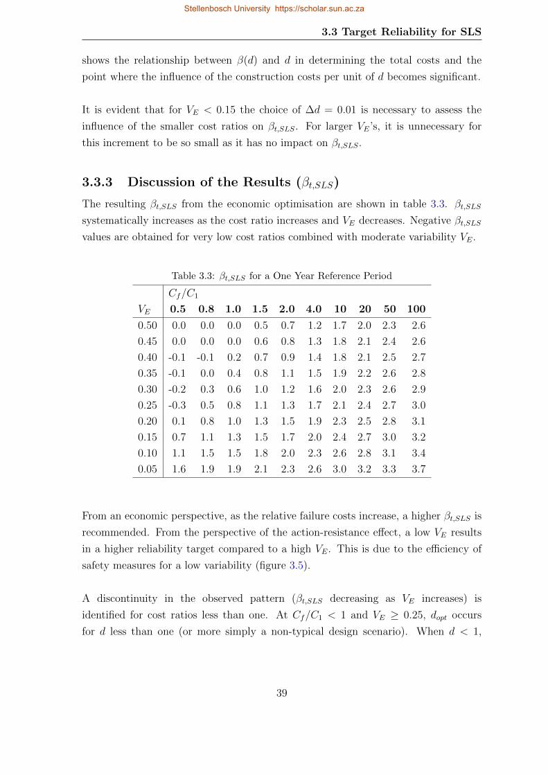
3.3 Target Reliability for SLS
shows the relationship between β(d) and d in determining the total costs and the
point where the influence of the construction costs per unit of d becomes significant.
It is evident that for VE < 0.15 the choice of ∆d = 0.01 is necessary to assess the
influence of the smaller cost ratios on βt,SLS. For larger VE’s, it is unnecessary for
this increment to be so small as it has no impact on βt,SLS.
3.3.3 Discussion of the Results (βt,SLS)
The resulting βt,SLS from the economic optimisation are shown in table 3.3. βt,SLS
systematically increases as the cost ratio increases and VE decreases. Negative βt,SLS
values are obtained for very low cost ratios combined with moderate variability VE.
Table 3.3: βt,SLS for a One Year Reference Period
Cf/C1
VE 0.5 0.8 1.0 1.5 2.0 4.0 10 20 50 100
0.50 0.0 0.0 0.0 0.5 0.7 1.2 1.7 2.0 2.3 2.6
0.45 0.0 0.0 0.0 0.6 0.8 1.3 1.8 2.1 2.4 2.6
0.40 -0.1 -0.1 0.2 0.7 0.9 1.4 1.8 2.1 2.5 2.7
0.35 -0.1 0.0 0.4 0.8 1.1 1.5 1.9 2.2 2.6 2.8
0.30 -0.2 0.3 0.6 1.0 1.2 1.6 2.0 2.3 2.6 2.9
0.25 -0.3 0.5 0.8 1.1 1.3 1.7 2.1 2.4 2.7 3.0
0.20 0.1 0.8 1.0 1.3 1.5 1.9 2.3 2.5 2.8 3.1
0.15 0.7 1.1 1.3 1.5 1.7 2.0 2.4 2.7 3.0 3.2
0.10 1.1 1.5 1.5 1.8 2.0 2.3 2.6 2.8 3.1 3.4
0.05 1.6 1.9 1.9 2.1 2.3 2.6 3.0 3.2 3.3 3.7
From an economic perspective, as the relative failure costs increase, a higher βt,SLS is
recommended. From the perspective of the action-resistance effect, a low VE results
in a higher reliability target compared to a high VE. This is due to the efficiency of
safety measures for a low variability (figure 3.5).
A discontinuity in the observed pattern (βt,SLS decreasing as VE increases) is
identified for cost ratios less than one. At Cf/C1 < 1 and VE ≥ 0.25, dopt occurs
for d less than one (or more simply a non-typical design scenario). When d < 1,
39
Stellenbosch University https://scholar.sun.ac.za

3.4 Concluding Remarks
the inverse in the normal trend for β(d) occurs. In other words, a high VE results
in greater β(d) than for a lower VE, as shown in figure 3.3. For Cf/C1 < 1, this
pivot in the trend of β(d) values and the relatively low value of dopt results in the
discontinuity of βt,SLS. Therefore, for Cf/C1 < 1 a high VE results in a βt,SLS value
which is higher than the resulting βt,SLS for a medium VE.
The high target values correspond to high cost ratios or high consequences of failure
that are typically associated with ULS failure. For example βt,SLS = 3.7 shown in
table 3.3 corresponds to the βt,ULS recommendation in JCSS [25] (table 2.4) for high
or moderate costs of safety measures corresponding to large or minor consequences
of failure respectively. However, for design situations where SLS failure may have
severe consequences (for example environmental contamination due to leakage of a
hazardous liquid retaining structure) or where the costs of improving safety is low,
these values may also be appropriate for SLS design. Another example of severe
failure consequence due to SLS failure is the functionality requirements of hospitals
and also all buildings expected to function after in emergency operations would have
significant failure costs [28].
The low VE’s are expected to correspond to SLS design situations that are governed
by deflection or stress requirements, with an presumably small variability. Conversely
the higher VE’s are expected to correspond for example to cracking, where model
uncertainty is known to be high [30, 31].
Table 3.3 demonstrates that optimal reliability is lower for design situations with
higher variability than for lower variability, given a similar cost ratio. This would
imply optimal (target) reliability should be lower for SLS design situations that are
characterised by high variability, such as crack width predictions, compared to design
situations characterised by lower variability such as stresses or deflections. This
is because high uncertainty reduces the effect of moderate safety measures (figure 3.5).
3.4 Concluding Remarks
This chapter develops and implements a generic framework for determining βt,SLS.
First, the principle of economic optimisation (used to determine βt,SLS) is discussed
and the components required to perform a cost optimisation are identified. The two
40
Stellenbosch University https://scholar.sun.ac.za

3.4 Concluding Remarks
cost components are the failure costs Cf and the costs of providing safety C1. A range
of cost and consequence classes are accounted for by the range Cf/C1 = [0.5 − 100].
The limit state equation is generalised as a basis for a reliability analysis. From the
generic limit equation, a relationship between the action-resistance effect and the
decision parameter is defined. A range of structures is accounted for by the range
VE = [0.05− 0.5]. A FORM analysis of the generic limit state equation is performed
to determine β(d). Finally cost optimisation is used to determine βt,SLS.
βt,SLS is determined parametrically accounting for a range of structures and a range
of cost classes. Table 3.3 covers a large range of structures for a range of serviceability
conditions in a generic sense. For a specific structure, the generic framework can
be applied to determine βt,SLS and chapters 4 and 5 provide such example applications.
41
Stellenbosch University https://scholar.sun.ac.za
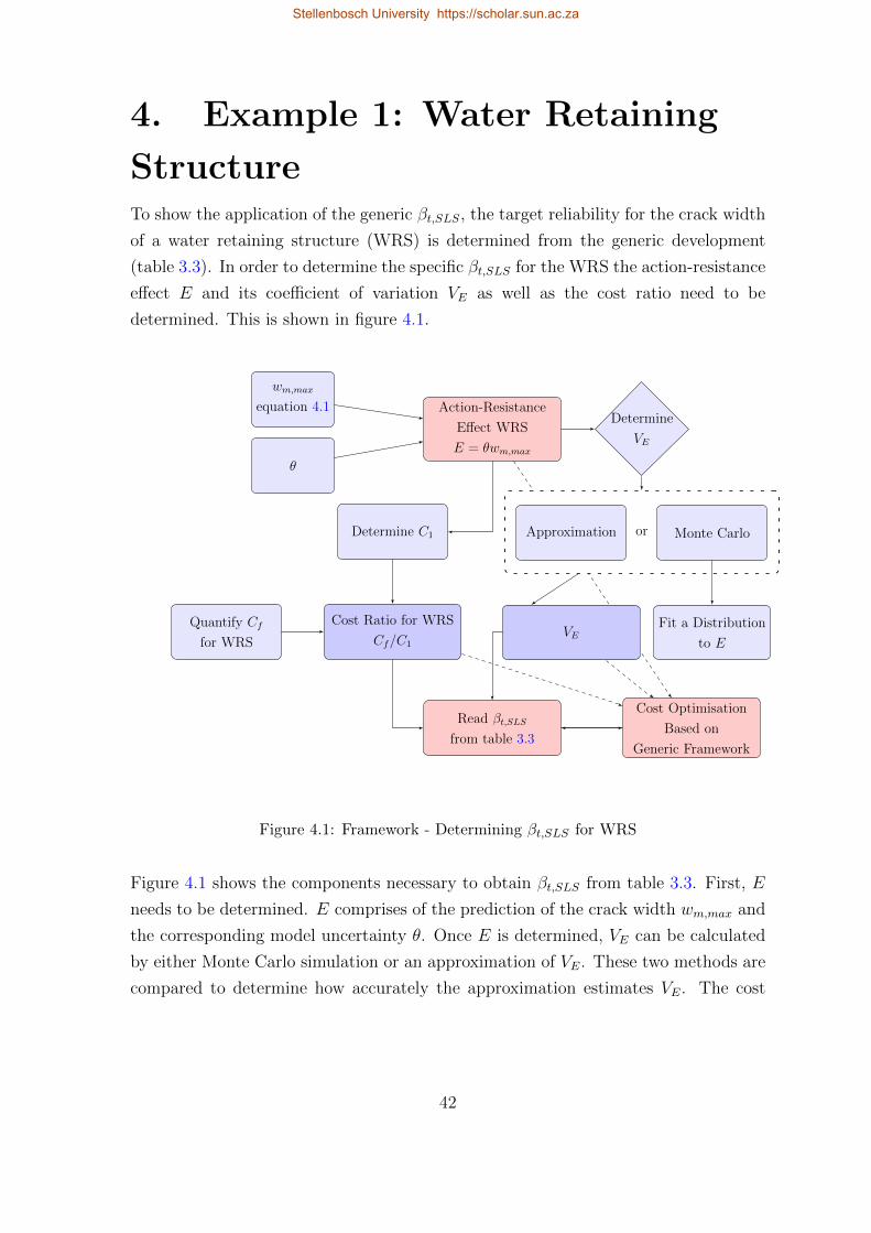
4. Example 1: Water Retaining
StructureTo show the application of the generic βt,SLS, the target reliability for the crack width
of a water retaining structure (WRS) is determined from the generic development
(table 3.3). In order to determine the specific βt,SLS for the WRS the action-resistance
effect E and its coefficient of variation VE as well as the cost ratio need to be
determined. This is shown in figure 4.1.
Action-Resistance
Effect WRS
E = θwm,max
Determine C1
Cost Ratio for WRS
Cf/C1
Quantify Cf
for WRS
Determine
VE
orApproximation Monte Carlo
Fit a Distribution
to EVE
Read βt,SLS
from table 3.3
Cost Optimisation
Based on
Generic Framework
wm,max
equation 4.1
θ
Figure 4.1: Framework - Determining βt,SLS for WRS
Figure 4.1 shows the components necessary to obtain βt,SLS from table 3.3. First, E
needs to be determined. E comprises of the prediction of the crack width wm,max and
the corresponding model uncertainty θ. Once E is determined, VE can be calculated
by either Monte Carlo simulation or an approximation of VE. These two methods are
compared to determine how accurately the approximation estimates VE. The cost
42
Stellenbosch University https://scholar.sun.ac.za

4.1 Action-Resistance Effect
ratio is the other component of the generic table of βt,SLS values. This is determined
by specifically quantifying the failure costs Cf and the costs of providing safety C1.
As shown in figure 4.1, there is a link between E and C1. Once VE and Cf/C1 are
quantified for this specific WRS, βt,SLS is obtained from table 3.3.
To demonstrate how the βt,SLS from the generic structure would compare to the
specific structure, cost optimisation is performed. The specific costs and statistical
properties of the WRS are used. The results from the cost optimisation are compared
to βt,SLS read from the table.
4.1 Action-Resistance Effect
From the generalised limit state equation (equation 3.7) the action-resistance effect
is defined as E = θY (equation 3.8). The model uncertainty θ for the crack width
prediction model of the Eurocode is discussed in section 4.1.2. For cracking the
predicted serviceability condition Y is the mean value prediction of the maximum
(mean-maximum) crack width wm,max of the WRS. wm,max is based on the Eurocode
as discussed in section 4.1.1.
Two circular water retaining structures (WRS) are considered for both flexural
and tensile crack widths according to the specifications of the Eurocodes.
EN1992 Part 3 [9] deals with WRS. Limitations on the crack width prediction
of the structure typically govern the design of WRS. Although the SLS governs the
design, the structure must still be checked to ensure that ULS requirements are
met. It is assumed that the ULS requirements are met and serviceability governs the
design as the focus of this study is to determine βt,SLS.
4.1.1 Crack Width Equation
The mean-maximum crack width for the WRS is calculated based on the prediction
model of the Eurocode. EN1992-1-3 [9] stipulates the provisions for retaining
structures and the crack width equation is found in EN1992-1-1 [8]. As a reliability
analysis is based on a mean value prediction, wm,max is calculated from the mean
values of the random variables which the crack width equation consists of. wm,max
is calculated using equation 4.1, which follows the provisions of section 7.3.4 in
43
Stellenbosch University https://scholar.sun.ac.za

4.1 Action-Resistance Effect
EN1992-1-1 [8].
wm,max = srm,max(εsm − εcm) (4.1)
with srm,max Maximum crack spacing (equation 4.4).
εsm Steel strain (equation 4.2).
εcm Concrete strain (equation 4.3).
The crack width is the mean-maximum crack spacing srm,max multiplied by the
difference between the mean strain in the steel εsm and the mean strain in the concrete
εcm. The strains in the steel and concrete are determined by equations 4.2 and 4.3
respectively. The difference between the strains must be greater than 0.6σs/Es.
However, as the reliability analysis is based on the mean value prediction and not
the design value the crack width prediction in this chapter ignores the limits on the
design. srm,max is calculated by using equation 4.4 and is a mean value prediction of
the maximum crack spacing.
εsm =σsEs
(4.2)
εcm =kt
fctmρp,eff
(1 + αeρp,eff )
Es(4.3)
srm,max = k3c+ k4k1k2φ
ρp,eff(4.4)
with Es Elastic modulus of steel.
σs Stress in tension reinforcement, assuming a cracked section.
σs = Ms
zAsor σs = Ts
As
kt The factor dependent on the load duration. See table 4.1.
fctm Mean value of the tensile concrete strength.
ρp,eff Ratio of (As + ξ1Ap)/Ac,eff .
As Area of reinforcing steel.
Ap Area of pre- or post tensioned tendons.
Ac,eff Effective area of concrete surrounding the reinforcement in tension.
ξ1 Adjusted ratio of the bond strength.
44
Stellenbosch University https://scholar.sun.ac.za

4.1 Action-Resistance Effect
αe Ratio of Es/Ecm.
Ecm Concrete modulus.
c Concrete cover.
φ The bar diameter.
k1 The factor taking the bond properties into account. See table 4.1.
k2 The factor taking the distribution of strain into account. See table 4.1.
k3 See table 4.1.
k4 See table 4.1.
For ρp,eff , As is the area of steel reinforcement, and Ap is the area of prestressing
tendons. If there are no prestressing tendons in the structure Ap = 0. Ac,eff is the
effective depth in tension hc,eff multiplied by the width b. The effective depth hc,eff
is the minimum of d∗, h/2, and 2.5(h−d∗). Where d∗ is the depth to the reinforcement.
The final input wm,max equation is summarised in equations 4.5 and 4.6 for flexure F
and tension T respectively.
wm,max(F ) = [3.4c+ 0.425k1k2(φhcb
As)]× [
Ms
zAsEs− ktfctmhc
As
1 + αeAs/(hcb)
Es] (4.5)
wm,max(T ) = [3.4c+ 0.425k1k2(φhcb
As)]× [
TsAsEs
− ktfctmhcAs
1 + αeAs/(hcb)
Es] (4.6)
Table 4.1: ”k” Factors Used in the Crack Width Prediction [8]
Factor Value Details
kt 0.6 Short term loading
0.4 Long term loading
k1 0.8 High bond bars
1.6 Bars with effectively plain surface
k2 0.5 Bending
1.0 Pure tension
k3 3.4
k4 0.425
45
Stellenbosch University https://scholar.sun.ac.za

4.1 Action-Resistance Effect
The factor for the load duration kt defines whether short term (ST) or long term (LT)
cracking occurs. However, it is not explicitly defined as what a ST load duration
versus a LT load duration is. It can be assumed in practice that LT loading refers
to the load duration of a load that is permanent or occurs frequently/regularly
throughout the structures service life. ST loading, on the other hand, is for
example the load case if the structure is to be drained for repairs and there is
no longer any water pressure. ST loading also refers to the initial load duration
of the water pressure before the effects of creep are taken into account. Another
influence on LT cracking is the concrete modulus Ecm. For long term cracking Ecm
should be taken as the effective long term modulus which takes creep into account [35].
From the ”k” factors, four different crack widths need to be predicted. The crack
widths are defined based on the type of loading (flexure or tension) which is
determined by the factor k2. The type of loading also influences the prediction of the
steel stress (vertical wall steel stress or hoop stress). The two load types are then
split by kt into ST and LT loading. These four predictions are all further investigated
to determine whether short or long term loading governs. They are summarised in
table 4.2.
Table 4.2: Crack Width Prediction Scenarios
Name Loading Load Duration
F-LT Flexure Long Term
F-ST Flexure Short Term
T-LT Tension Long Term
T-ST Tension Short Term
4.1.2 Model Uncertainty of Crack Width
The model uncertainty θ for the EN1992 crack width prediction determined by
McLeod et al [32, 33] is used. McLeod et al [32, 33] determined θ for EN1992
cracking based on the available experimental data in literature. These model factors
are shown in table 4.3.
46
Stellenbosch University https://scholar.sun.ac.za
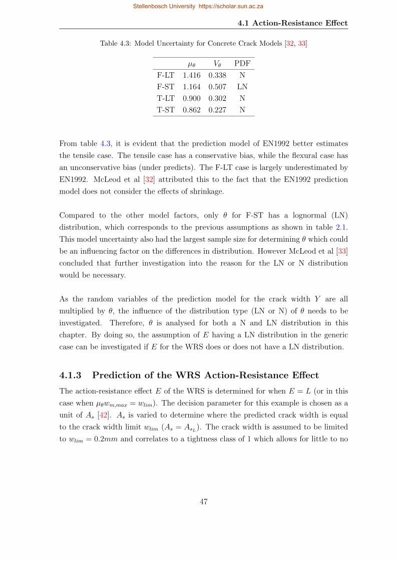
4.1 Action-Resistance Effect
Table 4.3: Model Uncertainty for Concrete Crack Models [32, 33]
µθ Vθ PDF
F-LT 1.416 0.338 N
F-ST 1.164 0.507 LN
T-LT 0.900 0.302 N
T-ST 0.862 0.227 N
From table 4.3, it is evident that the prediction model of EN1992 better estimates
the tensile case. The tensile case has a conservative bias, while the flexural case has
an unconservative bias (under predicts). The F-LT case is largely underestimated by
EN1992. McLeod et al [32] attributed this to the fact that the EN1992 prediction
model does not consider the effects of shrinkage.
Compared to the other model factors, only θ for F-ST has a lognormal (LN)
distribution, which corresponds to the previous assumptions as shown in table 2.1.
This model uncertainty also had the largest sample size for determining θ which could
be an influencing factor on the differences in distribution. However McLeod et al [33]
concluded that further investigation into the reason for the LN or N distribution
would be necessary.
As the random variables of the prediction model for the crack width Y are all
multiplied by θ, the influence of the distribution type (LN or N) of θ needs to be
investigated. Therefore, θ is analysed for both a N and LN distribution in this
chapter. By doing so, the assumption of E having a LN distribution in the generic
case can be investigated if E for the WRS does or does not have a LN distribution.
4.1.3 Prediction of the WRS Action-Resistance Effect
The action-resistance effect E of the WRS is determined for when E = L (or in this
case when µθwm,max = wlim). The decision parameter for this example is chosen as a
unit of As [42]. As is varied to determine where the predicted crack width is equal
to the crack width limit wlim (As = AsL). The crack width is assumed to be limited
to wlim = 0.2mm and correlates to a tightness class of 1 which allows for little to no
47
Stellenbosch University https://scholar.sun.ac.za

4.1 Action-Resistance Effect
leakage.
The mean-maximum crack width of two WRS (water retaining structures) is
calculated according to EN1992 for both flexural and tensile cracking. Short and
long term cracking are investigated to determine which one governs. The amount
of reinforcement AsL for the four scenarios is determined so that µE = wlim. The
two WRS have different thickness’s, bar diameters, and covers to investigate the
influences of these parameters on βt,SLS. The two water retaining structures are
named WRS 1 and WRS 2.
The sectional and material properties of the WRS are summarised in table 4.4. Both
WRS are designed to have a volume of V = 1500m3. The dimensions are defined
as: height H = 5m, diameter D = 20m, and thickness h = 500mm or 350mm for
WRS 1 and 2 respectively. The diameter of the structure has no influence on the
flexural design as the crack width is determined per meter strip (b = 1m). However
for tension, the diameter of the WRS is used to determine the hoop tension in the wall.
Table 4.4: WRS Section and Material Properties
Variable Symbol WRS1 WRS 2 Units
Diameter D 20.0 20.0 m
Height H 5.0 5.0 m
Width b 1.0 1.0 m
Wall Thickness h 500.0 350.0 mm
Cover c 40.0 30.0 mm
Diameter φ 20.0 25.0 mm
Concrete Tensile Strength fc,tm 2.6 2.6 MPa
Concrete Modulus Ec,ST 31.0 31.0 GPa
Elastic modulus of steel Es 200.0 200.0 GPa
Density of Water γw 10.0 10.0 kN/m2
Area of reinforcement AsL varies∗ mm2
* varies due to µθ to determine µE = wlim
The effect of the water is the main load on the structure. The density of the water
is γw = 10kN/m2 and is considered as a quasi permanent load. Concrete with a
48
Stellenbosch University https://scholar.sun.ac.za
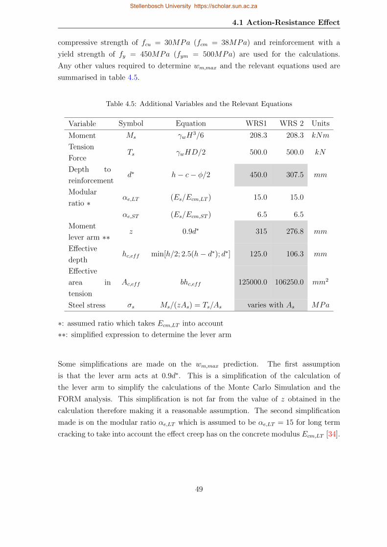
4.1 Action-Resistance Effect
compressive strength of fcu = 30MPa (fcm = 38MPa) and reinforcement with a
yield strength of fy = 450MPa (fym = 500MPa) are used for the calculations.
Any other values required to determine wm,max and the relevant equations used are
summarised in table 4.5.
Table 4.5: Additional Variables and the Relevant Equations
Variable Symbol Equation WRS1 WRS 2 Units
Moment Ms γwH3/6 208.3 208.3 kNm
Tension
ForceTs γwHD/2 500.0 500.0 kN
Depth to
reinforcementd∗ h− c− φ/2 450.0 307.5 mm
Modular
ratio ∗αe,LT (Es/Ecm,LT ) 15.0 15.0
αe,ST (Es/Ecm,ST ) 6.5 6.5
Moment
lever arm ∗∗z 0.9d∗ 315 276.8 mm
Effective
depthhc,eff min[h/2; 2.5(h− d∗); d∗] 125.0 106.3 mm
Effective
area in
tension
Ac,eff bhc,eff 125000.0 106250.0 mm2
Steel stress σs Ms/(zAs) = Ts/As varies with As MPa
∗: assumed ratio which takes Ecm,LT into account
∗∗: simplified expression to determine the lever arm
Some simplifications are made on the wm,max prediction. The first assumption
is that the lever arm acts at 0.9d∗. This is a simplification of the calculation of
the lever arm to simplify the calculations of the Monte Carlo Simulation and the
FORM analysis. This simplification is not far from the value of z obtained in the
calculation therefore making it a reasonable assumption. The second simplification
made is on the modular ratio αe,LT which is assumed to be αe,LT = 15 for long term
cracking to take into account the effect creep has on the concrete modulus Ecm,LT [34].
49
Stellenbosch University https://scholar.sun.ac.za

4.2 Generic βt,SLS for the WRS Obtained from the Generic Table
AsL for µE = wlim is determined for each cracking scenario, and the calculations are
shown in appendix B. AsL varies for the four scenarios based on the model factor
θ, the load type k2, and the load duration kt. LT cracking governs for both flexure
and tension. The results are shown in table 4.6 along with µθ and wm,max for each
scenario. F-LT cracking requires the most reinforcement to achieve the prescribed
limit for both WRS 1 and 2. This is mainly due to the high unconservative bias of
the model uncertainty.
It is observed from table 4.6 that for tension, there is no difference in AsL to obtain
the limit. The main reason for this is that the depth of the section h has a negligible
influence on the steel stress of the section.
Table 4.6: Amount of Reinforcement AsL for E = wlim
AsL (WRS 1) AsL (WRS 2) θ wm,max E
mm2 mm2 mm mm
F-LT 3184 4244 1.42 0.14 0.20
F-ST 2568 3615 1.16 0.17 0.20
T-LT 3026 3057 0.90 0.22 0.20
T-ST 2698 2796 0.86 0.23 0.20
As E is governed by both F-LT and T-LT, βt,SLS will be governed by either F-LT
or T-LT. Therefore, it is necessary to further investigate only these two scenarios in
determining βt,SLS for both WRS. From the crack width equations (equations 4.5
and 4.6), the random variables can be assigned statistical properties. From these
random variables the coefficient of variation for the crack width and the action
resistance effect can be determined.
4.2 Generic βt,SLS for the WRS Obtained from
the Generic Table
This section shows how to obtain the generic βt,SLS for the WRS from the generic
development of chapter 3. First the coefficient of variation of the WRS is computed
for both F-LT and T-LT. Next the cost ratio for the WRS is quantified. From these
50
Stellenbosch University https://scholar.sun.ac.za

4.2 Generic βt,SLS for the WRS Obtained from the Generic Table
specific values for the WRS, βt,SLS can be obtained.
4.2.1 Calculation of VE for the WRS
The coefficient of variation of the action-resistance effect VE is calculated to determine
βt,SLS from table 3.3. As E consists of random variables with their own statistical
parameters, VE needs to be calculated from these random variables. Two methods are
used to determine VE. First, Monte Carlo is used to accurately determine VEMCSand
also the distribution of E. Next an approximation of VEAPPis done and compared to
the results of the Monte Carlo simulation.
4.2.1.1 Monte Carlo Simulation
A brief overview of Monte Carlo Simulation is provided. The Monte Carlo simulation
is then performed on E of the two WRS to determine VEMCS.
The Monte Carlo simulation (MCS) technique is based on the random sampling of
variables [13]. The MCS is a simple random sampling method or statistical trial
method that makes realizations based on randomly generated sampling sets for
uncertain variables [39].
Choi et al [5] and El-Reedy [39] both set out the simple MCS procedure through the
following steps. These steps are simply shown in figure 4.2.
1. The first step is to select the distribution type(s) for the random variable(s).
Each random variable is described by three statistical parameters: mean,
standard deviation and distribution type. The input is shown in figure 4.2
by the distribution type, however, it the mean and standard deviation of that
random variable.
2. The next step is to generate a sampling set from the distribution(s) for the
chosen sample size. A sampling set is generated for the action-resistance effect
of the WRS. A large sample size is chosen based on the mathematical theory
that sample averages tend to stabilize as the sample increases [6].
51
Stellenbosch University https://scholar.sun.ac.za

4.2 Generic βt,SLS for the WRS Obtained from the Generic Table
3. The final step is to conduct simulations using the generated sampling set. The
generated sample set, or in this case wm,max, has a mean and standard deviation
while distribution type can be determined from the frequency distribution.
Figure 4.2: Monte Carlo Simulation [39]
The Monte Carlo Simulation (MCS) is performed using the trial version of the
@RISK [40] software which is an Excel add-in. From the MCS, the coefficient of
variation VEMCSand distribution of the action-resistance effect can be determined.
The random variables that the crack width comprises of and the model uncertainty
are the input variables for the MCS. The random variables and their statistical
properties for the MCS are shown in table 4.7. It is assumed that the statistical
properties (Vi and PDF) for WRS 1 and 2 are the same. The assumptions for
the random variables are made based on what is currently available in literature.
From table 4.7, the probability density function (PDF) of the variables is either
deterministic (det), normal (N), or lognormal (LN).
In table 4.7, the amount of reinforcement is defined as AsL . This is because AsLrequired such that µE = wlim is different for the two structures under consideration.
52
Stellenbosch University https://scholar.sun.ac.za

4.2 Generic βt,SLS for the WRS Obtained from the Generic Table
Table 4.7: Statistical Parameters of the WRS
Variable Units PDF µi Vi Ref
Moment Ms kNm N 208.0 0.05 [14, 18]
Tension Ts kN/m N 500.0 0.05 [14, 18]
Wall Height H m N 5.0 0.01 [18]
Wall Diameter D m N 20.0 0.01 [18]
Width b m det 1000.0 0.00 [14, 35]
Wall Thickness h mm LN 500.0/350.0 0.01
Cover c mm LN 40.0 /30.0 0.15 [35]
Diameter φ mm det 20.0/25.0 0.00 [14, 25, 30]
Elastic modulus
of steelEs GPa det 200.0 0.00 [14, 25, 35]
Concrete Tensile
Strengthfctm MPa LN 2.6 0.10 [35]
Strength Factors k1, k2, k3, kt det k 0.00 [14, 30]
Reinforcement
AreaAsL mm2 N AsL 0.02 [18, 27]
Model
UncertaintyF-LT θ N/LN 1.4 0.34 [32]
T-LT θ N/LN 0.9 0.30 [33]
For WRS 1, AsL = 3200mm2 and 3000mm2 for F-LT and T-LT respectively. Similarly
for WRS 2, AsL = 4300mm2 and 3000mm2 for F-LT and T-LT respectively.
From figure 4.2, the values in table 4.7 are entered as the inputs, @RISK is used as
the simulation model, and the outputs obtained from @RISK are further discussed
in this section.
The results of the output of the MCS using @RISK are summarised in table 4.8.
The coefficient of variation was determined for both wm,max and E. As the statistical
properties of WRS 1 and WRS 2 are assumed to be the same, both VEMCSand
Vwm,max for the two WRS are the same. The influence of Vθ on VEMCSis evident in
the results. Therefore the importance of choosing the correct model factor should
not be overlooked. The distribution (N or LN) of θ also has no influence on VEMCS
53
Stellenbosch University https://scholar.sun.ac.za
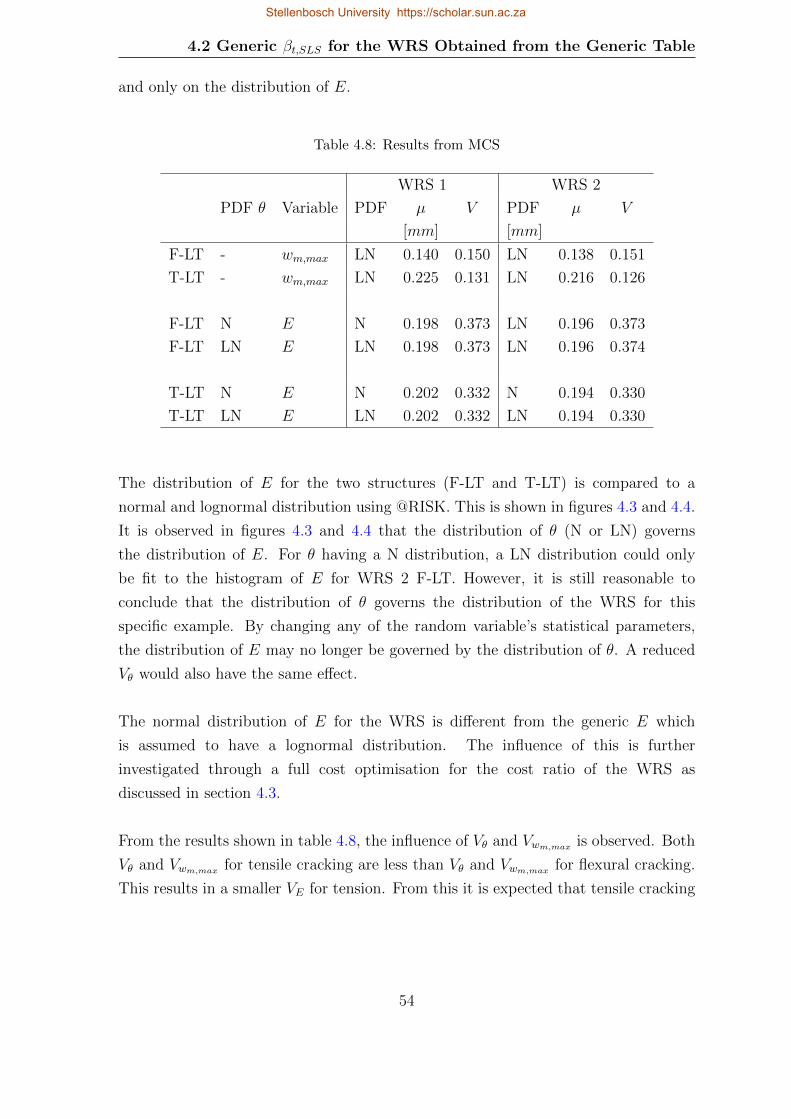
4.2 Generic βt,SLS for the WRS Obtained from the Generic Table
and only on the distribution of E.
Table 4.8: Results from MCS
WRS 1 WRS 2
PDF θ Variable PDF µ V PDF µ V
[mm] [mm]
F-LT - wm,max LN 0.140 0.150 LN 0.138 0.151
T-LT - wm,max LN 0.225 0.131 LN 0.216 0.126
F-LT N E N 0.198 0.373 LN 0.196 0.373
F-LT LN E LN 0.198 0.373 LN 0.196 0.374
T-LT N E N 0.202 0.332 N 0.194 0.330
T-LT LN E LN 0.202 0.332 LN 0.194 0.330
The distribution of E for the two structures (F-LT and T-LT) is compared to a
normal and lognormal distribution using @RISK. This is shown in figures 4.3 and 4.4.
It is observed in figures 4.3 and 4.4 that the distribution of θ (N or LN) governs
the distribution of E. For θ having a N distribution, a LN distribution could only
be fit to the histogram of E for WRS 2 F-LT. However, it is still reasonable to
conclude that the distribution of θ governs the distribution of the WRS for this
specific example. By changing any of the random variable’s statistical parameters,
the distribution of E may no longer be governed by the distribution of θ. A reduced
Vθ would also have the same effect.
The normal distribution of E for the WRS is different from the generic E which
is assumed to have a lognormal distribution. The influence of this is further
investigated through a full cost optimisation for the cost ratio of the WRS as
discussed in section 4.3.
From the results shown in table 4.8, the influence of Vθ and Vwm,max is observed. Both
Vθ and Vwm,max for tensile cracking are less than Vθ and Vwm,max for flexural cracking.
This results in a smaller VE for tension. From this it is expected that tensile cracking
54
Stellenbosch University https://scholar.sun.ac.za
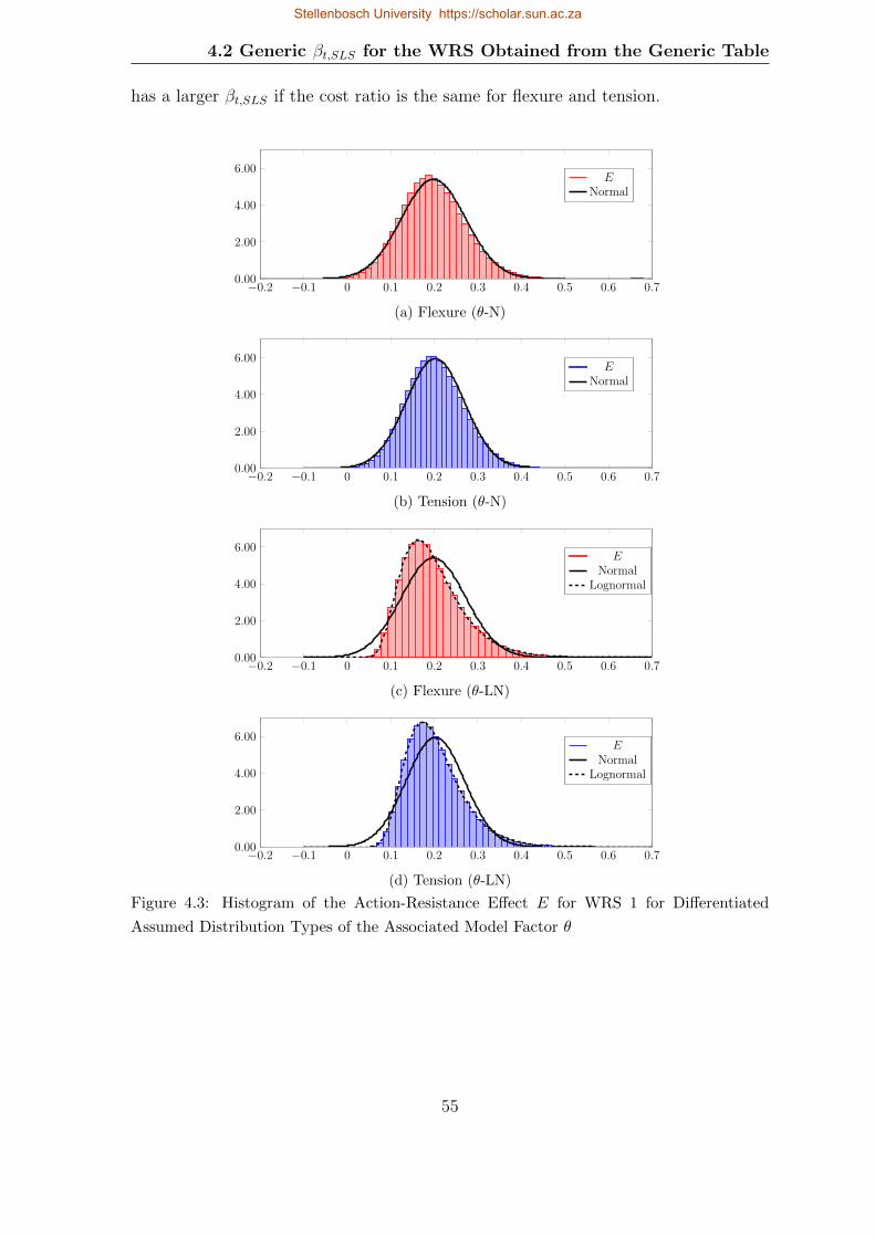
4.2 Generic βt,SLS for the WRS Obtained from the Generic Table
has a larger βt,SLS if the cost ratio is the same for flexure and tension.
−0.2 −0.1 0 0.1 0.2 0.3 0.4 0.5 0.6 0.70.00
2.00
4.00
6.00E
Normal
(a) Flexure (θ-N)
−0.2 −0.1 0 0.1 0.2 0.3 0.4 0.5 0.6 0.70.00
2.00
4.00
6.00E
Normal
(b) Tension (θ-N)
−0.2 −0.1 0 0.1 0.2 0.3 0.4 0.5 0.6 0.70.00
2.00
4.00
6.00E
NormalLognormal
(c) Flexure (θ-LN)
−0.2 −0.1 0 0.1 0.2 0.3 0.4 0.5 0.6 0.70.00
2.00
4.00
6.00E
NormalLognormal
(d) Tension (θ-LN)
Figure 4.3: Histogram of the Action-Resistance Effect E for WRS 1 for Differentiated
Assumed Distribution Types of the Associated Model Factor θ
55
Stellenbosch University https://scholar.sun.ac.za

4.2 Generic βt,SLS for the WRS Obtained from the Generic Table
−0.2 −0.1 0 0.1 0.2 0.3 0.4 0.5 0.6 0.70.00
2.00
4.00
6.00E
NormalLognormal
(a) Flexure (θ-N)
−0.2 −0.1 0 0.1 0.2 0.3 0.4 0.5 0.6 0.70.00
2.00
4.00
6.00E
Normal
(b) Tension (θ-N)
−0.2 −0.1 0 0.1 0.2 0.3 0.4 0.5 0.6 0.70.00
2.00
4.00
6.00E
NormalLognormal
(c) Flexure (θ-LN)
−0.2 −0.1 0 0.1 0.2 0.3 0.4 0.5 0.6 0.70.00
2.00
4.00
6.00E
NormalLognormal
(d) Tension (θ-LN)
Figure 4.4: Histogram of the Action-Resistance Effect E for WRS 2 for Differentiated
Assumed Distribution Types of the Associated Model Factor θ
56
Stellenbosch University https://scholar.sun.ac.za

4.2 Generic βt,SLS for the WRS Obtained from the Generic Table
4.2.1.2 Approximation of VE
It is not always possible to determine VE through MCS or any other sampling method.
If a quick estimate of VE is required, a complete MCS of a sufficient sample size is
time consuming. It is, therefore, necessary to consider an approach which quickly
approximates VE. A simplified method of determining VEAPPbased on the coefficient
of variation of the random variables Vi is conducted to compare these results to the
sampling analysis. For assumed normally distributed uncorrelated variables VEAPPis
determined through equation 4.7 [13, 36].
VEAPP=
√∑V 2i (4.7)
with VEAPPCoefficient of variation of the action-resistance effect.
Vi Coefficient of variation of the random variable i.
For the WRS, the 5 random variables identified are area of reinforcement, cover,
loading, concrete tensile strength and model uncertainty. Vi of the random variables
is obtained from table 4.7. VEAPPis the approximated for both flexure and tension.
The results for the approximation are shown in table 4.9 along with the results from
the MCS.
Table 4.9: Comparative Table of VE for the WRS
MCS APP
VEMCSVEAPP
F-LT 0.373 0.387
T-LT 0.332 0.356APP = approximation
(equation 4.7)
As seen in table 4.9, the approximated VEAPPis reasonably close to VEMCS
(∆VE ≈ 0.025). It is therefore a reasonable method for determining VE. Although
this method is quicker and yields similar results there is one major drawback to
using the simplified approach. The distribution of E cannot be determined for the
simplified calculation of VEAPP. However, if the assumption in the generic case of a
LN distribution holds for a non-lognormally distributed E, it may be reasonable to
57
Stellenbosch University https://scholar.sun.ac.za

4.2 Generic βt,SLS for the WRS Obtained from the Generic Table
conclude that this method is sufficient.
4.2.2 Calculation of the Costs
To obtain βt,SLS from table 3.3, the specific cost ratios Cf/C1 also need to be
quantified. This is done by determining the specific costs of providing safety C1 and
the specific failure costs Cf . The costs in this section are a simple representation of
some of the cost considerations when determining Cf/C1. The assumptions made
for these costs are stated in the respective subsections (section 4.2.2.1 and 4.2.2.2).
As a consistent unit of measurement is necessary, the costs for the two WRS are
calculated as Rand per meter squared (R/m2).
4.2.2.1 Costs of Providing Reinforcement C1
For the generic structure, the cost of providing safety is equal to the cost of one unit
of d. Since d = 1 implies that E = L for the generic structure (equation 3.9), the
cost of providing reinforcement C1 for the WRS must correlate to µE = wlim. For
the WRS, the decision parameter is the amount of reinforcement As. Therefore C1
is the cost of providing AsL such that µE = wlim. AsL is the area of reinforcement
required such that µE = wlim. It is assumed that all other construction costs C0 are
independent of AsL .
To determine C1 for the WRS, the cost per reinforcement bar is determined. The
cost to provide one bar of reinforcement is quoted as R10.20/kg [22]. The weight of
one bar (kg/m) is determined using equation 4.8. One Y20 (WRS 1) and Y25 (WRS
2) weigh ws = 2.47kg/m and 3.85kg/m respectively. C1 is then determined using
equation 4.9 as the cost per bar (R/kg) times the weight of the bar (kg/m) times the
number of bars per meter AsL/As1 (/m). The cost C1 for the two WRS is summarised
in table 4.10.
58
Stellenbosch University https://scholar.sun.ac.za

4.2 Generic βt,SLS for the WRS Obtained from the Generic Table
ws = ρφ2π
4(4.8)
C1 =AsLAs1× ws × 10.20 (4.9)
with ρ Density of steel ρ = 7850kg/m3
φ Bar diameter
AsL Area of reinforcement which results in E = wlim
As1 Area of reinforcement of one bar
Table 4.10: Cost of Providing Safety C1 for the WRS
AsL C1
mm2 R/m2
WRS 1 Y20 314 25.19
F-LT 3200 256.62
T-LT 3000 240.58
WRS 2 Y25 491 39.30
F-LT 4300 344.30
T-LT 3000 240.21
4.2.2.2 Failure Costs Cf
Quantifying the failure costs is considered to be the most difficult step in terms
of cost optimisation as both direct and indirect failure consequences need to be
considered [47]. For this example, the failure costs Cf are simplified to account only
for the failure costs associated with providing water tight lining for an already cracked
concrete section. Some of the other failure costs which may occur for a similar WRS
are indicated below:
• Labour costs required to place the lining.
• Costs for structural repairs of the concrete.
59
Stellenbosch University https://scholar.sun.ac.za

4.2 Generic βt,SLS for the WRS Obtained from the Generic Table
• Replacement costs of the reinforcement.
• Costs due to indirect consequences of failure.
• Costs related to emptying and filling the WRS during crack repair.
• Inspection costs to assess the extent of repairs required.
The failure costs are assumed to be Cf = R1500/m2. This is the cost to provide
water tight lining per square meter of the WRS. This seems reasonable from a
practical perspective.
4.2.2.3 Cost Ratio Cf/C1
From the quantified costs, C1 and Cf , the cost ratio can be calculated for flexural
and tensile cracking. The cost ratios are calculated using the generic framework
(Cf/C1). The cost ratios for both WRS are shown in table 4.11. From a practical
perspective, these cost ratios seem reasonable.
Table 4.11: Cost Ratio Cf/C1 for the WRS
C1 Cf Cf/C1
[R/m2] [R/m2]
WRS 1 F-LT 256.62 1500.00 5.9
WRS 1 T-LT 240.58 1500.00 6.2
WRS 2 F-LT 344.30 1500.00 4.5
WRS 2 T-LT 240.21 1500.00 6.2
The first observation, made from table 4.11, is that the cost ratios for T-LT for WRS
1 and WRS 2 are the same. This means that βt,SLS is the same for both structures.
On the other hand for F-LT, the cost ratio for WRS 1 is significantly higher than the
cost ratio for WRS 2. This is because the cost of providing reinforcement for WRS 1
is cheaper (smaller bar diameter) than WRS 2. The second observation made from
these results is that flexural cracking has a lower cost ratio than tensile cracking.
60
Stellenbosch University https://scholar.sun.ac.za

4.3 Specific βt,SLS for the WRS Determined from Cost Optimisation
This is because flexural cracking has a larger AsL than tensile cracking.
4.2.3 βtSLS for the WRS
As VE and Cf/C1 have been quantified, βt,SLS for the two WRS is obtained from
table 3.3. In this paper the statistical parameters for the two WRS did not vary,
resulting in the same VE for both structures. The cost ratios were also quantified
to be different for F-LT but the same for T-LT. Table 4.12 summarises the results
of the previous sections. From table 3.3 the target values βt,SLS can be determined.
The results from table 3.3 are also shown in table 4.12.
Table 4.12: βt,SLS for the WRS from the Generic Development
WRS VE Cf/C1 βt,SLS
F-LT 1 0.373 5.9 1.58
2 0.373 4.5 1.48
T-LT 1 0.332 6.2 1.68
2 0.332 6.2 1.68
4.3 Specific βt,SLS for the WRS Determined from
Cost Optimisation
The assumption made in the generic development of chapter 3 that E has a LN
distribution does not hold for the WRS. E for the crack width prediction of the WRS
has a N distribution as a result of the N distribution of the model uncertainty. To
check if the generic βt,SLS values still hold for the WRS with a normal distribution of
E a full reliability analysis and cost optimisation is done. The results from the cost
optimisation are then compared to the results obtained from table 3.3.
4.3.1 FORM Analysis
A FORM analysis in Risk Tools (RT) [41] on the limit state equation is performed
to determine T (As) of the WRS. E is replaced in the limit state equation with E =
θwm,max. As the crack width is calculated from the random variables of the input,
the crack width equation is inserted into E rather than the predicted mean-maximum
61
Stellenbosch University https://scholar.sun.ac.za

4.3 Specific βt,SLS for the WRS Determined from Cost Optimisation
crack width. The input limit state equations are shown in equations 4.10 and 4.11
for flexure and tension respectively. The input variables and their assumed statistical
parameters remain the same as for the Monte Carlo analysis and are shown in table 4.7.
g(1, wm,RT (F )) = 0.2− θ[3.4c+ 0.425k1k2(φhcb
As)]
×[Ms
zAsEs− ktfcthc
As
1 + αeAs/(hcb)
Es] (4.10)
g(1, wm,RT (T )) = 0.2− θ[3.4c+ 0.425k1k2(φhcb
As)]
×[TsAsEs
− ktfcthcAs
1 + αeAs/(hcb)
Es] (4.11)
For this example, As (the decision parameter) varies in increments of ∆As = 100mm2
for the four different scenarios. For WRS 1 flexure and tension, the range
As = [2900 − 6000]mm2 is considered. For WRS 2 flexure and tension, the ranges
As = [4000− 7500]mm2 and As = [3000− 5500]mm2 are considered. The ranges were
chosen based on the range of the generic case such that d = 0.2/E ≈ 3.
3000 3500 4000 4500 5000 5500 6000 6500 7000 75000.05
0.10
0.15
0.20
0.25
As
EwLIMWRS 1F-LTT-LTWRS 2F-LTT-LT
Figure 4.5: E for Varying As
E is shown in figure 4.5, the calculations are shown in appendix B. As was identified
in section 4.1.3, E has the same amount of reinforcement for both WRS in tension.
This is because changing the thickness of the section has no influence on the steel
62
Stellenbosch University https://scholar.sun.ac.za

4.3 Specific βt,SLS for the WRS Determined from Cost Optimisation
stress in tension. The thickness of the section does, however, have a significant
role on the flexural prediction model resulting in more reinforcement required for a
thinner section. This influence on E is further observed with the results from the
FORM analysis.
Equations 4.10 and 4.11 are entered into RT and a FORM analysis is performed.
θ and consequently E are considered with both a LN and N distribution. The
β(As) values obtained are shown in figure 4.6 as the β(As) versus the amount of
reinforcement As. The influence of the distribution choice is not negligible towards
the tail end of E. The influence on the assumption of the distribution is further
observed with the cost optimisation of the WRS.
As identified, h has a negligible influence on E for the tensile load case of the WRS.
As expected there is also a negligible difference for β(As) for tensile crack width
predictions.
3000 3500 4000 4500 5000 5500 6000 6500 7000 75000.0
1.0
2.0
3.0
4.0
As
β(As)
WRS1F-LT (N)T-LT (N)F-LT (LN)T-LT (LN)WRS2F-LT (N)T-LT (N)F-LT (LN)T-LT (LN)
Figure 4.6: β(As) vs As of WRS
63
Stellenbosch University https://scholar.sun.ac.za
4.3 Specific βt,SLS for the WRS Determined from Cost Optimisation
4.3.2 βt,SLS from Cost Optimisation
For the WRS, As is chosen to be the decision parameter. To perform a cost
optimisation the cost of providing safety C1 depends on how many bars are required
to provide sufficient reinforcement per meter. C1 and Cf are determined using
equations 4.13 and 4.14 respectively. Cost optimisation is then performed using
equation 4.12 as described in section 3.1.
Ctot = C1As + Cfpf (As) (4.12)
Where:
C1 =1
As1× ws × 10.20 (4.13)
Cf = R1500/m2 (4.14)
with C1 Cost of providing reinforcement per square meter
per square millimeter increase in As for the WRS
Cf Failure costs for the WRS
As Amount of reinforcement - decision parameter for the WRS
pf (As) Probability of failure as a function of As
ws Weight of one bar of reinforcement
The results for the economic optimisation are shown in table 4.13. The difference
between the βt,SLS for LN and N is negligible. The two WRS resulted in the similar
βt,SLS values. This is expected as the statistical parameters for the two structures
remained the same and the costs resulted in similar cost ratios for the two cases.
It was predicted that the results from the cost optimisation of the WRS would match
the results of the βt,SLS values determined from table 3.3. However, this is not the
case for the two structures. For the comparison of the two results, a difference of
∆βt,SLS ≈ 0.6 and ∆βt,SLS ≈ 0.4 is observed for a N and LN distribution of E
respectively. From this difference in the results, it is evident that an assumption
or generalisation made for the generic structure that does not hold for the WRS.
The assumption that E has a LN distribution has no significant influence on the
discrepancy of the results. An investigation into what caused this discrepancy is
done in chapter 6.
64
Stellenbosch University https://scholar.sun.ac.za

4.3 Specific βt,SLS for the WRS Determined from Cost Optimisation
Table 4.13: βt,SLS for the WRS
From Table 3.3 Cost Optimisation
WRS Section 4.2.3 N LN
F-LT 1 1.6 2.2 1.9
2 1.5 2.1 1.9
T-LT 1 1.7 2.2 2.1
2 1.7 2.3 2.2
4.3.3 Concluding Remarks
This chapter determined the βt,SLS for two WRS. First, E of the WRS is determined,
by using the Eurocode’s crack width prediction model wm,max multiplied by the
model uncertainty θ based on the same prediction model. The two WRS differed in
thickness, cover and bar diameter. The prediction of the crack width is considered
for both flexural and tensile cracking as well as long and short term loading. The
amount of reinforcement AsL is determined so that E = L (where L = wlim = 0.2).
For both flexural and tensile cracking, AsL is governed by long term loading for the
two structures investigated.
Once E is determined the coefficient of variation VE could be determined. VE is
determined by both Monte Carlo Simulation and an approximation that assumes
normally distributed uncorrelated variables. The approximation is identified as
a suitable method for determining VE as the results obtained are similar to the
MCS. From the MSC, the distribution of E is determined to be N as a result of
the N distribution of θ. The generic development of chapter 3 assumed E to be
lognormally distributed, θ and consequently E are considered to have both N and LN
distributions. VE is calculated as 0.373 and 0.332 for flexure and tension respectively.
The two WRS had the same distribution for E.
The next step was to quantify the costs for the specific structure. The cost of
providing reinforcement C1 per square meter was calculated for AsL (resulting in
µE = wlim) and the failure costs were assumed to be Cf = R1500/m2. For F-LT, the
cost ratios were quantified as Cf/C1 = 5.9 and 4.5 for WRS 1 and 2 respectively, and
65
Stellenbosch University https://scholar.sun.ac.za
4.3 Specific βt,SLS for the WRS Determined from Cost Optimisation
for T-LT, Cf/C1 = 6.2 for both WRS.
βt,SLS was then read from table 3.3 and is summarised in table 4.13. To determine
if these target values from the generic development hold for the specific application,
both normal and lognormal distributions of E, a cost optimisation is done. These
results are summarised in table 4.13. A discrepancy in the results obtained from
the generic development and the specific structure occurred. The reason for this
discrepancy is further investigated in the subsequent chapters.
66
Stellenbosch University https://scholar.sun.ac.za
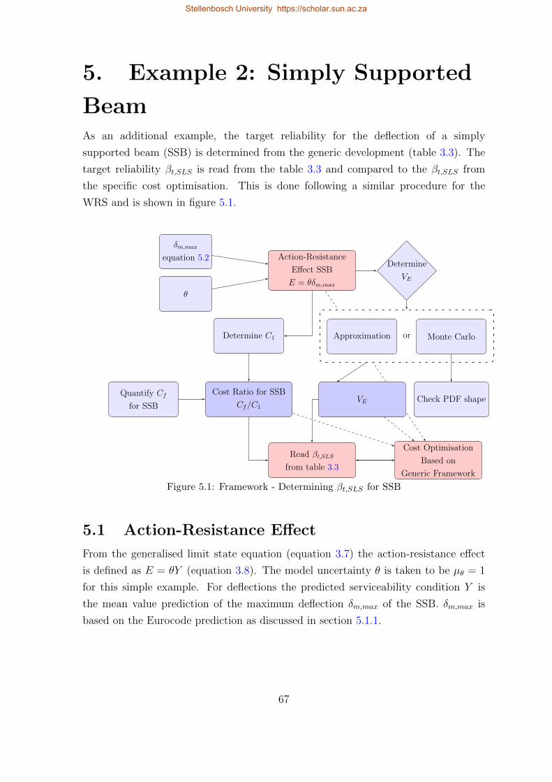
5. Example 2: Simply Supported
BeamAs an additional example, the target reliability for the deflection of a simply
supported beam (SSB) is determined from the generic development (table 3.3). The
target reliability βt,SLS is read from the table 3.3 and compared to the βt,SLS from
the specific cost optimisation. This is done following a similar procedure for the
WRS and is shown in figure 5.1.
Action-Resistance
Effect SSB
E = θδm,max
Determine C1
Cost Ratio for SSB
Cf/C1
Quantify Cf
for SSB
Determine
VE
orApproximation Monte Carlo
Check PDF shapeVE
Read βt,SLS
from table 3.3
Cost Optimisation
Based on
Generic Framework
δm,max
equation 5.2
θ
Figure 5.1: Framework - Determining βt,SLS for SSB
5.1 Action-Resistance Effect
From the generalised limit state equation (equation 3.7) the action-resistance effect
is defined as E = θY (equation 3.8). The model uncertainty θ is taken to be µθ = 1
for this simple example. For deflections the predicted serviceability condition Y is
the mean value prediction of the maximum deflection δm,max of the SSB. δm,max is
based on the Eurocode prediction as discussed in section 5.1.1.
67
Stellenbosch University https://scholar.sun.ac.za

5.1 Action-Resistance Effect
5.1.1 Deflection Equation
δm,max is calculated, following the provisions of section 7.4.3 in EN1992-1-1 [8].
Honfi’s [21] interpretation of equation 5.1 is used as shown in equation 5.2. This is
based on the well-known maximum deflection equation for a simply supported beam
(5
384
qL4
EI).
α = ξαII + (1− ξ)αI (5.1)
δm,max = ξ5
384
qL4
Ec,effI2+ (1− ξ) 5
384
qL4
Ec,effI1(5.2)
with α Deformation parameter
αI Deformation - uncracked
αII Deformation - fully cracked
ξ Distribution coefficient (allowing for tension stiffening)
q Distributed Load
L Span of the beam
Ec,eff Long term effective concrete modulus taking shrinkage into account
I1 Moment of inertia - uncracked
I2 Moment of inertia - fully cracked
The distribution coefficient ξ which allows for tension stiffening is calculated using
equation 5.3. As the beam is subjected to a flexural load, ξ is written in terms of the
SLS moment Ms and cracking moment Mcr. The distributed load q is a combination of
the permanent and imposed load (G and Q) over the span of the beam. The long term
effective concrete modulus is calculated using equation 5.4. The moment of inertia
for the uncracked and cracked section is shown in equations 5.5 and 5.6 respectively.
Equation 5.6 comes from course notes [51]. For this example it is assumed that the
load which induces deflections is a sustained load, therefore, βξ = 0.5. The moments
Mcr and Ms are calculated using equations 5.7 and 5.8 respectively.
68
Stellenbosch University https://scholar.sun.ac.za
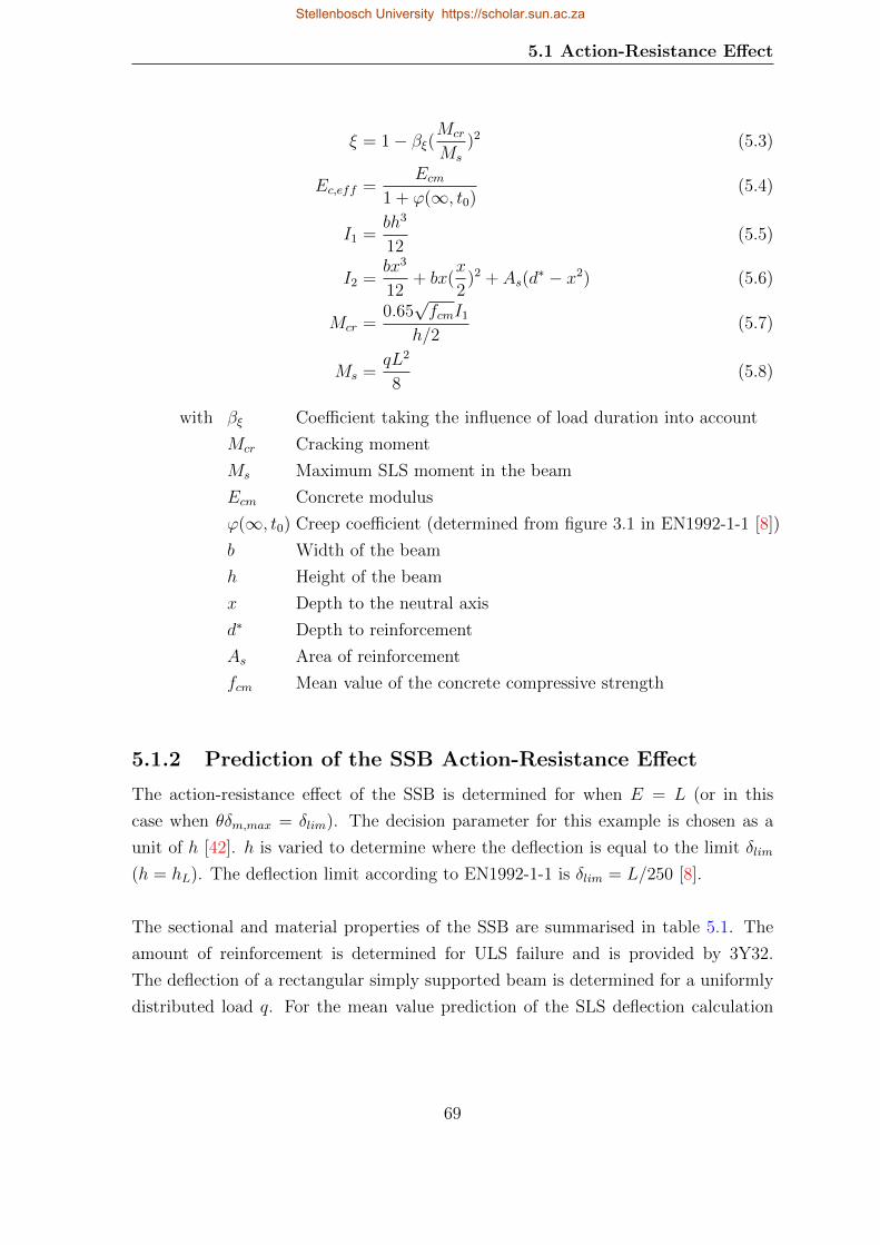
5.1 Action-Resistance Effect
ξ = 1− βξ(Mcr
Ms
)2 (5.3)
Ec,eff =Ecm
1 + ϕ(∞, t0)(5.4)
I1 =bh3
12(5.5)
I2 =bx3
12+ bx(
x
2)2 + As(d
∗ − x2) (5.6)
Mcr =0.65√fcmI1
h/2(5.7)
Ms =qL2
8(5.8)
with βξ Coefficient taking the influence of load duration into account
Mcr Cracking moment
Ms Maximum SLS moment in the beam
Ecm Concrete modulus
ϕ(∞, t0) Creep coefficient (determined from figure 3.1 in EN1992-1-1 [8])
b Width of the beam
h Height of the beam
x Depth to the neutral axis
d∗ Depth to reinforcement
As Area of reinforcement
fcm Mean value of the concrete compressive strength
5.1.2 Prediction of the SSB Action-Resistance Effect
The action-resistance effect of the SSB is determined for when E = L (or in this
case when θδm,max = δlim). The decision parameter for this example is chosen as a
unit of h [42]. h is varied to determine where the deflection is equal to the limit δlim
(h = hL). The deflection limit according to EN1992-1-1 is δlim = L/250 [8].
The sectional and material properties of the SSB are summarised in table 5.1. The
amount of reinforcement is determined for ULS failure and is provided by 3Y32.
The deflection of a rectangular simply supported beam is determined for a uniformly
distributed load q. For the mean value prediction of the SLS deflection calculation
69
Stellenbosch University https://scholar.sun.ac.za

5.1 Action-Resistance Effect
the mean values of the permanent and variable loads are taken and not the design
values. The mean value of the concrete compressive strength fcm is taken from table
3.1 in EN1992-1-1 [8] and corresponds to fcu = 30MPa.
Table 5.1: Simply Supported Beam - Assumed Variables
Variable Symbol Value Units
Length L 7.5 m
Width b 350.0 mm
Thickness hL 485.0 mm
Cover c 25.0 mm
Concrete Compressive Strength fcm 38.0 MPa
Concrete Modulus Ec 31.0 GPa
Steel Yield Stress fy 450.0 MPa
Steel Modulus Es 200.0 GPa
Diameter φ 32.0 mm
Area of reinforcement As 2412.7 mm2
Permanent Load G 8.0 kN/m
Imposed/Variable Load Q 5.0 kN/m
Some simplifications are made to simplify the limit state equation for the Monte
Carlo Simulation and FORM analysis. First the long term effective concrete modulus
Ec,eff (equation 5.4) is assumed to be 13MPa. This assumption comes from the
assumption in chapter 4 that the modular ratio is αE = 15. The second assumption is
to determine the fully cracked moment of inertia I2 as a percentage f of the uncracked
moment of inertia I1. This is shown in equation 5.9. For this example f = 37% and
is determined as the average percentage I2 is of I1 based on the investigated range of
h = [470 − 620]mm. The calculations showing the difference in δm,max based on this
assumption is shown in appendix C. As seen in figure 5.2 this simplification does not
have a significant effect on δm,max.
I2 = fbh3
12(5.9)
Figure 5.2 shows the calculated µE (for µθ = 1.0) for varying h. The depth of the
section is studied for the range h = [470− 620]mm in increments of ∆h = 5mm. The
70
Stellenbosch University https://scholar.sun.ac.za

5.2 Generic βt,SLS for the SSB Obtained from the Generic Table
deflection requirement (δlim = 30) is satisfied when hL = 485mm. Both the extensive
calculation of δm,max using equation 5.6 to determine the cracked moment of inertia
and the simplified calculation of δm,max using equation 5.9 to determine the cracked
moment of inertia are shown in figure 5.2.
480 500 520 540 560 580 600 62010
20
30
h [mm]
µE [mm] δlimI2
simplifiedextensive
Figure 5.2: Deflection for Varying h
5.2 Generic βt,SLS for the SSB Obtained from the
Generic Table
This section shows how to obtain the generic βt,SLS for the SSB from table 3.3. First
the coefficient of variation of the SSB is computed. Next the cost ratio for the SSB
is quantified. From these specific values for the SSB, βt,SLS can be obtained.
5.2.1 Calculation of VE for the SSB
The coefficient of variation of the action-resistance effect VE is necessary to obtain
βt,SLS from table 3.3. Two methods are used to determine VE. First, Monte Carlo
Simulation (MCS) is used to accurately determine VEMCSand the distribution of E.
An approximation of VEAPPis done and compared to the results of the MCS. These
two methods are described in section 4.2.1
The random variables of the deflection prediction model and the model uncertainty
corresponding to this deflection prediction model are the input variables for the MCS.
These random variables and their statistical properties are shown in table 5.2. The
assumptions for the random variables are made based on what is currently available
71
Stellenbosch University https://scholar.sun.ac.za

5.2 Generic βt,SLS for the SSB Obtained from the Generic Table
in literature. From table 5.2, the probability density function (PDF) of the variables
is either deterministic (det), Normal (N), or lognormal (LN).
Table 5.2: Statistical Parameters of the SSB
Variable Units PDF Mean V Ref
Dead Load DL kN/m N 8 0.05 [18]
Live Load LL kN/m LN 5 0.20 [18]
Length L m det 15 0.00 [18, 26]
Width b m det 350 0.00 [18, 26]
Beam Height hL mm LN 485 0.02 [18, 26]
Concrete Modulus Ec,eff GPa LN 13 0.04 [21]
Concrete Compressive Strength fcm MPa LN 38 0.17 [21]
Model Uncertainty θ LN 1 0.10 [21]
The results from the MCS using @RISK are summarised with the results from the
approximation in table 5.3. The distribution of E for SSB was fit using @RISK to
a normal and lognormal distribution. This is shown in figure 5.3. It is observed in
figure 5.3 that E has a LN distribution.
15 20 25 30 35 40 45 500.00
0.02
0.04
0.06
0.08
0.10
ENormal
Lognormal
Figure 5.3: Histogram of the Action-Resistance Effect for the SSB
For the SSB, VEAPPis almost double VEMCS
. VEMCSis determined by sampling
random variables whereas VEAPPassumes that the variables are uncorrelated and
normally distributed, therefore, VEMCSis correct for the SSB. The difference in VE for
the two methods is due to two reasons. The first is that the approximation is made
on the assumption that normally distributed uncorrelated variables are used. This
72
Stellenbosch University https://scholar.sun.ac.za

5.2 Generic βt,SLS for the SSB Obtained from the Generic Table
Table 5.3: VE for the SSB
PDF MCS APP
VEMCSVEAPP
Deflections LN 0.164 0.287
is not true for deflections as most of the random variables have a LN distribution.
The second reason is from the complexity of the deflection equation. For the WRS,
Vθ was so large that it governed VE. However, for the SSB, Vθ is relatively small
compared to the other random variables such that it had a negligible influence on VE.
Using the higher VEAPPresults in a significantly lower βt,SLS than the βt,SLS
obtained from the lower VEMCS. The approximation results in an unconservative
recommendation for the target reliability of the SSB. It is, therefore, recommended
that a full MCS or sampling analysis be performed to determine VE.
5.2.2 Calculation of the Cost Ratio
To obtain βt,SLS from table 3.3, the specific cost ratios Cf/C1 also need to be
quantified. This is done by determining the specific costs of providing safety C1 and
the specific failure costs Cf . The costs in this section are a simple representation of
some of the cost considerations when determining Cf/C1. As a consistent unit of
measurement is necessary, the costs for the SSB are calculated in Rands (R).
For the generic structure, the cost of providing safety is equal to the cost of one unit
of d. Since d = 1 implies that E = L for the generic structure (equation 3.9), the
cost of providing concrete C1 for the SSB must correlate to µE = δlim. For the SSB,
the decision parameter is the depth of the section h. Therefore C1 is the cost of
providing hL such that µE = δlim. hL is the depth of the beam such that µE = δlim.
It is assumed that all other construction costs C0 are independent of hL.
To determine C1 for the SSB, the cost to provide concrete. The cost of concrete per
cubic meter is R2500/m3 [29]. C1 is then determined using equation 5.10 as the cost
per per cubic meter(R/m3) times the width (m) times the height (m) times length
73
Stellenbosch University https://scholar.sun.ac.za

5.2 Generic βt,SLS for the SSB Obtained from the Generic Table
(L). The cost C1 is calculated as C1 = R3182.85.
C1 = bhLL×R2500/m3 (5.10)
with b Width (b = 0.350m)
hL Height so that µE = δlim (h = 0.485m)
L Length (L = 7.5m)
For the SSB, the failure costs Cf are simply assumed to be equal to R6000 and is the
cost associated with strengthening the beam. From the quantified costs, C1 and Cf ,
the cost ratio can be for the SSB. The cost ratios are calculated Cf/C1 = 1.9. This
cost ratio seems reasonable from a practical perspective.
5.2.3 βt,SLS for the SSB
As VE and Cf/C1 have been quantified, βt,SLS for the SSB is read from table 3.3. VE
is taken as the result of the MCS and the approximation (APP). This is to show how
an error in calculating VE influences the resulting βt,SLS.
Table 5.4: βt,SLS for the SSB from the Generic Development
VE Cf/C1 βt,SLS
MCS 0.157 1.9 1.61
APP 0.287 1.9 1.16
Table 5.4 highlights where βt,SLS for the SSB is read from the table. The error in the
VE from the approximation is apparent. For the VE from MCS, βt,SLS = 1.6 while for
the approximation βt,SLS = 1.2. This results in ∆βt,SLS = 0.4 which is a considerably
large difference in the recommended target reliability for the SSB.
74
Stellenbosch University https://scholar.sun.ac.za
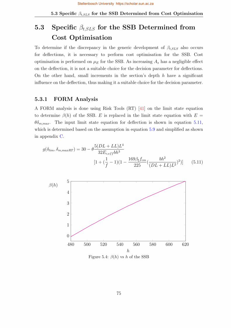
5.3 Specific βt,SLS for the SSB Determined from Cost Optimisation
5.3 Specific βt,SLS for the SSB Determined from
Cost Optimisation
To determine if the discrepancy in the generic development of βt,SLS also occurs
for deflections, it is necessary to perform cost optimisation for the SSB. Cost
optimisation is performed on µE for the SSB. As increasing As has a negligible effect
on the deflection, it is not a suitable choice for the decision parameter for deflections.
On the other hand, small increments in the section’s depth h have a significant
influence on the deflection, thus making it a suitable choice for the decision parameter.
5.3.1 FORM Analysis
A FORM analysis is done using Risk Tools (RT) [41] on the limit state equation
to determine β(h) of the SSB. E is replaced in the limit state equation with E =
θδm,max. The input limit state equation for deflection is shown in equation 5.11,
which is determined based on the assumption in equation 5.9 and simplified as shown
in appendix C.
g(δlim, δm,maxRT ) = 30− θ5(DL+ LL)L4
32Ec,effbh3
[1 + (1
f− 1)(1− 169βξfcm
225(
bh2
(DL+ LL)L2)2)] (5.11)
480 500 520 540 560 580 600 620
0
1
2
3
4
5
h
β(h)
Figure 5.4: β(h) vs h of the SSB
75
Stellenbosch University https://scholar.sun.ac.za
5.3 Specific βt,SLS for the SSB Determined from Cost Optimisation
The input variables and their assumed statistical parameters are the same as for the
MCS as shown in table 5.2. For this example h (the decision parameter) is studied
for the range h = [470 − 620]mm in increments of ∆h = 5mm. The β(h) values
obtained from the FORM analysis are shown in figure 5.4 as the β(h) versus the
depth of the section h.
5.3.2 βt,SLS from Cost Optimisation
The costs in this section are a simple representation of some of the cost considerations
when determining Cf/C1. As a consistent unit of measurement is necessary, the costs
for the SSB are calculated in Rands (R).
For the SSB, h is chosen to be the decision parameter. The cost of providing concrete
C1 depends on how much concrete is required per meter of h. The cost of concrete
per cubic meter is R2500/m3 [29]. C1 is then calculated using equation 5.13. The
failure costs Cf are assumed to be the cost of strengthening the beam and are equal
to R6000/m (per meter of beam).
Once the costs have been quantified cost optimisation is then performed using
equation 5.12 as described in section 3.1.
Ctot = C1h+ Cfpf (h) (5.12)
Where:
C1 = bL×R2500/m3 = R6562.50/m (5.13)
with C1 Cost of providing concrete per meter increase in h for the SSB
Cf Failure costs for the SSB
h Height - decision parameter for the SSB
pf (h) Probability of failure as a function of h
b Width (b = 0.350m)
L Length (L = 7.5m)
From cost optimisation βt,SLS = 2.4. Compared to the result read from table 3.3
(βt,SLS = 1.6), a discrepancy of ∆βt,SLS = 0.8 occurs. This is significantly larger
76
Stellenbosch University https://scholar.sun.ac.za
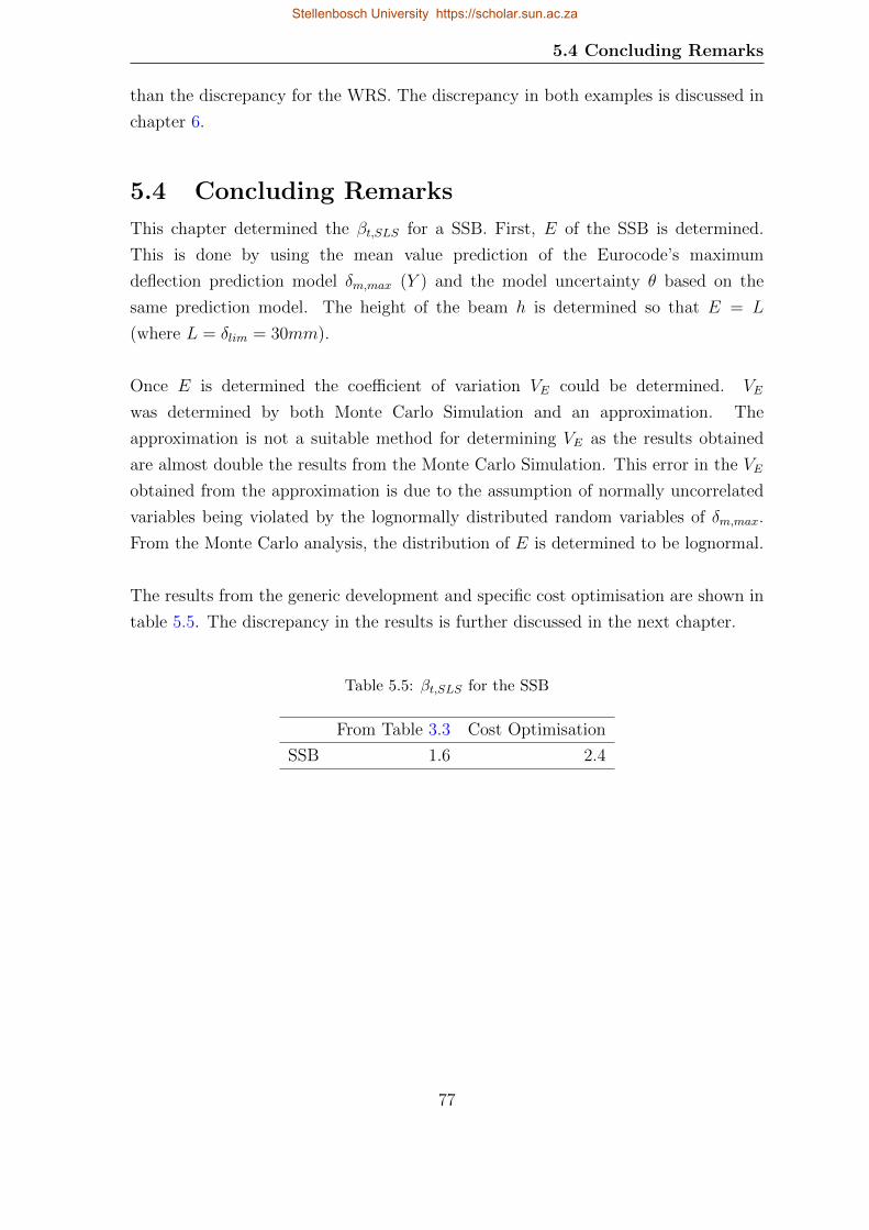
5.4 Concluding Remarks
than the discrepancy for the WRS. The discrepancy in both examples is discussed in
chapter 6.
5.4 Concluding Remarks
This chapter determined the βt,SLS for a SSB. First, E of the SSB is determined.
This is done by using the mean value prediction of the Eurocode’s maximum
deflection prediction model δm,max (Y ) and the model uncertainty θ based on the
same prediction model. The height of the beam h is determined so that E = L
(where L = δlim = 30mm).
Once E is determined the coefficient of variation VE could be determined. VE
was determined by both Monte Carlo Simulation and an approximation. The
approximation is not a suitable method for determining VE as the results obtained
are almost double the results from the Monte Carlo Simulation. This error in the VE
obtained from the approximation is due to the assumption of normally uncorrelated
variables being violated by the lognormally distributed random variables of δm,max.
From the Monte Carlo analysis, the distribution of E is determined to be lognormal.
The results from the generic development and specific cost optimisation are shown in
table 5.5. The discrepancy in the results is further discussed in the next chapter.
Table 5.5: βt,SLS for the SSB
From Table 3.3 Cost Optimisation
SSB 1.6 2.4
77
Stellenbosch University https://scholar.sun.ac.za
6. Discussion of the DiscrepancyA discrepancy in the βt,SLS obtained from the generic development (table 3.3) and
the βt,SLS determined from cost optimisation occurs for both the water retaining
structure, WRS, and simply supported beam, SSB. As this occurs for both crack
widths (WRS) and deflections (SSB), the discrepancy lies within the generic
simplifications for determining βt,SLS and not the specific cost optimisation of the
examples. In other words, it is assumed that the specific βt,SLS obtained from cost
optimisation of the specific structure is correct.
In this chapter, ”generic” refers to the generic limit state equation, decision parameter
d, and βt,SLS from table 3.3 while ”specific” refers to the specific limit state equation
of the examples, the decision parameters As and h, or the βt,SLS obtained from cost
optimisation of the example structure considered.
6.1 Investigation into the Cost Equation
The discrepancy between the generic βt,SLS and the specific βt,SLS is determined by
an investigation of the generic cost equation. The total costs of the structure which
are to be minimized is shown in equation 6.1. Equation 6.1 and its components are
discussed in chapter 3 (equation 3.1).
Ctot = C0 + C1d+ Cfpf (d) (6.1)
with d Decision parameter(s)
C0 Initial costs independent of d
C1 Costs of providing safety; dependent on d
Cf Failure costs
pf (d) Probability of failure as a function of d
C0 + C1d Construction costs
Cfpf (d) Expected failure costs
Deriving equation 6.1 with respect to d and setting it equal to zero results in
equation 6.2. When the derivative of Ctot is equal to zero, the costs are at a minimum
78
Stellenbosch University https://scholar.sun.ac.za

6.1 Investigation into the Cost Equation
and the corresponding d is the optimum decision parameter. This is the foundation
for the principles of cost optimisation. This is shown in figure 6.1.
∂Ctot∂d
= C1 + Cf∂pf (d)
∂d= 0
1 +CfC1
∂pf (d)
∂d= 0 (6.2)
From equation 6.2, it can be seen that the optimum decision parameter dopt and
corresponding βt,SLS are dependent on three components: the cost of providing safety
C1 per unit of d, the failure costs Cf , and the partial derivative ∂pf (d)/∂d of the
probability of failure pf (d) with respect to d. Changing any of these components
results in a shift in the dopt value.
Minimum Ctot
d
Costs
dopt
βt
β(d)
CtotC1d
Cfpf (d)β(d)
Figure 6.1: Concept of Cost Optimisation
The costs C1 influence the position of dopt based on the cost to increase d. Larger
values of C1 (expensive to increase d) imply that a safer structure is not economically
viable and therefore has a lower dopt and corresponding βt,SLS. The failure costs Cf ,
on the other hand, imply the opposite. Large values of Cf involve expensive costs
if failure does occur resulting in a larger dopt and βt,SLS. In other words, it is more
79
Stellenbosch University https://scholar.sun.ac.za

6.1 Investigation into the Cost Equation
economically viable to provide more safety.
The failure costs are also dependent on how efficient d is in decreasing the pf (d). For
an inefficient d, it is not economically viable to provide a safer structure as the pf (d)
does not change with increasing d, implying additional failure costs with little effect.
6.1.1 The Costs (C1 and Cf)
For the generic development, the cost of providing safety and the failure costs are
considered as a ratio. In the specific examples, Cf is quantified and C1 is determined
as the cost of providing the specific decision parameter. The total costs for the WRS
and SSB are shown in equations 6.3 and 6.4 respectively. For the WRS, the amount of
reinforcement As is the specific decision parameter and for the SSB, the height of the
beam h is the specific decision parameter. To determine the specific cost ratio (such
that the generic βt,SLS can be obtained from table 3.3), a relationship between the
specific costs of providing reinforcement or concrete with the generic costs of providing
safety is necessary.
Ctot = C0 + C1As + Cfpf (As) (6.3)
Ctot = C0 + C1h+ Cfpf (h) (6.4)
To map the specific costs of the examples to the generic cost ratio, the relationship
between the generic d and the specific decision parameters is considered. Since d = 1
implies that E = L, the amount of reinforcement AsL such that θwm,max = wlim or
height of the beam hL such that θδm,max = δlim is determined. The cost C1 associated
with providing this much reinforcement or concrete maps the specific C1 to the generic.
From these costs, the generic cost ratio can be determined and the genric βt,SLS can
be obtained for the specific examples. Based on how the costs are considered in the
specific examples, it appears that the discrepancy is not because of C1 or Cf . This
implies that the discrepancy is lies with in the∂pf (d)
∂dcomponent of the optimum
solution.
80
Stellenbosch University https://scholar.sun.ac.za
6.1 Investigation into the Cost Equation
6.1.2 The Decision Parameter and the Probability of
Failure pf(d)
The ∂pf (d)/∂d component depends on the efficiency of d to decrease the pf (d). For
the examples, the generic βt,SLS obtained from table 3.3 is lower than the specific
βt,SLS determined from cost optimisation. This implies that the generic d does not
decrease pf (d) as efficiently as the specific h decreases pf (h) or As decreases pf (As).
The decision parameter is linked to pf (d) through the action-resistance effect E of
the limit state equation. For the generic development, E is defined to be the inverse
of the decision parameter (for L = 1) as shown in equation 6.5. For both the WRS
and the SSB, there is not an explicit relationship between E and the chosen decision
parameter as shown in equations 6.6 and 6.7. In the specific cases, E is defined as a
function of the chosen decision parameter.
Generic:E =1
d(6.5)
WRS:E = θwm,max(As) (6.6)
SSB:E = θδm,max(h) (6.7)
with E Action-resistance effect
d Decision parameter of the generic structure
As Decision parameter of the WRS
h Decision parameter of the SSB
θ Model uncertainty
wm,max(As) Mean-maximum crack width as a function of As
δm,max(h) Mean-maximum deflection as a function of h
The decision parameter plays a role in how quickly C1 increases and how efficiently
pf (d) decreases. For the specific examples, the specific decision parameters were
determined such that E = L and d = 1. However, a linear relationship between
d and the specific decision parameters does not exist. Although d = 1 (E = L)
implies that As = AsL or h = hL, d = 2 (E = 0.5L) does not imply that
As = 2AsL or h = 2hL for the WRS and SSB respectively. This indicates that it is
more efficient to increase As or h than what is implied by d. This is shown in figure 6.2.
81
Stellenbosch University https://scholar.sun.ac.za
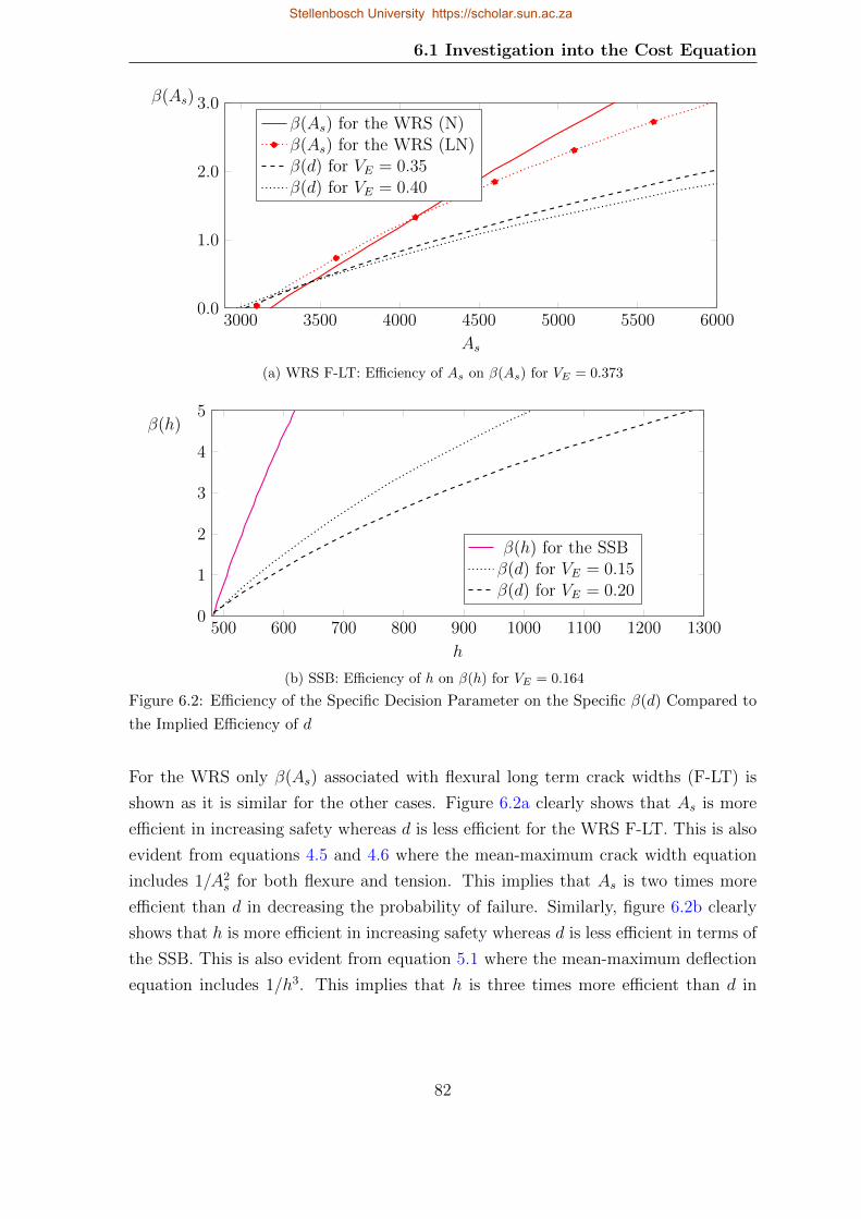
6.1 Investigation into the Cost Equation
3000 3500 4000 4500 5000 5500 60000.0
1.0
2.0
3.0
As
β(As)
β(As) for the WRS (N)β(As) for the WRS (LN)β(d) for VE = 0.35β(d) for VE = 0.40
(a) WRS F-LT: Efficiency of As on β(As) for VE = 0.373
500 600 700 800 900 1000 1100 1200 13000
1
2
3
4
5
h
β(h)
β(h) for the SSBβ(d) for VE = 0.15β(d) for VE = 0.20
(b) SSB: Efficiency of h on β(h) for VE = 0.164
Figure 6.2: Efficiency of the Specific Decision Parameter on the Specific β(d) Compared to
the Implied Efficiency of d
For the WRS only β(As) associated with flexural long term crack widths (F-LT) is
shown as it is similar for the other cases. Figure 6.2a clearly shows that As is more
efficient in increasing safety whereas d is less efficient for the WRS F-LT. This is also
evident from equations 4.5 and 4.6 where the mean-maximum crack width equation
includes 1/A2s for both flexure and tension. This implies that As is two times more
efficient than d in decreasing the probability of failure. Similarly, figure 6.2b clearly
shows that h is more efficient in increasing safety whereas d is less efficient in terms of
the SSB. This is also evident from equation 5.1 where the mean-maximum deflection
equation includes 1/h3. This implies that h is three times more efficient than d in
82
Stellenbosch University https://scholar.sun.ac.za

6.2 Proposed Solution
decreasing the probability of failure.
Due to the resulting inefficiency of the generic d on pf (d), a lower βt,SLS is determined
from the generic development than what is determined for the specific structure.
This is because a less efficient increase in the reliability of the structure results in a
lower optimum decision parameter as it is not economical to provide a higher level
of reliability. Although the assumption of E = 1/d is a reasonable assumption to
account for a range of structures, it is unconservative as it results in lower βt,SLS
values than what the reality of the specific examples suggest.
6.2 Proposed Solution
As the decision parameter does not account for the efficiency of the specific decision
parameters in decreasing pf (d), this discrepancy in βt,SLS needs to be accounted for.
The first solution would be to define a more efficient d in the generic development
of E. However, it may not be possible to sufficiently define d such that it takes into
account all serviceability prediction models, for example: E = 1/d2 may account
for the crack width prediction model but still be inefficient when compared to
the deflection model. On the other hand, the efficiency of the decision parameter
could be increased by adding some factor, for example: E = 1/d + 3. Further
investigations, into the decision parameters of specific examples and how efficiently
the decrease pf (d), are required for a range of serviceability prediction models (crack
widths, deflections, stresses, vibrations). Defining a more efficient d requires further
investigations and is out of the scope of this work.
The second solution would be to determine some efficiency parameter ϑ that takes
into account the discrepancy in the efficiency of pf (d) in the generic sense. This
efficiency parameter could be determined as a ratio of the partial derivative of the
optimum solution of the generic d to the partial derivative of the specific solution.
This is shown in equation 6.9.
83
Stellenbosch University https://scholar.sun.ac.za

6.2 Proposed Solution
1 +CfC1
∂pf (dG)
∂dG= 1 +
CfC1
∂pf (dS)
∂dS(6.8)
∂pf (dG)
∂dG= ϑ
∂pf (dS)
∂dS(6.9)
withCfC1
Cost ratio based on the generic framework
dG Decision parameter of the generic structure
dS Decision parameter of the specific structure
(for example As or h)
ϑ Efficiency parameter
If an efficiency parameter can be defined such that it takes into account the difference
in efficiency of the generic dG compared to the specific dS, the cost ratio of the
specific strucutre can be mapped to the cost ratio of the generic framework, as shown
in equation 6.10. The specific cost ratio is determined as discussed in the examples
(chapters 4 and 5).
CfC1
= ϑCfC1
(6.10)
withCfC1
Cost ratio based on the generic framework
ϑ Efficiency parameter
84
Stellenbosch University https://scholar.sun.ac.za

7. ConclusionThe current recommendation in ISO2394 for the target reliability of the serviceability
limit state is βt,SLS = 1.5. However, it is unclear how this βt,SLS was determined.
Specifically, for structures where the design is governed by the serviceability limit
state (SLS), the target values should be consistent with cost-optimal principles. The
goal of this project was to develop a generic framework to allow for easy estimation
of reliability-based cost-optimal βt,SLS values for different applications.
7.1 The Generic Framework
The target reliability values, for the serviceability limit state based on a generic
framework, were determined. The generic framework was established to perform
economic optimisation to establish βt,SLS from the same principles that βt,ULS were
calibrated. Cost optimisation was used to calculate the optimal βt,SLS for a range
of failure consequence classes, cost of safety measures, and variability characterising
different structures.
The principle of cost optimisation is to determine a reliability level that would
minimize the total costs of the structure. The total costs of a structure comprise of
the construction costs C0 + C1d plus the expected failure costs Cfpf (d). The cost
C1 is the cost of providing safety per unit of the decision parameter d. The failure
costs Cf are the costs incurred if there is serviceability failure. From the formulation
of the total costs, three components necessary for cost optimisation were identified:
the costs Cf and C1, the decision parameter d, and the reliability index β(d) as a
function of d.
A range of cost ratios Cf/C1 was identified as the best method to generically account
for the costs of the structure. Cost ratios from 0.5 up to 100 were considered. This
range was chosen to take into account the influences of the costs and consequences
associated with serviceability failure (failure costs Cf ) compared to costs of increasing
safety (costs per unit of d - C1).
85
Stellenbosch University https://scholar.sun.ac.za

7.1 The Generic Framework
To determine β(d), the first order reliability method (FORM) was identified as the
best technique to perform a reliability analysis. To conduct a FORM analysis the
limit state must be expressed as g = 0. From the limit state equation recommended
in the Eurocode, the variables were quantified in the generic sense. The design limit
L was assumed to be deterministic and the action-resistance effect E was identified
as a function of random variables. E was defined by the product of the mean value
prediction of the serviceability condition Y and the model uncertainty θ associated
with the same prediction model.
For the generic structure it was determined that assigning E as random variable
would be sufficient for the reliability analysis. The range for the mean values of
the action-resistance effect µE was determined based on the relationship established
between µE and the decision parameter d. From the generic limit state equation, µE is
inversely proportional to d. The coefficient of variation VE was varied parametrically
to account for a wide range of structures. The range VE = [0.05 − 0.50] was chosen
to account for the low variability of deflections and stresses to the high variability of
cracking. Once this range was established, a reliability analysis was performed using
FORM to determine the β(d) values.
7.1.1 Conclusion of βt,SLS for the Generic Structure
From the range of cost ratios and β(d) values for the range of VE, economic
optimisation was conducted to determine a parametric table of βt,SLS values. The
βt,SLS values obtained are shown in table 7.1.
Table 7.1 covered a large range of structures for a range of serviceability conditions
in a generic sense. It is expected that crack widths are covered by the range of
VE = [0.15− 0.45], depending on the degree of uncertainty associated with the model
factor, and anticipated that for deflections and stresses the range VE = [0.05 − 0.25]
would represent the βt,SLS for these structures. From this the necessity of such a
large range for VE is clear and reducing the range would result in some structures
not being suitably represented. For a specific structure, βt,SLS can be determined
based on the costs of increasing safety and the cost of failure for the specific structure
combined with the variability of the action-resistance effect.
86
Stellenbosch University https://scholar.sun.ac.za

7.2 The Applications
Table 7.1: βt,SLS for a One Year Reference Period
Cf/C1
VE 0.5 0.8 1.0 1.5 2.0 4.0 10 20 50 100
0.50 0.0 0.0 0.0 0.5 0.7 1.2 1.7 2.0 2.3 2.6
0.45 0.0 0.0 0.0 0.6 0.8 1.3 1.8 2.1 2.4 2.6
0.40 -0.1 -0.1 0.2 0.7 0.9 1.4 1.8 2.1 2.5 2.7
0.35 -0.1 0.0 0.4 0.8 1.1 1.5 1.9 2.2 2.6 2.8
0.30 -0.2 0.3 0.6 1.0 1.2 1.6 2.0 2.3 2.6 2.9
0.25 -0.3 0.5 0.8 1.1 1.3 1.7 2.1 2.4 2.7 3.0
0.20 0.1 0.8 1.0 1.3 1.5 1.9 2.3 2.5 2.8 3.1
0.15 0.7 1.1 1.3 1.5 1.7 2.0 2.4 2.7 3.0 3.2
0.10 1.1 1.5 1.5 1.8 2.0 2.3 2.6 2.8 3.1 3.4
0.05 1.6 1.9 1.9 2.1 2.3 2.6 3.0 3.2 3.3 3.7
7.2 The Applications
A study into the application of table 7.1 was conducted for three structures. Two
water retaining structures (WRS), for the prediction of the crack width, and one
simply supported beam (SSB), for the prediction of the maximum deflection,
were investigated. βt,SLS was obtained from table 7.1 and calculated through cost
optimisation for the three structures. The target values from the two methods were
compared to ensure that the results were approximately equivalent.
E for the specific structures was calculated. For the WRS the amount of reinforcement
AsL was determined so that µE = L (where L = wlim = 0.2mm). The amount of
reinforcement required As is governed by long term flexural and tensile loading for
the two investigated structures. For the SSB, the beam’s height hL was determined
so that µE = L (where L = δlim = 30mm).
The coefficient of variation VE was determined by both Monte Carlo Simulation
(MCS) and a mathematical approximation that assumes the input variables are
normally distributed. The approximation resulted in a similar VE to the VE obtained
from the MCS for the WRS. However, for the SSB, the VE from the approximation
was almost double the VE from the MCS. This was due to the lognormal distribution
87
Stellenbosch University https://scholar.sun.ac.za
7.2 The Applications
of the random variables of the action-resistance effect violating the assumptions on
which the approximation is based.
From the MCS, the distribution of E was determined. For the WRS, θ was
investigated as normal (N) and lognormal (LN). This resulted in corresponding N
and LN distributions of E. A LN distribution was fit to E of the SSB. VE was
calculated as 0.373 and 0.332 for flexure and tension of the WRS respectively. For
the SSB a smaller VE = 0.164 was calculated.
The next step was to quantify the costs for the specific structures. The failure
costs Cf were assumed to be the cost of providing liquid-tight lining for the WRS
(Cf = R1500/m2) and the cost to strengthen the beam for the SSB (Cf = R6000).
It was assumed that there are no indirect failure costs for the two examples. The
cost of providing safety C1 is dependent on d in the generic framework. Since d = 1
implies E = L, the cost C1 is calculated to be the cost of providing AsL for the WRS
and hL for the SSB. The cost ratios were quantified as Cf/C1 = 5.9 and 4.5 for
WRS 1 and WRS 2 flexural cracking respectively. For tension, Cf/C1 = 6.2 for both
WRS 1 and 2 as AsL = 3000mm2 for both structures. For the SSB the cost ratio was
quantified as Cf/C1 = 1.9.
βt,SLS for the specific examples was then obtained from the generic framework
(table 7.1). These target values βt,SLS are compared to the βt,SLS obtained from
cost optimisation of the specific structures. The results from the cost optimisation
did not consolidate with βt,SLS values obtained from the generic framework for both
the WRS and SSB. The results from the applications are shown in table 7.2.
88
Stellenbosch University https://scholar.sun.ac.za

7.2 The Applications
Table 7.2: Summary of βt,SLS for the Applications
Cost Optimisation
Table 7.1 Normal Lognormal
F-LT WRS 1 1.6 2.2 1.9
WRS 2 1.5 2.1 1.9
T-LT WRS 1 1.7 2.2 2.1
WRS2 1.7 2.3 2.2
SSB 1.6 - 2.4
7.2.1 Conclusion of the Generic βt,SLS based on the
Applications
As observed in table 7.2, it is evident that there is a discrepancy between the generic
framework for βt,SLS and the specific βt,SLS obtained from cost optimisation of the
examples. The βt,SLS read from table 7.1 underestimate the βt,SLS of the specific
structures.
It was anticipated that the assumption of E, having a lognormal distribution for the
generic framework, would not always hold for a specific structure. For a structure
where E has a non-lognormal distribution, the generic βt,SLS may not sufficiently
account for the reliability of the structure. The WRS was investigated to have both a
normal and lognormal distribution for both flexural and tensile cracking. For flexure
(F-LT) the difference in the results from cost optimisation for a lognormally and
normally distributed E is approximately ∆βt,SLS ≈ 0.2. Tension (T-LT) on the other
hand has a negligible difference of ∆βt,SLS ≈ 0.1. However, from the results shown in
table 7.2 it is evident that the distribution of E is not the reason for the discrepancy
in the results.
The coefficient of variation VE of the action-resistance effect of the specific structures
is sufficiently covered by the range of VE considered in the generic development.
This implies that the discrepancy lies within the cost optimisation component of the
generic framework. The partial derivative of the total costs with respect to d was
investigated because when equal to zero, the optimum occurs. Three components
89
Stellenbosch University https://scholar.sun.ac.za

7.3 Recommendations
were then identified to have an influence on the optimum; C1, Cf and the partial
derivative ∂pf (d)/∂d of the probability of failure pf (d) with respect to d.
The first and second components, C1 and Cf , were accounted for in the generic
framework through the cost ratio Cf/C1. For the specific examples, the costs of
providing one unit of d was determined by calculating the cost associated with
providing reinforcement or concrete such that E = L. It was concluded that the
discrepancy was not a result of the cost components.
The third component which influences the position of the optimum is ∂pf (d)/∂d .
The position of the optimum depends on the efficiency of d to decrease pf (d). It was
identified that there was non-linear relationship between d of the generic framework
and the specific decision parameters (As or h). Investigation into this non-linear
relationship revealed that it was more efficient to increase As or h than what was
implied by d. This resulted in higher target values for the examples from cost
optimisation of the specific structures than what was determined from the generic
framework.
The generic model is unconservative in the recommendations of βt,SLS. However,
the generic development set out by this thesis provides a suitable framework for
determining βt,SLS. As the generic model oversimplifies the SLS, further investigations
into improving the generic framework should be conducted.
7.3 Recommendations
The generic framework and corresponding βt,SLS values provide a reasonable
foundation for the reliability assessment of concrete structures governed by the SLS.
This section lists the recommendations for further research into the target reliability
related with SLS design.
This thesis identified a discrepancy in the the target values obtained from the
generic framework and the cost optimisation of the specific example structures. The
discrepancy is due to the lower efficiency of the decision parameter to decrease the
probability of failure pf (d) in the generic case compared to the efficiency of decision
parameters to do the same in the specific examples. Further investigations into
90
Stellenbosch University https://scholar.sun.ac.za
7.3 Recommendations
increasing the efficiency of the generic decision parameter is necessary. However, it
may not be possible to determine a generic decision parameter which accounts for
different efficiencies of specific decision parameters of various SLS criteria. If this is
the case, it may be necessary to determine an efficiency parameter to account for the
discrepancy in the efficiency of the generic decision parameter.
The generic decision parameter in this thesis is based on the generalisations made
by Rackwitz [38] for βt,ULS. The question arises as to whether or not the generic
decision parameter efficiently decreases the pf (d) for the ULS. Reliability-based cost
optimisation should be performed for the ULS for a range of example structures to
determine how well current target values represent optimal design for these structures.
This thesis assumed a lognormal distribution of the action-resistance effect. This
choice reflects the assumption that both resistance and load effect have a lower
bound at zero. However, the skewness implied by the two parameter lognormal
assumption may be too high, particularly for cases where model uncertainty with
a normal distribution dominates. Another scenario where the distribution may be
different is when the variable load is dominating and has a Gumbel rather than
lognormal distribution. It may be useful to assess the influence of distribution type
on the assessed optimal βt,SLS values.
91
Stellenbosch University https://scholar.sun.ac.za

References[1] E. Aktas, F. Moses, and M. Ghosn. “Cost and safety optimization of structural
design specifications”. In: Reliability Engineering & System Safety 73.3 (2001),
pp. 205–212 (cit. on p. 24).
[2] A.-S. Ang and D. De Leon. “Determination of optimal target reliabilities
for design and upgrading of structures”. In: Structural Safety 19.1 (1997),
pp. 91–103 (cit. on p. 23).
[3] T. Braml, A. Taffe, S. Feistkorn, and O. Wurzer. “Assessment of Existing
Structures using Probabilistic Analysis Methods in Combination with
Nondestructive Testing Methods”. In: Structural Engineering International 23.4
(2013), pp. 376–385 (cit. on p. 6).
[4] V. Cervenka, J. Markova, J. Mlcoch, A. Perez Caldentey, T. Sajdlova, and M.
Sykora. “Uncertainties of Crack Width Models” (cit. on pp. 10, 11).
[5] S.-K. Choi, R. A. Canfield, and R. V. Grandhi. “Reliability-based Structural
Design”. In: Reliability-based Structural Design. Springer, Jan. 1, 2007. isbn:
978-1-84628-444-1 (cit. on pp. 16, 17, 51).
[6] O. Ditlevsen and H. O. Madsen. Structural reliability methods. Vol. 178. Wiley
New York, 1996 (cit. on pp. 6, 12, 51).
[7] Eurocode - Basis of Structural Design. Brussels, 2002 (cit. on pp. 6, 12–15, 17,
27).
[8] Eurocode 2 - Design of Concrete Structures Part 1-1. Brussels, 2004 (cit. on
pp. 43–45, 68–70).
[9] Eurocode 2 - Design of Concrete Structures Part 3: Liquid Retaining and
Containment Structures. Brussels, 2006 (cit. on p. 43).
[10] M. Faber and J. Sφrensen. “Reliability Based Code Calibration”. In: Joint
Committee on Structural Safety (2002) (cit. on pp. 7, 28).
[11] R. Gilbert. “The serviceability limit states in reinforced concrete design”. In:
Procedia Engineering 14 (2011), pp. 385–395 (cit. on pp. 10, 11).
[12] Handbook 1 - Basis of Structural Design. Leonardo da Vinci Pilot Project, 2004
(cit. on p. 6).
[13] Handbook 2 - Reliability Backgrounds. Leonardo da Vinci Pilot Project, 2005
(cit. on pp. 6, 12, 15–17, 30, 51, 57).
92
Stellenbosch University https://scholar.sun.ac.za
REFERENCES
[14] M. Holicky, J. Retief, and J. Wium. “Probabilistic design for cracking of concrete
structures”. In: Proceedings of the 7th International Probabilistic Workshop:
25-26 November 2009, Delft, The Netherlands. Dirk Proske Verlag. 2009, p. 87
(cit. on p. 53).
[15] M. Holicky. “Specification of the Target Reliability Level”. In: Stochastic Models
in Reliability Engineering, Life Science and Operations Management (SMRLO),
2016 Second International Symposium on. IEEE. 2016, pp. 104–108 (cit. on
p. 31).
[16] M. Holicky. “The target reliability and design working life”. In: Safety and
Security Engineering (2011) (cit. on p. 25).
[17] M. Holicky. “Optimisation of the target reliability for temporary structures”.
In: Civil Engineering and Environmental Systems 30.2 (2013), pp. 87–96 (cit. on
p. 25).
[18] M. Holicky. Reliability analysis for structural design. AFRICAN SUN MeDIA,
2009 (cit. on pp. 9–11, 15–18, 23, 53, 72).
[19] M. Holicky, D. Diamantidis, and M. Sykora. “Determination of target safety for
structures”. In: (2015) (cit. on pp. 21–24).
[20] M. Holicky, J. V. Retief, and M. Sykora. “Assessment of Model Uncertainties
for Structural Resistance”. In: Probabilistic Engineering Mechanics 45 (2016),
pp. 188–197 (cit. on pp. 7–9, 28, 29).
[21] D. Honfi, A. Martensson, and S. Thelandersson. “Reliability of beams according
to Eurocodes in serviceability limit state”. In: Engineering Structures 35 (2012),
pp. 48–54 (cit. on pp. 10, 11, 68, 72).
[22] IPM Steel. Personal communication. via Telephone. Sept. 2017 (cit. on p. 58).
[23] ISO2394(1998) - General Principles on Reliability for Structures. Second. ISO.
2012 (cit. on pp. 1, 6, 13–15, 21).
[24] ISO2394(2015) - General Principles on Reliability for Structures. Third. ISO.
2015 (cit. on pp. 7, 9, 12).
[25] Joint Committee on Structural Safety. “JCSS, Probabilistic Model Code”. In:
Zurich, Switzerland (2001) (cit. on pp. 6, 7, 12–15, 24, 25, 40, 53).
[26] Joint Committee on Structural Safety. “JCSS, Probabilistic Model Code Part
2: Load Models”. In: Zurich, Switzerland (2001) (cit. on p. 72).
93
Stellenbosch University https://scholar.sun.ac.za

REFERENCES
[27] Joint Committee on Structural Safety. “JCSS, Probabilistic Model Code Part
3: Material Properties”. In: Zurich, Switzerland (2001) (cit. on p. 53).
[28] J. Kanda and H. Shah. “Engineering role in failure cost evaluation for buildings”.
In: Structural Safety 19.1 (1997), pp. 79–90 (cit. on p. 40).
[29] Lafarge 2014 Price List. https://documents.tips/documents/lafarge-2014-pricelist.html
(cit. on pp. 73, 76).
[30] J. Markova and M. Sykora. “Risk, Reliability and Safety: Innovating Theory
and Practice”. In: ed. by L. Walls, M. Revie, and T. Bedford. Taylor and
Francis Group, London, 2017. Chap. Uncertainties in Crack Width Verification
of Reinforced Concrete Structures (cit. on pp. 10, 11, 40, 53).
[31] C. McLeod, C. Barnardo-Vijloen, and J. Retief. “Quantification of model
uncertainty of EN1992 crack width prediction model”. In: Insights and
Innovations in Structural Engineering, Mechanics and Computation (2016),
pp. 1349–1354 (cit. on p. 40).
[32] C. McLeod, C. Vijloen, and J. Retief. “Determining Model Uncertainty
Associated with Concrete Crack Models for Members in Flexure”. In: 15th
International Probabilistic Workshop. 2017 (cit. on pp. 46, 47, 53).
[33] C. McLeod, C. Vijloen, and J. Retief. “Determining Model Uncertainty
Associated with Concrete Crack Models for Members in Tension”. In: 15th
International Probabilistic Workshop. 2017 (cit. on pp. 46, 47, 53).
[34] C. McLeod. Personal communication. via Email. May 2017 (cit. on p. 49).
[35] C. H. McLeod. “Investigation into cracking in reinforced concrete
water-retaining structures”. MA thesis. Stellenbosch: Stellenbosch University,
2013 (cit. on pp. 7, 10, 46, 53).
[36] R. Melchers. Structural Reliability Analysis and Prediction. 2nd. John Wiley
and Sons Ltd, 1999 (cit. on pp. 7, 28, 57).
[37] Q. Quan and Z. Gengwei. “Calibration of Reliability Index of RC Beams
for Serviceability Limit State of Maximum Crack Width”. In: Reliability
Engineering and System Safety 75 (2002), pp. 359–366 (cit. on pp. 10, 11).
[38] R. Rackwitz. “Optimization - the basis of code-making and reliability
verification”. In: Structural safety 22.1 (2000), pp. 27–60 (cit. on pp. 23, 29,
31, 91).
[39] M. A. El-Reedy. Reinforced concrete structural reliability. CRC Press, 2012 (cit.
on pp. 51, 52).
94
Stellenbosch University https://scholar.sun.ac.za

REFERENCES
[40] @RISK software. http://www.palisade.com/risk/. Palisade (cit. on p. 52).
[41] RT software. http://www.inrisk.ubc.ca/software/. InRisk Department of Civil
Engineering University British Colombia (cit. on pp. 30, 61, 75).
[42] C. Smit and C. Barnardo-Viljoen. “Reliability based optimisation of concrete
structural components”. In: IPW11: The 11th International Probabilistic
Workshop. (Brno). 2013, pp. 391–404 (cit. on pp. 47, 69).
[43] R. Steenbergen, M. Sykora, D. Diamantidis, M. Holicky, and A. Vrouwenvelder.
“Target reliability levels for assessment of existing structures based on economic
optimization and human safety criteria”. In: Structural Concrete 16 (2015),
pp. 323–332 (cit. on pp. 22, 24).
[44] M. Sykora, D. Diamantidis, M. Holicky, and K. Jung. “Target reliability levels
for assessment of existing structures considering economic and societal aspects”.
In: Proc. Fourth International Symposium on Life-Cycle Civil Engineering
IALCCE. 2014, pp. 838–845 (cit. on pp. 22, 23).
[45] M. Sykora and M. Holicky. “Target reliability levels for the assessment of
existing structures–case study”. In: Life-Cycle and Sustainability of Civil
Infrastructure Systems: Proceedings of the Third International Symposium on
Life-Cycle Civil Engineering (IALCCE’12), Vienna, Austria, October 3-6, 2012.
CRC Press. 2012, p. 189 (cit. on p. 24).
[46] M. Sykora, D. Diamantidis, and M. Holicky. Target Reliability for Existing Civil
Engineering Systems. Tech. rep. Klokner Institute Czech Technical University
in Prague Prague, Czech Republic, 2016 (cit. on pp. 21, 22, 24).
[47] M. Sykora, D. Diamantidis, M. Holicky, and K. Jung. “Target reliability for
existing structures considering economic and societal aspects”. In: Structure
and Infrastructure Engineering: Maintenance, Management, Life-Cycle Design
and Performance (2016) (cit. on pp. 25, 59).
[48] M. Sykora, M. Holicky, and D. Diamantidis. “Target Reliability for Existing
Civil Engineering Systems”. In: 2016 Second International Symposium on
Stochastic Models in Reliability Engineering, Life Science and Operations
Management (SMRLO). IEEE. 2016, pp. 109–114 (cit. on p. 22).
[49] M. Sykora, M. Holicky, and J. Markova. “Target reliability levels for assessment
of existing structures”. In: Applications of Statistics and Probability in Civil
Engineering (2011), p. 311 (cit. on p. 23).
95
Stellenbosch University https://scholar.sun.ac.za

REFERENCES
[50] T. Vrouwenvelder. “Developments towards full probabilistic design codes”. In:
Structural Safety (2002) (cit. on p. 25).
[51] R. Walls. Advanced Design of Concrete Strucutres - Design for Serviceability.
Stellenbosch University. Advanced Design of Concrete Strucutres Course Notes.
Sept. 2016 (cit. on p. 68).
96
Stellenbosch University https://scholar.sun.ac.za
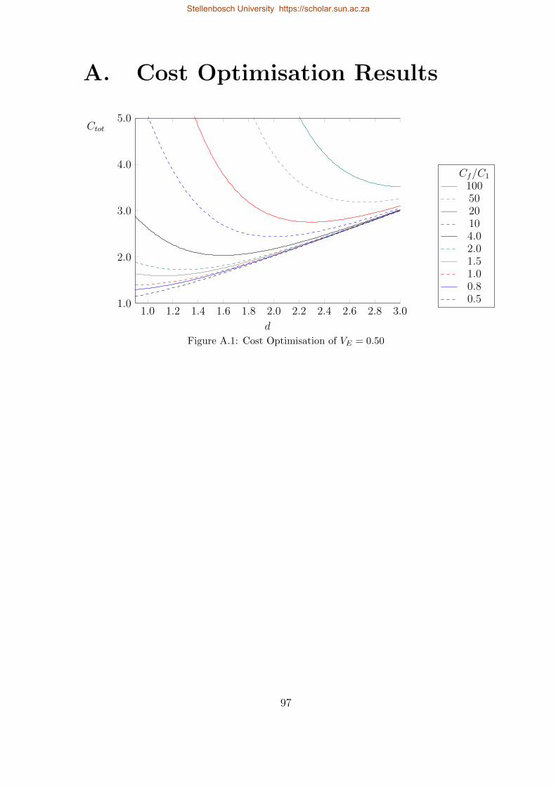
A. Cost Optimisation Results
1.0 1.2 1.4 1.6 1.8 2.0 2.2 2.4 2.6 2.8 3.01.0
2.0
3.0
4.0
5.0
d
Ctot
Cf/C1
1005020104.02.01.51.00.80.5
Figure A.1: Cost Optimisation of VE = 0.50
97
Stellenbosch University https://scholar.sun.ac.za

1.0 1.2 1.4 1.6 1.8 2.0 2.2 2.4 2.6 2.8 3.01.0
2.0
3.0
4.0
5.0
d
Ctot
Cf/C1
1005020104.02.01.51.00.80.5−1.0
0.0
1.0
2.0
3.0
4.0β(d)
Figure A.2: Cost Optimisation of VE = 0.45
1.0 1.2 1.4 1.6 1.8 2.0 2.2 2.4 2.6 2.8 3.01.0
2.0
3.0
4.0
5.0
d
Ctot
Cf/C1
1005020104.02.01.51.00.80.5−1.0
0.0
1.0
2.0
3.0
4.0β(d)
Figure A.3: Cost Optimisation of VE = 0.40
98
Stellenbosch University https://scholar.sun.ac.za

1.0 1.2 1.4 1.6 1.8 2.0 2.2 2.4 2.6 2.8 3.01.0
2.0
3.0
4.0
5.0
d
Ctot
Cf/C1
1005020104.02.01.51.00.80.5−1.0
0.0
1.0
2.0
3.0
4.0β(d)
Figure A.4: Cost Optimisation of VE = 0.35
1.0 1.2 1.4 1.6 1.8 2.0 2.2 2.4 2.6 2.8 3.01.0
2.0
3.0
4.0
5.0
d
Ctot
Cf/C1
1005020104.02.01.51.00.80.5−1.0
0.0
1.0
2.0
3.0
4.0β(d)
Figure A.5: Cost Optimisation of VE = 0.30
99
Stellenbosch University https://scholar.sun.ac.za
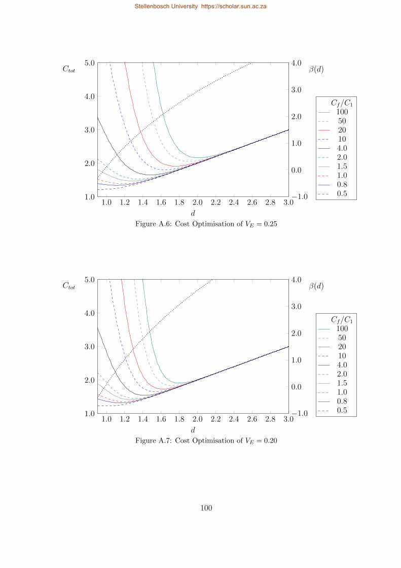
1.0 1.2 1.4 1.6 1.8 2.0 2.2 2.4 2.6 2.8 3.01.0
2.0
3.0
4.0
5.0
d
Ctot
Cf/C1
1005020104.02.01.51.00.80.5−1.0
0.0
1.0
2.0
3.0
4.0β(d)
Figure A.6: Cost Optimisation of VE = 0.25
1.0 1.2 1.4 1.6 1.8 2.0 2.2 2.4 2.6 2.8 3.01.0
2.0
3.0
4.0
5.0
d
Ctot
Cf/C1
1005020104.02.01.51.00.80.5−1.0
0.0
1.0
2.0
3.0
4.0β(d)
Figure A.7: Cost Optimisation of VE = 0.20
100
Stellenbosch University https://scholar.sun.ac.za
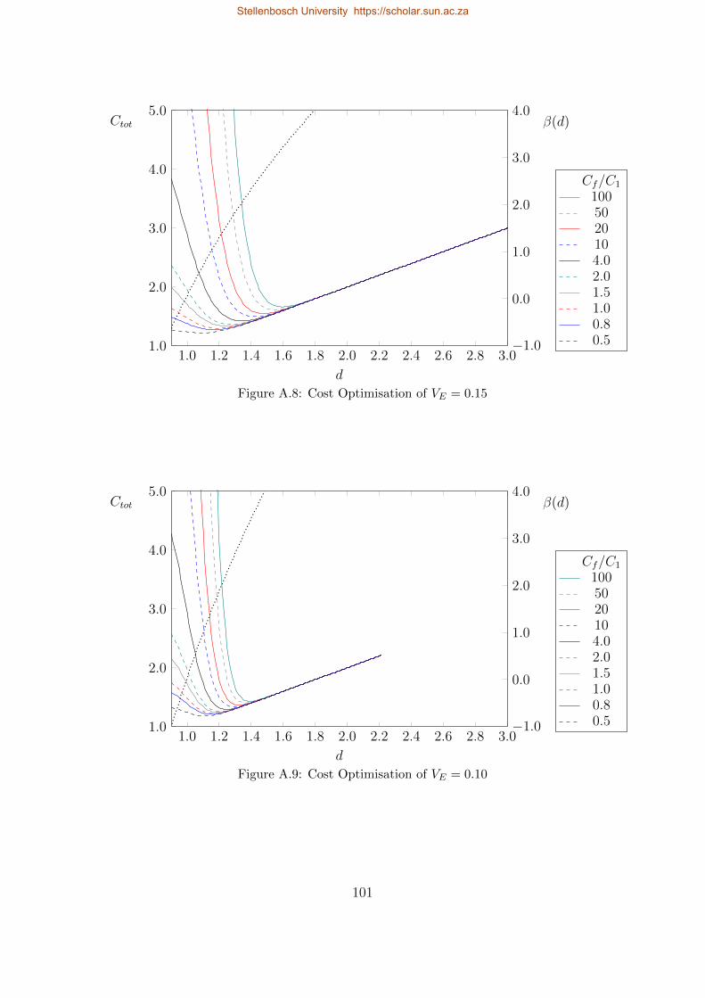
1.0 1.2 1.4 1.6 1.8 2.0 2.2 2.4 2.6 2.8 3.01.0
2.0
3.0
4.0
5.0
d
Ctot
Cf/C1
1005020104.02.01.51.00.80.5−1.0
0.0
1.0
2.0
3.0
4.0β(d)
Figure A.8: Cost Optimisation of VE = 0.15
1.0 1.2 1.4 1.6 1.8 2.0 2.2 2.4 2.6 2.8 3.01.0
2.0
3.0
4.0
5.0
d
Ctot
Cf/C1
1005020104.02.01.51.00.80.5−1.0
0.0
1.0
2.0
3.0
4.0β(d)
Figure A.9: Cost Optimisation of VE = 0.10
101
Stellenbosch University https://scholar.sun.ac.za

1.0 1.2 1.4 1.6 1.8 2.0 2.2 2.4 2.6 2.8 3.01.0
2.0
3.0
4.0
5.0
d
Ctot
Cf/C1
1005020104.02.01.51.00.80.5−1.0
0.0
1.0
2.0
3.0
4.0β(d)
Figure A.10: Cost Optimisation of VE = 0.05
1.0 1.2 1.4 1.6 1.8 2.0 2.2 2.4 2.6 2.8 3.01.0
2.0
3.0
4.0
5.0
d
Ctot
VE0.500.450.400.350.300.250.200.150.100.05
Figure A.11: Cost Optimisation of Cf/C1 = 0.5
102
Stellenbosch University https://scholar.sun.ac.za
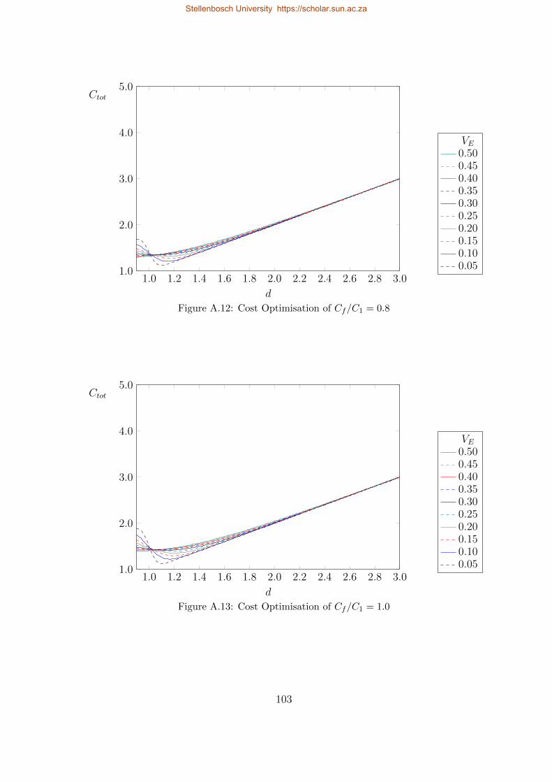
1.0 1.2 1.4 1.6 1.8 2.0 2.2 2.4 2.6 2.8 3.01.0
2.0
3.0
4.0
5.0
d
Ctot
VE0.500.450.400.350.300.250.200.150.100.05
Figure A.12: Cost Optimisation of Cf/C1 = 0.8
1.0 1.2 1.4 1.6 1.8 2.0 2.2 2.4 2.6 2.8 3.01.0
2.0
3.0
4.0
5.0
d
Ctot
VE0.500.450.400.350.300.250.200.150.100.05
Figure A.13: Cost Optimisation of Cf/C1 = 1.0
103
Stellenbosch University https://scholar.sun.ac.za

1.0 1.2 1.4 1.6 1.8 2.0 2.2 2.4 2.6 2.8 3.01.0
2.0
3.0
4.0
5.0
d
Ctot
VE0.500.450.400.350.300.250.200.150.100.05
Figure A.14: Cost Optimisation of Cf/C1 = 1.5
1.0 1.2 1.4 1.6 1.8 2.0 2.2 2.4 2.6 2.8 3.01.0
2.0
3.0
4.0
5.0
d
Ctot
VE0.500.450.400.350.300.250.200.150.100.05
Figure A.15: Cost Optimisation of Cf/C1 = 2.0
104
Stellenbosch University https://scholar.sun.ac.za
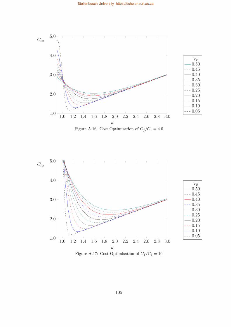
1.0 1.2 1.4 1.6 1.8 2.0 2.2 2.4 2.6 2.8 3.01.0
2.0
3.0
4.0
5.0
d
Ctot
VE0.500.450.400.350.300.250.200.150.100.05
Figure A.16: Cost Optimisation of Cf/C1 = 4.0
1.0 1.2 1.4 1.6 1.8 2.0 2.2 2.4 2.6 2.8 3.01.0
2.0
3.0
4.0
5.0
d
Ctot
VE0.500.450.400.350.300.250.200.150.100.05
Figure A.17: Cost Optimisation of Cf/C1 = 10
105
Stellenbosch University https://scholar.sun.ac.za

1.0 1.2 1.4 1.6 1.8 2.0 2.2 2.4 2.6 2.8 3.01.0
2.0
3.0
4.0
5.0
d
Ctot
VE0.500.450.400.350.300.250.200.150.100.05
Figure A.18: Cost Optimisation of Cf/C1 = 20
1.0 1.2 1.4 1.6 1.8 2.0 2.2 2.4 2.6 2.8 3.01.0
2.0
3.0
4.0
5.0
d
Ctot
VE0.500.450.400.350.300.250.200.150.100.05
Figure A.19: Cost Optimisation of Cf/C1 = 50
106
Stellenbosch University https://scholar.sun.ac.za

1.0 1.2 1.4 1.6 1.8 2.0 2.2 2.4 2.6 2.8 3.01.0
2.0
3.0
4.0
5.0
d
Ctot
VE0.500.450.400.350.300.250.200.150.100.05
Figure A.20: Cost Optimisation of Cf/C1 = 100
107
Stellenbosch University https://scholar.sun.ac.za

B. WRS Crack WidthsExcel spreadsheets used to calculate wm,max.
108
Stellenbosch University https://scholar.sun.ac.za
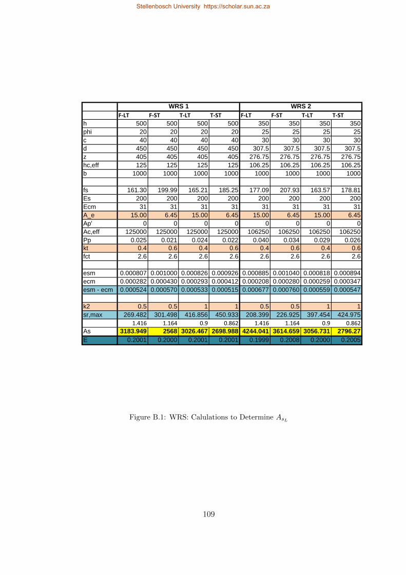
F‐LT F‐ST T‐LT T‐ST F‐LT F‐ST T‐LT T‐ST
h 500 500 500 500 350 350 350 350phi 20 20 20 20 25 25 25 25c 40 40 40 40 30 30 30 30d 450 450 450 450 307.5 307.5 307.5 307.5z 405 405 405 405 276.75 276.75 276.75 276.75hc,eff 125 125 125 125 106.25 106.25 106.25 106.25b 1000 1000 1000 1000 1000 1000 1000 1000
fs 161.30 199.99 165.21 185.25 177.09 207.93 163.57 178.81Es 200 200 200 200 200 200 200 200Ecm 31 31 31 31 31 31 31 31A_e 15.00 6.45 15.00 6.45 15.00 6.45 15.00 6.45Ap' 0 0 0 0 0 0 0 0Ac,eff 125000 125000 125000 125000 106250 106250 106250 106250Pp 0.025 0.021 0.024 0.022 0.040 0.034 0.029 0.026kt 0.4 0.6 0.4 0.6 0.4 0.6 0.4 0.6fct 2.6 2.6 2.6 2.6 2.6 2.6 2.6 2.6
esm 0.000807 0.001000 0.000826 0.000926 0.000885 0.001040 0.000818 0.000894ecm 0.000282 0.000430 0.000293 0.000412 0.000208 0.000280 0.000259 0.000347esm - ecm 0.000524 0.000570 0.000533 0.000515 0.000677 0.000760 0.000559 0.000547
k2 0.5 0.5 1 1 0.5 0.5 1 1sr,max 269.482 301.498 416.856 450.933 208.399 226.925 397.454 424.975
1.416 1.164 0.9 0.862 1.416 1.164 0.9 0.862
As 3183.949 2568 3026.467 2698.988 4244.041 3614.659 3056.731 2796.27E 0.2001 0.2000 0.2001 0.2001 0.1999 0.2008 0.2000 0.2005
WRS 1 WRS 2
Figure B.1: WRS: Calulations to Determine AsL
109
Stellenbosch University https://scholar.sun.ac.za

t = h 500.000 mm fcu 30.000 MPa phi 20.000b = D 20.000 m fy 450.000 MPa cover 40.000H 5.000 m As 314.1592654
V 1570.796 m^3 y_water 10.000 kN/m^2Ms 208.000
w_lim 0.2 mmAs 2900 3000 3100 3200 3300 3400 3500 3600 3700 3800 3900 4000 4100 4200 4300 4400 4500 4600 4700 4800h 500 500 500 500 500 500 500 500 500 500 500 500 500 500 500 500 500 500 500 500phi 20 20 20 20 20 20 20 20 20 20 20 20 20 20 20 20 20 20 20 20c 40 40 40 40 40 40 40 40 40 40 40 40 40 40 40 40 40 40 40 40d 450 450 450 450 450 450 450 450 450 450 450 450 450 450 450 450 450 450 450 450z 405 405 405 405 405 405 405 405 405 405 405 405 405 405 405 405 405 405 405 405hc,eff 125 125 125 125 125 125 125 125 125 125 125 125 125 125 125 125 125 125 125 125b 1000 1000 1000 1000 1000 1000 1000 1000 1000 1000 1000 1000 1000 1000 1000 1000 1000 1000 1000 1000
fs 177.10 171.19 165.67 160.49 155.63 151.05 146.74 142.66 138.81 135.15 131.69 128.40 125.26 122.28 119.44 116.72 114.13 111.65 109.27 107.00Es 200 200 200 200 200 200 200 200 200 200 200 200 200 200 200 200 200 200 200 200Ecm 31 31 31 31 31 31 31 31 31 31 31 31 31 31 31 31 31 31 31 31A_e 15.00 15.00 15.00 15.00 15.00 15.00 15.00 15.00 15.00 15.00 15.00 15.00 15.00 15.00 15.00 15.00 15.00 15.00 15.00 15.00Ap' 0 0 0 0 0 0 0 0 0 0 0 0 0 0 0 0 0 0 0 0Ac,eff 125000 125000 125000 125000 125000 125000 125000 125000 125000 125000 125000 125000 125000 125000 125000 125000 125000 125000 125000 125000Pp 0.023 0.024 0.025 0.026 0.026 0.027 0.028 0.029 0.030 0.030 0.031 0.032 0.033 0.034 0.034 0.035 0.036 0.037 0.038 0.038kt 0.4 0.4 0.4 0.4 0.4 0.4 0.4 0.4 0.4 0.4 0.4 0.4 0.4 0.4 0.4 0.4 0.4 0.4 0.4 0.4fct 2.6 2.6 2.6 2.6 2.6 2.6 2.6 2.6 2.6 2.6 2.6 2.6 2.6 2.6 2.6 2.6 2.6 2.6 2.6 2.6
esm 0.000885 0.000856 0.000828 0.000802 0.000778 0.000755 0.000734 0.000713 0.000694 0.000676 0.000658 0.000642 0.000626 0.000611 0.000597 0.000584 0.000571 0.000558 0.000546 0.000535ecm 0.000302 0.000295 0.000288 0.000281 0.000275 0.000269 0.000264 0.000259 0.000254 0.000249 0.000245 0.000241 0.000237 0.000233 0.000229 0.000226 0.000222 0.000219 0.000216 0.000213esm - ecm 0.000583 0.000561 0.000541 0.000521 0.000503 0.000486 0.000470 0.000455 0.000440 0.000427 0.000414 0.000401 0.000390 0.000379 0.000368 0.000358 0.000348 0.000339 0.000330 0.000322
k2 0.5 0.5 0.5 0.5 0.5 0.5 0.5 0.5 0.5 0.5 0.5 0.5 0.5 0.5 0.5 0.5 0.5 0.5 0.5 0.5sr,max 282.552 277.667 273.097 268.813 264.788 261.000 257.429 254.056 250.865 247.842 244.974 242.250 239.659 237.190 234.837 232.591 230.444 228.391 226.426 224.542
wm 0.165 0.156 0.148 0.140 0.133 0.127 0.121 0.116 0.110 0.106 0.101 0.097 0.093 0.090 0.086 0.083 0.080 0.077 0.075 0.072
MU 1.416 1.416 1.416 1.416 1.416 1.416 1.416 1.416 1.416 1.416 1.416 1.416 1.416 1.416 1.416 1.416 1.416 1.416 1.416 1.416E 0.2334 0.2207 0.2091 0.1984 0.1887 0.1796 0.1713 0.1636 0.1564 0.1498 0.1435 0.1377 0.1323 0.1272 0.1224 0.1179 0.1136 0.1096 0.1058 0.1022
Water Retaining Structure 1
Section Properties Material Properties
Loading
Flexure Long Term
Figure B.2: WRS 1: Calculations for F-LT
110
Stellenbosch University https://scholar.sun.ac.za
Stellenbosch University https://scholar.sun.ac.za

t = h 350.000 mm fcu 30.000 MPa phi 25.000b = D 20.000 m fy 450.000 MPa cover 30.000H 5.000 m As 490.8738521
V 1570.796 m^3 y_water 10.000 kN/m^2Ms 208.000
w_lim 0.2 mmAs 4100 4200 4300 4400 4500 4600 4700 4800 4900 5000 5100 5200 5300 5400 5500 5600 5700 5800 5900 6000h 350 350 350 350 350 350 350 350 350 350 350 350 350 350 350 350 350 350 350 350phi 25 25 25 25 25 25 25 25 25 25 25 25 25 25 25 25 25 25 25 25c 30 30 30 30 30 30 30 30 30 30 30 30 30 30 30 30 30 30 30 30d 307.5 307.5 307.5 307.5 307.5 307.5 307.5 307.5 307.5 307.5 307.5 307.5 307.5 307.5 307.5 307.5 307.5 307.5 307.5 307.5z 276.75 276.75 276.75 276.75 276.75 276.75 276.75 276.75 276.75 276.75 276.75 276.75 276.75 276.75 276.75 276.75 276.75 276.75 276.75 276.75hc,eff 106.25 106.25 106.25 106.25 106.25 106.25 106.25 106.25 106.25 106.25 106.25 106.25 106.25 106.25 106.25 106.25 106.25 106.25 106.25 106.25b 1000 1000 1000 1000 1000 1000 1000 1000 1000 1000 1000 1000 1000 1000 1000 1000 1000 1000 1000 1000
fs 183.31 178.95 174.79 170.81 167.02 163.39 159.91 156.58 153.38 150.32 147.37 144.53 141.81 139.18 136.65 134.21 131.86 129.58 127.39 125.26Es 200 200 200 200 200 200 200 200 200 200 200 200 200 200 200 200 200 200 200 200Ecm 31 31 31 31 31 31 31 31 31 31 31 31 31 31 31 31 31 31 31 31A_e 15.00 15.00 15.00 15.00 15.00 15.00 15.00 15.00 15.00 15.00 15.00 15.00 15.00 15.00 15.00 15.00 15.00 15.00 15.00 15.00Ap' 0 0 0 0 0 0 0 0 0 0 0 0 0 0 0 0 0 0 0 0Ac,eff 106250 106250 106250 106250 106250 106250 106250 106250 106250 106250 106250 106250 106250 106250 106250 106250 106250 106250 106250 106250Pp 0.039 0.040 0.040 0.041 0.042 0.043 0.044 0.045 0.046 0.047 0.048 0.049 0.050 0.051 0.052 0.053 0.054 0.055 0.056 0.056kt 0.4 0.4 0.4 0.4 0.4 0.4 0.4 0.4 0.4 0.4 0.4 0.4 0.4 0.4 0.4 0.4 0.4 0.4 0.4 0.4fct 2.6 2.6 2.6 2.6 2.6 2.6 2.6 2.6 2.6 2.6 2.6 2.6 2.6 2.6 2.6 2.6 2.6 2.6 2.6 2.6
esm 0.000917 0.000895 0.000874 0.000854 0.000835 0.000817 0.000800 0.000783 0.000767 0.000752 0.000737 0.000723 0.000709 0.000696 0.000683 0.000671 0.000659 0.000648 0.000637 0.000626ecm 0.000213 0.000210 0.000206 0.000204 0.000201 0.000198 0.000196 0.000193 0.000191 0.000189 0.000186 0.000184 0.000182 0.000180 0.000178 0.000177 0.000175 0.000173 0.000172 0.000170esm - ecm 0.000704 0.000685 0.000667 0.000651 0.000634 0.000619 0.000604 0.000590 0.000576 0.000563 0.000551 0.000538 0.000527 0.000516 0.000505 0.000494 0.000484 0.000475 0.000465 0.000456
k2 0.5 0.5 0.5 0.5 0.5 0.5 0.5 0.5 0.5 0.5 0.5 0.5 0.5 0.5 0.5 0.5 0.5 0.5 0.5 0.5sr,max 212.137 209.515 207.015 204.628 202.347 200.166 198.077 196.076 194.156 192.313 190.542 188.839 187.200 185.623 184.102 182.636 181.221 179.856 178.536 177.260
wm 0.149 0.144 0.138 0.133 0.128 0.124 0.120 0.116 0.112 0.108 0.105 0.102 0.099 0.096 0.093 0.090 0.088 0.085 0.083 0.081
MU 1.416 1.416 1.416 1.416 1.416 1.416 1.416 1.416 1.416 1.416 1.416 1.416 1.416 1.416 1.416 1.416 1.416 1.416 1.416 1.416E 0.2114 0.2033 0.1956 0.1885 0.1817 0.1754 0.1694 0.1638 0.1584 0.1533 0.1485 0.1440 0.1396 0.1355 0.1316 0.1279 0.1243 0.1209 0.1176 0.1145
Water Retaining Structure 2
Section Properties Material Properties
Loading
Flexure Long Term
Figure B.3: WRS 2: Calculations for F-LT
111
Stellenbosch University https://scholar.sun.ac.za
Stellenbosch University https://scholar.sun.ac.za

t = h 500.000 mm fcu 30.000 MPa phi 20.000b = D 20.000 m fy 450.000 MPa cover 40.000H 5.000 m As 314.1592654 2513.27
V 1570.796 m^3 y_water 10.000 kN/m^2Ms 500.000
w_lim 0.2 mmAs 2900 3000 3100 3200 3300 3400 3500 3600 3700 3800 3900 4000 4100 4200 4300 4400 4500 4600 4700 4800h 500 500 500 500 500 500 500 500 500 500 500 500 500 500 500 500 500 500 500 500phi 20 20 20 20 20 20 20 20 20 20 20 20 20 20 20 20 20 20 20 20c 40 40 40 40 40 40 40 40 40 40 40 40 40 40 40 40 40 40 40 40d 450 450 450 450 450 450 450 450 450 450 450 450 450 450 450 450 450 450 450 450z 405 405 405 405 405 405 405 405 405 405 405 405 405 405 405 405 405 405 405 405hc,eff 125 125 125 125 125 125 125 125 125 125 125 125 125 125 125 125 125 125 125 125b 1000 1000 1000 1000 1000 1000 1000 1000 1000 1000 1000 1000 1000 1000 1000 1000 1000 1000 1000 1000
fs 172.41 166.67 161.29 156.25 151.52 147.06 142.86 138.89 135.14 131.58 128.21 125.00 121.95 119.05 116.28 113.64 111.11 108.70 106.38 104.17Es 200 200 200 200 200 200 200 200 200 200 200 200 200 200 200 200 200 200 200 200Ecm 31 31 31 31 31 31 31 31 31 31 31 31 31 31 31 31 31 31 31 31A_e 15.00 15.00 15.00 15.00 15.00 15.00 15.00 15.00 15.00 15.00 15.00 15.00 15.00 15.00 15.00 15.00 15.00 15.00 15.00 15.00Ap' 0 0 0 0 0 0 0 0 0 0 0 0 0 0 0 0 0 0 0 0Ac,eff 125000 125000 125000 125000 125000 125000 125000 125000 125000 125000 125000 125000 125000 125000 125000 125000 125000 125000 125000 125000Pp 0.023 0.024 0.025 0.026 0.026 0.027 0.028 0.029 0.030 0.030 0.031 0.032 0.033 0.034 0.034 0.035 0.036 0.037 0.038 0.038kt 0.4 0.4 0.4 0.4 0.4 0.4 0.4 0.4 0.4 0.4 0.4 0.4 0.4 0.4 0.4 0.4 0.4 0.4 0.4 0.4fct 2.6 2.6 2.6 2.6 2.6 2.6 2.6 2.6 2.6 2.6 2.6 2.6 2.6 2.6 2.6 2.6 2.6 2.6 2.6 2.6
esm 0.000862 0.000833 0.000806 0.000781 0.000758 0.000735 0.000714 0.000694 0.000676 0.000658 0.000641 0.000625 0.000610 0.000595 0.000581 0.000568 0.000556 0.000543 0.000532 0.000521ecm 0.000302 0.000295 0.000288 0.000281 0.000275 0.000269 0.000264 0.000259 0.000254 0.000249 0.000245 0.000241 0.000237 0.000233 0.000229 0.000226 0.000222 0.000219 0.000216 0.000213esm - ecm 0.000560 0.000539 0.000519 0.000500 0.000483 0.000466 0.000451 0.000436 0.000422 0.000409 0.000396 0.000385 0.000373 0.000362 0.000352 0.000342 0.000333 0.000324 0.000316 0.000307
k2 1 1 1 1 1 1 1 1 1 1 1 1 1 1 1 1 1 1 1 1sr,max 429.103 419.333 410.194 401.625 393.576 386.000 378.857 372.111 365.730 359.684 353.949 348.500 343.317 338.381 333.674 329.182 324.889 320.783 316.851 313.083
wm 0.240 0.226 0.213 0.201 0.190 0.180 0.171 0.162 0.154 0.147 0.140 0.134 0.128 0.123 0.118 0.113 0.108 0.104 0.100 0.096
MU 0.9 0.9 0.9 0.9 0.9 0.9 0.9 0.9 0.9 0.9 0.9 0.9 0.9 0.9 0.9 0.9 0.9 0.9 0.9 0.9E 0.2162 0.2033 0.1915 0.1808 0.1709 0.1619 0.1536 0.1460 0.1389 0.1323 0.1263 0.1206 0.1153 0.1104 0.1058 0.1015 0.0974 0.0936 0.0900 0.0866
Water Retaining Structure 1
Section Properties Material Properties
Loading
Tension Long Term
Figure B.4: WRS 1: Calculations for T-LT
112
Stellenbosch University https://scholar.sun.ac.za
Stellenbosch University https://scholar.sun.ac.za

t = h 350.000 mm fcu 30.000 MPa phi 25.000b = D 20.000 m fy 450.000 MPa cover 30.000H 5.000 m As 490.8738521
V 1570.796 m^3 y_water 10.000 kN/m^2Ms 500.000
w_lim 0.2 mmAs 3000 3100 3200 3300 3400 3500 3600 3700 3800 3900 4000 4100 4200 4300 4400 4500 4600 4700 4800 4900h 350 350 350 350 350 350 350 350 350 350 350 350 350 350 350 350 350 350 350 350phi 25 25 25 25 25 25 25 25 25 25 25 25 25 25 25 25 25 25 25 25c 30 30 30 30 30 30 30 30 30 30 30 30 30 30 30 30 30 30 30 30d 307.5 307.5 307.5 307.5 307.5 307.5 307.5 307.5 307.5 307.5 307.5 307.5 307.5 307.5 307.5 307.5 307.5 307.5 307.5 307.5z 276.75 276.75 276.75 276.75 276.75 276.75 276.75 276.75 276.75 276.75 276.75 276.75 276.75 276.75 276.75 276.75 276.75 276.75 276.75 276.75hc,eff 106.25 106.25 106.25 106.25 106.25 106.25 106.25 106.25 106.25 106.25 106.25 106.25 106.25 106.25 106.25 106.25 106.25 106.25 106.25 106.25b 1000 1000 1000 1000 1000 1000 1000 1000 1000 1000 1000 1000 1000 1000 1000 1000 1000 1000 1000 1000
fs 166.67 161.29 156.25 151.52 147.06 142.86 138.89 135.14 131.58 128.21 125.00 121.95 119.05 116.28 113.64 111.11 108.70 106.38 104.17 102.04Es 200 200 200 200 200 200 200 200 200 200 200 200 200 200 200 200 200 200 200 200Ecm 31 31 31 31 31 31 31 31 31 31 31 31 31 31 31 31 31 31 31 31A_e 15.00 15.00 15.00 15.00 15.00 15.00 15.00 15.00 15.00 15.00 15.00 15.00 15.00 15.00 15.00 15.00 15.00 15.00 15.00 15.00Ap' 0 0 0 0 0 0 0 0 0 0 0 0 0 0 0 0 0 0 0 0Ac,eff 106250 106250 106250 106250 106250 106250 106250 106250 106250 106250 106250 106250 106250 106250 106250 106250 106250 106250 106250 106250Pp 0.028 0.029 0.030 0.031 0.032 0.033 0.034 0.035 0.036 0.037 0.038 0.039 0.040 0.040 0.041 0.042 0.043 0.044 0.045 0.046kt 0.4 0.4 0.4 0.4 0.4 0.4 0.4 0.4 0.4 0.4 0.4 0.4 0.4 0.4 0.4 0.4 0.4 0.4 0.4 0.4fct 2.6 2.6 2.6 2.6 2.6 2.6 2.6 2.6 2.6 2.6 2.6 2.6 2.6 2.6 2.6 2.6 2.6 2.6 2.6 2.6
esm 0.000833 0.000806 0.000781 0.000758 0.000735 0.000714 0.000694 0.000676 0.000658 0.000641 0.000625 0.000610 0.000595 0.000581 0.000568 0.000556 0.000543 0.000532 0.000521 0.000510ecm 0.000262 0.000256 0.000251 0.000245 0.000241 0.000236 0.000231 0.000227 0.000223 0.000220 0.000216 0.000213 0.000210 0.000206 0.000204 0.000201 0.000198 0.000196 0.000193 0.000191esm - ecm 0.000571 0.000550 0.000531 0.000512 0.000495 0.000478 0.000463 0.000448 0.000435 0.000421 0.000409 0.000397 0.000386 0.000375 0.000365 0.000355 0.000345 0.000336 0.000328 0.000319
k2 1 1 1 1 1 1 1 1 1 1 1 1 1 1 1 1 1 1 1 1sr,max 403.042 393.331 384.227 375.674 367.625 360.036 352.868 346.088 339.664 333.571 327.781 322.274 317.030 312.029 307.256 302.694 298.332 294.154 290.151 286.311
wm 0.230 0.216 0.204 0.192 0.182 0.172 0.163 0.155 0.148 0.141 0.134 0.128 0.122 0.117 0.112 0.107 0.103 0.099 0.095 0.091
MU 0.9 0.9 0.9 0.9 0.9 0.9 0.9 0.9 0.9 0.9 0.9 0.9 0.9 0.9 0.9 0.9 0.9 0.9 0.9 0.9E 0.2072 0.1948 0.1835 0.1732 0.1637 0.1550 0.1470 0.1397 0.1328 0.1265 0.1206 0.1151 0.1100 0.1053 0.1008 0.0967 0.0927 0.0890 0.0856 0.0823
Water Retaining Structure
Section Properties Material Properties
Loading
Tension Long Term
Figure B.5: WRS 2: Calculations for T-LT
113
Stellenbosch University https://scholar.sun.ac.za
Stellenbosch University https://scholar.sun.ac.za

C. SSB DeflectionsExcel spreadsheets used to calculate δmax).
114
Stellenbosch University https://scholar.sun.ac.za

L m 7.5 7.5 7.5 7.5 7.5 7.5 7.5 7.5 7.5 7.5 7.5 7.5 7.5 7.5 7.5 7.5 7.5
b mm 350 350 350 350 350 350 350 350 350 350 350 350 350 350 350 350 350
h mm 470 475 480 485 490 495 500 505 510 515 520 525 530 535 540 545 550Asprov mm^2 2412.743 2412.743 2412.743 2412.743 2412.743 2412.743 2412.743 2412.743 2412.743 2412.743 2412.743 2412.743 2412.743 2412.743 2412.743 2412.743 2412.743
LL kN/m 5 5 5 5 5 5 5 5 5 5 5 5 5 5 5 5 5
DL kN/m 8 8 8 8 8 8 8 8 8 8 8 8 8 8 8 8 8
d mm 422.5 427.5 432.5 437.5 442.5 447.5 452.5 457.5 462.5 467.5 472.5 477.5 482.5 487.5 492.5 497.5 502.5
p ‐ 0.016316 0.016125 0.015939 0.015757 0.015579 0.015405 0.015234 0.015068 0.014905 0.014746 0.01459 0.014437 0.014287 0.014141 0.013997 0.013856 0.013719
a_e ‐ 15 15 15 15 15 15 15 15 15 15 15 15 15 15 15 15 15
x mm 209.75 211.40 213.04 214.67 216.29 217.90 219.51 221.11 222.70 224.28 225.85 227.42 228.98 230.53 232.07 233.61 235.14
B ‐ 0.5 0.5 0.5 0.5 0.5 0.5 0.5 0.5 0.5 0.5 0.5 0.5 0.5 0.5 0.5 0.5 0.5
fcu Mpa 38 38 38 38 38 38 38 38 38 38 38 38 38 38 38 38 38
Mcr kNm 4.01 4.01 4.01 4.01 4.01 4.01 4.01 4.01 4.01 4.01 4.01 4.01 4.01 4.01 4.01 4.01 4.01
M kNm 51.63 52.74 53.85 54.98 56.12 57.27 58.43 59.61 60.79 61.99 63.20 64.42 65.66 66.90 68.16 69.42 70.70
91.41 91.41 91.41 91.41 91.41 91.41 91.41 91.41 91.41 91.41 91.41 91.41 91.41 91.41 91.41 91.41 91.41
e ‐ 0.84 0.83 0.83 0.82 0.81 0.80 0.80 0.79 0.78 0.77 0.76 0.75 0.74 0.73 0.72 0.71 0.70
q kN/m = N/ 13 13 13 13 13 13 13 13 13 13 13 13 13 13 13 13 13
L mm 7500 7500 7500 7500 7500 7500 7500 7500 7500 7500 7500 7500 7500 7500 7500 7500 7500
Eceff MPa 13000 13000 13000 13000 13000 13000 13000 13000 13000 13000 13000 13000 13000 13000 13000 13000 13000
I1 mm^4 3.03E+09 3.13E+09 3.23E+09 3.33E+09 3.43E+09 3.54E+09 3.65E+09 3.76E+09 3.87E+09 3.98E+09 4.1E+09 4.22E+09 4.34E+09 4.47E+09 4.59E+09 4.72E+09 4.85E+09
I2 mm^4 1.19E+09 1.21E+09 1.24E+09 1.27E+09 1.3E+09 1.33E+09 1.36E+09 1.4E+09 1.43E+09 1.46E+09 1.49E+09 1.52E+09 1.56E+09 1.59E+09 1.62E+09 1.66E+09 1.69E+09
0.37 I1 mm^4 1.12E+09 1.16E+09 1.19E+09 1.23E+09 1.27E+09 1.31E+09 1.35E+09 1.39E+09 1.43E+09 1.47E+09 1.52E+09 1.56E+09 1.61E+09 1.65E+09 1.7E+09 1.75E+09 1.8E+09
Actual % I1 0.39 0.39 0.39 0.38 0.38 0.38 0.37 0.37 0.37 0.37 0.36 0.36 0.36 0.36 0.35 0.35 0.35
d_maxExtensive mm 31.37 30.46 29.58 28.73 27.90 27.10 26.33 25.57 24.84 24.12 23.43 22.76 22.10 21.46 20.83 20.23 19.63
Simplified mm 33.07 31.89 30.75 29.65 28.60 27.58 26.61 25.67 24.77 23.90 23.06 22.25 21.48 20.72 20.00 19.30 18.62
L/250 30 30 30 30 30 30 30 30 30 30 30 30 30 30 30 30 30
Figure C.1: Calculations for Deflections
115
Stellenbosch University https://scholar.sun.ac.za
Stellenbosch University https://scholar.sun.ac.za

The derivation of the deflection equation inputted into RT is shown below:
δmax = ξ5
384
qL4
Ec,effI2+ (1− ξ) 5
384
qL4
Ec,effI1(C.1)
with:
I1 =bh3
12(C.2)
I2 = fI1 (C.3)
Substituting and rewriting:
δmax =ξ5
384
qL4
Ec,eff (fbh3
12)
+ (1− ξ) 5
384
qL4
Ec,eff (bh3
12)
=5
384
12qL4
Ec,eff (bh3)[1 + ξ(
1
f− 1)]
=5
32
qL4
Ec,effbh3[1 + ξ(
1
f− 1)] (C.4)
Determining ξ:
Mcr =0.65√fcuI1
h/2(C.5)
M =qL2
8(C.6)
ξ = 1− βξ(Mcr
Ms
)2
= 1− βξ(
0.65√fcu
bh3
12h/2
qL2
8
)2
= 1− 169
225βξ(
√fcubh
2
wL2)2 (C.7)
Substituting into the deflection equation and subbing in q = DL+ LL results in:
δmax,RT =5(G+Q)L4
32Ec,effbh3[1 + (
1
f− 1)(1− 169βξfcu
225(
bh2
(G+Q)L2)2)] (C.8)
116
Stellenbosch University https://scholar.sun.ac.za


![coms.events · Web vieware generally prescribed in design codes, such as Eurocode Standards [10] and ISO 2394 [8]. The target reliability indices for the different Reliability Classes](https://img.dokumen.tips/doc/110x75/6116f865ee33a93b7d19801d/comsevents-web-view-are-generally-prescribed-in-design-codes-such-as-eurocode.jpg)