Tap water isotope ratios reflect urban water system ... Resources Research.pdfTap water isotope ratios reflect urban water system structure and dynamics across a semiarid metropolitan

RESEARCH ARTICLE10.1002/2016WR019104

Tap water isotope ratios reflect urban water system structureand dynamics across a semiarid metropolitan areaYusuf Jameel1, Simon Brewer2, Stephen P. Good3, Brett J. Tipple4,5, James R. Ehleringer4,5, andGabriel J. Bowen1

1Department of Geology and Geophysics, University of Utah, Salt Lake City, Utah, USA, 2Department of Geography,University of Utah, Salt Lake City, Utah, USA, 3Department of Biological and Ecological Engineering, Oregon StateUniversity, Corvallis, Oregon, USA, 4Department of Biology, University of Utah, Salt Lake City, Utah, USA, 5IsoForensics Inc.,Salt Lake City, Utah, USA

Abstract Water extraction for anthropogenic use has become a major flux in the hydrological cycle.With increasing demand for water and challenges supplying it in the face of climate change, there is apressing need to better understand connections between human populations, climate, water extraction,water use, and its impacts. To understand these connections, we collected and analyzed stable isotopicratios of more than 800 urban tap water samples in a series of semiannual water surveys (spring and fall,2013–2015) across the Salt Lake Valley (SLV) of northern Utah. Consistent with previous work, we found thatmean tap water had a lower 2H and 18O concentration than local precipitation, highlighting the importanceof nearby montane winter precipitation as source water for the region. However, we observed strong andstructured spatiotemporal variation in tap water isotopic compositions across the region which we attributeto complex distribution systems, varying water management practices and multiple sources used across thevalley. Water from different sources was not used uniformly throughout the area and we identified signifi-cant correlation between water source and demographic parameters including population and income. Iso-topic mass balance indicated significant interannual and intra-annual variability in water losses within thedistribution network due to evaporation from surface water resources supplying the SLV. Our results dem-onstrate the effectiveness of isotopes as an indicator of water management strategies and climate impactswithin regional urban water systems, with potential utility for monitoring, regulation, forensic, and a rangeof water resource research.

1. Introduction

Supplying water to urban areas within water-limited regions requires accessing, managing, and allocatingwater from an intricate network of sources to provide safe, drinkable water at the point of use. Expandingpopulation and agricultural production has increased the vulnerability of water supplies and made availabil-ity of sustainable water resources to urban areas a major challenge. In order to successfully meet risingdemands, water managers have resorted to overexploitation of regional surface water resources, large-scaleinterbasin transfer, and extraction from subsurface aquifers [Rodell et al., 2009; Fort et al., 2012]. These pro-cesses have significantly altered regional ecohydrological systems especially in arid and semiarid regionswhere water is scarce [Seckler et al., 1999; Bates et al., 2008; Buckley, 2013]. Further, significant changes inthe spatial and temporal distribution of water within urban areas (relative to the natural, undeveloped land-scape) modify the energy balance, ecohydrology, and biogeochemical processes of cities [Chen et al., 2006;Kuttler et al., 2007]. Thus, there is an increasing need to understand the connections among human popula-tions, climate, water extraction, water supply, and water use impacts in semiarid regions undergoing rapidurbanization.

Stable isotopes of H and O in water are geochemical tracers that vary systematically in their natural abun-dance throughout the global hydrological cycle, and thus, preserve information on the climatological sourceof the water and its postprecipitation history. Precipitation events preferentially distill heavy isotopes fromthe atmosphere, resulting in variation in isotopic ratios of precipitation along gradients of continentality, lat-itude, altitude, and temperature [Craig, 1961; Dansgaard, 1964; Bowen and Wilkinson, 2002]. Environmentalwaters, such as ground and surface water, are derived from meteoric precipitation and in the most cases

Key Points:� Tap water isotopes reflect urban

water system structure andmanagement practices� Isotopic patterns linked to political

boundaries and demographic factorsacross Salt Lake Valley� Evaporation from city water sources

increased by >9400 m3/day duringunusually warm, dry years

Supporting Information:� Supporting Information S1

Correspondence to:Y. Jameel,[email protected]

Citation:Jameel, Y., S. Brewer, S. P. Good,B. J. Tipple, J. R. Ehleringer, andG. J. Bowen (2016), Tap water isotoperatios reflect urban water systemstructure and dynamics across asemiarid metropolitan area, WaterResour. Res., 52, 5891–5910,doi:10.1002/2016WR019104.

Received 20 APR 2016

Accepted 7 JUL 2016

Accepted article online 14 JUL 2016

Published online 6 AUG 2016

VC 2016. American Geophysical Union.

All Rights Reserved.

JAMEEL ET AL. WATER ISOTOPE REFLECTS URBAN WATER DYNAMICS 5891

Water Resources Research

PUBLICATIONS

http://dx.doi.org/10.1002/2016WR019104

http://dx.doi.org/10.1002/2016WR019104

http://onlinelibrary.wiley.com/journal/10.1002/(ISSN)1944-7973/

http://publications.agu.org/

have isotopic ratios similar to the regional precipitation [Gat, 1996; Smith et al., 2002; Bowen et al., 2012].Within terrestrial hydrological systems, stable H and O isotope ratios are largely conservative tracers, themajor exception being the strong effect of evaporation, which produces vapor depleted in 2H and 18O andthus leads to an increase in the isotopic ratios of the residual water. Given the significant amount of prove-nance information recorded in the stable isotopes of water, they have been widely applied in various clima-tological, ecological, and hydrological studies [Grootes et al., 1993; Hobson et al., 1999; Darling, 2004;Aggarwal et al., 2005; Fry, 2007]. Recent studies have shown that isotope ratios of waters within human-managed hydrological systems also incorporate distinctive information on the geographical origin of watersand hydrological processes within these systems [Bowen et al., 2005b; O’Brien and Wooller, 2007; Ehleringeret al., 2008; Dawson and Siegwolf, 2011; Good et al., 2014a; Landwehr et al., 2014]. These studies have investi-gated tap water isotope patterns across large (regional to country-level) spatial scales [Bowen et al., 2007b;Landwehr et al., 2014]; however, few studies have documented tap water isotope patterns at scales wherethe effects related to the physical (pipelines) and political (water management units) infrastructure of citiesmight be clearly expressed [Leslie et al., 2014; Ehleringer et al., 2016].

Water managers have traditionally used pipe network analyses to predict the flow rates and calculate headlosses in urban water supply networks. These analyses are based on conservation of mass and energy anduse iterative algorithms to predict the flow within the system [Gupta and Bhave, 1994]. Even though theestimation of flow rates, pressure gradients, and head losses by these techniques are generally robust, theyare computationally intensive and suffer from several shortcomings, such as absence of a unique solutionfor an underdetermined system, assumption of invariant flow rates, and noninclusiveness of uncertainty inthe analysis [Waldrip et al., 2016]. These calculations also require detailed information such as node eleva-tion, pipe diameter, length, roughness, and pump operating data among many other variables to track theflow. In many cities, results obtained from these techniques can be prone to error due to outdated/incorrectinformation on the water supply infrastructure [Liggett and Chen, 1994]. Further, the accuracy of the resultsobtained from these models is difficult to verify (M. Owens and J. Hilbert, personal communications withSLC water managers, 2015). In other cases, water supply infrastructure information may be considered pro-prietary, or difficult to obtain due to security concerns, or may be lacking in cities in underdeveloped anddeveloping countries. In such cases, water isotopes provide a promising observational technique to evalu-ate the function of water distribution systems and establish connections between water in these systemsand environmental sources. Combining high-resolution spatiotemporal isotope data from within the supplysystem with basic water infrastructure information and volumetric data may provide a basis for estimationof flow pattern within the supply system.

Here we present results from an urban-scale spatiotemporal tap water survey of stable isotopes, conductedin the Salt Lake Valley metropolitan area (SLV) of northern Utah, USA. We analyzed 2H and 18O data in theSalt Lake Valley (SLV) in the context of known water management boundaries, water use, and climatictrends across a 3 year study period. We observed coherent spatiotemporal pattern within SLV comprising ofdistinct isotopic regions that reflect both commonalities and differences in the water management practi-ces and multiple source water among the water districts of the SLV. We highlight the sensitivity of tap waterisotopes to climatic change and the ability to identify potential links between demographic, socioeconomicfactors, and water management practices using these tracers. Finally, we present our data as a predictivemap of the tap water isotope ratios of the SLV, highlighting the temporally stable, spatially structured pat-tern of isotope ratios across the SLV. This ‘‘isoscape’’ could serve as a template for understanding the propa-gation of SLV municipal water throughout the hydrological cycle (infiltration to groundwater,evapotranspiration etc.), forensic, and ecological studies where understanding of local-scale variations andpatterns are extremely important [Darling et al., 2003; Bowen et al., 2005a; Kennedy et al., 2011], and monitor-ing and enforcement of water rights in a system consisting of a complex array of public and private stakeholders.

2. Methods

2.1. Site DescriptionThe SLV lies within the Great Salt Lake Basin, a closed semiarid basin in western North America that encom-passes parts of Utah, Nevada, Wyoming, and Idaho. The current population of the SLV is more than 1

Water Resources Research 10.1002/2016WR019104


million, and is expected to almostdouble by 2060 (http://governor.utah.gov/DEA/demographics.html).The SLV is surrounded by the GreatSalt Lake towards the north, theWasatch, Oquirrh, and TraverseMountains on the east, west andsouth, respectively, and is relativelydry with annual average precipitationless than 500 mm. In contrast, theadjoining mountains receive signifi-cantly higher amounts of precipita-tion, in excess of 1250 mm at thehigher elevations [Baskin et al., 2002].The climate of the SLV is highly sea-

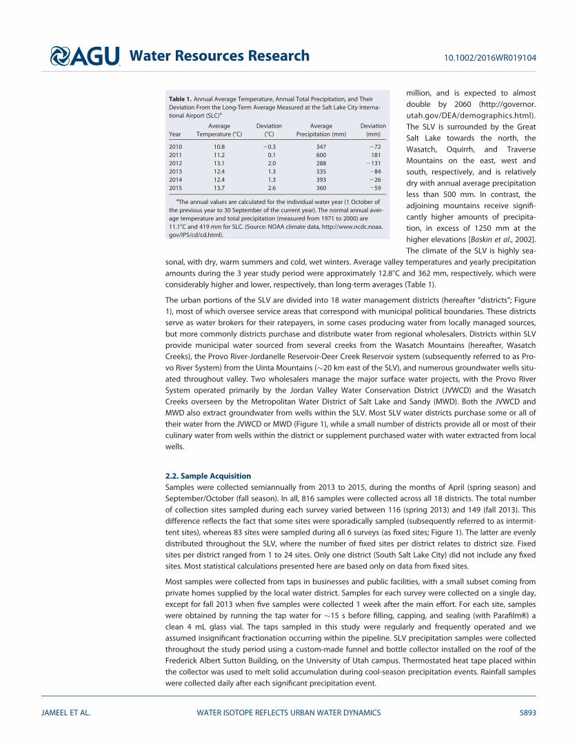
sonal, with dry, warm summers and cold, wet winters. Average valley temperatures and yearly precipitationamounts during the 3 year study period were approximately 12.88C and 362 mm, respectively, which wereconsiderably higher and lower, respectively, than long-term averages (Table 1).

The urban portions of the SLV are divided into 18 water management districts (hereafter ‘‘districts’’; Figure1), most of which oversee service areas that correspond with municipal political boundaries. These districtsserve as water brokers for their ratepayers, in some cases producing water from locally managed sources,but more commonly districts purchase and distribute water from regional wholesalers. Districts within SLVprovide municipal water sourced from several creeks from the Wasatch Mountains (hereafter, WasatchCreeks), the Provo River-Jordanelle Reservoir-Deer Creek Reservoir system (subsequently referred to as Pro-vo River System) from the Uinta Mountains (�20 km east of the SLV), and numerous groundwater wells situ-ated throughout valley. Two wholesalers manage the major surface water projects, with the Provo RiverSystem operated primarily by the Jordan Valley Water Conservation District (JVWCD) and the WasatchCreeks overseen by the Metropolitan Water District of Salt Lake and Sandy (MWD). Both the JVWCD andMWD also extract groundwater from wells within the SLV. Most SLV water districts purchase some or all oftheir water from the JVWCD or MWD (Figure 1), while a small number of districts provide all or most of theirculinary water from wells within the district or supplement purchased water with water extracted from localwells.

2.2. Sample AcquisitionSamples were collected semiannually from 2013 to 2015, during the months of April (spring season) andSeptember/October (fall season). In all, 816 samples were collected across all 18 districts. The total numberof collection sites sampled during each survey varied between 116 (spring 2013) and 149 (fall 2013). Thisdifference reflects the fact that some sites were sporadically sampled (subsequently referred to as intermit-tent sites), whereas 83 sites were sampled during all 6 surveys (as fixed sites; Figure 1). The latter are evenlydistributed throughout the SLV, where the number of fixed sites per district relates to district size. Fixedsites per district ranged from 1 to 24 sites. Only one district (South Salt Lake City) did not include any fixedsites. Most statistical calculations presented here are based only on data from fixed sites.

Most samples were collected from taps in businesses and public facilities, with a small subset coming fromprivate homes supplied by the local water district. Samples for each survey were collected on a single day,except for fall 2013 when five samples were collected 1 week after the main effort. For each site, sampleswere obtained by running the tap water for �15 s before filling, capping, and sealing (with ParafilmVR ) aclean 4 mL glass vial. The taps sampled in this study were regularly and frequently operated and weassumed insignificant fractionation occurring within the pipeline. SLV precipitation samples were collectedthroughout the study period using a custom-made funnel and bottle collector installed on the roof of theFrederick Albert Sutton Building, on the University of Utah campus. Thermostated heat tape placed withinthe collector was used to melt solid accumulation during cool-season precipitation events. Rainfall sampleswere collected daily after each significant precipitation event.

Table 1. Annual Average Temperature, Annual Total Precipitation, and TheirDeviation From the Long-Term Average Measured at the Salt Lake City Interna-tional Airport (SLC)a

YearAverage

Temperature (8C)Deviation

(8C)Average

Precipitation (mm)Deviation

(mm)

2010 10.8 20.3 347 2722011 11.2 0.1 600 1812012 13.1 2.0 288 21312013 12.4 1.3 335 2842014 12.4 1.3 393 2262015 13.7 2.6 360 259

aThe annual values are calculated for the individual water year (1 October ofthe previous year to 30 September of the current year). The normal annual aver-age temperature and total precipitation (measured from 1971 to 2000) are11.18C and 419 mm for SLC. (Source: NOAA climate data, http://www.ncdc.noaa.gov/IPS/cd/cd.html).



http://governor.utah.gov/DEA/demographics.html


http://www.ncdc.no

The semiannual survey, in hydrologically contrasting seasons, was designed to capture potential seasonaldifferences in the tap water isotopes. As the largest isotopic differences in environmental water in the SLVhave been previously observed during the spring and fall seasons [Bowen et al., 2007a], we opted for thoseperiods. A similar strategy has previously been used in studying tap water isotope ratios across the UnitedStates, where sampling efforts were conducted in the months of February and August to capture seasonaldifferences in tap water isotopes [Landwehr et al., 2014].

2.3. Isotope AnalysisPrior to analysis, the samples were stored at 48C in a refrigerator. The isotope ratios of samples were ana-lyzed within a few weeks of their collection at the Stable Isotope Ratios for Environmental Research (SIRFER)facility, University of Utah, on a Cavity Ring-Down Spectroscopy (CRDS; Picarro L2130-i, Santa Clara, CA) ana-lyzer. All the sample values are reported using d notation, where d5Rsample/Rstandard 2 1, R5 2H/1H or18O/16O, and the VSMOW water standard is referenced. Four injections of each sample were measured andcorrected for memory effects and through-run drift, and calibrated to the VSMOW-SLAP scale, using a suiteof three laboratory reference waters (PZ: 16.9&, 1.65&; PT: 245.6&, 27.23&; UT: 2123.1&, 216.52&; ford2H and d18O, respectively). Details of the calibration and correction procedure are reported in Geldern and

Figure 1. Tap water sampling sites within the 18 water districts of the SLV metropolitan area. The blue and yellow regions show areas serviced by MWD and JVWCD, respectively,throughout the study period; since 2015 the Riverton water district has been serviced by JVWCD.



Barth [2012] and Good et al. [2014b]. Accuracy and precision were checked throughout the period of analy-sis using laboratory reference waters; the analytical precision of the instruments used was within 6

0.20& and 6 0.04& for the hydrogen and oxygen isotopes based on the standard deviation of themean calibrated PT values from runs conducted during the analysis period (April 2013 to October2015).

2.4. Spatiotemporal AnalysisWe analyzed data from fixed sites to identify those sites with common isotopic characteristics throughoutthe sampling period. Principal Component Analysis (PCA) was performed on the data set to remove the cor-relation among the variables. The analysis used k-means clustering, which splits the data set into k groupsby maximizing between-group variation relative to within-group variation. Clustering was based on d2H,d18O and deuterium excess (d 5 d2H – 8 3 d18O) values from all six surveys, and the groups were obtainedusing the Hartigan-Wong algorithm in R 3.2.2 [R Core Team, 2015].

Given the common modes of isotopic variation exhibited by sites within each cluster group, we evaluated thepossibility that information on the isotope ratios and distribution of waters from each group could be used to pre-dict the values that would be observed at ‘‘unsampled’’ locations within the SLV. For each cluster group (c) and

each survey (s), we calculated the mean isotopic value �dc;s� �

. We then estimated the average tap water isotope

value for each water district (wd) and each survey (s), defined as a weighted average of the mean values for each

Table 2. Summary Statistics for the Stable Oxygen and Hydrogen Isotopic Composition and Deuterium Excess (d) for Samples Collectedin the Salt Lake City Metropolitan Area From Spring 2013 to Fall 2015a

All Sites Fixed Sites

Season n d18O d2H d n d18O d2H d

Average 215.9 2119.9 7.1 215.9 2119.8 7.0SD 1.1 5.7 3.2 1.1 6.0 3.4

Spring 2013 Minimum 116 217.5 2131.9 26.0 83 217.5 2131.9 26.0Maximum 211.5 297.2 11.2 211.5 297.2 11.2Range 6.0 34.7 17.2 6.0 34.7 17.2

Average 215.6 2119.4 5.6 215.6 2119.2 5.6SD 1.0 5.6 3.0 1.2 6.4 3.5

Fall 2013 Minimum 149 217.2 2128.4 25.5 83 216.9 2125.3 25.5Maximum 211.1 294.3 10.1 211.1 294.3 10.1Range 6.1 34.1 15.6 5.8 31.0 15.6

Average 215.8 2119.1 6.9 215.7 2118.5 6.9SD 1.0 5.5 3.1 1.2 6.4 3.6


Average 215.6 2118.7 6.0 215.5 2118.4 6.0SD 1.0 5.2 3.0 1.2 6.1 3.4


Average 215.6 2117.9 6.5 215.5 2117.6 6.5SD 0.9 4.7 3.2 1.0 5.2 3.6


Average 215.0 2115.8 4.3 215.0 2115.5 4.3SD 0.9 4.7 2.8 1.0 5.3 3.2


aStatistics shown include average, standard deviation (SD), minimum, maximum, range, and number of sites (n). Values of d2H, d18Oand d are expressed in & relative to Vienna Standard Mean Ocean Water (VSMOW).



cluster group represented within the district �dwd;s5P

�dc;sð Þ3nð Þ.P

n

� �, where n is the total number of sites

within a cluster group andP

n is the total number of sites in a water district. We tested these predictions againstindependent data from the intermittent sites, calculating residuals for each intermittent site measurement as the

difference between the observed value and the calculated �dwd;s for a given district and survey.

We compared the mean of the isotope ratios (d2H and d18O, paired t test) for the different surveys and cal-culated the spatial autocorrelation (Moran’s I value) in the isotope ratios for the different surveys. We alsoestimated the mean water isotope ratios �dt;s

� �of the total tap water flux (t) across the SLV for each survey

period. We included all the sites (intermittent and fixed) in calculating �dt;s. We began by calculating the iso-flux �dwd;s;all X Qwd;s

� �for each district and each survey, using yearly water consumption data (Qwd) available

for 2014–2015 from the Utah Division of Water Rights website (water use publications, http://www.water-rights.utah.gov/distinfo/wuse.asp) to estimate district-specific value. The SLV-wide isoflux was calculated asthe sum of the isofluxes of all the districts, and was divided by the total water use across the SLV to obtain

the valley-wide mean tap water isotopic composition �dt;s5P

�dwd;s;allð Þ3Qwd;sð Þ.P

Qwd;sð Þ

� �. All statistical

calculations were performed in R 3.2.2 [R Core Team, 2015] and maps were plotted using ArcGIS 10.2 (ESRI;Redlands, CA). Last, we explored possible correlations with data obtained from the United States CensusBureau, including population and median household income, which we aggregated for each municipaldistrict and water district.

Figure 2. Isotopic composition of the tap water samples across the SLV metropolitan area. The black and the blue-dashed lines representthe global meteoric water line (d2H 5 8 3 d18O 1 10) and the local meteoric water line (d2H 5 7.45 3 d18O 2 1.66), respectively. The redlines and equation represent ordinary least squares best fits to data from each survey. (a) spring 2013, (b) fall 2013, (c) spring 2014, (d) fall2014, (e) spring 2015, and (f) fall 2015.



http://www.waterrights.utah.gov/distinfo/wuse.asp


3. Results

Across all surveys, the stable isotope ratios of SLV tap waters ranged from 2131.9 to 295.2& for d2H(average 5 2118.0&, SD 5 5.0&) and from 217.5 to 211.1& for d18O (average 5 215.6&, SD 5 1.0&).The distribution of d values is similar for all the surveys across the three years, and is nonnormal, multimod-al, and positively skewed for both elements. A majority of the tap water data from the first five surveyswere situated within 2& (for d2H) of the Local Meteoric Water Line, as defined by precipitation data col-lected during the 2013–2015 period (LMWL, d2H 5 7.45 3 d18O 2 1.7, R2 5 0.98), with a small subset ofsamples (16%) falling well below the LMWL (Figure 2). For fall 2015 survey, a larger fraction of the sam-ples (63%) fell at least 2& below the LMWL (Figure 2). Deuterium excess values, which decrease asevaporative losses from soils and surface waters increase, ranged from 10.9 to 25.5& (average 5 6.4&).We fit a local evaporation line (LEL) to the data from each survey and found that slopes for all surveyswere similar and between 4.9 and 5.3. These slopes are comparable to that of the LEL (slope 5 5.2)observed for evaporating surface waters collected in the region [Nielson and Bowen, 2010].

The unweighted average d2H and d18O values for the entire SLV (fixed and intermittent sites combined)varied between the different survey periods (Table 2). Overall, we noted a positive trend in the isotoperatios during the survey period, with average values for the SLV increasing by more than 4 and 0.9& ford2H and d18O. The SLV tap water samples showed a large but consistent isotopic range (� 30& and �6&

for d2H and d18O) for all the different surveys. Intradistrict isotopic ranges were smaller and were also sim-ilar among the different surveys, with the average intradistrict range (for districts with> 5 sites) varyingbetween 1.0 and 3.0& for d2H and between 0.2 and 0.5& for d18O. Statistical tests based on data fromfixed sites only support these patterns. Differences in the average d2H and d18O values between most ofthe different surveys were statistically significant (paired t test for means, p< 0.05, Table 3). No significantdifferences in the variance for d2H, d18O and d were detected across the different surveys (F test for vari-ance, p> 0.05).

Tap water d18O values exhibited weak spatial autocorrelation for all surveys (Moran’s I value forspring 2013 through fall 2015 5 0.14, 0.24, 0.24, 0.17, 0.21, and 0.27, Z 5 4.5, 6.5, 7.7, 6.5, 6.4, and 8.4,for all p< 0.05). Similar spatial correlation was observed for d2H and d. Samples collected on the east-ern side of the SLV tended to have slightly lower d2H and d18O values compared to those collectedon the western side (Figure 3). The highest isotopic values (> 2100& and>212& for d2H andd18O) were consistently observed on the northwestern side of the valley and the lowest values foreach sampling event were observed on the eastern side of the valley (< 2120& and<216& ford2H and d18O). In general, sites situated close to each other (ground distance< 0.2 km) and fallingwithin the same water district tended to have similar isotopic ratios, but adjacent sites straddlingboundaries between some (but not all) water districts showed substantial differences (Figure 3).Large differences at closely situated sites were infrequent, but were consistently observed between

Table 3. Results of Paired t-Tests for Isotopic Data From the Surveysa

d18O d2H

Mean of the Differences p-Value Mean of the Differences p-Value

Spring 2013 to Fall 2013 20.24 <0.05 20.54 0.13Spring 2013 to Spring 2014 20.18 <0.05 21.31 <0.05Spring 2013 to Fall 2014 20.31 <0.05 21.37 <0.05Spring 2013 to Spring 2015 20.32 <0.05 22.11 <0.05Spring 2013 to Fall 2015 20.87 <0.05 24.27 <0.05Fall 2013 to Spring 2014 0.06 0.21 20.75 <0.05Fall 2013 to Fall 2014 20.05 0.25 20.82 <0.05Fall 2013 to Spring 2015 20.07 0.22 21.56 <0.05Fall 2013 to Fall 2015 20.62 <0.05 23.72 <0.05Spring 2014 to Fall 2014 20.11 <0.05 20.07 0.78Spring 2014 to Spring 2015 20.14 <0.05 20.81 <0.05Spring 2014 to Fall 2015 20.68 <0.05 22.97 <0.05Fall 2014 to Spring 2015 0.02 0.62 20.73 <0.05Fall 2014 to Fall 2015 20.57 <0.05 22.89 <0.05Spring 2015 to Fall 2015 20.54 <0.05 22.15 <0.05

aValues of d2H and d18O are expressed in & relative to Vienna Standard Mean Ocean Water (VSMOW).



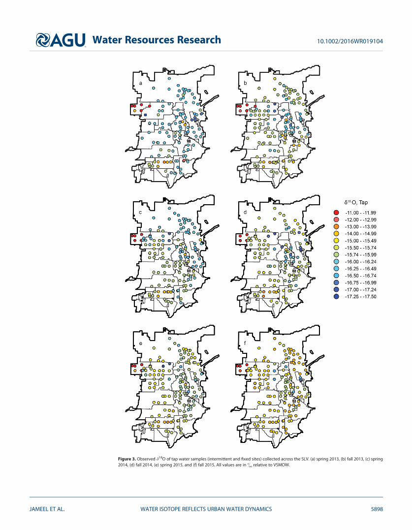
Figure 3. Observed d18O of tap water samples (intermittent and fixed sites) collected across the SLV. (a) spring 2013, (b) fall 2013, (c) spring2014, (d) fall 2014, (e) spring 2015, and (f) fall 2015. All values are in & relative to VSMOW.



two sites (sampled within 500 m of each other) straddling the boundary of the Granger-Hunter andMagna water districts. Isotopic differences between these sites were more than 12& and 4&, ford2H and d18O, during all the surveys (Figure 3).

4. Discussion

4.1. SLV Tap Water Cluster Group PatternsK-means clustering divides the fixed sites into six groups, with 27, 24, 22, 4, 4, and 2 sites per group (Figure4a). The majority of the sites (73 out of 83) are assigned to three main groups. With a few exceptions, thegroups exhibit strong spatial clustering within the SLV, indicating that proximal sites tend to be character-ized by similar tap water isotope ratios and patterns of temporal variation (Figure 4a). Sites belonging togroups 1 and 3 are clustered together in the eastern and northeastern parts of the valley (Figure 4a), withgroup 1 sites exhibiting a higher density in the east-central valley and group 3 being more concentrated inthe northern and southern extremes of this region. The other major group, group 2, dominates a swathe ofthe southern and western valley (Figure 4a) with only a handful of sites impinging on the areas dominatedby groups 1 and 3. Groups 4 and 5 are clustered in two small, distinct regions and with the exception ofone site classified with group 5 (discussed below) each of these groups is constrained to and dominates asingle municipal water district. Group 6 constitutes a pair of sites clustered within the group-1-dominatedregion in the eastern side of the valley.

The coincidence of the group 4 and 5 distributions with water district boundaries, as well as the general—ifimperfect—alignment of the boundary between the regions dominated by group 2, and groups 1 and 3with north-south water district boundaries throughout the central valley, suggests that the role of these dis-tricts in brokering and managing water supplies used by their residents is reflected in the spatiotemporaldistribution of tap water isotopes ratios. However, the larger-scale clustering of sites categorized within themajor groups also suggests a higher order of organization within the regional water distribution system.

Figure 4. Spatial distribution of isotope cluster groups (a), their mean isotopic ratios (b-c) and D-Excess (d) for the six surveys. Black lines inFigures 4b–4d represent the consumption-weighted, regional average values for the entire SLV. All values are in & relative to VSMOW.S13: spring 2013, F13: fall 2013, S14: spring 2014, F14: fall 2014, S15: spring 2015, and F15: fall 2015.



Indeed, the distribution of group 2 and group 3 sites approximates the service regions of the two majorregional wholesalers, the JVWCD and MWD, respectively. Specific links between water sources, manage-ment practices, and the tap water isotope ratios will be discussed in subsequent sections, but the spatialassociation of the data with the footprint of management districts and wholesaler service areas itself pro-vides an indication that the isotopic data reflect aspects of the structure of the water distribution system.

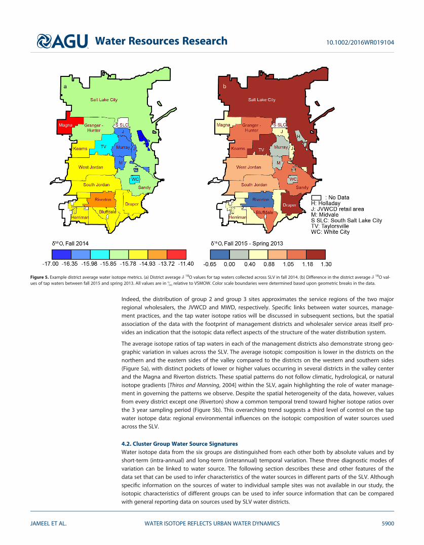
The average isotope ratios of tap waters in each of the management districts also demonstrate strong geo-graphic variation in values across the SLV. The average isotopic composition is lower in the districts on thenorthern and the eastern sides of the valley compared to the districts on the western and southern sides(Figure 5a), with distinct pockets of lower or higher values occurring in several districts in the valley centerand the Magna and Riverton districts. These spatial patterns do not follow climatic, hydrological, or naturalisotope gradients [Thiros and Manning, 2004] within the SLV, again highlighting the role of water manage-ment in governing the patterns we observe. Despite the spatial heterogeneity of the data, however, valuesfrom every district except one (Riverton) show a common temporal trend toward higher isotope ratios overthe 3 year sampling period (Figure 5b). This overarching trend suggests a third level of control on the tapwater isotope data: regional environmental influences on the isotopic composition of water sources usedacross the SLV.

4.2. Cluster Group Water Source SignaturesWater isotope data from the six groups are distinguished from each other both by absolute values and byshort-term (intra-annual) and long-term (interannual) temporal variation. These three diagnostic modes ofvariation can be linked to water source. The following section describes these and other features of thedata set that can be used to infer characteristics of the water sources in different parts of the SLV. Althoughspecific information on the sources of water to individual sample sites was not available in our study, theisotopic characteristics of different groups can be used to infer source information that can be comparedwith general reporting data on sources used by SLV water districts.

Figure 5. Example district average water isotope metrics. (a) District average d 18O values for tap waters collected across SLV in fall 2014. (b) Difference in the district average d 18O val-ues of tap waters between fall 2015 and spring 2013. All values are in & relative to VSMOW. Color scale boundaries were determined based upon geometric breaks in the data.



4.2.1. Low-Variance GroupsGroups 1 and 4 are distinguished by their relatively invariant values across the 3 year sampling period (1standard deviation for group mean d18O values <0.15&, average fall-spring d18O difference <0.1&; Table4; Figures 4b–4d). Although it is possible that multiple isotopically distinct or varying sources were used tosupply the sites constituting these groups, and that the source blend changed in a way that maintained aconstant tap water composition, a more parsimonious explanation is that water was supplied to these sitesfrom an isotopically invariant source. Unlike surface water resources, which are affected by strong seasonalvariation in precipitation water isotope ratios and runoff sources, isotopic values for groundwaters tend toexhibit limited seasonal and highly damped long-term variability [Clark and Fritz, 1997; Wassenaar et al.,2009]. We thus interpret the data from groups 1 and 4 as indicative of groundwater-dominated supplyregions. Isotopic values observed in group 1 are similar to those measured for regional deep groundwatersin the aquifers underlying the eastern part of the valley [Thiros, 2003; Thiros and Manning, 2004], and report-ing data from the water districts supports our interpretation that wells tapping these aquifers constitute alarge part of the water supply to this area (http://www.murray.utah.gov/DocumentCenter/Home/View/1313,http://www.midvalecity.org/dp.aspx?p565). Indeed, tritium and helium-3 dating suggests the mean age ofgroundwater within the SLV to be approximately 15 years, indicating a relatively long-residence time consis-tent with the lack of preservation of seasonal d2H and d18O trends observed in our surveys [Thiros, 2003]. Val-ues for group 4 samples, in contrast, are the highest observed in our data set, and the high isotope ratios andlow D-excess values for these samples are consistent with groundwater recharged at least in part by sourcesthat had experienced substantial evaporation. The values we measured from taps in this area are consistentwith those previously reported for public supply wells constituting the primary water source for the MagnaWater District [Thiros and Manning, 2004]. Measurements for these wells and for other subsurface waters sam-pled in this part of the SLV show high sodium and chloride ion concentrations [Thiros and Manning, 2004],consist with our inference of a distinct, evapoconcentrated recharge source.4.2.2. Seasonal GroupsIsotope data from groups 2 and 3 exhibit variability characterized by seasonal oscillation superimposed ona trend of increasing d2H and d18O through the study period (Figure 4). Overall variance in the mean valuesof groups 2 and 3 is larger than in groups 1 and 4. For both groups (2 and 3), H and O isotope ratios for thefall sampling periods are higher and d values lower, than for the corresponding spring periods (Table 4).This seasonal pattern is stronger for group 3 sites than for group 2. Within group 2, the data are arrayedalong a line in d2H/d18O space that lies below the local meteoric water line (Figure 6b) and within group 3the data show large seasonal variability with values lying above the LMWL in spring and lying on or belowthe LMWL in fall (Table 4, Figure 6c). These tap water lines exhibit slopes of 5.4 and 4.3 for groups 2 and 3,respectively, which are similar to previously observed surface water evaporation line slopes in the region[Kendall and Coplen, 2001; Dutton et al., 2005; Nielson and Bowen, 2010] and suggest that variation in evapo-rative water loss drives much of the isotopic variation observed in tap water from these groups.

As groundwaters are isolated from seasonal evaporation, we interpret groups 2 and 3 to represent tapwaters sourced primarily from one of the two surface water sources employed in SLV. Water productiondata indicates that approximately 60% of water used in the SLV is extracted from surface waters (water usepublications, http://www.waterrights.utah.gov/distinfo/wuse.asp). Further, the districts supplying waters tothe areas with sites in group 2 and 3 are the known service areas of districts supplying water from theJVWCD and MWD, respectively. Comparison of the isotopic characteristics of group 2 and 3 waters suggests

Table 4. Average, Standard Deviation, and Average Difference Between Spring and Fall Isotope Ratios for Different Cluster Groups With-in the SLV Across the Entire Study Perioda

Average Standard Deviation Average Fall to Spring

Group d18O d2H d d18O d2H d d18O d2H d

1 216.2 2121.2 8.5 0.2 0.8 0.5 0.1 0.0 20.62 215.7 2119.7 5.6 0.4 2.0 1.0 0.3 1.6 20.93 215.8 2119.0 7.1 0.5 2.3 2.1 0.6 1.4 23.44 211.3 296.0 25.4 0.1 1.1 0.4 0.1 0.5 20.35 213.9 2110.1 1.4 0.5 2.7 1.1 0.4 2.2 21.16 215.4 2116.8 6.7 0.8 4.6 2.0 21.2 26.6 2.7

aValues of d2H, d18O and d are expressed in & relative to Vienna Standard Mean Ocean Water (VSMOW).



http://www.murray.utah.gov/DocumentCenter/Home/View/

http://www.midvalecity.org/dp.aspx?p=65

http://www.midvalecity.org/dp.aspx?p=65


that the data may document nuancesreflecting differences in these twomajor surface water systems. The low-er variability and incredibly tight cor-relation of group 2 water values alongan apparent evaporation line (Figure6b) is consistent with waters fromthese sites being derived dominantlyfrom a single surface water systemhaving a relatively large storagecapacity and long turnover time.Extraction from the Provo River sys-tem constitutes the majority (65%) ofthe water supplied by JVWCD (2014Annual report, https://jvwcd.org/pub-lic/highlights). Although we were notable to estimate a system-wide turn-over time, the Provo River systemincludes two large (capacity: 448 3

106 m3 and 188 3 106 m3) andnumerous small reservoirs, harvestswater from a large catchment area(�1500 km3), and is operated as amajor source year-round.

In contrast, the greater variability ofthe group 3 data about their evapora-tion line (Figure 6c) suggest derivationfrom a more isotopically ‘‘volatile’’source and/or more dynamic use ofmultiple water sources to supply tapsin this group. Indeed, the smaller stor-age capacity of the multiple Wasatchcreek systems managed by MWDshould translate into lower transittimes and greater isotopic variabilityof these sources. The seasonal natureof runoff from Wasatch creek [Bardsleyet al., 2013] watersheds mean that

MWD and their client districts supplement water from these sources with water from the Provo River systemduring low-flow seasons (http://www.mwdsls.org/pdfs/Annual_Report_2014_ Final.pdf). We note that isotopicvalues of group 2 and 3 sites converge, in general, during the fall sampling events, consistent with a conver-gence of water sources across the region during the fall low-flow period.4.2.3. High Variance GroupsGroups 5 and 6 are characterized by substantial isotopic variation over the study period, but exhibit tempo-ral patterns of variation that are distinct from those of the ‘‘seasonal’’ groups. In addition, data from thesesmall groups have much higher within-group variance than seen for groups 1–4 (e.g., for d18O the averagewithin-group standard deviation for a given sampling period is 0.94 and 0.75& for groups 5 and 6, respec-tively, and <0.38& for all other groups). Isotopic data for sites within each of the high variance groupsexhibit some common features, but do not follow a single, uniform trend (Figure 7).

Sites within cluster group 5 show two distinct patterns of variation that map onto the geographic distribu-tion of these sites. Tap water isotope ratios for three sites within the Riverton water district are relatively sta-ble or decline slightly over the first 2 years of sampling and then drop by �1& over the final year ofsampling (Figure 7a). During the final sampling event (fall, 2015), the values at these sites are

Figure 6. Evaporative trends in SLV tap waters across the 3 year sampling period.Values shown are consumption-weighted SLV-wide means (a) and mean values forcluster groups 2 (b) and 3(c). The blue-dashed line in each plot is the LMWL and thered line is the best fit line to the data, representative of the local evaporation line(LEL). Filled black circles in Figures 6a and 6b show inferred preevaporation sourcewater isotopic compositions estimated by the intersection of the LEL and LMWL.



http://https://jvwcd.org/public/highlights

http://https://jvwcd.org/public/highlights

http://www.mwdsls.org/pdfs/Annual_Report_2014_Final.pdf

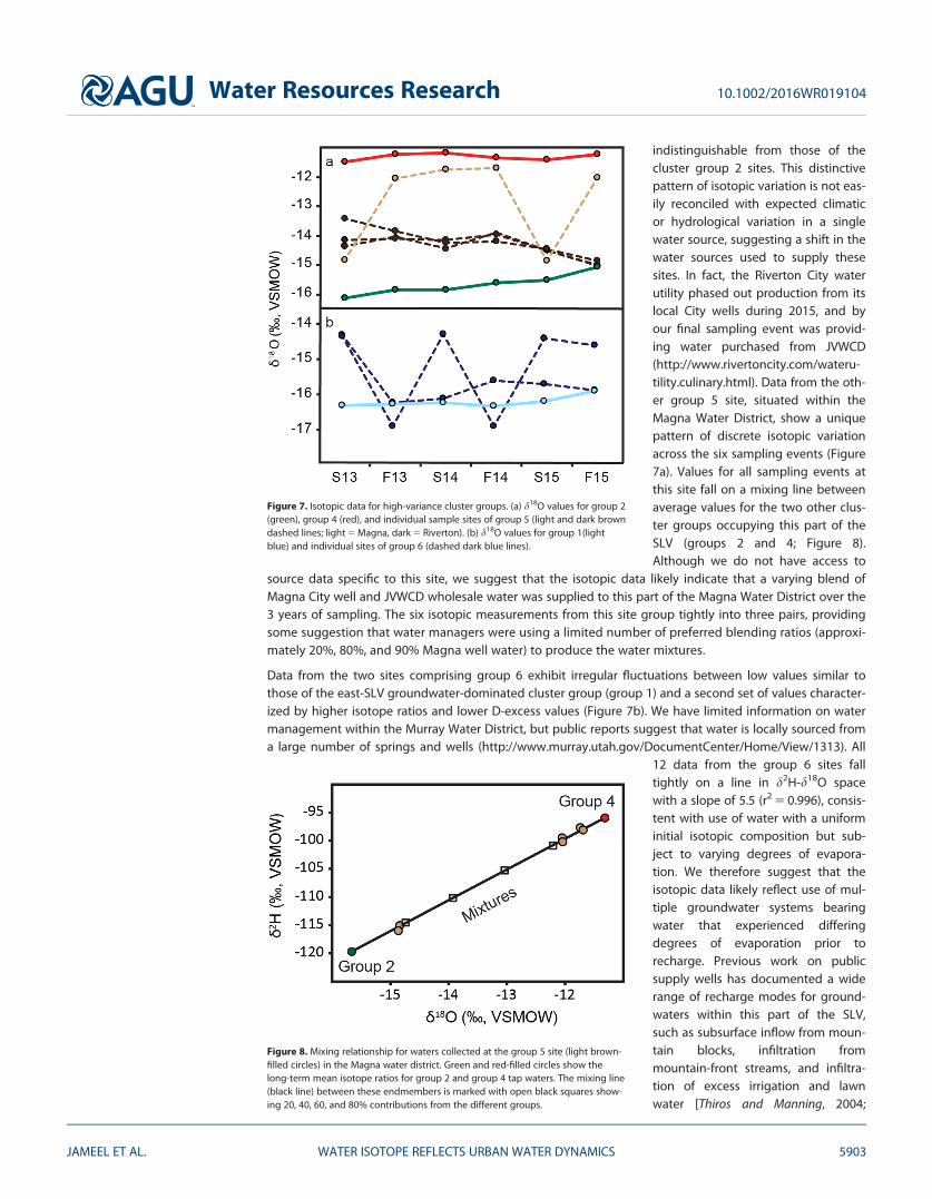
indistinguishable from those of thecluster group 2 sites. This distinctivepattern of isotopic variation is not eas-ily reconciled with expected climaticor hydrological variation in a singlewater source, suggesting a shift in thewater sources used to supply thesesites. In fact, the Riverton City waterutility phased out production from itslocal City wells during 2015, and byour final sampling event was provid-ing water purchased from JVWCD(http://www.rivertoncity.com/wateru-tility.culinary.html). Data from the oth-er group 5 site, situated within theMagna Water District, show a uniquepattern of discrete isotopic variationacross the six sampling events (Figure7a). Values for all sampling events atthis site fall on a mixing line betweenaverage values for the two other clus-ter groups occupying this part of theSLV (groups 2 and 4; Figure 8).Although we do not have access to

source data specific to this site, we suggest that the isotopic data likely indicate that a varying blend ofMagna City well and JVWCD wholesale water was supplied to this part of the Magna Water District over the3 years of sampling. The six isotopic measurements from this site group tightly into three pairs, providingsome suggestion that water managers were using a limited number of preferred blending ratios (approxi-mately 20%, 80%, and 90% Magna well water) to produce the water mixtures.

Data from the two sites comprising group 6 exhibit irregular fluctuations between low values similar tothose of the east-SLV groundwater-dominated cluster group (group 1) and a second set of values character-ized by higher isotope ratios and lower D-excess values (Figure 7b). We have limited information on watermanagement within the Murray Water District, but public reports suggest that water is locally sourced froma large number of springs and wells (http://www.murray.utah.gov/DocumentCenter/Home/View/1313). All

12 data from the group 6 sites falltightly on a line in d2H-d18O spacewith a slope of 5.5 (r2 5 0.996), consis-tent with use of water with a uniforminitial isotopic composition but sub-ject to varying degrees of evapora-tion. We therefore suggest that theisotopic data likely reflect use of mul-tiple groundwater systems bearingwater that experienced differingdegrees of evaporation prior torecharge. Previous work on publicsupply wells has documented a widerange of recharge modes for ground-waters within this part of the SLV,such as subsurface inflow from moun-tain blocks, infiltration frommountain-front streams, and infiltra-tion of excess irrigation and lawnwater [Thiros and Manning, 2004;

Figure 8. Mixing relationship for waters collected at the group 5 site (light brown-filled circles) in the Magna water district. Green and red-filled circles show thelong-term mean isotope ratios for group 2 and group 4 tap waters. The mixing line(black line) between these endmembers is marked with open black squares show-ing 20, 40, 60, and 80% contributions from the different groups.

Figure 7. Isotopic data for high-variance cluster groups. (a) d18O values for group 2(green), group 4 (red), and individual sample sites of group 5 (light and dark browndashed lines; light 5 Magna, dark 5 Riverton). (b) d18O values for group 1(lightblue) and individual sites of group 6 (dashed dark blue lines).



http://www.rivertoncity.com/waterutility.culinary.html

http://www.rivertoncity.com/waterutility.culinary.html

http://www.murray.utah.gov/DocumentCenter/Home/View/

Bexfield et al., 2011], but not the wide range of isotopic compositions measured here for group 6 tap waters.

The ability to distinguish and map the structure of the water distribution system with water isotopes, and toestablish connections between taps and climatic water sources, could support numerous applications. Inareas with diverse water sources and complex networks of public and private stakeholders, the tools devel-oped here could support monitoring and enforcement of water rights. Information connecting water sam-pled within distribution systems or at the point of use to environmental sources could be valuable inevaluating the susceptibility of these waters to climatic changes or water quality impairment (e.g., as exem-plified by the contrasting susceptibilities of water from surface or fossil groundwater sources). In addition,information on connectivity within distribution systems could be of use in tracking of contaminants andnonconservative tracers introduced within the system itself and response to critical water contaminationevents.

4.3. Long-Term Isotopic TrendThe waters available to the growing population of SLV are sensitive to seasonal climate dynamics. The2013–2015 period featured above average temperatures and below average precipitation across the SLVand adjacent watershed areas, with the last above-average water year occurring during 2011 (Table 1).These factors should significantly affect the d2H and d18O values of SLV tap waters. Our estimate of the SLV-wide water isotope budget gives mean tap water isotope ratios of 2121.3& and 216.1& (d2H and d18O) inspring 2013 and suggests a nearly monotonic increase for d2H and an increasing trend with a superimposedseasonal oscillation for d18O during the subsequent samplings (Figures 4b and 4c). The overall increase inmean tap water isotope ratios is more than 5& and 1& for d2H and d18O, respectively, between 2013 and2015. Average values for the individual surveys lie along a line of slope 5.0 (r2 5 0.92), suggesting that theevolution in basin-wide tap water isotope ratios over the course of the study period may reflect trendtoward increasing evaporative water loss with time. We suggest that the combination of below-averagerecharge of reservoirs and above-average evaporative demand may have driven a progressive increase inevapoconcentration of surface water resources supplying the SLV. Based upon our data, it is difficult to con-strain weather the isotopic enrichment is due to elevated temperature and/or due to below average precip-itation in the region.

To understand the impacts of these climate dynamics on SLV water supply, we estimate the total evapora-tive loss from watersheds, reservoirs, and distribution systems employed by districts in SLV using the modi-fied Craig-Gordon (C-G) model [Craig and Gordon, 1965; Skrzypek et al., 2015]. The model requires initial andpostevaporation values of the stable isotope composition of the water pool and estimated values for thestable isotope composition of moisture in the ambient atmosphere, atmospheric temperature, and humidi-ty. For our analysis, the initial source water value was estimated by projecting the evaporation line definedby the consumption-weighted average tap water isotope data back to the SLV LMWL (2120.6& and216.0& for d2H and d18O, respectively, Figure 6a). The isotopic composition of the ambient air moisturewas estimated using the methods described in [Gat, 1995], [Gibson and Reid, 2014], and [Gibson et al., 2016].We used mean annual temperature and humidity values from Salt Lake International Airport (http://www.ncdc.noaa.gov/IPS/cd/cd.html; T 5 12.4, 12.4 and 13.78C, RH 5 0.52, 0.51, and 0.51 in 2013, 2014, and 2015,respectively), which were intended to provide only a rough approximation of the conditions within the SLVwater source region during warm-season periods when the majority of evaporation occurs [Gibson et al.,2008, 2016]. We used the kinetic fractionation factors appropriate for open-water evaporation in a continen-tal environment [Vogt, 1976]. Although some fraction of the evaporation recorded in the tap water datamay have occurred within soils of the SLV water supply watersheds, recent studies suggest that soil evapo-ration has a limited effect on the isotopic composition of groundwaters and streams [Evaristo et al., 2015;Good et al., 2015]. Our calculation suggests that evaporative losses from the SLV water supply increasedfrom 1 to 1.5% of the total water flux in 2013 to 4 to 6% in 2015. Using yearly water consumption data forthe SLV obtained from the Utah Division of Water Rights website (see section 2.4), these values translateinto >15,000 m3 of evaporative loss per day in 2015 (assuming a conservative loss rate of 4%). Thisenhanced loss to the atmosphere would equate to $2.25 million of revenue loss in 2015 (calculated at cur-rent rates of $1.16 per unit within Salt Lake City; 1 unit 5 2.83 m3) if translated into reduced extractions, orsignificant ecological impacts if extraction remained unchanged.



http://www.ncdc.noaa.gov/IPS/cd/cd.html

http://www.ncdc.noaa.gov/IPS/cd/cd.html

The evapoconcentration trendobserved within the SLV-wide, con-sumption-weighted data is even morestrongly expressed in data from clus-ter group 2, which is interpreted toprimarily record values from the high-ly impounded Provo River System. C-G calculations for data from thisgroup, using meteorological valuesestimated from measurements atDeer Creek Reservoir (T 5 6.5, 8.0, and8.48C in 2013, 2014, and 2015;RH 5 0.50 for all years), suggest evap-orative losses of 2–2.5%, 3.5–5%, and5.5–8% in 2013, 2014, and 2015. TheProvo system has a multiyear turnovertime (at least 1.3 years, estimated con-sidering only the ratio of Provo Riverinflow to the capacity of the twomajor reservoirs within the system),and the enhanced accumulation ofevaporative influence over the multi-year climatic anomaly of the study isnot surprising in this context.

Although the calculations presentedhere are simple first-order estimates,and could be refined with the collec-tion of additional field data to betterconstrain model parameters, theyindicate the potential to reconstructdynamic changes in evaporativewater loss from large-scale water sup-ply systems and quantify these losses

as a component of the water budget of a major metropolitan region. The data suggest that during a 3 yearperiod of drier and warmer than average climate these losses accelerated and accumulated, removing anadditional 9400 m3 to 11400 m3 of water per day from the SLV public supply system at the end of 2015 rela-tive to the beginning of the study period.

4.4. Demographic AssociationsBecause the water supply system of the SLV has been developed over time to provide reliable water distri-bution to a dispersed and evolving population, we anticipate that the isotope data, reflective of the sourcesof water used, may reveal different patterns and strategies of water supply management that correlate withvariation in demographic characteristics of SLV communities. We observe significant positive correlationbetween the range of isotope ratios for all tap water samples collected in a given water district (calculatedas the difference between maximum and minimum isotope ratios observed in the district over the entiresampling period) and the population of that district (Figure 9a). The largest isotopic ranges occur inGranger-Hunter and Salt Lake City, the two districts with the highest population. Low ranges are observedfor smaller districts such as Midvale, Holladay, and Bluffdale. Given the association between water sourcetype and isotope values introduced in section 4.2, this correlation may reflect the tendency for larger dis-tricts to use water from multiple sources to meet their higher water demands. Similar relationships havebeen reported on a national scale: 70% of hydrological basins with population less than 100,000 inhabitantsrely only on single source of water, whereas basins with large population, particularly in water-limitedregions such as the southwestern United States, commonly rely on multiple sources and nonlocal water[Fort et al., 2012; Landwehr et al., 2014]. A recent isotope-based analysis of water use across the western

Figure 9. Comparison of tap water isotope metrics with select socioeconomicdata. (a) Correlation between water district population and the range of observedd18O values (Magna and Murray districts not included). (b) Correlation between dis-trict average per household annual income and average tap water D-Excess value(Magna not included). Red, blue, and grey circles represent fall 2013, fall 2014, andfall 2015, respectively. Regression line includes data from all the 3 years. All regres-sions are statistically significant (p< 0.05).



United States has shown population to be a significant predictor of nonlocal water use [Good et al., 2014a].The reliance of districts with large population on multiple sources of water has implications for the resil-ience of these districts under situations of water scarcity. Importing water from an external source can bebeneficial under scenarios of local water shortage; however, it may increase exposure to regional or extralo-cal drought.

Initial development of the SLV occurred at the northeastern edge of the basing along the base of theWasatch Mountains in and around Salt Lake City (SLC). Later development led to westward and southwardexpansion of the urbanized area. Historic rights to water from the Wasatch creeks are allocated to manystakeholders within the SLV, but center on the cities of SLC and Sandy. Some cities with a later urbanizationhistory, such as Midvale and Murray, used groundwater to cater its population. With the increase in thedemand for water due to increasing population, the Provo River system was developed and used to sourcewater for most of the cities in the south and west of the valley.

We observe a weak yet significant negative correlation between average income of SLV municipal districtsand the average D-excess values of fall season tap water (Figure 9b). This relationship is not apparent duringthe spring season. Given the association of low fall-season deuterium excess values with surface water evap-oration, as noted above, we hypothesize that the observed relationship indicates greater surface water con-sumption in districts with higher per-household income. This may reflect the geographic and historicstructure of the urban area, as described above, where many of the affluent areas are situated in closerproximity to mountain surface sources and within areas of earlier development that often retain historicallocations of surface water rights. Another possible explanation may be the selective use of higher-qualitysurface waters by water managers in more affluent districts or the relative preference of wealthier commu-nity to develop in regions catered by surface waters. Given that majority of the SLV groundwater wells arelocated in and around the basin center, we consider the former, circumstantial possibility to be more likely.

4.5. Implications: Future Water ManagementThe population of the SLV is anticipated to double over the next 40 years (http://governor.utah.gov/DEA/demographics.html), and the resultant demands on water resources promise to be a significant challengeto sustainable development of this semiarid basin. Our isotopic assessment highlights several aspects of themunicipal water systems supplying the SLV that are germane to planning for and understanding thesefuture water resource challenges. First, our calculations show significant increase in evaporative losses with-in the system over the 3 year sampling period, likely attributable to the atypically warm and dry weatherthat persisted throughout the study. Given that majority of municipal water used within the SLV is currentlysourced from surface water and the proposed development of water resources to satisfy future demandsassociated with population growth focuses primarily on surface water systems of the Central Utah Projectand Bear River, SLV communities are and will continue to have strong exposure to changes in evaporativelosses from these systems. Studies have projected a mean annual temperature increase of 1–38C in theregion by the mid-21st century, with stronger summer warming than winter [Jardine et al., 2013], and ourdata suggest that evaporative losses from existing SLV surface water supplies approaching 10% under theseconditions could be plausible. Moreover, the isotopic data clearly show that short-term (year-to-year) climat-ic variability can have a significant impact on evaporative loss from water resources, detectable even at thescale of the entire SLV metro area. Historically, water managers have done a poor job incorporating theimpacts of climatic variability in water resource planning [Craig, 2010], but as the gap between supply anddemand narrows in this and other water-scarce regions, a greater recognition of variability, both in terms ofinputs to hydrologic systems but also evaporative losses, will become increasingly important.

In addition, our data suggest that different parts of the SLV metro area may have different levels of expo-sure to future climatic variability and long-term change. Evaporative trends were weak or not detectable forsites within cluster groups 1 and 4, reflecting the damping of climatic variability by the groundwater sys-tems supplying these sites. Although these sources may be more stable to fluctuations in hydroclimate,greatly increased extraction of groundwater in the SLV is unlikely to be sustainable. Groundwater extractedfrom the western part of the valley is of low quality and requires treatment, including reverse osmosis andultra violet treatment, to make it fit for human consumption (www.itrcweb.org/miningwaste-guidance/cs48_kennecott_south.htm). Most of the groundwater wells in the valley exhibited an increase in the con-centration of dissolved solids from 1988–1992 to 1998–2002, with some wells on the eastern side displaying





http://www.itrcweb.org/miningwaste-guidance/cs48_kennecott_south.htm

http://www.itrcweb.org/miningwaste-guidance/cs48_kennecott_south.htm

an increase of more than 20%, likely due to lateral inflow of water with high solute concentrations from thewestern parts of the valley [Thiros, 2003]. Further, all the wells with modern water showed presence ofanthropogenic compounds, suggesting human contamination [Thiros, 2003]. The low quality of ground-waters has already led some districts such as Riverton to migrate to surface water sources. Given that dis-tricts currently relying primarily on groundwater supplies are among the least affluent in the SLV, futuredeclines in the stability of regional surface water sources and greater demand for groundwater could havesignificant impacts on local water markets and the balance of water rights ‘‘power’’ within the region.

4.6. City-Scale Tap Water Isotope PredictionsIsotopic signatures from environmental water sources are incorporated in plant and animal tissues [Schoelleret al., 1986] and have been used to study wildlife migration, the geographic origin of foods, drugs andhuman remains, and in forensic analysis [Hobson and Wassenaar, 1996; Hobson et al., 1999; Ehleringer et al.,2008; Chesson et al., 2010; Bartelink et al., 2014]. These applications require knowledge of the geographicdistribution and variation of water source isotope ratios [West et al., 2010; Kennedy et al., 2011], but humanand product-focused applications have generally used regional or national-scale surveys and models of pre-cipitation or tap water to guide interpretation of sample data. As demonstrated here and in a limited num-ber of previous studies [Williams, 1997; Kennedy et al., 2011; Good et al., 2014a; Landwehr et al., 2014], theseregional assessments may not capture the local-scale variations in areas that rely on multiple water sourcesor import nonlocal water, potentially leading to interpretive bias or error or limiting the precision of geolo-cation analyses obtained using the isotopic data. Intensive city-scale sampling campaigns are labor-intensive and costly; however, the development of generalizable approaches to predict urban tap water iso-scapes without onerous data overhead is desirable.

The data from our study provide spatially and temporally resolved documentation of city-scale variation intap water isotope ratios that can be used both to evaluate the potential significance of this variation forforensic applications and to develop and test methods for urban tap water isoscape prediction. The

Figure 10. Predictive SLV tap water map and validation. (a) Estimated average SLV tap water d18O values for the study period based on cluster group isotope values and spatial distribu-tion, as described in the text. (b) District average residuals calculated using data from intermittently sampled sites. All values are in & relative to VSMOW.



observed range and standard deviation (SD) of the isotope ratios in the SLV (intermittent and fixed sitescombined) were greater than 30& and 4.5& for d2H, and 5.7& and 0.9& for d18O, respectively, for eachsampling period. Although these values are consistent with estimates of local variability and predictiveuncertainty derived from large-scale tap water studies [Bowen et al., 2007b; Landwehr et al., 2014], the newdata elucidate important aspects of the structure of this variation that are not apparent in the large-scalestudies. First, the data demonstrate that the majority of the variation within SLV tap water isotope ratios isspatial, rather than temporal, in origin, with most individual sampling sites exhibiting a minor range of val-ues across the 3 year period relative to the range observed among sites. This suggests the potential for resi-dents of subregions of the SLV to assimilate distinctive isotopic signatures from their local water supplies,although further work will be required to assess the degree to which movement of such individuals withinthe region and spatiotemporal averaging will diminish the actual expression of such signatures.

Second, our data document and characterize strong links between the spatial distribution of tap water iso-tope ratios and the water management systems of the SLV, providing a basis for modeling and predictionof local-scale water isotope patterns within the urban area. Most previous isoscape models for tap waterhave relied on natural spatial, climatic, or physiographic variables to predict water isotopic composition, butas our data demonstrate the spatial structure of isotopic variation within urban public supply systems is notnecessarily determined by these variables. Based on our results, we adopt the SLV water management dis-tricts as our spatial map unit and estimate the long-term annual average tap water isotope distributionacross the valley using information on cluster group isotopic values and distribution, as described in Meth-ods. The resulting map (Figure 10a) shows the northeast-southwest trends across the valley which we previ-ously attributed to use of different surface water sources, as well as pockets of distinct, higher, or lowervalues associated with localized groundwater use. As validation of the map, we calculated differencesbetween the predicted water isotope values for each district and the observed values of tap water from theintermittently sampled sites situated within that district. These model residuals are normally distributed,with a standard deviation of 0.3& for d18O and a mean of 0.03&. Large residual values (> 0.5&) occur pri-marily in the Magna and Riverton water districts (Figure 10b), where, as described above, temporal switch-ing between isotopically distinct water sources was observed. For comparison, the standard deviation ofresiduals from these same sites when compared with the predictions of the national-scale model of Bowenet al. [2007b] is 1.0& for d18O, showing that substantial improvement results from incorporating informa-tion on the local water management system.

This analysis suggests the potential to characterize and accurately map the variation in tap water isotoperatios across a large urban center with fragmented and heterogeneous water management systems.Although the map presented here was based on a large number of physical samples, the approach may begeneralized and applied in ways that maximize the predictive value of more limited physical sample data.In our workflow, the isotopic data were used both to identify the spatial structure of the water supply sys-tem and to characterize the isotopic composition of the water associated with different parts of that system(the cluster groups). In many cases, the entire workflow may not be dependent on collection of new sampledata. To the degree that the structure of the SLV water supply system is static, for example, one could uselimited, targeted sampling to characterize isotope ratios of waters associated with the already-defined clus-ter groups and create revised tap water isoscapes for future time periods. It is also possible that in many cit-ies independent information on the structure of the water management system, along with limited sampledata or models characterizing the isotopic composition of source waters, could be used to predict tap waterisotope distributions without spatiotemporally intensive sampling at the point of use. In either case, atten-tion to the potentially dynamic nature of both system structure/management (e.g., as seen for the Rivertonwater district during our study) and source water composition will continue to be warranted, as our datasuggest that both factors drove perceptible changes in SLV tap water isotope ratios during our period ofstudy.

5. Conclusions

Water isotopes have been used extensively to study natural components of the hydrological cycle over awide range of spatial and temporal scales [Gat, 1996; Bowen, 2010], but their application to anthropogenic-ally dominated urban water systems has been more limited. Here we demonstrate the expression of active



water management in the spatiotemporal distribution of water isotope ratios across a single metropolitanarea. This result highlights the potential of stable isotopes as a tool to study and monitor the function ofmunicipal water systems at finer scales than demonstrated in previous regional to national-scale examples.The ability to distinguish and ‘‘map’’ the structure of multisource municipal water systems may be useful ina variety of contexts, including investigation of water rights and contamination cases and validation ofphysical models for the operation of water systems. Our data suggest that information on water systemstructure will also be critical to the development of improved models of local-scale water isotopic variationthat may increase the robustness of forensic applications of stable isotopes, and we demonstrate one suchmodel for the SLV study area. Last, we show that our data set of SLV tap water isotope ratios revealschanges that can be attributed to the influence of changing climatic conditions on regional water supplies.This provides information relevant to planning for future water security within the rapidly growing SLV met-ropolitan area, and implies that carefully structured isotopic monitoring may offer unique information insupport of diagnosis, planning, and management of water supply resilience in other urban centers subjectto future stress from changing climatic conditions.

ReferencesAggarwal, P. K., K. F. Froehlich, and J. R. Gat (2005), Isotopes in the Water Cycle, Springer, Netherlands.Bardsley, T., A. Wood, M. Hobbins, T. Kirkham, L. Briefer, J. Niermeyer, and S. Burian (2013), Planning for an uncertain future: Climate

change sensitivity assessment toward adaptation planning for public water supply, Earth Interact., 17, 1–26, doi:10.1175/2012EI000501.1.

Bartelink, E. J., G. E. Berg, M. M. Beasley, and L. A. Chesson (2014), Application of stable isotope forensics for predicting region of origin ofhuman remains from past wars and conflicts, Ann. Anthropol. Pract., 38(1), 124–136.

Baskin, R. L., K. M. Waddell, S. A. Thiros, E. M.Giddings, H. K. Hadley, D. W. Stephens, and S. J.Gerner (2002), Water-Quality Assessment of theGreat Salt Lake Basins, Utah, Idaho, and Wyoming: Environmental Setting and Study Design, U.S. Geol. Surv. Water Resour. Invest. Rep.02-4115, 47 pp.

Bates, B. C., Z. W. Kundzewicz, S. Wu, and J. P. Palutikof (2008), Climate Change and Water, Tech. Pap. VI, Intergovernmental Panel on Cli-mate Change, IPCC Secretariat, Geneva, 210 pp.

Bexfield, L. M., S. A. Thiros, D. W. Anning, J. M. Huntington, and T. S. McKinney (2011), Effects of natural and human factors on groundwaterquality of basin-fill aquifers in the southwestern United States-conceptual models for selected contaminants, U.S. Geol. Surv. Sci. Invest.Rep.2328-0328, 90 p.

Bowen, G. J. (2010), Isoscapes: Spatial pattern in isotopic biogeochemistry, Annu. Rev. Earth Planet. Sci., 38, 161–187.Bowen, G. J., and B. Wilkinson (2002), Spatial distribution of d18O in meteoric precipitation, Geology, 30(4), 315–318.Bowen, G. J., L. I. Wassenaar, and K. A. Hobson (2005a), Global application of stable hydrogen and oxygen isotopes to wildlife forensics,

Oecologia, 143(3), 337–348.Bowen, G. J., D. A. Winter, H. J. Spero, R. A. Zierenberg, M. D. Reeder, T. E. Cerling, and J. R. Ehleringer (2005b), Stable hydrogen and oxygen

isotope ratios of bottled waters of the world, Rapid Commun. Mass Spectrom., 19(23), 3442–3450.Bowen, G. J., T. E. Cerling, and J. R. Ehleringer (2007a), Stable isotopes and human water resources: Signals of change, Terr. Ecol., 1, 283–

300.Bowen, G. J., J. R. Ehleringer, L. A. Chesson, E. Stange, and T. E. Cerling (2007b), Stable isotope ratios of tap water in the contiguous United

States, Water Resour. Res., 43, W03419, doi:10.1029/2006WR005186.Bowen, G. J., C. D. Kennedy, P. D. Henne, and T. Zhang (2012), Footprint of recycled water subsidies downwind of Lake Michigan, Ecosphere,

3(6), 53.Buckley, J. (2013), Quantifying the impacts of interbasin transfers on water balances in the conterminous United States, MS thesis, N.

C.State Univ., Raleigh.Chen, X.-L., H.-M. Zhao, P.-X. Li, and Z.-Y. Yin (2006), Remote sensing image-based analysis of the relationship between urban heat island

and land use/cover changes, Remote Sens. Environ., 104(2), 133–146.Chesson, L. A., L. O. Valenzuela, S. P. O’Grady, T. E. Cerling, and J. R. Ehleringer (2010), Links between purchase location and stable isotope

ratios of bottled water, soda, and beer in the United States, J. Agric. Food Chem., 58(12), 7311–7316.Clark, I., and P. Fritz (1997), Environmental Isotopes in Hydrogeology, pp.328, CRC press, Boca Raton, Fla.Craig, H. (1961), Isotopic variations in meteoric waters, Science, 133(3465), 1702–1703.Craig, H., and L. I. Gordon (1965), Deuterium and oxygen-18 variations in the ocean and marine atmosphere, in Stable Isotopes in Oceano-

graphic Studies and Paleo-Temperatures, edited by E. Tongiorgi, pp. 9–130, Lab. Geol. Nuc., Pisa.Craig, R. (2010), ‘Stationarity is dead’-long live transformation: Five principles for climate change adaptation law, Harv. Envtl. L. Rev., 34(1),

9–75.Dansgaard, W. (1964), Stable isotopes in precipitation, Tellus, 16, 436–468.Darling, W. (2004), Hydrological factors in the interpretation of stable isotopic proxy data present and past: A European perspective, Quat.

Sci. Rev., 23(7), 743–770.Darling, W., A. Bath, and J. Talbot (2003), The O and H stable isotope composition of freshwaters in the British Isles. 2, surface waters and

groundwater, Hydrol. Earth Syst. Sci., 7, 183–195.Dawson, T. E., and R. Siegwolf (2011), Stable Isotopes as Indicators of Ecological Change, Academic Press, San Diego.Dutton, A., B. H. Wilkinson, J. M. Welker, G. J. Bowen, and K. C. Lohmann (2005), Spatial distribution and seasonal variation in 18O/16O of

modern precipitation and river water across the conterminous USA, Hydrol. Processes, 19(20), 4121–4146.Ehleringer, J. R., G. J. Bowen, L. A. Chesson, A. G. West, D. W. Podlesak, and T. E. Cerling (2008), Hydrogen and oxygen isotope ratios in

human hair are related to geography, Proc. Natl. Acad. Sci. U. S. A., 105(8), 2788–2793.Ehleringer, J. R., J. E. Barnette, Y. Jameel, B. J. Tipple, and G. J. Bowen (2016), Urban water: A new frontier in isotope hydrology, Isot. Environ.

Health Stud., 1–10, doi:10.1080/10256016.2016.1171217.

AcknowledgmentsWe thank the numerous volunteerswho assisted with the SLV tap watersurveys. This work was supported byU.S. National Science Foundationgrants EF-1137336, 124012, 01241286,and 1208732, and National Institute ofJustice grants 2011-DN-BX-K544 and2013-DN-BX-K009. Data sets analyzedwithin this study are available in thesupporting information.



http://dx.doi.org/10.1175/2012EI000501.1

http://dx.doi.org/10.1175/2012EI000501.1

http://dx.doi.org/10.1029/2006WR005186

http://dx.doi.org/10.1080/10256016.2016.1171217

Evaristo, J., S. Jasechko, and J. J. McDonnell (2015), Global separation of plant transpiration from groundwater and streamflow, Nature,525(7567), 91–94.

Fort, D., B. Nelson, K. Coplin, and S. Wirth (2012), Pipe Dreams: Water Supply and Pipeline Projects in the West, Natl. Resour. Def. Counc.,Washington, D. C.

Fry, B. (2007), Stable Isotope Ecology, Springer, N. Y.Gat, J. (1995), Stable isotopes of fresh and saline lakes, in Physics and Chemistry of Lakes, pp. 139–165, Springer Verlag, Berlin Heidelberg.Gat, J. (1996), Oxygen and hydrogen isotopes in the hydrologic cycle, Annu. Rev. Earth Planet. Sci., 24(1), 225–262.Geldern, R., and J. A. Barth (2012), Optimization of instrument setup and post-run corrections for oxygen and hydrogen stable isotope

measurements of water by isotope ratio infrared spectroscopy (IRIS), Limnol. Oceanogr. Methods, 10(12), 1024–1036.Gibson, J., and R. Reid (2014), Water balance along a chain of tundra lakes: A 20-year isotopic perspective, J. Hydrol., 519, 2148–2164.Gibson, J., S. Birks, and T. Edwards (2008), Global prediction of dA and d2H-d18O evaporation slopes for lakes and soil water accounting for

seasonality, Global Biogeochem. Cycles, 22, GB2031, doi:10.1029/2007GB002997.Gibson, J. J., S. J. Birks, and Y. Yi (2016), Stable isotope mass balance of lakes: A contemporary perspective, Quat. Sci. Rev., 131, 316–328.Good, S. P., C. D. Kennedy, J. C. Stalker, L. A. Chesson, L. O. Valenzuela, M. M. Beasley, J. R. Ehleringer, and G. Bowen (2014a), Patterns of

local and nonlocal water resource use across the western US determined via stable isotope intercomparisons, Water Resour. Res., 50,8034–8049, doi:10.1002/2014WR015884.

Good, S. P., D. V. Mallia, J. C. Lin, and G. J. Bowen (2014b), Stable isotope analysis of precipitation samples obtained via crowdsourcingreveals the spatiotemporal evolution of Superstorm Sandy, PloS one, 9(3), e91117.

Good, S. P., D. Noone, and G. Bowen (2015), Hydrologic connectivity constrains partitioning of global terrestrial water fluxes, Science,349(6244), 175–177.

Grootes, P., M. Stuiver, J. White, S. Johnsen, and J. Jouzel (1993), Comparison of oxygen isotope records from the GISP2 and GRIP Greenlandice core, Nature, 366(6455), 552–554.

Gupta, R., and P. R. Bhave (1994), Reliability analysis of water-distribution systems, J. Environ. Eng., 120(2), 447–461.Hobson, K. A., and L. I. Wassenaar (1996), Linking breeding and wintering grounds of neotropical migrant songbirds using stable hydrogen

isotopic analysis of feathers, Oecologia, 109(1), 142–148.Hobson, K. A., L. Atwell, and L. I. Wassenaar (1999), Influence of drinking water and diet on the stable-hydrogen isotope ratios of animal tis-

sues, Proc. Natl. Acad. Sci. U. S. A., 96(14), 8003–8006.Jardine, A., R. Merideth, M. Black, and S. LeRoy (2013), Assessment of Climate Change in the Southwest United States: A Report Prepared for

the National Climate Assessment, Island Press, Washington, D. C.Kendall, C., and T. B. Coplen (2001), Distribution of oxygen-18 and deuterium in river waters across the United States, Hydrol. Processes,

15(7), 1363–1393.Kennedy, C. D., G. J. Bowen, and J. R. Ehleringer (2011), Temporal variation of oxygen isotope ratios (d 18 O) in drinking water: Implications

for specifying location of origin with human scalp hair, For. Sci. Int., 208(1), 156–166.Kuttler, W., S. Weber, J. Schonnefeld, and A. Hesselschwerdt (2007), Urban/rural atmospheric water vapour pressure differences and urban

moisture excess in Krefeld, Germany, Int. J. Climatol., 27(14), 2005–2015.Landwehr, J. M., T. B. Coplen, and D. W. Stewart (2014), Spatial, seasonal, and source variability in the stable oxygen and hydrogen isotopic

composition of tap waters throughout the USA, Hydrol. Processes, 28(21), 5382–5422.Leslie, D., K. Welch, and W. Lyons (2014), Domestic water supply dynamics using stable isotopes d18O, dD, and d-Excess, J. Water Resour.

Protection, 6, 1517–1532.Liggett, J. A., and L.-C. Chen (1994), Inverse transient analysis in pipe networks, J. Hydraul. Eng., 120(8), 934–955.Nielson, K. E., and G. J. Bowen (2010), Hydrogen and oxygen in brine shrimp chitin reflect environmental water and dietary isotopic com-

position, Geochim. Cosmochim. Acta, 74(6), 1812–1822.O’Brien, D. M., and M. J. Wooller (2007), Tracking human travel using stable oxygen and hydrogen isotope analyses of hair and urine, Rapid

Commun. Mass Spectrom., 21(15), 2422–2430.R Core Team (2015), R: A Language and Environment for Statistical Computing, R Found. for Stat. Comput., Vienna, Austria.Rodell, M., I. Velicogna, and J. S. Famiglietti (2009), Satellite-based estimates of groundwater depletion in India, Nature, 460(7258), 999–

1002.Schoeller, D. A., M. Minagawa, R. Slater, and I. Kaplan (1986), Stable isotopes of carbon, nitrogen and hydrogen in the contemporary North

American human food web, Ecol. Food Nutr., 18(3), 159–170.Seckler, D., R. Barker, and U. Amarasinghe (1999), Water scarcity in the twenty-first century, Int. J. Water Resour. D., 15(1-2), 29–42.Skrzypek, G., A. Mydłowski, S. Dogramaci, P. Hedley, J. J. Gibson, and P. F. Grierson (2015), Estimation of evaporative loss based on the sta-

ble isotope composition of water using Hydrocalculator, J. Hydrol., 523, 781–789.Smith, G. I., I. Friedman, G. Veronda, and C. A. Johnson (2002), Stable isotope compositions of waters in the Great Basin, United States 3.

Comparison of groundwaters with modern precipitation, J. Geophys. Res., 107(D19), 4402, doi:10.1029/2001JD000567.Thiros, S. A. (2003), Quality and sources of shallow ground water in areas of recent residential development in Salt Lake Valley, Salt Lake

County, Utah, U.S. Geol. Surv. Water Resour. Invest. Rep. 03-4028, 107 pp.Thiros, S. A., and A. H. Manning (2004), Quality and sources of ground water used for public supply in Salt Lake Valley, Salt Lake County,

Utah, 2001, U.S. Geol. Surv. Water Resour. Invest. Rep. 03-4325, 95 pp.Vogt, H. (1976), Isotopentrennung bei der Verdunstung von Wasser, Staatsexamensarbeit, Inst. f€ur Umweltphysik, Heidelberg, Germany.Waldrip, S. H., R. K. Niven, M. Abel, and M. Schlegel (2016), Maximum Entropy Analysis of Hydraulic Pipe Flow Networks, J. Hydraul. Eng.,

04016028, doi:10.1061/(ASCE)HY.1943-7900.0001126.Wassenaar, L., S. Van Wilgenburg, K. Larson, and K. Hobson (2009), A groundwater isoscape (dD, d 18 O) for Mexico, J. Geochem. Explor.,

102(3), 123–136.West, J. B., G. J. Bowen, T. E. Dawson, and K. P. Tu (2010), Isoscapes, Springer, N. Y.Williams, A. E. (1997), Stable isotope tracers: Natural and anthropogenic recharge, Orange County, California, J. Hydrol., 201(1), 230–248.



http://dx.doi.org/10.1029/2007GB002997

http://dx.doi.org/10.1002/2014WR015884

http://dx.doi.org/10.1029/2001JD000567

http://dx.doi.org/10.1061/(ASCE)HY.1943-7900.0001126

Documents

Tap water isotope ratios reflect urban water system ... Resources Research.pdfTap water isotope ratios reflect urban water system structure and dynamics across a semiarid metropolitan