Tang Zimu RFID Systems and Applications in Positioning

Tang Zimu

RFID Systems and Applications in Positioning

Bachelor’s Thesis Information Technology

May 2010

DESCRIPTION

!

!

!

!

Date of the bachelor's thesis

17th, may 2010


17th, may 2010


17th, may 2010

Author(s)

Tang Zimu

Author(s)

Tang Zimu

Degree programme and option

Information Technology


Information Technology


Information TechnologyName of the bachelor's thesis


Name of the bachelor's thesis








Abstract

Nowadays, RFID technology is widely used in modern lives. It helps people deal with several problems with a less consuming of both financial and human resources. Huge numbers of RFID applications are employed in various fields such as transportation payment, Asset management and retail sales, Animal identification and so on. Among those applications, RFID positioning is considered as one of the most potential technologies in the future.

This thesis mainly focuses on and tries to address the following questions: How do RFID tags communicate with the reader? How do the tags work well without any batteries? What is the rule of the data encapsulation used in RFID? What is the RFID positioning, how is it implemented?

Abstract



Abstract



Abstract



Abstract



Subject headings, (keywords)

RFID, positioning, Time Difference of Arrival (TDoA), radio frequency









Pages LanguageLanguageLanguage URN62 EnglishEnglishEnglish URN:NBN:fi:amk-201005271068

5Remarks, notes on appendices Remarks, notes on appendices Remarks, notes on appendices Remarks, notes on appendices Remarks, notes on appendices

Tutor

Osmo Ojamies

Tutor

Osmo Ojamies

Tutor

Osmo Ojamies

Employer of the bachelor's thesisEmployer of the bachelor's thesis

2

CONTENTS

.......................................................................................................1 INTRODUCTION 7

.......................................................................................................2 BACKGROUNDS 7

.............................................................2.1 SUMMARY OF RFID TECHNOLOGY 7

................................................................................2.2 BRIEF HISTORY OF RFID 8

..................................................2.3 COMPONENTS AND FUNCTIONS OF RFID 8

.........................................................................................2.3.1 TRANSPONDER 8

................................................................................................PASSIVE TAGS 9

.....................................................................................SEMI-PASSIVE TAGS 9

.................................................................................................ACTIVE TAGS 9

........................................................DATA STORAGE IN TRANSPONDERS 9

........................................................................................2.3.2 RFID READERS 10

..................................................2.3.3 OPERATING FREQUENCY FOR RFID 10

.......................................................................................LOW FREQUENCY 11

......................................................................................HIGH FREQUENCY 11

.........................................................................ULTRAHIGH FREQUENCY 12

................................................................................................MICROWAVE 12

...........................................................................................2.4 RFID PROTOCOLS 13

....2.4.1 WHAT PROBLEMS DOES RFID PROTOCOL TRY TO RESOLVE? 13

......................................................................................2.4.2 EPC STANDARD 13

....................................................................EPCGLOBAL GENERATION 1 13

..............................................EPCGLOBAL GENERATION 1 CLASS 0 14FIGURE 1: READER SYMBOLS IN EPCGLOBAL GENERATION 1 CLASS 0 PROTOCOL--

(DOBKIN 2008, 375) 14

FIGURE 2: TAG SYMBOLS IN EPCGLOBAL GENERATION 1 CLASS 0 PROTOCOL--

(DOBKIN 2008, 376) 15

FIGURE 3: BINARY TREE IN EPCGLOBAL GENERATION 1 CLASS 0 PROTOCOL--

(DOBKIN 2008, 377) 15

..............................................EPCGLOBAL GENERATION 1 CLASS 1 16FIGURE 4: READER SYMBOLS IN EPCGLOBAL GENERATION 1 CLASS 1 PROTOCOL--

(DOBKIN 2008, 386) 16

FIGURE 5: TAG SYMBOLS IN EPCGLOBAL GENERATION 1 CLASS 1 PROTOCOL--

(DOBKIN 2008, 387) 16

FIGURE 6: COMMAND STRUCTURES IN EPCGLOBAL GENERATION 1 CLASS 1

PROTOCOL-- (DOBKIN 2008, 393) 17

3

FIGURE 7: BINARY TREE IN EPCGLOBAL GENERATION 1 CLASS 1 PROTOCOL--

(DOBKIN, 2009) 18

...............................DRAWBACKS OF EPCGLOBAL GENERATION 1 18

....................2.4.3 EPCGLOBAL CLASS 1 GENERATION 2 (ISO 18000-6C) 19FIGURE 8: REFERENCE LENGTH ‘TARI’ IN EPCGLOBAL CLASS 1 GENERATION 2

PROTOCOL-- (DOBKIN, 2008) 20

FIGURE 9: FM0 AND MMS SCHEMES IN EPCGLOBAL CLASS 1 GENERATION 2


FIGURE 10: PROCESS OF TAG SELECTION IN EPCGLOBAL CLASS 1 GENERATION 2


............................................................................2.4.4 THE ISO STANDARDS 22

...............................................................3 THE OPERATION PRINCIPLE OF RFID 22

.......................................................................3.1 ELECTROMAGNETIC WAVES 22

....3.1.1 PHYSIC CHARACTERISTICS OF ELECTROMAGNETIC WAVES 22FIGURE 11: THE PROPAGATION OF ELECTROMAGNETIC WAVES-- (ELECTROMAGNETIC

WAVES [REFERRED 29.4.2010]) 23

3.1.2 WHEN ELECTROMAGNETIC WAVES TRAVEL THROUGH SPACE 24

................................................................................................REFLECTION 24

...............................................................................................REFRACTION 24FIGURE 12: THE RELATIONSHIP BETWEEN REFLECTION AND REFRACTION--

(REFRACTION [REFERRED 29.4.2010]) 25

..............................................................................................DIFFRACTION 25

................................................................................................3.2 BACKSCATTER 25

.....................................................................3.2.1 WHAT IS BACKSCATTER? 25FIGURE 13: DIFFERENCE BETWEEN SPECULAR REFLECTION AND DIFFUSE

REFLECTION-- (DIFFUSE REFECTION [REFERRED 30.4.2010]) 26

........................................................................3.2.2 BACKSCATTER IN RFID 26FIGURE 14: BACKSCATTER SCHEME IN RFID PASSIVE TAGS-- (DOBKIN 2008, 69) 27

.....................................................................3.3 TRANSMITTING PROCEDURE 28

......................................3.3.1 A PANORAMA OF RFID COMMUNICATION 28FIGURE 15: THE READER-TO-TAG COURSE-- (DOBKIN 2008, 73) 28

FIGURE 16: TAG-TO-READER COURSE-- (DOBKIN 2008, 74) 29

..................................................................3.3.2 CONTINUOUS WAVES (CW) 29

.............................................3.3.3 ON-OFF KEYING MODULATION (OOK) 29FIGURE 17: A EXAMPLE OF OOK MODULATION-- (DOBKIN 2008, 60) 30

....................................................3.3.4 PULSE-INTERVAL ENCODING (PIE) 30FIGURE 18: BINARY ‘0’ AND ‘1’ OF PIE ENCODING-- (DOBKIN 2008, 61) 31

FIGURE 19: WELL CODED BASEBAND SIGNAL M (T) AND ITS FURTHER MODULATION

WITH THE CARRIER WAVE-- (DOBKIN 2008, 61) 31

FIGURE 20: COMPARISON OF OOK AND PIE IN SPECTRUM-- (DOBKIN 2008, 65) 32

4

..................................................................3.4 BASIC MODULATION METHOD 32FIGURE 21: THREE BASIC MODULATION-- ASK, FSK, PSK-- (DIGITAL MODULATION

[REFERRED 2.5.2010]) 33

.....................................................3.4.1 AMPLITUDE-SHIFT KEYING (ASK) 33FIGURE 22: THE SPECTRUM OF ASK RESULTING SIGNAL-- (DOBKIN 2008, 59) 34

.....................................................3.4.2 FREQUENCY-SHIFT KEYING (FSK) 34

................................................................3.4.3 PHASE-SHIFT KEYING (PSK) 35

...........................................................3.5 COMMON LINE CODING SCHEMES 36FIGURE 23: COMMON LINE CODING SCHEMES-- (LINE CODING [REFERRED 9.5.2010])

36

CHART 1: DESCRIPTIONS OF DIFFERENT CODING SCHEMES-- (LINE CODING

[REFERRED 9.5.2010]) 37

....................................................................3.6 RFID POSITIONING METHODS 37

.......................3.6.1 RECEIVED SIGNAL STRENGTH INDICATION (RSSI) 38

......................................................................3.6.2 TIME OF ARRIVAL (TOA) 38

..................................................................3.6.3 ANGLE OF ARRIVAL (AOA) 38FIGURE 24: A RECEIVING ANTENNA ARRAY CONTAINS TWO ELEMENTS SPACED APART

BY A HALF OF THE WAVELENGTH-- (ANGLE OF ARRIVAL (AOA) [REFERRED 16.5.2010])

39

..........................................3.6.4 TIME DIFFERENCE OF ARRIVAL (TDOA) 39FIGURE 25: WORKING PRINCIPLE OF TDOA SCHEME-- (TIME DIFFERENCE OF

ARRIVAL (TDOA) [REFERRED 16.5.2010]) 40

..........................................................................................................4 EXPERIMENT 42

...............................................................................4.1 1-BIT TAG EXPERIMENT 42

........................................................................4.1.1 EXPERIMENT PURPOSE 42

..........................................................................4.1.2 WORKING PRINCIPLES 42FIGURE 26: RESONANT CIRCUIT WORKING PRINCIPLE-- (DOBKIN 2008, 12) 43

...........................................................................................4.1.3 EQUIPMENTS 43FIGURE 27: 1-BIT TAG 44

FIGURE 28: A PAIR OF ANTENNAS 45

FIGURE 29: NETWORK ANALYZER 46

FIGURE 30: LCR HITESTER 46

................................................................4.1.4 EXPERIMENT PROCEDURES 47FIGURE 31: 1-BIT TAG PHYSICAL CIRCUIT STRUCTURE 47

CHART 2: MEASUREMENT VALUES OF INDUCTANCE AND CAPACITANCE AT DIFFERENT

FREQUENCIES 48

FIGURE 32: THE SPECTRUM BEFORE THE TAG GO THROUGH THE ANTENNAS 50

FIGURE 33: THE SPECTRUM AFTER THE TAG PASS ACROSS THE ANTENNAS 50

...................................................................................................4.1.5 RESULTS 51

...........................................................4.2 UHF TAGS READING EXPERIMENT 51

5

........................................................................4.2.1 EXPERIMENT PURPOSE 51

.............................................................................................4.2.2 EQUIPMENT 51FIGURE 34: TAG SAMPLE NO.1: A STICK-LIKE UHF TAG (ABOVE). TAG SAMPLE NO.2: A

SLICE-LIKE UHF TAG (BELOW). 52

FIGURE 35: READER ANTENNA (LEFT) AND CONNECTOR (RIGHT) 53

FIGURE 36: THE SOFTWARE NAMED CAEN RFID SHOW 53

................................................................4.2.3 EXPERIMENT PROCEDURES 53FIGURE 37: OPERATING INTERFACE OF CAEN RFID SHOW 54

FIGURE 38: CAEN RFID SHOW SUCCESSFULLY DETECT A EPC CLASS1 GEN2 TAG 55

FIGURE 39: TAG NO.1 WORK WELL IN FRONT OF THE READER ANTENNA 56

FIGURE 40: TAG NO. 2 WORK WELL IN FRONT OF THE READER ANTENNA 57

.....................................................................................................4.2.4 RESULT 57

........................................................5 CONCLUSION AND FURTHER PROSPECT 57

..................................................................................................5.1 CONCLUSION 57

.....................................................................................5.2 FURTHER PROSPECT 58

.............................................................................................................6 REFERENCE 60

6

1 INTRODUCTION

Nowadays, RFID technology is widely used in modern lives. It helps people deal with several

problems with a less consuming of both financial and human resources. Huge numbers of

RFID applications are employed in various fields such as transportation payment, Asset

management and retail sales, Animal identification and so on. Among those applications,

RFID positioning is considered as one of the most potential technologies in the future.

This thesis mainly focuses on and tries to address the following questions: How do RFID tags

communicate with the reader? How do the tags work well without any batteries? What is the

rule of the data encapsulation used in RFID? What is the RFID positioning, how is it

implemented?

The structure of this thesis is as follow: Chapter 2 provides the RFID background knowledge

including the RFID development history, categories of tags and RFID communication

protocols. Chapter 3 mainly focuses on the working principle of RFID implementations and

the positioning applications. Chapter 4 discusses the two experiments I did and the analysis of

the results as well. At last, the conclusions based on the experiment and former study are

drawn in Chapter 5. Also a further prospect of my study will be shown in this section.

2 BACKGROUNDS

2.1 SUMMARY OF RFID TECHNOLOGY

RFID is short for Radio Frequency Identification. A complete RFID system consists of

Reader and Transponder which is also called RF tag. The reader sends a radio wave of a

certain frequency carried with a small amount of electrical power to the transponder, in order

to drive the circuit inside transponder to sent out the ID code stored. Then the reader can catch

the ID code being sent from transponder.

With significant advantages such as requiring no batteries or maintenance, contactless

identification, perfect tolerance of a dirty environment, a high performance in security with

password in a chip that cannot be duplicated and a longer life of equipments than that of

7

barcodes and magnetic strip cards, RFID is used widely in various fields. For instance, current

RFID technology is mainly focuses on the following aspects, such as Payment by mobile

phones, Transportation payments, Asset management and retail sales, Product tracking,

Transportation and logistics, Animal identification, Inventory systems, Libraries and so on.

2.2 BRIEF HISTORY OF RFID

1941~1950, RFID technology was first born during the procedure of developing and

improving radar.

1951~1960, the early technology of RFID was still at the exploratory stage, with lots of

experiments being done.

1961~1970, With the continuing accelerative growth of the theory, RFID technology began to

step into some practical function.

1971~1980, Due to the explosive development of RFID technology and products, the number

of various tests of RFID technology had significantly increased. Also, the early application of

RFID came out.

1981~1990, Qualified RFID products showed up on the commercial market with different

scales of applications.

1991~2000, an acquirement of the standardization of RFID technology had received more and

more attention while widely used RFID products had become a part of people’s lives.

2001~ now, the current life is flooded with abundant of RFID products due to a decrease cost,

and the standardization of RFID technology has become more important than ever before.

2.3 COMPONENTS AND FUNCTIONS OF RFID

2.3.1 Transponder

A transponder is divided into two parts: antenna and chip. Some unique information can be

stored in the memory of the chip. The memory inside a chip can also be designed as 4

different types according to the specific requirements, which are read-only, read-many, write-

once and read-write. The antenna, on the other hand, help transponder send data to the reader.

8

Therefore, the transponder will answer by sending its own data whenever it receives a

predefined signal from the reader.

With different ways to get power, the transponder is concluded into 3 categories, which are

passive tags, semi-passive tags and active tags.

Passive tags

Passive tags, as the name implies, they can not initiate communication. They do not depend

on electrical power of their own to drive the circuit in the tag. Also there is a lack of radio

transmitter in passive tags. Passive tags get their power by rectification of the received power

from the reader, which could offer them a possibility to support operation of their own circuit.

Then passive tags modify this power transmitted from the reader to send their own

information. Because of this, interaction and the ability to obtain power from readers, they

could reach a nearly infinite lifetime as long as the circuit is intact. Moreover, since the high

flexibility and the low cost of passive tags, it is widely used in manufacture products.

Semi-passive tags

Like the passive tags, semi-passive tags, also known as battery-assisted passive tags, are not

the initiator of the conversation between readers and them either. Although they still use the

backscattered signal for the tag-to-reader communications, they have a battery designed to

help them power the tag circuit and support the data storage.

Active tags

Active tags have both a local power– the battery, and a conventional transmitter, so that they

can achieve the regular two-way radio communication. Because of the nature of battery, these

tags will have a limited lifetime. However, since usually the power consumption is very low,

the power source of active tags can to live for up to 10 years.

Data storage in transponders

9

The memory type of transponder can be any single type of ROM, RAM, or in combination

constitute some of them. The memory form of transponder is dependent on the type of the

transponder. For instance, ROM version is the cheapest and smallest due to a lack of

requirement of a power source and the extra circuits for writing. On the other hand, writable

memory demands much more power, which is also the reason that writable transponders are

always active transponders.

2.3.2 RFID readers

Besides the transponders, RFID reader is another important component of RFID systems. By

emitting a predefined low-power radio wave field, RFID reader is in charge of providing tags

enough power to transmit their data contained in the chips of tags. After receiving the respond

signal from transponders in the range of this radio wave field, readers can then read the signal,

decode and store them in order to a further analysis by a internal or external computer that can

recognize the data and translate them into context. Moreover, multiple transponders can be

detected by reader at the one time. Basically, an RFID reader work perfect in almost all

conditions with only the exception of conductive material such like water and metal.

Fortunately, with the technology of modifications and positioning, even these problems can be

overcome.

2.3.3 Operating frequency for RFID

The frequency of a RFID system usually refers to the frequency of radio waves selected by

reader to sending its predefined data. Various frequencies of RFID system are usually chosen

according a particular intended use. For instance, lower frequencies have a better ability to

penetrate through objects which are not metal and water while with a relatively short

operating range. On the other hand, higher frequencies, with a limited penetration ability,

have a longer operating ranges which can cover a larger area.

Generally speaking, there are 4 types of the most commonly used frequencies while not the

only 4 frequencies available for RFID, which are LF (nominally 132 kHz), HF (13.56 MHz),

UHF (860 - 960 MHz) and microwave (2.45 GHz and 5.8 GHz).

10

Low Frequency

Low Frequency usually refers to a operating frequency lower than 135KHz. This kind of

frequency has some following special characteristics.

-First, they have the strongest ability to recognize the tags even though there are obstructions

between reader and tags, also a good tolerance with water and metal environment.

-Second, they have both the shortest operating range of reading (usually smaller than 60cm)

and the slowest speed of reading (smaller than 1m/s).

-Third, they have the slowest speed of data transmitting, which is lower than 8 kbps.

-Forth, they have a better noise endurance compared with higher frequency but still

unsatisfactory.

-Fifth, the LF tags is relatively costly than others.

The most common use of LF RFID technology is identification of animals or humans. It is

also appropriate as lock-and-key system on a door or a automobile. Due to the limitation of a

high cost and a short rang of reading, LF tags can hardly be considered as the worldwide

application.

High Frequency

High Frequency is usually referring to the frequency of 13.56MHz. This type of frequency

has some following special characteristics.

-First, they have good tolerance with water and metal which means they can also work well in

the environment with water or metal, even though not as good as LF, but better than UHF.

-Second, they also have a relatively short read range (usually less than 1m) while a faster

reading speed than LF (smaller than 5m/s).

-Third, the data transmitting speed of HF technology can reach a maximum 64 kbps.

-Forth, a ability of multiple passive tags recognition is impressive in HF systems, for instance,

10 to 100 tags can be read in a second within a range of 1m.

-Fifth, HF tags have the lowest cost prices, which is also reflect the big popularity they

achieve in current markets.

11

Nowadays, HF technology is widely used for asset tracking and supplied management, for

example, tracking library books, healthcare patients and airline baggage. Although the short

read range is still a challenge to HF, there is a solution with a combination of a large size

antenna. Moreover, the availability of high power at short range also means that HF tags can

acquire a large memory space (up to several thousands bits). This advantage allows a record

of unique information stored in tags which is an important function in RFID field.

Ultrahigh Frequency

Ultrahigh Frequency refers to the frequency range from 860MHz to 930 MHz. This kind of

frequency has some following special characteristics.

-Firstly, UHF is very sensitive to the environment. Which means that places surrounded by

water or metal will have significant effect on the performance of UHF.

-Second, UHF has a longer read range (maximum 6m) while a faster reading speed than HF

(maximum 50m/s).

-Third, the data transmitting speed of HF technology can also reach a maximum 64kbps.

-Forth, UHF have an outstanding ability to recognize multiple passive tags, for instance, 100

to 1000 tags can be read in a second within a range of 6m.

-Fifth, the cost of UHF tags is relatively high since the high frequency circuit in the tags are

usually very expensive.

UHF tags are widely used in automobile tolling and rail-car tracking, for a range of several

meters add considerable installation flexibility. Meanwhile, they are increasingly used in

supply chain management , transport baggage tracking, and asset tracking. Moreover, UHF

tags with batteries can provide a range of tens or hundreds of meters, and are used for tracking

shipping container and locating expensive individual assets in large facilities.

Microwave

Microwave is a more special, it operates on 2.35GHz and 5.8GHz. This kind of frequency has

following special characteristics.

12

-Firstly, Microwave has limited ability to penetrate objects, it almost impossible for

Microwave signal to travel through the medium covered with a water or metal surface.

-Second, Microwave can reach a reading range of up to 15m for active tags and less than half

a meter for passive tags, and reading speed which is about 10m/s.

-Third, because of the highest frequency, Microwave have a highest data rate compared to the

other frequencies which are about 64kbps or more.

-Forth, the cost of Microwave tags is also the highest.

Due to a limited penetration ability and a very high cost, Microwave is used in some

specialize applications, such as airline baggage tracking and electronic toll collection.

2.4 RFID PROTOCOLS

2.4.1 What problems does RFID Protocol try to resolve?

A communications protocol is a method that trying to organize and manage the conversation

between devices -- in the area of RFID, between tags and a reader -- so that the information

can gets transferred in a proper way.

A protocol describes and defines:

The air interface: what kind of modulation method that the signal is used to define a binary

one and a zero? What kind of signal does the reader and the tag send? How is information

sent?

Medium access control: What is the order of the communication, who talks first? What are the

resolutions when facing the collisions between contending users?

Data definitions: what kind of data is associated with a reader or a tag? What does it stand

for?

2.4.2 EPC standard

EPCglobal Generation 1

13

EPCglobal Generation 1 Class 0

The class 0 standard is defined as passive tags that are written in factory and read-only. And

the modulation of the passive tags is special, different from the ordinary radio

communication. Since the signal issued from reader needs to be at maximum value most of

the time so as to powered the tags as well when the data being delivered.

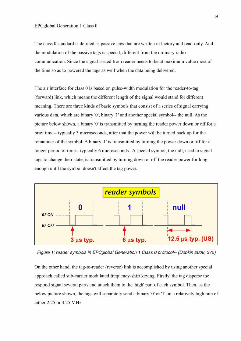
The air interface for class 0 is based on pulse-width modulation for the reader-to-tag

(forward) link, which means the different length of the signal would stand for different

meaning. There are three kinds of basic symbols that consist of a series of signal carrying

various data, which are binary '0', binary '1' and another special symbol-- the null. As the

picture below shown, a binary '0' is transmitted by turning the reader power down or off for a

brief time-- typically 3 microseconds, after that the power will be turned back up for the

remainder of the symbol; A binary '1' is transmitted by turning the power down or off for a

longer period of time-- typically 6 microseconds. A special symbol, the null, used to signal

tags to change their state, is transmitted by turning down or off the reader power for long

enough until the symbol doesn't affect the tag power.

Figure 1: reader symbols in EPCglobal Generation 1 Class 0 protocol-- (Dobkin 2008, 375)

On the other hand, the tag-to-reader (reverse) link is accomplished by using another special

approach called sub-carrier modulated frequency-shift keying. Firstly, the tag disperse the

respond signal several parts and attach them to the 'high' part of each symbol. Then, as the

below picture shown, the tags will separately send a binary '0' or '1' on a relatively high rate of

either 2.25 or 3.25 MHz.

14

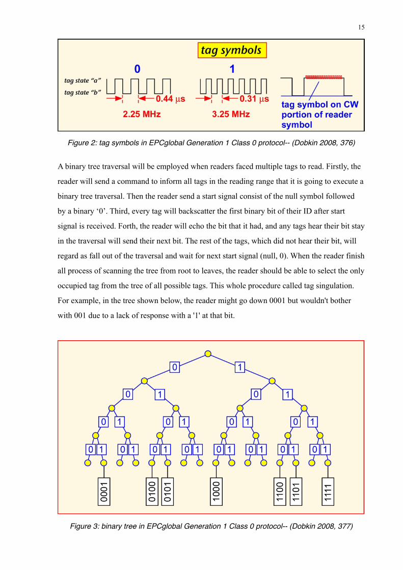
Figure 2: tag symbols in EPCglobal Generation 1 Class 0 protocol-- (Dobkin 2008, 376)

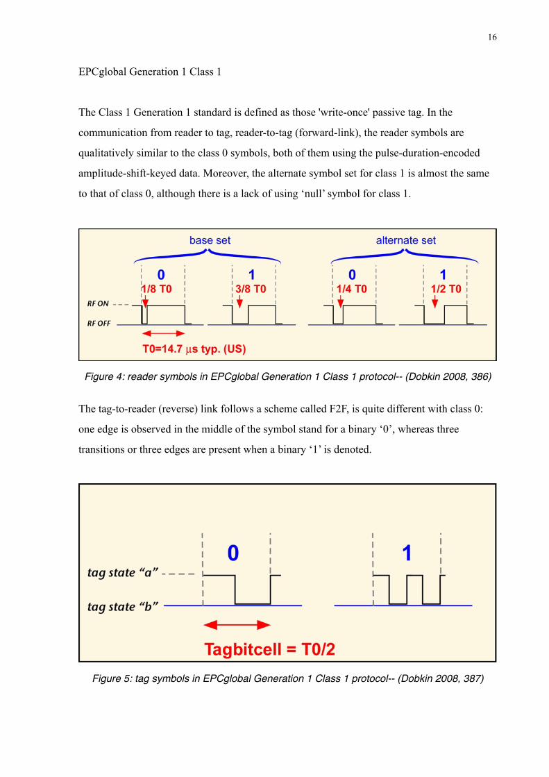
A binary tree traversal will be employed when readers faced multiple tags to read. Firstly, the

reader will send a command to inform all tags in the reading range that it is going to execute a

binary tree traversal. Then the reader send a start signal consist of the null symbol followed

by a binary ‘0’. Third, every tag will backscatter the first binary bit of their ID after start

signal is received. Forth, the reader will echo the bit that it had, and any tags hear their bit stay

in the traversal will send their next bit. The rest of the tags, which did not hear their bit, will

regard as fall out of the traversal and wait for next start signal (null, 0). When the reader finish

all process of scanning the tree from root to leaves, the reader should be able to select the only

occupied tag from the tree of all possible tags. This whole procedure called tag singulation.

For example, in the tree shown below, the reader might go down 0001 but wouldn't bother

with 001 due to a lack of response with a '1' at that bit.

Figure 3: binary tree in EPCglobal Generation 1 Class 0 protocol-- (Dobkin 2008, 377)

15

EPCglobal Generation 1 Class 1

The Class 1 Generation 1 standard is defined as those 'write-once' passive tag. In the

communication from reader to tag, reader-to-tag (forward-link), the reader symbols are

qualitatively similar to the class 0 symbols, both of them using the pulse-duration-encoded

amplitude-shift-keyed data. Moreover, the alternate symbol set for class 1 is almost the same

to that of class 0, although there is a lack of using ‘null’ symbol for class 1.

Figure 4: reader symbols in EPCglobal Generation 1 Class 1 protocol-- (Dobkin 2008, 386)

The tag-to-reader (reverse) link follows a scheme called F2F, is quite different with class 0:

one edge is observed in the middle of the symbol stand for a binary ‘0’, whereas three

transitions or three edges are present when a binary ‘1’ is denoted.

Figure 5: tag symbols in EPCglobal Generation 1 Class 1 protocol-- (Dobkin 2008, 387)

16

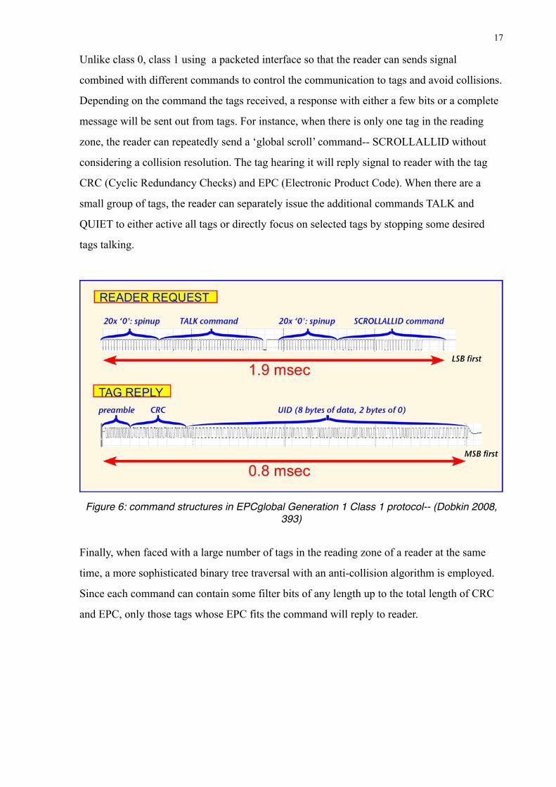
Unlike class 0, class 1 using a packeted interface so that the reader can sends signal

combined with different commands to control the communication to tags and avoid collisions.

Depending on the command the tags received, a response with either a few bits or a complete

message will be sent out from tags. For instance, when there is only one tag in the reading

zone, the reader can repeatedly send a ‘global scroll’ command-- SCROLLALLID without

considering a collision resolution. The tag hearing it will reply signal to reader with the tag

CRC (Cyclic Redundancy Checks) and EPC (Electronic Product Code). When there are a

small group of tags, the reader can separately issue the additional commands TALK and

QUIET to either active all tags or directly focus on selected tags by stopping some desired

tags talking.

Figure 6: command structures in EPCglobal Generation 1 Class 1 protocol-- (Dobkin 2008, 393)

Finally, when faced with a large number of tags in the reading zone of a reader at the same

time, a more sophisticated binary tree traversal with an anti-collision algorithm is employed.

Since each command can contain some filter bits of any length up to the total length of CRC

and EPC, only those tags whose EPC fits the command will reply to reader.

17

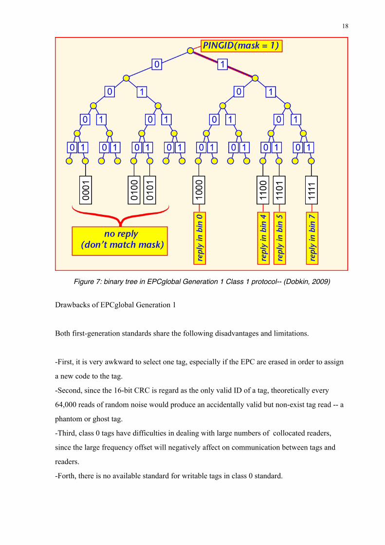
Figure 7: binary tree in EPCglobal Generation 1 Class 1 protocol-- (Dobkin, 2009)

Drawbacks of EPCglobal Generation 1

Both first-generation standards share the following disadvantages and limitations.

-First, it is very awkward to select one tag, especially if the EPC are erased in order to assign

a new code to the tag.

-Second, since the 16-bit CRC is regard as the only valid ID of a tag, theoretically every

64,000 reads of random noise would produce an accidentally valid but non-exist tag read -- a

phantom or ghost tag.

-Third, class 0 tags have difficulties in dealing with large numbers of collocated readers,

since the large frequency offset will negatively affect on communication between tags and

readers.

-Forth, there is no available standard for writable tags in class 0 standard.

18

-Fifth, the singulation procedure of class 1 is relatively time-consuming particularly when

facing a large number of tags in the reading zone.

-Sixth, both class 0 and class 1 have the problems with the late arrivals, which describes a

situation that tags come into the reading zone after the inventory has already started.

Finally, with those disadvantages and limitations, class 0 and class 1 are mutually

incompatible and people begin to seek another resolution which is good enough to widely

used in every applications with a satisfied performance.

2.4.3 EPCglobal Class 1 Generation 2 (ISO 18000-6C)

By realizing those problems above, the EPCglobal Hardware Action Group in early 2004

started work on a second-generation standard focused on fixing the problems of first-

generation left.

Finally in early 2005, The Class 1 Generation 2 standard was born, which is now also ratified

by the International Organization for Standardization (ISO) as ISO 18000-6C.

The Gen 2 standard bring significant improvement in many aspect, although it completely

incompatible with Gen 1 readers and tags.

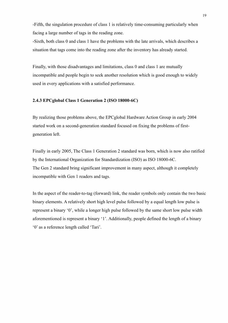
In the aspect of the reader-to-tag (forward) link, the reader symbols only contain the two basic

binary elements. A relatively short high level pulse followed by a equal length low pulse is

represent a binary ‘0’, while a longer high pulse followed by the same short low pulse width

aforementioned is represent a binary ‘1’. Additionally, people defined the length of a binary

‘0’ as a reference length called ‘Tari’.

19

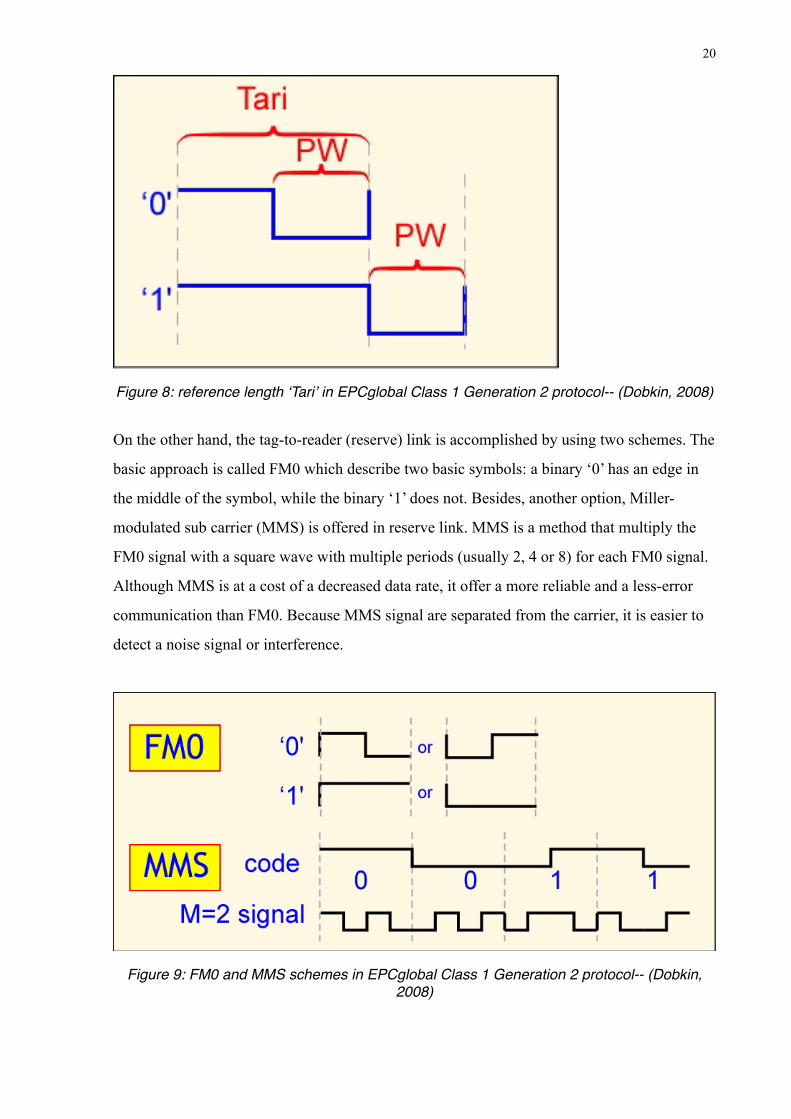
Figure 8: reference length ʻTariʼ in EPCglobal Class 1 Generation 2 protocol-- (Dobkin, 2008)

On the other hand, the tag-to-reader (reserve) link is accomplished by using two schemes. The

basic approach is called FM0 which describe two basic symbols: a binary ‘0’ has an edge in

the middle of the symbol, while the binary ‘1’ does not. Besides, another option, Miller-

modulated sub carrier (MMS) is offered in reserve link. MMS is a method that multiply the

FM0 signal with a square wave with multiple periods (usually 2, 4 or 8) for each FM0 signal.

Although MMS is at a cost of a decreased data rate, it offer a more reliable and a less-error

communication than FM0. Because MMS signal are separated from the carrier, it is easier to

detect a noise signal or interference.

Figure 9: FM0 and MMS schemes in EPCglobal Class 1 Generation 2 protocol-- (Dobkin, 2008)

20

Like Gen 1, the communication between tags and readers of Gen 2 also using a packeted

interface while the packet contents are rather different from the former generation.

Instead of a binary tree in Gen 1, Gen 2 standard use inventory operations based on slotted

Aloha to resolve the collision. A QUERY command issued by reader cause each tag rolls a

many-sided die and the number of sides has already been set by the reader. A tag will respond

immediately whenever a ‘0’ is rolled, otherwise the tag will save the numbers and replies

nothing if other numbers is rolled. After that, a QUERY REP command will be sent from

reader when either it received a reply or nothing. This command will call all the numbers

saved in the tag to decrease by 1. When it count down to the value of 0, the tag will respond

immediately. If this system work properly, one and only one tag will reply to most of the

QUERY REP commands.

Also a 16-bit random number RN16 sent from tag is used as a method of acknowledgement

during this procedure. The reader will echo the RN16 they heard from the tag, so that the tag

could continue the conversation and begin to sent their useful information such like EPC,

CRC along with some protocol control bits (PC).

21

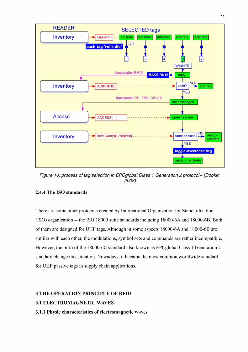
Figure 10: process of tag selection in EPCglobal Class 1 Generation 2 protocol-- (Dobkin, 2008)

2.4.4 The ISO standards

There are some other protocols created by International Organization for Standardization

(ISO) organization -- the ISO 18000 suite standards including 18000-6A and 18000-6B. Both

of them are designed for UHF tags. Although in some aspects 18000-6A and 18000-6B are

similar with each other, the modulations, symbol sets and commands are rather incompatible.

However, the birth of the 18000-6C standard also known as EPCglobal Class 1 Generation 2

standard change this situation. Nowadays, it became the most common worldwide standard

for UHF passive tags in supply chain applications.

3 THE OPERATION PRINCIPLE OF RFID

3.1 ELECTROMAGNETIC WAVES

3.1.1 Physic characteristics of electromagnetic waves

22

Electromagnetic waves essentially describes the same object as electromagnetic field but in a

dynamic fashion. In other wards, the two elements, electricity and magnetism, are just like

two different aspects of one item. A spatially-changing electric field will cause a time-

changing magnetic field, and vice versa. Therefore, the oscillation of either electric field or

magnetic field will cause a improvement to another. This oscillation field finally bring out the

product called electromagnetic waves.

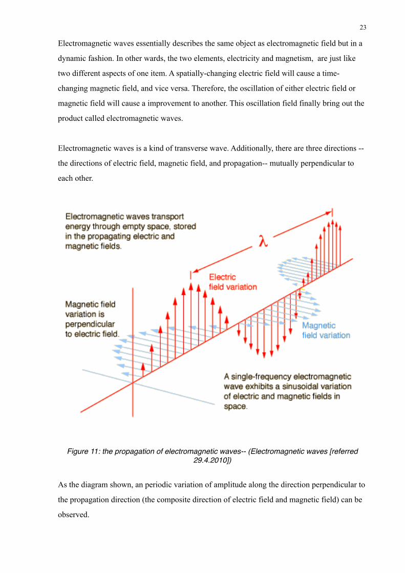
Electromagnetic waves is a kind of transverse wave. Additionally, there are three directions --

the directions of electric field, magnetic field, and propagation-- mutually perpendicular to

each other.

Figure 11: the propagation of electromagnetic waves-- (Electromagnetic waves [referred 29.4.2010])

As the diagram shown, an periodic variation of amplitude along the direction perpendicular to

the propagation direction (the composite direction of electric field and magnetic field) can be

observed.

23

The propagation speed of electromagnetic waves is coincided with the measure speed of light

c (3*10⁸ m/s). The frequency of a wave f describes the rate of oscillation. And the wavelength

λ stand for the distance between two adjacent crests or troughs of a wave. These three variable

followed an equation:

c = λf

3.1.2 When electromagnetic waves travel through space

When electromagnetic waves travel, they may have some interaction with objects and the

media where they transmitted. In this case, three situations can be expected -- reflected,

refracted or diffracted. All of them could lead to a change of the wave direction and reach an

unexpected place where is impossible for waves to get if they traveled in a line.

Reflection

With an essentially same principle of light reflection caused by a mirror, electromagnetic

wave can be reflected by several surface such as the ocean, land buildings and so on. When

the reflection happened, there is always a pair of equal angles -- the angles of incidence and

reflection. Additionally, although in theory the strength of the signal will not be affected by

the reflection, in practice, there will be some normally loss of the signal, either due to

absorption or a result of signal penetrating into the medium.

Refraction

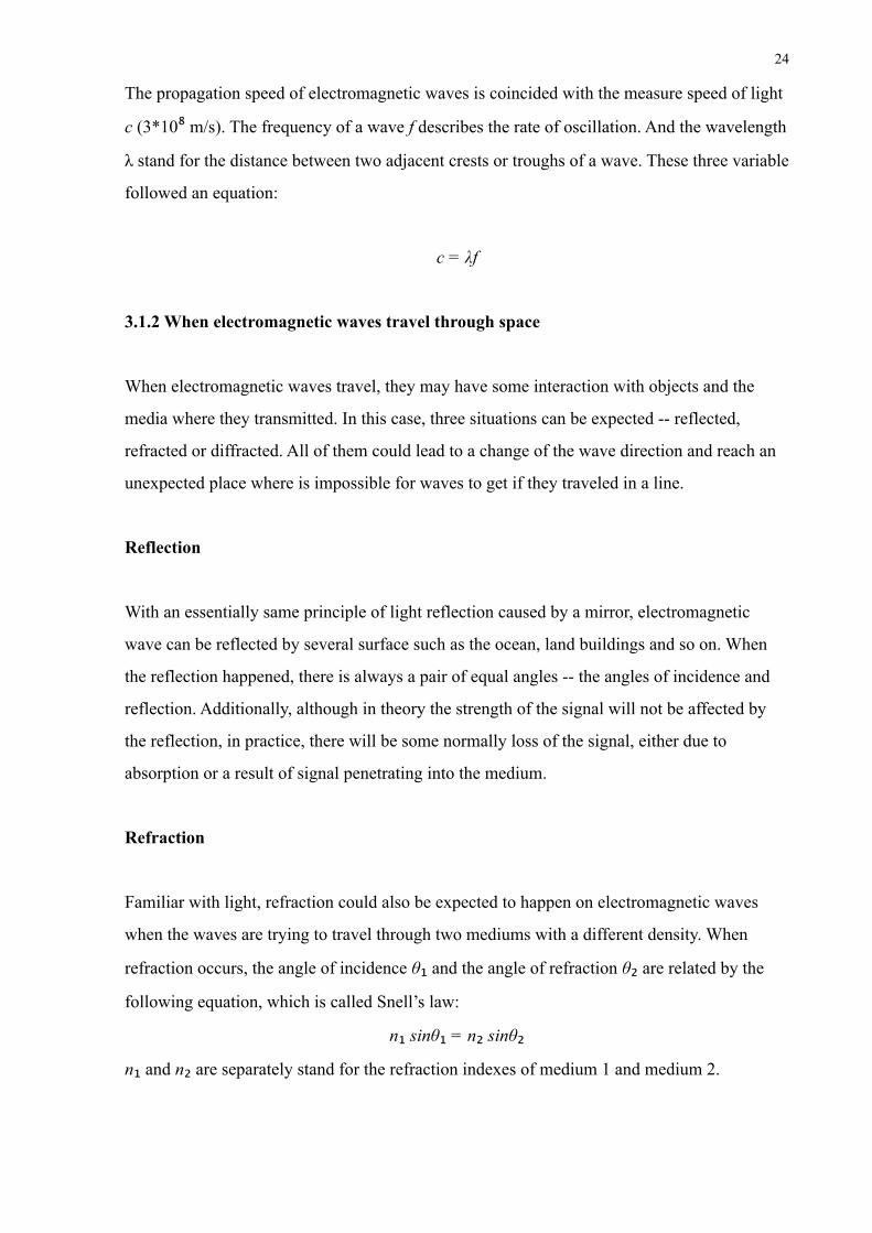
Familiar with light, refraction could also be expected to happen on electromagnetic waves

when the waves are trying to travel through two mediums with a different density. When

refraction occurs, the angle of incidence θ₁ and the angle of refraction θ₂ are related by the

following equation, which is called Snell’s law:

n₁ sinθ₁ = n₂ sinθ₂

n₁ and n₂ are separately stand for the refraction indexes of medium 1 and medium 2.

24

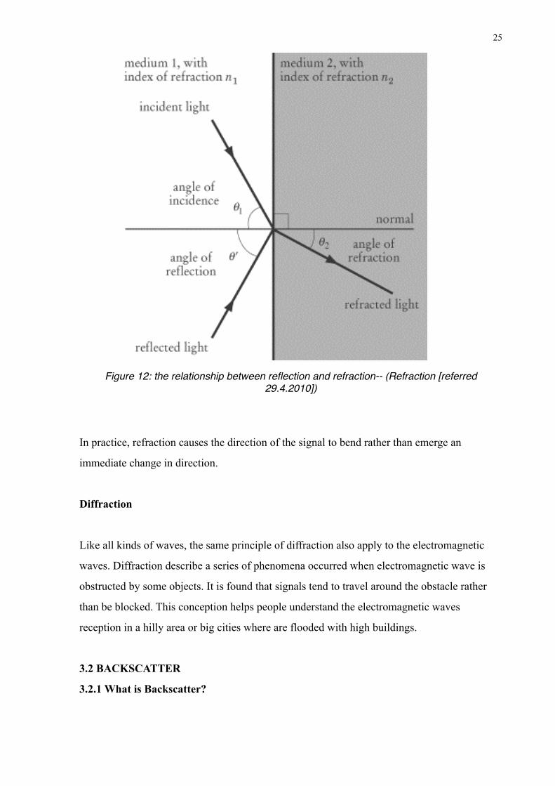
Figure 12: the relationship between reflection and refraction-- (Refraction [referred 29.4.2010])

In practice, refraction causes the direction of the signal to bend rather than emerge an

immediate change in direction.

Diffraction

Like all kinds of waves, the same principle of diffraction also apply to the electromagnetic

waves. Diffraction describe a series of phenomena occurred when electromagnetic wave is

obstructed by some objects. It is found that signals tend to travel around the obstacle rather

than be blocked. This conception helps people understand the electromagnetic waves

reception in a hilly area or big cities where are flooded with high buildings.

3.2 BACKSCATTER

3.2.1 What is Backscatter?

25

In the aspect of physics, backscatter stand for the reflection of waves, particles, or signals

back to the direction where they came. The reflection mentioned here is a diffuse reflection

due to an uneven or granular surface, which opposed to specular reflection such as light

reflected by a mirror.

Figure 13: difference between specular reflection and diffuse reflection-- (Diffuse refection [referred 30.4.2010])

3.2.2 Backscatter in RFID

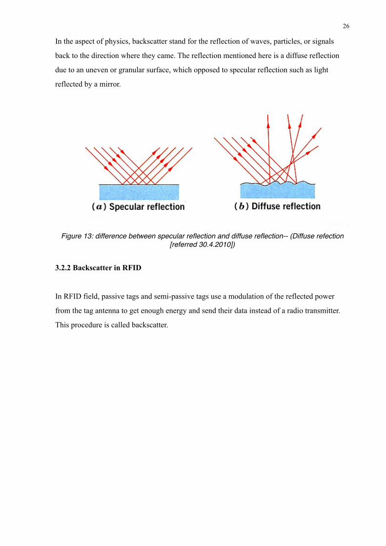
In RFID field, passive tags and semi-passive tags use a modulation of the reflected power

from the tag antenna to get enough energy and send their data instead of a radio transmitter.

This procedure is called backscatter.

26

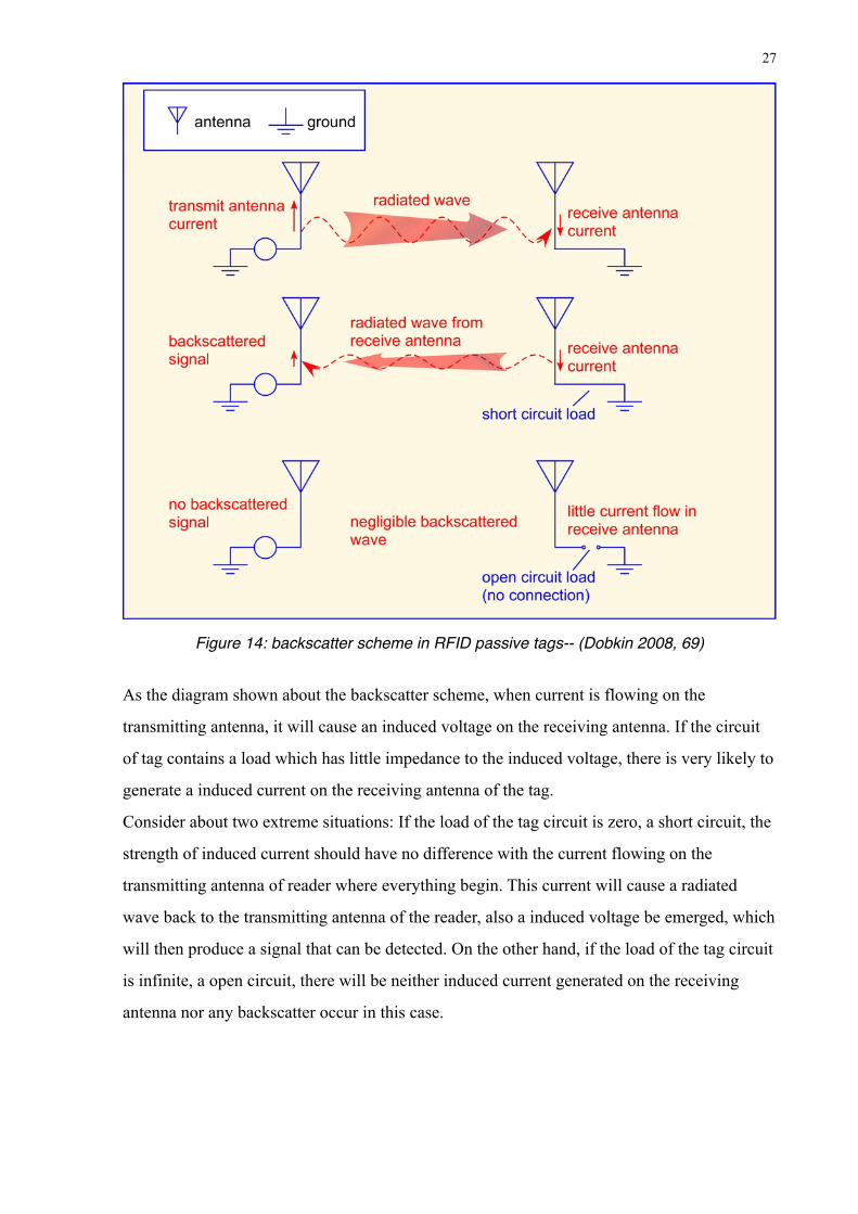
Figure 14: backscatter scheme in RFID passive tags-- (Dobkin 2008, 69)

As the diagram shown about the backscatter scheme, when current is flowing on the

transmitting antenna, it will cause an induced voltage on the receiving antenna. If the circuit

of tag contains a load which has little impedance to the induced voltage, there is very likely to

generate a induced current on the receiving antenna of the tag.

Consider about two extreme situations: If the load of the tag circuit is zero, a short circuit, the

strength of induced current should have no difference with the current flowing on the

transmitting antenna of reader where everything begin. This current will cause a radiated

wave back to the transmitting antenna of the reader, also a induced voltage be emerged, which

will then produce a signal that can be detected. On the other hand, if the load of the tag circuit

is infinite, a open circuit, there will be neither induced current generated on the receiving

antenna nor any backscatter occur in this case.

27

3.3 TRANSMITTING PROCEDURE

3.3.1 A panorama of RFID communication

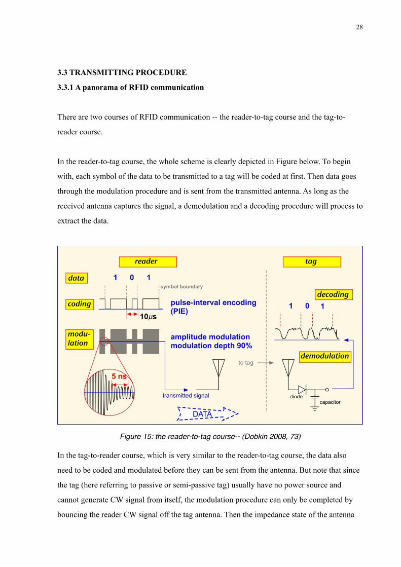
There are two courses of RFID communication -- the reader-to-tag course and the tag-to-

reader course.

In the reader-to-tag course, the whole scheme is clearly depicted in Figure below. To begin

with, each symbol of the data to be transmitted to a tag will be coded at first. Then data goes

through the modulation procedure and is sent from the transmitted antenna. As long as the

received antenna captures the signal, a demodulation and a decoding procedure will process to

extract the data.

Figure 15: the reader-to-tag course-- (Dobkin 2008, 73)

In the tag-to-reader course, which is very similar to the reader-to-tag course, the data also

need to be coded and modulated before they can be sent from the antenna. But note that since

the tag (here referring to passive or semi-passive tag) usually have no power source and

cannot generate CW signal from itself, the modulation procedure can only be completed by

bouncing the reader CW signal off the tag antenna. Then the impedance state of the antenna

28

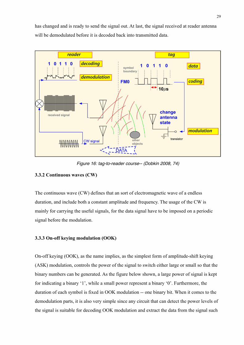
has changed and is ready to send the signal out. At last, the signal received at reader antenna

will be demodulated before it is decoded back into transmitted data.

Figure 16: tag-to-reader course-- (Dobkin 2008, 74)

3.3.2 Continuous waves (CW)

The continuous wave (CW) defines that an sort of electromagnetic wave of a endless

duration, and include both a constant amplitude and frequency. The usage of the CW is

mainly for carrying the useful signals, for the data signal have to be imposed on a periodic

signal before the modulation.

3.3.3 On-off keying modulation (OOK)

On-off keying (OOK), as the name implies, as the simplest form of amplitude-shift keying

(ASK) modulation, controls the power of the signal to switch either large or small so that the

binary numbers can be generated. As the figure below shown, a large power of signal is kept

for indicating a binary ‘1’, while a small power represent a binary ‘0’. Furthermore, the

duration of each symbol is fixed in OOK modulation -- one binary bit. When it comes to the

demodulation parts, it is also very simple since any circuit that can detect the power levels of

the signal is suitable for decoding OOK modulation and extract the data from the signal such

29

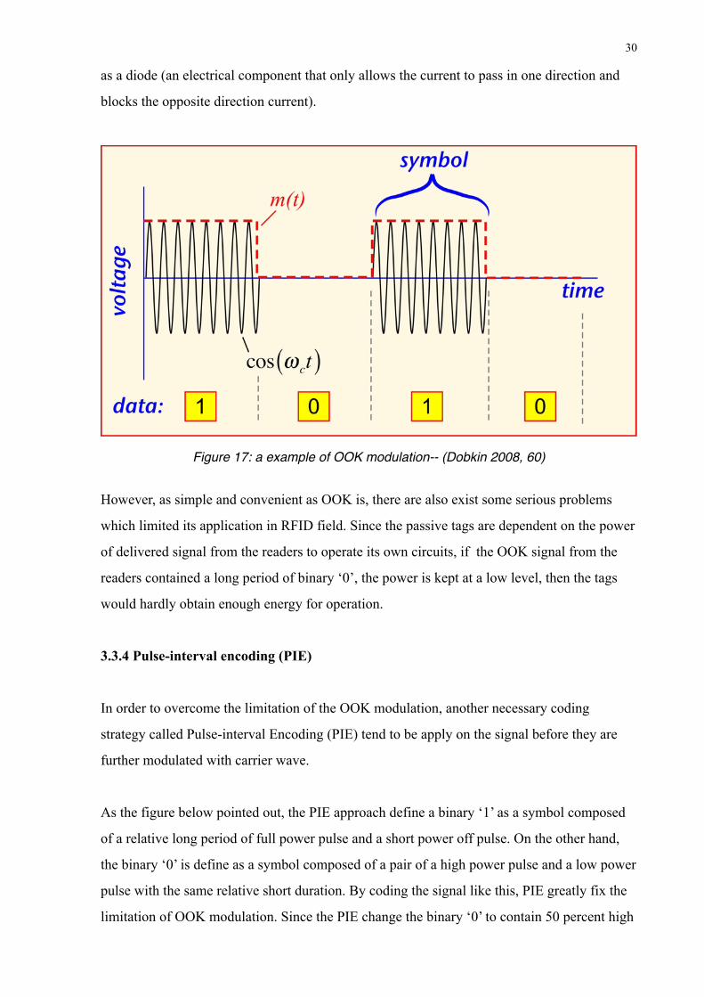
as a diode (an electrical component that only allows the current to pass in one direction and

blocks the opposite direction current).

Figure 17: a example of OOK modulation-- (Dobkin 2008, 60)

However, as simple and convenient as OOK is, there are also exist some serious problems

which limited its application in RFID field. Since the passive tags are dependent on the power

of delivered signal from the readers to operate its own circuits, if the OOK signal from the

readers contained a long period of binary ‘0’, the power is kept at a low level, then the tags

would hardly obtain enough energy for operation.

3.3.4 Pulse-interval encoding (PIE)

In order to overcome the limitation of the OOK modulation, another necessary coding

strategy called Pulse-interval Encoding (PIE) tend to be apply on the signal before they are

further modulated with carrier wave.

As the figure below pointed out, the PIE approach define a binary ‘1’ as a symbol composed

of a relative long period of full power pulse and a short power off pulse. On the other hand,

the binary ‘0’ is define as a symbol composed of a pair of a high power pulse and a low power

pulse with the same relative short duration. By coding the signal like this, PIE greatly fix the

limitation of OOK modulation. Since the PIE change the binary ‘0’ to contain 50 percent high

30

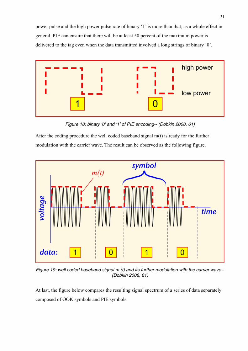
power pulse and the high power pulse rate of binary ‘1’ is more than that, as a whole effect in

general, PIE can ensure that there will be at least 50 percent of the maximum power is

delivered to the tag even when the data transmitted involved a long strings of binary ‘0’.

Figure 18: binary ʻ0ʼ and ʻ1ʼ of PIE encoding-- (Dobkin 2008, 61)

After the coding procedure the well coded baseband signal m(t) is ready for the further

modulation with the carrier wave. The result can be observed as the following figure.

Figure 19: well coded baseband signal m (t) and its further modulation with the carrier wave-- (Dobkin 2008, 61)

At last, the figure below compares the resulting signal spectrum of a series of data separately

composed of OOK symbols and PIE symbols.

31

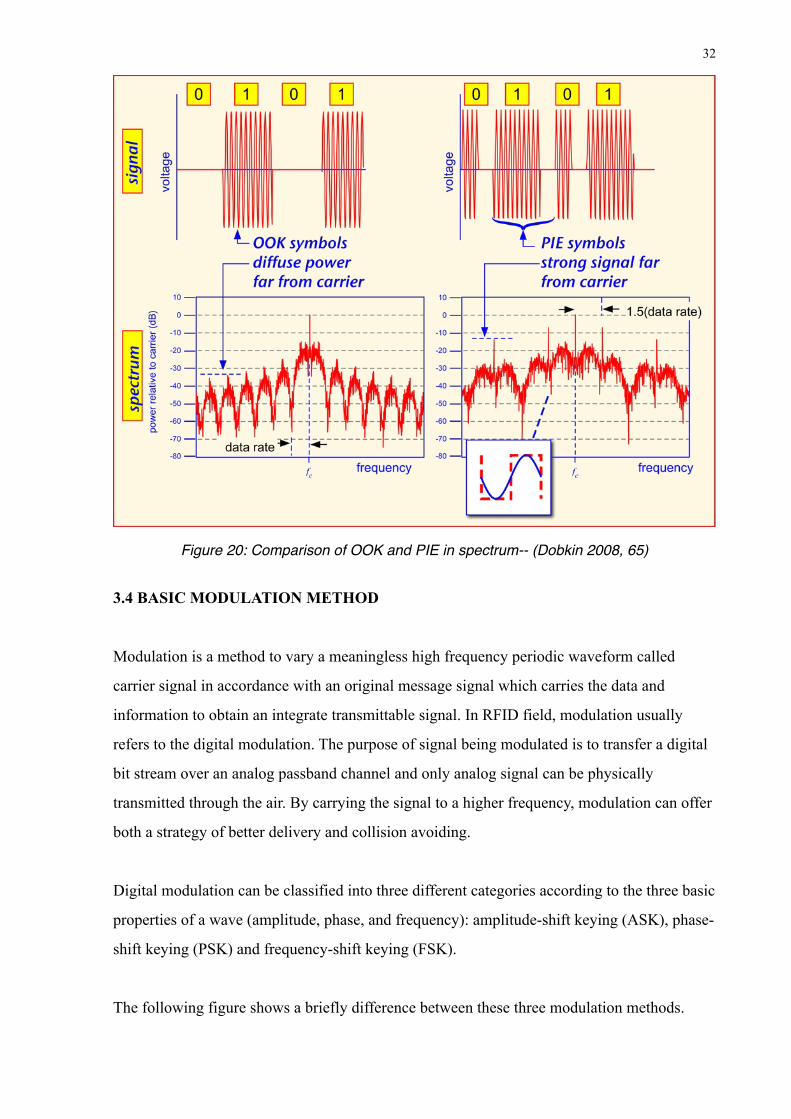
Figure 20: Comparison of OOK and PIE in spectrum-- (Dobkin 2008, 65)

3.4 BASIC MODULATION METHOD

Modulation is a method to vary a meaningless high frequency periodic waveform called

carrier signal in accordance with an original message signal which carries the data and

information to obtain an integrate transmittable signal. In RFID field, modulation usually

refers to the digital modulation. The purpose of signal being modulated is to transfer a digital

bit stream over an analog passband channel and only analog signal can be physically

transmitted through the air. By carrying the signal to a higher frequency, modulation can offer

both a strategy of better delivery and collision avoiding.

Digital modulation can be classified into three different categories according to the three basic

properties of a wave (amplitude, phase, and frequency): amplitude-shift keying (ASK), phase-

shift keying (PSK) and frequency-shift keying (FSK).

The following figure shows a briefly difference between these three modulation methods.

32

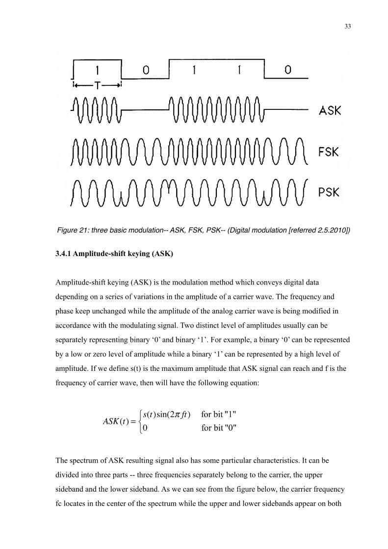
Figure 21: three basic modulation-- ASK, FSK, PSK-- (Digital modulation [referred 2.5.2010])

3.4.1 Amplitude-shift keying (ASK)

Amplitude-shift keying (ASK) is the modulation method which conveys digital data

depending on a series of variations in the amplitude of a carrier wave. The frequency and

phase keep unchanged while the amplitude of the analog carrier wave is being modified in

accordance with the modulating signal. Two distinct level of amplitudes usually can be

separately representing binary ‘0’ and binary ‘1’. For example, a binary ‘0’ can be represented

by a low or zero level of amplitude while a binary ‘1’ can be represented by a high level of

amplitude. If we define s(t) is the maximum amplitude that ASK signal can reach and f is the

frequency of carrier wave, then will have the following equation:

The spectrum of ASK resulting signal also has some particular characteristics. It can be

divided into three parts -- three frequencies separately belong to the carrier, the upper

sideband and the lower sideband. As we can see from the figure below, the carrier frequency

fc locates in the center of the spectrum while the upper and lower sidebands appear on both

33

sides with a distance fm from the carrier frequency fc. Therefore, the frequencies of upper and

lower sidebands can be separately represented as fc+fm and fc-fm.

Figure 22: The spectrum of ASK resulting signal-- (Dobkin 2008, 59)

3.4.2 Frequency-shift keying (FSK)

Frequency-shift keying (FSK) is the modulation method which conveys digital data

depending on a series of variations in the frequency of a carrier wave while the other

properties-- amplitude and phase-- remain constant. In FSK, two different frequencies are

assigned to separately deliver a binary ‘0’ and ‘1’. Each time a change in frequency happened,

the data state will be altered to another. The FSK modulation method can be described as the

following equation:

34

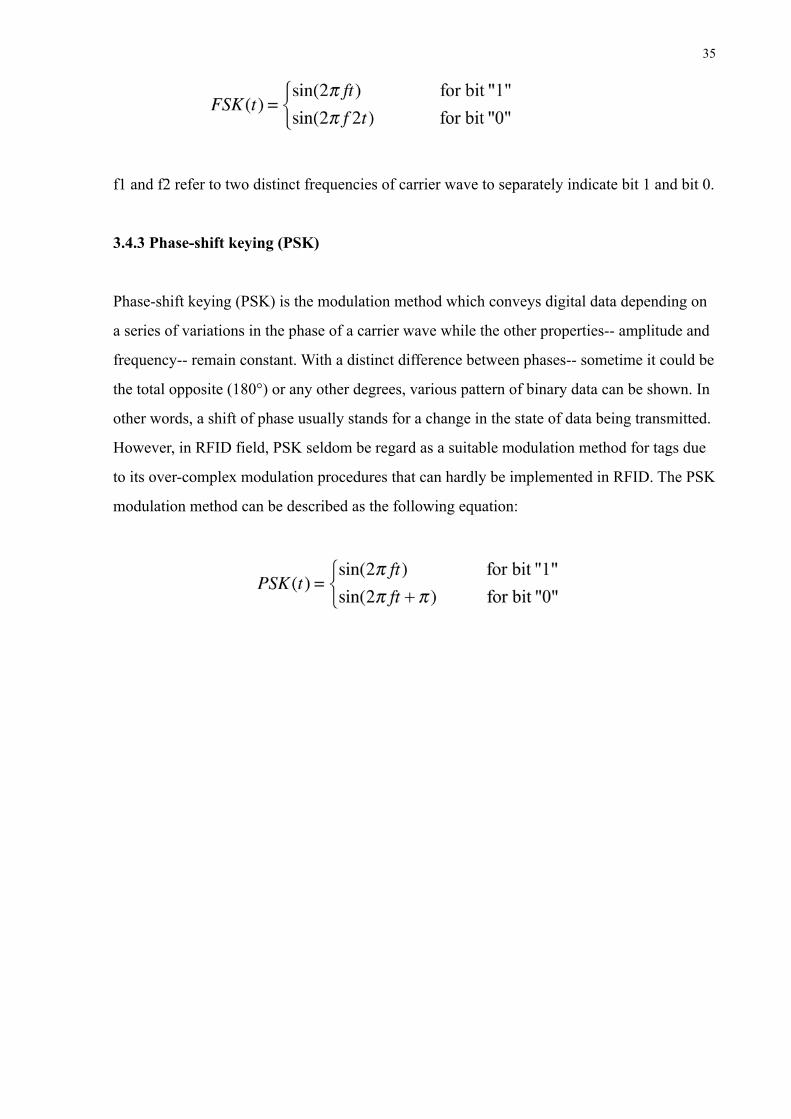
f1 and f2 refer to two distinct frequencies of carrier wave to separately indicate bit 1 and bit 0.

3.4.3 Phase-shift keying (PSK)

Phase-shift keying (PSK) is the modulation method which conveys digital data depending on

a series of variations in the phase of a carrier wave while the other properties-- amplitude and

frequency-- remain constant. With a distinct difference between phases-- sometime it could be

the total opposite (180°) or any other degrees, various pattern of binary data can be shown. In

other words, a shift of phase usually stands for a change in the state of data being transmitted.

However, in RFID field, PSK seldom be regard as a suitable modulation method for tags due

to its over-complex modulation procedures that can hardly be implemented in RFID. The PSK

modulation method can be described as the following equation:

35

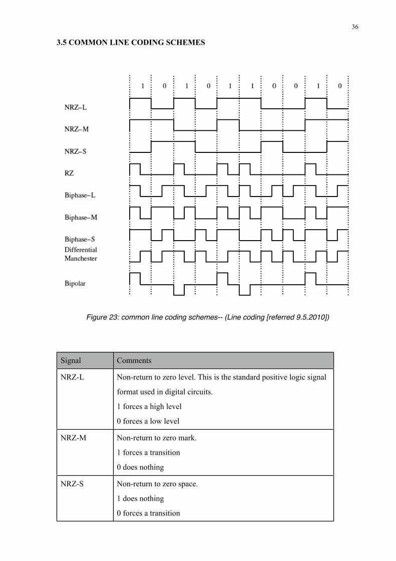
3.5 COMMON LINE CODING SCHEMES

Figure 23: common line coding schemes-- (Line coding [referred 9.5.2010])

Signal Comments

NRZ-L Non-return to zero level. This is the standard positive logic signal

format used in digital circuits.

1 forces a high level

0 forces a low level

NRZ-M Non-return to zero mark.

1 forces a transition

0 does nothing

NRZ-S Non-return to zero space.

1 does nothing

0 forces a transition

36

Signal Comments

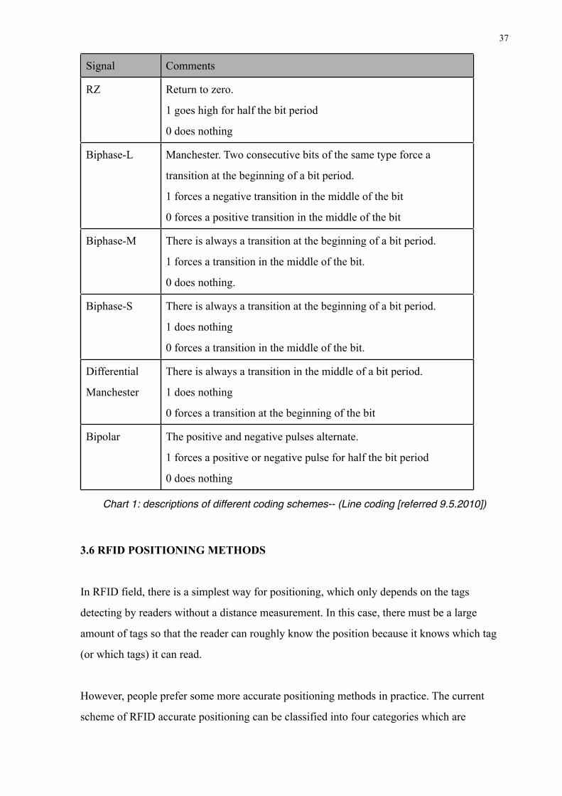
RZ Return to zero.

1 goes high for half the bit period

0 does nothing

Biphase-L Manchester. Two consecutive bits of the same type force a

transition at the beginning of a bit period.

1 forces a negative transition in the middle of the bit

0 forces a positive transition in the middle of the bit

Biphase-M There is always a transition at the beginning of a bit period.

1 forces a transition in the middle of the bit.

0 does nothing.

Biphase-S There is always a transition at the beginning of a bit period.

1 does nothing

0 forces a transition in the middle of the bit.

Differential

Manchester

There is always a transition in the middle of a bit period.

1 does nothing

0 forces a transition at the beginning of the bit

Bipolar The positive and negative pulses alternate.

1 forces a positive or negative pulse for half the bit period

0 does nothing

Chart 1: descriptions of different coding schemes-- (Line coding [referred 9.5.2010])

3.6 RFID POSITIONING METHODS

In RFID field, there is a simplest way for positioning, which only depends on the tags

detecting by readers without a distance measurement. In this case, there must be a large

amount of tags so that the reader can roughly know the position because it knows which tag

(or which tags) it can read.

However, people prefer some more accurate positioning methods in practice. The current

scheme of RFID accurate positioning can be classified into four categories which are

37

Received Signal Strength Indication (RSSI), Time of Arrival (TOA), Time Difference of

Arrival (TDoA) and Angle of Arrival (AoA).

3.6.1 Received Signal Strength Indication (RSSI)

In telecommunications, received signal strength indicator (RSSI) as a method of distance

measurement is accomplished by detecting the degradation of signal strength, since that the

level of the signal degradation is inversely proportional to the distance.

Received signal strength indicator (RSSI) scheme is relatively easy and simple to implement.

However, the accuracy cannot be guaranteed due to its vulnerability to reflection and multi-

path interference. (Received Signal Strength Indication (RSSI) [referred 16.5.2010])

3.6.2 Time of Arrival (TOA)

Time of Arrival (TOA) used to measure the distance between transmitter and receiver by

obtaining the time consumed during the signal traveling. In order to calculate the distance, the

speed of light in a certain medium (usually can be defined as vacuum in the air condition) or

the frequency of the carrier wave is required. Note that TOA uses the absolute time, which

means the exact time when the signal departure and arrival should be known. Because the

accuracy of time is very important in TOA method, a synchronous time on both a receiver and

transmitter becomes extremely necessary which also adds the complication to the

implementation. (Time of Arrival (TOA) [referred 16.5.2010])

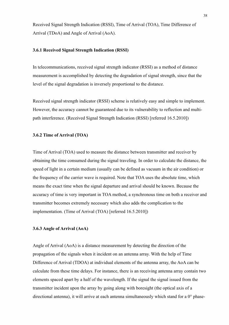
3.6.3 Angle of Arrival (AoA)

Angle of Arrival (AoA) is a distance measurement by detecting the direction of the

propagation of the signals when it incident on an antenna array. With the help of Time

Difference of Arrival (TDOA) at individual elements of the antenna array, the AoA can be

calculate from these time delays. For instance, there is an receiving antenna array contain two

elements spaced apart by a half of the wavelength. If the signal the signal issued from the

transmitter incident upon the array by going along with boresight (the optical axis of a

directional antenna), it will arrive at each antenna simultaneously which stand for a 0° phase-

38

difference measured between the two antenna elements, equivalent to a 0° AoA. In this way, a

180° phase difference will be generated between the two antenna elements due to a broadside

incident signal and the half wavelength distance between which correspond to a 90° AoA.

Figure 24: a receiving antenna array contains two elements spaced apart by a half of the wavelength-- (Angle of Arrival (AoA) [referred 16.5.2010])

In practice, however, AOA is very expensive and high power consuming since using the

antenna array instead of regular antenna. Plus, AOA is also not stable enough to the

environment conditions. (Angle of Arrival (AoA) [referred 16.5.2010])

3.6.4 Time Difference of Arrival (TDoA)

Time Difference of Arrival (TDoA) is similar to the TOA technique, the only difference

between them is that the time concerned by TDoA is relative time instead of the absolute one,

which means the mainly job in TDoA is to measure the time difference between the signals

departure and arrival with a known velocity.

However, the time difference can be very small if the distance differences are small. For

instance, a distance difference of 0.3 m equals to a time difference of 1 ns, or 10⁻⁹ s. It is so

39

difficult to synchronize the receivers to ensure such small time differences can be measured.

Therefore an alternative solution for synchronization comes out-- there can be some reference

tags at well-known and fixed positions help readers synchronizing. (Bouet [referred

16.5.2010])

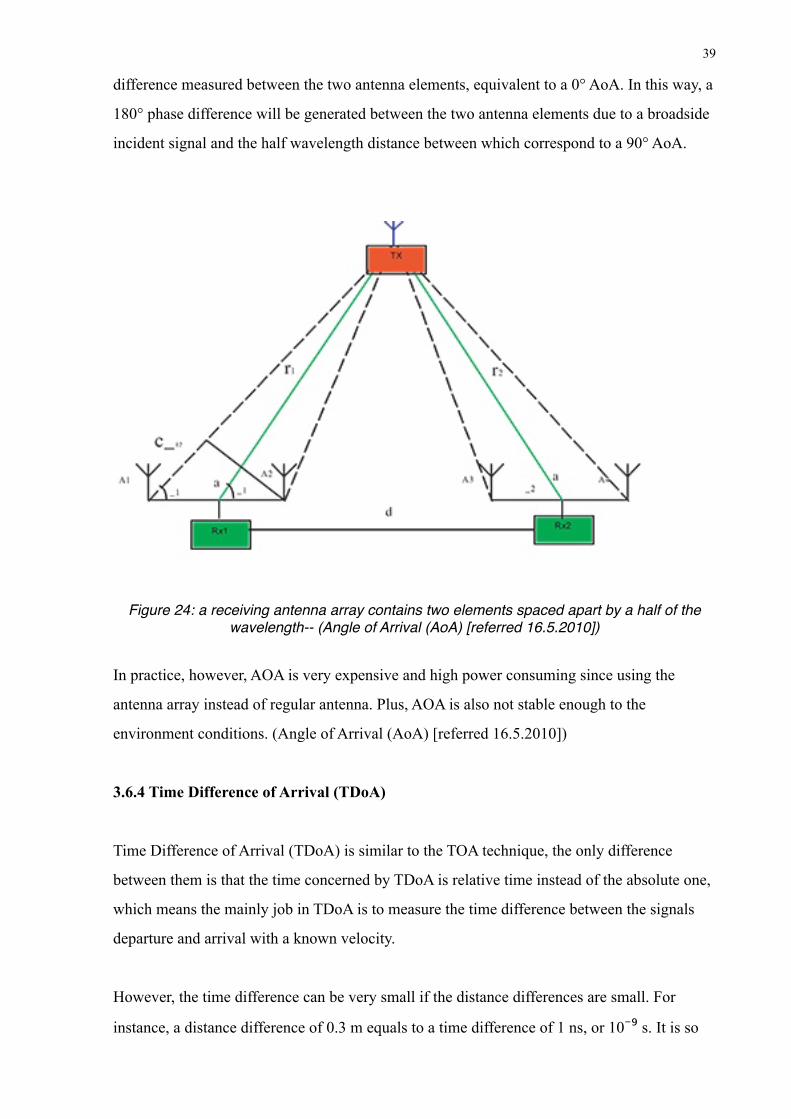
Next, I will discuss the algorithms and operating schemes of TDOA method:

Figure 25: working principle of TDoA scheme-- (Time Difference of Arrival (TDoA) [referred 16.5.2010])

Consider an emitter (E in Figure) as an unknown location vector

E = (x, y, z)

which need to be located. The source is within range of N receivers at known locations:

40

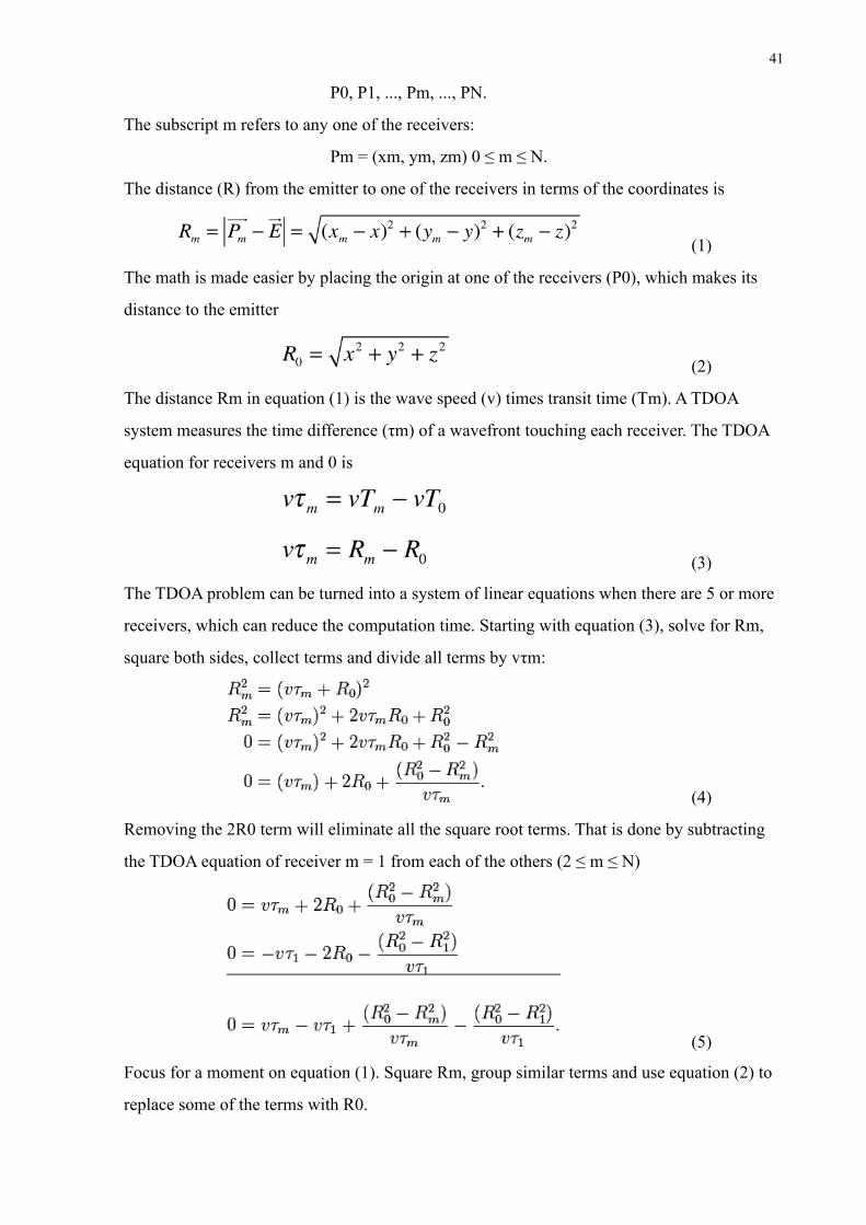
P0, P1, ..., Pm, ..., PN.

The subscript m refers to any one of the receivers:

Pm = (xm, ym, zm) 0 ≤ m ≤ N.

The distance (R) from the emitter to one of the receivers in terms of the coordinates is

(1)

The math is made easier by placing the origin at one of the receivers (P0), which makes its

distance to the emitter

(2)

The distance Rm in equation (1) is the wave speed (v) times transit time (Tm). A TDOA

system measures the time difference (τm) of a wavefront touching each receiver. The TDOA

equation for receivers m and 0 is

(3)

The TDOA problem can be turned into a system of linear equations when there are 5 or more

receivers, which can reduce the computation time. Starting with equation (3), solve for Rm,

square both sides, collect terms and divide all terms by vτm:

(4)

Removing the 2R0 term will eliminate all the square root terms. That is done by subtracting

the TDOA equation of receiver m = 1 from each of the others (2 ≤ m ≤ N)

(5)

Focus for a moment on equation (1). Square Rm, group similar terms and use equation (2) to

replace some of the terms with R0.

41

(6)

Combine equations (5) and (6), and write as a set of linear equation of the unknown emitter

location x,y,z

(7)

Use equation (7) to generate the four constants Am,Bm,Cm,Dm from measured distances and

time for each receiver 2 ≤ m ≤ N. This will be a set of N-2 homogeneous linear equations. As

long as the measurement value (τm) is accurate, the unknown emitter location x,y,z can be

perfectly calculated.(Time Difference of Arrival (TDoA) [referred 16.5.2010])

4 EXPERIMENT

4.1 1-BIT TAG EXPERIMENT

4.1.1 Experiment purpose

1-bit tags are widely used in commercial purpose such as merchandises security system, for

its admirably simple physical structure and a really cheap cost. Often, they are attached on the

merchandises and are hard to remove without a specific tool. Whenever the tags go through

the big antenna located at the entrance, it will be active and trigger the alarm. In this way, it

contributes a lot to keep merchandises from being stolen and saves the manpower and

financial resources to a huge extent.

This experiment designed for demonstrate the working principle of 1-bit tag with an

understanding of its composition and functions of different the component of this tag.

4.1.2 Working principles

42

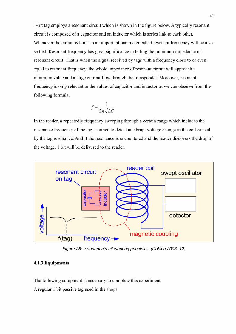
1-bit tag employs a resonant circuit which is shown in the figure below. A typically resonant

circuit is composed of a capacitor and an inductor which is series link to each other.

Whenever the circuit is built up an important parameter called resonant frequency will be also

settled. Resonant frequency has great significance in telling the minimum impedance of

resonant circuit. That is when the signal received by tags with a frequency close to or even

equal to resonant frequency, the whole impedance of resonant circuit will approach a

minimum value and a large current flow through the transponder. Moreover, resonant

frequency is only relevant to the values of capacitor and inductor as we can observe from the

following formula.

In the reader, a repeatedly frequency sweeping through a certain range which includes the

resonance frequency of the tag is aimed to detect an abrupt voltage change in the coil caused

by the tag resonance. And if the resonance is encountered and the reader discovers the drop of

the voltage, 1 bit will be delivered to the reader.

Figure 26: resonant circuit working principle-- (Dobkin 2008, 12)

4.1.3 Equipments

The following equipment is necessary to complete this experiment:

A regular 1 bit passive tag used in the shops.

43

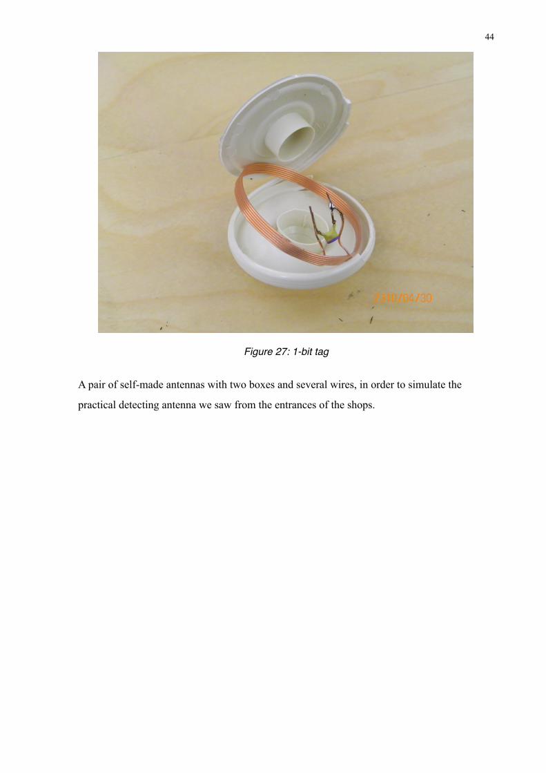
Figure 27: 1-bit tag

A pair of self-made antennas with two boxes and several wires, in order to simulate the

practical detecting antenna we saw from the entrances of the shops.

44

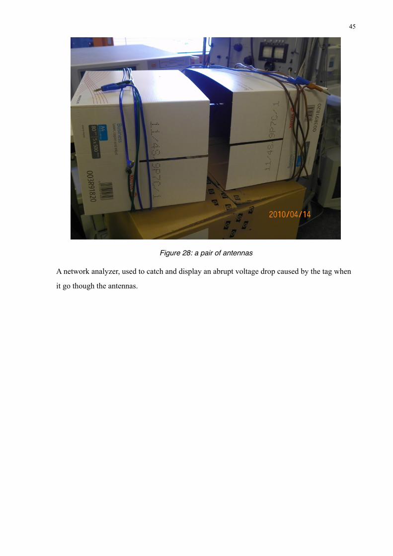
Figure 28: a pair of antennas

A network analyzer, used to catch and display an abrupt voltage drop caused by the tag when

it go though the antennas.

45

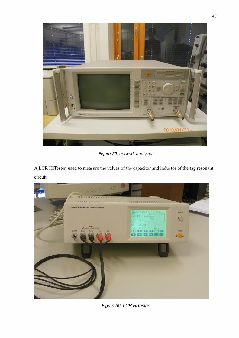
Figure 29: network analyzer

A LCR HiTester, used to measure the values of the capacitor and inductor of the tag resonant

circuit.

Figure 30: LCR HiTester

46

4.1.4 Experiment procedures

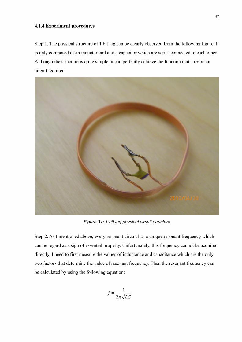
Step 1. The physical structure of 1 bit tag can be clearly observed from the following figure. It

is only composed of an inductor coil and a capacitor which are series connected to each other.

Although the structure is quite simple, it can perfectly achieve the function that a resonant

circuit required.

Figure 31: 1-bit tag physical circuit structure

Step 2. As I mentioned above, every resonant circuit has a unique resonant frequency which

can be regard as a sign of essential property. Unfortunately, this frequency cannot be acquired

directly, I need to first measure the values of inductance and capacitance which are the only

two factors that determine the value of resonant frequency. Then the resonant frequency can

be calculated by using the following equation:

47

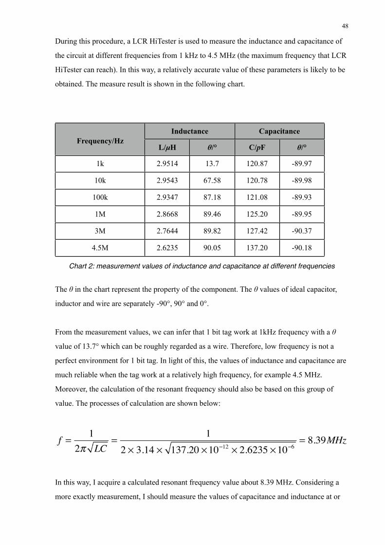
During this procedure, a LCR HiTester is used to measure the inductance and capacitance of

the circuit at different frequencies from 1 kHz to 4.5 MHz (the maximum frequency that LCR

HiTester can reach). In this way, a relatively accurate value of these parameters is likely to be

obtained. The measure result is shown in the following chart.

Frequency/HzInductanceInductance CapacitanceCapacitance

Frequency/HzL/µH θ/° C/pF θ/°

1k 2.9514 13.7 120.87 -89.97

10k 2.9543 67.58 120.78 -89.98

100k 2.9347 87.18 121.08 -89.93

1M 2.8668 89.46 125.20 -89.95

3M 2.7644 89.82 127.42 -90.37

4.5M 2.6235 90.05 137.20 -90.18

Chart 2: measurement values of inductance and capacitance at different frequencies

The θ in the chart represent the property of the component. The θ values of ideal capacitor,

inductor and wire are separately -90°, 90° and 0°.

From the measurement values, we can infer that 1 bit tag work at 1kHz frequency with a θ

value of 13.7° which can be roughly regarded as a wire. Therefore, low frequency is not a

perfect environment for 1 bit tag. In light of this, the values of inductance and capacitance are

much reliable when the tag work at a relatively high frequency, for example 4.5 MHz.

Moreover, the calculation of the resonant frequency should also be based on this group of

value. The processes of calculation are shown below:

In this way, I acquire a calculated resonant frequency value about 8.39 MHz. Considering a

more exactly measurement, I should measure the values of capacitance and inductance at or

48

around this resonant frequency. However, due to the limitation of the LCR HiTester, 4.5 MHz

is the maximum frequency it can reach. Fortunately, the deviation of those parameters

between different high frequency is so small which can be ignore in the experiment.

Therefore, 8.39 MHz can be considered as an available value of resonant frequency.

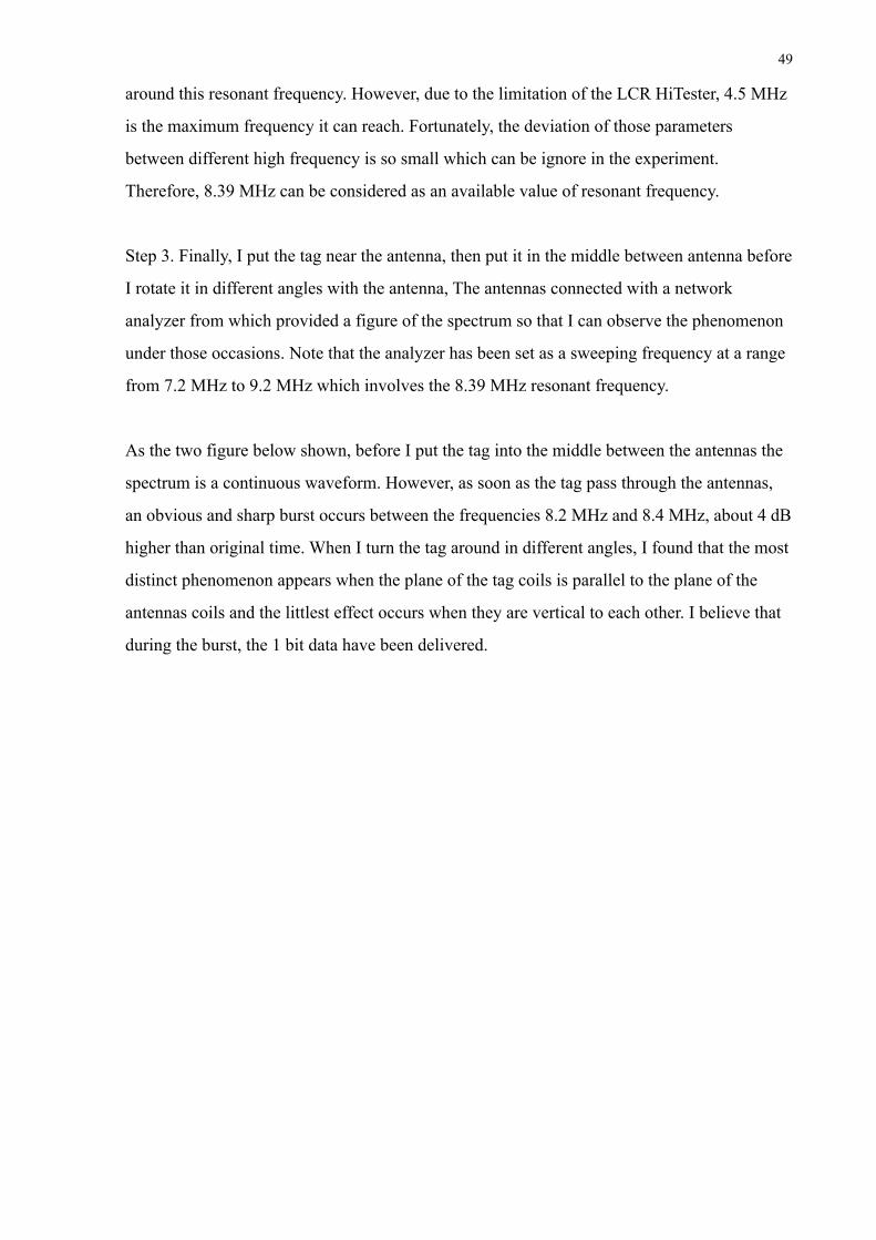
Step 3. Finally, I put the tag near the antenna, then put it in the middle between antenna before

I rotate it in different angles with the antenna, The antennas connected with a network

analyzer from which provided a figure of the spectrum so that I can observe the phenomenon

under those occasions. Note that the analyzer has been set as a sweeping frequency at a range

from 7.2 MHz to 9.2 MHz which involves the 8.39 MHz resonant frequency.

As the two figure below shown, before I put the tag into the middle between the antennas the

spectrum is a continuous waveform. However, as soon as the tag pass through the antennas,

an obvious and sharp burst occurs between the frequencies 8.2 MHz and 8.4 MHz, about 4 dB

higher than original time. When I turn the tag around in different angles, I found that the most

distinct phenomenon appears when the plane of the tag coils is parallel to the plane of the

antennas coils and the littlest effect occurs when they are vertical to each other. I believe that

during the burst, the 1 bit data have been delivered.

49

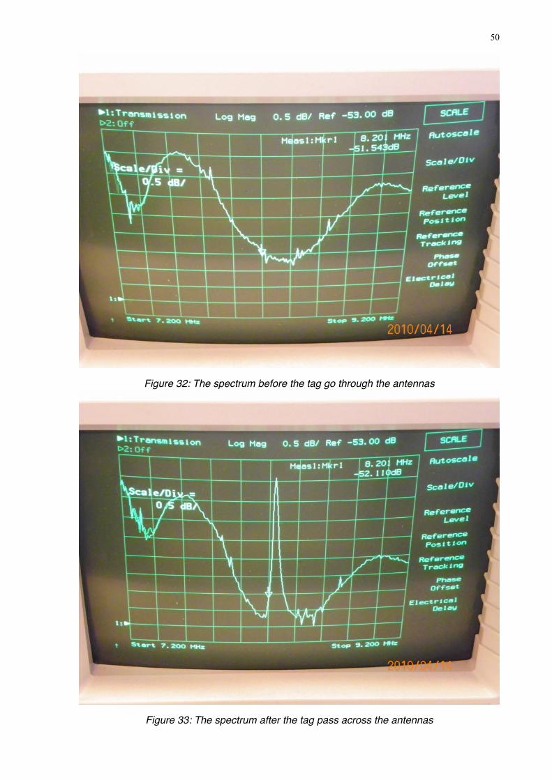
Figure 32: The spectrum before the tag go through the antennas

Figure 33: The spectrum after the tag pass across the antennas

50

4.1.5 Results

The above experiment demonstrated that 1 bit tag employs a resonant circuit to deliver the

data. The resonant frequency of the tag I used in this experiment is around 8.4 MHz. When

the tag goes through the antennas, there will be a distinct frequency response change at the

resonance frequency displayed on the network analyzer which is very likely to trigger an

alarm in the practice world.

4.2 UHF TAGS READING EXPERIMENT

4.2.1 Experiment purpose

In this experiment, I mainly focus on the test on reading two kinds of UHF tag through a

reader connected with a computer. In this section, I will try to answer the following questions:

What is the longest available distance that these two UHF tags can be detected by the reader?

What is the computer’s role in this communication? What else factors will affect the signal

issued from tags being discovered by reader except the distance? (like the locations of reader

and tags set or a different angle between them)

4.2.2 Equipment

Two different UHF tags in shape which is shown as the following figure.

51

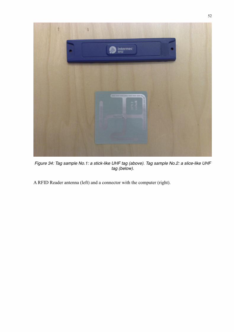
Figure 34: Tag sample No.1: a stick-like UHF tag (above). Tag sample No.2: a slice-like UHF tag (below).

A RFID Reader antenna (left) and a connector with the computer (right).

52

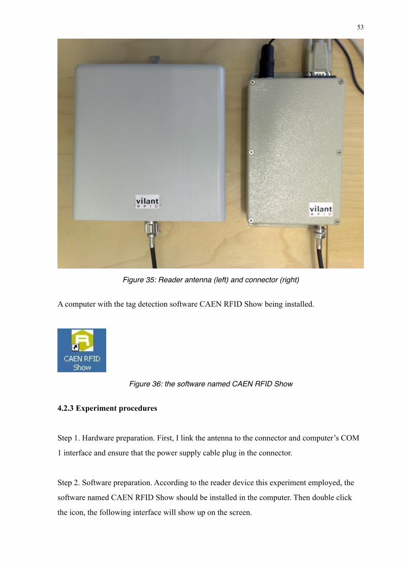
Figure 35: Reader antenna (left) and connector (right)

A computer with the tag detection software CAEN RFID Show being installed.

Figure 36: the software named CAEN RFID Show

4.2.3 Experiment procedures

Step 1. Hardware preparation. First, I link the antenna to the connector and computer’s COM

1 interface and ensure that the power supply cable plug in the connector.

Step 2. Software preparation. According to the reader device this experiment employed, the

software named CAEN RFID Show should be installed in the computer. Then double click

the icon, the following interface will show up on the screen.

53

Figure 37: operating interface of CAEN RFID Show

Click the settings and configuration the operating interface to the COM 1 which has already

connected to the reader. Then click Begin Acquisition button. If everything is correct, the

reader would start to detect the available tags in its reading range.

Step 3. Reading the tags. I first try the No. 1 tag. As soon as I put it in front of the antenna,

there is a response shown up in the software window. Additionally, we can see from the left-

hand corner of the software window; it also successfully recognize that this tag used an EPC

Class 1 Gen 2 protocol.

54

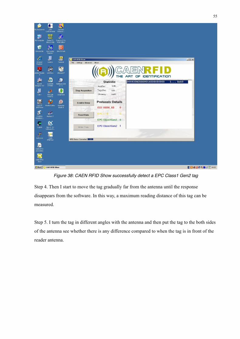
Figure 38: CAEN RFID Show successfully detect a EPC Class1 Gen2 tag

Step 4. Then I start to move the tag gradually far from the antenna until the response

disappears from the software. In this way, a maximum reading distance of this tag can be

measured.

Step 5. I turn the tag in different angles with the antenna and then put the tag to the both sides

of the antenna see whether there is any difference compared to when the tag is in front of the

reader antenna.

55

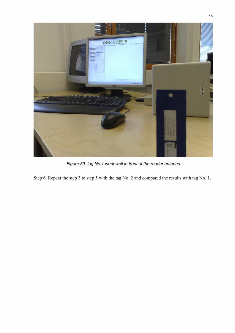
Figure 39: tag No.1 work well in front of the reader antenna

Step 6. Repeat the step 3 to step 5 with the tag No. 2 and compared the results with tag No. 1.

56

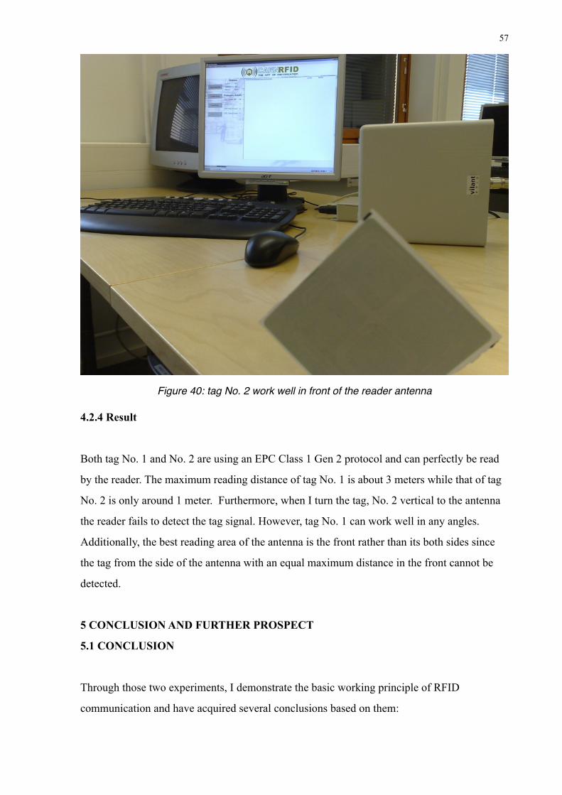
Figure 40: tag No. 2 work well in front of the reader antenna

4.2.4 Result

Both tag No. 1 and No. 2 are using an EPC Class 1 Gen 2 protocol and can perfectly be read

by the reader. The maximum reading distance of tag No. 1 is about 3 meters while that of tag

No. 2 is only around 1 meter. Furthermore, when I turn the tag, No. 2 vertical to the antenna

the reader fails to detect the tag signal. However, tag No. 1 can work well in any angles.

Additionally, the best reading area of the antenna is the front rather than its both sides since

the tag from the side of the antenna with an equal maximum distance in the front cannot be

detected.

5 CONCLUSION AND FURTHER PROSPECT

5.1 CONCLUSION

Through those two experiments, I demonstrate the basic working principle of RFID

communication and have acquired several conclusions based on them:

57

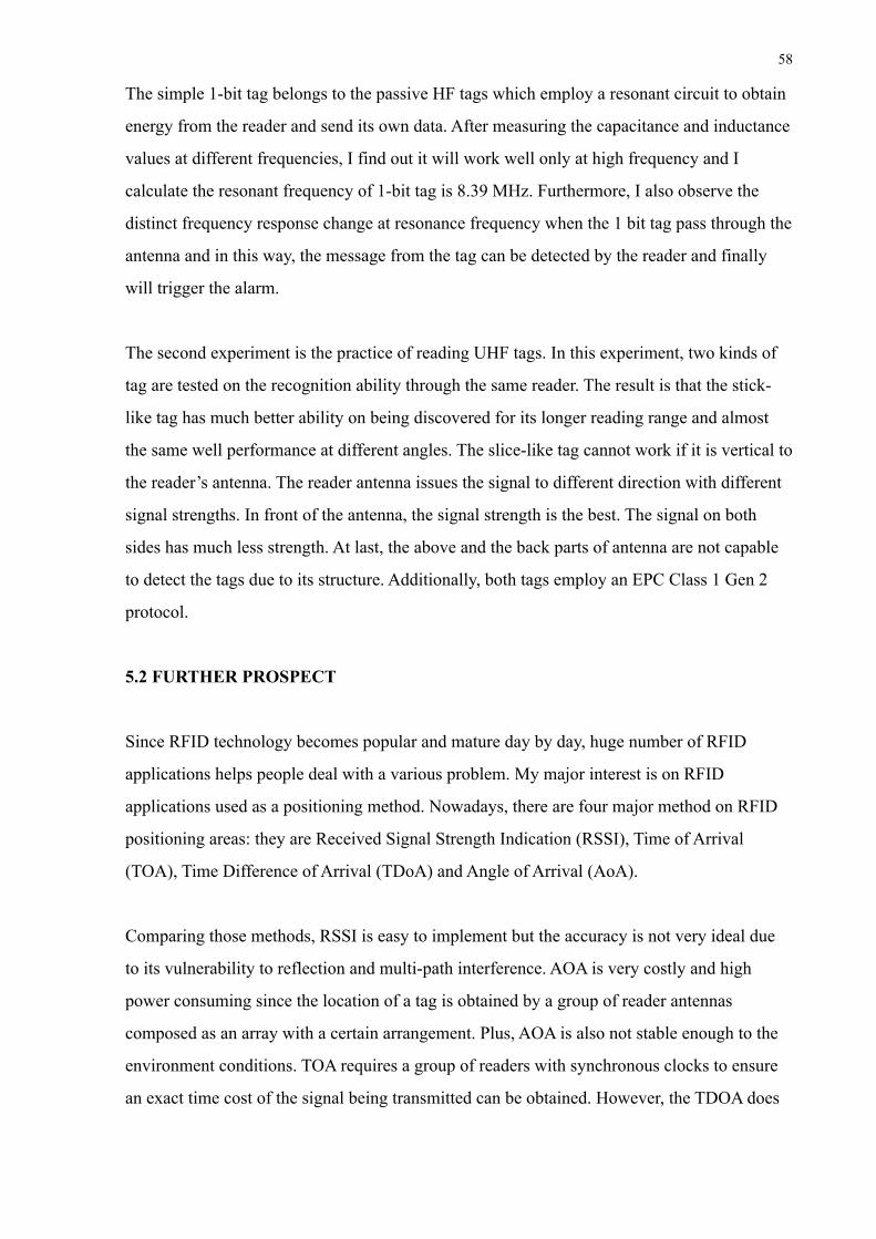
The simple 1-bit tag belongs to the passive HF tags which employ a resonant circuit to obtain

energy from the reader and send its own data. After measuring the capacitance and inductance

values at different frequencies, I find out it will work well only at high frequency and I

calculate the resonant frequency of 1-bit tag is 8.39 MHz. Furthermore, I also observe the

distinct frequency response change at resonance frequency when the 1 bit tag pass through the

antenna and in this way, the message from the tag can be detected by the reader and finally

will trigger the alarm.

The second experiment is the practice of reading UHF tags. In this experiment, two kinds of

tag are tested on the recognition ability through the same reader. The result is that the stick-

like tag has much better ability on being discovered for its longer reading range and almost

the same well performance at different angles. The slice-like tag cannot work if it is vertical to

the reader’s antenna. The reader antenna issues the signal to different direction with different

signal strengths. In front of the antenna, the signal strength is the best. The signal on both

sides has much less strength. At last, the above and the back parts of antenna are not capable

to detect the tags due to its structure. Additionally, both tags employ an EPC Class 1 Gen 2

protocol.

5.2 FURTHER PROSPECT

Since RFID technology becomes popular and mature day by day, huge number of RFID

applications helps people deal with a various problem. My major interest is on RFID

applications used as a positioning method. Nowadays, there are four major method on RFID

positioning areas: they are Received Signal Strength Indication (RSSI), Time of Arrival

(TOA), Time Difference of Arrival (TDoA) and Angle of Arrival (AoA).

Comparing those methods, RSSI is easy to implement but the accuracy is not very ideal due

to its vulnerability to reflection and multi-path interference. AOA is very costly and high

power consuming since the location of a tag is obtained by a group of reader antennas

composed as an array with a certain arrangement. Plus, AOA is also not stable enough to the

environment conditions. TOA requires a group of readers with synchronous clocks to ensure

an exact time cost of the signal being transmitted can be obtained. However, the TDOA does

58

not. Moreover, by improving TOA to TDOA, the ability of tolerance about objects reflection

is also promoted which stands for a higher accuracy.

In general speaking, nowadays, TDOA is a RFID positioning method with great potential in

the future development. However, it still has some limitations that need to be overcome, for

example, when facing with the narrow band signal (many RFID communicating signal use a

narrow-band transmission), the time resolution of the TDOA in a multipath environment is

limited to approximately 1/B where B is the bandwidth of the received signal. For instance, a

0.3 m accuracy, we need a 1 ns time resolution. However, this resolution required a 1 GHz

bandwidth which is not available in current RFID systems. (Kumar [referred 16.5.2010])

Unfortunately, due to the limitation of the experiment facilities and time, I did not have the

chance to do more experiments on the RFID experiment related to positioning. However, I

would like to do some further study in RFID positioning in the future, especially in how to

conquer those limitations of TDOA.

59

6 REFERENCE

Books

Dobkin, Daniel M. 2008. The RF in RFID: Passive UHF RFID in practice. the United States

of America. Newsnes.

Finkenzeller, Klause 2003. RFID Handbook: Fundamentals and Applications in Contactless

Smart Cards and Identification, Second Edition, Wiley.

Theses

Mathieu Bouet. RFID Tags: Positioning Principles and Localization Techniques. In proc. of

RFID localization schemes, 2008.

S.R.Praveen Kumar. Improved TDOA For CDMA By Error Pattern Detection and

Correction. In proc. of Advantages for TDOA in CDMA, 1996.

Electronic sources

Radio-frequency identification. Available in www-format:

<URL: http://en.wikipedia.org/wiki/RFID>

Optical axis. Available in www-format:

<URL: http://en.wikipedia.org/wiki/Optical_axis>

Antenna boresight. Available in www-format:

<URL: http://en.wikipedia.org/wiki/Antenna_boresight>

60

http://en.wikipedia.org/wiki/RFID

http://en.wikipedia.org/wiki/RFID

http://en.wikipedia.org/wiki/Optical_axis

http://en.wikipedia.org/wiki/Optical_axis

http://en.wikipedia.org/wiki/Antenna_boresight

http://en.wikipedia.org/wiki/Antenna_boresight

Received signal strength indication. Available in www-format:

<URL: http://en.wikipedia.org/wiki/Received_Signal_Strength_Indication>

Time of arrival. Available in www-format:

<URL: http://en.wikipedia.org/wiki/Time_of_arrival>

Angle of arrival. Available in www-format:

<URL: http://en.wikipedia.org/wiki/Angle_of_arrival>

Frequency modulation. Available in www-format:

<URL: http://en.wikipedia.org/wiki/Frequency_modulation>

Multilateration. Available in www-format:

<URL: http://en.wikipedia.org/wiki/Time_difference_of_arrival>

RFID Basics: Backscatter Radio Links and Link Budgets. Available in www-format:

<URL: http://www.rfdesignline.com/howto/202200135>

Line code. Available in www-format:

<URL: http://en.wikipedia.org/wiki/Line_code>

Phase-shift keying. Available in www-format:

<URL: http://en.wikipedia.org/wiki/Phase-shift_keying>

Frequency-shift keying. Available in www-format:

<URL: http://en.wikipedia.org/wiki/Frequency-shift_keying>

Amplitude-shift keying. Available in www-format:

<URL: http://en.wikipedia.org/wiki/Amplitude-shift_keying>

On-off keying. Available in www-format:

<URL: http://en.wikipedia.org/wiki/On-off_keying>

61

http://en.wikipedia.org/wiki/Received_Signal_Strength_Indication

http://en.wikipedia.org/wiki/Received_Signal_Strength_Indication

http://en.wikipedia.org/wiki/Time_of_arrival

http://en.wikipedia.org/wiki/Time_of_arrival

http://en.wikipedia.org/wiki/Angle_of_arrival

http://en.wikipedia.org/wiki/Angle_of_arrival

http://en.wikipedia.org/wiki/Frequency_modulation

http://en.wikipedia.org/wiki/Frequency_modulation

http://en.wikipedia.org/wiki/Time_difference_of_arrival

http://en.wikipedia.org/wiki/Time_difference_of_arrival

http://www.rfdesignline.com/howto/202200135

http://www.rfdesignline.com/howto/202200135

http://en.wikipedia.org/wiki/Line_code

http://en.wikipedia.org/wiki/Line_code

http://en.wikipedia.org/wiki/Phase-shift_keying

http://en.wikipedia.org/wiki/Phase-shift_keying

http://en.wikipedia.org/wiki/Frequency-shift_keying

http://en.wikipedia.org/wiki/Frequency-shift_keying

http://en.wikipedia.org/wiki/Amplitude-shift_keying

http://en.wikipedia.org/wiki/Amplitude-shift_keying

http://en.wikipedia.org/wiki/On-off_keying

http://en.wikipedia.org/wiki/On-off_keying

Continuous wave. Available in www-format:

<URL: http://en.wikipedia.org/wiki/Continuous_wave>

Carrier wave. Available in www-format:

<URL: http://en.wikipedia.org/wiki/Carrier_wave>

Electromagnetic radiation. Available in www-format:

<URL: http://en.wikipedia.org/wiki/Electromagnetic_radiation>

62

http://en.wikipedia.org/wiki/Continuous_wave

http://en.wikipedia.org/wiki/Continuous_wave

http://en.wikipedia.org/wiki/Carrier_wave

http://en.wikipedia.org/wiki/Carrier_wave

http://en.wikipedia.org/wiki/Electromagnetic_radiation

http://en.wikipedia.org/wiki/Electromagnetic_radiation

Documents

Tang Zimu RFID Systems and Applications in Positioning