Embed Size (px)
Citation preview
Talking Trends
Macroeconomics and Markets
March 2016
No. 5
The views expressed in the Bulletin
are solely those of the authors and do not necessarily reflect the official position of the Bank of Russia.
Please send your comments and suggestions on the content at [email protected]
Research and
Forecasting
Department Bulletin
Серия до кла до в о б э ко но мичеСких
иССледо ва ниях 2 No. 5 / March 2016
Macroeconomics and markets No. 1 / October
2015
Talking Trends
CONTENTS
Executive summary ____________________________________________________ 3
1. Monthly summary ___________________________________________________ 4
1.1. The current drop in inflation is largely explained by the temporary factors
coming into play, with the risks inflation may move away from target _________ 4
1.1.1. The slowdown in food inflation is caused by a few factors beyond demand
constraints ______________________________________________________________ 4 1.1.2. The implications of monetary factors, global food prices and exchange rate for
inflation in Russia _______________________________________________________ 11 1.1.3. Inflation expectations in March: the drop has not been persistent ______________ 14 1.1.4. Underlying inflation is continuing to recede slowly __________________________ 15 1.1.5. Balance of payments: high ruble exchange rate sensitivity to external shocks
comes laden with inflation risks _____________________________________________ 17
1.2. The structural shifts currently underway in the Russian economy helped
cushion the slump but have so far failed to put it back on a growth path _____ 17
1.2.1. Industrial production in February: the impact of the weather and calendar factors
complicates current situation assessments ____________________________________ 17 1.2.2. Structural shifts in manufacturing are tilted towards intermediate demand industries 22 1.2.3. The rising output in key industries in February should not be overinterpreted _____ 26 1.2.4. March PMI survey, production: growth is on hold___________________________ 29 1.2.5. Unemployment remains stable ________________________________________ 30 1.2.6. Russian producers remain competitive over their Chinese counterparts on the back
of a stronger yuan _______________________________________________________ 31
1.3. Global economy, financial and commodity markets ___________________ 34
1.3.1. The soft stance of major central banks helps check global economic slowdown
risks__________________________________________________________________ 34 1.3.2. Financial markets: the decline in volatility may prove temporary _______________ 39 1.3.3. Commodity markets: rally and reversal in the end of the month ________________ 43
2. Outlook: leading indicators ___________________________________________ 48
2.1. Global leading indicators _________________________________________ 48
2.1.1. The economic rebound in the emerging nations could prove short-term _________ 48
2.2. What do Russian leading indicators suggest? ________________________ 50
2.2.1. Short-term index GDP assessment: the February data match our expectations ___ 50 2.2.2. Leading business indicator: mixed signals ________________________________ 54 2.2.3. Financial analysts' forecasts __________________________________________ 55
3. In focus ___________________________________________________________ 57
The impact of informal employment on GDP and inflation ________________________ 57
Серия до кла до в о б э ко но мичеСких
иССледо ва ниях 3 No. 5 / March 2016
Macroeconomics and markets No. 1 / October
2015
Talking Trends
Executive summary
1. Monthly summary
In March, price growth continued to slow, the economy balanced between reces-
sion and stagnation, risks to stability of the Russian financial markets went down.
o Inflationary pressure in March eased stronger than expected, driven by mone-
tary policy. Ruble appreciation and the impact of temporary favourable factors in
the food market made a positive contribution to decrease in inflation. However,
risks of inflation exceeding the 4% target in 2017 are still high due to persis-
tent uncertainty surrounding the fiscal policy, slow decline in inflation expecta-
tions and possible termination of temporary favourable factors.
o The production dynamics signal higher stability of the economy to negative oil
price shocks. The risks of a new spiral of recession failed to materialise. Individ-
ual sectors and industries show structural shifts towards the tradables sector, as
well as higher output.
o Although the BoR key rate has been kept on hold, monetary conditions are
continuing to ease following the gradual shift from structural liquidity deficit to
surplus.
2. Outlook
The soft stance of major central banks’ monetary policy suggests that the threat of
a slowdown of the global economic growth has reduced. However, medium-term
risks remain high as the prospects of effective transformation of the Chinese
economy are still uncertain.
Russian leading business indicators suggest that sustainable economic growth re-
covery is not very likely in the months to come, through the economy is picking up
after the winter drop in oil prices.
3. In focus: The impact of informal employment on GDP and inflation
The informal employment phenomenon curbs unemployment growth in this time of
crisis...
...but the persistently sustainable growth of informal employment may aggravate
structural problems in the labour market and trigger additional inflation risks in the
medium term.
Серия до кла до в о б э ко но мичеСких
иССледо ва ниях 4 No. 5 / March 2016
Macroeconomics and markets No. 1 / October
2015
Talking Trends
1. Monthly summary
1.1. The current drop in inflation is largely explained by the temporary
factors coming into play, with the risks inflation may move away from target
Inflationary pressure in March abated more than expected, driven by the monetary
policy. Support came from a stronger ruble, together with the arrival of temporary favour-
able drivers in the food market. However, the risks that inflation may exceed the 4% tar-
get in 2017 are still high; these stem from the uncertainty over the fiscal policy, slowly de-
clining inflation expectations and the probable cessation of the impact from the temporary
favourable factors.
1.1.1. The slowdown in food inflation is caused by a few factors beyond
demand constraints
Food products are known for weaker demand elasticity compared to non-food,
which makes it impossible to attribute slowly rising food prices to weak demand
only.
Growth of food prices is checked by several factors on the supply side (globally
declining food prices, last year's rich harvest and abundant production of several
products). Some of these drivers are temporary in nature.
The strong slowdown in seasonally adjusted growth on fruit and vegetables in H1
could well be succeeded by a more significant than usual price acceleration in H2.
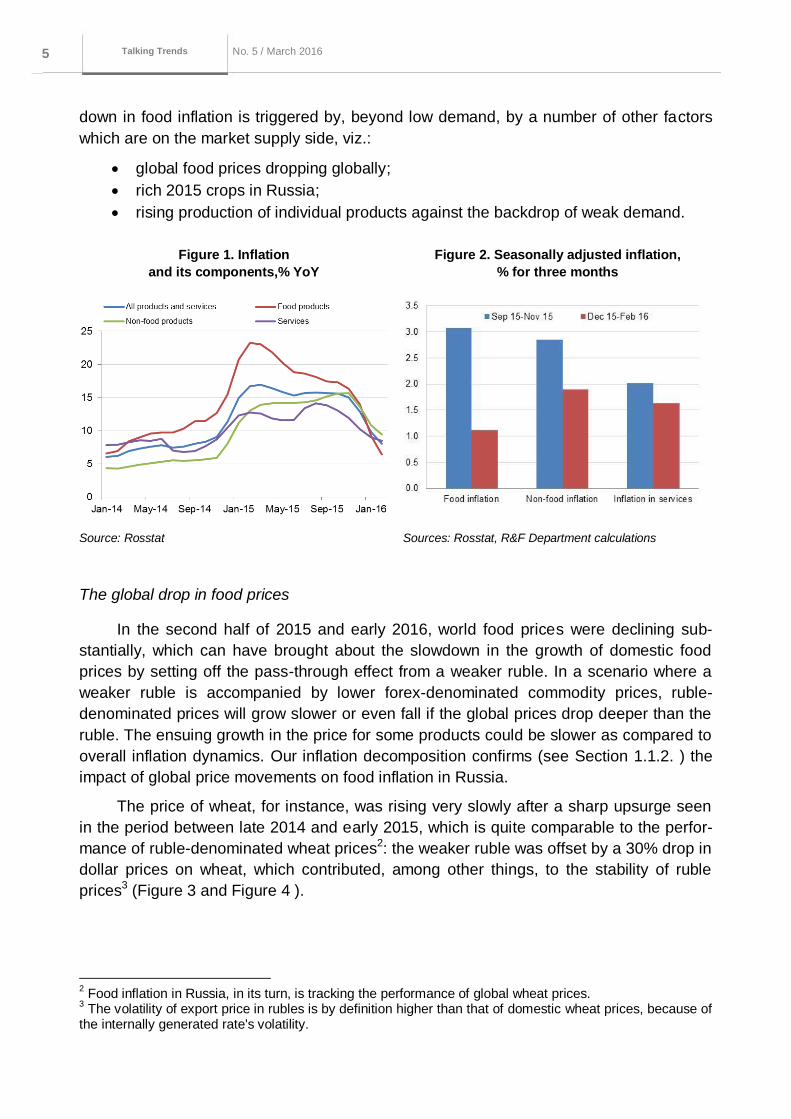
Annual inflation showed a notable slowdown in the last few months, which may be
explained, to a large extent, by the high base of the past year. Annualised rates of food
price growth, much to our surprise, showed a strong slowdown: in February and March
these were lower than those for non-food products and services (Figure 1). A proper ex-
planation to this could be the withdrawal from annual inflation estimation of the high rates
of price growth seen in the start of the past year1. However, as we look into seasonally
adjusted price dynamics of the three key consumer price index (CPI) components, we
could point to other factors which are behind the slowdown in food product prices, beyond
the high base effect (Figure 2).
The strongly slowed nominal income could have come about as a result of weaker
overall pressure caused by, inter alia, minor pension and salary indexation in the public
sector. Theoretically though, this could make itself more evident in non-food, rather than
food, prices, with the known smaller price elasticity of the latter. Our view is that the slow-
1 Food inflation was much stronger than that for non-food products and services, hence, all other things
being equal, a symmetric drop in inflation could be envisaged in one year's time.
Серия до кла до в о б э ко но мичеСких
иССледо ва ниях 5 No. 5 / March 2016
Macroeconomics and markets No. 1 / October
2015
Talking Trends
down in food inflation is triggered by, beyond low demand, by a number of other factors
which are on the market supply side, viz.:
global food prices dropping globally;
rich 2015 crops in Russia;
rising production of individual products against the backdrop of weak demand.
Figure 1. Inflation
and its components,% YoY
Figure 2. Seasonally adjusted inflation,
% for three months
Source: Rosstat Sources: Rosstat, R&F Department calculations
The global drop in food prices
In the second half of 2015 and early 2016, world food prices were declining sub-
stantially, which can have brought about the slowdown in the growth of domestic food
prices by setting off the pass-through effect from a weaker ruble. In a scenario where a
weaker ruble is accompanied by lower forex-denominated commodity prices, ruble-
denominated prices will grow slower or even fall if the global prices drop deeper than the
ruble. The ensuing growth in the price for some products could be slower as compared to
overall inflation dynamics. Our inflation decomposition confirms (see Section 1.1.2. ) the
impact of global price movements on food inflation in Russia.
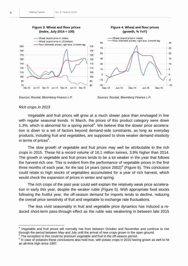
The price of wheat, for instance, was rising very slowly after a sharp upsurge seen
in the period between late 2014 and early 2015, which is quite comparable to the perfor-
mance of ruble-denominated wheat prices2: the weaker ruble was offset by a 30% drop in
dollar prices on wheat, which contributed, among other things, to the stability of ruble
prices3 (Figure 3 and Figure 4 ).
2 Food inflation in Russia, in its turn, is tracking the performance of global wheat prices.
3 The volatility of export price in rubles is by definition higher than that of domestic wheat prices, because of
the internally generated rate's volatility.
Серия до кла до в о б э ко но мичеСких
иССледо ва ниях 6 No. 5 / March 2016
Macroeconomics and markets No. 1 / October
2015
Talking Trends
Figure 3. Wheat and flour prices
(index, July 2014 = 100)
Figure 4. Wheat and flour prices
(growth, % YoY)
Sources: Rosstat, Bloomberg Finance L.P. Sources: Rosstat, Bloomberg Finance L.P.
Rich crops in 2015
Vegetable and fruit prices will grow at a much slower pace than envisaged in line
with regular seasonal trends. In March, the prices of this product category were down
1.3%, which is abnormal for a spring period4. We believe that the slower price accelera-
tion is down to a set of factors beyond demand-side constraints, as long as everyday
products, including fruit and vegetables, are supposed to show weaker demand elasticity
in terms of prices5.
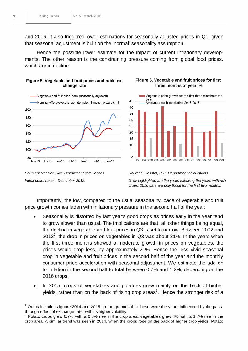
The slow growth of vegetable and fruit prices may well be attributable to the rich
crops in 2015. These hit a record volume of 16.1 million tonnes, 3.9% higher than 2014.
The growth in vegetable and fruit prices tends to be a lot weaker in the year that follows
the harvest-rich one. This is evident from the performance of vegetable prices in the first
three months of each year, for the last 14 years (since 2002)6 (Figure 6). This conclusion
could relate to high stocks of vegetables accumulated for a year of rich harvest, which
would check the expansion of prices in winter and spring.
The rich crops of the past year could well explain the relatively weak price accelera-
tion in early this year, despite the weaker ruble (Figure 5). With appropriate food stocks
following the fruitful year, the off-season demand for imports tends to decline, reducing
the overall price sensitivity of fruit and vegetable to exchange rate fluctuations.
The less vivid seasonality in fruit and vegetable price dynamics has induced a re-
duced short-term pass-through effect as the ruble was weakening in between late 2015
4 Vegetable and fruit prices will normally rise from between October and November and continue to rise
through the period between May and July until the arrival of new crops grown in the open ground. 5 The exception to this could be premium vegetable and fruit in the off-season period.
6 In case of potatoes these conclusions also hold true, with potato crops in 2015 having grown as well to hit
an all-time high since 1997.
Серия до кла до в о б э ко но мичеСких
иССледо ва ниях 7 No. 5 / March 2016
Macroeconomics and markets No. 1 / October
2015
Talking Trends
and 2016. It also triggered lower estimations for seasonally adjusted prices in Q1, given
that seasonal adjustment is built on the 'normal' seasonality assumption.
Hence the possible lower estimate for the impact of current inflationary develop-
ments. The other reason is the constraining pressure coming from global food prices,
which are in decline.
Figure 5. Vegetable and fruit prices and ruble ex-change rate
Figure 6. Vegetable and fruit prices for first
three months of year, %
Sources: Rosstat, R&F Department calculations
Index count base – December 2012.
Sources: Rosstat, R&F Department calculations
Grey-highlighted are the years following the years with rich
crops; 2016 data are only those for the first two months.
Importantly, the low, compared to the usual seasonality, pace of vegetable and fruit
price growth comes laden with inflationary pressure in the second half of the year:
Seasonality is distorted by last year's good crops as prices early in the year tend
to grow slower than usual. The implications are that, all other things being equal,
the decline in vegetable and fruit prices in Q3 is set to narrow. Between 2002 and
20137, the drop in prices on vegetables in Q3 was about 31%. In the years when
the first three months showed a moderate growth in prices on vegetables, the
prices would drop less, by approximately 21%. Hence the less vivid seasonal
drop in vegetable and fruit prices in the second half of the year and the monthly
consumer price acceleration with seasonal adjustment. We estimate the add-on
to inflation in the second half to total between 0.7% and 1.2%, depending on the
2016 crops.
In 2015, crops of vegetables and potatoes grew mainly on the back of higher
yields, rather than on the back of rising crop areas8. Hence the stronger risk of a
7 Our calculations ignore 2014 and 2015 on the grounds that these were the years influenced by the pass-
through effect of exchange rate, with its higher volatility. 8 Potato crops grew 6.7% with a 0.8% rise in the crop area; vegetables grew 4% with a 1.7% rise in the
crop area. A similar trend was seen in 2014, when the crops rose on the back of higher crop yields. Potato
Серия до кла до в о б э ко но мичеСких
иССледо ва ниях 8 No. 5 / March 2016
Macroeconomics and markets No. 1 / October
2015
Talking Trends
minor price contraction in the second half of the year (provided that this year's
yields are lower than in 2015 and the crop areas remain essentially level).
Growing production of individual products against weak demand
The implications of demand constraints are not to be viewed separately from the
developments in one product category or another. Amid a slowing or dropping demand,
the impact on prices could vary depending on supply developments. For instance, if the
supply of goods is dropping faster than its demand, its price could grow; while supply
growing on the backdrop of weaker demand could cause the price to drop substantially.
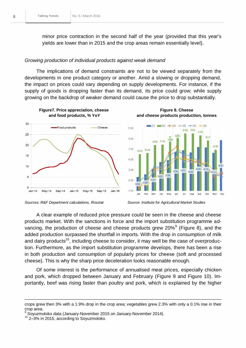
Figure7. Price appreciation, cheese
and food products, % YoY
Figure 8. Cheese
and cheese products production, tonnes
Sources: R&F Department calculations, Rosstat Source: Institute for Agricultural Market Studies
A clear example of reduced price pressure could be seen in the cheese and cheese
products market. With the sanctions in force and the import substitution programme ad-
vancing, the production of cheese and cheese products grew 20%9 (Figure 8), and the
added production surpassed the shortfall in imports. With the drop in consumption of milk
and dairy products10, including cheese to consider, it may well be the case of overproduc-
tion. Furthermore, as the import substitution programme develops, there has been a rise
in both production and consumption of popularly prices for cheese (soft and processed
cheese). This is why the sharp price deceleration looks reasonable enough.
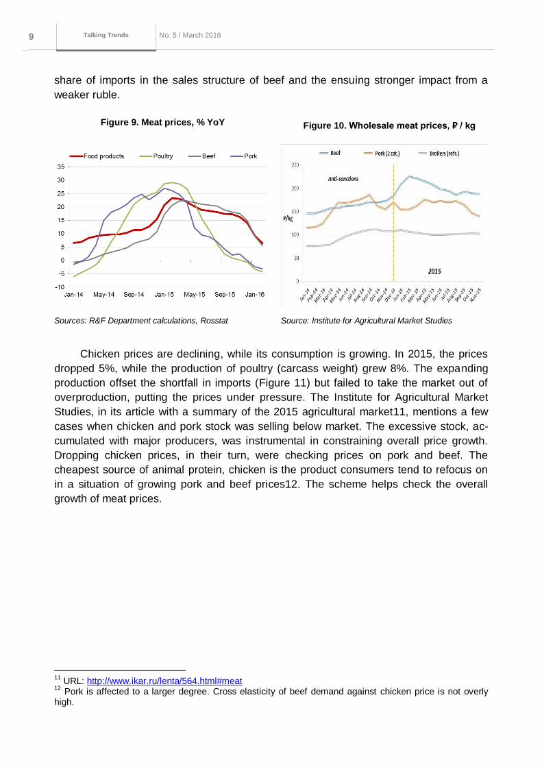
Of some interest is the performance of annualised meat prices, especially chicken
and pork, which dropped between January and February (Figure 9 and Figure 10). Im-
portantly, beef was rising faster than poultry and pork, which is explained by the higher
crops grew then 3% with a 1.9% drop in the crop area; vegetables grew 2.3% with only a 0.1% rise in their crop area. 9 Soyuzmoloko data (January-November 2015 on January-November 2014).
10 2–3% in 2015, according to Soyuzmoloko.
Серия до кла до в о б э ко но мичеСких
иССледо ва ниях 9 No. 5 / March 2016
Macroeconomics and markets No. 1 / October
2015
Talking Trends
share of imports in the sales structure of beef and the ensuing stronger impact from a
weaker ruble.
Figure 9. Meat prices, % YoY Figure 10. Wholesale meat prices, ₽ / kg
Sources: R&F Department calculations, Rosstat Source: Institute for Agricultural Market Studies
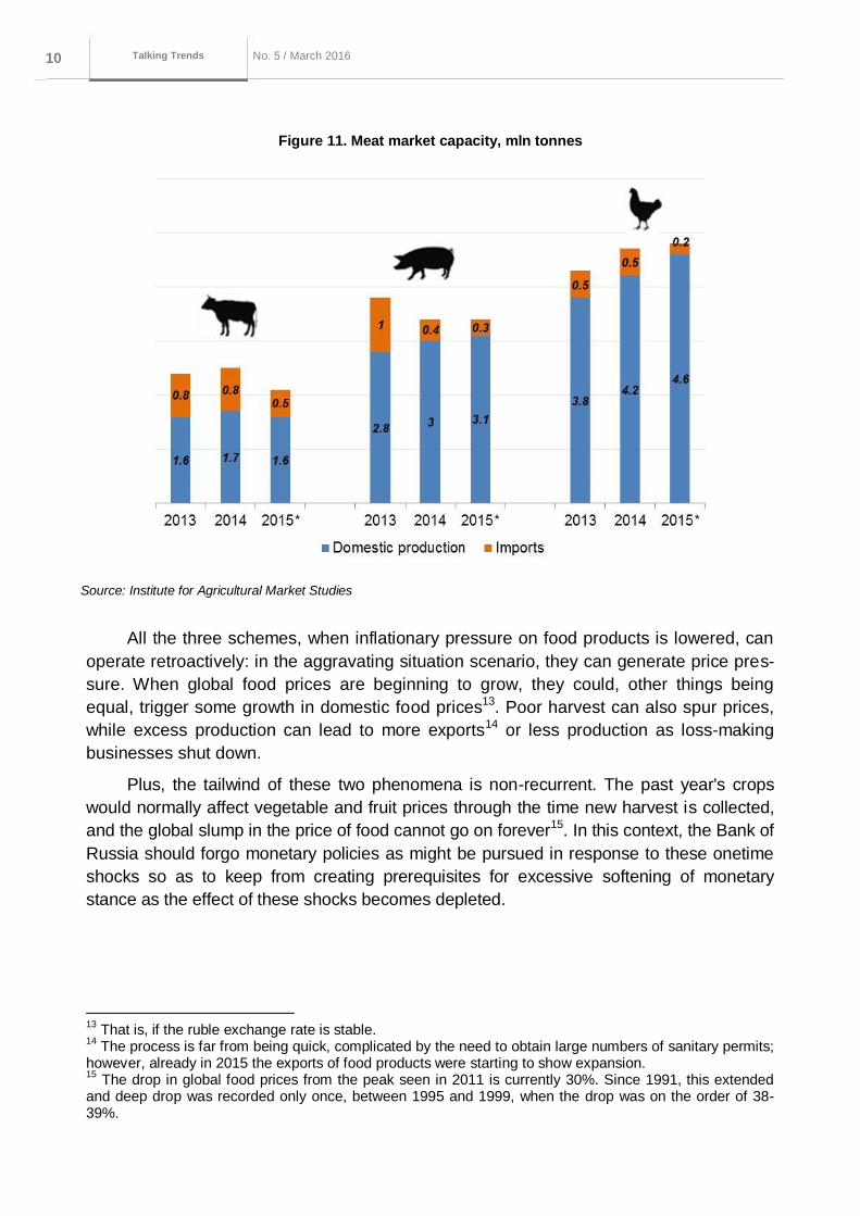
Chicken prices are declining, while its consumption is growing. In 2015, the prices
dropped 5%, while the production of poultry (carcass weight) grew 8%. The expanding
production offset the shortfall in imports (Figure 11) but failed to take the market out of
overproduction, putting the prices under pressure. The Institute for Agricultural Market
Studies, in its article with a summary of the 2015 agricultural market11, mentions a few
cases when chicken and pork stock was selling below market. The excessive stock, ac-
cumulated with major producers, was instrumental in constraining overall price growth.
Dropping chicken prices, in their turn, were checking prices on pork and beef. The
cheapest source of animal protein, chicken is the product consumers tend to refocus on
in a situation of growing pork and beef prices12. The scheme helps check the overall
growth of meat prices.
11
URL: http://www.ikar.ru/lenta/564.html#meat 12
Pork is affected to a larger degree. Cross elasticity of beef demand against chicken price is not overly high.
Серия до кла до в о б э ко но мичеСких
иССледо ва ниях 10 No. 5 / March 2016
Macroeconomics and markets No. 1 / October
2015
Talking Trends
Figure 11. Meat market capacity, mln tonnes
Source: Institute for Agricultural Market Studies
All the three schemes, when inflationary pressure on food products is lowered, can
operate retroactively: in the aggravating situation scenario, they can generate price pres-
sure. When global food prices are beginning to grow, they could, other things being
equal, trigger some growth in domestic food prices13. Poor harvest can also spur prices,
while excess production can lead to more exports14 or less production as loss-making
businesses shut down.
Plus, the tailwind of these two phenomena is non-recurrent. The past year's crops
would normally affect vegetable and fruit prices through the time new harvest is collected,
and the global slump in the price of food cannot go on forever15. In this context, the Bank of
Russia should forgo monetary policies as might be pursued in response to these onetime
shocks so as to keep from creating prerequisites for excessive softening of monetary
stance as the effect of these shocks becomes depleted.
13
That is, if the ruble exchange rate is stable. 14
The process is far from being quick, complicated by the need to obtain large numbers of sanitary permits; however, already in 2015 the exports of food products were starting to show expansion. 15
The drop in global food prices from the peak seen in 2011 is currently 30%. Since 1991, this extended and deep drop was recorded only once, between 1995 and 1999, when the drop was on the order of 38-39%.
Серия до кла до в о б э ко но мичеСких
иССледо ва ниях 11 No. 5 / March 2016
Macroeconomics and markets No. 1 / October
2015
Talking Trends
1.1.2. The implications of monetary factors, global food prices
and exchange rate for inflation in Russia
Monetary factors are the key contributor to inflation, although their importance was
growing somewhat weaker over the last year, and their contribution to inflation was
well below the values seen between 2006 and 2008.
The global food prices, declining since mid-2014, served as a certain deterrent for
2015 prices.
A change in external conditions comes laden with the risks of emerging inflationary
shocks, either negative or positive.
Unless broken down by separate components, the picture of price acceleration is
not informative enough. The decomposition of inflation enabled us to gain a deep insight
into which components are responsible for its performance. The conditional monetary
component and non-monetary inflation components were established. The factors con-
sidered as non-monetary components included the currency exchange rate, railroad
rates, utility prices and the global agricultural product prices16.
R&F Department inflation decomposition methodology
According to the methodology, inflation was broken down into four components: monetary infla-tion, the exchange rate, food prices and other
17. The latter component is made up of any unaccount-
ed-for factors which are impactful on inflation, albeit with very minor effect, or such which could hardly be quantified at all (e.g., the impact on inflation from the demand side). The decomposition was based on monthly data for the period between 2006 through 2016. The econometric model used the new in-flation seasonal adjustment
18, with the relative data available since 2006, which was behind the deci-
sion on the period for the assessment.
'Monetary' inflation was computed through singling out the common low frequency component in the performance of several indicators, representative of nominal processes in the economy. We pro-ceed from the assumption that this component is unexposed to specific shocks which are not common to all indicators or to short-term fluctuations which can be neglected for the monetary policy purposes. The calculations are based on the dynamic factor model. As nominal indicators, the CPI and seven other indicators were used, the majority of them being common domestically generated inflation indi-cators: prices of services, housing prices, fixed capital investment deflator, GDP deflator, unit labour costs, M2Y monetary aggregate, and the ruble nominal effective exchange rate. The calculations used monthly seasonally adjusted (interpolated if necessary) growth rates. The same method was applied to calculate the monetary component in the exchange rate performance.
Thereafter we looked into the effect of other factors on the non-monetary inflation component, as is the result of the monetary component subtracted from the actual inflation. The exchange rate performance was also adjusted for the previously computed monetary component. This was followed by a simple regression equation to quantify the impact of exchange rate and global food prices on the
non-monetary inflation. The unaccounted-for performance was classed as 'Other' (Figure 12).
16
We assume global food prices to impact on domestic prices as long as much of food products consumed in Russia are exports. 17
The analysis found the government-regulated rates to exert only minor pressure on inflation, which is why these components were withdrawn from the analysis and classed as 'Other' in our model. 18
For details of the methodology see 'Talking Trends' No. 4, February 2016, Section 3 'In focus. The seasonal adjustment in consumer inflation problem’.

Серия до кла до в о б э ко но мичеСких
иССледо ва ниях 12 No. 5 / March 2016
Macroeconomics and markets No. 1 / October
2015
Talking Trends
The calculations showed (Figure 12) that the exchange rate pass-through effect
weighs on prices for half a year. Most of the exchange rate pass-through effect falls on
the first three months and totals circa 0.13, with the aggregate effect of 0.1919. Global
food price changes also put pressure on inflation, remaining in effect for four consecutive
months. Their aggregate effect proved equal to 0.03.
Figure 12. Inflation decomposition, % YoY
Source: R&F Department calculations
Monetary inflation accounts for most of overall inflation. Importantly, it was some-
what down over the course of the last year, while it is appreciably less than seen in 2006-
2008. As suggested by this decomposition, all price acceleration seen between late 2014
and early 2015 was essentially down to the ruble weakening. The impact of this effect on
annual inflation recedes as this price upsurge gradually quits the basis for calculation.
The drop in global food prices since mid-201420 was putting some downward pressure on
prices in 2015 (with a contribution of circa -0.5 pp).
The results of these calculations should be treated very carefully. One of the draw-
backs of the decomposition as presented would be the assumption that the exchange
rate pass-through effect is constant in time. However, this effect is more flexible and will
at time change both in scale and in specific economic activity. For instance, the growth of
prices with a high export component in early 2016 was a lot more modest than early last 19
The pass-through effect of 0.19 means that a 1% weakening / strengthening in the exchange rate, other things being equal, will result in a 0.19 pp acceleration (slowdown) of inflation. 20
The IMF-calculated global food price index is down 27% in the period between April 2014 and February 2016.
Серия до кла до в о б э ко но мичеСких
иССледо ва ниях 13 No. 5 / March 2016
Macroeconomics and markets No. 1 / October
2015
Talking Trends
year. This is caused by, inter alia, a fading exchange rate pass-through effect. As regards
the decomposition as presented, this aspect is expressed in the arrival of negative contri-
bution from 'Other factors' over the last 2-3 months.
These drawbacks notwithstanding, the decomposition model as described enables
to see that changing external conditions could induce sufficiently strong inflationary
shocks in either side.
Regarding the current exchange rate pass-through effect on prices
There are a few explanations as to why the exchange rate pass-through effect seems weaker
than one year ago. According to one of these, sellers knowingly refrain from imputing the growing
costs, as relate to a weaker ruble, to consumer prices, so as to counter, among other things, weak
demand and retain market share. Manufacturers and resellers have to sacrifice some of their margin
which, in some cases, could be zero or even negative. This approach is affordable for major interna-
tional corporations, as Russia in their sales structure is but a small part. Therefore, they can carry on
operations notwithstanding this temporary drop in margin. However, this situation cannot linger on,
and with the onset of sustainable recovery in consumer demand suppliers will raise selling prices even
with costs unchanged so as to restore the margins to an appropriate level. This is another risk for ac-
celerated inflation in the second half of this or next year.
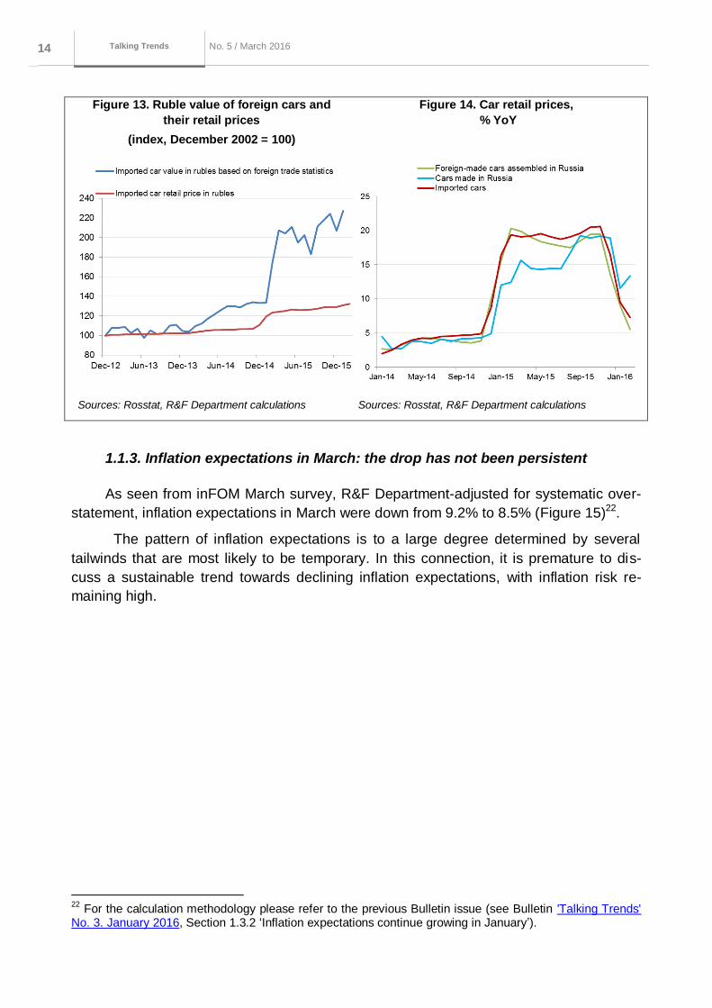
The above explanation is supported by developments in the car market, in particular, the market
of imported cars. We calculated the cost of Russia-bound cars in rubles and compared consumer
prices on foreign brands (Figure 13). The resulting average dollar price of imported cars in 2015 was
practically unchanged against 2014 (circa $18,500). It goes to show that the ruble value of a foreign
car has since the start of 2014 risen almost 120%21
, while retail prices rose only 28%. This implies that
importers' (and manufacturers') margins have dropped substantially and may have become negative.
This is indirectly evidenced by annualised price acceleration across various car classes. De-
spite the strong ruble weakening of late 2015 - early 2016, prices on foreign cars were growing slower
than domestically manufactured (Figure 14). No Russian manufacturer can currently boast any safety
margin to hold prices as long as they have been operating at a loss. Russian manufacturers have a
long way to go to reach a 100% localisation, which makes them shift the burden of growing costs of
component parts to retail prices.
21
As of January 2016.
Серия до кла до в о б э ко но мичеСких
иССледо ва ниях 14 No. 5 / March 2016
Macroeconomics and markets No. 1 / October
2015
Talking Trends
Figure 13. Ruble value of foreign cars and
their retail prices
(index, December 2002 = 100)
Figure 14. Car retail prices,
% YoY
Sources: Rosstat, R&F Department calculations Sources: Rosstat, R&F Department calculations
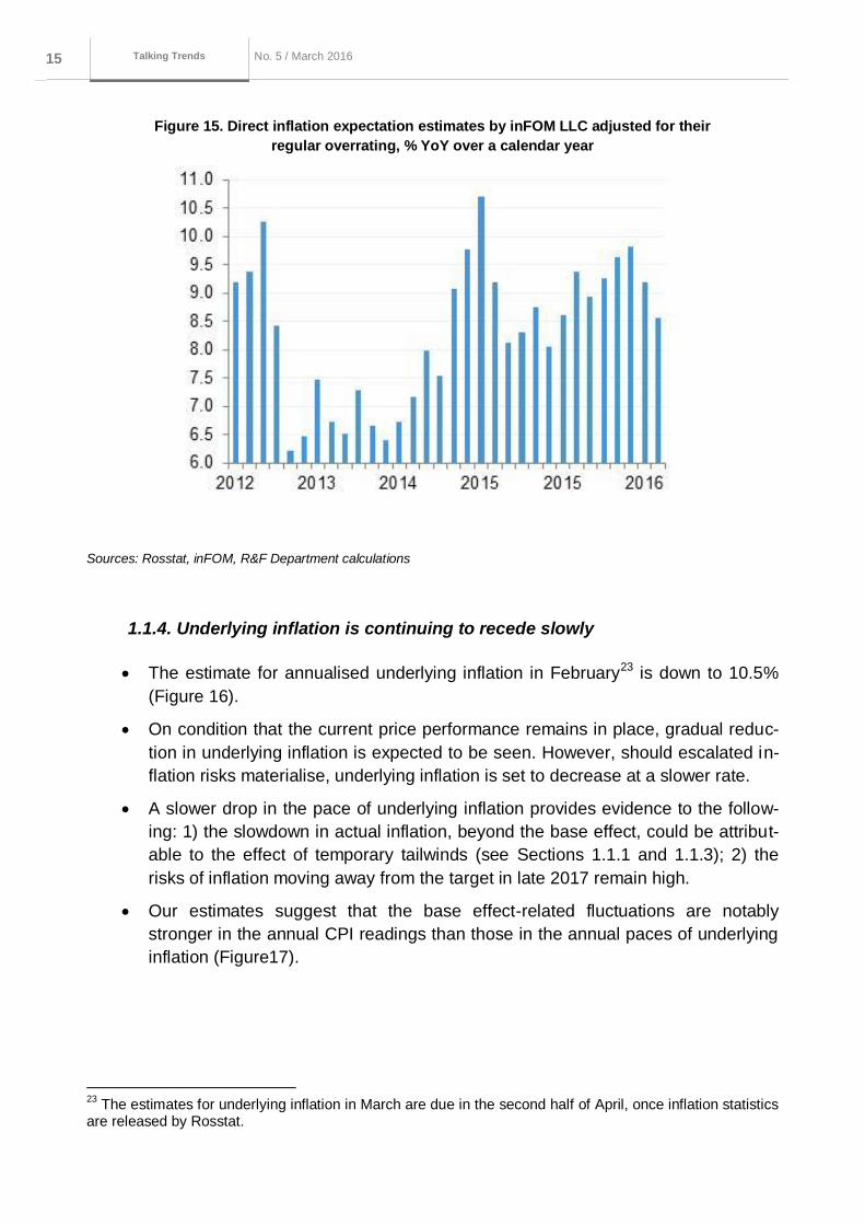
1.1.3. Inflation expectations in March: the drop has not been persistent
As seen from inFOM March survey, R&F Department-adjusted for systematic over-
statement, inflation expectations in March were down from 9.2% to 8.5% (Figure 15)22.
The pattern of inflation expectations is to a large degree determined by several
tailwinds that are most likely to be temporary. In this connection, it is premature to dis-
cuss a sustainable trend towards declining inflation expectations, with inflation risk re-
maining high.
22
For the calculation methodology please refer to the previous Bulletin issue (see Bulletin 'Talking Trends' No. 3. January 2016, Section 1.3.2 ‘Inflation expectations continue growing in January’).
Серия до кла до в о б э ко но мичеСких
иССледо ва ниях 15 No. 5 / March 2016
Macroeconomics and markets No. 1 / October
2015
Talking Trends
Figure 15. Direct inflation expectation estimates by inFOM LLC adjusted for their
regular overrating, % YoY over a calendar year
Sources: Rosstat, inFOM, R&F Department calculations
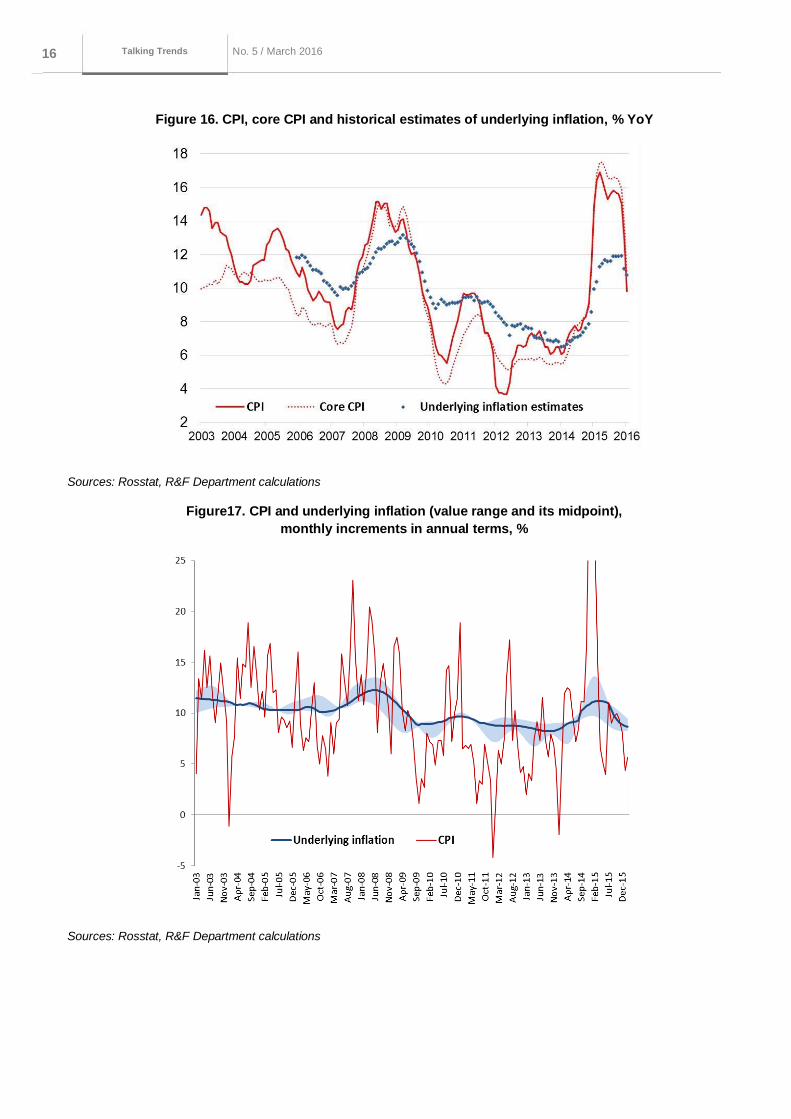
1.1.4. Underlying inflation is continuing to recede slowly
The estimate for annualised underlying inflation in February23 is down to 10.5%
(Figure 16).
On condition that the current price performance remains in place, gradual reduc-
tion in underlying inflation is expected to be seen. However, should escalated in-
flation risks materialise, underlying inflation is set to decrease at a slower rate.
A slower drop in the pace of underlying inflation provides evidence to the follow-
ing: 1) the slowdown in actual inflation, beyond the base effect, could be attribut-
able to the effect of temporary tailwinds (see Sections 1.1.1 and 1.1.3); 2) the
risks of inflation moving away from the target in late 2017 remain high.
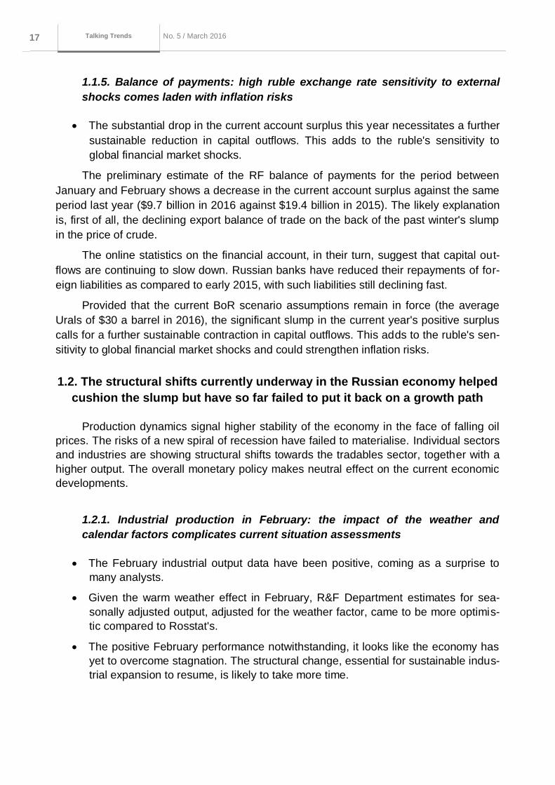
Our estimates suggest that the base effect-related fluctuations are notably
stronger in the annual CPI readings than those in the annual paces of underlying
inflation (Figure17).
23
The estimates for underlying inflation in March are due in the second half of April, once inflation statistics are released by Rosstat.
Серия до кла до в о б э ко но мичеСких
иССледо ва ниях 16 No. 5 / March 2016
Macroeconomics and markets No. 1 / October
2015
Talking Trends
Figure 16. CPI, core CPI and historical estimates of underlying inflation, % YoY
Sources: Rosstat, R&F Department calculations
Figure17. CPI and underlying inflation (value range and its midpoint),
monthly increments in annual terms, %
Sources: Rosstat, R&F Department calculations
Серия до кла до в о б э ко но мичеСких
иССледо ва ниях 17 No. 5 / March 2016
Macroeconomics and markets No. 1 / October
2015
Talking Trends
1.1.5. Balance of payments: high ruble exchange rate sensitivity to external
shocks comes laden with inflation risks
The substantial drop in the current account surplus this year necessitates a further
sustainable reduction in capital outflows. This adds to the ruble's sensitivity to
global financial market shocks.
The preliminary estimate of the RF balance of payments for the period between
January and February shows a decrease in the current account surplus against the same
period last year ($9.7 billion in 2016 against $19.4 billion in 2015). The likely explanation
is, first of all, the declining export balance of trade on the back of the past winter's slump
in the price of crude.
The online statistics on the financial account, in their turn, suggest that capital out-
flows are continuing to slow down. Russian banks have reduced their repayments of for-
eign liabilities as compared to early 2015, with such liabilities still declining fast.
Provided that the current BoR scenario assumptions remain in force (the average
Urals of $30 a barrel in 2016), the significant slump in the current year's positive surplus
calls for a further sustainable contraction in capital outflows. This adds to the ruble's sen-
sitivity to global financial market shocks and could strengthen inflation risks.
1.2. The structural shifts currently underway in the Russian economy helped
cushion the slump but have so far failed to put it back on a growth path
Production dynamics signal higher stability of the economy in the face of falling oil
prices. The risks of a new spiral of recession have failed to materialise. Individual sectors
and industries are showing structural shifts towards the tradables sector, together with a
higher output. The overall monetary policy makes neutral effect on the current economic
developments.
1.2.1. Industrial production in February: the impact of the weather and
calendar factors complicates current situation assessments
The February industrial output data have been positive, coming as a surprise to
many analysts.
Given the warm weather effect in February, R&F Department estimates for sea-
sonally adjusted output, adjusted for the weather factor, came to be more optimis-
tic compared to Rosstat's.
The positive February performance notwithstanding, it looks like the economy has
yet to overcome stagnation. The structural change, essential for sustainable indus-
trial expansion to resume, is likely to take more time.
Серия до кла до в о б э ко но мичеСких
иССледо ва ниях 18 No. 5 / March 2016
Macroeconomics and markets No. 1 / October
2015
Talking Trends
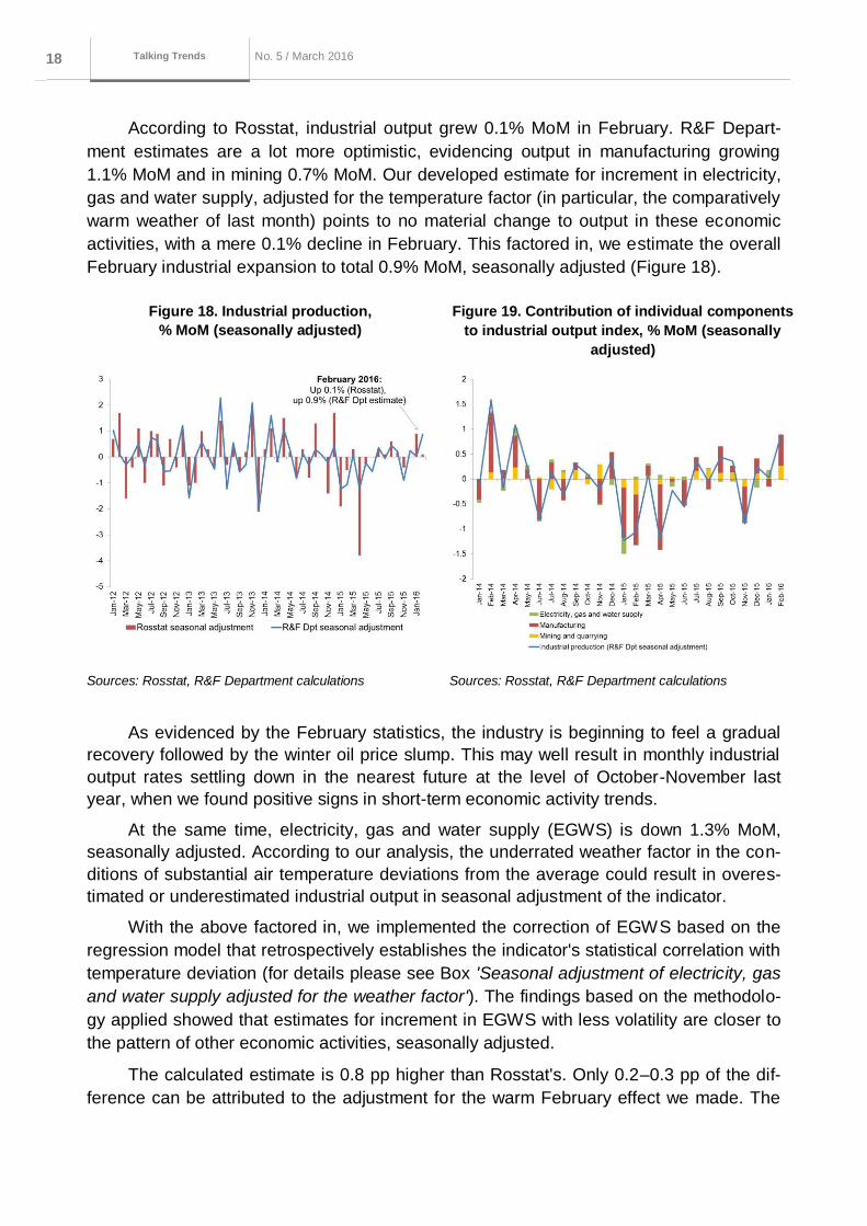
According to Rosstat, industrial output grew 0.1% MoM in February. R&F Depart-
ment estimates are a lot more optimistic, evidencing output in manufacturing growing
1.1% MoM and in mining 0.7% MoM. Our developed estimate for increment in electricity,
gas and water supply, adjusted for the temperature factor (in particular, the comparatively
warm weather of last month) points to no material change to output in these economic
activities, with a mere 0.1% decline in February. This factored in, we estimate the overall
February industrial expansion to total 0.9% MoM, seasonally adjusted (Figure 18).
Figure 18. Industrial production,
% MoM (seasonally adjusted)
Figure 19. Contribution of individual components
to industrial output index, % MoM (seasonally
adjusted)
Sources: Rosstat, R&F Department calculations Sources: Rosstat, R&F Department calculations
As evidenced by the February statistics, the industry is beginning to feel a gradual
recovery followed by the winter oil price slump. This may well result in monthly industrial
output rates settling down in the nearest future at the level of October-November last
year, when we found positive signs in short-term economic activity trends.
At the same time, electricity, gas and water supply (EGWS) is down 1.3% MoM,
seasonally adjusted. According to our analysis, the underrated weather factor in the con-
ditions of substantial air temperature deviations from the average could result in overes-
timated or underestimated industrial output in seasonal adjustment of the indicator.
With the above factored in, we implemented the correction of EGWS based on the
regression model that retrospectively establishes the indicator's statistical correlation with
temperature deviation (for details please see Box 'Seasonal adjustment of electricity, gas
and water supply adjusted for the weather factor'). The findings based on the methodolo-
gy applied showed that estimates for increment in EGWS with less volatility are closer to
the pattern of other economic activities, seasonally adjusted.
The calculated estimate is 0.8 pp higher than Rosstat's. Only 0.2–0.3 pp of the dif-
ference can be attributed to the adjustment for the warm February effect we made. The
Серия до кла до в о б э ко но мичеСких
иССледо ва ниях 19 No. 5 / March 2016
Macroeconomics and markets No. 1 / October
2015
Talking Trends
remainder of 0.5-0.6 pp must be the difference in other seasonal adjustment criteria.
Practice shows that, with short-term indicators being unstable, the resulting seasonal ad-
justment may well be sensitive enough not only to the seasonal adjustment methodology
(e.g.,TRAMO/SEATS, X12-ARIMA) but to the historical selection applied, the procedures
for automatic model selection and quality assurance of seasonal adjustment outcomes, to
the calendar effect removal approach, identification of outliers, etc.
While we are on the February, the leap year's positive effect should be noted in the
context of industrial production and overall economic developments. With the number of
work days in February this year unchanged as last year, the extra calendar day was sup-
posed to make a positive effect on the economy. This should manifest itself through the
consumption of products and services.
Regardless of the overall optimistic findings, we continue to treat the recently avail-
able statistics with caution, as long as the high volatility in monthly data remains, and in
view of the substantial difference in seasonally adjusted growth increment estimates from
Rosstat's.
Seasonal adjustment of electricity,
gas and water supply adjusted for the weather factor
The expansion in the EGWS is due to the weather conditions, while control of this factor is es-
sential as seasonally adjusted estimates for industrial output are made.
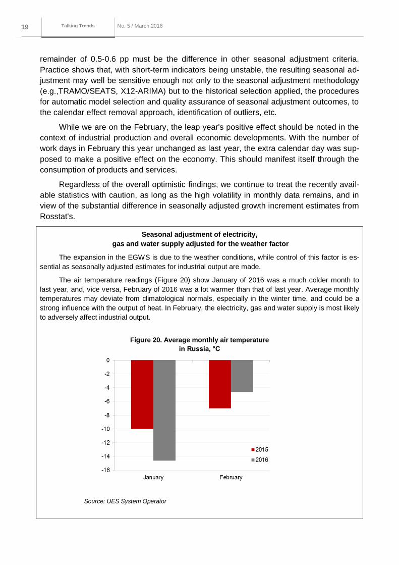
The air temperature readings (Figure 20) show January of 2016 was a much colder month to
last year, and, vice versa, February of 2016 was a lot warmer than that of last year. Average monthly
temperatures may deviate from climatological normals, especially in the winter time, and could be a
strong influence with the output of heat. In February, the electricity, gas and water supply is most likely
to adversely affect industrial output.
Figure 20. Average monthly air temperature
in Russia, °C
Source: UES System Operator
Серия до кла до в о б э ко но мичеСких
иССледо ва ниях 20 No. 5 / March 2016
Macroeconomics and markets No. 1 / October
2015
Talking Trends
We carried out direct comparison of the deviated seasonally adjusted EGW production to the
average output rates in mining and manufacturing, on the one hand, and the excess of climatic normal
across Russia, on the other. We were especially focused on the instances where seasonally adjusted
deviations in EGWS were substantial and in excess of 1 pp, most probably as a result of the underval-
ued weather factor from the standpoint of seasonal adjustment.
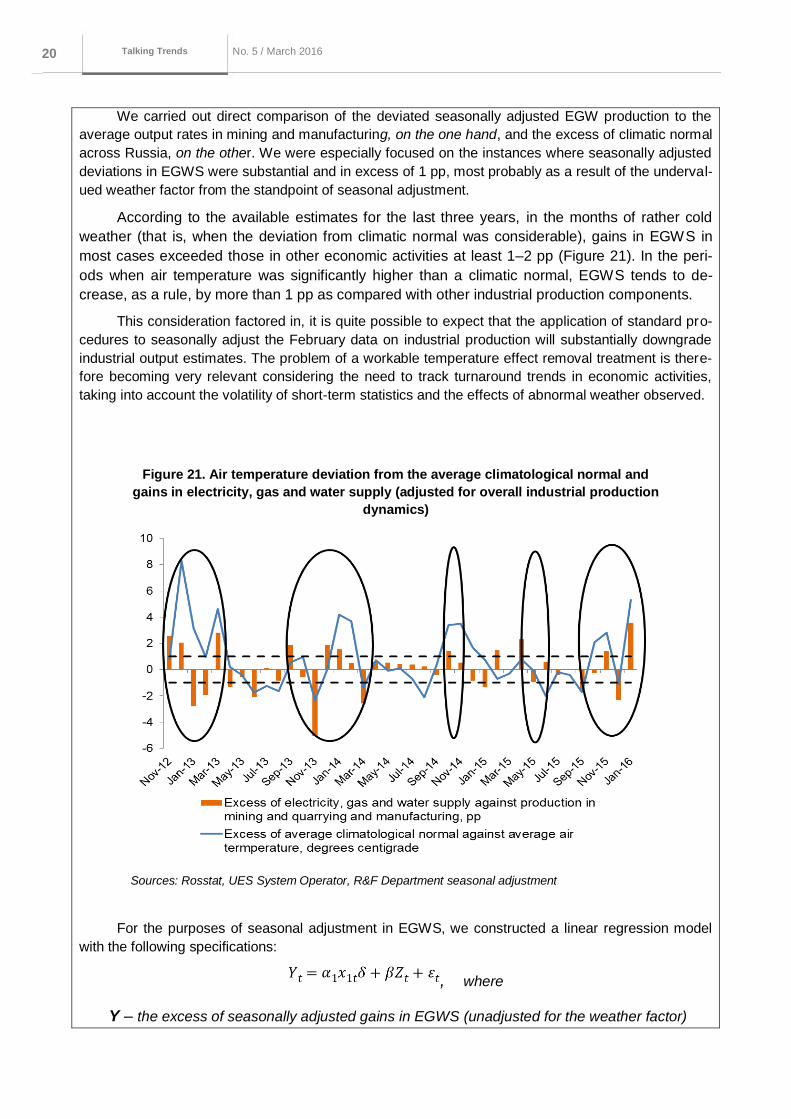
According to the available estimates for the last three years, in the months of rather cold
weather (that is, when the deviation from climatic normal was considerable), gains in EGWS in
most cases exceeded those in other economic activities at least 1–2 pp (Figure 21). In the peri-
ods when air temperature was significantly higher than a climatic normal, EGWS tends to de-
crease, as a rule, by more than 1 pp as compared with other industrial production components.
This consideration factored in, it is quite possible to expect that the application of standard pro-
cedures to seasonally adjust the February data on industrial production will substantially downgrade
industrial output estimates. The problem of a workable temperature effect removal treatment is there-
fore becoming very relevant considering the need to track turnaround trends in economic activities,
taking into account the volatility of short-term statistics and the effects of abnormal weather observed.
Figure 21. Air temperature deviation from the average climatological normal and
gains in electricity, gas and water supply (adjusted for overall industrial production
dynamics)
Sources: Rosstat, UES System Operator, R&F Department seasonal adjustment
For the purposes of seasonal adjustment in EGWS, we constructed a linear regression model
with the following specifications:
, where
Y – the excess of seasonally adjusted gains in EGWS (unadjusted for the weather factor)
Серия до кла до в о б э ко но мичеСких
иССледо ва ниях 21 No. 5 / March 2016
Macroeconomics and markets No. 1 / October
2015
Talking Trends
against production gains in other economic activities (mining and manufacturing);
– the excess over the average climatological normal air temperature (centigrade, according to
UES Central Dispatch Office (CDO));
– other explanatory factors matrix;
dummy-variable, equal to one for the winter season (November through March
inclusive), and zero in the rest of the months;
,β – unknown estimated parameter vectors;
– random error.
The above-mentioned regression model enabled us to extend this conclusion to all previous
time periods, so we can test the hypothesis that there is a statistically significant interrelation between
air temperature deviations and electricity, gas and water supply pattern.
The dummy variable included into the model enabled us to separate conditionally winter
months when power generation is allegedly more sensitive to weather anomalies (these comprised
November, December, January, February and March), as distinct from the rest of the months, and to
estimate the regression equation, taking into account, inter alia, these observations only.
Equation parametrisation through the usual of the least-squares method yielded the estimate of
the key coefficient ,which was statistically significant with a 95-percent level of trust. This
elasticity also has the 'correct' sign, that is, the warmer (colder) the winter period is against the clima-
tologic normal, the more upgrade / downgrade in production (electricity, gas and water) is shown by
the traditional seasonal adjustment without correction for temperature. Plus, if model parametrisation
is conducted for the other warmer months, the corresponding estimate, to support our original hypoth-
esis, is substantially lower - , and yet it happens to be negative and statistically significant.
Taking into account the resulting estimates the corrected seasonally adjusted assessment of
EGWS increment ( )) was thereafter calculated without correction for the weather factor
and the air temperature deviation ( ) according to formulas:
- for the period between November and March inclusive;
- for the period between April and October inclusive;
Seasonally adjusted increments were therefore corrected for the amount of their 'temperature-
determined' fluctuations versus output in other economic activities.
The important conclusion following from the analysis we carried out is that seasonal adjustment
in EGWS with recognition of the weather factor not only eliminates alleged excessive and low informa-
tive volatility from the row dynamics. The dynamics in the modified row become much closer to output
fluctuations in manufacturing, which is, in terms of gross value added (GVA), is the most powerful
component in industrial production (Figure 22), that is, it becomes more correlated with the general
state of affairs in manufacturing. Over the last year and a half, it is most clearly seen in the winter pe-
Серия до кла до в о б э ко но мичеСких
иССледо ва ниях 22 No. 5 / March 2016
Macroeconomics and markets No. 1 / October
2015
Talking Trends
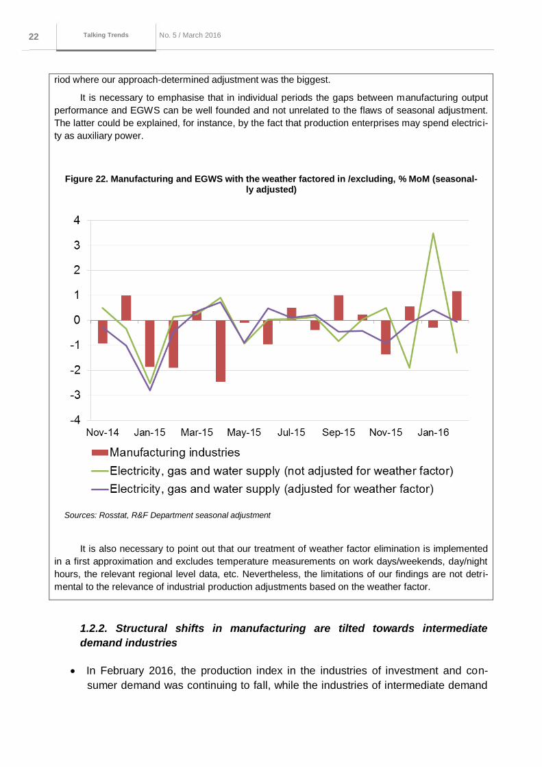
riod where our approach-determined adjustment was the biggest.
It is necessary to emphasise that in individual periods the gaps between manufacturing output
performance and EGWS can be well founded and not unrelated to the flaws of seasonal adjustment.
The latter could be explained, for instance, by the fact that production enterprises may spend electrici-
ty as auxiliary power.
Figure 22. Manufacturing and EGWS with the weather factored in /excluding, % MoM (seasonal-ly adjusted)
Sources: Rosstat, R&F Department seasonal adjustment
It is also necessary to point out that our treatment of weather factor elimination is implemented
in a first approximation and excludes temperature measurements on work days/weekends, day/night
hours, the relevant regional level data, etc. Nevertheless, the limitations of our findings are not detri-
mental to the relevance of industrial production adjustments based on the weather factor.
1.2.2. Structural shifts in manufacturing are tilted towards intermediate
demand industries
In February 2016, the production index in the industries of investment and con-
sumer demand was continuing to fall, while the industries of intermediate demand
Серия до кла до в о б э ко но мичеСких
иССледо ва ниях 23 No. 5 / March 2016
Macroeconomics and markets No. 1 / October
2015
Talking Trends
saw a strengthening in the trend towards growth, reflecting the current structural
shifts.
As compared to the 2008-2009 recession, the current changes to the output
structure are less intensive but are advancing progressively, being primarily of a
structural, not cyclical, nature.
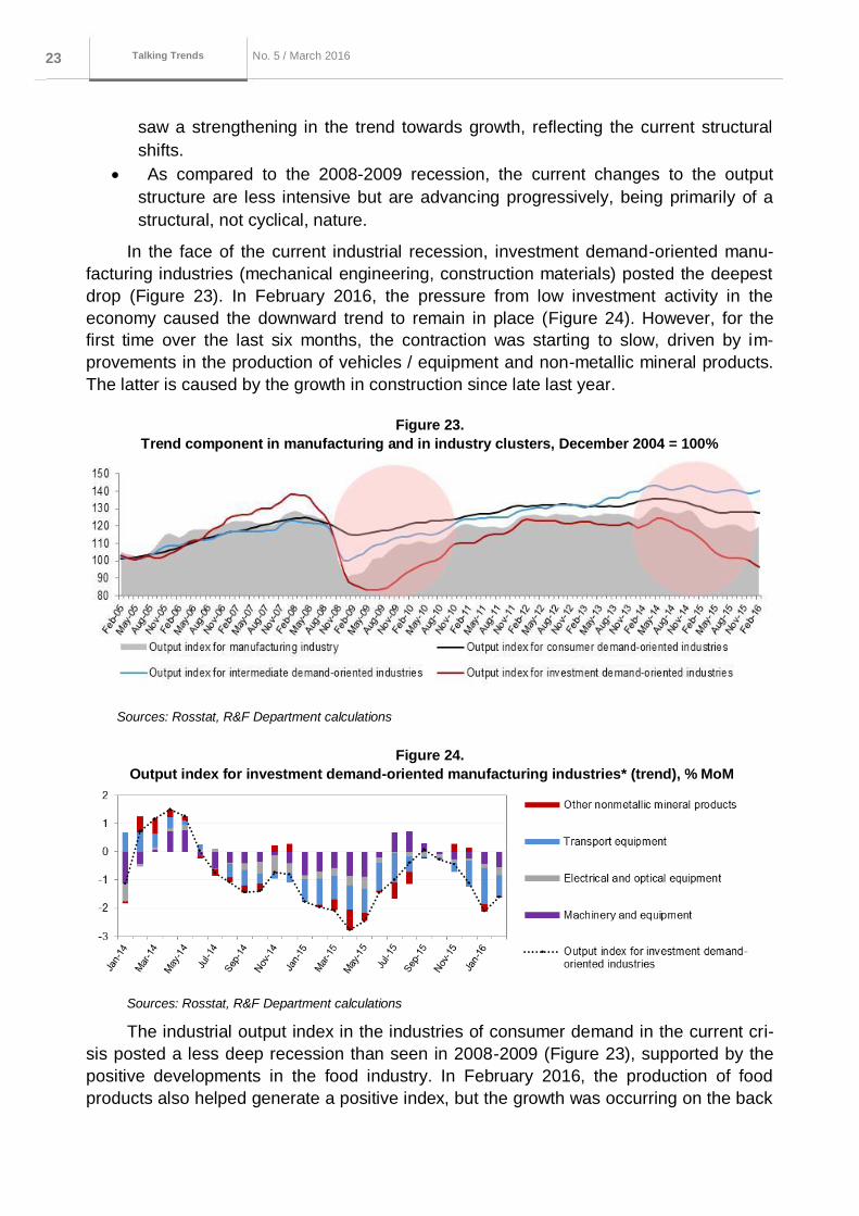
In the face of the current industrial recession, investment demand-oriented manu-
facturing industries (mechanical engineering, construction materials) posted the deepest
drop (Figure 23). In February 2016, the pressure from low investment activity in the
economy caused the downward trend to remain in place (Figure 24). However, for the
first time over the last six months, the contraction was starting to slow, driven by im-
provements in the production of vehicles / equipment and non-metallic mineral products.
The latter is caused by the growth in construction since late last year.
Figure 23.
Trend component in manufacturing and in industry clusters, December 2004 = 100%
Sources: Rosstat, R&F Department calculations
Figure 24.
Output index for investment demand-oriented manufacturing industries* (trend), % MoM
Sources: Rosstat, R&F Department calculations
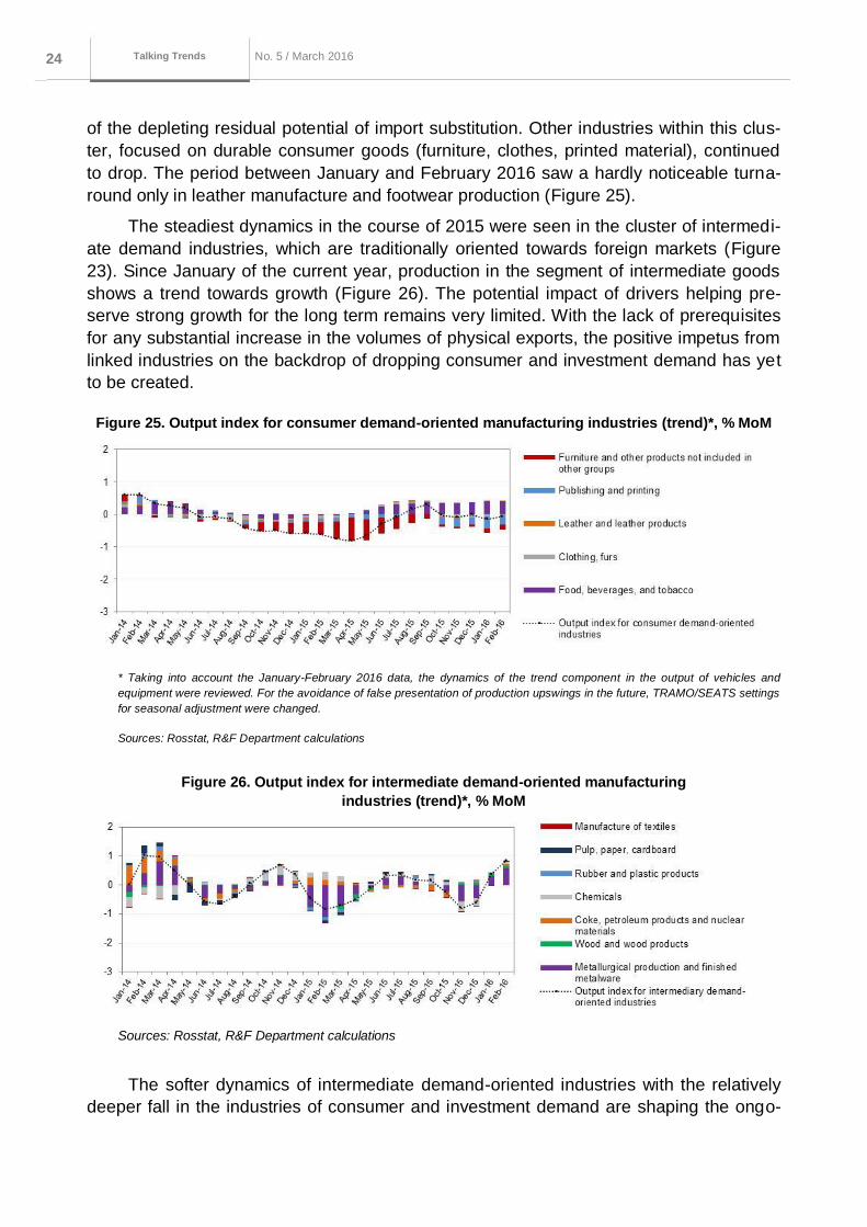
The industrial output index in the industries of consumer demand in the current cri-
sis posted a less deep recession than seen in 2008-2009 (Figure 23), supported by the
positive developments in the food industry. In February 2016, the production of food
products also helped generate a positive index, but the growth was occurring on the back
Серия до кла до в о б э ко но мичеСких
иССледо ва ниях 24 No. 5 / March 2016
Macroeconomics and markets No. 1 / October
2015
Talking Trends
of the depleting residual potential of import substitution. Other industries within this clus-
ter, focused on durable consumer goods (furniture, clothes, printed material), continued
to drop. The period between January and February 2016 saw a hardly noticeable turna-
round only in leather manufacture and footwear production (Figure 25).
The steadiest dynamics in the course of 2015 were seen in the cluster of intermedi-
ate demand industries, which are traditionally oriented towards foreign markets (Figure
23). Since January of the current year, production in the segment of intermediate goods
shows a trend towards growth (Figure 26). The potential impact of drivers helping pre-
serve strong growth for the long term remains very limited. With the lack of prerequisites
for any substantial increase in the volumes of physical exports, the positive impetus from
linked industries on the backdrop of dropping consumer and investment demand has yet
to be created.
Figure 25. Output index for consumer demand-oriented manufacturing industries (trend)*, % MoM
* Taking into account the January-February 2016 data, the dynamics of the trend component in the output of vehicles and
equipment were reviewed. For the avoidance of false presentation of production upswings in the future, TRAMO/SEATS settings
for seasonal adjustment were changed.
Sources: Rosstat, R&F Department calculations
Figure 26. Output index for intermediate demand-oriented manufacturing
industries (trend)*, % MoM
Sources: Rosstat, R&F Department calculations
The softer dynamics of intermediate demand-oriented industries with the relatively
deeper fall in the industries of consumer and investment demand are shaping the ongo-
Серия до кла до в о б э ко но мичеСких
иССледо ва ниях 25 No. 5 / March 2016
Macroeconomics and markets No. 1 / October
2015
Talking Trends
ing structural shifts in manufacturing. This direction of structural shifts is understood to be
quite natural for the economy focused on export of raw materials and low added value
products.
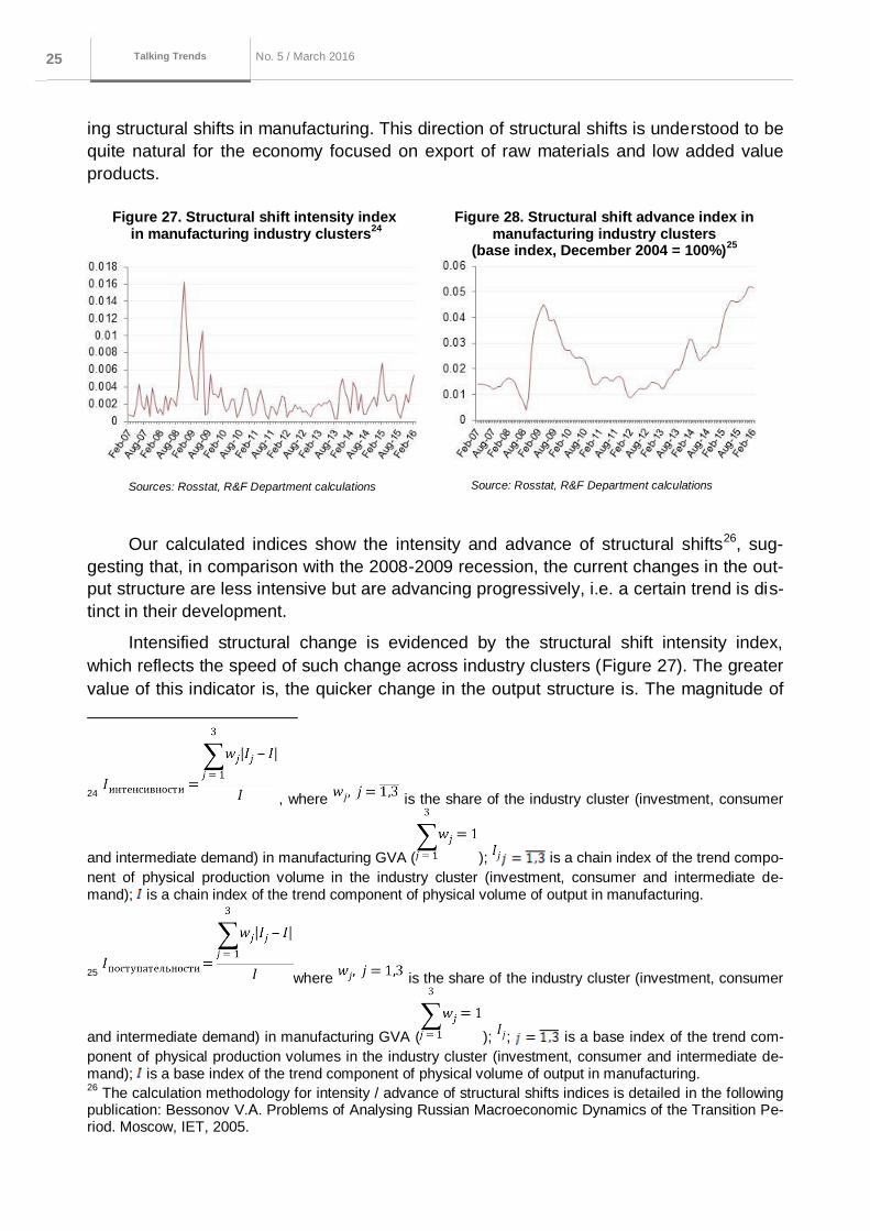
Figure 27. Structural shift intensity index in manufacturing industry clusters
24
Figure 28. Structural shift advance index in manufacturing industry clusters
(base index, December 2004 = 100%)25
Sources: Rosstat, R&F Department calculations
Source: Rosstat, R&F Department calculations
Our calculated indices show the intensity and advance of structural shifts26, sug-
gesting that, in comparison with the 2008-2009 recession, the current changes in the out-
put structure are less intensive but are advancing progressively, i.e. a certain trend is dis-
tinct in their development.
Intensified structural change is evidenced by the structural shift intensity index,
which reflects the speed of such change across industry clusters (Figure 27). The greater
value of this indicator is, the quicker change in the output structure is. The magnitude of
24 , where is the share of the industry cluster (investment, consumer
and intermediate demand) in manufacturing GVA ( ); is a chain index of the trend compo-
nent of physical production volume in the industry cluster (investment, consumer and intermediate de-mand); is a chain index of the trend component of physical volume of output in manufacturing.
25 where is the share of the industry cluster (investment, consumer
and intermediate demand) in manufacturing GVA ( ); ; is a base index of the trend com-
ponent of physical production volumes in the industry cluster (investment, consumer and intermediate de-mand); is a base index of the trend component of physical volume of output in manufacturing. 26
The calculation methodology for intensity / advance of structural shifts indices is detailed in the following publication: Bessonov V.А. Problems of Analysing Russian Macroeconomic Dynamics of the Transition Pe-riod. Moscow, IET, 2005.
Серия до кла до в о б э ко но мичеСких
иССледо ва ниях 26 No. 5 / March 2016
Macroeconomics and markets No. 1 / October
2015
Talking Trends
index variation came up against 2014, albeit to a less extent compared to the 2008-2009
crisis. This suggests a slower materialisation of structural change in the current economic
slump. Less intensive though these shifts may be, they are not the outcome of sporadic
output fluctuations and are advancing progressively. This is supported by the advance of
structural shifts indicator, with an upward trend since 2013. In 2008-2009, the structural
shift advance index underwent strong yet short-term fluctuations of irregular nature, driv-
en by the cyclical, rather than structural, nature of the change at the time (Figure 28).
The intensity and advance of structural shift indices are inconclusive as to how qual-
itative the nature of change is in manufacturing and if this change comes with a growing
share of high value added products. As mentioned above, since early 2014 we have been
seeing that the drop in the production of consumer and investment demand products, that
is, higher value added products, has been outpacing that in intermediate demand prod-
ucts. And this indirectly points to worsened quality of the industrial output in manufactur-
ing.
1.2.3. The rising output in key industries in February should not be
overinterpreted
Although the output in the key industries in February did grow, it would be prema-
ture to envisage the start of recovery growth.
The regional key industry index shows better economic performance on last year
in almost all federal districts, in many ways thanks to the leap year effect and the
low base of February of the past year.
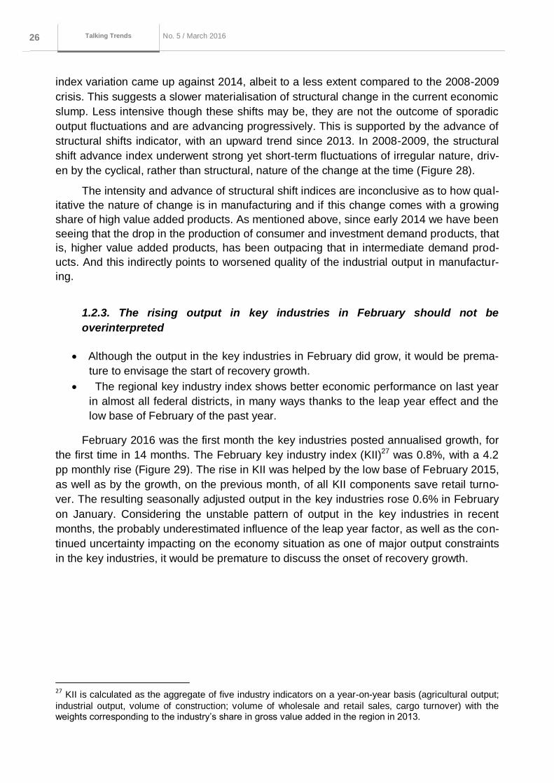
February 2016 was the first month the key industries posted annualised growth, for
the first time in 14 months. The February key industry index (KII)27 was 0.8%, with a 4.2
pp monthly rise (Figure 29). The rise in KII was helped by the low base of February 2015,
as well as by the growth, on the previous month, of all KII components save retail turno-
ver. The resulting seasonally adjusted output in the key industries rose 0.6% in February
on January. Considering the unstable pattern of output in the key industries in recent
months, the probably underestimated influence of the leap year factor, as well as the con-
tinued uncertainty impacting on the economy situation as one of major output constraints
in the key industries, it would be premature to discuss the onset of recovery growth.
27
KII is calculated as the aggregate of five industry indicators on a year-on-year basis (agricultural output;
industrial output, volume of construction; volume of wholesale and retail sales, cargo turnover) with the weights corresponding to the industry’s share in gross value added in the region in 2013.
Серия до кла до в о б э ко но мичеСких
иССледо ва ниях 27 No. 5 / March 2016
Macroeconomics and markets No. 1 / October
2015
Talking Trends
Figure 29. Industrial components’ contribution to KII behaviour in Russia in 2014-2016, % YoY
Sources: Rosstat, R&F Department calculations
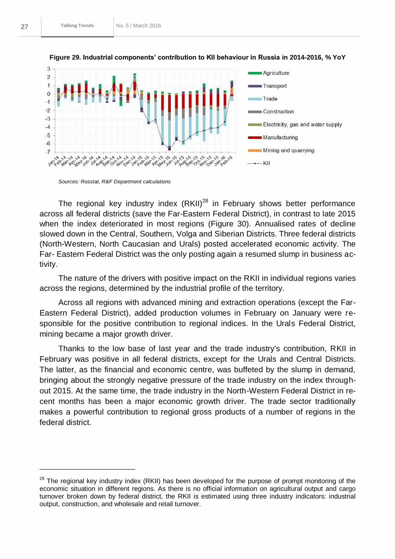
The regional key industry index (RKII)28 in February shows better performance
across all federal districts (save the Far-Eastern Federal District), in contrast to late 2015
when the index deteriorated in most regions (Figure 30). Annualised rates of decline
slowed down in the Central, Southern, Volga and Siberian Districts. Three federal districts
(North-Western, North Caucasian and Urals) posted accelerated economic activity. The
Far- Eastern Federal District was the only posting again a resumed slump in business ac-
tivity.
The nature of the drivers with positive impact on the RKII in individual regions varies
across the regions, determined by the industrial profile of the territory.
Across all regions with advanced mining and extraction operations (except the Far-
Eastern Federal District), added production volumes in February on January were re-
sponsible for the positive contribution to regional indices. In the Urals Federal District,
mining became a major growth driver.
Thanks to the low base of last year and the trade industry's contribution, RKII in
February was positive in all federal districts, except for the Urals and Central Districts.
The latter, as the financial and economic centre, was buffeted by the slump in demand,
bringing about the strongly negative pressure of the trade industry on the index through-
out 2015. At the same time, the trade industry in the North-Western Federal District in re-
cent months has been a major economic growth driver. The trade sector traditionally
makes a powerful contribution to regional gross products of a number of regions in the
federal district.
28
The regional key industry index (RKII) has been developed for the purpose of prompt monitoring of the economic situation in different regions. As there is no official information on agricultural output and cargo turnover broken down by federal district, the RKII is estimated using three industry indicators: industrial output, construction, and wholesale and retail turnover.
Серия до кла до в о б э ко но мичеСких
иССледо ва ниях 28 No. 5 / March 2016
Macroeconomics and markets No. 1 / October
2015
Talking Trends
Figure 30. Industrial components’ contribution to RKII growth in 2015-2016, % YoY
Sources: Rosstat, R&F Department calculations
February's output in manufacturing grew against January only in the North Cauca-
sian and Urals Federal Districts. In the latter, increased production volumes are accom-
panied with the advancement of processing sectors which are linked to the oil industry:
coke, petroleum products, and chemicals. In North Caucasus, the positive growth rates in
manufacturing are driven by the launch of the new gas-processing plant in the Stavropol
Territory, as well as by expanding production of vehicles and equipment in the Republic
of Daghestan (possibly, in the context of the defense order).
Central Federal District North-Western Federal District Southern Federal District
North Caucasian Federal District Volga Federal District Urals Federal District
Siberian Federal District Far-Eastern Federal District
Серия до кла до в о б э ко но мичеСких
иССледо ва ниях 29 No. 5 / March 2016
Macroeconomics and markets No. 1 / October
2015
Talking Trends
1.2.4. March PMI survey, production: growth is on hold
The notable decrease in employment, output and new orders indices (PMI) leads
to conclude that the industrial dynamics of early Q2 macroeconomic indicators
might come in weak.
PMI in manufacturing industries in Russia in March was substantially worse than
expectations. The stabilisation of the index close to the border zone (50 points), observed
for the last few months, was followed by the drop to a minimum seen since July 2015 to
48.3 points. Strong deterioration was seen in the employment component decreasing to
45.6 points, a minimum since January 2015 and can be indicative of intensified lay-off
processes.
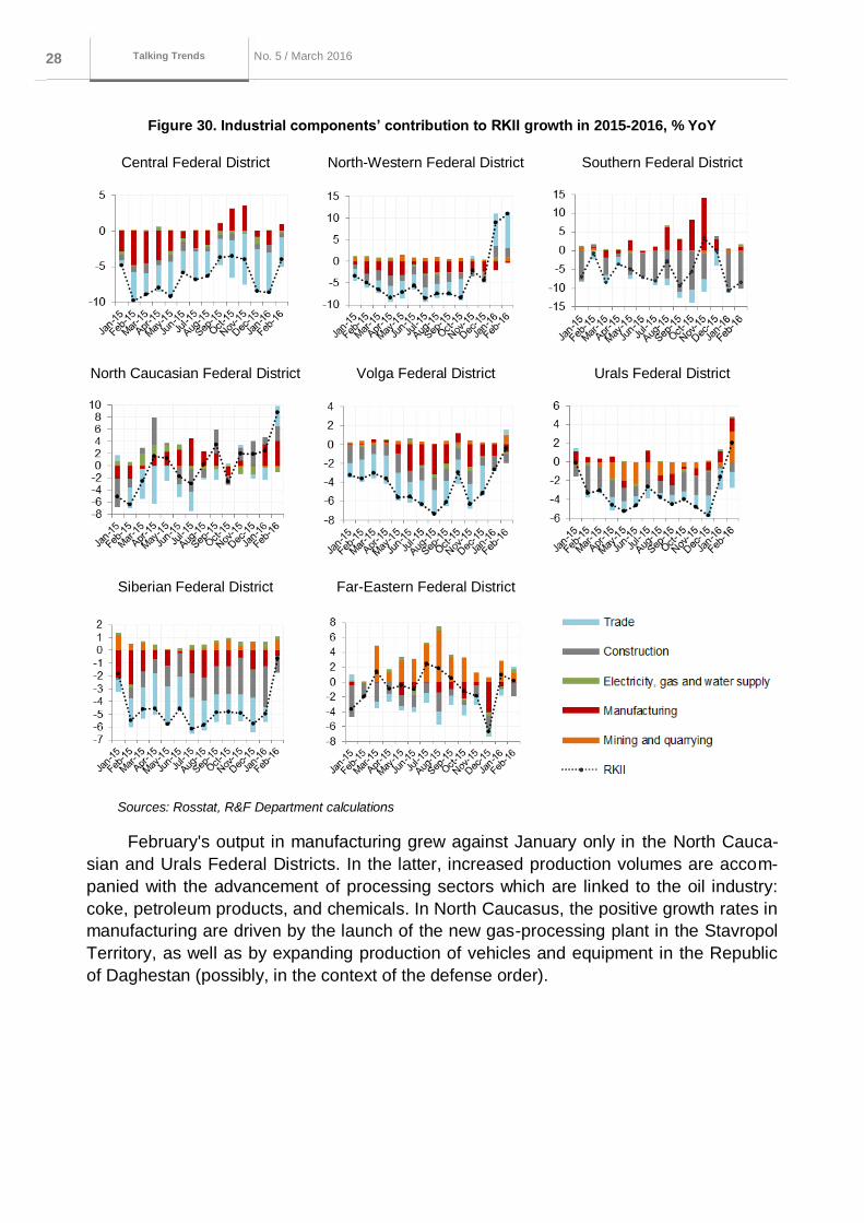
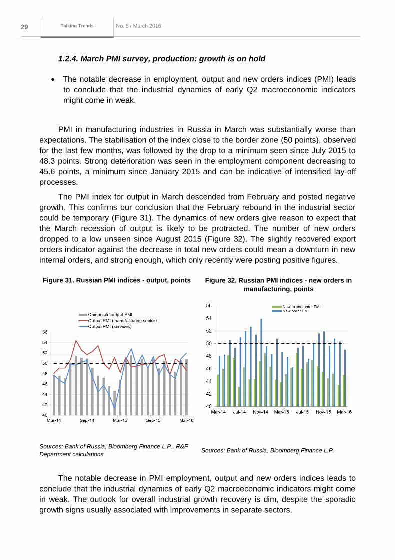
The PMI index for output in March descended from February and posted negative
growth. This confirms our conclusion that the February rebound in the industrial sector
could be temporary (Figure 31). The dynamics of new orders give reason to expect that
the March recession of output is likely to be protracted. The number of new orders
dropped to a low unseen since August 2015 (Figure 32). The slightly recovered export
orders indicator against the decrease in total new orders could mean a downturn in new
internal orders, and strong enough, which only recently were posting positive figures.
Figure 31. Russian PMI indices - output, points Figure 32. Russian PMI indices - new orders in
manufacturing, points
Sources: Bank of Russia, Bloomberg Finance L.P., R&F
Department calculations Sources: Bank of Russia, Bloomberg Finance L.P.
The notable decrease in PMI employment, output and new orders indices leads to
conclude that the industrial dynamics of early Q2 macroeconomic indicators might come
in weak. The outlook for overall industrial growth recovery is dim, despite the sporadic
growth signs usually associated with improvements in separate sectors.
Серия до кла до в о б э ко но мичеСких
иССледо ва ниях 30 No. 5 / March 2016
Macroeconomics and markets No. 1 / October
2015
Talking Trends
Importantly, the February and March PMI indices may to a degree misrepresent the
real picture. Seasonally adjusted PMI indicators may underrate the leap-year effect. This
may well result in the February PMI readings to be overestimated, and March – underes-
timated. In this context, the April data can provide more insight into the current state of
indicators.
1.2.5. Unemployment remains stable
In the face of stable unemployment indicators, labour resources are slowly over-
flowing from the non-tradables sector (construction, finance) to tradables (produc-
tion, chemistry, etc.).
Low labour mobility, coupled with Russian demographic specifics, and growing
informal employment may well slow down the economic transition to a new bal-
ance and prolong the stagnation period.
According to Rosstat, February's unemployment remained level with January at
5.84% (Figure 33). Unemployment (unadjusted for the seasonal factor) decreased from
5.6% in January to 5.5% in February. For the fourth month in a row (since November
2015), the number of unemployed remains on the order of 4.4 million people, which is 0.4
million higher than the minimum value seen in June 2015. Since the beginning of 2016,
the intensive lay-off processes have been slowing down.
In addition to Rosstat-calculated unemployment rate, we calculated broader U5 and
U629 unemployment rates (Figure 34). At the end of 2015, U5 was growing. It occurred on
the back of withdrawal of part of the population from estimated workforce30. Amid eco-
nomic uncertainty and economic downturn, businesses were forced to reduce manpower
resources, showing, at the end of 2015, weaker demand for labour.
U6 is also growing, albeit slower than U5. Businesses are still attempting to escape
large-scale staff reductions as they switch, if necessary, to the partial employment mode
(less than 30 hours) for some of their staff. This argument is further supported by Rosstat
data showing the growth of working population looking for a side job.
29
This classification is applied for calculation of various Bureau of Labor Statistics of indicators (US Bureau of Labor Statistics). Their calculation is based on quarterly statistical data. The U5 indicator, beyond the registered number of unemployed, includes economically inactive population, that is, people who are not looking for a job or who lost hope to find it but are still willing to work. The U6 indicator includes U5 and those occupied part-time (less than 30 hours a week). 30
Some part of the population stops looking for a job and is technically excluded from workforce.

Серия до кла до в о б э ко но мичеСких
иССледо ва ниях 31 No. 5 / March 2016
Macroeconomics and markets No. 1 / October
2015
Talking Trends
Figure 33. Unemployment rate*, % Figure 34. Unemployment rate,
including part-time employment
and willingness to work, %
Sources: Rosstat, R&F Department calculations Sources: Rosstat, R&F Department calculations
In January 2016, the total number of occupied jobs fell 3% YoY. The number of jobs
for the period under review is continuing to drop across all types of economic activity, with
very few exceptions. The deepest slump is posted by the financial sector and construc-
tion, 11% and 10% respectively. The trade industry, manufacturing, the public sector and
energy generation and distribution posted a slightly less than 4% drop. Positive dynamics
are posted by the hotel and restaurant business with their 3.0% YoY growth, as well as
by some manufacturing subsectors (petroleum products with its 3.2% growth, chemicals
– 0.3%) and the extraction of fossil fuels subsector – 1.5%.
Overall, these dynamics are indicative of the ongoing labour force overflow from the
non-tradables sector (construction, finance) to tradables (mining and field production,
chemicals etc.) expected to materialise in the context of the change in foreign trade and
in relative prices. Yet, the scale of this change is too minor as compared to the develop-
ments from the viewpoint of structural economic transformation. Low labour mobility,
coupled with Russian demographic specifics, and growing informal employment, may well
slow down the economic transition to a new balance.
1.2.6. Russian producers remain competitive over their Chinese counterparts
on the back of a stronger yuan
Growth of nominal salaries within the last two years slightly outpaces China's
GDP growth. And, the growth of salaries in Russia in the current crisis remain
high taking into account the current performance …
… which enables China to boost, since the middle of 2014, the competitiveness
of its industry in terms of unit labour costs against Russia …
Серия до кла до в о б э ко но мичеСких
иССледо ва ниях 32 No. 5 / March 2016
Macroeconomics and markets No. 1 / October
2015
Talking Trends
however, the lost competitiveness of the Russian industry against China in terms
of salary growth was completely set off by the recent strengthening of nominal
yuan versus the ruble.
We compared the Russian and Chinese industries competitiveness in terms of unit
labour costs (further – ULC, from the English term). According to the commonly accepted
method for calculation of this indicator for various countries, officially in use by the Organ-
isation for Economic Cooperation and Development (OECD) and Eurostat, it is defined as
the ratio of the nominal wages fund (that is, the product of an average nominal salary
times the total employees) to the real output.
Taking into account the commodity structure of Chinese exports, it would be rea-
sonable to carry out production competitiveness analysis to that of trading partners oper-
ating the corresponding indicators (the average nominal salary, the number of employed
and output) only in relation to the processing sector.
We concluded this benchmark analysis premised on the restrictions of the available
data, first of all on China, looking into ULC quarterly performance for 2008-2015.
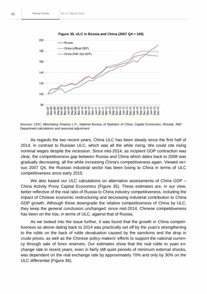
Figure 35 shows that the competitiveness of Russian products in terms of ULC was
growing versus China at the beginning of 2009 and in the middle of 2014 as the labour
market was adjusting to the crisis in the economy. However, these intervals were rather
an exception to the general rule. The trend towards rising salaries was clear in China until
recently, offsetting China's competitive advantages of cheap labour.
This comes as a result of a series of objective factors. First, this is gradual depletion
of the catching-up economic growth model, which has for long set GDP and, respectively,
salaries, to grow faster than in more developed economies. Secondly, it is explained by
tightened competition in the industrial areas in the face of China-pursued demographic
policies. The current situation shows that the long-term salary expansion trend seen until
recently is one of the key constraining factors for the Chinese economy.
Серия до кла до в о б э ко но мичеСких
иССледо ва ниях 33 No. 5 / March 2016
Macroeconomics and markets No. 1 / October
2015
Talking Trends
Figure 35. ULC in Russia and China (2007 Q4 = 100)
Sources: CEIC, Bloomberg Finance L.P., National Bureau of Statistics of China, Capital Economics, Rosstat, R&F
Department calculations and seasonal adjustment
As regards the two recent years, China ULC has been steady since the first half of
2014, in contrast to Russian ULC, which was all the while rising. We could cite rising
nominal wages despite the recession. Since mid-2014, as incipient GDP contraction was
clear, the competitiveness gap between Russia and China which dates back to 2008 was
gradually decreasing, all the while increasing China's competitiveness again. Viewed ver-
sus 2007 Q4, the Russian industrial sector has been losing to China in terms of ULC
competitiveness since early 2015.
We also based our ULC calculations on alternative assessments of China GDP –
China Activity Proxy Capital Economics (Figure 35). These estimates are, in our view,
better reflective of the real ratio of Russia to China industry competitiveness, including the
impact of Chinese economic restructuring and decreasing industrial contribution to China
GDP growth. Although these downgrade the relative competitiveness of China by ULC,
they keep the general conclusion unchanged: since mid-2014, Chinese competitiveness
has been on the rise, in terms of ULC, against that of Russia.
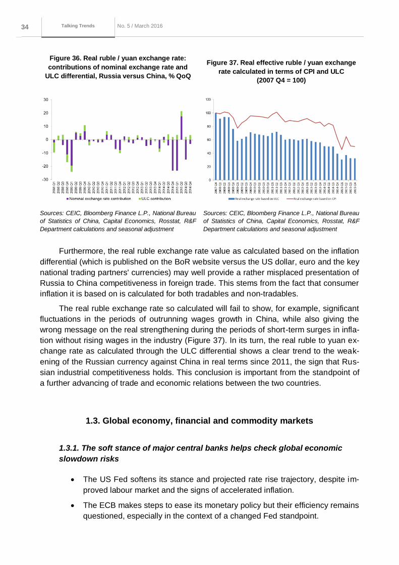
As we looked into the issue further, it was found that the growth in China competi-
tiveness as above dating back to 2014 was practically set off by the yuan's strengthening
to the ruble on the back of ruble devaluation caused by the sanctions and the drop in
crude prices, as well as the Chinese policy-makers' efforts to support the national curren-
cy through sale of forex reserves. Our estimates show that the real ruble to yuan ex-
change rate in recent years, even in fairly still quiet periods of minimum external shocks,
was dependent on the real exchange rate by approximately 70% and only by 30% on the
ULC differential (Figure 36).
Серия до кла до в о б э ко но мичеСких
иССледо ва ниях 34 No. 5 / March 2016
Macroeconomics and markets No. 1 / October
2015
Talking Trends
Figure 36. Real ruble / yuan exchange rate:
contributions of nominal exchange rate and
ULC differential, Russia versus China, % QoQ
Figure 37. Real effective ruble / yuan exchange
rate calculated in terms of CPI and ULC
(2007 Q4 = 100)
Sources: CEIC, Bloomberg Finance L.P., National Bureau
of Statistics of China, Capital Economics, Rosstat, R&F
Department calculations and seasonal adjustment
Sources: CEIC, Bloomberg Finance L.P., National Bureau
of Statistics of China, Capital Economics, Rosstat, R&F
Department calculations and seasonal adjustment
Furthermore, the real ruble exchange rate value as calculated based on the inflation
differential (which is published on the BoR website versus the US dollar, euro and the key
national trading partners' currencies) may well provide a rather misplaced presentation of
Russia to China competitiveness in foreign trade. This stems from the fact that consumer
inflation it is based on is calculated for both tradables and non-tradables.
The real ruble exchange rate so calculated will fail to show, for example, significant
fluctuations in the periods of outrunning wages growth in China, while also giving the
wrong message on the real strengthening during the periods of short-term surges in infla-
tion without rising wages in the industry (Figure 37). In its turn, the real ruble to yuan ex-
change rate as calculated through the ULC differential shows a clear trend to the weak-
ening of the Russian currency against China in real terms since 2011, the sign that Rus-
sian industrial competitiveness holds. This conclusion is important from the standpoint of
a further advancing of trade and economic relations between the two countries.
1.3. Global economy, financial and commodity markets
1.3.1. The soft stance of major central banks helps check global economic
slowdown risks
The US Fed softens its stance and projected rate rise trajectory, despite im-
proved labour market and the signs of accelerated inflation.
The ECB makes steps to ease its monetary policy but their efficiency remains
questioned, especially in the context of a changed Fed standpoint.
Серия до кла до в о б э ко но мичеСких
иССледо ва ниях 35 No. 5 / March 2016
Macroeconomics and markets No. 1 / October
2015
Talking Trends
China returns to the time-tested economic support methods as it is reducing
short-term and increasing long-term risks.
USA: the Fed softens its standing in the face of high risks to the global economy
The labour market is continuing to improve. The economy still added more than
200,000 jobs in its non-agricultural sectors. This saw unemployment in March growing
from 4.9% to 5.0% as job-seekers reentered the job market, in a positive development.
Labour force participation rate31 rose to 63%, a two-year high. As expected, the Fed Fed-
eral Open Market Committee meeting of 16-17 March kept the rate unchanged at 0.25–
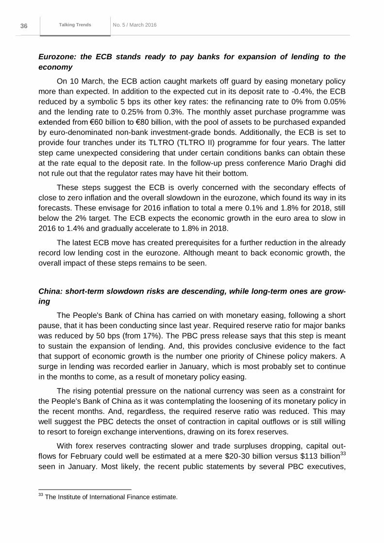
0.5%. The financial market rebound following the slump at the start of the year, core infla-
tion accelerated to the highest value for the period since 2012 (Figure 39), and the fa-
vourable labour market combined to make the case for expectations of tough Fed rhetoric
on its monetary policy direction. To counter these expectations, the Fed's statement was
soft enough and the key rate projection was substantially downgraded.
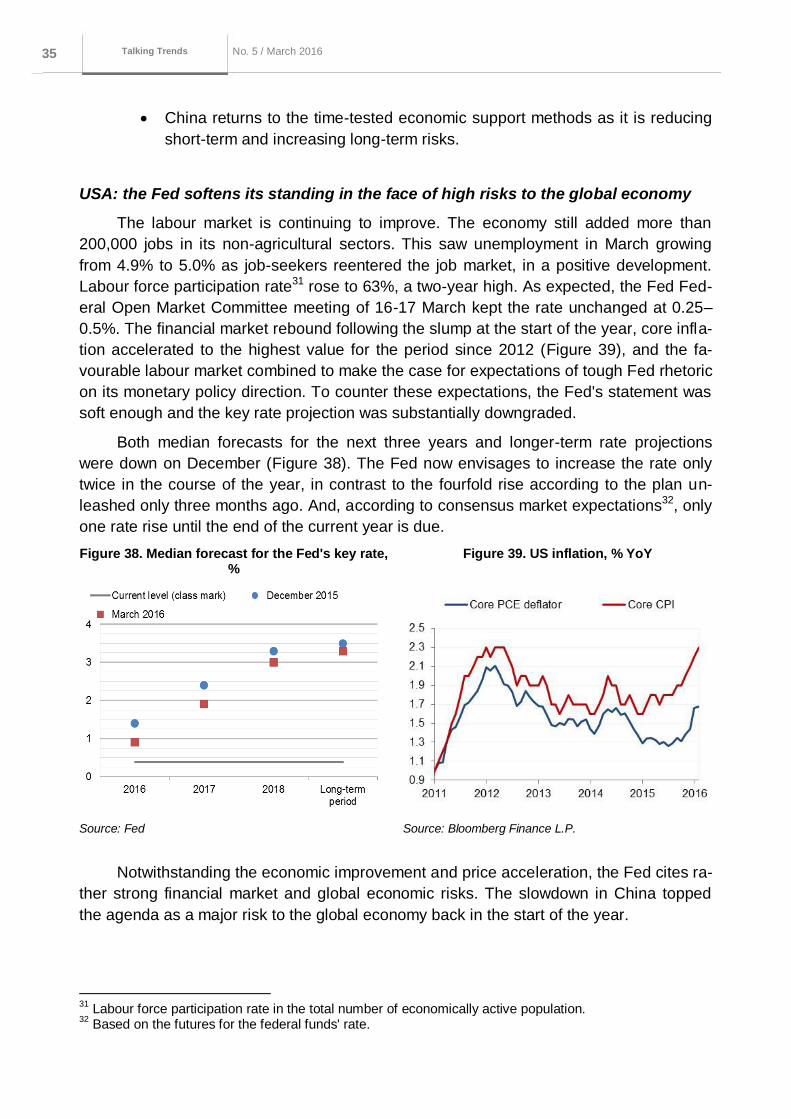
Both median forecasts for the next three years and longer-term rate projections
were down on December (Figure 38). The Fed now envisages to increase the rate only
twice in the course of the year, in contrast to the fourfold rise according to the plan un-
leashed only three months ago. And, according to consensus market expectations32, only
one rate rise until the end of the current year is due.
Figure 38. Median forecast for the Fed's key rate, %
Figure 39. US inflation, % YoY
Source: Fed Source: Bloomberg Finance L.P.
Notwithstanding the economic improvement and price acceleration, the Fed cites ra-
ther strong financial market and global economic risks. The slowdown in China topped
the agenda as a major risk to the global economy back in the start of the year.
31
Labour force participation rate in the total number of economically active population. 32
Based on the futures for the federal funds' rate.
Серия до кла до в о б э ко но мичеСких
иССледо ва ниях 36 No. 5 / March 2016
Macroeconomics and markets No. 1 / October
2015
Talking Trends
Eurozone: the ECB stands ready to pay banks for expansion of lending to the
economy
On 10 March, the ECB action caught markets off guard by easing monetary policy
more than expected. In addition to the expected cut in its deposit rate to -0.4%, the ECB
reduced by a symbolic 5 bps its other key rates: the refinancing rate to 0% from 0.05%
and the lending rate to 0.25% from 0.3%. The monthly asset purchase programme was
extended from €60 billion to €80 billion, with the pool of assets to be purchased expanded
by euro-denominated non-bank investment-grade bonds. Additionally, the ECB is set to
provide four tranches under its TLTRO (TLTRO II) programme for four years. The latter
step came unexpected considering that under certain conditions banks can obtain these
at the rate equal to the deposit rate. In the follow-up press conference Mario Draghi did
not rule out that the regulator rates may have hit their bottom.
These steps suggest the ECB is overly concerned with the secondary effects of
close to zero inflation and the overall slowdown in the eurozone, which found its way in its
forecasts. These envisage for 2016 inflation to total a mere 0.1% and 1.8% for 2018, still
below the 2% target. The ECB expects the economic growth in the euro area to slow in
2016 to 1.4% and gradually accelerate to 1.8% in 2018.
The latest ECB move has created prerequisites for a further reduction in the already
record low lending cost in the eurozone. Although meant to back economic growth, the
overall impact of these steps remains to be seen.
China: short-term slowdown risks are descending, while long-term ones are grow-
ing
The People's Bank of China has carried on with monetary easing, following a short
pause, that it has been conducting since last year. Required reserve ratio for major banks
was reduced by 50 bps (from 17%). The PBC press release says that this step is meant
to sustain the expansion of lending. And, this provides conclusive evidence to the fact
that support of economic growth is the number one priority of Chinese policy makers. A
surge in lending was recorded earlier in January, which is most probably set to continue
in the months to come, as a result of monetary policy easing.
The rising potential pressure on the national currency was seen as a constraint for
the People's Bank of China as it was contemplating the loosening of its monetary policy in
the recent months. And, regardless, the required reserve ratio was reduced. This may
well suggest the PBC detects the onset of contraction in capital outflows or is still willing
to resort to foreign exchange interventions, drawing on its forex reserves.
With forex reserves contracting slower and trade surpluses dropping, capital out-
flows for February could well be estimated at a mere $20-30 billion versus $113 billion33
seen in January. Most likely, the recent public statements by several PBC executives,
33
The Institute of International Finance estimate.
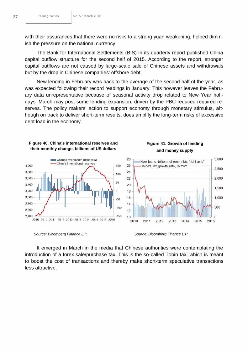
Серия до кла до в о б э ко но мичеСких
иССледо ва ниях 37 No. 5 / March 2016
Macroeconomics and markets No. 1 / October
2015
Talking Trends
with their assurances that there were no risks to a strong yuan weakening, helped dimin-
ish the pressure on the national currency.
The Bank for International Settlements (BIS) in its quarterly report published China
capital outflow structure for the second half of 2015. According to the report, stronger
capital outflows are not caused by large-scale sale of Chinese assets and withdrawals
but by the drop in Chinese companies' offshore debt.
New lending in February was back to the average of the second half of the year, as
was expected following their record readings in January. This however leaves the Febru-
ary data unrepresentative because of seasonal activity drop related to New Year holi-
days. March may post some lending expansion, driven by the PBC-reduced required re-
serves. The policy makers' action to support economy through monetary stimulus, alt-
hough on track to deliver short-term results, does amplify the long-term risks of excessive
debt load in the economy.
Figure 40. China's international reserves and
their monthly change, billions of US dollars
Figure 41. Growth of lending
and money supply
Source: Bloomberg Finance L.P. Source: Bloomberg Finance L.P.
It emerged in March in the media that Chinese authorities were contemplating the
introduction of a forex sale/purchase tax. This is the so-called Tobin tax, which is meant
to boost the cost of transactions and thereby make short-term speculative transactions
less attractive.
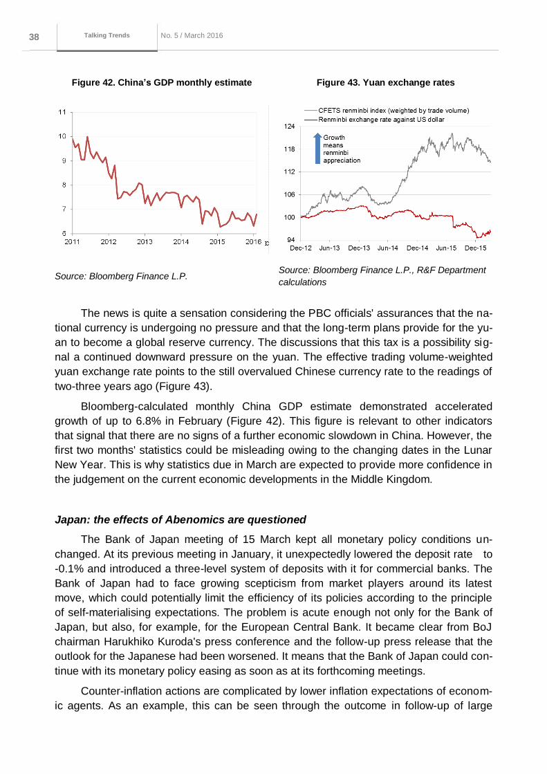
Серия до кла до в о б э ко но мичеСких
иССледо ва ниях 38 No. 5 / March 2016
Macroeconomics and markets No. 1 / October
2015
Talking Trends
Figure 42. China’s GDP monthly estimate Figure 43. Yuan exchange rates
Source: Bloomberg Finance L.P. Source: Bloomberg Finance L.P., R&F Department
calculations
The news is quite a sensation considering the PBC officials' assurances that the na-
tional currency is undergoing no pressure and that the long-term plans provide for the yu-
an to become a global reserve currency. The discussions that this tax is a possibility sig-
nal a continued downward pressure on the yuan. The effective trading volume-weighted
yuan exchange rate points to the still overvalued Chinese currency rate to the readings of
two-three years ago (Figure 43).
Bloomberg-calculated monthly China GDP estimate demonstrated accelerated
growth of up to 6.8% in February (Figure 42). This figure is relevant to other indicators
that signal that there are no signs of a further economic slowdown in China. However, the
first two months' statistics could be misleading owing to the changing dates in the Lunar
New Year. This is why statistics due in March are expected to provide more confidence in
the judgement on the current economic developments in the Middle Kingdom.
Japan: the effects of Abenomics are questioned
The Bank of Japan meeting of 15 March kept all monetary policy conditions un-
changed. At its previous meeting in January, it unexpectedly lowered the deposit rate to
-0.1% and introduced a three-level system of deposits with it for commercial banks. The
Bank of Japan had to face growing scepticism from market players around its latest
move, which could potentially limit the efficiency of its policies according to the principle
of self-materialising expectations. The problem is acute enough not only for the Bank of
Japan, but also, for example, for the European Central Bank. It became clear from BoJ
chairman Harukhiko Kuroda's press conference and the follow-up press release that the
outlook for the Japanese had been worsened. It means that the Bank of Japan could con-
tinue with its monetary policy easing as soon as at its forthcoming meetings.
Counter-inflation actions are complicated by lower inflation expectations of econom-
ic agents. As an example, this can be seen through the outcome in follow-up of large
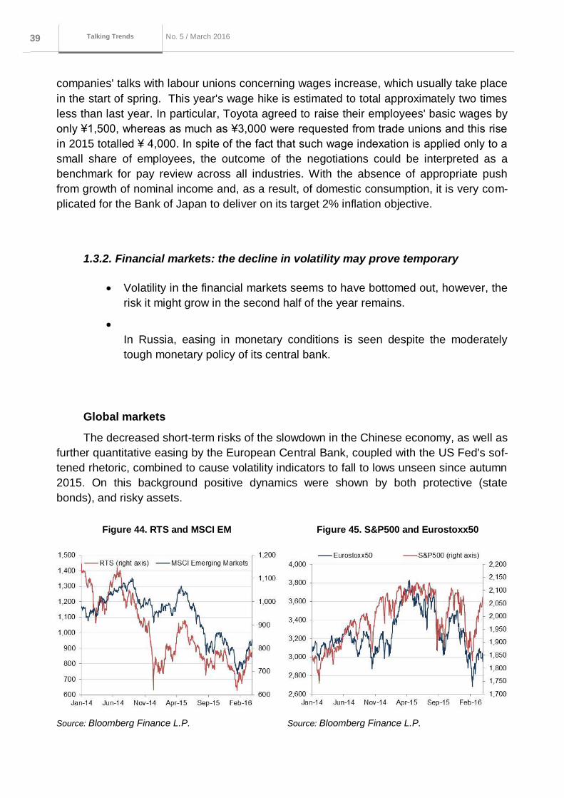
Серия до кла до в о б э ко но мичеСких
иССледо ва ниях 39 No. 5 / March 2016
Macroeconomics and markets No. 1 / October
2015
Talking Trends
companies' talks with labour unions concerning wages increase, which usually take place
in the start of spring. This year's wage hike is estimated to total approximately two times
less than last year. In particular, Toyota agreed to raise their employees' basic wages by
only ¥1,500, whereas as much as ¥3,000 were requested from trade unions and this rise
in 2015 totalled ¥ 4,000. In spite of the fact that such wage indexation is applied only to a
small share of employees, the outcome of the negotiations could be interpreted as a
benchmark for pay review across all industries. With the absence of appropriate push
from growth of nominal income and, as a result, of domestic consumption, it is very com-
plicated for the Bank of Japan to deliver on its target 2% inflation objective.
1.3.2. Financial markets: the decline in volatility may prove temporary
Volatility in the financial markets seems to have bottomed out, however, the
risk it might grow in the second half of the year remains.
In Russia, easing in monetary conditions is seen despite the moderately
tough monetary policy of its central bank.
Global markets
The decreased short-term risks of the slowdown in the Chinese economy, as well as
further quantitative easing by the European Central Bank, coupled with the US Fed's sof-
tened rhetoric, combined to cause volatility indicators to fall to lows unseen since autumn
2015. On this background positive dynamics were shown by both protective (state
bonds), and risky assets.
Figure 44. RTS and MSCI EM Figure 45. S&P500 and Eurostoxx50
Source: Bloomberg Finance L.P. Source: Bloomberg Finance L.P.
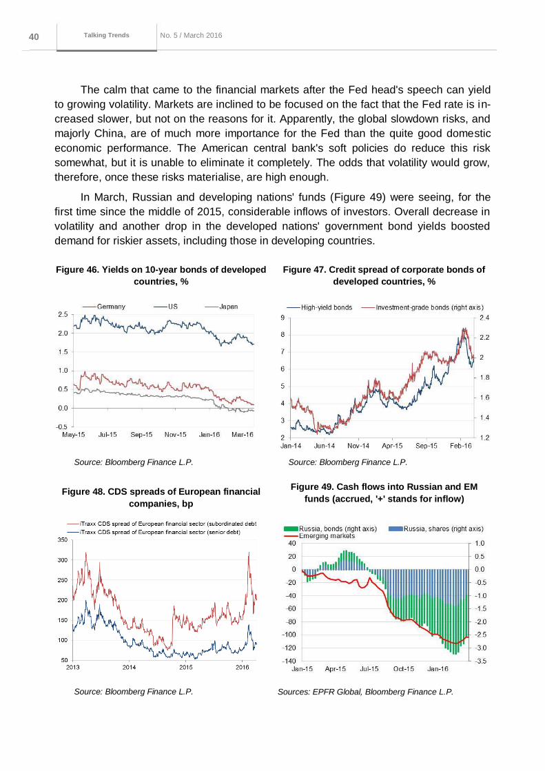
Серия до кла до в о б э ко но мичеСких
иССледо ва ниях 40 No. 5 / March 2016
Macroeconomics and markets No. 1 / October
2015
Talking Trends
The calm that came to the financial markets after the Fed head's speech can yield
to growing volatility. Markets are inclined to be focused on the fact that the Fed rate is in-
creased slower, but not on the reasons for it. Apparently, the global slowdown risks, and
majorly China, are of much more importance for the Fed than the quite good domestic
economic performance. The American central bank's soft policies do reduce this risk
somewhat, but it is unable to eliminate it completely. The odds that volatility would grow,
therefore, once these risks materialise, are high enough.
In March, Russian and developing nations' funds (Figure 49) were seeing, for the
first time since the middle of 2015, considerable inflows of investors. Overall decrease in
volatility and another drop in the developed nations' government bond yields boosted
demand for riskier assets, including those in developing countries.
Figure 46. Yields on 10-year bonds of developed
countries, %
Figure 47. Credit spread of corporate bonds of
developed countries, %
Source: Bloomberg Finance L.P. Source: Bloomberg Finance L.P.
Figure 48. CDS spreads of European financial
companies, bp
Figure 49. Cash flows into Russian and EM
funds (accrued, '+' stands for inflow)
Source: Bloomberg Finance L.P. Sources: EPFR Global, Bloomberg Finance L.P.
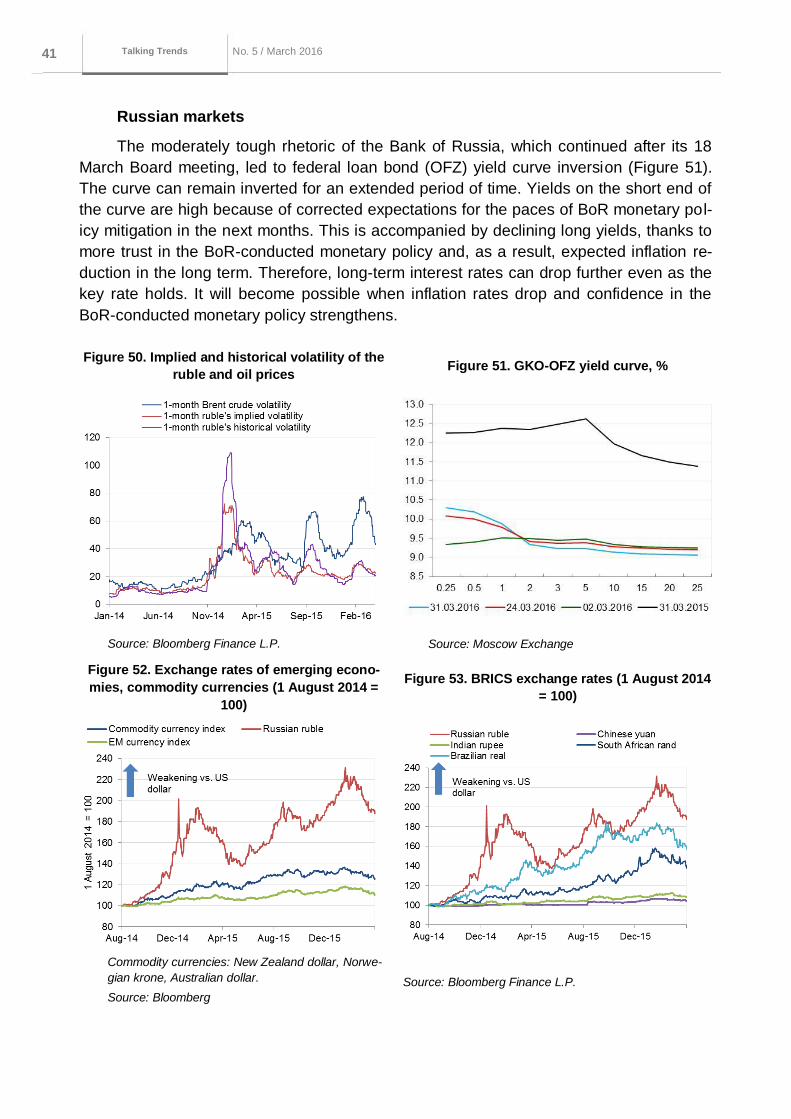
Серия до кла до в о б э ко но мичеСких
иССледо ва ниях 41 No. 5 / March 2016
Macroeconomics and markets No. 1 / October
2015
Talking Trends
Russian markets
The moderately tough rhetoric of the Bank of Russia, which continued after its 18
March Board meeting, led to federal loan bond (OFZ) yield curve inversion (Figure 51).
The curve can remain inverted for an extended period of time. Yields on the short end of
the curve are high because of corrected expectations for the paces of BoR monetary pol-
icy mitigation in the next months. This is accompanied by declining long yields, thanks to
more trust in the BoR-conducted monetary policy and, as a result, expected inflation re-
duction in the long term. Therefore, long-term interest rates can drop further even as the
key rate holds. It will become possible when inflation rates drop and confidence in the
BoR-conducted monetary policy strengthens.
Figure 50. Implied and historical volatility of the
ruble and oil prices Figure 51. GKO-OFZ yield curve, %
Source: Bloomberg Finance L.P. Source: Moscow Exchange
Figure 52. Exchange rates of emerging econo-
mies, commodity currencies (1 August 2014 =
100)
Figure 53. BRICS exchange rates (1 August 2014
= 100)
Commodity currencies: New Zealand dollar, Norwe-
gian krone, Australian dollar.
Source: Bloomberg
Source: Bloomberg Finance L.P.
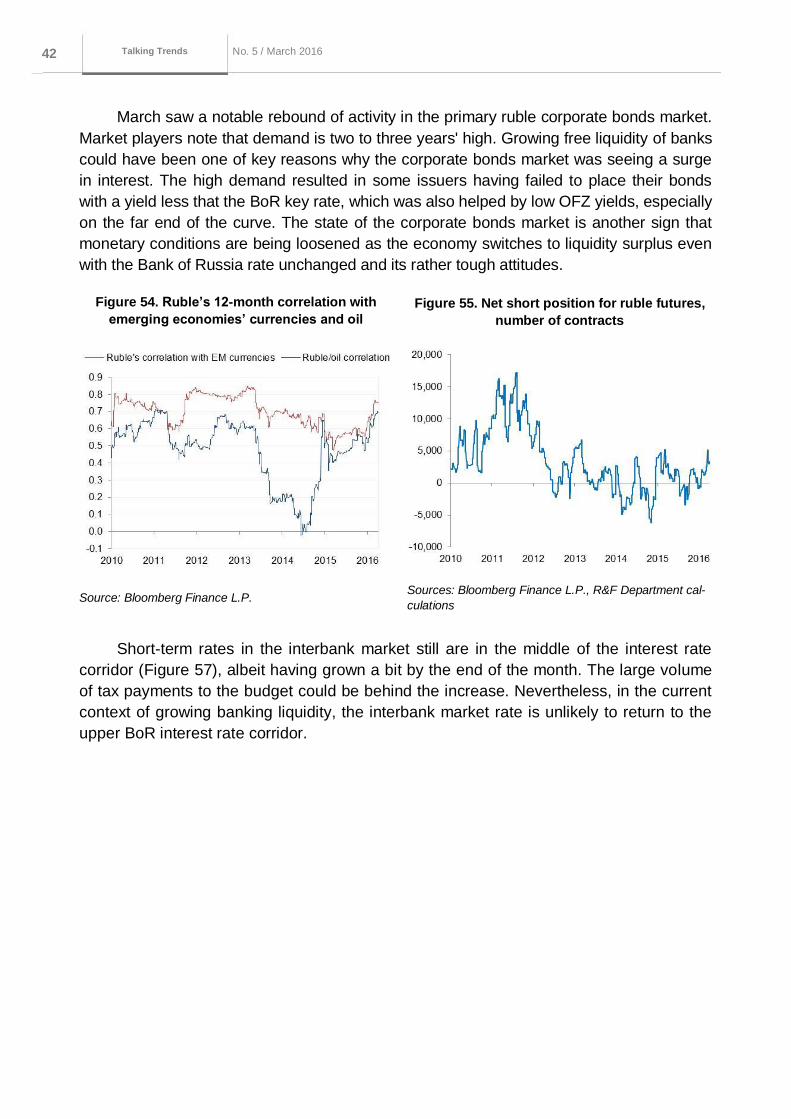
Серия до кла до в о б э ко но мичеСких
иССледо ва ниях 42 No. 5 / March 2016
Macroeconomics and markets No. 1 / October
2015
Talking Trends
March saw a notable rebound of activity in the primary ruble corporate bonds market.
Market players note that demand is two to three years' high. Growing free liquidity of banks
could have been one of key reasons why the corporate bonds market was seeing a surge
in interest. The high demand resulted in some issuers having failed to place their bonds
with a yield less that the BoR key rate, which was also helped by low OFZ yields, especially
on the far end of the curve. The state of the corporate bonds market is another sign that
monetary conditions are being loosened as the economy switches to liquidity surplus even
with the Bank of Russia rate unchanged and its rather tough attitudes.
Figure 54. Ruble’s 12-month correlation with
emerging economies’ currencies and oil
Figure 55. Net short position for ruble futures,
number of contracts
Source: Bloomberg Finance L.P. Sources: Bloomberg Finance L.P., R&F Department cal-
culations
Short-term rates in the interbank market still are in the middle of the interest rate
corridor (Figure 57), albeit having grown a bit by the end of the month. The large volume
of tax payments to the budget could be behind the increase. Nevertheless, in the current
context of growing banking liquidity, the interbank market rate is unlikely to return to the
upper BoR interest rate corridor.
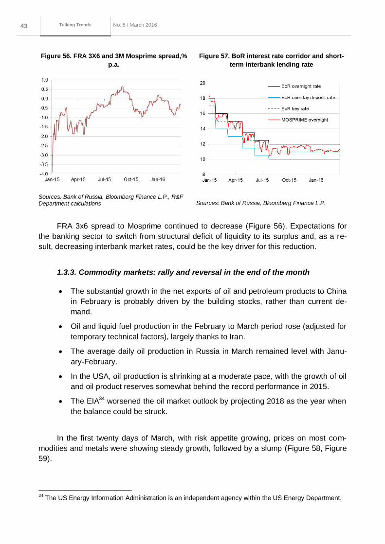
Серия до кла до в о б э ко но мичеСких
иССледо ва ниях 43 No. 5 / March 2016
Macroeconomics and markets No. 1 / October
2015
Talking Trends
Figure 56. FRA 3X6 and 3M Mosprime spread,%
p.a.
Figure 57. BoR interest rate corridor and short-
term interbank lending rate
Sources: Bank of Russia, Bloomberg Finance L.P., R&F Department calculations
Sources: Bank of Russia, Bloomberg Finance L.P.
FRA 3x6 spread to Mosprime continued to decrease (Figure 56). Expectations for
the banking sector to switch from structural deficit of liquidity to its surplus and, as a re-
sult, decreasing interbank market rates, could be the key driver for this reduction.
1.3.3. Commodity markets: rally and reversal in the end of the month
The substantial growth in the net exports of oil and petroleum products to China
in February is probably driven by the building stocks, rather than current de-
mand.
Oil and liquid fuel production in the February to March period rose (adjusted for
temporary technical factors), largely thanks to Iran.
The average daily oil production in Russia in March remained level with Janu-
ary-February.
In the USA, oil production is shrinking at a moderate pace, with the growth of oil
and oil product reserves somewhat behind the record performance in 2015.
The EIA34 worsened the oil market outlook by projecting 2018 as the year when
the balance could be struck.
In the first twenty days of March, with risk appetite growing, prices on most com-
modities and metals were showing steady growth, followed by a slump (Figure 58, Figure
59).
34
The US Energy Information Administration is an independent agency within the US Energy Department.
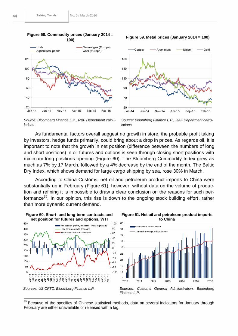
Серия до кла до в о б э ко но мичеСких
иССледо ва ниях 44 No. 5 / March 2016
Macroeconomics and markets No. 1 / October
2015
Talking Trends
Figure 58. Commodity prices (January 2014 =
100) Figure 59. Metal prices (January 2014 = 100)
Source: Bloomberg Finance L.P., R&F Department calcu-
lations
Source: Bloomberg Finance L.P., R&F Department calcu-
lations
As fundamental factors overall suggest no growth in store, the probable profit taking
by investors, hedge funds primarily, could bring about a drop in prices. As regards oil, it is
important to note that the growth in net position (difference between the numbers of long
and short positions) in oil futures and options is seen through closing short positions with
minimum long positions opening (Figure 60). The Bloomberg Commodity Index grew as
much as 7% by 17 March, followed by a 4% decrease by the end of the month. The Baltic
Dry Index, which shows demand for large cargo shipping by sea, rose 30% in March.
According to China Customs, net oil and petroleum product imports to China were
substantially up in February (Figure 61), however, without data on the volume of produc-
tion and refining it is impossible to draw a clear conclusion on the reasons for such per-
formance35. In our opinion, this rise is down to the ongoing stock building effort, rather
than more dynamic current demand.
Figure 60. Short- and long-term contracts and net position for futures and options, WTI
Figure 61. Net oil and petroleum product imports to China
Sources: US CFTC, Bloomberg Finance L.P. Sources: Customs General Administration, Bloomberg Finance L.P.
35
Because of the specifics of Chinese statistical methods, data on several indicators for January through February are either unavailable or released with a lag.
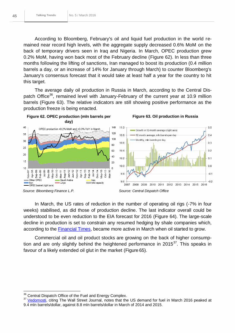
Серия до кла до в о б э ко но мичеСких
иССледо ва ниях 45 No. 5 / March 2016
Macroeconomics and markets No. 1 / October
2015
Talking Trends
According to Bloomberg, February's oil and liquid fuel production in the world re-
mained near record high levels, with the aggregate supply decreased 0.6% MoM on the
back of temporary drivers seen in Iraq and Nigeria. In March, OPEC production grew
0.2% MoM, having won back most of the February decline (Figure 62). In less than three
months following the lifting of sanctions, Iran managed to boost its production (0.4 million
barrels a day, or an increase of 14% for January through March) to counter Bloomberg's
January's consensus forecast that it would take at least half a year for the country to hit
this target.
The average daily oil production in Russia in March, according to the Central Dis-
patch Office36, remained level with January-February of the current year at 10.9 million
barrels (Figure 63). The relative indicators are still showing positive performance as the
production freeze is being enacted.
Figure 62. OPEC production (mln barrels per
day)
Figure 63. Oil production in Russia
Source: Bloomberg Finance L.P. Source: Central Dispatch Office
In March, the US rates of reduction in the number of operating oil rigs (-7% in four
weeks) stabilised, as did those of production decline. The last indicator overall could be
understood to be even reduction to the EIA forecast for 2016 (Figure 64). The large-scale
decline in production is set to constrain any resumed hedging by shale companies which,
according to the Financial Times, became more active in March when oil started to grow.
Commercial oil and oil product stocks are growing on the back of higher consump-
tion and are only slightly behind the heightened performance in 201537. This speaks in
favour of a likely extended oil glut in the market (Figure 65).
36
Central Dispatch Office of the Fuel and Energy Complex. 37
Vedomosti, citing The Wall Street Journal, notes that the US demand for fuel in March 2016 peaked at 9.4 mln barrels/dollar, against 8.8 mln barrels/dollar in March of 2014 and 2015.
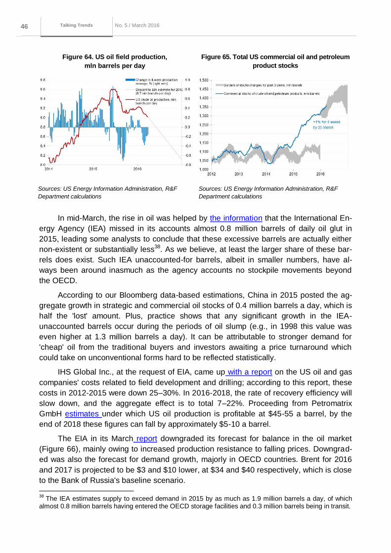
Серия до кла до в о б э ко но мичеСких
иССледо ва ниях 46 No. 5 / March 2016
Macroeconomics and markets No. 1 / October
2015
Talking Trends
Figure 64. US oil field production,
mln barrels per day
Figure 65. Total US commercial oil and petroleum
product stocks
Sources: US Energy Information Administration, R&F
Department calculations
Sources: US Energy Information Administration, R&F
Department calculations
In mid-March, the rise in oil was helped by the information that the International En-
ergy Agency (IEA) missed in its accounts almost 0.8 million barrels of daily oil glut in
2015, leading some analysts to conclude that these excessive barrels are actually either
non-existent or substantially less38. As we believe, at least the larger share of these bar-
rels does exist. Such IEA unaccounted-for barrels, albeit in smaller numbers, have al-
ways been around inasmuch as the agency accounts no stockpile movements beyond
the OECD.
According to our Bloomberg data-based estimations, China in 2015 posted the ag-
gregate growth in strategic and commercial oil stocks of 0.4 million barrels a day, which is
half the 'lost' amount. Plus, practice shows that any significant growth in the IEA-
unaccounted barrels occur during the periods of oil slump (e.g., in 1998 this value was
even higher at 1.3 million barrels a day). It can be attributable to stronger demand for
'cheap' oil from the traditional buyers and investors awaiting a price turnaround which
could take on unconventional forms hard to be reflected statistically.
IHS Global Inc., at the request of EIA, came up with a report on the US oil and gas
companies' costs related to field development and drilling; according to this report, these
costs in 2012-2015 were down 25–30%. In 2016-2018, the rate of recovery efficiency will
slow down, and the aggregate effect is to total 7–22%. Proceeding from Petromatrix
GmbH estimates under which US oil production is profitable at $45-55 a barrel, by the
end of 2018 these figures can fall by approximately $5-10 a barrel.
The EIA in its March report downgraded its forecast for balance in the oil market
(Figure 66), mainly owing to increased production resistance to falling prices. Downgrad-
ed was also the forecast for demand growth, majorly in OECD countries. Brent for 2016
and 2017 is projected to be $3 and $10 lower, at $34 and $40 respectively, which is close
to the Bank of Russia's baseline scenario.
38
The IEA estimates supply to exceed demand in 2015 by as much as 1.9 million barrels a day, of which almost 0.8 million barrels having entered the OECD storage facilities and 0.3 million barrels being in transit.
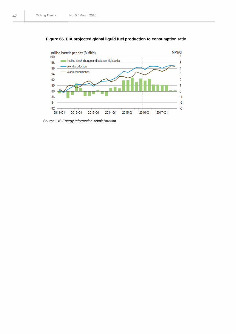
Серия до кла до в о б э ко но мичеСких
иССледо ва ниях 47 No. 5 / March 2016
Macroeconomics and markets No. 1 / October
2015
Talking Trends
Figure 66. EIA projected global liquid fuel production to consumption ratio
Source: US Energy Information Administration
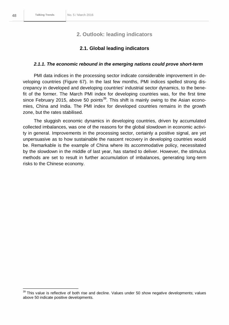
Серия до кла до в о б э ко но мичеСких
иССледо ва ниях 48 No. 5 / March 2016
Macroeconomics and markets No. 1 / October
2015
Talking Trends
2. Outlook: leading indicators
2.1. Global leading indicators
2.1.1. The economic rebound in the emerging nations could prove short-term
PMI data indices in the processing sector indicate considerable improvement in de-
veloping countries (Figure 67). In the last few months, PMI indices spelled strong dis-
crepancy in developed and developing countries' industrial sector dynamics, to the bene-
fit of the former. The March PMI index for developing countries was, for the first time
since February 2015, above 50 points39. This shift is mainly owing to the Asian econo-
mies, China and India. The PMI index for developed countries remains in the growth
zone, but the rates stabilised.
The sluggish economic dynamics in developing countries, driven by accumulated
collected imbalances, was one of the reasons for the global slowdown in economic activi-
ty in general. Improvements in the processing sector, certainly a positive signal, are yet
unpersuasive as to how sustainable the nascent recovery in developing countries would
be. Remarkable is the example of China where its accommodative policy, necessitated
by the slowdown in the middle of last year, has started to deliver. However, the stimulus
methods are set to result in further accumulation of imbalances, generating long-term
risks to the Chinese economy.
39
This value is reflective of both rise and decline. Values under 50 show negative developments; values above 50 indicate positive developments.
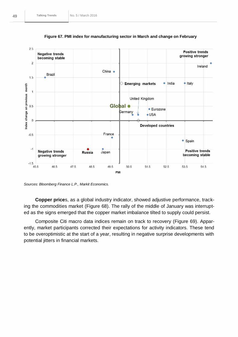
Серия до кла до в о б э ко но мичеСких
иССледо ва ниях 49 No. 5 / March 2016
Macroeconomics and markets No. 1 / October
2015
Talking Trends
Figure 67. PMI index for manufacturing sector in March and change on February
Sources: Bloomberg Finance L.P., Markit Economics.
Copper prices, as a global industry indicator, showed adjustive performance, track-
ing the commodities market (Figure 68). The rally of the middle of January was interrupt-
ed as the signs emerged that the copper market imbalance tilted to supply could persist.
Composite Citi macro data indices remain on track to recovery (Figure 69). Appar-
ently, market participants corrected their expectations for activity indicators. These tend
to be overoptimistic at the start of a year, resulting in negative surprise developments with
potential jitters in financial markets.
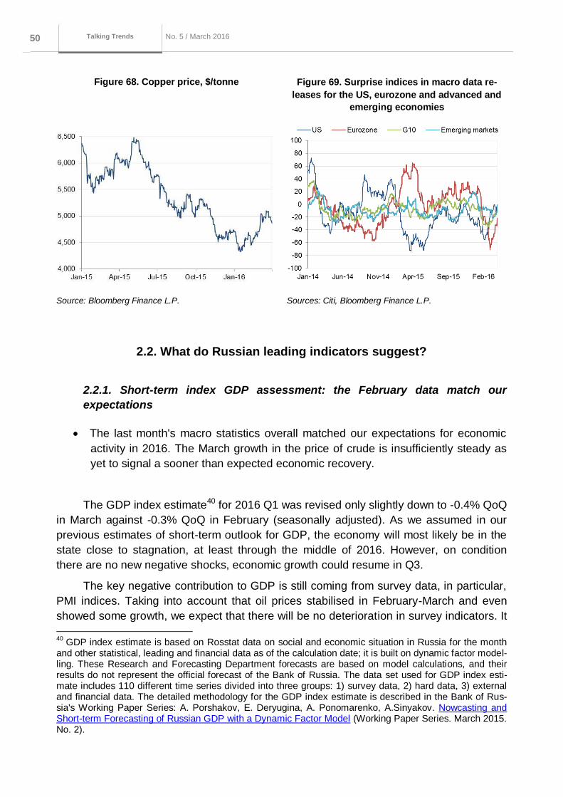
Серия до кла до в о б э ко но мичеСких
иССледо ва ниях 50 No. 5 / March 2016
Macroeconomics and markets No. 1 / October
2015
Talking Trends
Figure 68. Copper price, $/tonne Figure 69. Surprise indices in macro data re-
leases for the US, eurozone and advanced and
emerging economies
Source: Bloomberg Finance L.P. Sources: Citi, Bloomberg Finance L.P.
2.2. What do Russian leading indicators suggest?
2.2.1. Short-term index GDP assessment: the February data match our
expectations
The last month's macro statistics overall matched our expectations for economic
activity in 2016. The March growth in the price of crude is insufficiently steady as
yet to signal a sooner than expected economic recovery.
The GDP index estimate40 for 2016 Q1 was revised only slightly down to -0.4% QoQ
in March against -0.3% QoQ in February (seasonally adjusted). As we assumed in our
previous estimates of short-term outlook for GDP, the economy will most likely be in the
state close to stagnation, at least through the middle of 2016. However, on condition
there are no new negative shocks, economic growth could resume in Q3.
The key negative contribution to GDP is still coming from survey data, in particular,
PMI indices. Taking into account that oil prices stabilised in February-March and even
showed some growth, we expect that there will be no deterioration in survey indicators. It
40
GDP index estimate is based on Rosstat data on social and economic situation in Russia for the month and other statistical, leading and financial data as of the calculation date; it is built on dynamic factor model-ling. These Research and Forecasting Department forecasts are based on model calculations, and their results do not represent the official forecast of the Bank of Russia. The data set used for GDP index esti-mate includes 110 different time series divided into three groups: 1) survey data, 2) hard data, 3) external and financial data. The detailed methodology for the GDP index estimate is described in the Bank of Rus-sia's Working Paper Series: A. Porshakov, E. Deryugina, A. Ponomarenko, A.Sinyakov. Nowcasting and Short-term Forecasting of Russian GDP with a Dynamic Factor Model (Working Paper Series. March 2015. No. 2).
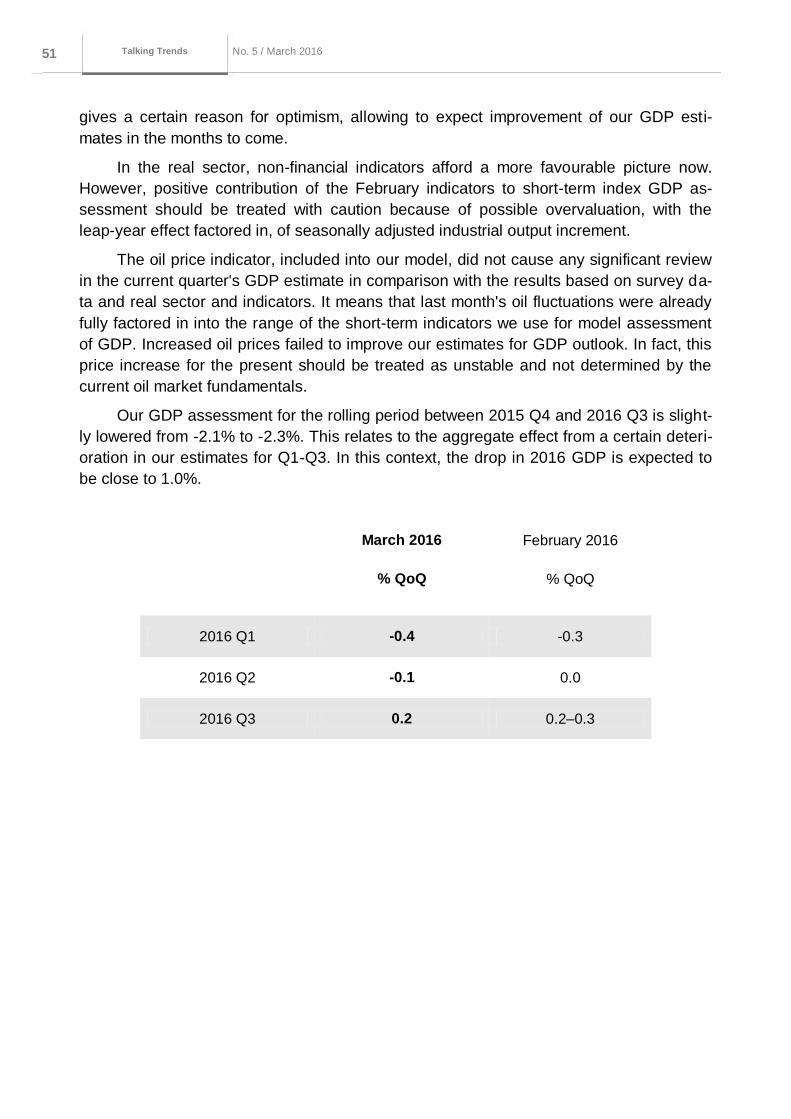
Серия до кла до в о б э ко но мичеСких
иССледо ва ниях 51 No. 5 / March 2016
Macroeconomics and markets No. 1 / October
2015
Talking Trends
gives a certain reason for optimism, allowing to expect improvement of our GDP esti-
mates in the months to come.
In the real sector, non-financial indicators afford a more favourable picture now.
However, positive contribution of the February indicators to short-term index GDP as-
sessment should be treated with caution because of possible overvaluation, with the
leap-year effect factored in, of seasonally adjusted industrial output increment.
The oil price indicator, included into our model, did not cause any significant review
in the current quarter's GDP estimate in comparison with the results based on survey da-
ta and real sector and indicators. It means that last month's oil fluctuations were already
fully factored in into the range of the short-term indicators we use for model assessment
of GDP. Increased oil prices failed to improve our estimates for GDP outlook. In fact, this
price increase for the present should be treated as unstable and not determined by the
current oil market fundamentals.
Our GDP assessment for the rolling period between 2015 Q4 and 2016 Q3 is slight-
ly lowered from -2.1% to -2.3%. This relates to the aggregate effect from a certain deteri-
oration in our estimates for Q1-Q3. In this context, the drop in 2016 GDP is expected to
be close to 1.0%.
March 2016 February 2016
% QoQ
% QoQ
2016 Q1 -0.4 -0.3
2016 Q2 -0.1 0.0
2016 Q3 0.2 0.2–0.3
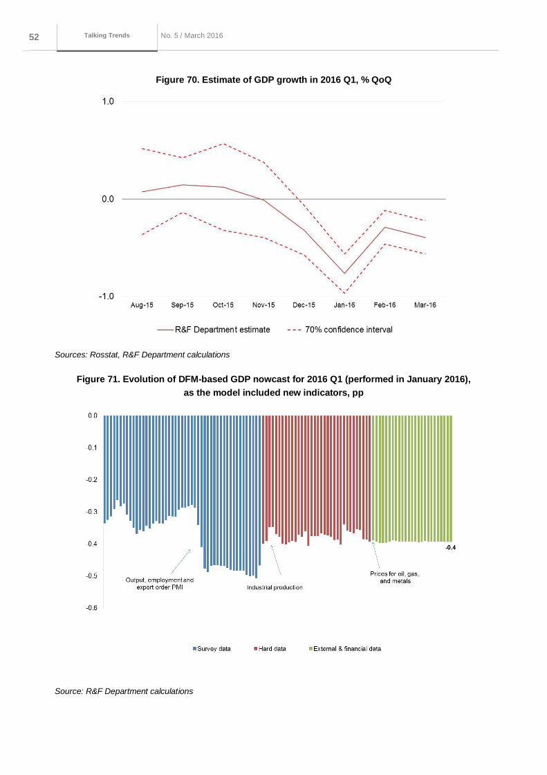
Серия до кла до в о б э ко но мичеСких
иССледо ва ниях 52 No. 5 / March 2016
Macroeconomics and markets No. 1 / October
2015
Talking Trends
Figure 70. Estimate of GDP growth in 2016 Q1, % QoQ
Sources: Rosstat, R&F Department calculations
Figure 71. Evolution of DFM-based GDP nowcast for 2016 Q1 (performed in January 2016),
as the model included new indicators, pp
Source: R&F Department calculations
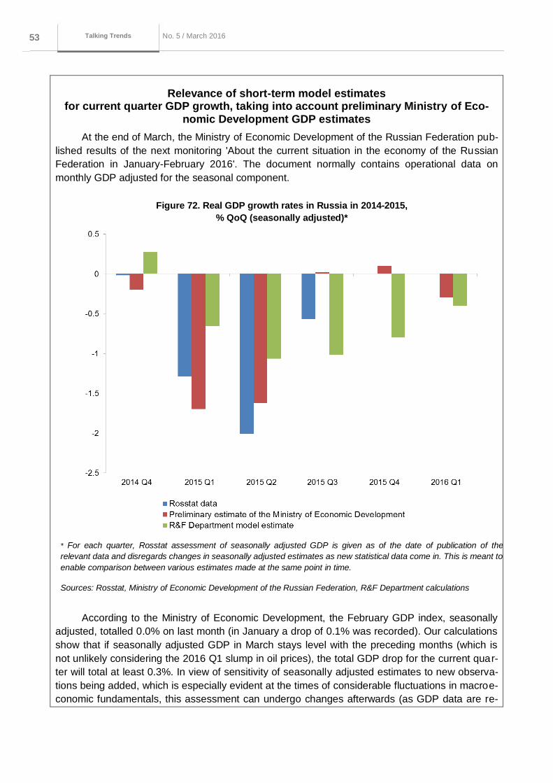
Серия до кла до в о б э ко но мичеСких
иССледо ва ниях 53 No. 5 / March 2016
Macroeconomics and markets No. 1 / October
2015
Talking Trends
Relevance of short-term model estimates for current quarter GDP growth, taking into account preliminary Ministry of Eco-
nomic Development GDP estimates
At the end of March, the Ministry of Economic Development of the Russian Federation pub-
lished results of the next monitoring 'About the current situation in the economy of the Russian
Federation in January-February 2016'. The document normally contains operational data on
monthly GDP adjusted for the seasonal component.
Figure 72. Real GDP growth rates in Russia in 2014-2015,
% QoQ (seasonally adjusted)*
* For each quarter, Rosstat assessment of seasonally adjusted GDP is given as of the date of publication of the
relevant data and disregards changes in seasonally adjusted estimates as new statistical data come in. This is meant to
enable comparison between various estimates made at the same point in time.
Sources: Rosstat, Ministry of Economic Development of the Russian Federation, R&F Department calculations
According to the Ministry of Economic Development, the February GDP index, seasonally
adjusted, totalled 0.0% on last month (in January a drop of 0.1% was recorded). Our calculations
show that if seasonally adjusted GDP in March stays level with the preceding months (which is
not unlikely considering the 2016 Q1 slump in oil prices), the total GDP drop for the current quar-
ter will total at least 0.3%. In view of sensitivity of seasonally adjusted estimates to new observa-
tions being added, which is especially evident at the times of considerable fluctuations in macroe-
conomic fundamentals, this assessment can undergo changes afterwards (as GDP data are re-

Серия до кла до в о б э ко но мичеСких
иССледо ва ниях 54 No. 5 / March 2016
Macroeconomics and markets No. 1 / October
2015
Talking Trends
leased for the quarters that follow).
It is also necessary to consider that the Ministry of Economic Development estimates of
monthly GDP are tentative and could be put under reviews, deviating, as a result, from GDP es-
timates by Rosstat. This is especially clear from the discrepancy between the tentative data of the
Ministry of Economic Development and final Rosstat estimates for the last quarters (Figure 72).
Therefore, the short-term model GDP estimates for the current quarter made even after its expiry
(but in anticipation of Rosstat data), can exceed Ministry of Economic Development estimates in
terms of accuracy and therefore remain relevant.
2.2.2. Leading business indicator: mixed signals
The assessment of the composite leading business indicator as of early April indi-
cated a slight improvement on the previous results obtained two weeks earlier (Figure
73). The positive review of our estimates stems from the data on REB diffusion indices
which indicated a notable growth in March of enterprises with a better output and em-
ployment, and also a number of the PMI indices in processing for March in the part of
complete production and new export orders.
Although statistics on separate PMI indices remain rather weak, last month saw a
stop in the descent of PMI indices marked by leading qualities more than others.
Figure 73. The cyclical component of industrial production
(January 2015 = 100, seasonally adjusted) and leading business index
Sources: Rosstat, HSBC, Russian Economic Barometer, R&F Department calculations

Серия до кла до в о б э ко но мичеСких
иССледо ва ниях 55 No. 5 / March 2016
Macroeconomics and markets No. 1 / October
2015
Talking Trends
2.2.3. Financial analysts' forecasts
1) GDP
Bloomberg consensus forecast data of as of March 31 show that most of analysts
kept their earlier estimates for 2016 GDP growth. The forecast was reviewed, if at all,
only upwards: a month earlier, most of respondents expected annual GDP to drop 1.3–
1.5%, while as of the end of March surveys showed prevailing expectations for a lighter
recession at 1.0% (Figure 74).
Improvement in some analysts' forecasts came in on the back of rising oil in March,
as well as the positive production statistics in manufacturing in February. Our index GDP
assessment (see Section 2.2.1) for 2016 in general matches analysts' consensus
forecast.
Figure 74. GDP growth forecasts by external
analysts in 2016
Figure 75. Consumer inflation forecasts by
external analysts in 2016, % YoY, annual
average
Sources: Bloomberg Finance L.P., R&F Department cal-
culations
Sources: Bloomberg Finance L.P., R&F Department cal-
culations
2) Inflation
The actual average 2016 median forecast for consumer inflation based on February
readings fell from 8.6% in February to 8.3% in March, triggered by the slowdown over the
past weeks (Figure 75). There was more density in 2016 inflation forecasts for the last
month, in a sign of decreased uncertainty as to the economic situation as oil was showing
positive performance and the ruble strengthened in March.
3) Bank of Russia monetary policy
Expectations of Bloomberg analysts for the Bank of Russia key rate for the end of
2016 are 9.5% (Figure76). The median rate forecast therefore has remained unchanged
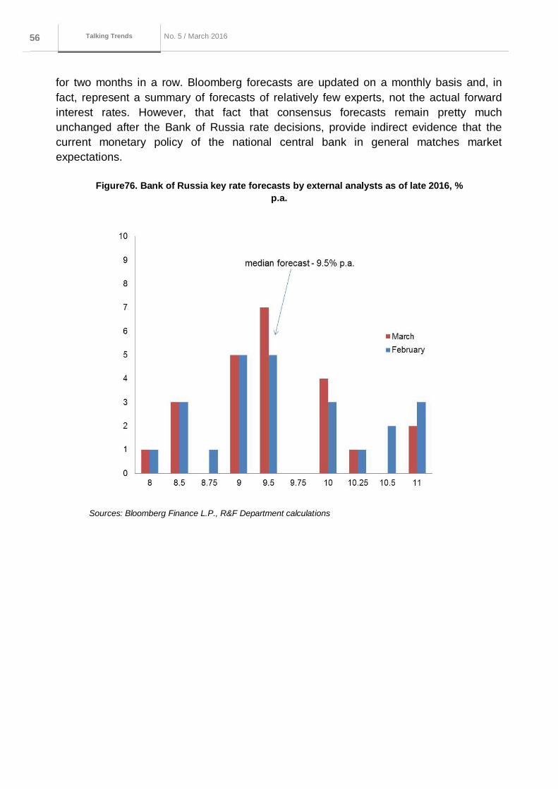
Серия до кла до в о б э ко но мичеСких
иССледо ва ниях 56 No. 5 / March 2016
Macroeconomics and markets No. 1 / October
2015
Talking Trends
for two months in a row. Bloomberg forecasts are updated on a monthly basis and, in
fact, represent a summary of forecasts of relatively few experts, not the actual forward
interest rates. However, that fact that consensus forecasts remain pretty much
unchanged after the Bank of Russia rate decisions, provide indirect evidence that the
current monetary policy of the national central bank in general matches market
expectations.
Figure76. Bank of Russia key rate forecasts by external analysts as of late 2016, %
p.a.
Sources: Bloomberg Finance L.P., R&F Department calculations
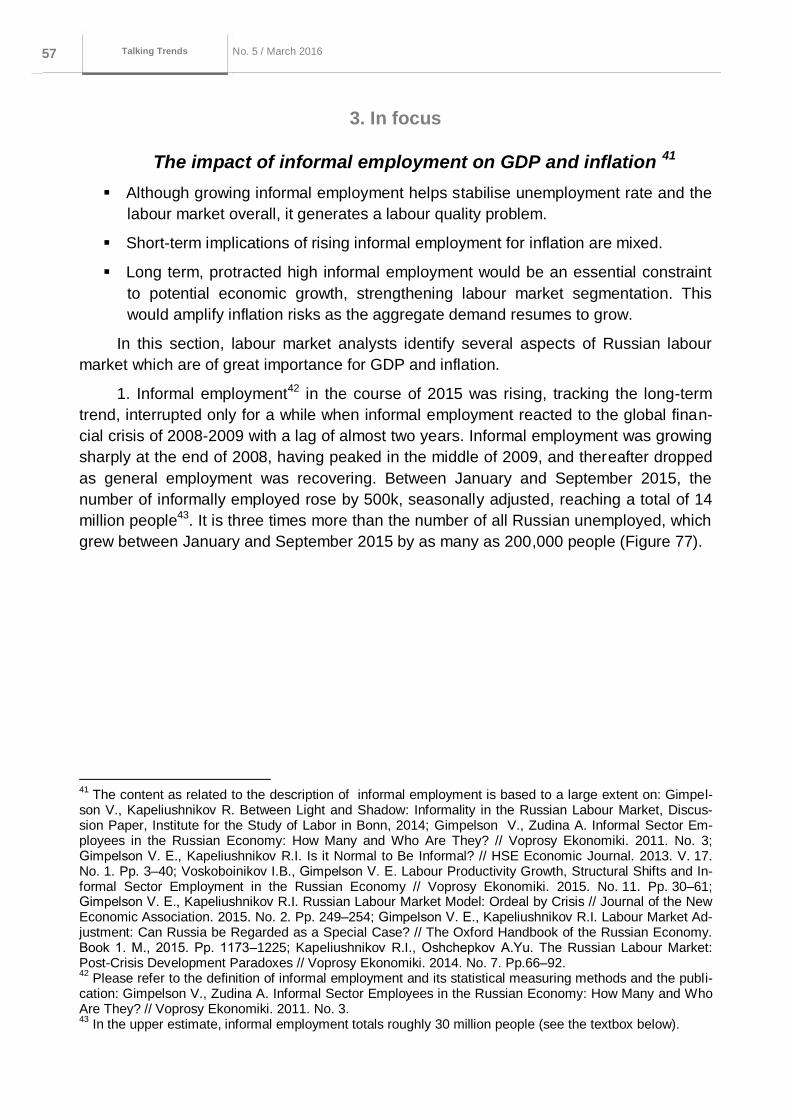
Серия до кла до в о б э ко но мичеСких
иССледо ва ниях 57 No. 5 / March 2016
Macroeconomics and markets No. 1 / October
2015
Talking Trends
3. In focus
The impact of informal employment on GDP and inflation 41
Although growing informal employment helps stabilise unemployment rate and the
labour market overall, it generates a labour quality problem.
Short-term implications of rising informal employment for inflation are mixed.
Long term, protracted high informal employment would be an essential constraint
to potential economic growth, strengthening labour market segmentation. This
would amplify inflation risks as the aggregate demand resumes to grow.
In this section, labour market analysts identify several aspects of Russian labour
market which are of great importance for GDP and inflation.
1. Informal employment42 in the course of 2015 was rising, tracking the long-term
trend, interrupted only for a while when informal employment reacted to the global finan-
cial crisis of 2008-2009 with a lag of almost two years. Informal employment was growing
sharply at the end of 2008, having peaked in the middle of 2009, and thereafter dropped
as general employment was recovering. Between January and September 2015, the
number of informally employed rose by 500k, seasonally adjusted, reaching a total of 14
million people43. It is three times more than the number of all Russian unemployed, which
grew between January and September 2015 by as many as 200,000 people (Figure 77).
41
The content as related to the description of informal employment is based to a large extent on: Gimpel-son V., Kapeliushnikov R. Between Light and Shadow: Informality in the Russian Labour Market, Discus-sion Paper, Institute for the Study of Labor in Bonn, 2014; Gimpelson V., Zudina A. Informal Sector Em-ployees in the Russian Economy: How Many and Who Are They? // Voprosy Ekonomiki. 2011. No. 3; Gimpelson V. Е., Kapeliushnikov R.I. Is it Normal to Be Informal? // HSE Economic Journal. 2013. V. 17. No. 1. Pp. 3–40; Voskoboinikov I.B., Gimpelson V. Е. Labour Productivity Growth, Structural Shifts and In-formal Sector Employment in the Russian Economy // Voprosy Ekonomiki. 2015. No. 11. Pp. 30–61; Gimpelson V. Е., Kapeliushnikov R.I. Russian Labour Market Model: Ordeal by Crisis // Journal of the New Economic Association. 2015. No. 2. Pp. 249–254; Gimpelson V. Е., Kapeliushnikov R.I. Labour Market Ad-justment: Can Russia be Regarded as a Special Case? // The Oxford Handbook of the Russian Economy. Book 1. М., 2015. Pp. 1173–1225; Kapeliushnikov R.I., Oshchepkov А.Yu. The Russian Labour Market: Post-Crisis Development Paradoxes // Voprosy Ekonomiki. 2014. No. 7. Pp.66–92. 42
Please refer to the definition of informal employment and its statistical measuring methods and the publi-cation: Gimpelson V., Zudina A. Informal Sector Employees in the Russian Economy: How Many and Who Are They? // Voprosy Ekonomiki. 2011. No. 3. 43
In the upper estimate, informal employment totals roughly 30 million people (see the textbox below).
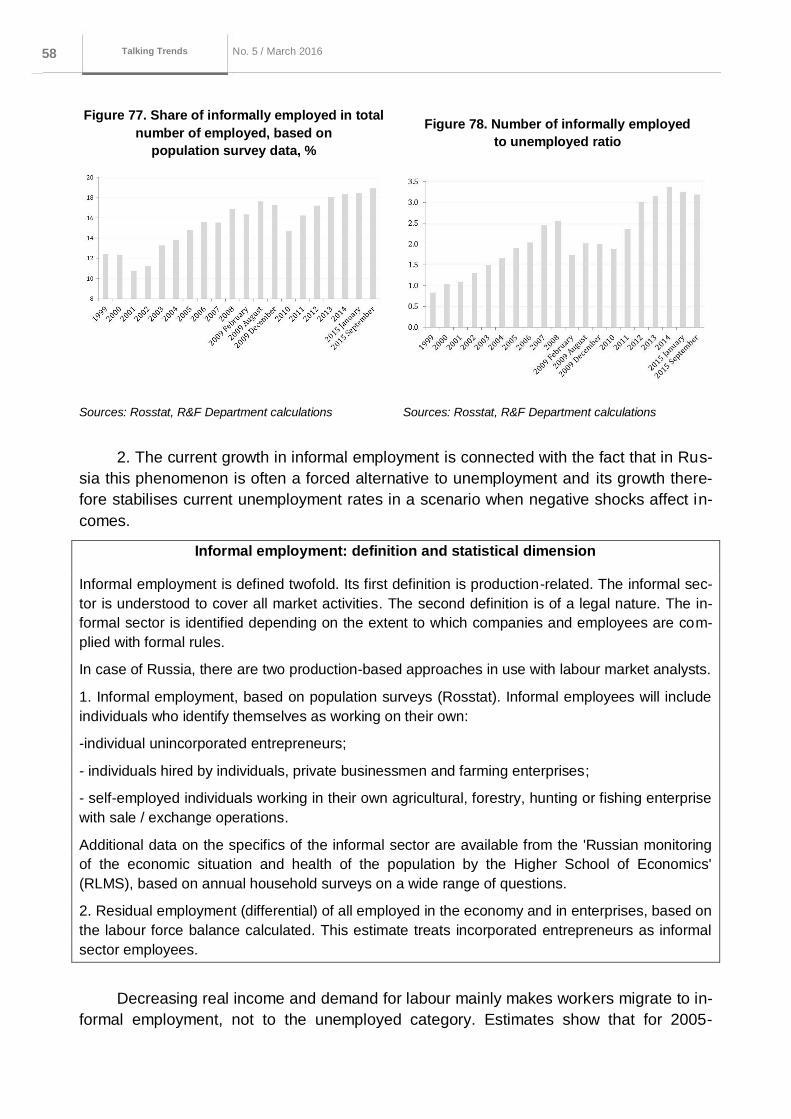
Серия до кла до в о б э ко но мичеСких
иССледо ва ниях 58 No. 5 / March 2016
Macroeconomics and markets No. 1 / October
2015
Talking Trends
Figure 77. Share of informally employed in total
number of employed, based on
population survey data, %
Figure 78. Number of informally employed
to unemployed ratio
Sources: Rosstat, R&F Department calculations Sources: Rosstat, R&F Department calculations
2. The current growth in informal employment is connected with the fact that in Rus-
sia this phenomenon is often a forced alternative to unemployment and its growth there-
fore stabilises current unemployment rates in a scenario when negative shocks affect in-
comes.
Informal employment: definition and statistical dimension
Informal employment is defined twofold. Its first definition is production-related. The informal sec-
tor is understood to cover all market activities. The second definition is of a legal nature. The in-
formal sector is identified depending on the extent to which companies and employees are com-
plied with formal rules.
In case of Russia, there are two production-based approaches in use with labour market analysts.
1. Informal employment, based on population surveys (Rosstat). Informal employees will include
individuals who identify themselves as working on their own:
-individual unincorporated entrepreneurs;
- individuals hired by individuals, private businessmen and farming enterprises;
- self-employed individuals working in their own agricultural, forestry, hunting or fishing enterprise
with sale / exchange operations.
Additional data on the specifics of the informal sector are available from the 'Russian monitoring
of the economic situation and health of the population by the Higher School of Economics'
(RLMS), based on annual household surveys on a wide range of questions.
2. Residual employment (differential) of all employed in the economy and in enterprises, based on
the labour force balance calculated. This estimate treats incorporated entrepreneurs as informal
sector employees.
Decreasing real income and demand for labour mainly makes workers migrate to in-
formal employment, not to the unemployed category. Estimates show that for 2005-
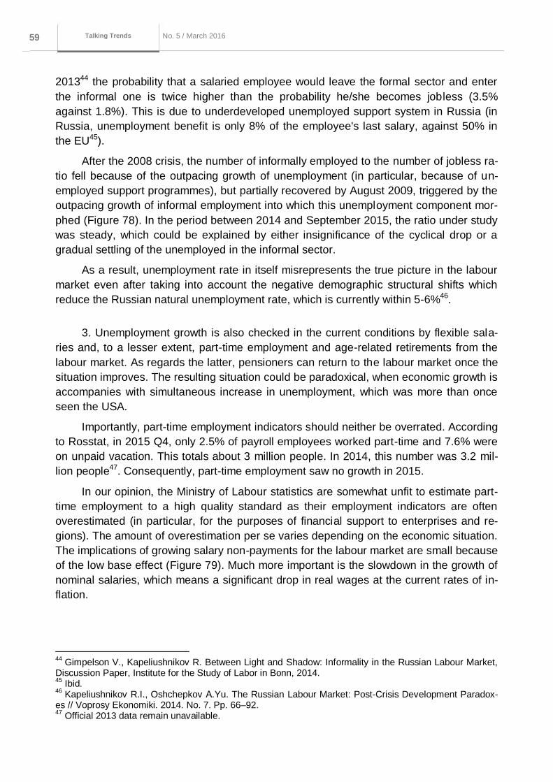
Серия до кла до в о б э ко но мичеСких
иССледо ва ниях 59 No. 5 / March 2016
Macroeconomics and markets No. 1 / October
2015
Talking Trends
201344 the probability that a salaried employee would leave the formal sector and enter
the informal one is twice higher than the probability he/she becomes jobless (3.5%
against 1.8%). This is due to underdeveloped unemployed support system in Russia (in
Russia, unemployment benefit is only 8% of the employee's last salary, against 50% in
the EU45).
After the 2008 crisis, the number of informally employed to the number of jobless ra-
tio fell because of the outpacing growth of unemployment (in particular, because of un-
employed support programmes), but partially recovered by August 2009, triggered by the
outpacing growth of informal employment into which this unemployment component mor-
phed (Figure 78). In the period between 2014 and September 2015, the ratio under study
was steady, which could be explained by either insignificance of the cyclical drop or a
gradual settling of the unemployed in the informal sector.
As a result, unemployment rate in itself misrepresents the true picture in the labour
market even after taking into account the negative demographic structural shifts which
reduce the Russian natural unemployment rate, which is currently within 5-6%46.
3. Unemployment growth is also checked in the current conditions by flexible sala-
ries and, to a lesser extent, part-time employment and age-related retirements from the
labour market. As regards the latter, pensioners can return to the labour market once the
situation improves. The resulting situation could be paradoxical, when economic growth is
accompanies with simultaneous increase in unemployment, which was more than once
seen the USA.
Importantly, part-time employment indicators should neither be overrated. According
to Rosstat, in 2015 Q4, only 2.5% of payroll employees worked part-time and 7.6% were
on unpaid vacation. This totals about 3 million people. In 2014, this number was 3.2 mil-
lion people47. Consequently, part-time employment saw no growth in 2015.
In our opinion, the Ministry of Labour statistics are somewhat unfit to estimate part-
time employment to a high quality standard as their employment indicators are often
overestimated (in particular, for the purposes of financial support to enterprises and re-
gions). The amount of overestimation per se varies depending on the economic situation.
The implications of growing salary non-payments for the labour market are small because
of the low base effect (Figure 79). Much more important is the slowdown in the growth of
nominal salaries, which means a significant drop in real wages at the current rates of in-
flation.
44
Gimpelson V., Kapeliushnikov R. Between Light and Shadow: Informality in the Russian Labour Market, Discussion Paper, Institute for the Study of Labor in Bonn, 2014. 45
Ibid. 46
Kapeliushnikov R.I., Oshchepkov А.Yu. The Russian Labour Market: Post-Crisis Development Paradox-es // Voprosy Ekonomiki. 2014. No. 7. Pp. 66–92. 47
Official 2013 data remain unavailable.

Серия до кла до в о б э ко но мичеСких
иССледо ва ниях 60 No. 5 / March 2016
Macroeconomics and markets No. 1 / October
2015
Talking Trends
Figure 79. Overdue wage arrears in January 2006 prices, billions of rubles
0
1
2
3
4
5
6
7
8
2006 2007 2008 2009 2010 2011 2012 2013 2014 2015
Source: Rosstat
4. The second key growth driver for informal employment is the low pace of new job
creation in the formal sector. Some workers will potentially agree to leave the informal
sector but are unable to as the rates of new job creation are weak. For economic restruc-
turing in the aftermath of the recent weakening of the ruble and decreased real wages,
the economy should add jobs at faster rates.
In Russia, the new jobs to occupied jobs ratio remains low. For an example, the av-
erage business cycle job creation ratio in the USA and Europe is about 15%. In Russia,
this ratio in 2014 was on the order of 10%. It probably remained flat for 2015, despite the
fact that the economy was faced up with a structural shift, not a business cycle.
5. Informal employment (hidden unemployment) occurs in the non-tradables sector
(unexposed to import substitution), that is, we are seeing inter-segmental migrations
(formal and informal) in one industry. Non-tradables sector activities are marked by lower
labor productivity. Estimates show48 that in Russia migration to informal employment
leads to decreased aggregate labour productivity (or at least its slowdown). Therefore,
the real problem for the market is low quality of employment.
The Russian informal sector accounts for 10% of added value and 40% of hours
worked49. Key activities in this sector include agriculture, construction, transport, retail,
telecommunications and, to a lesser extent, manufacturing.
48
Voskoboinikov I.B., Gimpelson V. Е. Labour Productivity Growth, Structural Shifts and Informal Sector Employment in the Russian Economy // Voprosy Ekonomiki. 2015. No. 11. Pp. 30–61. 49
Voskoboinikov I.B., Gimpelson V. Е. Labour Productivity Growth, Structural Shifts and Informal Sector Employment in the Russian Economy // Voprosy Ekonomiki. 2015. No. 11. Pp. 30–61.
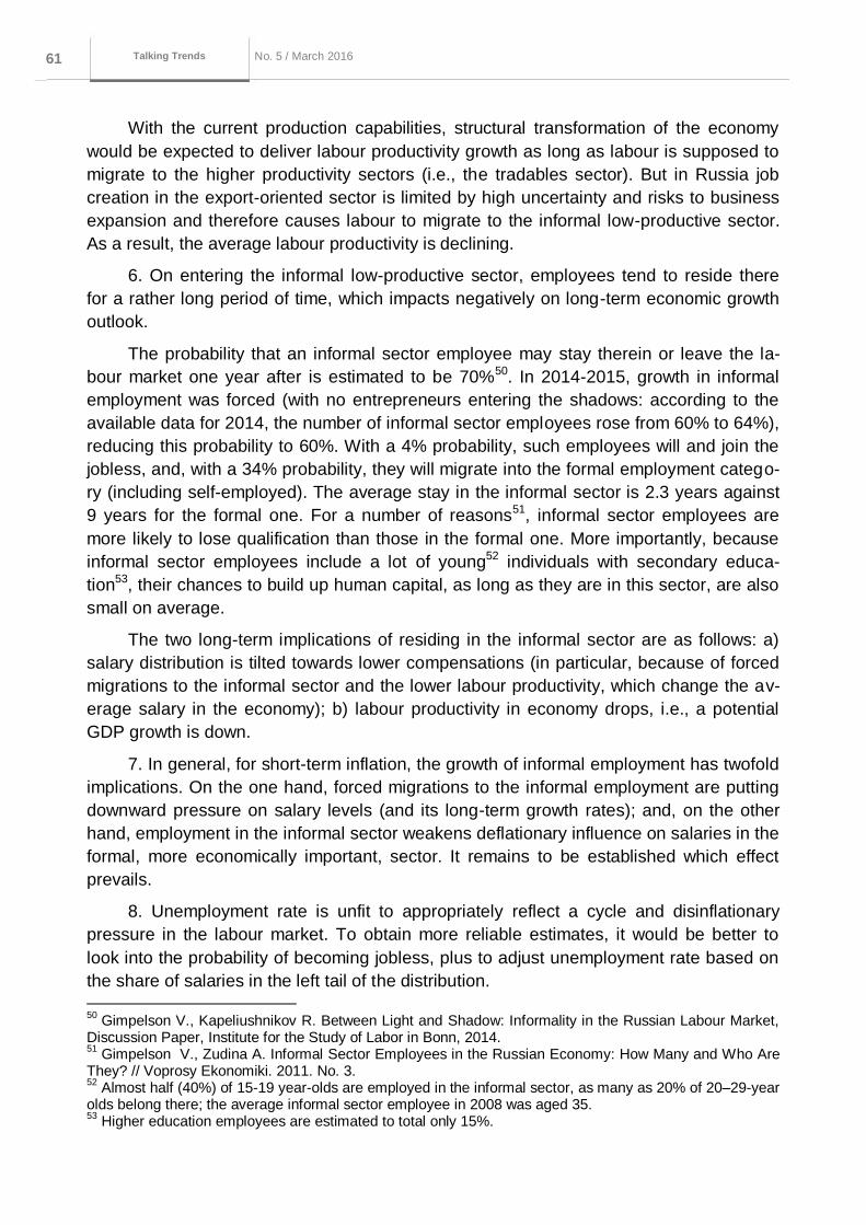
Серия до кла до в о б э ко но мичеСких
иССледо ва ниях 61 No. 5 / March 2016
Macroeconomics and markets No. 1 / October
2015
Talking Trends
With the current production capabilities, structural transformation of the economy
would be expected to deliver labour productivity growth as long as labour is supposed to
migrate to the higher productivity sectors (i.e., the tradables sector). But in Russia job
creation in the export-oriented sector is limited by high uncertainty and risks to business
expansion and therefore causes labour to migrate to the informal low-productive sector.
As a result, the average labour productivity is declining.
6. On entering the informal low-productive sector, employees tend to reside there
for a rather long period of time, which impacts negatively on long-term economic growth
outlook.
The probability that an informal sector employee may stay therein or leave the la-
bour market one year after is estimated to be 70%50. In 2014-2015, growth in informal
employment was forced (with no entrepreneurs entering the shadows: according to the
available data for 2014, the number of informal sector employees rose from 60% to 64%),
reducing this probability to 60%. With a 4% probability, such employees will and join the
jobless, and, with a 34% probability, they will migrate into the formal employment catego-
ry (including self-employed). The average stay in the informal sector is 2.3 years against
9 years for the formal one. For a number of reasons51, informal sector employees are
more likely to lose qualification than those in the formal one. More importantly, because
informal sector employees include a lot of young52 individuals with secondary educa-
tion53, their chances to build up human capital, as long as they are in this sector, are also
small on average.
The two long-term implications of residing in the informal sector are as follows: a)
salary distribution is tilted towards lower compensations (in particular, because of forced
migrations to the informal sector and the lower labour productivity, which change the av-
erage salary in the economy); b) labour productivity in economy drops, i.e., a potential
GDP growth is down.
7. In general, for short-term inflation, the growth of informal employment has twofold
implications. On the one hand, forced migrations to the informal employment are putting
downward pressure on salary levels (and its long-term growth rates); and, on the other
hand, employment in the informal sector weakens deflationary influence on salaries in the
formal, more economically important, sector. It remains to be established which effect
prevails.
8. Unemployment rate is unfit to appropriately reflect a cycle and disinflationary
pressure in the labour market. To obtain more reliable estimates, it would be better to
look into the probability of becoming jobless, plus to adjust unemployment rate based on
the share of salaries in the left tail of the distribution.
50
Gimpelson V., Kapeliushnikov R. Between Light and Shadow: Informality in the Russian Labour Market, Discussion Paper, Institute for the Study of Labor in Bonn, 2014. 51
Gimpelson V., Zudina A. Informal Sector Employees in the Russian Economy: How Many and Who Are They? // Voprosy Ekonomiki. 2011. No. 3. 52
Almost half (40%) of 15-19 year-olds are employed in the informal sector, as many as 20% of 20–29-year olds belong there; the average informal sector employee in 2008 was aged 35. 53
Higher education employees are estimated to total only 15%.
Серия до кла до в о б э ко но мичеСких
иССледо ва ниях 62 No. 5 / March 2016
Macroeconomics and markets No. 1 / October
2015
Talking Trends
9. Informal employment is an important obstacle for structural shifts in the economy.
It is necessary to drag down uncertainty as a production growth factor and to reduce in-
formal employment through this.
10. In the future as demand resumes to grow, it would have stronger inflation effect
because of higher informal employment.
The probability for a comeback from unemployment to the formal sector is higher
than that from the informal to formal sector (30% versus 25%). When demand growth re-
sumes, it will be of proinflationary nature as it is hard to come back from informal unem-
ployment. The growing sector is expected to call for more labour utilisation and then more
employment, though the latter may fail to oblige. It is important to look into salaries in the
tradables sector, which is a growth engine for the economy wherein the first signs of infla-
tion are likely to manifest themselves.

Серия до кла до в о б э ко но мичеСких
иССледо ва ниях 63 No. 5 / March 2016
Macroeconomics and markets No. 1 / October
2015
Talking Trends
Research and Forecasting Department
Alexander Morozov
Director
Sergey Vlasov
Elena Deryugina
Ekaterina Ilicheva
Natalia Karlova
Dmitry Kreptsev
Alexey Ponomarenko
Alexey Porshakov
Sergey Seleznev
Andrey Sinyakov
Dmitry Chernyadyev
Ksenia Yakovleva


![Consumer Trends in Russia regions for your business [ENG]](https://img.dokumen.tips/doc/110x75/55caad24bb61ebf20c8b4578/consumer-trends-in-russia-regions-for-your-business-eng.jpg)