tail bounds

tail bounds

For a random variable X, the tails of X are the parts of the PMF that are “far” from its mean.

2

binomial tails

3

heavy-tailed distribution

6

-3 -2 -1 0 1 2 3

0.0

0.1

0.2

0.3

0.4

X

density

heavy-tailed distribution

7

tail bounds

Often, we want to bound the probability that a random variable X is “large.” Perhaps:

9

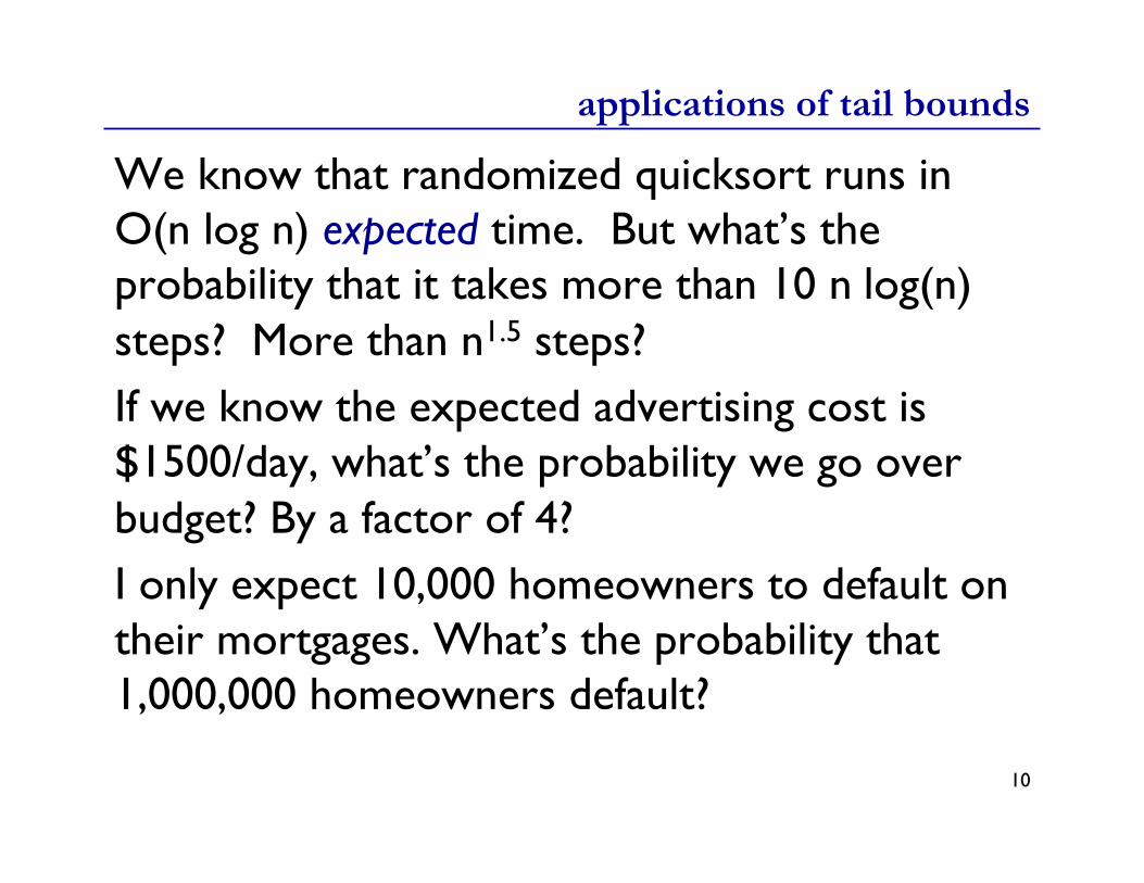
applications of tail bounds

We know that randomized quicksort runs in ���O(n log n) expected time. But what’s the probability that it takes more than 10 n log(n) steps? More than n1.5 steps? If we know the expected advertising cost is $1500/day, what’s the probability we go over budget? By a factor of 4? I only expect 10,000 homeowners to default on their mortgages. What’s the probability that 1,000,000 homeowners default?

10

the lake wobegon effect

“Lake Wobegon, Minnesota, where all the women are strong, ���

all the men are good looking, ���and ���

all the children are above average…”

11

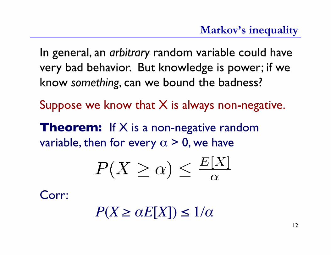
Markov’s inequality

In general, an arbitrary random variable could have very bad behavior. But knowledge is power; if we know something, can we bound the badness?

Suppose we know that X is always non-negative.

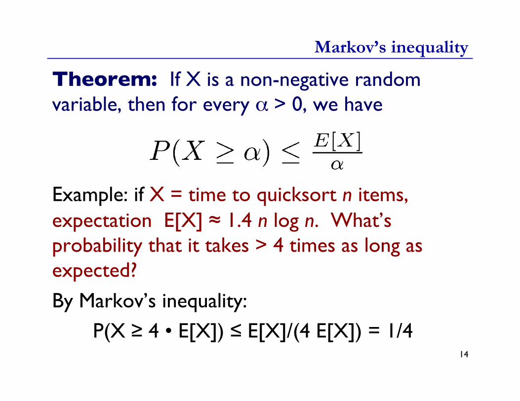
Theorem: If X is a non-negative random variable, then for every α > 0, we have

Corr: P(X ≥ αE[X]) ≤ 1/α

12

Markov’s inequality

Theorem: If X is a non-negative random variable, then for every α > 0, we have Example: if X = time to quicksort n items, expectation E[X] ≈ 1.4 n log n. What’s probability that it takes > 4 times as long as expected?

By Markov’s inequality: P(X ≥ 4 • E[X]) ≤ E[X]/(4 E[X]) = 1/4 14

Markov’s inequality

Theorem: If X is a non-negative random variable, then for every α > 0, we have

Proof:

E[X] = Σx xP(x)

= Σx<α xP(x) + Σx≥α xP(x)

≥ 0 + Σx≥ααP(x)

= αP(X ≥ α) 15

(x ≥ 0; α ≤ x)

Markov’s inequality

Theorem: If X is a non-negative random variable, then for every α > 0, we have

Proof:

E[X] = Σx xP(x)

= Σx<α xP(x) + Σx≥α xP(x)

≥ 0 + Σx≥ααP(x)

= αP(X ≥ α) 16

(x ≥ 0; α ≤ x)

Chebyshev’s inequality

If we know more about a random variable, we can often use that to get better tail bounds. Suppose we also know the variance.

Theorem: If Y is an arbitrary random variable with E[Y] = µ, then, for any α > 0,

17

Chebyshev’s inequality

Theorem: If Y is an arbitrary random variable with µ = E[Y], then, for any α > 0,

X is non-negative, so we can apply Markov’s inequality:

Proof:

18

Chebyshev’s inequality

Theorem: If Y is an arbitrary random variable with µ = E[Y], then, for any α > 0,

X is non-negative, so we can apply Markov’s inequality:

Proof:

19

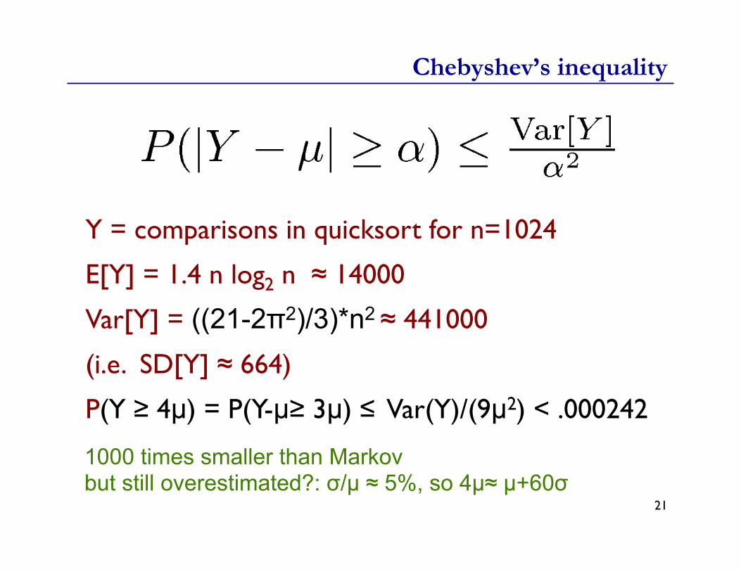
Chebyshev’s inequality

Y = comparisons in quicksort for n=1024

E[Y] = 1.4 n log2 n ≈ 14000

Var[Y] = ((21-2π2)/3)*n2 ≈ 441000

(i.e. SD[Y] ≈ 664)

P(Y ≥ 4µ) = P(Y-µ≥ 3µ) ≤ Var(Y)/(9µ2) < .000242

1000 times smaller than Markov but still overestimated?: σ/µ ≈ 5%, so 4µ≈ µ+60σ

21

Chebyshev’s inequality

Theorem: If Y is an arbitrary random variable with µ = E[Y], then, for any α > 0, Corr: If Then:

22

Chebyshev’s inequality

23

2

super strong tail bounds

Y ~ Bin(15000, 0.1) µ = E[Y] = 1500, σ = √Var(Y) = 36.7

P(Y ≥ 6000) = P(Y ≥ 4µ) ≤ ¼ (Markov) P(Y ≥ 6000) = P(Y-µ≥ 122σ) ≤ 7x10-5 (Chebyshev)

Poisson approximation: Y ~ Poi(1500) Rough computer calculation:

P(Y > 6000) << 10-1600

25

Chernoff bounds

Suppose X ~ Bin(n,p) µ = E[X] = pn Chernoff bound:

26

Chernoff bounds

Suppose X ~ Bin(n,p) µ = E[X] = pn

Chernoff bound:

27

router buffers

28

router buffers

Model: 100,000 computers each independently send a packet with probability p = 0.01 each second. The router processes its buffer every second. How many packet buffers so that router drops a packet: • Never? 100,000 • With probability at most 10-6, every hour? 1210 • With probability at most 10-6, every year? 1250 • With probability at most 10-6, since Big Bang? 1331

29

router buffers

X ~ Bin(100,000, 0.01), µ = E[X] = 1000 Let p = probability of buffer overflow in 1 second By the Chernoff bound Overflow probability in n seconds ��� = 1-(1-p)n ≤ np ≤ n exp(- δ2µ/2), which is ≤ ε provided δ ≥ √(2/µ)ln(n/ε). For ε=10-6 per hour: δ ≈ .210, buffers = 1210 For ε=10-6 per year: δ ≈ .250, buffers = 1250 For ε=10-6 per 15BY: δ ≈ .331, buffers = 1331

p =

31

summary

Tail bounds – bound probabilities of extreme events Three (of many): Markov: P(X ≥ kµ) ≤ 1/k (weak, but general; only need X ≥ 0 and µ)

Chebyshev: P(|X-µ| ≥ kσ) ≤ 1/k2 (often stronger, but also need σ)

Chernoff: various forms, depending on underlying distribution; usually 1/exponential, vs 1/polynomial above

Generally, more assumptions/knowledge ⇒ better bounds

“Better” than exact distribution? Maybe, e.g. if later is unknown or mathematically messy

“Better” than, e.g., “Poisson approx to Binomial”? Maybe, e.g. if you need rigorously “≤” rather than just “≈”

33