Embed Size (px)
Citation preview

Air Force Institute of TechnologyAFIT Scholar
Theses and Dissertations Student Graduate Works
3-26-2015
Tactical AI in Real Time Strategy GamesDonald A. Gruber
Follow this and additional works at: https://scholar.afit.edu/etd
Part of the Artificial Intelligence and Robotics Commons
This Thesis is brought to you for free and open access by the Student Graduate Works at AFIT Scholar. It has been accepted for inclusion in Theses andDissertations by an authorized administrator of AFIT Scholar. For more information, please contact [email protected].
Recommended CitationGruber, Donald A., "Tactical AI in Real Time Strategy Games" (2015). Theses and Dissertations. 30.https://scholar.afit.edu/etd/30

TACTICAL AI INREAL TIME STRATEGY GAMES
THESIS
Donald A. Gruber, Capt, USAF
AFIT-ENG-MS-15-M-021
DEPARTMENT OF THE AIR FORCEAIR UNIVERSITY
AIR FORCE INSTITUTE OF TECHNOLOGY
Wright-Patterson Air Force Base, Ohio
DISTRIBUTION STATEMENT AAPPROVED FOR PUBLIC RELEASE; DISTRIBUTION UNLIMITED.

The views expressed in this document are those of the author and do not reflect theofficial policy or position of the United States Air Force, the United States Departmentof Defense or the United States Government. This material is declared a work of theU.S. Government and is not subject to copyright protection in the United States.

AFIT-ENG-MS-15-M-021
TACTICAL AI IN
REAL TIME STRATEGY GAMES
THESIS
Presented to the Faculty
Department of Electrical Engineering
Graduate School of Engineering and Management
Air Force Institute of Technology
Air University
Air Education and Training Command
in Partial Fulfillment of the Requirements for the
Degree of Master of Science in Electrical Engineering
Donald A. Gruber, B.S.E.E.
Capt, USAF
March 2015
DISTRIBUTION STATEMENT AAPPROVED FOR PUBLIC RELEASE; DISTRIBUTION UNLIMITED.

AFIT-ENG-MS-15-M-021
TACTICAL AI IN
REAL TIME STRATEGY GAMES
THESIS
Donald A. Gruber, B.S.E.E.Capt, USAF
Committee Membership:
Dr. G. LamontChair
Dr. B. BorghettiMember
Maj B. Woolley, PhDMember

AFIT-ENG-MS-15-M-021
Abstract
The real time strategy (RTS) tactical decision making problem is a difficult problem.
It is generally more complex due to its high degree of time sensitivity. Not only must
a variety of unit maneuvers for each unit taking part in a battle be analyzed, the
decision must be made before the battlefield changes to the point that the decision is
no longer viable. This research effort presents a novel approach to this problem within
an educational, teaching objective. Particular decision focus is target selection for a
artificial intelligence (AI) RTS game model. The use of multi-objective evolutionary
algorithms (MOEAs) in this tactical decision making problem allows an AI agent
to make fast, effective solutions that do not require modification to fit the current
environment. This approach allows for the creation of a generic solution building
tool that is capable of performing well against scripted opponents without requiring
expert training or deep tree searches.
The RTS AI development occurs in three distinct phases. The first of which is
the integration of a MOEA software library into an existing open source RTS game
engine. This integration also includes the development of a new tactics decision
manager that is combined with the existing Air Force Institute of Technology AI
agent for RTS games. The next phase of research includes the testing and analysis of
various different MOEAs in order to determine which search method is most optimal
for the tactical decision making problem. The final phase of the research involves
analysis of the online performance of the newly developed tactics manager against a
variety of scripted agents. The experimental results validate that MOEAs can control
an on-line agent capable of out performing a variety AI RTS opponent test scripts.
iv

Acknowledgements
I would like to thank Dr. Gary Lamont for sharing his wealth of knowledge and
guiding me to new ideas and concepts that greatly assisted with this research effort.
I would also like to thank Jonathan Di Trapani and Jason Blackford for their insight
and advice.
Donald A. Gruber
v

Table of Contents
Page
Abstract . . . . . . . . . . . . . . . . . . . . . . . . . . . . . . . . . . . . . . . . . . . . . . . . . . . . . . . . . . . . . . . iv
Acknowledgements . . . . . . . . . . . . . . . . . . . . . . . . . . . . . . . . . . . . . . . . . . . . . . . . . . . . . . . v
List of Figures . . . . . . . . . . . . . . . . . . . . . . . . . . . . . . . . . . . . . . . . . . . . . . . . . . . . . . . . . . . x
List of Tables . . . . . . . . . . . . . . . . . . . . . . . . . . . . . . . . . . . . . . . . . . . . . . . . . . . . . . . . . . xiii
List of Acronyms . . . . . . . . . . . . . . . . . . . . . . . . . . . . . . . . . . . . . . . . . . . . . . . . . . . . . . xviii
I. Introduction . . . . . . . . . . . . . . . . . . . . . . . . . . . . . . . . . . . . . . . . . . . . . . . . . . . . . . . . 1
1.1 Military Decision Making . . . . . . . . . . . . . . . . . . . . . . . . . . . . . . . . . . . . . . . . . 11.2 Real Time Strategy Games . . . . . . . . . . . . . . . . . . . . . . . . . . . . . . . . . . . . . . . 2
Strategy in Real Time Strategy Games . . . . . . . . . . . . . . . . . . . . . . . . . . . . . 3Targeting in Real Time Strategy Games . . . . . . . . . . . . . . . . . . . . . . . . . . . . 4
1.3 Research Goal . . . . . . . . . . . . . . . . . . . . . . . . . . . . . . . . . . . . . . . . . . . . . . . . . . 41.4 Research Objectives . . . . . . . . . . . . . . . . . . . . . . . . . . . . . . . . . . . . . . . . . . . . . 51.5 Research Approach . . . . . . . . . . . . . . . . . . . . . . . . . . . . . . . . . . . . . . . . . . . . . . 51.6 Thesis Organization . . . . . . . . . . . . . . . . . . . . . . . . . . . . . . . . . . . . . . . . . . . . . 6
II. Background . . . . . . . . . . . . . . . . . . . . . . . . . . . . . . . . . . . . . . . . . . . . . . . . . . . . . . . . 7
2.1 Decision Making . . . . . . . . . . . . . . . . . . . . . . . . . . . . . . . . . . . . . . . . . . . . . . . . 7OODA Loop . . . . . . . . . . . . . . . . . . . . . . . . . . . . . . . . . . . . . . . . . . . . . . . . . . . . 8Thin Slicing . . . . . . . . . . . . . . . . . . . . . . . . . . . . . . . . . . . . . . . . . . . . . . . . . . . 10Making Decisions with Current State Analysis . . . . . . . . . . . . . . . . . . . . . . 10Research Goal . . . . . . . . . . . . . . . . . . . . . . . . . . . . . . . . . . . . . . . . . . . . . . . . . 11
2.2 Real Time Strategy (RTS) Games . . . . . . . . . . . . . . . . . . . . . . . . . . . . . . . . 12Dune II . . . . . . . . . . . . . . . . . . . . . . . . . . . . . . . . . . . . . . . . . . . . . . . . . . . . . . . 14WarCraft . . . . . . . . . . . . . . . . . . . . . . . . . . . . . . . . . . . . . . . . . . . . . . . . . . . . . . 14StarCraft . . . . . . . . . . . . . . . . . . . . . . . . . . . . . . . . . . . . . . . . . . . . . . . . . . . . . . 15Tactical Airpower Visualization . . . . . . . . . . . . . . . . . . . . . . . . . . . . . . . . . . 16Combining First Person Shooters with RTS Games . . . . . . . . . . . . . . . . . 18
2.3 RTS Platforms . . . . . . . . . . . . . . . . . . . . . . . . . . . . . . . . . . . . . . . . . . . . . . . . . 19Wargus . . . . . . . . . . . . . . . . . . . . . . . . . . . . . . . . . . . . . . . . . . . . . . . . . . . . . . . 19SparCraft . . . . . . . . . . . . . . . . . . . . . . . . . . . . . . . . . . . . . . . . . . . . . . . . . . . . . 19Spring Real Time Strategy (RTS) Engine . . . . . . . . . . . . . . . . . . . . . . . . . . 20
2.4 Strategic Decision Making . . . . . . . . . . . . . . . . . . . . . . . . . . . . . . . . . . . . . . . 212.5 Tactical Decision Making in Combat Scenarios . . . . . . . . . . . . . . . . . . . . . 232.6 Previous AFIT Developments . . . . . . . . . . . . . . . . . . . . . . . . . . . . . . . . . . . . 25
Adaptive Response - Weissgerber’s Agent . . . . . . . . . . . . . . . . . . . . . . . . . . 26Strategy Optimization - Di Trapani’s Agent . . . . . . . . . . . . . . . . . . . . . . . . 26
vi

Page
Build Order Optimization - Blackford’s Agent . . . . . . . . . . . . . . . . . . . . . . 27Tactics Optimization - AFIT Agent Continuing Work . . . . . . . . . . . . . . . 27
2.7 Current Research in RTS Tactics Optimization . . . . . . . . . . . . . . . . . . . . . 28Reinforcement Learning . . . . . . . . . . . . . . . . . . . . . . . . . . . . . . . . . . . . . . . . . 29Game-Tree Search . . . . . . . . . . . . . . . . . . . . . . . . . . . . . . . . . . . . . . . . . . . . . . 30Monte Carlo Planning . . . . . . . . . . . . . . . . . . . . . . . . . . . . . . . . . . . . . . . . . . 30Genetic Algorithms . . . . . . . . . . . . . . . . . . . . . . . . . . . . . . . . . . . . . . . . . . . . . 32Computational Agent Distribution . . . . . . . . . . . . . . . . . . . . . . . . . . . . . . . . 32
2.8 Multi-Objective Evolutionary Algorithm Tactics . . . . . . . . . . . . . . . . . . . . 342.9 Multi Objective Evolutionary Algorithms (MOEAs) . . . . . . . . . . . . . . . . . 34
Pareto Front Indicators . . . . . . . . . . . . . . . . . . . . . . . . . . . . . . . . . . . . . . . . . 39MOEA Software . . . . . . . . . . . . . . . . . . . . . . . . . . . . . . . . . . . . . . . . . . . . . . . . 41
2.10 Chapter Summary . . . . . . . . . . . . . . . . . . . . . . . . . . . . . . . . . . . . . . . . . . . . . . 43
III. Methodology of RTS Tactical Design . . . . . . . . . . . . . . . . . . . . . . . . . . . . . . . . . . 44
3.1 Introduction . . . . . . . . . . . . . . . . . . . . . . . . . . . . . . . . . . . . . . . . . . . . . . . . . . . 443.2 Overview of Research Approach . . . . . . . . . . . . . . . . . . . . . . . . . . . . . . . . . . 453.3 MOEA Software Selection . . . . . . . . . . . . . . . . . . . . . . . . . . . . . . . . . . . . . . . 463.4 Design Phase 1 - Integrating Spring RTS & PyGMO . . . . . . . . . . . . . . . 46
AFIT Agent . . . . . . . . . . . . . . . . . . . . . . . . . . . . . . . . . . . . . . . . . . . . . . . . . . . 48PyGMO . . . . . . . . . . . . . . . . . . . . . . . . . . . . . . . . . . . . . . . . . . . . . . . . . . . . . . 52Custom Tactics Optimization Problem . . . . . . . . . . . . . . . . . . . . . . . . . . . . 54Instantly Spawning Units in Spring . . . . . . . . . . . . . . . . . . . . . . . . . . . . . . . 54
3.5 Design Phase 2 - Developing Off-line Simulations . . . . . . . . . . . . . . . . . . . 55MOEAs Under Test . . . . . . . . . . . . . . . . . . . . . . . . . . . . . . . . . . . . . . . . . . . . 56Off-Line MOEA Objectives . . . . . . . . . . . . . . . . . . . . . . . . . . . . . . . . . . . . . . 57Objective Selected for Use in Offline Simulation . . . . . . . . . . . . . . . . . . . . 61Measuring MOEA Performance . . . . . . . . . . . . . . . . . . . . . . . . . . . . . . . . . . 62
3.6 Experimental Phase 3 - Developing On-Line Simulations . . . . . . . . . . . . . 62RTS Tactic Methods . . . . . . . . . . . . . . . . . . . . . . . . . . . . . . . . . . . . . . . . . . . . 62Measuring Battle Outcomes . . . . . . . . . . . . . . . . . . . . . . . . . . . . . . . . . . . . . . 69
3.7 Chapter Summary . . . . . . . . . . . . . . . . . . . . . . . . . . . . . . . . . . . . . . . . . . . . . . 71
IV. Design of Experiments . . . . . . . . . . . . . . . . . . . . . . . . . . . . . . . . . . . . . . . . . . . . . . 73
4.1 Introduction . . . . . . . . . . . . . . . . . . . . . . . . . . . . . . . . . . . . . . . . . . . . . . . . . . . 734.2 Experimental Design . . . . . . . . . . . . . . . . . . . . . . . . . . . . . . . . . . . . . . . . . . . . 734.3 Computer Platform and Software Layout . . . . . . . . . . . . . . . . . . . . . . . . . . 754.4 Design Phase 1 - Integration of Spring RTS and PyGMO . . . . . . . . . . . . 754.5 Design Phase 2 - Offline Simulation . . . . . . . . . . . . . . . . . . . . . . . . . . . . . . . 80
Testing MOEA Parameters . . . . . . . . . . . . . . . . . . . . . . . . . . . . . . . . . . . . . . 81Measurement Metrics . . . . . . . . . . . . . . . . . . . . . . . . . . . . . . . . . . . . . . . . . . . 81
4.6 Testing of Phase 3 - Online Simulation . . . . . . . . . . . . . . . . . . . . . . . . . . . . 85
vii

Page
Tactical Methods to be Tested . . . . . . . . . . . . . . . . . . . . . . . . . . . . . . . . . . . 86Online Simulation Measurement Metrics . . . . . . . . . . . . . . . . . . . . . . . . . . . 90
4.7 Chapter Summary . . . . . . . . . . . . . . . . . . . . . . . . . . . . . . . . . . . . . . . . . . . . . . 92
V. Results and Analysis . . . . . . . . . . . . . . . . . . . . . . . . . . . . . . . . . . . . . . . . . . . . . . . . 93
5.1 Introduction . . . . . . . . . . . . . . . . . . . . . . . . . . . . . . . . . . . . . . . . . . . . . . . . . . . 935.2 Design Phase 1 - Integrating Spring and PyGMO . . . . . . . . . . . . . . . . . . . 935.3 Testing of Phase 2 - Offline Simulation . . . . . . . . . . . . . . . . . . . . . . . . . . . . 97
Analysis of MOEA Performance in Tactics Optimization . . . . . . . . . . . . . 97Conclusions of Offline Simulation . . . . . . . . . . . . . . . . . . . . . . . . . . . . . . . . 105
5.4 Phase 3 - Online Simulation . . . . . . . . . . . . . . . . . . . . . . . . . . . . . . . . . . . . 106Analysis of the Default Tactic . . . . . . . . . . . . . . . . . . . . . . . . . . . . . . . . . . . 107Analysis of the Proximity Tactic . . . . . . . . . . . . . . . . . . . . . . . . . . . . . . . . . 107Analysis of the Weak Tactic . . . . . . . . . . . . . . . . . . . . . . . . . . . . . . . . . . . . 108Analysis of the MOEA Tactic . . . . . . . . . . . . . . . . . . . . . . . . . . . . . . . . . . . 109Comparison of Tactical Results . . . . . . . . . . . . . . . . . . . . . . . . . . . . . . . . . . 109Conclusions of On-Line Battles . . . . . . . . . . . . . . . . . . . . . . . . . . . . . . . . . . 116
5.5 Comparison of Results to Previous Research . . . . . . . . . . . . . . . . . . . . . . 1165.6 Chapter Summary . . . . . . . . . . . . . . . . . . . . . . . . . . . . . . . . . . . . . . . . . . . . . 117
VI. Conclusion . . . . . . . . . . . . . . . . . . . . . . . . . . . . . . . . . . . . . . . . . . . . . . . . . . . . . . . 119
6.1 Evaluation of Results . . . . . . . . . . . . . . . . . . . . . . . . . . . . . . . . . . . . . . . . . . 1196.2 Future Work . . . . . . . . . . . . . . . . . . . . . . . . . . . . . . . . . . . . . . . . . . . . . . . . . . 1216.3 Final Remarks . . . . . . . . . . . . . . . . . . . . . . . . . . . . . . . . . . . . . . . . . . . . . . . . 122
Appendix A. Code for Offline Simulation . . . . . . . . . . . . . . . . . . . . . . . . . . . . . . . . . 123
1.1 moea.py . . . . . . . . . . . . . . . . . . . . . . . . . . . . . . . . . . . . . . . . . . . . . . . . . . . . . . 1231.2 group.py . . . . . . . . . . . . . . . . . . . . . . . . . . . . . . . . . . . . . . . . . . . . . . . . . . . . . 1261.3 agent.py . . . . . . . . . . . . . . . . . . . . . . . . . . . . . . . . . . . . . . . . . . . . . . . . . . . . . 1401.4 config.txt . . . . . . . . . . . . . . . . . . . . . . . . . . . . . . . . . . . . . . . . . . . . . . . . . . . . . 143
Appendix B. Raw Data for Offline Simulation . . . . . . . . . . . . . . . . . . . . . . . . . . . . . 144
2.1 Data for NSGA-II Algorithm. . . . . . . . . . . . . . . . . . . . . . . . . . . . . . . . . . . . 144NSGA-II Algorithm Data for 20 Population . . . . . . . . . . . . . . . . . . . . . . . 144NSGA-II Algorithm Data for 40 Population . . . . . . . . . . . . . . . . . . . . . . . 147NSGA-II Algorithm Data for 60 Population . . . . . . . . . . . . . . . . . . . . . . . 149NSGA-II Algorithm Data for 80 Population . . . . . . . . . . . . . . . . . . . . . . . 151NSGA-II Algorithm Data for 80 Population . . . . . . . . . . . . . . . . . . . . . . . 153
2.2 Data for SPEA2 Algorithm . . . . . . . . . . . . . . . . . . . . . . . . . . . . . . . . . . . . . 155SPEA2 Algorithm Data for 20 Population . . . . . . . . . . . . . . . . . . . . . . . . 155SPEA2 Algorithm Data for 40 Population . . . . . . . . . . . . . . . . . . . . . . . . 157SPEA2 Algorithm Data for 60 Population . . . . . . . . . . . . . . . . . . . . . . . . 159
viii

Page
SPEA2 Algorithm Data for 80 Population . . . . . . . . . . . . . . . . . . . . . . . . 161SPEA2 Algorithm Data for 80 Population . . . . . . . . . . . . . . . . . . . . . . . . 163
2.3 Data for NSPSO Algorithm . . . . . . . . . . . . . . . . . . . . . . . . . . . . . . . . . . . . . 165NSPSO Algorithm Data for 20 Population . . . . . . . . . . . . . . . . . . . . . . . . 165NSPSO Algorithm Data for 40 Population . . . . . . . . . . . . . . . . . . . . . . . . 167NSPSO Algorithm Data for 60 Population . . . . . . . . . . . . . . . . . . . . . . . . 169NSPSO Algorithm Data for 80 Population . . . . . . . . . . . . . . . . . . . . . . . . 171NSPSO Algorithm Data for 100 Population . . . . . . . . . . . . . . . . . . . . . . . 173
Appendix C. Raw Data for Online Simulation . . . . . . . . . . . . . . . . . . . . . . . . . . . . . 175
3.1 Data for MOEA Tactic Starting From Top of Map . . . . . . . . . . . . . . . . . 1753.2 Data for Default Tactic Starting From Top of Map . . . . . . . . . . . . . . . . . 1773.3 Data for Proximity Tactic Starting from Top of Map . . . . . . . . . . . . . . . 1793.4 Data for Weak Tactic Starting from Top of Map . . . . . . . . . . . . . . . . . . . 181
Appendix D. Online Simulation Data Sorted by Winner . . . . . . . . . . . . . . . . . . . . 183
4.1 MOEA Tactic Victory Statistics . . . . . . . . . . . . . . . . . . . . . . . . . . . . . . . . . 1834.2 Default Tactic Victory Statistics . . . . . . . . . . . . . . . . . . . . . . . . . . . . . . . . . 1864.3 Proximity Tactic Victory Statistics . . . . . . . . . . . . . . . . . . . . . . . . . . . . . . 1884.4 Weak Tactic Victory Statistics . . . . . . . . . . . . . . . . . . . . . . . . . . . . . . . . . . 190
Bibliography . . . . . . . . . . . . . . . . . . . . . . . . . . . . . . . . . . . . . . . . . . . . . . . . . . . . . . . . . . 191
ix

List of Figures
Figure Page
1 Boyd’s OODA Loop [1] . . . . . . . . . . . . . . . . . . . . . . . . . . . . . . . . . . . . . . . . . . . 8
2 Screenshot of Cosmic Conquest [2] . . . . . . . . . . . . . . . . . . . . . . . . . . . . . . . . 13
3 Screenshot of Dune II [3] . . . . . . . . . . . . . . . . . . . . . . . . . . . . . . . . . . . . . . . . 14
4 Screenshot of Warcraft [4] . . . . . . . . . . . . . . . . . . . . . . . . . . . . . . . . . . . . . . . . 15
5 RTS Strategic Planning Tree [5] . . . . . . . . . . . . . . . . . . . . . . . . . . . . . . . . . . 22
6 RTS Tactical Planning Tree . . . . . . . . . . . . . . . . . . . . . . . . . . . . . . . . . . . . . . 24
7 Example Pareto Front with Different Population Sizes(5, 10, 20, 50) . . . . . . . . . . . . . . . . . . . . . . . . . . . . . . . . . . . . . . . . . . . . . . . . . . 34
8 File layout for the Di Trapani (AFIT) Agent [6] . . . . . . . . . . . . . . . . . . . . . 47
9 File connection structure for the Di Trapani (AFIT)Agent [6] . . . . . . . . . . . . . . . . . . . . . . . . . . . . . . . . . . . . . . . . . . . . . . . . . . . . . . 50
10 Example for config.txt . . . . . . . . . . . . . . . . . . . . . . . . . . . . . . . . . . . . . . . . . . . 51
12 Example Solution for 3 vs 2 Combat . . . . . . . . . . . . . . . . . . . . . . . . . . . . . . 55
13 Code Representing Focus Fire Objective . . . . . . . . . . . . . . . . . . . . . . . . . . . 59
14 Pseudocode for Default AFIT Agent Tactics (GroupAttack Closest) . . . . . . . . . . . . . . . . . . . . . . . . . . . . . . . . . . . . . . . . . . . . . . . . . 64
15 Pseudocode for Individual Attack Closest . . . . . . . . . . . . . . . . . . . . . . . . . . 66
16 Pseudocode for Group Attack Weakest . . . . . . . . . . . . . . . . . . . . . . . . . . . . 67
17 Implementation of MOEA in AFIT Agent . . . . . . . . . . . . . . . . . . . . . . . . . . 68
18 Stumpy Tank . . . . . . . . . . . . . . . . . . . . . . . . . . . . . . . . . . . . . . . . . . . . . . . . . . 69
19 Central Path of ThePass map on Spring RTS Engine . . . . . . . . . . . . . . . . 70
20 Custom PyGMO Problem Created for TacticOptimization (Initialization) . . . . . . . . . . . . . . . . . . . . . . . . . . . . . . . . . . . . . 76
21 Custom PyGMO Problem Created for TacticOptimization (Calculation) . . . . . . . . . . . . . . . . . . . . . . . . . . . . . . . . . . . . . . . 78
x

Figure Page
22 Custom PyGMO Problem Created for TacticOptimization (Objectives) . . . . . . . . . . . . . . . . . . . . . . . . . . . . . . . . . . . . . . . 79
23 Starting Positions for Online Simulations . . . . . . . . . . . . . . . . . . . . . . . . . . 86
24 Default Tactic in Use . . . . . . . . . . . . . . . . . . . . . . . . . . . . . . . . . . . . . . . . . . . . 87
25 Proximity Tactic in Use . . . . . . . . . . . . . . . . . . . . . . . . . . . . . . . . . . . . . . . . . 88
26 Weak Tactic in Use . . . . . . . . . . . . . . . . . . . . . . . . . . . . . . . . . . . . . . . . . . . . . 89
27 MOEA Tactic in Use . . . . . . . . . . . . . . . . . . . . . . . . . . . . . . . . . . . . . . . . . . . . 90
28 Simulation of 25 Tanks Attacking a Single Point . . . . . . . . . . . . . . . . . . . . 94
29 Two Examples of 25 vs 25 Tank Battles . . . . . . . . . . . . . . . . . . . . . . . . . . . 94
30 Code Layout of the Initial Round of Combat . . . . . . . . . . . . . . . . . . . . . . . 95
31 Box Plots for HV Increase Over Time for NSGA-II 20Population . . . . . . . . . . . . . . . . . . . . . . . . . . . . . . . . . . . . . . . . . . . . . . . . . . . . . 99
32 Box Plots Showing HV Increase Over Time for NSGA-IIAlgorithm . . . . . . . . . . . . . . . . . . . . . . . . . . . . . . . . . . . . . . . . . . . . . . . . . . . . 100
33 Box Plots for HV Increase Over Time for SPEA2 20Population . . . . . . . . . . . . . . . . . . . . . . . . . . . . . . . . . . . . . . . . . . . . . . . . . . . . 101
34 Box Plots Showing HV Increase Over Time for SPEA2Algorithm . . . . . . . . . . . . . . . . . . . . . . . . . . . . . . . . . . . . . . . . . . . . . . . . . . . . 102
35 Box Plots for HV Increase Over Time for NSPSO 20Population . . . . . . . . . . . . . . . . . . . . . . . . . . . . . . . . . . . . . . . . . . . . . . . . . . . . 103
36 Box Plots Showing HV Increase Over Time for NSPSOAlgorithm . . . . . . . . . . . . . . . . . . . . . . . . . . . . . . . . . . . . . . . . . . . . . . . . . . . . 104
37 Comparison of Win Percentages Between Tactic Options . . . . . . . . . . . . 110
38 Comparison of Battle Duration Between Tactic Options . . . . . . . . . . . . . 111
39 Box Plots For Online Battle Duration . . . . . . . . . . . . . . . . . . . . . . . . . . . . 112
40 Comparison of Units Remaining After Battle BetweenTactic Options . . . . . . . . . . . . . . . . . . . . . . . . . . . . . . . . . . . . . . . . . . . . . . . . 112
xi

Figure Page
41 Box Plots For Number of Units Remaining . . . . . . . . . . . . . . . . . . . . . . . . 113
42 Comparison of Average Remaining HP After BattleBetween Tactic Options . . . . . . . . . . . . . . . . . . . . . . . . . . . . . . . . . . . . . . . . 114
43 Box Plots For Average HP Remaining . . . . . . . . . . . . . . . . . . . . . . . . . . . . 115
xii

List of Tables
Table Page
1 Layout of a Strategy in strategyDefs.txt . . . . . . . . . . . . . . . . . . . . . . . . . . . 51
2 HV Gain per Second for NSGA-II . . . . . . . . . . . . . . . . . . . . . . . . . . . . . . . . . 98
3 HV Gain per Second for SPEA2 . . . . . . . . . . . . . . . . . . . . . . . . . . . . . . . . . 100
4 HV Gain per Second for NSPSO . . . . . . . . . . . . . . . . . . . . . . . . . . . . . . . . . 102
5 Results of Default Tactic VS Other Tactics . . . . . . . . . . . . . . . . . . . . . . . . 107
6 Results of Proximity Tactic VS Other Tactics . . . . . . . . . . . . . . . . . . . . . 108
7 Results of Weak Tactic VS Other Tactics . . . . . . . . . . . . . . . . . . . . . . . . . 108
8 Results of MOEA Tactic VS Other Tactics . . . . . . . . . . . . . . . . . . . . . . . . 109
9 NSGA-II 20 Population, 2 Generations . . . . . . . . . . . . . . . . . . . . . . . . . . . 144
10 NSGA-II 20 Population, 3 Generations . . . . . . . . . . . . . . . . . . . . . . . . . . . 145
11 NSGA-II 20 Population, 4 Generations . . . . . . . . . . . . . . . . . . . . . . . . . . . 145
12 NSGA-II 20 Population, 5 Generations . . . . . . . . . . . . . . . . . . . . . . . . . . . 146
13 NSGA-II 40 Population, 2 Generations . . . . . . . . . . . . . . . . . . . . . . . . . . . 147
14 NSGA-II 40 Population, 3 Generations . . . . . . . . . . . . . . . . . . . . . . . . . . . 147
15 NSGA-II 40 Population, 4 Generations . . . . . . . . . . . . . . . . . . . . . . . . . . . 148
16 NSGA-II 40 Population, 5 Generations . . . . . . . . . . . . . . . . . . . . . . . . . . . 148
17 NSGA-II 60 Population, 2 Generations . . . . . . . . . . . . . . . . . . . . . . . . . . . 149
18 NSGA-II 60 Population, 3 Generations . . . . . . . . . . . . . . . . . . . . . . . . . . . 149
19 NSGA-II 60 Population, 4 Generations . . . . . . . . . . . . . . . . . . . . . . . . . . . 150
20 NSGA-II 60 Population, 5 Generations . . . . . . . . . . . . . . . . . . . . . . . . . . . 150
21 NSGA-II 80 Population, 2 Generations . . . . . . . . . . . . . . . . . . . . . . . . . . . 151
22 NSGA-II 80 Population, 3 Generations . . . . . . . . . . . . . . . . . . . . . . . . . . . 151
xiii

Table Page
23 NSGA-II 80 Population, 4 Generations . . . . . . . . . . . . . . . . . . . . . . . . . . . 152
24 NSGA-II 80 Population, 5 Generations . . . . . . . . . . . . . . . . . . . . . . . . . . . 152
25 NSGA-II 100 Population, 2 Generations . . . . . . . . . . . . . . . . . . . . . . . . . . 153
26 NSGA-II 100 Population, 3 Generations . . . . . . . . . . . . . . . . . . . . . . . . . . 153
27 NSGA-II 100 Population, 4 Generations . . . . . . . . . . . . . . . . . . . . . . . . . . 154
28 NSGA-II 100 Population, 5 Generations . . . . . . . . . . . . . . . . . . . . . . . . . . 154
29 SPEA2 20 Population, 2 Generations . . . . . . . . . . . . . . . . . . . . . . . . . . . . . 155
30 SPEA2 20 Population, 3 Generations . . . . . . . . . . . . . . . . . . . . . . . . . . . . . 155
31 SPEA2 20 Population, 4 Generations . . . . . . . . . . . . . . . . . . . . . . . . . . . . . 156
32 SPEA2 20 Population, 5 Generations . . . . . . . . . . . . . . . . . . . . . . . . . . . . . 156
33 SPEA2 40 Population, 2 Generations . . . . . . . . . . . . . . . . . . . . . . . . . . . . . 157
34 SPEA2 40 Population, 3 Generations . . . . . . . . . . . . . . . . . . . . . . . . . . . . . 157
35 SPEA2 40 Population, 4 Generations . . . . . . . . . . . . . . . . . . . . . . . . . . . . . 158
36 SPEA2 40 Population, 5 Generations . . . . . . . . . . . . . . . . . . . . . . . . . . . . . 158
37 SPEA2 60 Population, 2 Generations . . . . . . . . . . . . . . . . . . . . . . . . . . . . . 159
38 SPEA2 60 Population, 3 Generations . . . . . . . . . . . . . . . . . . . . . . . . . . . . . 159
39 SPEA2 60 Population, 4 Generations . . . . . . . . . . . . . . . . . . . . . . . . . . . . . 160
40 SPEA2 60 Population, 5 Generations . . . . . . . . . . . . . . . . . . . . . . . . . . . . . 160
41 SPEA2 80 Population, 2 Generations . . . . . . . . . . . . . . . . . . . . . . . . . . . . . 161
42 SPEA2 80 Population, 3 Generations . . . . . . . . . . . . . . . . . . . . . . . . . . . . . 161
43 SPEA2 80 Population, 4 Generations . . . . . . . . . . . . . . . . . . . . . . . . . . . . . 162
44 SPEA2 80 Population, 5 Generations . . . . . . . . . . . . . . . . . . . . . . . . . . . . . 162
45 SPEA2 100 Population, 2 Generations . . . . . . . . . . . . . . . . . . . . . . . . . . . . 163
46 SPEA2 100 Population, 3 Generations . . . . . . . . . . . . . . . . . . . . . . . . . . . . 163
xiv

Table Page
47 SPEA2 100 Population, 4 Generations . . . . . . . . . . . . . . . . . . . . . . . . . . . . 164
48 SPEA2 100 Population, 5 Generations . . . . . . . . . . . . . . . . . . . . . . . . . . . . 164
49 NSPSO 20 Population, 2 Generations . . . . . . . . . . . . . . . . . . . . . . . . . . . . . 165
50 NSPSO 20 Population, 3 Generations . . . . . . . . . . . . . . . . . . . . . . . . . . . . . 165
51 NSPSO 20 Population, 4 Generations . . . . . . . . . . . . . . . . . . . . . . . . . . . . . 166
52 NSPSO 20 Population, 5 Generations . . . . . . . . . . . . . . . . . . . . . . . . . . . . . 166
53 NSPSO 40 Population, 2 Generations . . . . . . . . . . . . . . . . . . . . . . . . . . . . . 167
54 NSPSO 40 Population, 3 Generations . . . . . . . . . . . . . . . . . . . . . . . . . . . . . 167
55 NSPSO 40 Population, 4 Generations . . . . . . . . . . . . . . . . . . . . . . . . . . . . . 168
56 NSPSO 40 Population, 5 Generations . . . . . . . . . . . . . . . . . . . . . . . . . . . . . 168
57 NSPSO 60 Population, 2 Generations . . . . . . . . . . . . . . . . . . . . . . . . . . . . . 169
58 NSPSO 60 Population, 3 Generations . . . . . . . . . . . . . . . . . . . . . . . . . . . . . 169
59 NSPSO 60 Population, 4 Generations . . . . . . . . . . . . . . . . . . . . . . . . . . . . . 170
60 NSPSO 60 Population, 5 Generations . . . . . . . . . . . . . . . . . . . . . . . . . . . . . 170
61 NSPSO 80 Population, 2 Generations . . . . . . . . . . . . . . . . . . . . . . . . . . . . . 171
62 NSPSO 80 Population, 3 Generations . . . . . . . . . . . . . . . . . . . . . . . . . . . . . 171
63 NSPSO 80 Population, 4 Generations . . . . . . . . . . . . . . . . . . . . . . . . . . . . . 172
64 NSPSO 80 Population, 5 Generations . . . . . . . . . . . . . . . . . . . . . . . . . . . . . 172
65 NSPSO 100 Population, 2 Generations . . . . . . . . . . . . . . . . . . . . . . . . . . . . 173
66 NSPSO 100 Population, 3 Generations . . . . . . . . . . . . . . . . . . . . . . . . . . . . 173
67 NSPSO 100 Population, 4 Generations . . . . . . . . . . . . . . . . . . . . . . . . . . . . 174
68 NSPSO 100 Population, 5 Generations . . . . . . . . . . . . . . . . . . . . . . . . . . . . 174
69 Online Simulation Results for MOEA Tactic vs DefaultTactic . . . . . . . . . . . . . . . . . . . . . . . . . . . . . . . . . . . . . . . . . . . . . . . . . . . . . . . . 175
xv

Table Page
70 Online Simulation Results for MOEA Tactic vsProximity Tactic . . . . . . . . . . . . . . . . . . . . . . . . . . . . . . . . . . . . . . . . . . . . . . 176
71 Online Simulation Results for MOEA Tactic vs WeakTactic . . . . . . . . . . . . . . . . . . . . . . . . . . . . . . . . . . . . . . . . . . . . . . . . . . . . . . . . 176
72 Online Simulation Results for Default Tactic vs MOEATactic . . . . . . . . . . . . . . . . . . . . . . . . . . . . . . . . . . . . . . . . . . . . . . . . . . . . . . . . 177
73 Online Simulation Results for Default Tactic vsProximity Tactic . . . . . . . . . . . . . . . . . . . . . . . . . . . . . . . . . . . . . . . . . . . . . . 178
74 Online Simulation Results for Default Tactic vs WeakTactic . . . . . . . . . . . . . . . . . . . . . . . . . . . . . . . . . . . . . . . . . . . . . . . . . . . . . . . . 178
75 Online Simulation Results for Proximity Tactic vsDefault Tactic . . . . . . . . . . . . . . . . . . . . . . . . . . . . . . . . . . . . . . . . . . . . . . . . . 179
76 Online Simulation Results for Proximity Tactic vsMOEA Tactic . . . . . . . . . . . . . . . . . . . . . . . . . . . . . . . . . . . . . . . . . . . . . . . . . 180
77 Online Simulation Results for Proximity Tactic vs WeakTactic . . . . . . . . . . . . . . . . . . . . . . . . . . . . . . . . . . . . . . . . . . . . . . . . . . . . . . . . 180
78 Online Simulation Results for Weak Tactic vs DefaultTactic . . . . . . . . . . . . . . . . . . . . . . . . . . . . . . . . . . . . . . . . . . . . . . . . . . . . . . . . 181
79 Online Simulation Results for Weak Tactic vs ProximityTactic . . . . . . . . . . . . . . . . . . . . . . . . . . . . . . . . . . . . . . . . . . . . . . . . . . . . . . . . 182
80 Online Simulation Results for Weak Tactic vs MOEATactic . . . . . . . . . . . . . . . . . . . . . . . . . . . . . . . . . . . . . . . . . . . . . . . . . . . . . . . . 182
81 Statistics for MOEA Tactic Victory against DefaultTactic . . . . . . . . . . . . . . . . . . . . . . . . . . . . . . . . . . . . . . . . . . . . . . . . . . . . . . . . 183
82 Statistics for MOEA Tactic Victory against ProximityTactic . . . . . . . . . . . . . . . . . . . . . . . . . . . . . . . . . . . . . . . . . . . . . . . . . . . . . . . . 184
83 Statistics for MOEA Tactic Victory against Weak Tactic . . . . . . . . . . . . 185
84 Statistics for Default Tactic Victory against MOEATactic . . . . . . . . . . . . . . . . . . . . . . . . . . . . . . . . . . . . . . . . . . . . . . . . . . . . . . . . 186
85 Statistics for Default Tactic Victory against ProximityTactic . . . . . . . . . . . . . . . . . . . . . . . . . . . . . . . . . . . . . . . . . . . . . . . . . . . . . . . . 186
xvi

Table Page
86 Statistics for Default Tactic Victory against Weak Tactic . . . . . . . . . . . . 187
87 Statistics for Proximity Tactic Victory against MOEATactic . . . . . . . . . . . . . . . . . . . . . . . . . . . . . . . . . . . . . . . . . . . . . . . . . . . . . . . . 188
88 Statistics for Proximity Tactic Victory against DefaultTactic . . . . . . . . . . . . . . . . . . . . . . . . . . . . . . . . . . . . . . . . . . . . . . . . . . . . . . . . 188
89 Statistics for Proximity Tactic Victory against WeakTactic . . . . . . . . . . . . . . . . . . . . . . . . . . . . . . . . . . . . . . . . . . . . . . . . . . . . . . . . 189
90 Statistics for Weak Tactic Victory against MOEA Tactic . . . . . . . . . . . . 190
91 Statistics for Weak Tactic Victory against Default Tactic . . . . . . . . . . . . 190
92 Statistics for Weak Tactic Victory against ProximityTactic . . . . . . . . . . . . . . . . . . . . . . . . . . . . . . . . . . . . . . . . . . . . . . . . . . . . . . . . 190
xvii

. List of Acronyms
AETC Air Education and Training Command
AFIT The Air Force Institute of Technology
AI Artificial Intelligence
BA Balanced Annihilation
ESA European Space Agency
FPS First Person Shooter
HA Hyperarea
HP Hit Points
HV hypervolume
GD Generational Distance
MCTS Monte Carlo Tree Search
MOEA Multi-Objective Evolutionary Algorithm
MOEAs Multi-Objective Evolutionary Algorithms
NFL No Free Lunch
NSGA Nondominated Sorting Genetic Algorithm
NSGA-II Nondominated Sorting Genetic Algorithm II
NSPSO Nondominated Sorting Particle Swarm Optimization
PSO Particle Swarm Optimization
xviii

RTS Real Time Strategy
SPEA Strength Pareto Evolutionary Algorithm
SPEA2 Strength Pareto Evolutionary Algorithm 2
TAV Tactical Airpower Visualization
xix

TACTICAL AI IN
REAL TIME STRATEGY GAMES
I. Introduction
This research aims to improve on current RTS Artificial Intelligence (AI) method-
ologies by introducing the concept of utilizing Multi-Objective Evolutionary Algo-
rithms (MOEAs) to quickly determine tactical actions to take in combat without
relying on search trees or expert data [7]. RTS games, along with video games in
general, provide an attractive means to test out these new AI techniques due to
their broad range of environments and lack of costs that real-world experimentation
requires [8]. The current state of an RTS game is also constantly changing, which
introduces a level of time-sensitivity which increases the necessity for quick decision
making.
1.1 Military Decision Making
The US Military holds the education of its forces as one of its major responsibili-
ties. The Air Force has an entire Major Command dedicated solely to this purpose,
Air Education and Training Command (AETC) [9]. One of the roles of AETC is
the training and development of officers with regard to strategic and tactical deci-
sion making. This decision making training is provided through many means, one of
which is to have officers perform various command level roles in a custom built RTS,
Tactical Airpower Visualization (TAV) [10]. Officers are taught many problem solv-
ing approaches prior to the exercise with TAV. One of the most important of these
processes is the OODA loop. OODA stands for Observe, Orient, Decide, and Act,
1

and was originally developed by John Boyd as a process to aid in decision making
[1]. The OODA loop is a four step decision making process which places emphasis
on a linear decision making pattern that can be used in many situations. First, the
user must Observe, or gather data pertaining to the problem at hand. Then the user
must Orient, or determine the potential effects from various decisions that could be
made for the problem. Then the best one of these potential solutions is Decided
and Acted upon. Once performed the user must go back and examine whether the
intended effects took place and if the problem is resolved. The research performed in
this thesis investigation replicates this four step process by utilizing MOEAs to make
a decision based on immediately available data and with no prior knowledge of the
opponents play style or decision making capacity.
1.2 Real Time Strategy Games
RTS games are a genre of video game which “are essentially simplified military
simulations [11].” In an RTS game, a player is responsible for developing an economic
supply life for his army via natural resources or other means, and then exploiting
these resources to produce and maintain a sizable military. The player then uses
this military to seek out and destroy enemy players. Each player’s approach to the
battle can be different, but the end state is based heavily on the strategic and tactical
decisions the player makes throughout the campaign.
The decision making required in an RTS game is very complex, as the game state
is constantly in flux. There are many segments of decision making in an RTS game as
well, which can all significantly affect the player’s capacity to win. Initially the player
must split effort between economic development and military development. A poor
decision at the start can significantly handicap a player’s future efforts by affecting
how many resources and units are available to repel enemy attacks. Even with a
2

proper base set up the player must still control individual units in battle. There
are AE potential attack combinations, with A representing the number of units in
the player’s army and E representing the number of enemy units. This is further
compounded by different unit armor, attack power, and ranges. A good RTS player
or agent must be able to make sound decisions in each of these environments in order
to win.
Strategy in Real Time Strategy Games.
Strategic decision making in RTS games are typically modified by changing the
focus of development between military, defense, or economy. Each strategy requires
that the player or agent hit various tech levels. Higher tech levels in RTS games allow
for the development of more powerful units. For example, a player at tech level 1
may have access to basic infantry units. Tech level 2 may allow for light vehicles and
rocket lauchers, and tech level 3 may allow the player to begin constructing tanks.
Players and agents enact different strategies by pursuing the requisite tech level for
their strategy, and then begin creating armies [12]. AI agents also have the benefit of
being able to “cheat”, or gather economic more quickly than what a human player is
capable of. This modification of resource acquisition capacity allows for an AI agent
to counter the human’s ability to learn and predict a particular agent’s strategy. By
improving resource acquisition the agent is more likely to overwhelm a human player
before effective countermeasures can be created.
The selection of a good strategy heavily affects the chance of victory between
players. Many strategies have distinct counters, and modifying one’s chosen strategy
to counter the opponent’s gives the player a distinct advantage in the long term per-
formance of the game [6]. The rate that a player is capable of building up a base
and army also affects the overall outcome of the match. If a player is able to outpro-
3

duce the opponent the player has a higher chance of winning as a higher production
leads to larger, more powerful armies. This production is based on the build order
of buildings and units, which, if optimized, can create noticeable improvements over
base strategies [5].
Targeting in Real Time Strategy Games.
There are many methods currently used for tactical decision making in RTS games,
otherwise known as “micro” for micromanagement of individual units and forces in
combat. Some of the fastest decision making tools are scripted attack methods. In
a scripted tactic the agent looks for a particular element or statistic of enemy forces
and engages the enemy with the most extreme value. This could be proximity (i.e.
attack closest), remaining hit points (i.e. attack weakest), or some other value (e.g.
attack lowest armor, attack fastest, attack most damaging). Other attack methods
rely on in-depth tree searches or other single objective evolutionary algorithm searches
with constraints [11, 13]. These methods can require previous training or an amount
of calculation time which prevents on-line play. In each of these cases the agent
has the potential to fall short in decision making as the focus on a single objective
can results in sub-optimal solutions being selected. The research performed in this
paper implements a Multi-Objective Evolutionary Algorithm (MOEA) to face against
various scripted agents and then compares the results against other tested tactical
decision making methods.
1.3 Research Goal
The goal of this research is to develop and test an extension to the currently
existing The Air Force Institute of Technology (AFIT) AI agent for the Spring RTS
Engine. The AFIT agent has been under constant work, with previous upgrades
4

improving strategic decision making and build order optimization [6, 5]. This next
extension controls the tactical combat maneuvers and firing solutions for individual
units in an effort to optimize their outgoing fire and maximize their survivability. The
completed tactical agent is expected to be brought into some of the currently existing
RTS AI competitions such as StarCraft [14].
1.4 Research Objectives
The research performed in this thesis investigation is based on achieving the fol-
lowing objectives:
1. Develop a custom MOEA RTS AI technique which represents a tactical decision
making process
2. Evaluate the offline performance of various MOEAs on this RTS tactical decision
making process
3. Evaluate the online performance of an MOEA based agent against various
scripted tactical agents on the Balanced Annihilation mod of the Spring RTS
Engine
1.5 Research Approach
The research and concept behind implementing MOEAs in a tactical environment
are a continuation of the research from another AFIT student, Jason Blackford [5].
In his thesis, Blackford is able to create newer, better solutions for build orders that
can outproduce other agents via MOEA analysis. The implementation of an MOEA
in the strategic decision making area of the RTS game is proven to have a noticeable
positive effect. This research shows that the MOEA can be brought into the tactical
portion of RTS gameplay and is a viable option for optimizing unit targeting.
5

The first step of this research is to integrate this previously developed agent with
a freely available MOEA framework. This step is critical in order to allow an agent
to access and analyze the results of an MOEA. Once complete, the agent is then able
to implement the solution provided by the MOEA in an on-line manner.
After the MOEA software is integrated into the AFIT agent, various MOEAs are
selected and tested against each other on the tactical decision making problem. The
objective of this portion of the research is to find an MOEA which is capabile of
quickly finding good solutions for the tactical decision making problem. Performance
is based on speed of solution as well as the analysis of the resulting Pareto front via
metric analysis.
The research culminates in an online test between the MOEA controlled agent and
a variety of scripted opponents. The goal is to determine how well an MOEA serves
as a tactical decision making tool and if it is viable in an online environment. These
tests are measured with a performance focus of the army over the conflict length.
1.6 Thesis Organization
The remaining sections of this thesis cover the entirety of the process, analysis,
and conclusions relating to the tactical decision making research. Chapter II provides
background information that is useful in understanding the processes and purpose
behind this research. Chapter III provides an design methodology of the MOEAs
being compared, techniques for measuring the “value” of a particular result, and how
these MOEAs are expected to react in an on-line performance. Chapter IV contains
the design of experiments and states states specifically how the experiment is being
performed, with Chapter V providing an in-depth analysis of the results that are
obtained. Chapter VI provides an overarching conclusion for the entire development
process and also provides feedback on future efforts.
6

II. Background
This chapter provides a base level of information about some of the major themes
in this thesis research, such as decision making techniques, RTS games and plat-
forms, and an overview of strategic and tactical planning. The chapter continues into
a overview of past AFIT research papers that investigate new improvements with
regards to AI agents for RTS games, as well as a discussion of current tactical RTS
agent research taking place. Finally, the chapter ends with an explanation of the
purpose of this research and how it progresses the current state of RTS AI tactical
decision making techniques.
2.1 Decision Making
Before creating a method to improve AI agent decision making, the individual com-
ponents of decision making must first be understood. Any decision making method
requires two primary components - an input of data and a plan of how to manage
the data that has been provided. The generation and utilization of the initial data
is important as the analysis of too much data can negatively affect the time required
to make a proper decision, while too little information increases the likelihood of a
sub-optimal solution being used. Malcolm Gladwell discusses a method of optimiz-
ing the amount of information used in making decisions via a technique called “thin
slicing” [15]. Once acquired, the information that has been gathered is passed into
a decision making process. The decision making process most familiar to Air Force
Officers relies on four distinct phases. These phases are Observe, Orient, Decide,
and Act; the technique is named the OODA Loop [1]. This methodology is taught
in officer training throughout the first years of an officer’s career in various training
programs[16, 17].
7

Figure 1. Boyd’s OODA Loop [1]
OODA Loop.
The OODA loop is a decision making process that stands for Observe, Orient,
Decide, and Act. This process is meant to be a universal decision making process
that can be used to choose courses of action in a variety of situations. The overall
process can be seen in figure 1.
Observe.
In the observe phase of the OODA loop the user is taking in as much information
as possible. For the purposes of an RTS AI agent, this phase represents the computer
gathering information about the current game state. This includes map positions,
unit statistics, and other information that is readily available. No processing of the
data is done at this time.
Orient.
The orient phase analyzes the information gathered from the observation phase.
In the AI agent this represents the actual analysis of the battlefield. This is the
analysis and prioritization of targets based on their attack power, hit points, and
8

map locations. Future iterations could include the attack bonuses versus different
types of enemy units or even the strategic usefulness of a battlefield. The information
from this phase is used to continue to the next phase of the OODA loop.
Decide.
The decide phase is simply to decide on a course of action based on the information
from the orient phase. In the AI agent this represents the analysis of a course of action
chosen by the evolutionary algorithm. Each member of the population represents a
different “decision”
Act.
The act phase is for performing and testing the outcome of the chosen course of
action. In the MOEAs used for the agent, the act phase is performed during the
objective analysis at the end of each member of the population. The action and
testing of each member of the population determines the relative “goodness” of each
decision and can be used to reorient the agent for future decisions.
Incomplete OODA Loops.
One of the primary issues of the OODA loop is to get stuck in incomplete decision
loops. One of the most prevalent of these incomplete loops is to be stuck in a constant
analysis phase without ever making a true decision. This is represented by OO-OO-
OO [18]. This problem arises when solving a problem is either too complex or the
problem has changed before a solution has been found. In the RTS environment both
of these issues can be represented in the same manner. In an RTS game, a battlefield
decision must be made quickly in order to be useful. Every second of computation
time introduces more potential error into the solution due to the way objectives are
9

managed. Unit hit points, location, or even the number of remaining units can change
over the course of a short amount of time in a RTS game, and these changes can lower
the reliability of a solution or even invalidate it. One of the most important things to
keep in mind in the development of an AI algorithm is to ensure that it can quickly
make decisions in complex environments.
Thin Slicing.
The concept of thin slicing is introduced by Malcolm Gladwell in his book Blink
[15]. In this book Gladwell goes into detail on how some decisions are quickly made
subconsciously using very little information. He goes further to say that if a person
is well trained, these snap judgments can be more correct than if the person in ques-
tion took the time to perform an in-depth analysis to verify their snap judgment. He
defines this concept of making a snap decision using only the most basic, critical infor-
mation as “thin slicing”. The experiment process utilized in this research attempts to
replicate this idea for combat situations by pursuing a “good enough” decision based
on information currently observable to the player/agent and disregarding informa-
tion that comes from more in-depth analytic methods. This technique allows RTS
games to make better decisions based on information that is readily available, which
minimizes the amount of computation required to generate a targeting solution.
Making Decisions with Current State Analysis.
A popular method of decision making in games or battle simulations is to attempt
to fully analyze all potential outcomes from a particular decision point before making
a choice. The issue that arises from this course of action is that while a simple
game such as chess or checkers has a limited number of pieces and a small set of
potential moves, the number of pieces and moves can introduce an exponential level
10

of complexity to the problem. Another problem to consider is that while in chess and
checkers the other side cannot move during a players turn, in battle the opponent has
no such limitation. This exacerbates the already complex problem by introducing a
factor of timeliness to any potential decision making process. This causes issues at
larger battle sizes where the time required by an algorithm prevents it from providing
solutions quick enough when then makes any potential solution supplied out of date on
arrival. The approach of attempting to simulate every outcome in order to choose the
best solution is similar to the approach used by the US Armed Forces in Millennium
Challenge 2002. In this challenge US forces (“Blue Team”) had so many rules and
so much knowledge that it prevented them from being able to respond quickly to the
much freer enemy forces (“Red Team”) controlled by Lieutenant General Paul Van
Riper (RET) [15].
RTS games, due to their purpose or role as battlefield simulations can carry over
many of the intricacies of actual combat. These intricacies can cause a complex tactic
searching method to become bogged down much like the Blue team forces in an actual
wargame. The research performed seeks to prevent a slowdown in decision making
due to the pursuit of a full analysis for the pursuit of a “perfect” solution and instead
aims to generate solutions that steadily improve the AI agent’s status in comparison
to enemy forces through the battle.
Research Goal.
The purpose of this investigation is to develop an RTS agent that handles tactics
and combat quickly and efficiently by only analyzing a few specific metrics in the
current battlefield state. The overall goal is to analyze a battlefield in a way similar
to the method created by Lee Goldman to manage heart attack patients at the Cook
County ER [15, p126]. In his experiments, Goldman found that the best decision
11

can often be found by focusing on a few objective metrics to determine a patient’s
heart attack risks. This solution is quick, since it only needs to process a few test
values, and more important this solution is effective, with a successful detection over
95 percent of the time. The agent developed for the purpose of this paper aims to
mimic this result by taking a quick look at the current status of a battle and using a
few objective values to quickly determine the immediate best course of action.
The overall goal of this research is to develop and test the usefulness of MOEAs in
tactical decision making by comparing the MOEA agent’s performance against more
in depth search methods. The battlefield is simplified into a few easy to measure
metrics which are then compared against each other in order to choose an optimal
solution. This method of search is in contrast to a more intensive search which aims
to seek out good choices by measuring the battle’s outcome.
One of the critical areas to be wary of when designing an algorithm that quickly
evaluates the current state of affairs is that strictly limiting time can have adverse
effects on solution quality. This is also brought up in Gladwell’s book in the line
“When you remove time, you are subject to the lowest quality intuitive reaction” [15,
p. 231]. Any analysis performed must be quick, but thorough. There must be enough
testing in order to ensure that the objectives result in solutions that are reasonable
and feasible.
2.2 Real Time Strategy (RTS) Games
RTS games are a type of war game in which a player needs to simultaneously
manage the military and economic requirements of an army in order to use that army
to destroy an enemy. RTS games typically require the player to focus on both long-
term and short-term requirements. A player that focuses too much on short term
gains will likely not have the resources to carry out an extended campaign, while a
12

player who is too busy laying the foundation for an end strategy without considering
short term goals can find themselves vulnerable to a faster opponent.
Figure 2. Screenshot of Cosmic Conquest [2]
RTS games have been developed to represent battles in a variety of time lines and
locations. One of the first commercially available games focusing on the strategic
management of forces used to conquer territory is Cosmic Conquest [2]. Relatively
simple by today’s standards, the goal of cosmic conquest is to capture more of the
known galaxy than the computer opponent. A player needed to split resources be-
tween ground legions or space fleets and use these legions and fleets to capture other
planets which provided the player even more resource generation over the course of
the game. The choice of locations to send forces affected future points in the game,
as fleets required traveling distance and planets gave varying amounts of resources.
A screenshot of this game can be seen in Figure 2. This relatively simple concept
behind a game of strategic decision making eventually evolved to the RTS genre as
it is known today. A brief history of RTS games is presented in order to provide the
reader with an overview of the progress and capabilities of the RTS genre and how
they can be applied to military simulations.
13

Dune II.
Figure 3. Screenshot of Dune II [3]
Dune II stands as a landmark in the development of RTS games. It is the first
game which combined various concepts that became a standard in RTS games for
years to come. The game combined optional mission location selection, resource
gathering as a means of economic development, base development, technology trees,
and multiple playable factions in a way that had not been previously used in the
genre. This combination of options became a template for future RTS games for a
long period of time and is still seen as the template for a standard RTS game. The
Graphical User Interface for Dune II is still used as the standard for RTS games in
terms of providing a player with the necessary information to control their forces
during a game, and can be seen in Figure 3 [19, 20].
WarCraft.
WarCraft and its sequels WarCraft II and WarCraft III serve as one of the pillars
of current RTS games [21]. Located in a fantasy realm of Azeroth, the game initially
put two armies against each other, humans and orcs, with each faction having its
own set of allies. Later expansions introduced additional races and other fantastic
creatures and worked at developing the story of the realm which would eventually
14

Figure 4. Screenshot of Warcraft [4]
became the World of WarCraft. Through each of the initial games, however, the
overall goal of the player is the same. In each game the goal is to build up a base,
gather enough resources to maintain an economy, and then construct an army to
destroy the opposition. Figure 4 shows a depiction of an orc base. The base setup
has become more complex in comparison to Dune II, with multiple forms of currency
being required for unit and building construction. A player must balance the amount
of gold and lumber they have and also maintain enough farms to feed all of their
constructed units.
StarCraft.
StarCraft can be thought of as simply WarCraft in space, with additional me-
chanics and in a different environment. While humans still exist, they are now known
as Terrans and have armies which focus mainly on mechanical support and ranged
attacks. The terran army operates most similarly to Warcraft. The player must still
balance food (supply depots), and two other resources (minerals, vespene gas). There
are two new armies available for players to control as well: the Protoss and Zerg. Each
of these new races introduce drastically new ways to manage base construction and
management. The Protoss represent a hyper-futuristic race with psionic abilities and
15

shields. While individually more expensive, the shields of the Protoss units provide
a level of survivability and regenerative capacity unavailable to other armies. Their
buildings require access to pylons, a dual purpose building which serves as both a
supply depot as well as a power plant. The loss of these pylons not only reduces max-
imum army size but also severely limits the capabilities of any nearby structures. The
other new race are the Zerg which are a semi-parasitic alien race that contaminates
and consumes neighboring worlds. Their buildings are organic and require a builder
unit to evolve into the building which causes the loss of the building unit. This race
builds extremely quickly compared to the Terrans or Protoss and can evolve into
very role specific organisms. This means that if left unchecked, the Zerg can simply
overwhelm enemies in the initial stages of a game. This quick buildup and attack of
units led to one of the most iconic strategies in the RTS world, the “Zerg Rush”.
Tactical Airpower Visualization.
TAV is one of the most current iterations of the Air Force’s approach to modeling
and simulation of a campaign via RTS gaming [10]. Used throughout the training
courses available at Maxwell Air Force Base for officer training, the game has been
used in Officer Training School, the Air and Space Basic Course, and Squadron Officer
School. Each class considers a different scenario with simulated conflicts spanning
the globe and covering a variety of potential situations Air Force officers may find
themselves facing in their career. It should be noted that the span of the courses
that use TAV cover the initial years and ranks of a junior officer’s career. Officer
Training School is one of the introductory routes to becoming an Air Force Officer.
The Air and Space Basic Course, while no longer available, was the mid-term school
for Lieutenants and officers were expected to attend near their two year point in the
16

military. Squadron Officer School is the Captain school, which officers are expected
to attend between their four to seven year point.
The important thing to note about TAV is the fact that it is a completely team
based affair. A single player is completely incapable of winning on their own due to
the method of control of the units. While most commercial RTS games give a single
player complete control of the entirety of their forces, TAV takes a different approach.
In order to emulate how the military is organized, each player has command of a group
of units focused on a single goal. For example, one player is be given command of all
strategic assets to be used for the campaign. This player (often with a second person
playing as a counselor/vice commander) has complete control of all bombers used in
the campaign. It is this player’s job to work with other units, particularly the players
responsible for any air superiority fighters in the area, in order to provide a safe
ingress/egress routes for their bombers to attack. Failure to perform this planning
results in the computer destroying most if not all of the bombers available to the
group during this campaign.
In order to facilitate the required level of teamwork, a single player is chosen to
be the overall commander. This player cannot give any orders to units in the game,
in fact this player does not even have a computer terminal of their own. This player’s
job is to act as a liaison between the various players and ensure that everyone is
working towards the goal. They also have the ability to remove players from play
if they are violating current orders, and can force the observer (vice commander) to
take over for the now defunct commander.
One of the main issues with this program is that it is heavily scripted. Enemy
planes take off at set intervals and perform a specific course of action until a player
interferes in some way. This makes it possible for a player to effectively solve the game.
If a certain scenario can be played infinitely, with the computer performing the same
17

thing every time, it is possible for that player to find a way to complete the campaign
quickly and efficiently due to the exploitation of the game’s AI. Therefore the goal
of this research, as well as the research that precedes it, is to create a more “human”
AI that can add a level of strategic and tactical thinking to training simulations to
provide a higher level of training available to Air Force officers.
Combining First Person Shooters with RTS Games.
One of the newer fields of the RTS genre is the inclusion of First Person Shooter
(FPS) themes. In an FPS a player is typically only responsible for controlling them-
selves, and are expected to work together with a team in order to capture or kill
enemies. Some games have been released that combine this aspect with RTS play,
the first of which being the Natural Selection modification for the CounterStrike
framework. In Natural Selection the FPS action is split between two opposing fac-
tions - humans and aliens. While aliens are able to work and act independently,
the humans are reliant upon a Commander. This Commander views the game as a
RTS, with a top down view of all friendly units. This combination of RTS and FPS
play allows for the introduction of interesting mechanics as the Commander is able
to issue orders but is reliant upon each individual player to respond and fulfill the
order in their own manner. This concept has been brought into other games since
then, notably a mod for the Spring RTS Engine which allows players to take direct
control of individual units. This combination of large scale warfare with the control
of individual units may eventually lead to fully integrated wargaming scenarios where
every unit on the field is directly controlled by a human user.
18
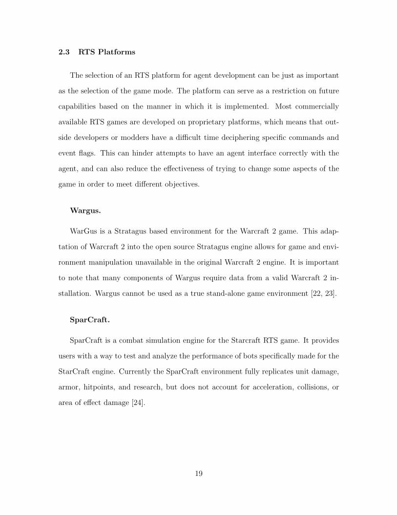
2.3 RTS Platforms
The selection of an RTS platform for agent development can be just as important
as the selection of the game mode. The platform can serve as a restriction on future
capabilities based on the manner in which it is implemented. Most commercially
available RTS games are developed on proprietary platforms, which means that out-
side developers or modders have a difficult time deciphering specific commands and
event flags. This can hinder attempts to have an agent interface correctly with the
agent, and can also reduce the effectiveness of trying to change some aspects of the
game in order to meet different objectives.
Wargus.
WarGus is a Stratagus based environment for the Warcraft 2 game. This adap-
tation of Warcraft 2 into the open source Stratagus engine allows for game and envi-
ronment manipulation unavailable in the original Warcraft 2 engine. It is important
to note that many components of Wargus require data from a valid Warcraft 2 in-
stallation. Wargus cannot be used as a true stand-alone game environment [22, 23].
SparCraft.
SparCraft is a combat simulation engine for the Starcraft RTS game. It provides
users with a way to test and analyze the performance of bots specifically made for the
StarCraft engine. Currently the SparCraft environment fully replicates unit damage,
armor, hitpoints, and research, but does not account for acceleration, collisions, or
area of effect damage [24].
19

Spring RTS Engine.
The Spring RTS Engine [25] contains many options that are useful to RTS re-
search. Some of the most important of these options are visualization, animation,
unit customization, and the fact that it is open source.
Visualization.
The visual capabilities of the Spring RTS Engine are an important factor to con-
sider when creating an agent that is meant to simulate theoretical military battles.
Unit models can be changed and the landscape terrain features can be modified as
needed. This allows for scenario modification and customization, which in turn allows
a user to test potential strategy and tactical outcomes in a simulated environment
Animation.
The animation portion of the Spring RTS Engine, and any RTS engine, provides a
visual feedback to the user of how battles progress through time. While simpler simu-
lation programs may be able to provide a numerical analysis of a battles conclusion or
state at a specific time, an animated progression allows users to have a direct feel of
the flow of battle. This allows a user to learn and eventually hypothesize the outcome
of certain situations and change their strategic or tactical decisions as needed.
Unit Customization.
One of the most powerful capabilities that the Spring RTS Engine brings to the
table is the ability to generate and implement new unit types. This allows further
customization of the battlefield in order to replicate an expected encounter. The
capabilities included in the Spring RTS Engine’s code go as far as introducing a
unit’s turn rate, turret turn rate, and attack rating against different types of targets.
20

This provides a means for planners to input specific unit capabilities based on current
intelligence.
Open Source.
The most useful aspect of the Spring RTS Engine with regards to applying an
externally generated AI agent is the fact that it is open source. As an open source
program, all code pertaining to the program is readily available and once deciphered
can be used to improve the application of any agent. The open source factor also
includes the ability to create new interrupts or event flags which a user can build to
occur at very specific situations - further improving the customization of this software.
2.4 Strategic Decision Making
The concept of strategy encompasses the goal of achieving a set objective or ob-
jectives while being restricted by a set of constraints. The decisions made in the
development of a strategy are generally higher level, with a leader’s choices affecting
a large amount of people or resources. Strategy can be used in many environments,
be it business management, military engagement, or personal finance. In warfare,
strategy can be used to accomplish a military leader or country’s goals. The goals of
military encounters change based on the strategist, with leaders such as von Clause-
witz establishing that victory in a battle should be determined by decisive battles
of annihilation or a slower series of battles of attrition, effectively tying victory di-
rectly to the remaining military power of the opponent [26]. Other leaders such as
Antoine-Henri Jomini focused instead of the geometry of battle, attempting to find
a method to compare military strategic decision making to a mathematical formula
or ideal series of decisions. In Jomini’s approach victory did not require destruction
of the enemy - victory can also be gained by sufficient acquisition of territory or re-
21

Figure 5. RTS Strategic Planning Tree [5]
sources [27]. In either case, the objective of military strategy can be victory via the
destruction of enemy forces or the capturing of enemy territory and causing a rout.
Strategic Planning in RTS games.
The strategic planning of an RTS game covers the same objectives as a standard
military confrontation. In most RTS games the objective is complete destruction of
the enemy, with some versions describing victory as the elimination of any manufac-
turing ability or the conquest of a specific portion of the game map. These goals
are accomplished through the development and application of a series of construc-
tion actions, otherwise known as a build-order [5]. The build-order is responsible for
moving a player through various technological development stages and can improve
a player’s unit construction ability. For example, a technical level of 1 may allow a
player to build basic infantry, level 2 may introduce more advanced unit types such
as flamethrowers or heavy machine guns. Level 3 may build off this further and allow
the player to begin building larger assets such as tanks or other vehicles.
22

Figure 5 shows a variety of methods used to plan strategies in an RTS game.
The first distinction to make is the initial option between behavioral planning or
optimization. Behavioral planning is an approach based on either learned or trained
courses of action. The expectation for this type of strategic planning is that the agent
is provided a set of data that represents expert players decisions on build orders. The
agent takes this data, develops a case based reasoning methodology of what to build,
and utilizes this to mimic expert players. A potential fault in this method is the fact
that “expert” is a very loosely defined term in the RTS world, and that an agent may
not be effective against opponents using unknown strategies [5].
The remaining path in figure 5 represents optimization via performance based
metrics. The thought on this section of the tree is to ignore the concept of providing
an agent with external data based on expert play, and instead to allow the agent to
create its own decisions by maximizing or minimizing a series of functions that provide
a value to the current state of a game. Given a suitable function an optimization based
strategy can play at the same level or better than expert level players, but has the
issue of an increased level of computational time [5].
2.5 Tactical Decision Making in Combat Scenarios
If strategy is the overall plan made before approaching a specific problem, then
tactics is the series of smaller decisions made to fulfill the strategy. Tactics represent
the actions and specific utilization of resources in order to make progress towards
completion of a specific goal or objective. Tactics can change based on the situation
at hand. In military encounters tactics encompass the formation of units, position
of forces, and manner of attack. Tactics can take into account choke points and
environmental aspects. In short, if a strategy is to perform a task, the tactics define
how exactly that task is performed.
23

Figure 6. RTS Tactical Planning Tree
Tactical Planning in RTS games.
Tactical decision making in an RTS game focuses on the micromanagement of
individual units or groups of units. Micromanagement is an extremely important
aspect in competitive StarCraft play, with top earning professional StarCraft player
JaeDong stating that in StarCraft: Brood War his ability ability to control the mi-
cromanagement “made me different from everyone else in Brood War, and I won a lot
of games on that micro alone.” . He then continues to say that micro is more impor-
tant in StarCraft II than it was in StarCraft: Brood War [28]. These statements by
one of the top players in the professional RTS world show that the ability to control
the micromanagement of units is important, and that future games may increase the
requirement of mastering this skill set. Micromanagement includes movement deci-
sions, where to attack, how to attack, and how to maneuver in battle. Movement
decisions focuses on the distribution of forces at the beginning of an attack. Units
can be grouped tightly together or split up in various smaller groups in order to en-
able flanking or ambush attacks. The decision on where to attack could be a players
decision to wait for enemy units to pass through a choke point which would maximize
the ratio of friendly units to enemy units engaged in the fight. How to attack is the
24

method of choosing distinct targets for each unit participating in combat. Finally the
maneuvering during combat references tactical retreats or “kiting”, which is when a
player moves within range to fire a volley and then retreats out of the opponents range
to reload. The research done in this paper seeks to optimize the targeting portion of
tactical decision making.
Figure 6 presents a variety of target acquisition methods available to AI agents.
The simplest type of decision making tool is a strict scripting method. These types of
methods analyze the current status of enemy units and makes a decision based on a
single metric. These techniques are very fast, but are open to exploitation by players.
The non-scripted methods of attack involve using similar methods to the strategic
development options shown in Figure 5. The Monte Carlo Tree Search (MCTS)
method analyzes the current state of a battle as if it is a static turn based game such
as chess. It takes the time to determine potential outcomes and provides a scalar
weight to each option. Another method of using a non-scripted learning method is
to provide a set of expert data to the agent or allowing the agent to run through
multiple simulations to generate its own data, as in the strategic decision making
process. This expert data can be used to have the agent mimic an expert player’s
decision methods. Finally, an MOEA can be used to create an attack solution based
on currently available information that would assign each unit a target with the goal
of outperforming the capacities of a human player.
2.6 Previous AFIT Developments
The agent being modified by this research topic has been in development for four
years, with Jonathan Di Trapani’s work in 2012 and Jason Blackford’s additional
work in 2013 serving as the most recent improvements. The objective for each step
of the development of the agent is to build on and improve a customizable RTS AI
25

agent that can be used as a means to train military members in strategic and tactical
decision making.
Adaptive Response - Weissgerber’s Agent.
Weissgerber’s work in 2010 created an agent that is capable of reacting to the
current situation of an RTS game by analyzing and acting on a subset of “features”
which are capable of encompassing the the current state of the game [29]. Weissger-
ber’s research culminated in an agent capable of outperforming the scripted agents
that faced it by analyzing those scripted agents’ previous performance and developing
an active counter strategy. This counter strategy is 100% effective against the tested
strategies, quickly analyzing the current state of a game and choosing decision paths
which led to “win” states by optimizing the state of the “features” used to represent
the game’s status.
Strategy Optimization - Di Trapani’s Agent.
Di Trapani’s agent seeks to develop a means of identifying and countering an
incoming wave of enemies [6]. This research is a continuation of the work performed
by Weissgerber [29] and works to build a variety of different strategies to determine
the effectiveness of each in various scenarios. In his work Di Trapani determines
the advantages and disadvantages of each strategy tested against all other tested
strategies. The purpose of this initial set of experiments is to determine the counter
to each strategy on each tested map. Once these results are compiled, Di Trapani
tests various classifiers that can be used to determine the enemy’s strategy given a
limited set of data. The purpose of this classifier is to allow the agent to hypothesize
an enemy’s strategy and start building the counter strategy. The result is a distinct
26
record of advantageous and disadvantageous options to choose based on the enemy’s
strategy selection.
Build Order Optimization - Blackford’s Agent.
Capt Blackford builds on the work developed by Capt Di Trapani by creating a
method to optimize the strategic decision making done in the initial stages of a game.
His agent, the Build Order Optimization (“BOO” for short) uses a MOEA to optimize
the build order for a given side. The MOEA selected has three objective functions.
The first function seeks to minimize the number of steps required to transition from a
current state to a desired state. For this first objective, the duration of all actions are
equivalent. The next objective function used represents the amount of consumable
resources required to move from a current state to a desired state. This objective
does not have uniform costs like objective 1, so objective 2 is able to generate a
more specific solution. The final objective simply takes the time requirements of each
action in a solution string and compares them to each other. The goal of this third
objective is to minimize the time required to complete a build order, otherwise known
as a makespan [5]. The end result of Capt Blackfords research is a MOEA based build
order modification tool that is capable of out-manufacturing bots currently available
for the Spring RTS Engine.
Tactics Optimization - AFIT Agent Continuing Work.
One of the most difficult problems that has developed through continuous im-
provement on the AFIT agent is the understanding of the code. As with any project,
understanding another person’s code can be a difficult endeavor. In the case of the
AFIT agent this is exacerbated by the use of multiple managers through the AFIT
agent as well as the references to various Spring RTS Engine libraries written in both
27

Python and C languages. One approach to the current AFIT agent is to begin a
cataloging and reference building of how all of the agents work together. Other ar-
eas the agent is lacking is the fact that the agent currently requires full battlefield
awareness - it cannot be used with any sort of “fog of war”, as some of the basic de-
cision making requires the knowledge of the enemy commander location. The agent
can also be improved on tactical decision making since it uses a very simple scripted
algorithm to determine tactics in a battle. The agent can also be improved in the
base construction / manufacturing stage, as it is currently incapable of using multiple
construction units. In short the agent can be improved on almost all fields of play,
as human techniques and ingenuity create or demand consideration of new tactics or
strategies to counter currently used options.
2.7 Current Research in RTS Tactics Optimization
The current research environment for tactical decision making in RTS games is fo-
cused primarily on single objective evolutionary algorithms or making decisions based
on AI learning techniques. Many researchers also focus heavily on applying their tech-
niques to the game of StarCraft. This is likely due to the widespread knowledge of
the game, as well as the availability of AI competitions that a researcher can use to
provide measurable metrics to grade their agent’s performance. Robertson and Wat-
son describe StarCraft as “a canonical RTS game, like chess is to board games, with a
huge player base and numerous professional competitions” [11], in their 2014 analysis
of current RTS AI. Chapter 2 of Roberson and Watson’s review covers tactical AI in
depth, leading to three major tactical decision making techniques prevalent in current
AI research. These techniques discussed in this review are Reinforcement Learning,
Game-Tree Search, and Monte Carlo Planning [11]. Other methods of RTS tactical
decision making include subjects such as genetic algorithms and fuzzy logic decision
28

making, but these types of methods are typically used in the strategic decision making
level [30].
Reinforcement Learning.
Reinforcement learning is the concept of providing feedback to the agent based on
the outcome of a specific scenario. One example of this is to have a Markov decision
tree with no weights on each decision - every probability is equal. The agent traverses
the tree until it reaches an end point. If the end point is a win, the agent provides a
positive weight score, if the end is a loss then the agent instead provides a negative
weight or a weight of zero. This weight is back-propagated through the chain of
decisions the agent used to reach the final point. This back-propagation skews the
probabilities for decision points along the tree search, which affects future runs of the
algorithm. This action of testing and then skewing the probabilities eventually leads
to an agent with a decision tree that is heavily weighted towards winning decisions
[31].
Wargus and Case Based Reasoning.
The research performed by Aha et al. is focused on applying the same case-
based reasoning approach used in chess and other genres to the RTS environment.
The RTS environment used for this research is the Wargus platform, an Strategus
based representation of the original Warcraft 2 environment [22]. The result of Aha
et all’s combination of Case based reasoning to tactics/strategy pairings shows that
case based reasoning is capable of performing very well in the realm of RTS games.
After 100 games the case based reasoning agent achieves an 82% win rate, a noticeable
improvement from the original 23% win rate. Aha et al.’s research shows that learning
29

techniques are extremely viable in RTS environments as long as enough learning time
is provided against specified opponents [32].
Game-Tree Search.
A game-tree is the representation of a game and its future states as a tree diagram.
The current state is the root node, and each action available at the root node serves
as a branch that goes to a new leaf node representing the result of the action being
taken. Game tree search methods seek out ways to exploit this tree comparison to
find a good solution by limiting the search area by pruning unnecessary branches and
performing different search methods such as depth first search or Min-Max [31].
Starcraft, Sparcraft, and Game-Tree Search.
Churchill has performed numerous experiments into the use of AI techniques for
various RTS problem areas, and has also developed the SparCraft simulation of the
StarCraft RTS game [24]. He also organizes the AIIDE Starcraft AI competition
[14], and has worked with others in order to provide a level of analysis of current
generation RTS AI agents used in these competitions [33]. His own research into
the realm of RTS tactical decision making addresses the use of modified game-tree
searches to optimize the search process [13, 34]. These methods focus on speeding up
the search by trimming “bad” decision areas off of the search tree early on, and more
searching “good” branches more deeply.
Monte Carlo Planning.
The Monte Carlo Tree Search (MCTS) is an approach to tree search problems
by utilizing a Monte Carlo decision making process [35]. A tree search is a search
methodology where various states in a problem can be represented as nodes, each
30

node other than the root node must have a parent, and each parent can have multiple
children based on what decision options are available at the parent node. The search
evaluates each child and eventually determines an optimal course of action based on
the scores. The final solution is the path that leads to the best solution.
The Monte Carlo decision making methodology is a semi-random way of choosing
a solution. The idea is that if the average outcome of a decision at a specific point
(i.e. parent node) is known, then the better choice should have a higher probability
of being chosen. This is not always chosen, however, as sometimes the choice with
a lower win probability can have a higher payout at the end. This balance between
best choice and still choosing apparently sub-optimal solutions is why this search is
semi-random. The choice itself is random but the weight given to each potential
solution is weighted by the currently known value of each choice.
The MCTS combines the tree search and the Monte Carlo algorithm in a way
that is able to use the benefits of both systems. First off, the tree is started from
an initialized root node. This node represents the state of the system before any
decisions are made. From this node, a choice is made on the next step according to
a Monte Carlo based decision method. At the initial state all perceived payouts are
the same so the first decision is completely random. Once a new decision is made,
the remainder of the solution string is generated randomly and then the solution
generated is scored. This score is back propagated to the decision point, and the
payout weight at that point is modified. The search is then reset back to the root
node and the next search is performed with the new weight scales affecting the Monte
Carlo decision. This process is repeated until the entirety of the search tree is searched
or an artificial search interrupt is engaged. When the search ends the path to the
best child node found is given as the optimal solution.
31

Genetic Algorithms.
Genetic algorithms work by generating a population of solutions and analyzing
each member of that population with regards to a certain objective function. The top
performing members are selected and combined to create a second population which
is also analyzed against the fitness objective. The top performing members of this
second population replace the worst performing members of the original population
and the process is repeated. Each combination of populations is referred to as a
generation, and genetic algorithm run times are typically limited by population sizes
and generational limits.
Planet Wars and Genetic Algorithms.
Fernandez-Arez et all associate the genetic algorithm against the RTS game Planet
Wars in their research towards the 2010 Google AI Challenge. Planet Wars is a simple
RTS where a player is assigned a number of planets each with their own starting
units. Players must then utilize their fleets to conquer other planets and increase
unit production. The game is largely about expansion by conquering neutral planets
in the first stages of the game, and then evolves into tactics based combat as the
two players battle to take each others territories in the later stages of the game. The
results of the research show that a properly attuned genetic algorithm can be used to
create a high percentage win rate, but a poor choice of objective can actually work
against the AI agent and result in a higher loss rate [36].
Computational Agent Distribution.
Another important factor to consider in the construction of an AI agent is the
method the overall framework is built. Many researchers utilize a single agent design
that aims to have a single algorithm develop a solution to many aspects of the RTS
32

game. The AFIT agent is instead built using the modified technique introduced
by Weber et al. [37] for their StarCraft EISBot. This type of agent is actually a
compilation of many different agents - each individual file responsible for their own
area. In his paper Weber discusses that his agent has separate managers for Strategy,
Income, Construction, and Tactics. The AFIT agent built off of this initial design
plan has its own separate managers: Attack, Defense, Unit, Building, and Economy.
Each of these agents are able to prioritize and act on a different set of goals in
order to help offset the restrictions caused by the No Free Lunch (NFL) theorem.
This theorem states that no algorithm is optimal in all situations. The splitting of
an agent into multiple managers allows each manager to be separately customized,
which can provide better, faster searches in a smaller domain space.
Hierarchical Control of RTS AI.
In their 2014 paper, Stanescu et. all introduce a method of controlling combat in
RTS games by generating a hierarchy of agents to control units on the field according
to various objectives. The purpose of this model is to create a situation where some
agents are on the “squad” level which control individual units to accomplish a set
objective. These units fall under the control of other agents which have a “comman-
der” level of authority which seeks to accomplish an overall strategy by assigning
squads particular tasks. This split up of authority and decision making results in
many smaller searches being performed instead of a single solution being sought for
every unit on the field. This approach to RTS decision making is proven to have its
benefits, especially in large combat scenarios where other search methodologies such
as tree searches are overwhelmed by the sheer number of potential outcomes [38].
33

Figure 7. Example Pareto Front with Different Population Sizes (5, 10, 20, 50)
2.8 Multi-Objective Evolutionary Algorithm Tactics
The effort described for this research is a novel approach to the tactical decision
making problem area, as it utilizes a variety of MOEA methods to determine the best
targeting solutions faster than humanly possible. While current research primarily
focuses on single objective evolutionary algorithms or applying various learning tech-
niques and foresight, this research aims to create and test a methodology that is
capable of generating a “good enough” solution using data that is currently available.
The process involves testing various MOEAs under different parameter settings and
then choose the option with the best resulting Pareto front as the example to bring to
on line testing. The hypothesis is that a properly programmed MOEA finds an opti-
mal set of tactical targeting decisions that maximizes damage output and minimizes
wasted firepower.
2.9 Multi Objective Evolutionary Algorithms (MOEAs)
Multi Objective Evolutionary Algorithms are methods of solving problems by an-
alyzing the potential results with regard to a variety of objective metrics [7]. While
a single objective search focuses on optimizing a particular equation or metric within
a set bounds, MOEAs are capable of finding multiple solutions that provide a range
of outcomes based on the weighting of the objectives used. This range of data points
which scale the different resulting scenarios resulting from differently weighted ob-
34

jectives is known as the Pareto front. The Pareto front consists of a set of optimal
solutions that maximize the evaluation of a series of solutions based on which ob-
jective is assigned most important, least important, and every objective in between.
Each axis of a Pareto front is represented by a separate function. The front serves to
provide the user with a visual method of showing how the weighting of each objective
value affects the overall outcome of the algorithm [39]. An example of the Pareto
front can be seen in Figure 7 [40].
Nondominated Sorting Genetic Algorithm (NSGA).
The first algorithm to be discussed and used in this experiment is the Nondom-
inated Sorting Genetic Algorithm (NSGA). Currently NSGA-II [41] is the most
popular version of this algorithm used in MOEA software. The NSGA algorithm
works by first randomly generating an initial population of potential solutions. Each
of these solutions are then analyzed based on the objective functions set in the prob-
lem. Once all members of the initial population are analyzed they are ranked based
on their level of pareto dominance. The more dominant members of the population
are weighted higher than the non-dominant members of the population. The mem-
bers of the population are then combined, with the more dominant solutions having
a higher probability of being chosen for combination to create new members of the
population. Once these new individuals are generated they are also measured against
the objective values stated in the algorithm. The new members of the population are
then combined with the old, and the best set are maintained for the next generation.
It is important to note that there is a crowding factor - multiple individuals with
very similar objective values are not saved in order to maintain a certain level of
diversity in each generation. This process repeats for each generational instance in
the algorithm until a final champion individual is found [39].
35

Strength Pareto Evolutionary Algorithm (SPEA).
The original version of the Strength Pareto Evolutionary Algorithm (SPEA) was
developed in 1999 and aimed to combine many previously popular MOEA techniques
into a single new algorithm [42]. The SPEA algorithm stored non-dominated solutions
externally, used the concept of Pareto dominance to assign a scalar fitness value to
each individual, and performed clustering in order to reduce the number of non-
dominated solutions within the current generational solution set without negatively
impacting the Pareto front. The algorithm works by generating an initial population
P and an empty non-dominated set P ′. It then copies any non-dominated members
of P into P ′. If these new members of P ′ dominate or are dominated by existing
members of P ′, the dominated solutions are removed. If the number of members in
P ′ exceeds the maximum population size, then P ′ is pruned. Once the size of P ′ is
less than or equal to the maximum population size, the fitness for each member of P
and P ′ is calculated, members from both are taken and then used to create the next
generation. These steps are repeated until the maximum number of generations are
calculated.
The unique aspects of the SPEA are the fitness evaluation functions and the
clustering function used to trim an overfull P ′. The first step in this analysis is
to generate the scores for each member i ∈ P ′. Each fitness score, or strength is
evaluated according to the formula si = nN+1
, where N is the size of P and n is the
number of members in P that the point i ∈ P ′ dominates. Once this is accomplished
for every member in P ′, the algorithm then computes the fitness for each member
j ∈ P . The fitness of j is evaluated by summing the score of each point iinP ′
that dominates j, and then adding one. These evaluations are performed in each
generational computation, with the consideration that a lower fitness value leads to
a higher probability of being chosen for combination to create the next generation.
36

The final evaluation that takes place is the clustering function, used to trim down the
non-dominated set P ′. This function works by dividing each member i ∈ P ′ apart
into a set of clusters. If P ′ is overfull, the algorithm determines the overall distance
between each cluster. The nearest two points are then merged together into a single
cluster. This repeats until the number of clusters equals the maximum population
size. Once this is done a single solution from each cluster of size larger than one is
chosen as that clusters representative on the pareto front, and the other members of
that cluster are discarded.
Strength Pareto Evolutionary Algorithm 2 (SPEA2).
The SPEA2 is a continuation of the development used to create the SPEA [43].
The overall process used in each generational computation is largely similar to the
one used in the SPEA. First, an initial population set P0 is created, with a blank
set P ′0. An additional variable t = 0, which represents the current generation, is also
created at this time. Once the set is created then the fitness values of each member
of Pt and P ′t are calculated. All non-dominated members of Pt and P ′t are copied
into P ′t+1. If P ′t+1 exceeds the current population limit, then it is truncated. If the
generational limit has not yet been reached, then the members of P ′t+1 are combined
via binary tournament selection in order to create the next generation. This process
repeats until the generational limit is reached.
The first difference in the calculations performed in Strength Pareto Evolutionary
Algorithm 2 (SPEA2) is the fact that every point in P and P ′ are assigned a strength
value. In the SPEA, the fitness value of a point in P is simply the sum of the
strength values of the members in P ′ that dominated it. This could potentially lead
to numerous points in P having the same value, and a sub-optimal one of these being
selected for future combination. SPEA2 fixes this by assigning every point currently
37

in consideration a strength value, and then following the old process of a fitness value
for any given point i being the sum of any points j 6= i that dominate point i. This
creates a hierarchy of dominated points, so that a point that is only dominated by
the points in P ′ has a higher chance of being selected for combination than a point
in P that is dominated by points in both P and P ′. The pruning operator of the
SPEA2 has also been modified. The first new capability of this operator is to always
maintain the furthest points on the pareto front in order to ensure that the front
is always as long as possible. The second modification is to sort through the entire
solution set P ′t+1, find the closest two points, and remove the point of that pair that
does not increase the maximum distance between the pair and adjacent points. These
two operations ensure that the resulting pareto front is more uniformly distributed
across the entirety of the pareto front.
Non-Dominated Sorting Particle Swarm Optimization).
The Nondominated Sorting Particle Swarm Optimization (NSPSO) algorithm is
an application of the Particle Swarm Optimization (PSO) methodology to a multi-
objective landscape [44]. This algorithm combines concepts from PSO and Non-
dominated Sorting Genetic Algorithm II (NSGA-II). First, an initial population is
developed, each member of the population has a randomized starting velocity within
a previously set boundary. Each of the members of this population is then analysed,
and the non-dominated members are copied into a separate list. Once the list of
non-dominated solutions is completed, the algorithm chooses one member from this
non-dominated list as the best, and uses this as the global best option for the rest
of the calculations in this generation. The rest of the operations of the PSO work
as normal, with the other members within the population changing their vector and
velocity to move towards the current personal best and global best members in the
38

population. This results in an MOEA that gradually clusters its solutions near the
best solutions, leading to a more intensive localized search while sacrificing the ability
to search the entirety of the available landscape.
Other Multi Objective Evolutionary Algorithm Options.
There are numerous other methods of solving multi-objective problems, as any
algorithm can be modified to more closely fit a specific problem at hand. This mod-
ification limits the use of this now customized algorithm for the purpose of solving
other problems so there is a trade-off between having a generic algorithm that can be
used on many problems or creating a custom problem suitable for a single problem
[45, 46].
Pareto Front Indicators.
The multiple ways of deriving a Pareto front leads to the problem of the compar-
ison of the results of one MOEA to the results of a separate option. For each specific
problem, there is an MOEA that works the best, and one that does not work as well.
This is known as the “No Free Lunch” theorem, which in essence explains that there
are always optimal and sub-optimal algorithms available to solve any given problem.
There is no such thing as a universally optimal search algorithm [47]. The goal of any
Pareto front indicator is to judge the Pareto result from a given MOEA and provide
a means to compare that result to the result from a different MOEA.
Hyperarea / Hypervolume.
The hypervolume (HV) or Hyperarea (HA) method aims to maximize the area or
volume covered by a particular Pareto front. This indicator determines the volume of
39

an objective space that is dominated by any given set A with regard to a designated
origin point [48].
R - metrics.
R-metrics operate by using an external utility function to compare the results
of any Pareto front. Each point within the Pareto fronts being compared is put
through these utility functions and then the results can be used to provide a means
to determine which option is better. The results of an R-metric analysis between
Pareto fronts is heavily reliant on the metric used for the comparison, and the user
should also be aware that a single large outlier can offset numerous smaller differences
[48].
Generational Distance.
The Generational Distance (GD) method compares the results of a given MOEA
to the known best Pareto front available. Each member of the MOEA’s resulting
Pareto front is paired with the known best, and the total difference between the two
options is calculated. This results in a clear metric that can be used to determine
how close any given Pareto front is to optimal. The limitation of this indicator is that
the user must first know what the optimal Pareto front is for a given problem [48].
ε - indicator.
The epsilon indicator operates by attempting to minimize the value ε that causes a
set B that is dominated by another set A to instead weakly dominate A. This can be
visualized as determining the amount of error that, if added to a substandard option
B improves B to perform at least as well as the alternative A. This metric requires
two different sets to compare, and can show improved results if the true Pareto front
40

is known, as it then becomes a metric directly comparing distance away from the true
Pareto front [48].
MOEA Software.
The purpose of the MOEA software selection is to serve as a external framework
that the AFIT agent can access and use to determine an optimal course of action for
the controlled units to take. These frameworks can be accessed in different ways and
can come in a variety of coding languages.
jMetal.
One of the most popular MOEA frameworks available is jMetal (Metaheuristic Al-
gorithms in Java) [49]. As expected from the name, this framework is coded entirely
in Java and is capable of handling NSGA-II, SPEA2, PSO, and a variety of other
algorithms. It also supports numerous quality indicators such as hypervolume, gen-
erational distance, and inverted generational distance. This software provides a very
robust system with the means to analyze a variety of potential setups with regards
to MOEA performance and evaluation.
MOEA Framework.
MOEA Framework is another java library custom built to support MOEA problem
solving. This library supports numerous types of MOEAs, including the recently de-
veloped NSGA-III algorithm. It also supports numerous metrics to gauge the results
and performance of various MOEAs on a specific problem, and includes a pre-built
graphical user interface for easy translation of the results [50].
41

PyGMO.
Another MOEA evaluation framework is the python language based PyGMO
(Python Parallel Global Multi-objective Optimizer) [51]. Developed by the Eu-
ropean Space Agency (ESA), PyGMO is a powerful tool that takes advantage of
python’s malleability as a coding language. PyGMO integrates with some other pop-
ular python based scientific evaluation software, such as SciPy, NLOPT, and SNOPT.
While PyGMO provides an easy to understand structure to determine best results
and scoring, it does not have as much breadth as jMetal. Many of PyGMO’s built
in algorithms are focused on single objective evolutionary searches, and it currently
only provides hypervolume as a means to analyze the results of a given search.
ParadisEO.
ParadisEO is a C++ based framework for MOEA analysis that supports many
basic MOEAs such as MOGA, NSGA-II, and SPEA2. It also contains the capability
of using a variety of built in metrics and quality indicators such as hypervolume and
additive and multiplicative epsilon [52, 53].
Borg.
The Borg MOEA is a specifically coded program that utilizes a single custom built
algorithm. This algorithm seeks to measure the tradeoffs between different objectives
and modifies itself to run optimally for the problem at hand. The Borg MOEA is
coded in ANSI C. This MOEA is focused on attuning itself and modifying its own
parameters in order to achieve optimal analysis of a new problem. [54].
42
Others.
The list provided in Chapter 2.9 is only a portion of the software available that
has been built to address the analysis of MOEA problems. A much more intensive
list is maintained by Dr. Coello Coello which holds many libraries and frameworks
built for the analysis of a particular MOEA or problem of interest [55, 56].
2.10 Chapter Summary
This chapter provides a synopsis of many concepts and approaches used to plan
and accomplish the experimentation performed for this research. An overview of
the decision making process is provided, as well as a link to the analysis and use of
this process for its application to the RTS decision making problem. A variety of
considered RTS software platforms and MOEA libraries and environments are listed
in order to provide an overall view of currently available technology applicable to
this research. Finally, a comparison between strategic and tactical decision making
is shown, as well as a variety of different approaches to the tactical decision making
problem that have already been tested. The following chapters provide an explanation
and process of the newly generated MOEA based tactical decision making RTS AI
agent that is used to create targeting solutions in online play on an RTS environment.
43

III. Methodology of RTS Tactical Design
3.1 Introduction
As stated in Chapter I, the goal of this thesis research is to develop a decision
making element of an RTS game agent that utilizes MOEAs to make fast, optimized
tactical battlefield decisions. The research is segmented to accomplish three primary
objectives. First, the research combines external MOEA software with the previously
existing AFIT RTS AI agent [6, 5]. Once this integration is complete an offline sim-
ulation of combat is developed and used to test the performance of different MOEAs
to find which type of MOEA performs best with the RTS tactical decision making
problem, and which parameters maximize this performance. The best performing
MOEA/parameter set out of the tested options are coded into the AFIT agent and
tested against various scripted tactical decision making methods which serve as a
comparative basis to test the performance of the MOEA.
This chapter is decomposed in order to adequately describe the methodology of
each of the three primary phases. First, a brief high level description of the entire
experimentation process is provided, along with an analysis of the new software used
to perform MOEA analysis within the AFIT agent. The chapter then goes into detail
describing the purpose and process for each of the primary phases, development of
the problem, offline experimentation, and online experimentation, and details the
selection of the required metrics and analysis tools used to gather data. The chapter
concludes with a summary of all actions performed, and leads into Chapter 4. Chapter
4 expands on the information provided in Chapter 3 and provides a more detailed
explanation into the actual steps used to perform the research.
44

3.2 Overview of Research Approach
The purpose of this research is designed to test the capacity of MOEAs for use in
solving the RTS tactical decision making problem. To accomplish this task, MOEAs
with differing parameter settings are used to solve an offline simulation of a round
of combat in order to determine which search method performs the best in the tac-
tical decision making search landscape. This research and experimentation requires
analysis of multiple types of MOEAs, integration of MOEA software with the exist-
ing AFIT agent and Spring RTS Engine, and final evaluation of MOEA controlled
tactical decision making against scripted opponents.
The development in this thesis investigation has three distinct phases. In the
design phase, the objective is to combine the currently existing AFIT agent with
the PyGMO python library [6, 51]. This requires the development of a new MOEA
structure which represents a round of combat in the Balanced Annihilation mod [57]
of the Spring RTS Engine. Once completed, this customized structure is used exten-
sively in experimentation phase two, and is maintained in the online decision making
of experimentation phase 3. Experimentation phase two consists of testing of vari-
ous MOEAs and measuring their performance in solving the RTS Tactics problem.
Multiple MOEAs are used in this phase, which are chosen based on their differing
search techniques. Each MOEA is tested under a variety of population and genera-
tion limit parameters in order to gauge parameters’ effects on the performance of the
MOEA. The resulting performance of each MOEA in solving the RTS tactical deci-
sion making problem is decided based on an analysis of the generated Pareto front.
The most optimal MOEA should have a quickly expanding Pareto front, which should
depict a series of high-performing solutions being generated quickly [58]. Speed is a
critical factor in the RTS tactical decision making problem, as solutions quickly be-
come outdated due to a constantly changing battleground. Thus, the best performing
45

MOEA/parameter set is coded into the AFIT RTS AI agent and used as a test case
against a variety of scripted tactics. The performance of the MOEA based tactical
agent is tested against a new set of objectives, and the results are used to determine
the effectiveness of MOEAs as tactical decision making managers.
3.3 MOEA Software Selection
The PyGMO library is selected as the MOEA software for use in this research [51].
The PyGMO software allows for four dimensional Pareto front analysis while also
allowing use of the NSGA-II, SPEA2, and NSPSO algorithms [51]. PyGMO was also
coded in the python, which is the same language used to write the AFIT RTS AI agent
[6, 5]. Choosing a MOEA library with the same native language as the existing agent
allows for easier integration with existing code. Libraries utilizing other languages
would require additional development time which would have a questionable impact
on the overall performance of the MOEA based tactical decision making manager.
The purpose of this research is to prove the usability of MOEAs in the RTS tactical
decision making problem - complete optimization of this agent is not within the scope
of this research.
3.4 Design Phase 1 - Integrating Spring RTS & PyGMO
Phase 1 of the research includes the redesign of the existing AFIT tactical decision
making manager to allow for the integration of MOEA based tactical decision making
within the Spring RTS Engine. This phase begins with the analysis of the methods
the AFIT agent utilizes to initialize and perform combat maneuvers, and modification
of the agent to act on champion solutions resulting from MOEAs. A custom problem
representing the RTS tactical decision making problem is also developed and used to
test the performance of different MOEAs in Phase 2.
46

Figure 8. File layout for the Di Trapani (AFIT) Agent [6]
47

It is important to note that the integration of PyGMO into the AFIT agent is
complicated by the nature of the AFIT agent. The AFIT agent is developed by
a variety of students, each with their own coding styles. The integration of open-
source software into the AFIT agent requires a very methodical approach in order to
minimize potential code conflicts or errors.
AFIT Agent.
The agent modified for use in this experiment is the one developed by Di Trapani
in his 2012 thesis research [6]. His agent is actually a framework of multiple managers
that constantly communicate with each other throughout the duration of the RTS
game. This inter-dependency allows each individual manager to enact a different de-
cision making process that has been optimized for a specific role. The setup of the
original AFIT agent is focused on generation and utilization of series of strategic op-
tions chosen through various configuration files. The tactical control exists within the
group.py file in the current AFIT agent, but follows very simple scripted commands
and is able to make decisions based on a complete knowledge of the current state of
the battlefield. A list of the original file structure can be seen in Figure 8 and the
inter-connectivity is shown in Figure 9.
As shown in Figures 8 and 9, agent initialization begins with Agent. This file
calls on the UnitClass file in order to define all units to be used with a given game
type. Once initialized, Agent creates and links AttackManager, DefenseManager,
BuildManager, and idleEventFilter. These four files control the majority of systems
during gameplay. BuildManager utilizes EconManager and the Strategy in order
to generate a series of initial actions for the agent to follow. BuildManager is the
primary control system until units are generated. Once units are generated they are
added to Group, within DefenseManager. These units are used to defend the base
48

until they reach the appropriate army size defined within a set strategy. Once the
army is “complete”, the Group is passed to AttackManager, who presses an attack
on the opponent. This process continues until one side participating in the battle is
destroyed.
The AFIT agent initializes two files, agent.c and agent.py. These two files serve
as the starting points for future calculations - agent.c acts as the first step in the ini-
tialization of the AFIT agent, and establishes the connection to agent.py. Agent.py
then reads the configuration settings laid out for the system under test and estab-
lishes the primary managers - BuildManager, DefenseManager, and AttackManager.
The initializations cascade through the various other python files as shown in Figure
9. This co-dependence not only allows for each agent to independently control it’s
portion of the game, but also allows for the introduction of new managers - a critical
trait for the introduction of MOEA analysis to tactical decision making.
AFIT Agent Configuration Settings.
There are two files that drive the initial configuration of decision making methods
of the AFIT agent. These files are config.txt and strategyDefs.txt. Config.txt is used
in the initialization of the AFIT agent through the cdata.py code, an example of
which can be seen in Figure 10. The config.txt file has three sections: The game
run number, which game map will be used as the battleground, and the individual
player settings. The game run number is the least important of these options as it
serves only as a marker for naming the results of automated testing of the agent. The
map designation specifies which Spring RTS map should be loaded for a particular
experimental run. These maps must be created in order to match the requirements of
the Balanced Annihilation mod, which include things such as player start locations
and resource patches [57]. The final section in strategyDefs.txt is a number of rows
49

Figure 9. File connection structure for the Di Trapani (AFIT) Agent [6]
50

# Game run number - Used for automated game play
3
# Name of map to be used
ThePass
# Player 1 - Strategy - data collection - Tactics
p1 25v25 on default
# Player 2 - Strategy - data collection - Tactics
p2 25v25 on moea
Figure 10. Example for config.txt
Table 1. Layout of a Strategy in strategyDefs.txt
Variable Name Domain Description
Build Power Integer value [0,100] Percentage of resources for manufacturing capability
Economy Integer value [0,100] Percentage of resources for economic development
Defense Integer value [0,100] Percentage of resources for defensive structures
Units Integer value [0,100] Percentage of resources for units
Group Composition Non-negative integer for each unit type to be considered Size and composition of an ”attack group”
Initial Economy 2-tuple of integer values Initial economy required
equal to the number of players on the map. Each of these rows is further split into
three sections - a player designator, a strategic method of choice, and a binary data
collection variable. The player designator is something as simple as labeling the first
player “p1” and second player “p2”. The second option sets the strategic methodology
for the agent to choose which is further defined by strategyDefs.txt. The final binary
variable is a setting to determine whether or not a players actions should be saved
in an external file. If true the game saves the current state of a game in an external
replay file every five seconds.
Modification of the AFIT agent includes creating a new manager, MOEA, which
will be called on by Group in order to provide a series of commands during battle.
This new manager will rely on information provided by
51

The strategyDefs.txt file controls the flags that the agent uses to make building
and attack decisions. A description of each of the separate sections of the document
can be found in Table 1. In Di Trapani’s version of the AFIT agent, this file holds
numerous lines of strategies such as tank rush and anti-air [6]. Each line in a strategy
tells the agent how to allocate resources, how to construct an attack group, and how
to initialize an economy at the start of a game. The initial economy factor is the
first segment of the code that the agent carries out, as it establishes a foundation of
economic development that provides the resources for future play. The group compo-
sition is the portion of the agent that begins an attack. When units are created they
are placed in a group under control of defenseManager. When a group is “complete”,
or deemed equivalent to the string in the group composition value, it is handed from
defenseManager to attackManager and set to attack. At this point a new group is
created and any newly generated units are again assigned to defenseManager.
Both of the configuration files are modified in order to support the implementation
of tactical decision making. Config.txt is changed to manage a choice between vari-
ous tactical decision making methods as well as strategic options, and new strategic
definitions are added to strategyDefs.txt in order to support simulated experimenta-
tion. The specific changes and addition of new tactics to config.txt are described in
Appendix A
PyGMO.
PyGMO is a python based library which provides the capability to analyze various
problems via included optimization processes [51]. Each use of PyGMO requires the
initialization of a problem, selection of an algorithm, and evolution by populating an
“island”. A example is provided via of one of the tutorials on the PyGMO website and
is shown in Figure 11a [59]. This example shows how PyGMO solves a 50-dimensional
52

from PyGMO import *
# Initialize Problem
prob = problem.schwefel(dim=50)
# Select Algorithm to Solve
↪→ Problem
algo = algorithm.de(gen = 500)
# Generate Island for Initial
↪→ Population
isl = island(algo,prob,20)
print isl.population.champion.f
# Evolve the Population 10 Times
isl.evolve(10)
print isl.population.champion.f
(a) Code for PyGMO Example
(17643.0955597,)
(0.00063643016983401569,)
(b) Output for PyGMO Example
Schwefel minimization problem. As seen from the code any PyGMO initialization has
three main components: the problem to be solved, the algorithm used to solve the
problem, and the “island” that the population of potential solutions resides on.
In Figure 11a, the first line is responsible for implementing the PyGMO library.
The next line which initializes prob sets this variable as a integrated problem that has
been built into the PyGMO software, with the variable dim=50 setting the number
of dimensions to be implemented in the calculation. The analysis of a RTS game
environment requires a customized problem to capture the current battlefield situa-
tion. The next line sets the variable algo to the differential evolution algorithm with
500 generations. This is made possible by the algorithm.de set-up, where the de
stands for differential evolution. The last step is to build the population’s island.
The command island(algo,prob,20) creates an initial population of 20 members
53

that is then modified by the algorithm and problem via evolution. The best member
of the population can be found at any time via the isl.population.champion.f
command. The results of the two print commands included in Figure 11a can be
seen in Figure 11b. The first line in Figure 11b is the best member of the initialized
population of 20 members. The second line in Figure 11b shows the results after the
population has been evolved 10 times. Based on the definitions instantiated by the
variable algo, 10 evolutions of the island is actually 10 ∗ (gen = 500) generations, or
5, 000 generations. That is why the algorithm is able to find such a small end result
in only ten evolutions.
Custom Tactics Optimization Problem.
The utilization of MOEAs to solve the RTS Tactics Optimization Problem requires
the development of custom problem for use in the PyGMO RTS Engine. The problem
developed is loosely based on the build order optimization problem developed by
Blackford in the previous AFIT agent [5]. For the custom RTS tactical optimization
problem, each solution consists of a string with length equal to the number of agent-
controlled units in the army. Each position of this string holds a value between 0 and
the number of enemies in the battle. The position - value pair represents the target
for the agent controlled unit. An example can be seen in Figure 12, and the code for
this custom RTS tactics problem solution can be found in Appendix A.
Instantly Spawning Units in Spring.
Typically, unit creation in Balanced Annihilation requires the construction of ap-
propriate factories or barracks. This can require up to 15 minutes for an agent to
build up an appropriate number of units to test tactical decision making methods [6].
In order to speed this process, the online testing of phase 3 relies on “cheat” com-
54

Figure 12. Example Solution for 3 vs 2 Combat
mands built into the Spring RTS Engine. These cheat commands allow instantaneous
construction of units so that quick battles can be performed. The utilization of cheat
codes drops a single simulation time from 15 minutes to under 2 minutes. This pro-
cess of instantly generating units is critical for increasing the speed of online testing of
the RTS tactical decision making problem. Base development is unnecessary for tac-
tics testing and differing base development decisions between the two tested agents.
This may cause armies to be launched at different times, which negatively effects the
analysis of tactics performance by affecting battle location or army completion rate.
3.5 Design Phase 2 - Developing Off-line Simulations
Once the custom solution to the RTS tactical decision making problem is devel-
oped, it is used to analyze the performance of various MOEAs in an off-line envi-
ronment. An off-line environment is employed because a typical game of Balanced
Annihilation (BA) takes approximately two minutes, even when hastened by the in-
stant generation of units described in Section 3.4. Performing online testing of each
MOEA under each parameter setting is time prohibitive, so an offline simulation is
created which represents the first round of combat. This truncation is performed un-
55

der the logic that if a MOEA/parameter set is capable of creating fast, well performing
solutions in the first, most complicated, round of combat, then that set also chooses
fast, well performing solutions in less difficult situations. Now that the framework
has been developed, the next step is to actually choose the MOEAs and parameters
to utilize for tactical decision testing.
MOEAs Under Test.
The MOEAs chosen to be evaluated within this research are NSGA-II, SPEA2,
and NSPSO. These algorithms are chosen because they represent generic coverage
search methodologies in MOEAs. NSGA-II represents algorithms that utilize semi-
random combination of seemingly optimal population members. SPEA2 focuses in-
stead on the maintaining the spread between members in a particular generation on
the Pareto front. NSPSO gathers its population members towards expected good
decisions, which results in a more in-depth search in a small area of the Pareto front.
These three methods present a combination of random, spread search, and focused
search methods. This provides a baseline approach towards the analysis of differ-
ent search techniques on the RTS tactical decision making problem. Each of these
MOEAs are also readily available for implementation in the PyGMO code, which
speeds development time and integration with the Spring RTS Engine [51]. The pa-
rameters changed for experimentation are the population and number of generations
to evaluate. Population size options are 20, 40, 60, 80, and 100. Generational numbers
are 2, 3, 4, and 5. These options are chosen because they provide a ”good” coverage
of the utility of each MOEA while also providing a range of potential solutions that
are calculated within a couple of seconds.
56
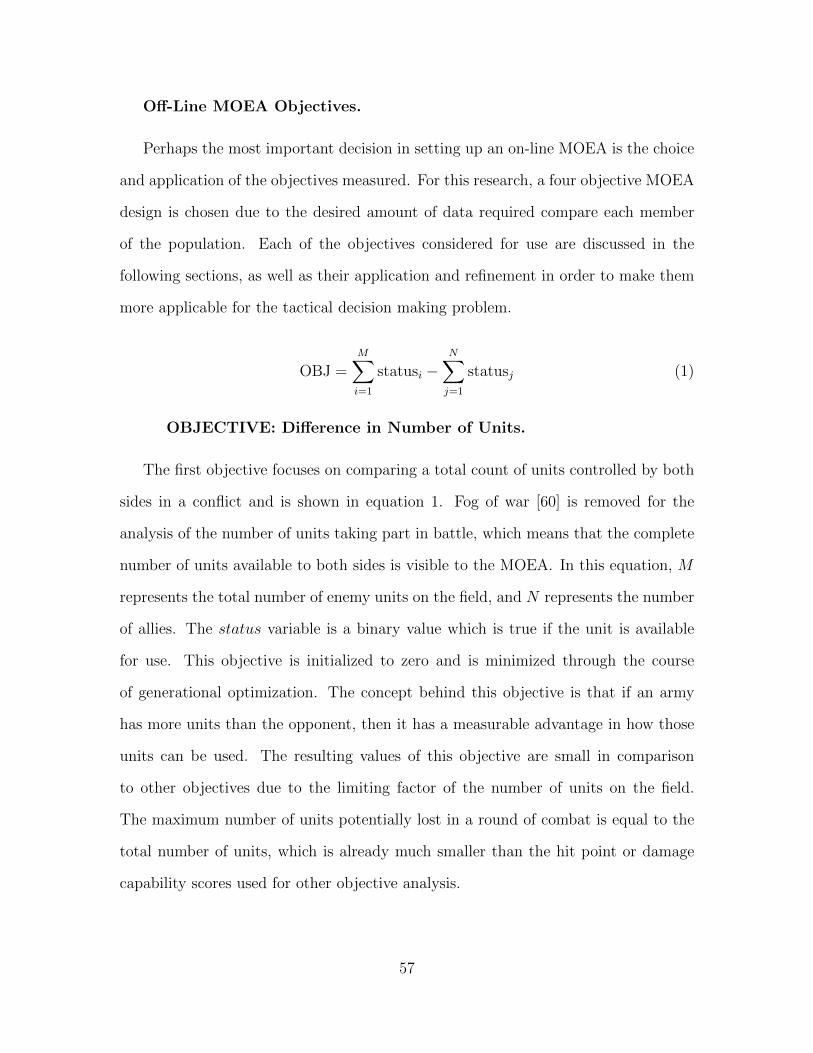
Off-Line MOEA Objectives.
Perhaps the most important decision in setting up an on-line MOEA is the choice
and application of the objectives measured. For this research, a four objective MOEA
design is chosen due to the desired amount of data required compare each member
of the population. Each of the objectives considered for use are discussed in the
following sections, as well as their application and refinement in order to make them
more applicable for the tactical decision making problem.
OBJ =M∑i=1
statusi −N∑j=1
statusj (1)
OBJECTIVE: Difference in Number of Units.
The first objective focuses on comparing a total count of units controlled by both
sides in a conflict and is shown in equation 1. Fog of war [60] is removed for the
analysis of the number of units taking part in battle, which means that the complete
number of units available to both sides is visible to the MOEA. In this equation, M
represents the total number of enemy units on the field, and N represents the number
of allies. The status variable is a binary value which is true if the unit is available
for use. This objective is initialized to zero and is minimized through the course
of generational optimization. The concept behind this objective is that if an army
has more units than the opponent, then it has a measurable advantage in how those
units can be used. The resulting values of this objective are small in comparison
to other objectives due to the limiting factor of the number of units on the field.
The maximum number of units potentially lost in a round of combat is equal to the
total number of units, which is already much smaller than the hit point or damage
capability scores used for other objective analysis.
57

OBJ =M∑i=1
HPi −N∑j=1
HPj (2)
OBJECTIVE: Difference in Remaining Hit Points.
The second objective considered compared the relative number of Hit Points (HP)
available to each side of the conflict. Like in objective 1, M is the number of enemy
units and N is the number of allied units. In this objective a pure sum of hit points
is taken and the difference between them is measured. The purpose behind this
objective is to attempt to measure the future survivability of an army in comparison
to enemy forces. If an army has more hit points then it has a higher probability of
surviving the next wave of attacks, which means that it is be able to continue firing
for a longer period of time and provide more damage to the enemy. This objective
is modified by having each unit’s HP represented as a ratio rather than a definitive
HP total, as some unit’s hit points can range into the thousands which skews the
objective analysis towards these four or five digit values and away from the smaller
objective values. This is represented in equation 2.
OBJ =
∑Mi=1 HPi∑M
i=1 statusi−
∑Nj=1 HPj∑N
j=1 statusj(3)
OBJECTIVE: Difference in Average HP per Unit.
The objective shown in equation 3 is a combination of the unit number and HP
difference objectives. First the total amount of hit points available to each army is
calculated, and then divided among the remaining units in that army. The purpose
of this objective is to create a glimpse into the survivability of each individual unit
on either side. This agent gives more weight to those armies with a higher average
58

HP value. This increases the optimality score of high HP armies, which have a higher
survivability rate in future battles.
OBJ =M∑i=1
damagei −N∑j=1
damagej (4)
OBJECTIVE: Difference in Remaining Damage Capacity.
The objective in equation 4 is a strict measure of the damage dealing capability
of the units remaining on the map. This objective is initialized to zero like other
difference based objectives. This measure subtracts all potential weapon damage that
allies units can perform, and adds damage capability of opposing units. The purpose
of this objective is to have allies units focus on destroying hard hitting enemies first,
thus reducing the strain allied units need to worry about in future stages of the battle.
This also allows allied units to focus on preserving their own heavy damage fighters
if mobility commands are implemented in the tactical agent.
for each enemy I in combat:
count = 1
for each ally J attacking enemy I:
Subtract count from objective score
count = count + 1
Figure 13. Code Representing Focus Fire Objective
OBJECTIVE: Focus Fire.
The objective shown in the pseudocode of Figure 13 is originally initialized to 0,
and decreases with regard to how many friendly units attack the same enemy target.
This objective checks each potential enemy in the list and subtracts an increasing
amount for each friendly unit attacking that target. The first unit is worth -1, second
59

is worth -2, third -3, and so on. Five friendly units attacking the same enemy would
subtract 5 + 4 + 3 + 2 + 1 = 15 from the objective. This objective is introduced in
order to increase the probability that friendly units focus on the same target. Prior
to the introduction of this objective, the MOEA is capable of maximizing damage by
spreading attacks randomly across all potential targets, and it is rare to get an early
kill due to damage across 5 enemies being equivalent to having 5 units fire on the
same enemy. With this objective allied units are able to severely damage, if not kill,
more units in each round of combat. This lowers potential enemy damage output and
also increases the likelihood of kills in future rounds.
OBJECTIVE: Damage / HP.
This objective is a modified form of the version discussed in Kovarsky and Buro’s
work [61]. In the original paper, the objective is
LTD(s) =∑u∈Ue
HP (u)dpf(u)−∑
u ∈ UaHP (u)dpf(u) (5)
where
dpf(u) =damage(w(u))
cooldown(w(u))(6)
This objective is modified to a more generic form in order to take into account a
base damage per hp for each unit by changing equation 5 as shown in equation 7
LTD(s) =∑u∈Ue
HP (u)damage(u)−∑
u ∈ UaHP (u)damage(u) (7)
This can be modified in order to achieve the end results from Kovarsky and Buro’s
paper, but it works sufficiently well in its current form in order to be able to distinguish
the importance of targeting low hp high damage units prior to high hp or low damage
dealing units. The focus of these equations is to have the agent focus more fire on
60

dangerous enemies with low hit points. If targets with high attack and low defense
are removed first, this not only removes enemy damage dealing capability but also
increases the speed and quality of future searches due to the reduced search area.
Objective Selected for Use in Offline Simulation.
The objectives selected for use in the offline simulation are the number of units,
the HP total, the damage capability, and focus fire. These objectives are selected due
to the uniformity of armies fighting each other - engagements for test are comprised
of only one type of unit. With this type of army composition the combination of HP
total, damage, and number of remaining units is expected to provide a precise view
of the overall health of the two armies after an attack. The focus fire objective is
added in order to enable friendly forces to heavily damage a few units rather than
distributing fire on many targets. This focus of damage either destroys enemy targets
within the first round or enables the search to have better, easier solutions in later
rounds of combat due to the existence of heavily damaged enemies.
While the focus fire objective skews the search area due to the fact that it is
capable of obtaining much larger values than the other averaged objectives, this offset
is mitigated by the inclusion of a variety of constraints within the custom RTS tactical
decision making problem. First, any damage dealt that brings an enemy past 0 hit
points is ignored, effectively negating the primary effects of that shot. Second any
expected damage to an enemy out of firing range is set to 0, which also negates any
seen benefit of focusing on enemies too far away. These two constraints work to
maximize focused fire while also preventing this objective from creating sub-optimal
solutions.
61

Measuring MOEA Performance.
The performance of each MOEA, population, and generational limit combination
is based on the improvement to the expansion rate of the Pareto front’s hypervolume
[39] over the course of time. This decision is made because the solution to the RTS
tactical decision making problem must focus on both speed and correctness. A larger
hypervolume provides a better “champion” solution, as the resulting Pareto front is
closer to the “true” Pareto front. The speed of solution is important because the state
of a RTS battle is constantly changing so a solution must be provided fast enough
to still be relevant. The objective of this metric is to determine which combination
of attributes leads to the fastest, best solution. In order to accomplish this task,
each MOEA is tested with a population of 20 and a single generation in order to
serve as a starting point. The hypervolume of these runs is used as the comparative
basis against the other MOEA / population / generation tests. For example, if the
NSGA-II algorithm is tested to find a hypervolume of x, then each subsequent test
uses the formula HV−xt
to determine the score of that combination, where HV is the
new hypervolume and t is the time required to complete the test.
3.6 Experimental Phase 3 - Developing On-Line Simulations
The objective of phase 3 is to take the best performing MOEA from phase 2 and
utilize it in a series of on-line runs to validate its performance against three commonly
scripted options. The MOEA selected for on-line integration is shown to out perform
the alternatives due to the results analyzed in phase 2.
RTS Tactic Methods.
There are three scripted tactical target decision making methods used to serve
as challengers to the best performing MOEA found in phase 2. These three scripts
62

are group attack closest, individual attack closest, and group attack weakest. These
options are chosen as options because of their use as a starting point of measuring
tactical performance in other researcher’s work related to tactical decision making
[13, 34]. Group attack closest is capable of balancing the number of units firing
during a round of combat while also maximizing the extent of focused fire. Individual
attack closest instead maximizes the number of units able to fire at the cost of focused
fire. Group attack weakest destroys damaged units quickly and removed their damage
dealing capacity from the battle as soon as possible.
Group Attack Closest.
The pseudocode shown in Figure 14 depicts the “standard” AI decision making
process for the AFIT agent. The entire code can be found in Appendix A The first task
the agent performs is to generate a blank matrix based map which holds the data for
all friendly and enemy units. This map is populated in the second for loop displayed
in the figure. The agent goes through a pre-generated list of enemy positions built
by the cdata.clb.getPositions command. These positions are assigned a point in
the matrix generated at the start of the code. Once all enemy positions have been
added to the targeting map, the central point of all allies forces contained in the
current group is found by the self. getCenterOfMass() command. This command
performs a similar task as the previously mentioned for loop, but instead takes all of
the X and Z coordinates for every unit in the currently controlled group and averages
them. The X and Z coordinates are chosen because the Spring RTS Engine treats
the Y axis as the vertical axis to denote altitude. Ground forces ignore altitude in
this version of the agent since range is a hard set parameter flying units likewise do
not need this axis as they operate at a constant altitude [6].
63

for each cell in map:
clear cell data
enemyMap = list of enemy units
size = length of enemyMap
unitIds = identification of each unit in enemyMap
enemyPositions = position for each unit in enemyMap
for each unit in enemyMap:
place enemy and corresponding data on correct position in map
xavg, zavg = center of mass of agent controlled units
if agent forces are flying:
attack enemy commander
else:
if enemy commander in line of sight:
attack enemy commander
else if building in line of sight:
attack building
else:
attack enemy in Line of Sight closest to (xavg, zavg)
if no enemies within line of sight
move towards enemy commander
Figure 14. Pseudocode for Default AFIT Agent Tactics (Group Attack Closest)
Once the average allied position and map of enemy locations have been built, the
agent begins sorting target priorities. The first task is to search for nearby enemy
buildings. If a building is closer than enemies then the building is set as the group’s
target marked by the enemy variable. If no buildings are within range the agent
then checks the size of the enemies list. If an enemy exists in this list the agent
determines the enemy unit closest to the coordinates (xavg, zavg) and set that as
64

the group’s target. The last step before firing is to determine if the chosen target
is actually within firing range. If the enemy is within range, the group attacks that
target. If no enemies are within visual range then the agent defaults towards telling
the group to move towards the enemy commander until enemies are encountered. This
repeats until the enemy commander is destroyed or the controlled group is completely
destroyed.
If a group is comprised of only air units, various if statements check for an “air”
designation. If this “air” setting is true, the agent ignores all tactics other than a
direct attack on the enemy commander [6].
Individual Attack Closest.
The algorithm for the Individual Attack Closest tactic is shown in Figure 15, with
the full code provided in Appendix A. This algorithm is a modification of the default
attack code shown in Figure 14, and takes place within the if statement checking if
the targeted closest enemy is within line of sight. This code differs in the manner in
which it engages the opposing force. Where the default code has every unit in the
group engage a single enemy, the individual attack closest tactic performs a sorted
search through all enemy locations. This search is performed by first determining
each allied unit’s location. This location is then saved, and a blank target list is
built. This target list is populated by comparing the allied unit’s location to every
enemy location on the map, with the result being stored as [distance, enemyId].
Once the list is completely populated a sort command is used to sort the target list
based on the first value, which is the distance. This sort puts the smallest distance
first, and then the agent assigns the unit to attack the enemyId associated with that
distance.
65

for each cell in map:
clear cell data
enemyMap = list of enemy units
size = length of enemyMap
unitIds = identification of each unit in enemyMap
enemyPositions = position for each unit in enemyMap
for each unit in enemyMap:
place enemy and corresponding data on correct position in map
xavg, zavg = center of mass of agent controlled units
if agent forces are flying:
attack enemy commander
else:
if enemy commander in line of sight:
attack enemy commander
else if building in line of sight:
attack building
else:
for each friendly unit
attack closest enemy
if no enemies within line of sight:
move towards enemy commander
Figure 15. Pseudocode for Individual Attack Closest
Group Attack Weakest.
The pseudocode for the algorithm controlling the group attack weakest tactic is
shown in Figure 16 and is very similar to the code used in the individual attack weakest
tactic (Figure 15). As with the other scripted tactics method, the full code can be
found in Appendix A. The selection of a target follows the same basic procedure,
66

for each cell in map:
clear cell data
enemyMap = list of enemy units
size = length of enemyMap
unitIds = identification of each unit in enemyMap
enemyPositions = position for each unit in enemyMap
weakest = 1
for each unit in enemyMap:
place enemy and corresponding data on correct position in map
if unit hit points < weakest hit points
weakest = unit
xavg, zavg = center of mass of agent controlled units
if agent forces are flying:
attack enemy commander
else:
if enemy commander in line of sight:
attack enemy commander
else if building in line of sight:
attack building
else:
for each friendly unit
attack weakest
if no enemies within line of sight:
move towards enemy commander
Figure 16. Pseudocode for Group Attack Weakest
assigning sort weighting on the enemy’s remaining HP instead of the distance between
67

a unit and potential targets. Once the sorting algorithm is complete, the unit is
assigned the target with the lowest sorted HP.
allies = []
enemies = []
for unit in friendly units:
append [ID, hit points, "alive", position, damage, range] to allies
for unit in enemy units:
append [ID, hit points, "alive", position, damage] to enemies
initialize RTS tactical decision making problem and initialize population
↪→ size
select algorithm for use with RTS tactical decision making problem and set
↪→ generation
initialize population
evolve population
select "champion"
for position in champion:
position (friendly unit) attacks value of position (target)
Figure 17. Implementation of MOEA in AFIT Agent
Multi Objective Evolutionary Algorithm.
The pseudocode for the MOEA based tactical manager is shown in Figure 17, with
the full code for this algorithm available in Appendix A. The algorithm controlling the
agent based on MOEA output is noticeably more complex than with the tactics based
on sorting. This method is based on building different arrays detailing information
for allies and enemy forces. The first task is to construct the allied array. This array
is built by first using Spring commands to determine the health and position for each
individual unit. This information is then used to build a line of the self.allies
68

Figure 18. Stumpy Tank
array, which includes the unitId, health points, alive/dead binary indicator, position,
damage potential, and attack range of each unit. Constant values are set for damage
and range in this research due to the fact that comparative battles are only using
a single type of unit, the Stumpy tank [62]. The stumpy tank’s model within the
Spring RTS Engine can be seen in Figure 18. Once the allied units’ array is built the
enemy array is built using a similar method.
The arrays are then passed to the custom problem built for the RTS tactical
decision making problem discussed in Section 3.4. Once the problem is set, the
algorithm, generational limit, and population limit of choice are applied in the moea,
gen, and pop fields, respectively. The population is then evolved, and the champion
string found. It should be noted that while in the example shown in Figure 11b
gives values due to the champion.f command, the champion.x command returns the
actual string that results in the best value. This string has i entries, where len(i)
is equivalent to the number of allied units on the field. The number at each position
j ∈ i is the target of i. These values can be used to have the attack command
associate each unit i with its target champion.x[i].
Measuring Battle Outcomes.
The on-line battles performed between various tactical methods can be used to
determine the effectiveness of those tactics. The strategy for each agent participating
in the battle is set to one which focuses on the development and construction of 25
69

Figure 19. Central Path of ThePass map on Spring RTS Engine
tanks, which are then sent to attack the other army. The map chosen for this is
ThePass (see Figure 19), which is a small multiplayer map on the Spring RTS Engine
which focuses on driving opposing forces through a central channel. This channel
can be used to force opposing armies to encounter and then begin attacking each
other, which is ideal for use in testing how different tactical decision making methods
perform against each other.
OBJECTIVE: Win Rate.
The first, and most important, metric that determines how well various tactics
perform against each other is a simple determination of which agent won the battle.
Winning is defined as the team who has forces remaining on the field when the other
side is destroyed. This metric can be used as an obvious measure to determine how
well an agent performs, but other metrics define the scale of the win based on other
factors such as time of battle and army health after combat.
70

OBJECTIVE: Time of Battle.
The next metric that is used to compare the differences between battles is the
overall length of time the conflict takes to resolve. The purpose behind this metric
is to determine how long an army is delayed by opposing forces. In RTS games, it
can be important to end a battle as quickly as possible in order to free up resources
to either return to base to defend against another attack or to continuously provide
pressure on the opposing player. This metric is measured in seconds, as that is the
smallest unit of time the Spring RTS Engine replay files can measure.
OBJECTIVE: Number of Remaining Forces.
Another important metric to consider is the number of remaining forces. In RTS
games, a unit with a single hit point can still serve either as a distraction to enemy
units or another platform to damage enemies. For this reason the number of remaining
units is used to determine how well various tactics perform against each other.
OBJECTIVE: Health of Remaining Forces.
The final metric that determines the grade of how well tactics perform against
each other is the sum of remaining hit points among the forces. This metric is aimed
at determining how well an agent has used its forces, and as a measure to determine
how useful surviving units are in future attacks. An agent that wins with a number
of severely damaged units is not expected to perform well in future engagements with
those units.
3.7 Chapter Summary
This chapter provides an overview of the design process and decisions made for
the execution of all three phases of this research. The chapter explains the three
71

phase approach that is used to determine the utility of MOEAs for use in solving
the RTS tactical decision making problem. Phase 1 consists of the representation of
the RTS tactical decision making problem in a MOEA solvable format, as well as the
selection and integration of a MOEA library into the Spring RTS Engine. Phase 1
also details the reasoning behind the selection of MOEAs and the pursuit of covering
a variety of search methods in order to be able to determine which search style works
best for the RTS tactical decision making problem. Phase 2 includes the selection
and implementation of objectives in the off-line evaluation of various MOEAs to
determine the performance of different search methods on the RTS tactical decision
making problem. Finally, Phase 3 takes the best performing MOEA from Phase 2 and
its parameters into an on-line evaluation within the Spring RTS Engine. This MOEA
is tested against three different scripted tactics and the performance is analyzed to
determine potential MOEA RTS tactical decision making. The next chapter provides
greater detail with regard to the experimental steps.
72

IV. Design of Experiments
4.1 Introduction
This chapter provides more information in the implementation of the steps de-
scribed in Chapter III. While Chapter III provided a high level view of the processes
used to perform the experiments gauging the effectiveness of MOEAs in an online
RTS environment, Chapter 4 aims to provide a step-by-step process and analysis into
how data is acquired and how selected objectives are implemented.
As in Chapter III, this chapter is split into a separate section for each primary
phase of research. The first section analyzes the process used to develop the inte-
gration between the selected MOEA libraries with the Spring RTS Engine. This is
followed by the procedure, code, and equations utilized to create and perform offline
simulation of combat in order to speed analysis of MOEA performance in battle. The
data found in the offline analysis is used to create an online tactical control manager
that is tested against three generic scripted tactical agents, and the results again
analyzed to determine MOEA performance within the RTS tactical decision making
problem.
4.2 Experimental Design
As discussed in Section 3.2, the research performed for this thesis effort is divided
into three distinct phases. Each phase results in the development of a tool required for
the next. These phases are sequential in order to construct an experimental process
capable of performing in depth analysis of the custom RTS tactical decision making
problem by relying on the output of previous phases.
Phase 1 begins with Di Trapani’s AFIT agent [6] and the PyGMO python MOEA
analysis library [51]. The objective of Phase 1 is to combine Di Trapani’s agent and the
73

PyGMO code together in a way which allows online optimization of an RTS battlefield
using MOEAs. This requires the creation of a customized PyGMO problem which
represents the RTS battlefield for on-line analysis. This problem is called within the
group.py manager in the AFIT agent by utilizing the PyGMO libraries. There are no
metrics associated with this phase as the result is just a code based representation of
a round of an RTS battle.
Once the battlefield simulation created in Phase 1 is complete, it can be used to
test the performance of the MOEAs of interest. Each MOEA is tested with differ-
ing populations and generational limits in order to gauge the landscape of the RTS
combat search area. The tested population sizes are 20, 40, 60, 80, and 100. The
tested generational limits are 2, 3, 4, and 5. These options are chosen in order to
cover the range available to the population and generation limit properties while also
constraining expected calculation time to be within on-line time requirements. The
metrics used for analysis of MOEA performance are focused on hypervolume maxi-
mization over time, as a solution needs to be made quickly but also correctly. A set
of objectives are selected from the list in Section 3.5 in order to provide enough de-
scription as to the optimality of the results of a battle. The MOEA which is capable
of maximizing the rate of hypervolume [39] expansion over time is chosen as the best
option for implementation in online testing. This MOEA is then coded into the AFIT
agent as a tactical option within the group.py manager.
Phase 3 is the final step of this research. In this phase the previous phases’ results
are combined to create an online tactical decision making tool which is implemented
within the Spring RTS Engine. This tactic is compared against three scripted oppo-
nents which are chosen as representatives of basic RTS combat design. Each combat
between various tactical decision making methods is statistically analyzed according
to the win rate, number of units remaining, speed of combat, and remaining HP.
74

4.3 Computer Platform and Software Layout
Online experimentation for this research is performed on the Spring RTS Engine
[25] version 0.98 using version 8.08 of the Balanced Annihilation mod [57]. The Spring
RTS Engine is selected due to the fact that it is open source and capable of heavy
modification for future testing. This level of modification allows for manipulation
of individual unit characteristics and features, as well as various cheat codes which
introduce ways to test very particular features of AI agents quickly through visual
simulation. The Balanced Annihilation mod allows for the use of many basic tenets of
standard RTS play such as resource gathering and easily identifiable unit types. This
mod is chosen as a representative of a generic RTS due to its implementation of two
types of resource gathering as well as having multiple specialized unit construction
facilities. The unit of choice for this experiment is the Stumpy Tank (see Figure
18, due to its arcing fire pattern, high armor score, and area of effect damage. The
tanks also have limited mobility and turn radius, along with a maximum turret swivel
speed, which adds complication to the decision making and allows more modification
of tactical decision making managers in determining an “optimal” fire pattern.
4.4 Design Phase 1 - Integration of Spring RTS and PyGMO
The integration of the Spring RTS Engine to the PyGMO code is handled through
the creation of a new manager in the existing AFIT agent. This new manager,
moea.py, is directly responsible for connecting the Spring RTS Engine and PyGMO
framework by utilizing PyGMO commands inside of the AFIT agent. The previous
version of the AFIT agent made combat decisions by relying on a set script within
the group.py manager [6]. The new version of the AFIT agent operates by having
group.py call on the custom PyGMO problem held within moea.py. The analysis
75

class ROUND(base):
def __init__(self, allies=[[0,0,0,[0,0],0,0],[0,0,0,[0,0],0,0]],
↪→ enemies=[[0,0,0,[0,0],0,0],[0,0,0,[0,0],0,0]]):
copy allies matrix into self.allies
copy enemies matrix into self.enemies
initialize PyGMO for a 4 objective minimization problem, with
↪→ solution length equal to the number of allied units
set bounds of output to [0, number of enemies-1]
Figure 20. Custom PyGMO Problem Created for Tactic Optimization (Initialization)
performed within moea.py returns a string of commands go group.py which is then
implemented within the Spring RTS Engine.
The integration of the AFIT agent and the Spring RTS Engine is accomplished
by using the custom PyGMO problem ROUND within the moea.py file. The problem
is initialized as shown in Figure 20. To begin, ROUND requires two arrays of data, one
for allied units and another for enemy units. The initialization of the problem also
requires that a “base” form of the allies and enemies arrays exist so that some data
exists during PyGMO’s population island creation. If these arrays are not set within
the definition of the problem then PyGMO attempts to deepcopy arrays that have
not been initialized, which leads to a program fault. The layout of each line in the
array of units is shown in equation 8. The data required by the ROUND class includes
a Unit ID set by the Spring RTS Engine, the number of hit points remaining for that
unit, a binary indicator representing if a particular unit is “alive” or “dead”, that
unit’s position, and finally the unit’s damage capability and range.
76

Unit = [Unit ID,HP,Unit Life Marker, [X Position,Z Position],Damage,Range]
(8)
Once data has been passed to the ROUND class, the arrays are copied into two local
variables self.allies and self.enemies. PyGMO is then initialized to prepare for
a 4 objective analysis of the input arrays, and each member of the output string is
bounded to a valid output command. The commands for this version of the RTS
agent are limited to attacking different enemy targets, so the number of potential
actions available to each unit is equal to the number of enemies on the screen.
Figure 21 shows the next step in the creation of a custom PyGMO problem -
analysis of a particular potential solution of a population. At this point within the
MOEA analysis, PyGMO has generated a population of solutions according to the
restrictions in Figure 20. The analysis of each member within a population starts
with the creation of two matrices for allied and enemy forces, astart/anew and
estart/enew, respectively. These matrices represent the initial state and the expected
resulting state from the analyzed solution. The values in anew and enew are modified
throughout the analysis in order to create data that is used for objective evaluation.
The first step in analyzing each solution is to check the resulting direct damage
from an attack wave. For each attacking unit the code confirms that the target is
within range and then reduces the targets HP by the attack value of the attacker.
If the target is within range, the target and any nearby enemies are damaged ap-
propriately. If this brings a unit’s HP below 0 then the unit is marked as dead by
setting their “alive” marker to 0. Once friendly forces fire, the algorithm calculates
the expected level of return fire from the remaining enemy forces. Once all damage
has been calculated the algorithm is ready to perform objective analysis of the enew
and anew matrices.
77

class ROUND(base): continued
# Begin objective analysis of solution
def _objfun_impl(self,x):
set starting matrices to self.allies, self.enemies
deepcopy start matrices to create end matrices
for each allied unit:
if target is within range:
deal direct damage
if other enemy is within area of effect range of shot:
deal indirect damage to that enemy
if enemy HP drops below 0:
enemy HP = 0
enemy = "dead"
for each enemy:
if enemy is alive:
select closest allied target
deal direct damage to allied target
if other allied unit is within area of effect range of shot:
deal indirect damage to that allied unit
if allied unit HP drops below zero:
allied unit HP = 0
allied unit = "dead"
Figure 21. Custom PyGMO Problem Created for Tactic Optimization (Calculation)
78

class ROUND(base): continued
initialize all objectives to 0
for each allied unit:
if allied unit is "alive":
subtract 1 from objective 1
subtract allied unit HP from objective 2
subtract allied unit damage from objective 3
for each enemy unit:
if enemy unit is "alive":
add 1 from objective 1
add enemy unit HP from objective 2
add enemy damage to objective 3
count = 1
for each allied unit:
if target of allied unit = enemy unit:
subtract count from objective 4
count = count + 1
return (f1,f2,f3,f4,)
Figure 22. Custom PyGMO Problem Created for Tactic Optimization (Objectives)
79

Figure 22 shows the final step of a custom PyGMO problem, the analysis of a set
of values and placement into a set of comparative objective values. The first step of
objective analysis is to initialize all objective variables to 0. This initialization must
be performed for each member of a population in order to prevent the results from a
previous member skewing the results for the remainder of the population. Once the
initialization is complete the effects of allied units are measured and subtracted from
the objectives 1, 2, and 3. As stated in Section 3.5, the objectives used are Units
Remaining, Difference in HP, Difference in Firepower, and Focus Fire. Once the al-
lied units’ effects on the battle have been computed and subtracted from objectives,
the results of the enemy units are similarly summed and added to the same three
objectives. The final step is to analyze objective 4, which evaluates the amount of
focus fire within a given solution. This objective is calculated by determining how
many allied units attack the same enemy. Each unit attacking the same enemy sub-
tracts (1 + number of units attacking that enemy from the objective). When all four
objectives have been measures the results are output back to PyGMO for population
modification. The entirety of this code can be found in Appendix A
4.5 Design Phase 2 - Offline Simulation
The experimentation within Phase 2 compares the performance of the different
MOEAs chosen for analysis, NSGA-II, SPEA2, and NSPSO. Each MOEA has a
different search mechanic, and this phase determines which general type of search
method is best for the tactical decision making search landscape. A description of
each of these MOEAs is given in Section 2.9.
80

Testing MOEA Parameters.
The Phase 2 experimentation is performed by comparing the results from NSGA-
II, SPEA2, and PSO MOEAs against each other in order to determine which search
method performs best in the RTS tactical decision making problem. These three
MOEAs are selected because they cover a variety of generic search procedures. NSGA-II
performs a semi-random search of the problem domain by combining the current best
performing members of the population in order to generate new populations. SPEA2
follows a similar search method, but discards potentially better scoring individuals
in order to ensure an even coverage of the Pareto front. NSPSO focuses entirely on
migrating the members of its population towards local and global optimal performing
members of the population. These three MOEAs therefore cover the random, spread,
and focused search processes. The parameters tested for MOEA optimization are
population size and numbers of generations to test through. The population sizes
tested are 20, 40, 60, 80, and 100. Generational sizes scale from 2, 3, 4, and 5. Alto-
gether this gives 20 different experiments per MOEA, or 60 different experiments total
for Phase 2. Each experiment is performed ten times in order to create a statistical
baseline for analysis.
Measurement Metrics.
There are a variety of different metrics available for testing the usefulness of a
particular MOEA on a problem. The metrics are known as Quality Indicators, and
can be Pareto compliant or non-compliant. If a solution set A better than a different
solution set B by weak Pareto dominance, then any metric that states A is at least as
good as B is Pareto compliant. Metrics that fail to maintain the relationship between
A and B are known as Pareto non-compliant [39]. A quick synopsis of many possible
options is listed below:
81

Error Ratio (ER).
The Error Ratio metric gives the ratio of members of the currently known Pareto
front vs. the members of the true Pareto front [39, p.255]. In other words, this metric
determines the percentage of PFtrue that has been found in the current generation.
A mathematical representation is available in equation 9 [39]. An ER of 0 signifies
that the current PFknown is the optimal Pareto front. An ER of 1 shows that there
are no current matches between any points in PFknown and PFtrue.
ER =
∑|PFknown|i=1 ei|PFtrue|
(9)
An issue with this quality indicator is that it requires PFtrue to be known, and as
such is not applicable in the problem discussed in this paper. The constantly changing
search landscape makes it impossible to nail down the exact optimal Pareto front.
Generational Distance (GD).
Generational Distance is another quality metric that compares PFknown to PFtrue.
This method compares the overall distance between the true Pareto front and the
currently available Pareto front. A mathematical representation is shown in equation
10 [39].
GD =(∑n
i=1 dpi )
1p
|PFknown|(10)
An issue that arises from the use of this indicator is that it is not Pareto compliant.
A Pareto non-compliant indicator can potentially mistake option B as being better
than option A in cases of weak Pareto dominance. Therefore generational distance
has the chance of showing incorrect optimal Pareto fronts due to the inherent method
of comparison.
82

Hyperarea / Hypervolume.
Hyperarea, otherwise known as hypervolume for Pareto fronts involving more than
two objectives, attempts to equate the multidimensional area or volume covered by
a given population of potential solutions. This is a Pareto compliant indicator, as a
solution with a higher area or volume is always preferable to one which is smaller.
In order to generate this measurement, an origin point must be designated. The
area consists of the total volume covered by the area generated by all members of
the population and this origin point. For example, a two objective problem would
generate a triangle when combined with the origin point. The area of this triangle
would be the effective hyperarea of that Pareto front. A mathematical representation
of this indicator can be found in equation 11 [39].
HV =
(⋃i
areai|veci ∈ PFknown
)(11)
While this method does not require PFtrue to be used as a population can be
directly compared to another population of solutions based entirely on covered area
or volume, the availability of PFtrue allows the use of the hyperarea ratio metric.
This metric is very similar to the generational distance method as it compares the
currently covered area with the area covered by the true Pareto front. Its mathemat-
ical representation is provided in 12 [39], where H1 is the area covered by PFknown
and H2 is the area covered by PFtrue.
HR =H1
H2
(12)
ε - indicator.
This method finds the smallest amount ε that, if added to option b (a solution
set pareto dominated by option a), causes b to cover a. This can be seen as another
83

quality indicator in the same thought process as Generational Distance or some of
the other ratio-based indicators. Its purpose is to find the minimum error between
sets a and b, and use this minimum error as a grading scale to determine which set
of solutions is the better option. Due to the manner of determining the amount of
ε, this indicator is pareto compliant. This indicator can also be used either with or
without knowing PFtrue, as two or more populations can be compared to the current
“best” population.
Indicator Used In Experiment.
The hypervolume indicator is used in this experiment because it is Pareto com-
pliant and usable without knowing the true Pareto front. The hypervolume metric is
also included within the PyGMO library, and is pre-set to allow for four dimensional
objective analysis. The rate of expansion of a population’s hypervolume over time
will be used in order to determine how quickly an algorithm generates good solutions.
The concept behind this metric is that a “good” decision in a short amount of time is
better than arriving at the “best” solution after it is no longer useful. Hypervolumes
are expected to expand rapidly after the first couple of generational cycles. This
expansion will be used to determine which type of search approach best fits the RTS
tactical decision making problem.
In order to calculate the rate of hypervolume expansion, the hypervolumes for each
experiment parameter set is averaged. In order to create a measurable comparison
between very different starting positions, the rate of increase of the hypervolume is
chosen as the comparative metric. First, the hypervolume for a particular experiment
is found. Then the hypervolume for a series of single generation solution sets with
the currently tested number of population members is found and set as the initial
state for the experiment. This initial hypervolume is subtracted from the current
84

hypervolume in order to find the net increase of hypervolume over the generations
of the MOEA. Finally this increased amount is divided by the total amount of time
required to complete the set number of generations under the currently tested MOEA.
This results in the metric shown in equation 13.
δ =HVincreasetime
(13)
4.6 Testing of Phase 3 - Online Simulation
The third phase of the investigation includes the integration of the best performing
MOEA option from Phase 2 into the custom RTS tactical decision making problem
developed in Phase 1. This section is very straight forward, and uses the “cheated”
units in order to remove more variables from the combat. Performing full scale RTS
game simulations is both time consuming and introduces many more sources of po-
tential error, such as the location of resource generators and factories. initial trials
show that a small amount of difference in army construction time can result in one
side completing their army and launching an attack before the other side is ready.
Therefore, online simulation of battle is performed by instantly generating two sepa-
rate armies of 25 tanks at opposite ends of the battlefield and placing them into attack
mode. The initial start point can be seen in Figure 23. The two lines at the top and
bottom of the figure are the instantly generated armies which are programmed to use
the tactical decision making methods under test.
Once placed into attack mode, the two armies find the center point of the opposing
forces and move towards that point. Once enemies come within visual range, the
tactical decision making methods for each army are implemented.
85

Figure 23. Starting Positions for Online Simulations
Tactical Methods to be Tested.
Four different tactical options are tested by live simulation in this experiment. The
first three are purely scripted options, which take the current battlefield into account
and choose targets based off of a single objective. The fourth option is the best
performing MOEA determined in the experimentation in Phase 2 of this experiment.
Default - Group Attack Closest Tactic.
The first option is the default version developed by Di Trapani [6]. This series
of actions first finds the center point of all selected allied units, and then finds the
enemy that is closest to this point. All allied units then attack this unit because it
has the highest chance of being the closest to more units. This tactic can be seen in
Figure 24.
86

Figure 24. Default Tactic in Use
Figure 24 shows how the entire army is aimed at a single unit which, at the time
of target selection, is the enemy closest to the center point of the friendly force. This
type of tactic is very good as quickly removing threats as they come within range.
Individual Attack Closest Tactic.
This option is very similar to the default option, but it makes attack decisions
based on individual units’ locations, rather than the group of units as a whole. It
iterates through each allied unit, checks the unit’s current location, and then deter-
mines which enemy is closest. The selected allied unit is then ordered to attack that
enemy. This results in a wave of fire, with each allied unit potentially attacking a
different enemy target. The purpose of this objective is to allow as much firepower
to be launched on each round of combat instead of wasting time moving to attack a
more centrally located target.
Figure 25 shows the proximity tactic being used. In this figure there are four
enemy units that are closest to the selected army, so the selected army’s fire is split
among all potential targets. This type of tactic is very good against numerous weak
87

Figure 25. Proximity Tactic in Use
units who are encroaching on a position due to its spread of fire. This tactic reduces
potentially wasted shots by minimizing overkill.
Group Attack Weakest Tactic.
This option uses a different parameter as its selection method for attack. Rather
than trying to attack the closest target, this method seeks to kill the enemy with the
lowest remaining hit point value. As a group, allied units seek enemies within visual
range and find the one with lowest remaining hit points. All allied units then target
this unit. Once this unit is destroyed the next weakest unit is targeted and destroyed.
The purpose of this method is to quickly remove as many enemy units as possible,
and by doing so, eliminate their incoming damage as well.
The group attack weakest tactic is shown in Figure 26. This figure shows how
targeting prioritization has been moved to the left side of the enemy army due to
those enemy units having a lower hp total, as shown by their red hp bars. This tactic
is useful against a few strong enemies as it encourages friendly units to take down
targets one at a time, slowly whittling down enemy forces.
88
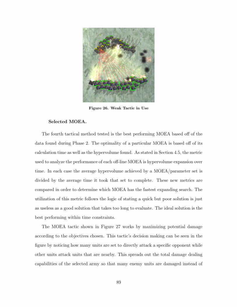
Figure 26. Weak Tactic in Use
Selected MOEA.
The fourth tactical method tested is the best performing MOEA based off of the
data found during Phase 2. The optimality of a particular MOEA is based off of its
calculation time as well as the hypervolume found. As stated in Section 4.5, the metric
used to analyze the performance of each off-line MOEA is hypervolume expansion over
time. In each case the average hypervolume achieved by a MOEA/parameter set is
divided by the average time it took that set to complete. These new metrics are
compared in order to determine which MOEA has the fastest expanding search. The
utilization of this metric follows the logic of stating a quick but poor solution is just
as useless as a good solution that takes too long to evaluate. The ideal solution is the
best performing within time constraints.
The MOEA tactic shown in Figure 27 works by maximizing potential damage
according to the objectives chosen. This tactic’s decision making can be seen in the
figure by noticing how many units are set to directly attack a specific opponent while
other units attack units that are nearby. This spreads out the total damage dealing
capabilities of the selected army so that many enemy units are damaged instead of
89

Figure 27. MOEA Tactic in Use
focusing completely on a single target. The selected units who are attacking enemies
near to the main enemy target are expecting to deal a certain amount of area of effect
damage which kills the primary target through indirect fire.
Online Simulation Measurement Metrics.
The metrics used for measuring and comparing Phase 3 are based on the speed
and efficiency of gameplay. The objective of the tactics algorithm is not just to win,
but to win effectively. The efficiency of the win can be based on the following factors:
Win/Loss Ratio.
The most important aspect of measuring the efficiency of a win is first to actually
win. The first metric measured in Phase 3 is the Win/Loss ratio between each of the
potential tactics options. This metric is binary - if an agent wins a specific match it
is given a 1, otherwise it is given a 0. The total result provides an average win rate
against opposing tactics options which are derived by summing the total outcomes of
an agent and dividing by the total number of runs.
90

Time of Battle.
Another objective of an agent is to win as quickly as possible in order to free up
an army for other use. If an army is kept in one place for too long then it cannot be
used as reinforcements or it could allow the opposing player to fortify their base in
expectation of the upcoming attack. For this reason the time of battle is an important
metric to track. The start time of battle is when the two armies are aware of each
other and the simple movement command becomes an attack command. This can
be tracked in game by watching the movement marker for each unit in an army. A
green marker means that a unit is passively moving towards a destination. A red
line shows that a unit is engaging a target. Combat start time is when the first red
targeting line appears in a simulation. Combat ends when one side’s forces have been
completely eliminated.
Remaining Units.
Another important consideration in battle is to minimize the number of losses
suffered during a conflict. This metric measures the number of units remaining at the
end of battle, and uses it to determine the effectiveness of a specific tactic. A tactic
that wins with an 80% success rate but with high losses may not be as useful as a
tactic with a 70% success rate with low losses.
Average Remaining Health of Units.
The final objective builds off of the concept built with the Remaining Units metric.
The summation of the remaining HP of all units is taken and then divided among
the number of remaining units. The purpose behind this objective is to gauge the
usefulness of the remaining units. An army of numerous heavily damaged units are
not as useful in later conflicts as a smaller army of stronger units. This metric is used
91

to gauge how a tactic performs against others and how that tactic acts to preserve
its units in battle.
4.7 Chapter Summary
This chapter provides a more in-depth review of the design process used to perform
the experimentation testing the viability of MOEA controlled RTS AI agents with
regard to the RTS tactical decision making problem. This chapter continues from the
initial framework discussed in Chapter 3, and provides additional information on the
specific layout and function of each part of the experiment. The processes described
in this chapter lead to the acquisition of the data in Appendices B, C, and C, which
are then used to perform the analysis in Chapter 5.
92

V. Results and Analysis
5.1 Introduction
This describes the results achieved by completing the processes defined in Chapter
IV: Design of Experiments. It also provides analysis of these results to determine the
links behind decisions made in the experimental design and the overall outcome. The
analysis begins with the evaluation of the integration of the PyGMO MOEA code
with the Spring RTS Engine. Once the initial integration has been completed, an
offline simulator is used to test the capabilities of three different MOEAs: NSGA-II,
SPEA2, and NSPSO. These three MOEAs are tested under different generational
limits and population sizes in order to determine the effects of modifying their base
parameters. Once the best MOEA has been found via offline testing, the AFIT agent’s
tactical control manager is modified in order to use the best performing MOEA as an
online tactical decision making tool. This tactical tool is then tested against various
scripted tactics in order to evaluate the MOEA’s online performance.
5.2 Design Phase 1 - Integrating Spring and PyGMO
The first phase of this experimental design is the mapping of combat between
two armies composed of 25 tanks each into a grid layout, and the conversion of that
grid into an array usable within the PyGMO code. The first analysis of the default
attack formation for this layout is performed by creating 25 stumpy tanks in game,
and watching how they position to attack a specific point. The results for this test
are that the tanks line up in a roughly semi-circular shape and are 4-5 units deep at
the center point. A screenshot of the animation is shown shown in figure 28.
Once this initial test is complete, the next step is to ensure that in an actual battle,
the tanks are given enough time to position themselves in the same manner they use
93

Figure 28. Simulation of 25 Tanks Attacking a Single Point
Figure 29. Two Examples of 25 vs 25 Tank Battles
94
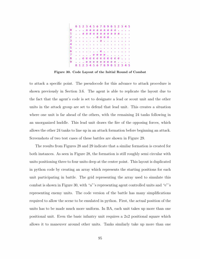
Figure 30. Code Layout of the Initial Round of Combat
to attack a specific point. The pseudocode for this advance to attack procedure is
shown previously in Section 3.6. The agent is able to replicate the layout due to
the fact that the agent’s code is set to designate a lead or scout unit and the other
units in the attack group are set to defend that lead unit. This creates a situation
where one unit is far ahead of the others, with the remaining 24 tanks following in
an unorganized huddle. This lead unit draws the fire of the opposing forces, which
allows the other 24 tanks to line up in an attack formation before beginning an attack.
Screenshots of two test cases of these battles are shown in Figure 29.
The results from Figures 28 and 29 indicate that a similar formation is created for
both instances. As seen in Figure 28, the formation is still roughly semi circular with
units positioning three to four units deep at the center point. This layout is duplicated
in python code by creating an array which represents the starting positions for each
unit participating in battle. The grid representing the array used to simulate this
combat is shown in Figure 30, with “a”’s representing agent controlled units and “e”’s
representing enemy units. The code version of the battle has many simplifications
required to allow the scene to be emulated in python. First, the actual position of the
units has to be made much more uniform. In BA, each unit takes up more than one
positional unit. Even the basic infantry unit requires a 2x2 positional square which
allows it to maneuver around other units. Tanks similarly take up more than one
95

block due to their size. Limiting tanks to taking up a 1x1 square allows them to be
positioned in such a simply designed array. The actual locations of each unit is also
restricted to directly match Figure 30. This is done to create a uniform “first round of
combat” that can be used to compare MOEA performance. Online testing will allow
positions to be updated in real time. Another simplification required for the array
construction is ignoring tank and turret direction. In the Spring RTS engine, units
are restricted to only firing in the direction they are facing. Stumpy tanks, and other
turreted units have an independently controlled turret that can turn faster than the
main body, but this aiming still requires time that is not accounted for in the python
representation of combat.
Once the units are placed and x and y coordinates are assigned to each, the next
step is to apply the other attributes that define a stumpy tank. The actual hit point
scores of the units are able to be maintained - each unit has 1530 hit points. The
damage can also be carried directly over from the balanced annihilation mod info page
[63]. Stumpy units do 97 damage per direct damage hit, and 48 damage via indirect
fire. The range for this indirect damage is modified to only apply to adjacent targets.
For example if the enemy unit at position (7,6) is hit, then the units at (6,7), (7,7),
and (8,7) take a fraction of the primary weapon damage as indirect splash damage.
The extent of this indirect damage is modified by the proximity of adjacent units to
the primary target. Due to the simplification of the map to a simple grid pattern,
the distance for each of these adjacent units are the same.
Once the model has been constructed in can be used to begin Phase 2 testing.
Phase 2 testing uses the three different MOEAs to be compared and determines how
well they perform in the RTS tactical decision making problem.
96

5.3 Testing of Phase 2 - Offline Simulation
Phase 2 testing begins with running the code generated in Phase 1 against various
MOEAs with different parameters. As stated in Section 3.5, the MOEAs under test
are SPEA2, NSGA-II, and NSPSO. The parameters tested are population capacity
and generation limit. Population sizes used are 20, 40, 60, 80, and 100. Generational
limits are 2, 3, 4, and 5. Each combination of generation limit and population size
are tested 10 times. The analysis of the performance of each MOEA over the given
problem domain are discussed in the following subsections.
Analysis of MOEA Performance in Tactics Optimization.
This section provides the data and analysis for phase 2 testing. This data includes
a compilation of average data values with regards to the metrics used to analyze
MOEA performance with regards to parameter changes and MOEA performance.
This raw data is then used to build a series of box plots which visually represent the
performance of MOEA parameter combinations. The raw data used to create both the
tables and the box plots can be found in Appendix B. The analysis of each population
of solutions is performed by measuring the hypervolume of the pareto front generated
by each individual population. The solutions contained in each population each build
a separate Pareto front which represents the effectiveness of that population. Each
member of the population represents a single point in four dimensional space, due to
the use of four different objective values. The volume of the four dimensional space
bounded by all members of the population can then be used as a metric to judge the
optimality and performance of one MOEA combination over another, as more ideal
solution sets are closer to the “true” Pareto front and farther away from the point of
measure.
97
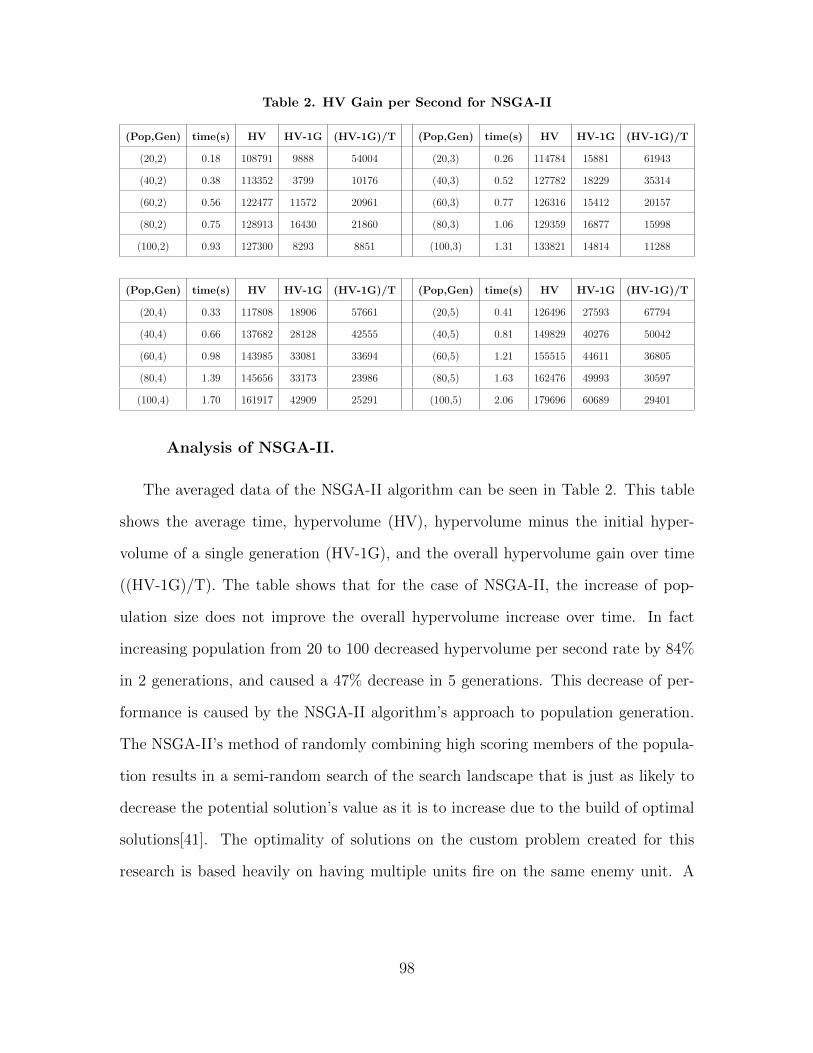
Table 2. HV Gain per Second for NSGA-II
(Pop,Gen) time(s) HV HV-1G (HV-1G)/T (Pop,Gen) time(s) HV HV-1G (HV-1G)/T
(20,2) 0.18 108791 9888 54004 (20,3) 0.26 114784 15881 61943
(40,2) 0.38 113352 3799 10176 (40,3) 0.52 127782 18229 35314
(60,2) 0.56 122477 11572 20961 (60,3) 0.77 126316 15412 20157
(80,2) 0.75 128913 16430 21860 (80,3) 1.06 129359 16877 15998
(100,2) 0.93 127300 8293 8851 (100,3) 1.31 133821 14814 11288
(Pop,Gen) time(s) HV HV-1G (HV-1G)/T (Pop,Gen) time(s) HV HV-1G (HV-1G)/T
(20,4) 0.33 117808 18906 57661 (20,5) 0.41 126496 27593 67794
(40,4) 0.66 137682 28128 42555 (40,5) 0.81 149829 40276 50042
(60,4) 0.98 143985 33081 33694 (60,5) 1.21 155515 44611 36805
(80,4) 1.39 145656 33173 23986 (80,5) 1.63 162476 49993 30597
(100,4) 1.70 161917 42909 25291 (100,5) 2.06 179696 60689 29401
Analysis of NSGA-II.
The averaged data of the NSGA-II algorithm can be seen in Table 2. This table
shows the average time, hypervolume (HV), hypervolume minus the initial hyper-
volume of a single generation (HV-1G), and the overall hypervolume gain over time
((HV-1G)/T). The table shows that for the case of NSGA-II, the increase of pop-
ulation size does not improve the overall hypervolume increase over time. In fact
increasing population from 20 to 100 decreased hypervolume per second rate by 84%
in 2 generations, and caused a 47% decrease in 5 generations. This decrease of per-
formance is caused by the NSGA-II algorithm’s approach to population generation.
The NSGA-II’s method of randomly combining high scoring members of the popula-
tion results in a semi-random search of the search landscape that is just as likely to
decrease the potential solution’s value as it is to increase due to the build of optimal
solutions[41]. The optimality of solutions on the custom problem created for this
research is based heavily on having multiple units fire on the same enemy unit. A
98

random search has no way to generate solutions that focus fire on enemies, and these
solutions are necessary to create good objective scores.
Figure 31. Box Plots for HV Increase Over Time for NSGA-II 20 Population
The NSGA-II performed best with a population of 20. The statistical analysis for
this evaluation is shown in Figure 31. This box plot shows that over the course of five
generations the NSGA-II algorithm maintains a high level of variance, while showing
only a slight increase in effectiveness. The mean value throughout each generation
stays between a score of 50,000 and 75,000. The other population tests, shown in
Figure 32 show even worse results, with the majority failing to obtain a score of
50,000.
Analysis of SPEA2.
The results of the SPEA2 algorithm are shown in Table 3. The SPEA2 algorithm
performed 17% to 35% faster than the NSGA-II algorithm, but it is not able to
consistently outperform on a hypervolume per second basis, as shown in Figures
33 and 34. For the combination of 20 population and 3 generations, the NSGA-II
99

Figure 32. Box Plots Showing HV Increase Over Time for NSGA-II Algorithm
Table 3. HV Gain per Second for SPEA2
(Pop,Gen) time(s) HV HV-1G (HV-1G)/T (Pop,Gen) time(s) HV HV-1G (HV-1G)/T
(20,2) 0.15 110446 4732 32081 (20,3) 0.18 111660 5946 32046
(40,2) 0.30 113061 415 1384 (40,3) 0.37 120926 8280 22073
(60,2) 0.46 123641 14283 30907 (60,3) 0.58 125101 15742 26971
(80,2) 0.62 120785 6007 9647 (80,3) 0.79 132537 17759 22342
(100,2) 0.77 120852 2033 2626 (100,3) 0.96 139219 20400 21176
(Pop,Gen) time(s) HV HV-1G (HV-1G)/T (Pop,Gen) time(s) HV HV-1G (HV-1G)/T
(20,4) 0.22 120426 14712 65799 (20,5) 0.26 131388 25673 100252
(40,4) 0.45 141023 28378 62851 (40,5) 0.54 154609 41963 78146
(60,4) 0.69 146389 37030 53962 (60,5) 0.81 172041 62682 77386
(80,4) 0.94 152152 37374 39801 (80,5) 1.08 162475 47697 44082
(100,4) 1.19 156868 38049 32086 (100,5) 1.40 180566 61746 44215
100

Figure 33. Box Plots for HV Increase Over Time for SPEA2 20 Population
algorithm doubled the SPEA2’s score, but on the 100 population and 3 generation
test SPEA2 outmatched NSGA-II. This lack of consistency is caused by the SPEA2’s
search process. The SPEA2 forces a certain degree of separation between each solution
on the Pareto front, which could remove a potentially better solution from being used
in the next generation [43]. This forced widening of the search area via Pareto front
manipulation prevents the SPEA2 from providing consistent results.
The 20 population SPEA2 experiments performed the best according to statistical
analysis, as shown in Figure 33. While the algorithm has a slow start in comparison
to NSGA-II, with a score of less than 50,000, at 5 generations the algorithm is able
to reach an average score of 100,000. This score is achieved with a higher degree,
of variance, however, as shown by the increased scaling of the Y axis. The other
population options for the SPEA2 algorithm which are shown in Figure 34 show that
the SPEA2 algorithm’s performance follows the same track as NSGA-II. Increased
population size does not have a positive effect on the rate of hypervolume expansion.
101

Figure 34. Box Plots Showing HV Increase Over Time for SPEA2 Algorithm
Table 4. HV Gain per Second for NSPSO
(Pop,Gen) time(s) HV HV-1G (HV-1G)/T (Pop,Gen) time(s) HV HV-1G (HV-1G)/T
(20,2) 0.15 133039 23486 156573 (20,3) 0.19 161719 52165 276901
(40,2) 0.30 146446 29968 99892 (40,3) 0.38 193610 77132 203603
(60,2) 0.46 150673 26351 57098 (60,3) 0.57 251850 127528 223943
(80,2) 0.62 155263 31266 50365 (80,3) 0.77 225272 101276 132153
(100,2) 0.79 166060 42336 53845 (100,3) 0.97 313424 189700 194767
(Pop,Gen) time(s) HV HV-1G (HV-1G)/T (Pop,Gen) time(s) HV HV-1G (HV-1G)/T
(20,4) 0.23 207710 98156 437031 (20,5) 0.26 257180 147626 567792
(40,4) 0.45 271242 154764 343238 (40,5) 0.52 398017 281539 539559
(60,4) 0.69 313963 189641 276168 (60,5) 0.80 525404 401082 498732
(80,4) 0.93 345348 221352 238989 (80,5) 1.10 447954 323957 296122
(100,4) 1.17 512206 388482 332127 (100,5) 1.37 577163 453440 330037
102

Figure 35. Box Plots for HV Increase Over Time for NSPSO 20 Population
Analysis of NSPSO.
The NSPSO algorithm performed the best out of the three tested MOEAs, the
average results of which are shown in Table 4. The NSPSO algorithm completes its
search faster than both the NSGA-II and SPEA2 algorithms, and is also able to cover
the most hypervolume during its search. This leads the NSPSO algorithm to obtain
to a much higher hypervolume per second increase than the other two MOEAs.
The top performing combination of NSPSO parameters is 20 population mem-
bers with 5 generational evolutions. This result matches with the best performing
parameter sets of NSGA-II and SPEA2, although the NSPSO algorithm’s output is
much better than either of the other two tested MOEAs. While the NSPSO algo-
rithm shows a lot of variance in Figure 35, the worst population member found is
equivalent or better than the best members found in either NSGA-II or SPEA2. The
best performing member within the NSPSO population set for 20 population and 5
generations almost reaches a score of 2 million. This difference in performance be-
103

Figure 36. Box Plots Showing HV Increase Over Time for NSPSO Algorithm
tween MOEAs clearly shows that the NSPSO algorithm outperforms the alternatives
with regards to the RTS tactical decision making problem.
While the best selection of parameters for the NSPSO algorithm shows a 500%
improvement over alternatives, the remainder of parameter settings in Figure 36 show
that experiments with higher population also outperform any results from NSGA-II
or SPEA2. These results also show a faster slope increase over the course of more
generations, showing that the NSPSO algorithm is capable of continuing to improve.
The high level of performance generated by the NSPSO algorithm is made possible
by the overall search landscape for the tactical decision making problem. In this
problem a certain number of units are required to fire on an enemy in order to
destroy it. The NSPSO is able to create a random initial population, and have the
other 19 members of the population slowly migrate towards the best solution. This
ensures that the best member of the population is maintained while other members
104

of the population search the nearby area for the “peak”, or where the exact number
of friendly tanks fire on a single enemy in order to destroy it. This ability shows that
the 20 population - 5 generation search using NSPSO is the best performing option
out of all MOEAs that are tested.
Conclusions of Offline Simulation.
The offline testing of the three MOEAs: NSGA-II, SPEA2, and NSPSO ended in
a clear differentiation between the performances of each option. NSGA-II required
the longest amount of time to calculate and had a wide margin in resulting cham-
pion solution values. This poor performance is based on the mechanics behind the
NSGA-II algorithm itself and shows how a random selection of population members
and combination is not suitable for the tactical decision making problem at hand.
The SPEA2 algorithm, while fast, is not able to achieve consistent high quality
results through testing. The SPEA2 algorithm’s requirement of forcing a maximum
amount of space between members of a population is a detriment when attempting to
analyze the given search landscape. In the tactical decision making search landscape a
“more optimal” solution is most likely next to the currently most optimal population
member. This “more optimal” solution can typically be achieved by modifying the
current best solution to have a few more units focus on the primary target in order
to destroy that target this round. By forcing individuals to be a certain degree apart
the SPEA2 search prevents these potentially useful neighbors from being explored,
which results in a lower quality solution than what other MOEAs can find. In the
search landscape of the tactical decision making problem, the entirety of the SPEA2
algorithm’s search methodology works against it when it comes to finding solutions.
The NSPSO algorithm is the most optimal solution found through this series of
experiments. NSPSO achieves the best solutions in the fastest amount of time due
105

to the process that it uses to create the next generation. This constant moving
of the population members towards the currently “most optimal” member provides
extensive coverage of a very localized portion of the search landscape which means
that an in-depth analysis of a small set of solutions is performed. This in-depth
analysis of a small area works very well with the focus fire objective used in the
PyGMO problem, which is why the NSPSO MOEA is capable of easily reaching six
figure hypervolume per second rates while NSGA-II and SPEA2 struggle to break
100,000. This focused search provides very good solutions with small populations,
and the addition of population members does not seem to be worth the additional
computational time required.
The most optimal setup found through this series of tests is to use the NSPSO
algorithm with 20 population and a 5 generation limit. This option is able to achieve
an average of the top rate of hypervolume increase per second within a quarter of
a second. The NSPSO algorithm appeared to perform at a similar rate with a 40
population and a 5 generation limit, however this doubled the required calculation
time. The 20 population option is chosen in order to allow the AFIT AI agent to
more quickly respond to battlefield changes and minimize the amount of computation
required to adapt to new situations.
5.4 Phase 3 - Online Simulation
This section describes the overall results of the on-line simulation between the
four tested tactic methods. The comparative results can be seen in the bar graphs
found in Figures 37, 38, 40, and 42. For these graphics, each tested tactic has its own
color, and data related to that tactic is only used if that tactic won. For example, the
“weak” tactic did not receive any victories in 20 attempts when facing “MOEA” and
“proximity”, so very little green shows in any of the graphics. Each of these matchups
106

Table 5. Results of Default Tactic VS Other Tactics
Default VS: Win Rate Time Units Average HP
Proximity 60% 0:43 6.42 940.89
Weak 90% 0:37 6.72 1265.6
MOEA 20% 0:35 10 827.13
are performed twenty times, with each army starting at the top of the screen ten times
and at the bottom of the screen ten times.
Analysis of the Default Tactic.
The results of the default tactic can be found in Table 5. This table only includes
data from when the default tactic won its matchup. The default tactic achieves an
overwhelming 90% win rate against the weak tactic, and a 60% win rate against the
proximity tactic. This tactic did not perform well against the MOEA tactic, as it
achieved only a 20% win rate. The default tactic’s method of having the entire group
focus fire on the closest enemy unit results in additional area of effect damage to
nearby enemy units. This focused damage not only quickly destroys the unit, but
it also causes the outgoing fire to sweep across the enemies as they approach which
results in very little wasted fire. This is an advantageous method to use when fighting
in a confined area, but loses a lot of potential if they enemy is spread out since there
is less area of effect damage and more wasted shots.
Analysis of the Proximity Tactic.
The proximity tactic operates by ordering each individual unit to attack the closest
enemy relative to that unit’s position. The results of this tactic can be found in
Figure 6. This tactic causes the group to fire on a few enemy units at a time, which
107

Table 6. Results of Proximity Tactic VS Other Tactics
Proximity VS: Win Rate Time Units Average HP
Default 40% 0:39 5.87 1017.65
Weak 100% 0:42 8.42 1229.54
MOEA 30% 0:42 6.83 736.43
Table 7. Results of Weak Tactic VS Other Tactics
Weak VS: Win Rate Time Units Average HP
Default 10% 0:42 7 1106.29
Proximity 0% N/A N/A N/A
MOEA 0% N/A N/A N/A
is detrimental in the short term, but helps in a longer battle. This is because a
more focused fire in the beginning stages of a battle destroys enemy units faster,
which significantly reduces the amount of incoming damage. Spreading out targets
slows down the rate of the initial kills. Conversely during the last stages of a fight
enemies are all typically damaged to some degree. Spreading out fire on different
targets minimizes the damage wasted at this point in the battle, and helps destroy
the remaining enemies.
Analysis of the Weak Tactic.
The weak tactic operates by constantly targeting the enemy with the lowest re-
maining HP. This results in a random initial target, followed by a sweeping motion
across the battlefield. After the first enemy is destroyed, nearby enemies have been
weakened by the area of effect damage. The weakest of these damaged units is se-
108
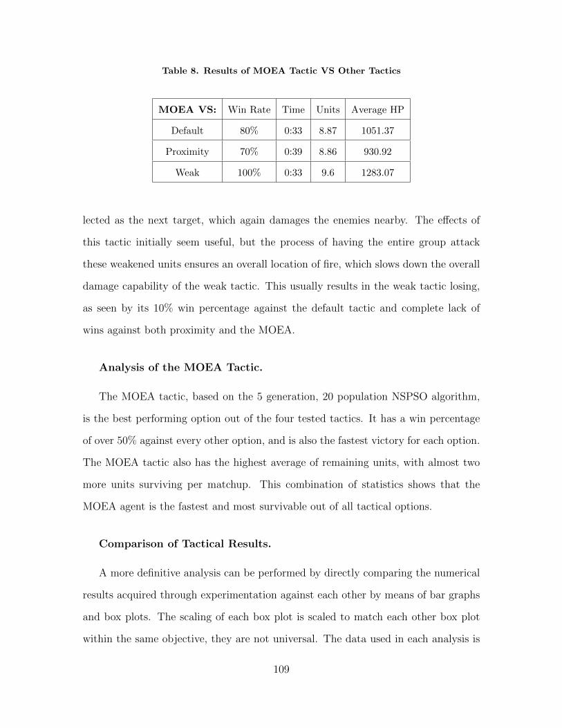
Table 8. Results of MOEA Tactic VS Other Tactics
MOEA VS: Win Rate Time Units Average HP
Default 80% 0:33 8.87 1051.37
Proximity 70% 0:39 8.86 930.92
Weak 100% 0:33 9.6 1283.07
lected as the next target, which again damages the enemies nearby. The effects of
this tactic initially seem useful, but the process of having the entire group attack
these weakened units ensures an overall location of fire, which slows down the overall
damage capability of the weak tactic. This usually results in the weak tactic losing,
as seen by its 10% win percentage against the default tactic and complete lack of
wins against both proximity and the MOEA.
Analysis of the MOEA Tactic.
The MOEA tactic, based on the 5 generation, 20 population NSPSO algorithm,
is the best performing option out of the four tested tactics. It has a win percentage
of over 50% against every other option, and is also the fastest victory for each option.
The MOEA tactic also has the highest average of remaining units, with almost two
more units surviving per matchup. This combination of statistics shows that the
MOEA agent is the fastest and most survivable out of all tactical options.
Comparison of Tactical Results.
A more definitive analysis can be performed by directly comparing the numerical
results acquired through experimentation against each other by means of bar graphs
and box plots. The scaling of each box plot is scaled to match each other box plot
within the same objective, they are not universal. The data used in each analysis is
109

Figure 37. Comparison of Win Percentages Between Tactic Options
only allowable when a particular tactical method wins. The Weak tactic, having only
two successes throughout all experimental runs, has its data based on two distinct
data points. The remainder of the data is compiled in a similar method.
Win Rate.
Figure 37 shows that the MOEA tactic (shown in purple) is capable of matching
or outperforming alternatives against each opponent. The MOEA tactic has an 80%
win rate against the default tactic vs. the proximity tactic’s 40%. The MOEA tactic
also outperforms the default tactic when facing the proximity tactic by maintaining a
10% higher rate of success. Both the MOEA and the Proximity tactic achieve a 100%
win rate against the group attack weakest tactic. The data shows that the Default
tactic has a slight advantage over the Proximity tactic. The Proximity tactic has a
slight advantage over the otehr scripted methods when attacking the Weak tactic.
The MOEA based tactic outperforms all scripted alternatives against all opponents.
110

Figure 38. Comparison of Battle Duration Between Tactic Options
Battle Time.
Battle time is used as an objective in order to determine how long an army is held
up by an opposing army. The best performing decisions complete the battle quickly
and successfully in order to allow remaining forces to be used in other areas as soon
as possible. Figure 38 shows that the MOEA tactic, shown in purple, is capable of
completing combat faster on average than all alternatives in against every opponent.
The average data from Figure 38 is expanded on by the statistical information in
Figure 39, which shows a very similar statistical range for each opponent. The largest
variation of battle times occur when the Default tactic and the MOEA tactic face
against the Proximity tactic. This similarity shows that there may be some instances
where the Default tactic’s method of attacking the closest enemy may be faster than
attempting to spread fire against all opponents. The data for each tactic facing the
Weak tactic shows a very small variance, which means that each method consistently
achieves the same results through experimentation.
111

Figure 39. Box Plots For Online Battle Duration
Figure 40. Comparison of Units Remaining After Battle Between Tactic Options
112

Figure 41. Box Plots For Number of Units Remaining
Remaining Units.
Another important metric of grading the optimality of a battle’s outcome is to
measure the number of units remaining. While winning a battle is good, winning that
same battle with a larger number of forces remaining is better. 40 shows a comparative
bar graph between the online performance of each tested tactical decision making
method. As in the previous objectives, the MOEA tactic continues to outperform
every other tactic tested. Therefore current results show that the MOEA tactic has
the highest win rate, completes battles the fastest, and has the most units remaining
after combat on average.
The statistical analysis of each tactical method’s performance is shown in Figure
41. These box plots show that the MOEA tactic has a larger variance than the other
113

Figure 42. Comparison of Average Remaining HP After Battle Between Tactic Options
metrics when facing the Default Tactic or Proximity tactic, but it maintains a smaller
variance against the Weak tactic. It is also important to note that while the MOEA
tactic has a larger variance than alternatives, the mean of its variance is much higher
than Default or Proximity, which shows that the MOEA tactic has a high probability
of continuing to outperform any tested alternative.
Remaining Hit Points.
The final objective used to grade the performance of a winning battle is the average
remaining HP of all remaining units. This objective is used in order to determine the
future survivability of each remaining unit in future battles. The comparative results
of this objective can be seen in Figure 42. Unlike the previous objectives, the MOEA
tactic was not the best performing metric on average. However, the discrepancy
between the MOEA tactic’s performance and alternatives is much smaller than in
earlier metrics. Where previous differences were in the range of 15% to 20%, the
difference in the average HP remaining is less than 5%. This shows that the MOEA
tactic still performs well with regards to the other tested tactics.
114

Figure 43. Box Plots For Average HP Remaining
115

The statistical analysis of the various tactics’ performance with regards to remain-
ing HP values can be seen in Figure 43. The MOEA tactic has the highest variance
in the majority of battles, with only the Proximity vs Weak coming close to the range
of variance. These results show that remaining HP after combat is very difficult to
converge to an absolute expectation.
Conclusions of On-Line Battles.
The on-line simulation shows a clear distinction between the performance of the
various tactical options. The MOEA option is the clear winner, with the best results
in each of the obtained metric scores. The majority of the losses suffered by the
MOEA agent are caused by choosing an edge unit as the scout, which caused the
entire army to group against the side of the pathway. This bunching up prevented
many tanks from spreading out, which reduces outgoing fire and ensured that more
friendly units are hit by the enemy’s area of effect damage.
Another consideration in the performance of the battles is the speed at which
armies moved into position. Most armies are able to move relatively quickly, but the
MOEA tactic’s constant readjustment of targets during approach all but ensured that
its tanks would arrive and form up slower than the opponent. Also, the army located
on the lower section of the map appears to have a distinct advantage due to very
small details about the map’s design. The map has a slightly smaller area directly
above the standard battlefield, which means the upper army is more constrained in
how they move which sometimes leads to reduced effectiveness in combat.
5.5 Comparison of Results to Previous Research
While not directly comparable to the research performed in the RTS tactical
decision making world due to the difference in approaching the base problem, some
116

preliminary comparisons can be made based off of the effective methods results. In
Churchill’s paper utilizing a modified Alpha-Beta script considering durations [13],
he is able to achieve a 91% to 92% win rate against scripted opponents within 5 ms.
The MOEA agent is not capable of reaching the same level of performance, but is also
analyzing a much larger battlefield. Churchill’s work focuses on placing a variety of 8
vs 8 armies against each other. The MOEA analysis is based off of a 25 vs 25 single
unit battle. While MOEA performance is much slower than the 5 ms restriction used
in Churchill’s paper, it is still capable of actively changing actions based on battlefield
situations. His process is expanded to create a portfolio greedy search algorithm for
analysis of larger scale combat [34]. This modified search was only tested against
other alpha-beta searches in order to present a comparative level of improvement
over his previous developments.
Additional research has been performed in the past analyzing the use of Monte
Carlo Tree Search methods on the RTS tactical decision making problem [64]. In his
research, Balla utilizes the UCT algorithm in order to train an agent to make combat
decisions in the Wargus RTS environment. His research shows that while MCTS are
trainable to achieve objective optimization, the UCT algorithm was unable to achieve
online performance, even with small army sizes of 4 units. This outcome shows that
the initial results of MOEAs for use in solving the RTS tactical decision making
problem are promising, as they allow solutions to be generated online without any
prior training.
5.6 Chapter Summary
This chapter reviewed and analyzed the data found during the experimentation
into the use of a MOEA as a tactical decision making tool in RTS games. A custom
problem representing the RTS tactical decision making problem is developed and in-
117

tegrated into the PyGMO code. This code is then added to the Spring RTS engine
for use in online simulations. The three MOEAs under test are executed in the simu-
lated first round of combat, with the NSPSO algorithm drastically outperforming the
alternatives due to its more focused search methods. Finally, the NSPSO algorithm
is placed into the MOEA tactic for use in online testing. This MOEA tactic outper-
forms all three of the scripted methods, and demonstrates that MOEAs can be used
as tactical decision making tools in a real time environment.
118

VI. Conclusion
6.1 Evaluation of Results
The results of the series of experiments accomplishes the objectives stated in
Chapter 1.4. The data acquired validates that MOEAs can perform correctly and
efficiently as a tactical decision making tool in an RTS AI agent, and have potential
for use in actual military simulation hardware. The final results of performance anal-
ysis show that the MOEA based agent is capable of matching the expected win rate
of tactical decision making methods discussed in Chapter 2.7, achieving an 80% win
rate against the default tactic with requiring any sort of prior training or intensive
tree search analysis. While initial testing required offline comparison between differ-
ent MOEAs, once an MOEA is selected there is no longer a requirement for offline
standardization in order to allow that MOEA to perform in an online environment.
Each objective is satisfied, with objective one serving as a design requirement
for the successful testing of objectives two and three. Objective two is thoroughly
investigated and the results of the three tested MOEAs indicate that knowledge of the
expected structure of the fitness function results in a better selection of an MOEA for
use, as shown in Section 5.3. This difference of utility between MOEAs is explained by
the ”No Free Lunch” theorem (Section 2.9), which states that there is no such thing as
a universally optimal algorithm that can efficiently solve all problems. Each problem
has an optimal method of approach which outperforms other potential solutions, but
this method of approach does not perform optimally in other search landscapes [47].
Therefore the user must have an understanding of the search landscape in order to
choose the best MOEA option.
The aggregated fitness function of the RTS tactical decision making problem is
found to have numerous peaks within a small range of each other due to the heavy
119

reliance of a ”kill” during a round of combat. There are numerous ways to achieve a
”kill” within combat and that typically a solution with a high amount of focused fire
leads to a solution very close to one with a ”kill”. This analysis of the aggregated
fitness function for a tactical decision making agent performed for this series of ex-
periments is correct in stating that the NSPSO algorithm performs the ”best” due to
its ability to focus the search area of future generations around these semi-optimal
solutions. This more focused search of the landscape allows the particle swarm based
NSPSO algorithm to find results with nearly five times the hypervolume metric in-
crease per second of the population of solutions found by the more uniform search
structure used by SPEA or the random search method used by NSGA. Therefore
the result of objective two is that out of the three MOEAs chosen for this research,
NSPSO outperformed SPEA2 and NSGA-II by a large margin as shown in Section
5.3.
Objective three is performed by utilizing and analyzing the animations within the
Spring RTS engine. Each battle performed is viewed and measured in order to gather
the metrics used to measure the usefulness of the MOEAs and scripted tactics. By
using a series of online battles the NSPSO MOEA controlled tactical agent is placed
against a variety of scripted tactical methods. The MOEA outperformed the scripted
methods in all metrics considered. The MOEA tactic is able to combine a high
win rate and a fast battle completion time with a large amount of remaining units.
The use of multiple objectives when determining courses of action helps to overcome
some of the limitations created by the use of a single variable. For example, an
agent relying on a kill/death ratio or some modification thereof as it’s objective is
limited in capability when given an army that cannot outright kill an opponent in
a single round. The required foresight required to determine the course of future
120

actions requires more computational time which is not available to the AFIT tactical
decision manager in its current form.
The current version of the AFIT tactical decision manager requires a large amount
of processing power for the quarter second needed to generate a solution. This increase
in processing power results in noticeable lag to a human opponent, which in turn slows
down gameplay and human player interaction with the Spring Engine. The lag is more
pronounced during the initial phases of combat between the time when armies come
within visual range of each other and lasts until units move into position. Other
tactical AI agents are not affected by this slowdown of the game, as their commands
run within the game environment itself and are therefore not affected by the game
user interface lockdown caused by prolonged processing.
The overall goal for this research, stated in Chapter 1, is accomplished. An MOEA
has been successfully integrated within the existing AFIT agent, and supplies solu-
tions that are capable of beating many different scripted agents. The AFIT agent
is now able to defeat these scripted agents in battle without requiring previous ex-
perience against an opponent or off-line computation and training. Once engaged
in combat the agent is able to quickly redetermine optimal firing solutions within a
quarter of a second.
6.2 Future Work
There are various vectors future researchers can follow due to the scope of inte-
grating AI into RTS games:
• Optimize building locations to optimize economy generation and maintain open
pathways
• Integrate the capability to change strategies to counter opponents
121

• Integrate movement into the tactical decision making manager
• Reduce calculation time of the tactical manager to reduce lag impact to human
players
• Develop a new scouting manager which would remove the AFIT AI agent’s
reliance of removing fog of war
Each of these areas are important upgrades to the current performance of the
agent as well as another way to improve its ability to serve as a method to train
military personnel on battlefield decision making methods.
6.3 Final Remarks
The research presented in this thesis shows a strong argument for the integra-
tion of MOEAs into tactical decision making agents in both RTS and other military
combat simulations. The additional time required for the MOEA in comparison to
other scripted methods is negligible, and the results of the MOEA far exceed the
capabilities of the tested scripted agents, and performed as well as results achieved
in previous research [13, 37]. With more effort the time requirements for MOEA can
be further mitigated and additional command options can be included to create a
more robust agent capable of decision making in many different environments. The
integration of the MOEA controlled tactical decision manager significantly improves
the performance of the AFIT agent and serves as a stepping stone for future RTS AI
research.
122

Appendix A. Code for Offline Simulation
This Appendix provides the custom code created to integrate the PyGMO and
Spring RTS engine. The integration is performed through creating the moea.py file
and modifying the currently existing group.py manager in the AFIT agent.
1.1 moea.py
The moea.py file is a new manager placed in the .config/spring/AI/Skirmish/Tactics/*version*/python
folder. It is used to hold the custom MOEA problem class for the tactical decision
making problem as well as a new distance function to determine if enemies are within
range.
from PyGMO.problem import base
from math import *
from copy import deepcopy
import agent
def dist(p1,p2):
return((p1[0]-p2[0])**2 + (p1[1]-p2[1])**2)**0.5
class ROUND(base):
def __init__(self, allies=[[0,0,0,[0,0],0,0],[0,0,0,[0,0],0,0]],
↪→ enemies=[[0,0,0,[0,0],0,0],[0,0,0,[0,0],0,0]]):
# Solution is len(allies), with 4 objectives
self.allies = allies
self.enemies = enemies
super(ROUND,self).__init__(len(self.allies),0,4)
# Potential solutions are constrained to the number of enemies
123

self.set_bounds(0,len(self.enemies)-1)
def _objfun_impl(self,x):
# Matrices are [ID, HP, ALIVE, [XPOS,ZPOS], DAM, RANGE]
astart = self.allies
estart = self.enemies
anew = deepcopy(astart)
enew = deepcopy(estart)
# Simulate allied units firing
for i in range(0,len(anew)):
target = int(x[i])
if dist(anew[i][3],enew[target][3]) <= anew[i][5]:
enew[target][1] = enew[target][1] - anew[i][4]
# PROXIMITY DAMAGE CHECK
for k in range(0,len(enew)):
if k != int(x[i]):
if dist(enew[target][3],enew[k][3]) <= 48:
enew[k][1] = enew[k][1] - (anew[i][4]*(48 - dist(
↪→ enew[target][3],enew[k][3])) / 72)
# Check for destroyed enemy units
for i in range(0,len(enew)):
if enew[i][1] <= 0:
enew[i][1] = 0
enew[i][2] = 0
# Simulate enemies firing
124

for i in range (0,len(enew)):
pot_target = []
for j in range(0,len(anew)):
apos = anew[j][3]
epos = enew[i][3]
distance = dist(apos, epos)
pot_target.append(distance)
sort = sorted(range(len(pot_target)), key=pot_target.__getitem__
↪→ )
target = sort[0]
anew[target][1] = anew[target][1] - enew[i][4]
if anew[target][1] < 0:
anew[target][1] = 0
if anew[target][1] == 0:
anew[target][2] = 0
# Difference in number of units
f1 = 0
# Difference in HP totals
f2 = 0
# Difference in damage capability
f3 = 0
# Focus fire
f4 = 0
for i in range(0,len(enew)):
f1 = f1 + enew[i][2]
f2 = f2 + enew[i][1]
125

if enew[i][2] == 1:
f3 = f3 + enew[i][4]
for i in range(0,len(anew)):
f1 = f1 - anew[i][2]
f2 = f2 - anew[i][1]
if anew[i][2] == 1:
f3 = f3 - anew[i][4]
for i in range(0,len(enew)):
count = 1
for j in range(0,len(anew)):
if int(x[j]) == i:
f4 = f4 - count
count = count + 1
return (f1,f2,f3,f4,)
1.2 group.py
The group.py manager has been modified to implement the new PyGMO code.
Like the other python files it is also located in .config/spring/AI/Skirmish/*version*/python.
The changes made to account for a tactical decision making search include importing
moea.py at the beginning of the file and changing the attack function within the
manager. The original version of the attack function is saved as “default” and is used
as a comparison for test throughout Phase 3 of the experimentation.
import ctypes, math
import cdata
126

from PyGMO import *
from PyGMO.util import *
import moea
cdata.clb.move.argtypes = [ctypes.c_int, ctypes.c_int,
ctypes.c_float, ctypes.c_float]
class Group:
groupId = 0
def __init__(self, sid, gMap, unitManager, tactics):
self.sid = sid
self.gMap = gMap
self.unitManager = unitManager
self.units = []
self.defense = True # Am I the current defense group
self.order = ’move’
self.lastIdleEventFrame = 0
self.pendingIdleEvent = False
self.groupId = Group.groupId
self.mode = ’ground’
Group.groupId += 1
self.tactics = tactics
def remove(self, unit):
self.units.remove(unit)
if len(self.units) == 0:
127

return False
else:
return True
def add(self, unit):
if len(self.units) == 0:
if unit.defi.name in self.unitManager.aircraftNames:
self.mode = ’air’
else:
self.mode = ’ground’
self.units.append(unit)
unit.group = self
def setAttacking(self):
self.defense = False
self.units.sort(key=lambda unit: unit.defi.speed)
# Attack command modified 0.4.1
def attack(self):
if self.tactics == ’default’:
# Update gMap unit pos and time stamp
# clear old enemy values in gMap
for cell in self.gMap.iterateCells():
cell.enemyGroundUnits = []
# Get position of each enemy ground unit; enemyGroundUnits is a
↪→ dict
enemyMap = self.unitManager.enemyGroundUnits
size = len(enemyMap)
128

unitIds = enemyMap.keys()
enemyPositions = cdata.clb.getPositions(self.sid, unitIds, size)
for i in range(size):
enemy = enemyMap[unitIds[i]]
# attach pos to enemy unit
pos = enemyPositions[i]
enemy.pos = pos
# get cell containing pos
cell = self.gMap.getCellContainingPoint(pos)
# attach enemy unit to cell.enemy*.append(unit)
cell.enemyGroundUnits.append(enemy)
xavg, zavg = self._getCenterOfMass()
enemy = None
for cell in self.gMap.generateCells((xavg, 25.0, zavg)):
enemyBuilding = cell.enemyBuilding
enemies = cell.enemyGroundUnits
if not enemyBuilding is None:
# attack building
enemy = enemyBuilding
break
elif len(enemies) > 0:
# attack unit
enemy = self._getClosestEnemy(xavg, zavg, enemies)
break
if self.mode == ’air’:
enemy = self.unitManager.enemyCom
if enemy is None:
return
129

elif self.unitManager.LOS[enemy.unitId]:
self.order = ’attack’
self.attackEnemy(enemy)
else:
# Since enemy is outside of LOS, find a point to move to
self.order = ’move’
pos = enemy.pos
self.movePos = pos
if self.mode == ’air’:
for unit in self.units:
cdata.clb.move(self.sid, unit.unitId, pos[0], pos[2])
else:
target, guards = self.units[0], self.units[1:]
cdata.clb.move(self.sid, target.unitId, pos[0], pos[2])
self._guard(target, guards)
elif self.tactics == ’proximity’:
# Update gMap unit pos and time stamp
# clear old enemy values in gMap
for cell in self.gMap.iterateCells():
cell.enemyGroundUnits = []
# Get position of each enemy ground unit; enemyGroundUnits is a
↪→ dict
enemyMap = self.unitManager.enemyGroundUnits
size = len(enemyMap)
unitIds = enemyMap.keys()
enemyPositions = cdata.clb.getPositions(self.sid, unitIds, size)
for i in range(size):
enemy = enemyMap[unitIds[i]]
130

# attach pos to enemy unit
pos = enemyPositions[i]
enemy.pos = pos
# get cell containing pos
cell = self.gMap.getCellContainingPoint(pos)
# attach enemy unit to cell.enemy*.append(unit)
cell.enemyGroundUnits.append(enemy)
xavg, zavg = self._getCenterOfMass()
enemy = None
for cell in self.gMap.generateCells((xavg, 25.0, zavg)):
enemyBuilding = cell.enemyBuilding
enemies = cell.enemyGroundUnits
if not enemyBuilding is None:
# attack building
enemy = enemyBuilding
break
elif len(enemies) > 0:
# attack unit
enemy = self._getClosestEnemy(xavg, zavg, enemies)
break
if self.mode == ’air’:
enemy = self.unitManager.enemyCom
if enemy is None:
return
elif self.unitManager.LOS[enemy.unitId]:
self.order = ’attack’
for unit in self.units:
131

selfPos = cdata.clb.getUnitPosition(self.sid, unit.unitId
↪→ )
pot_target = []
for enemy in self.unitManager.enemyGroundUnits:
enemyPos = cdata.clb.getUnitPosition(self.sid, enemy)
Pos1 = [selfPos[0],selfPos[2]]
Pos2 = [enemyPos[0],enemyPos[2]]
distance = moea.dist(Pos1,Pos2)
pot_target.append([distance,enemy])
target = sorted(pot_target)
cdata.clb.attack(self.sid, unit.unitId, target[0][1])
else:
# Since enemy is outside of LOS, find a point to move to
self.order = ’move’
pos = enemy.pos
self.movePos = pos
if self.mode == ’air’:
for unit in self.units:
cdata.clb.move(self.sid, unit.unitId, pos[0], pos[2])
else:
target, guards = self.units[0], self.units[1:]
cdata.clb.move(self.sid, target.unitId, pos[0], pos[2])
self._guard(target, guards)
# ATTACK WEAKEST
elif self.tactics == ’weak’:
# Update gMap unit pos and time stamp
# clear old enemy values in gMap
for cell in self.gMap.iterateCells():
132

cell.enemyGroundUnits = []
# Get position of each enemy ground unit; enemyGroundUnits is a
↪→ dict
enemyMap = self.unitManager.enemyGroundUnits
size = len(enemyMap)
unitIds = enemyMap.keys()
enemyPositions = cdata.clb.getPositions(self.sid, unitIds, size)
for i in range(size):
enemy = enemyMap[unitIds[i]]
# attach pos to enemy unit
pos = enemyPositions[i]
enemy.pos = pos
# get cell containing pos
cell = self.gMap.getCellContainingPoint(pos)
# attach enemy unit to cell.enemy*.append(unit)
cell.enemyGroundUnits.append(enemy)
xavg, zavg = self._getCenterOfMass()
enemy = None
for cell in self.gMap.generateCells((xavg, 25.0, zavg)):
enemyBuilding = cell.enemyBuilding
enemies = cell.enemyGroundUnits
if not enemyBuilding is None:
# attack building
enemy = enemyBuilding
break
elif len(enemies) > 0:
# attack unit
enemy = self._getClosestEnemy(xavg, zavg, enemies)
133

break
if self.mode == ’air’:
enemy = self.unitManager.enemyCom
if enemy is None:
return
elif self.unitManager.LOS[enemy.unitId]:
self.order = ’attack’
pot_target = []
for enemy in self.unitManager.enemyGroundUnits:
enemyHP = cdata.clb.getUnitHealth(self.sid, enemy)
pot_target.append([enemyHP,enemy])
target = sorted(pot_target)
for unit in self.units:
cdata.clb.attack(self.sid, unit.unitId, target[0][1])
else:
# Since enemy is outside of LOS, find a point to move to
self.order = ’move’
pos = enemy.pos
self.movePos = pos
if self.mode == ’air’:
for unit in self.units:
cdata.clb.move(self.sid, unit.unitId, pos[0], pos[2])
else:
target, guards = self.units[0], self.units[1:]
cdata.clb.move(self.sid, target.unitId, pos[0], pos[2])
self._guard(target, guards)
# USE MOEA
elif self.tactics == ’moea’:
134

# Update gMap unit pos and time stamp
# clear old enemy values in gMap
for cell in self.gMap.iterateCells():
cell.enemyGroundUnits = []
# Get position of each enemy ground unit; enemyGroundUnits is a
↪→ dict
enemyMap = self.unitManager.enemyGroundUnits
size = len(enemyMap)
unitIds = enemyMap.keys()
enemyPositions = cdata.clb.getPositions(self.sid, unitIds, size)
for i in range(size):
enemy = enemyMap[unitIds[i]]
# attach pos to enemy unit
pos = enemyPositions[i]
enemy.pos = pos
# get cell containing pos
cell = self.gMap.getCellContainingPoint(pos)
# attach enemy unit to cell.enemy*.append(unit)
cell.enemyGroundUnits.append(enemy)
xavg, zavg = self._getCenterOfMass()
enemy = None
for cell in self.gMap.generateCells((xavg, 25.0, zavg)):
enemyBuilding = cell.enemyBuilding
enemies = cell.enemyGroundUnits
if not enemyBuilding is None:
# attack building
enemy = enemyBuilding
break
135

elif len(enemies) > 0:
# attack unit
enemy = self._getClosestEnemy(xavg, zavg, enemies)
break
if self.mode == ’air’:
enemy = self.unitManager.enemyCom
if enemy is None:
return
elif self.unitManager.LOS[enemy.unitId]:
self.order = ’attack’
self.allies = []
self.enemies = []
for unit in self.units:
hp = cdata.clb.getUnitHealth(self.sid, unit.unitId)
pos = cdata.clb.getUnitPosition(self.sid, unit.unitId)
self.allies.append([unit.unitId, hp, 1, [pos[0],pos
↪→ [2]],97, 350])
for enemym in self.unitManager.enemyGroundUnits:
hp = cdata.clb.getUnitHealth(self.sid, enemym)
pos = cdata.clb.getUnitPosition(self.sid, enemym)
self.enemies.append([enemym, hp, 1, [pos[0],pos[2]],97])
#self.calculating = 0
#print ’Number allies = {0}’.format(len(self.allies))
prob = moea.ROUND(self.allies, self.enemies)
algo = algorithm.nspso(gen=5)
isl = island(algo,prob,20)
popu = isl.population
popu = algo.evolve(popu)
136

#print ’Best Solution is {0}’.format(popu.champion.x)
#print ’Optimization score is {0}’.format(popu.champion.f)
#print ’Closest Calculating Complete’
best = popu.champion.x
# EVALUATE CHAMPION
for i in range(0,len(best)):
cdata.clb.attack(self.sid, self.allies[i][0], self.
↪→ enemies[int(best[i])][0])
return
else:
# Since enemy is outside of LOS, find a point to move to
self.order = ’move’
pos = enemy.pos
self.movePos = pos
if self.mode == ’air’:
for unit in self.units:
cdata.clb.move(self.sid, unit.unitId, pos[0], pos[2])
else:
target, guards = self.units[0], self.units[1:]
cdata.clb.move(self.sid, target.unitId, pos[0], pos[2])
self._guard(target, guards)
def attackEnemy(self, enemy):
for unit in self.units:
cdata.clb.attack(self.sid, unit.unitId, enemy.unitId)
137
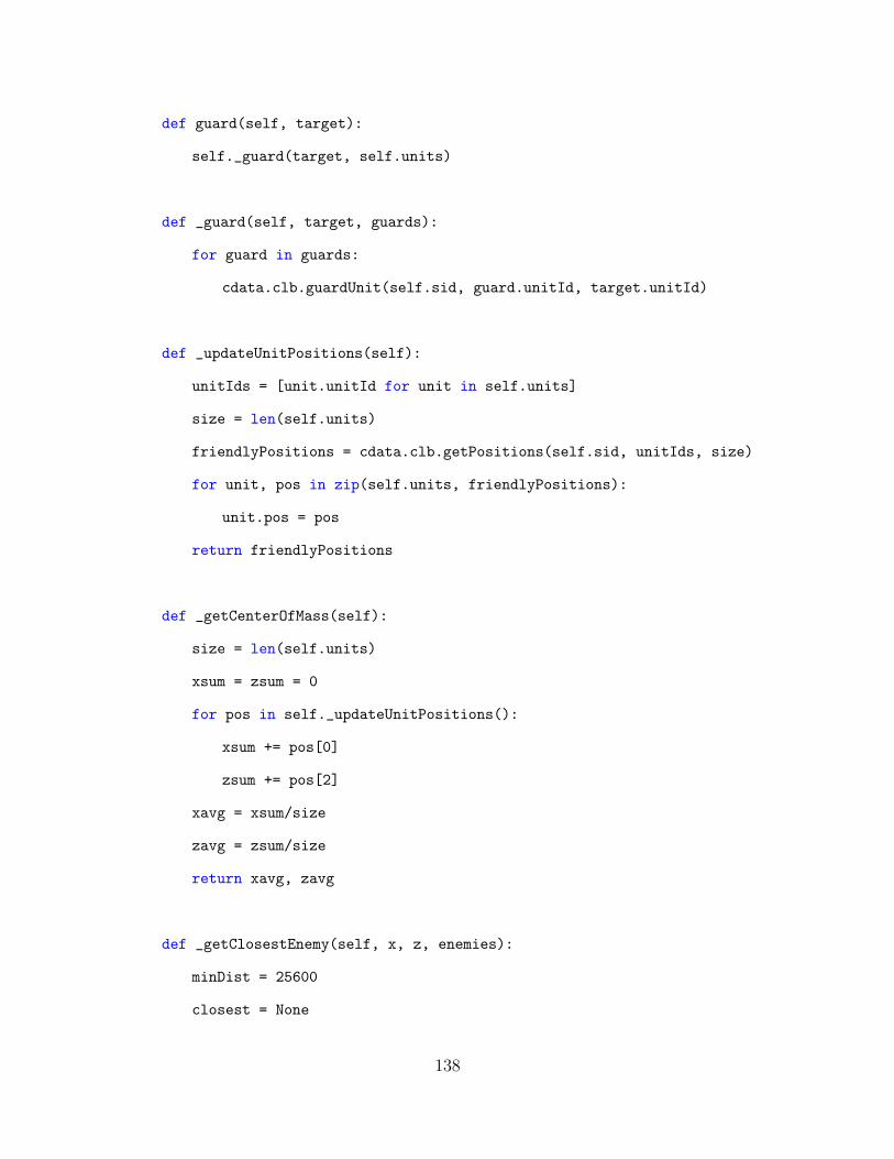
def guard(self, target):
self._guard(target, self.units)
def _guard(self, target, guards):
for guard in guards:
cdata.clb.guardUnit(self.sid, guard.unitId, target.unitId)
def _updateUnitPositions(self):
unitIds = [unit.unitId for unit in self.units]
size = len(self.units)
friendlyPositions = cdata.clb.getPositions(self.sid, unitIds, size)
for unit, pos in zip(self.units, friendlyPositions):
unit.pos = pos
return friendlyPositions
def _getCenterOfMass(self):
size = len(self.units)
xsum = zsum = 0
for pos in self._updateUnitPositions():
xsum += pos[0]
zsum += pos[2]
xavg = xsum/size
zavg = zsum/size
return xavg, zavg
def _getClosestEnemy(self, x, z, enemies):
minDist = 25600
closest = None
138

for enemy in enemies:
dist = calcDist((x, 0.0, z), enemy.pos)
if dist < minDist:
minDist = dist
closest = enemy
return enemy
def calcDist(p1, p2):
’Calculate distance from p1 to p2 in true euclidean coordinates’
return math.sqrt((p2[0] - p1[0])**2 + (p2[2] - p1[2])**2)
class IdleEventFilter:
’Ensures only one idleEvent per group per interval’
def __init__(self):
self.frame = 0
def newEvent(self, group):
if self.frame > group.lastIdleEventFrame:
group.lastIdleEventFrame = self.frame
group.pendingIdleEvent = False
return True
else:
group.pendingIdleEvent = True
return False
139

1.3 agent.py
The agent.py file, located in .config/spring/AI/Skirmish/Tactics/*version*/python,
is changed in order to incorporate the PyGMO software as well as to allow the instant
creation of units for the purpose of analyzing battlefield performance of the tactical
agent. The instant generation of units is performed in the update portion of the
agent.py file, as it is where a time-based command can be implemented. Only the
first portion of the agent.py file is be displayed here as the remainder of the file is
unchanged from the original version.
import ctypes, shelve
import cdata, gamemap, unitmanager, buildmanager, defensemanager,
↪→ attackmanager
import group
from PyGMO import *
from PyGMO.util import *
import moea
# load callback library using ctypes
cdata.clb.saveAgentClb.argtypes = [ctypes.c_int, ctypes.py_object]
class Agent:
def __init__(self, sid, cap):
self.sid = sid # skirmishAI ID number
print ’<Agent {0}> saving callback’.format(sid)
cdata.clb.saveAgentClb(sid, cap) # store callback in library
140

self.frame = 0
if not cdata.unitDefsLoaded:
cdata.loadUnitDefs(sid)
cdata.unitDefsLoaded = True
gamemap.loadMapData(sid)
print ’<Agent {0}> map data loaded’.format(sid)
config = cdata.playerConfigs[sid]
self.collectData = config[1]
strategy = cdata.strategies[config[0]]
# tactics searches config in cdata.py
self.tactics = config[2]
print ’<Agent {0}> has {1} tactic selected’.format(sid, self.tactics
↪→ )
gMap = gamemap.Map(sid)
self.unitManager = unitmanager.UnitManager(sid, gMap)
self.idleEventFlilter = group.IdleEventFilter()
self.attackManager = attackmanager.AttackManager(
sid, self.idleEventFlilter)
# tactics passed to defense manager so it can be passed to group
self.defenseManager = defensemanager.DefenseManager(
sid, strategy, self.attackManager, self.unitManager,
gMap, self.idleEventFlilter, self.tactics)
self.buildManager = buildmanager.BuildManager(
sid, strategy, gMap, self.defenseManager)
cdata.clb.cheat(sid)
self.data = []
def update(self, frame):
141

self.frame = frame
# Quit after 37 minutes
# Number of minutes * 60 sec/min * 30 frame/sec
if frame > 5 * 60 * 30:
self._endGame(’timeup’)
if frame % 5 == 0:
self.idleEventFlilter.frame = frame
self.defenseManager.update(frame)
self.attackManager.update(frame)
if frame % 15 == 0:
self.buildManager.update(frame)
# Write to file every 5 seconds
if self.collectData and frame % (5 * 30) == 0:
self._captureState()
if frame == 30*1:
if self.sid == 0: # tank 155 infantry 123
for i in range(0,25):
cdata.clb.giveUnit(0,(2048,0,900),ctypes.c_int(155))
if self.sid == 1:
for i in range(0,25):
cdata.clb.giveUnit(1,(2048,0,3100),ctypes.c_int(155))
if frame == 30*30:
self.defenseManager.group.setAttacking()
self.attackManager.add(self.defenseManager.group)
self.defenseManager.resetGroup()
142

1.4 config.txt
The config.txt is replaced with a variety of combat focused tactics which allow
for the instantaneous use of the tactical changes in the group.py file to take effect.
Each of the first three lines is focused entirely on producing a certain number of
Stumpy tanks to battle. The final tactic “tac” places 100% effort on economic con-
struction, which means that the commander unit does not construct any new units
throughout the life of the game. This tactic is introduced to facilitate the instanta-
neous army generation used for the online simulation of combat.
# | B E D U|f p r j h w|j f s s p s j|f k t|M S|
5v5 0 0 0 100 0 0 0 0 0 0 0 0 0 0 0 5 0 0 0 0 3 3
13v13 0 0 0 100 0 0 0 0 0 0 0 0 0 0 0 13 0 0 0 0 4 4
25v25 0 0 0 100 0 0 0 0 0 0 0 0 0 0 0 25 0 0 0 0 6 6
tac 0 100 0 0 0 0 0 0 0 0 0 0 0 0 0 5 0 0 0 0 3 3
143

Appendix B. Raw Data for Offline Simulation
This Appendix provides the raw data used for the creation of the tables discussed
in Section 5.3. The appendix is split into three sections: one for each MOEA used.
Each section is split into five subsections which refer to the different population
settings used during the testing of each MOEA. Each subsection begins with a
statement of the average hypervolume found for a single generation which is used
for the remainder of that subsection as the variable 1G. This variable is used in order
to find the values of the average hypervolume increase per second.
2.1 Data for NSGA-II Algorithm
NSGA-II Algorithm Data for 20 Population.
Average Initial Hypervolume for 20 Population (1G) = 98903
Table 9. NSGA-II 20 Population, 2 Generations
Run # obj1 obj2 obj3 obj4 time(s) HV HV-1G (HV-1G)/T
1 1 -5 -441 -41 0.18 108450 9547 53041
2 1 -5 -421 -43 0.18 103175 4272 23735
3 1 -5 -470 -42 0.18 103310 4407 24485
4 1 -4 -387 -49 0.18 108214 9311 51729
5 1 -4 -375 -49 0.18 109460 10557 58652
6 1 -5 -441 -46 0.18 109635 10732 59624
7 1 -5 -475 -50 0.19 119455 20552 108170
8 1 -5 -398 -50 0.18 109925 11022 61235
9 1 -5 -424 -41 0.18 106196 7293 40518
10 1 -5 -447 -49 0.19 110085 11182 58854
avg 1 -4.8 -428 -46 0.18 108791 9888 54004
144

Table 10. NSGA-II 20 Population, 3 Generations
Run # obj1 obj2 obj3 obj4 time(s) HV HV-1G (HV-1G)/T
1 1 -5 -472 -47 0.26 110920 12017 46220
2 1 -5 -410 -50 0.26 113245 14342 55163
3 1 -5 -435 -49 0.24 112295 13392 55801
4 1 -5 -464 -50 0.25 116000 17097 68389
5 1 -5 -410 -50 0.26 114750 15847 60951
6 1 -5 -421 -47 0.26 106275 7372 28355
7 1 -5 -461 -48 0.26 131114 32211 123890
8 1 -4 -381 -49 0.25 109866 10963 43853
9 1 -5 -455 -51 0.26 118155 19252 74047
10 1 -5 -450 -51 0.26 115220 16317 62759
avg 1 -4.9 -436 -49 0.26 114784 15881 61943
Table 11. NSGA-II 20 Population, 4 Generations
Run # obj1 obj2 obj3 obj4 time(s) HV HV-1G (HV-1G)/T
1 1 -5 -458 -53 0.33 123830 24927 75537
2 1 -5 -447 -46 0.33 122025 23122 70068
3 1 -5 -467 -41 0.33 116660 17757 53810
4 1 -5 -432 -50 0.31 117880 18977 61217
5 1 -5 -481 -46 0.33 119880 20977 63568
6 1 -5 -452 -39 0.33 105455 6552 19855
7 1 -5 -458 -39 0.33 125575 26672 80825
8 1 -5 -458 -42 0.33 115658 16755 50774
9 1 -5 -467 -41 0.33 117705 18802 56977
10 1 -5 -404 -50 0.33 113415 14512 43977
avg 1 -5.0 -452 -45 0.33 117808 18906 57661
145

Table 12. NSGA-II 20 Population, 5 Generations
Run # obj1 obj2 obj3 obj4 time(s) HV HV-1G (HV-1G)/T
1 1 -5 -441 -50 0.41 119450 20547 50115
2 1 -5 -450 -50 0.40 115145 56242 140606
3 1 -5 -472 -47 0.41 113070 14167 34554
4 1 -5 -458 -44 0.40 114811 15908 39771
5 1 -5 -410 -55 0.42 125980 27077 64470
6 1 -6 -490 -42 0.41 161620 62717 152968
7 1 -5 -475 -44 0.41 122385 23482 57274
8 1 -5 -464 -55 0.41 130130 31227 76164
9 1 -5 -447 -48 0.39 108330 9427 24173
10 1 -5 -461 -43 0.40 114040 15137 37843
avg 1 -5.1 -457 -48 0.41 126496 27593 67794
146

NSGA-II Algorithm Data for 40 Population.
Average Initial Hypervolume for 40 Population (1G) = 109554
Table 13. NSGA-II 40 Population, 2 Generations
Run # obj1 obj2 obj3 obj4 time(s) HV HV-1G (HV-1G)/T
1 1 -5 -438 -44 0.38 111008 1454 3827
2 1 -4 -358 -47 0.38 104492 -5062 -13320
3 1 -5 -464 -48 0.38 115290 5736 15096
4 1 -5 -435 -45 0.39 106870 -2684 -6881
5 1 -5 -461 -46 0.37 124110 14556 39342
6 1 -5 -478 -45 0.38 109855 301 493
7 1 -5 -432 -48 0.38 109808 254 669
8 1 -5 -390 -52 0.38 120365 10811 28451
9 1 -5 -470 -50 0.37 117500 7946 21477
10 1 -5 -470 -38 0.38 114230 4676 12306
avg 1 -4.9 -440 -46 0.38 113352 3799 10176
Table 14. NSGA-II 40 Population, 3 Generations
Run # obj1 obj2 obj3 obj4 time(s) HV HV-1G (HV-1G)/T
1 1 -5 -418 -65 0.51 150150 40596 79601
2 1 -5 -410 -50 0.52 118170 8616 16570
3 1 -5 -472 -47 0.51 113027 3473 6811
4 1 -5 -464 -50 0.52 117440 7886 15166
5 1 -5 -418 -53 0.51 122660 13106 25699
6 1 -5 -484 -48 0.52 132550 22996 44224
7 1 -5 -458 -52 0.51 120880 11326 22209
8 1 -5 -470 -42 0.52 113685 4131 7945
9 1 -5 -390 -51 0.52 118830 9276 17839
10 1 -6 -498 -51 0.52 170433 60879 117076
avg 1 -5.1 -448 -51 0.52 127782 18229 35314
147

Table 15. NSGA-II 40 Population, 4 Generations
Run # obj1 obj2 obj3 obj4 time(s) HV HV-1G (HV-1G)/T
1 1 -5 -415 -54 0.65 132720 23166 35641
2 1 -5 -458 -51 0.67 121490 11936 17816
3 1 -6 -501 -53 0.65 159318 49764 76561
4 1 -5 -472 -48 0.65 131360 21806 33548
5 1 -6 -501 -47 0.67 157602 48048 71714
6 1 -5 -478 -50 0.67 148740 39186 58487
7 1 -5 -484 -52 0.66 152120 42566 64495
8 1 -5 -467 -49 0.66 128115 18561 28123
9 1 -5 -472 -49 0.67 125010 15456 23069
10 1 -5 -455 -42 0.67 120340 10786 16099
avg 1 -5.2 -470 -50 0.66 137682 28128 42555
Table 16. NSGA-II 40 Population, 5 Generations
Run # obj1 obj2 obj3 obj4 time(s) HV HV-1G (HV-1G)/T
1 1 -5 -470 -55 0.82 158635 49081 59855
2 1 -5 -432 -60 0.80 141320 31766 39708
3 1 -5 -461 -49 0.81 114205 4651 5742
4 1 -5 -467 -52 0.80 174941 65387 81734
5 1 -6 -487 -45 0.81 151890 42336 52267
6 1 -6 -501 -49 0.81 159174 49620 61260
7 1 -6 -495 -60 0.79 178200 68646 86894
8 1 -6 -490 -53 0.81 171064 61510 75939
9 1 -5 -410 -57 0.81 130440 20886 25786
10 1 -5 -467 -45 0.79 118425 8871 11230
avg 1 -5.4 -468 -53 0.81 149829 40276 50042
148

NSGA-II Algorithm Data for 60 Population.
Average Initial Hypervolume for 60 Population (1G) = 110904
Table 17. NSGA-II 60 Population, 2 Generations
Run # obj1 obj2 obj3 obj4 time(s) HV HV-1G (HV-1G)/T
1 1 -5 -401 -54 0.55 132790 21886 39792
2 1 -5 -461 -42 0.56 111650 746 39708
3 1 -5 -464 -45 0.55 120923 10019 18216
4 1 -5 -430 -47 0.56 108870 -2034 -3633
5 1 -5 -455 -47 0.55 127850 16946 30810
6 1 -4 -384 -49 0.56 115536 4632 8271
7 1 -5 -438 -53 0.55 125680 14776 26865
8 1 -4 -380 -51 0.56 114671 3767 6726
9 1 -5 -470 -44 0.56 128185 17281 30858
10 1 -6 -492 -43 0.55 138611 27707 50376
avg 1 -4.9 -438 -48 0.56 122477 11572 20961
Table 18. NSGA-II 60 Population, 3 Generations
Run # obj1 obj2 obj3 obj4 time(s) HV HV-1G (HV-1G)/T
1 1 -5 -472 -51 0.77 122510 11606 15072
2 1 -5 -435 -47 0.77 128870 17966 23332
3 1 -5 -484 -43 0.78 122620 11716 15020
4 1 -5 -441 -49 0.77 114865 3961 5144
5 1 -5 -424 -49 0.78 120100 9196 11789
6 1 -5 -461 -36 0.76 114135 3231 4251
7 1 -6 -487 -46 0.77 134412 23508 30529
8 1 -5 -464 -38 0.77 121760 10856 14098
9 1 -6 -492 -47 0.75 164429 53525 71366
10 1 -5 -470 -49 0.78 119460 8556 10968
avg 1 -5.2 -463 -46 0.77 126316 15412 20157
149

Table 19. NSGA-II 60 Population, 4 Generations
Run # obj1 obj2 obj3 obj4 time(s) HV HV-1G (HV-1G)/T
1 1 -5 -484 -48 1.00 153322 42418 42418
2 1 -5 -472 -44 0.98 127820 16916 17261
3 1 -5 -455 -46 0.99 130095 19191 19384
4 1 -6 -487 -47 0.98 153517 42613 43482
5 1 -4 -381 -53 0.97 124114 13210 13618
6 1 -6 -487 -62 0.97 181164 70260 72433
7 1 -5 -481 -52 0.99 125060 14156 14299
8 1 -6 -501 -50 0.98 162750 51846 52904
9 1 -6 -498 -46 0.98 156712 45808 46742
10 1 -5 -478 -44 1.00 125300 14396 14396
avg 1 -5.3 -472 -49 0.98 143985 33081 33694
Table 20. NSGA-II 60 Population, 5 Generations
Run # obj1 obj2 obj3 obj4 time(s) HV HV-1G (HV-1G)/T
1 1 -5 -475 -56 1.25 144675 33771 27016
2 1 -5 -464 -69 1.23 193544 82640 67187
3 1 -5 -475 -58 1.21 139400 28496 23550
4 1 -5 -481 -59 1.20 141895 30991 25826
5 1 -5 -444 -54 1.20 159100 48196 40163
6 1 -5 -452 -61 1.21 174584 63680 52628
7 1 -4 -338 -63 1.21 182212 71308 58932
8 1 -5 -452 -54 1.20 133405 22501 18751
9 1 -5 -478 -42 1.12 126065 15161 13536
10 1 -6 -504 -53 1.22 160272 49368 40465
avg 1 -5.0 -456 -57 1.21 155515 44611 36805
150

NSGA-II Algorithm Data for 80 Population.
Average Initial Hypervolume for 80 Population (1G) = 112483
Table 21. NSGA-II 80 Population, 2 Generations
Run # obj1 obj2 obj3 obj4 time(s) HV HV-1G (HV-1G)/T
1 1 -6 -498 -63 0.75 188244 75761 101015
2 1 -4 -387 -63 0.76 139768 27285 35902
3 1 -5 -418 -53 0.76 121850 9367 12326
4 1 -5 -432 -47 0.75 121350 8867 11823
5 1 -4 -381 -54 0.75 122106 9623 12831
6 1 -5 -407 -51 0.75 117285 4802 6403
7 1 -5 -475 -53 0.74 128947 16464 22249
8 1 -5 -441 -47 0.76 123615 11132 14648
9 1 -5 -432 -49 0.73 114488 2005 2747
10 1 -5 -455 -49 0.75 111475 -1008 -1343
avg 1 -4.9 -433 -53 0.75 128913 16430 21860
Table 22. NSGA-II 80 Population, 3 Generations
Run # obj1 obj2 obj3 obj4 time(s) HV HV-1G (HV-1G)/T
1 1 -5 -427 -52 1.05 122770 10287 9798
2 1 -5 -338 -52 1.06 149310 36827 34743
3 1 -5 -407 -58 1.06 131470 18987 17913
4 1 -5 -435 -53 1.05 126480 13997 13331
5 1 -5 -472 -48 1.04 139775 27292 26243
6 1 -4 -344 -50 1.04 113996 1513 1455
7 1 -5 -461 -52 1.08 126085 13602 12595
8 1 -5 -407 -50 1.07 121110 8627 8063
9 1 -5 -447 -55 1.05 129690 17207 16388
10 1 -5 -455 -54 1.05 132905 20422 19450
avg 1 -4.9 -419 -52 1.06 129359 16877 15998
151

Table 23. NSGA-II 80 Population, 4 Generations
Run # obj1 obj2 obj3 obj4 time(s) HV HV-1G (HV-1G)/T
1 1 -6 -492 -58 1.35 171216 58733 43506
2 1 -5 -484 -46 1.35 130000 17517 12976
3 1 -5 -455 -54 1.34 129830 17347 12946
4 1 -5 -432 -56 1.39 157520 45037 32401
5 1 -5 -481 -44 1.44 129370 16887 11727
6 1 -6 -492 -45 1.40 173947 61464 43903
7 1 -5 -475 -54 1.37 154835 42352 30914
8 1 -5 -470 -46 1.40 137265 24782 17702
9 1 -5 -441 -58 1.40 138410 25927 18520
10 1 -5 -427 -56 1.42 134165 21682 15269
avg 1 -5.2 -465 -52 1.39 145656 33173 23986
Table 24. NSGA-II 80 Population, 5 Generations
Run # obj1 obj2 obj3 obj4 time(s) HV HV-1G (HV-1G)/T
1 1 -5 -484 -43 1.61 137730 25247 15682
2 1 -6 -487 -48 1.64 166411 53928 32883
3 1 -5 -401 -57 1.63 160609 48126 29525
4 1 -6 -490 -51 1.64 170695 58212 35495
5 1 -6 -495 -47 1.63 153840 41357 25373
6 1 -4 -375 -63 1.64 171165 58682 35782
7 1 -4 -364 -60 1.61 137777 25294 15711
8 1 -6 -501 -55 1.64 197850 85367 34980
9 1 -6 -495 -61 1.65 181170 68687 41629
10 1 -6 -501 -47 1.62 175512 63029 38907
avg 1 -5.4 -459 -53 1.63 162476 49993 30597
152

NSGA-II Algorithm Data for 80 Population.
Average Initial Hypervolume for 80 Population (1G) = 119007
Table 25. NSGA-II 100 Population, 2 Generations
Run # obj1 obj2 obj3 obj4 time(s) HV HV-1G (HV-1G)/T
1 1 -5 -438 -46 0.93 117205 -1802 -1938
2 1 -5 -427 -47 0.93 108965 -10042 -10798
3 1 -5 -450 -52 0.93 121575 2568 2761
4 1 -5 -470 -47 0.92 121455 2448 2661
5 1 -5 -450 -46 0.94 134885 15878 16891
6 1 -4 -384 -49 0.94 112337 -6670 -7096
7 1 -5 -410 -52 0.93 118755 -252 -271
8 1 -5 -472 -45 0.94 124344 5337 5677
9 1 -5 -470 -53 0.93 148420 29413 31627
10 1 -6 -501 -50 0.94 165060 46053 48992
avg 1 -5 -447 -49 0.93 127300 8293 8851
Table 26. NSGA-II 100 Population, 3 Generations
Run # obj1 obj2 obj3 obj4 time(s) HV HV-1G (HV-1G)/T
1 1 -5 -481 -48 1.30 137790 18783 14448
2 1 -5 -467 -49 1.33 127795 8788 6607
3 1 -5 -435 -53 1.32 125205 6198 4695
4 1 -5 -441 -49 1.30 128050 9043 6956
5 1 -4 -364 -59 1.30 132164 13157 10121
6 1 -5 -438 -55 1.32 131545 12538 9498
7 1 -5 -475 -41 1.30 132935 13928 10714
8 1 -5 -410 -54 1.31 130020 11013 8407
9 1 -5 -450 -56 1.32 163974 44967 34066
10 1 -5 -404 -55 1.32 128735 9728 7370
avg 1 -4.9 -437 -52 1.31 133821 14814 11288
153

Table 27. NSGA-II 100 Population, 4 Generations
Run # obj1 obj2 obj3 obj4 time(s) HV HV-1G (HV-1G)/T
1 1 -5 -452 -52 1.73 124515 5508 3184
2 1 -5 -464 -58 1.68 167226 48219 28702
3 1 -5 -464 -49 1.72 151700 32693 19007
4 1 -5 -415 -59 1.71 171650 52643 30785
5 1 -5 -472 -52 1.70 161056 42049 24735
6 1 -5 -424 -60 1.73 175808 56801 32833
7 1 -5 -461 -56 1.70 158801 39794 23408
8 1 -5 -432 -64 1.67 149125 30118 18035
9 1 -6 -490 -49 1.67 184055 65048 38951
10 1 -6 -495 -59 1.69 175230 56223 33268
avg 1 -5.2 -457 -56 1.70 161917 42909 25291
Table 28. NSGA-II 100 Population, 5 Generations
Run # obj1 obj2 obj3 obj4 time(s) HV HV-1G (HV-1G)/T
1 1 -6 -515 -63 2.06 194670 75663 36730
2 1 -6 -504 -51 2.09 181410 62403 29858
3 1 -6 -490 -52 2.06 167886 48879 23728
4 1 -5 -481 -59 2.05 175228 56221 27425
5 1 -6 -510 -50 2.10 211495 92488 44042
6 1 -6 -495 -57 2.05 169290 50283 24528
7 1 -5 -452 -58 2.07 164400 45393 21929
8 1 -6 -498 -51 2.07 157550 38543 18620
9 1 -6 -507 -60 2.05 191286 72279 35258
10 1 -6 -512 -48 2.03 183744 64737 31890
avg 1 -5.8 -496 -55 2.06 179696 60689 29401
154

2.2 Data for SPEA2 Algorithm
SPEA2 Algorithm Data for 20 Population.
Average Initial Hypervolume for 20 Population (1G) = 105714
Table 29. SPEA2 20 Population, 2 Generations
Run # obj1 obj2 obj3 obj4 time(s) HV HV-1G (HV-1G)/T
1 1 -5 -464 -36 0.15 104995 -719 -4795
2 1 -5 -435 -45 0.15 100170 -5544 -36962
3 1 -5 -458 -37 0.14 114160 8446 60326
4 1 -5 -450 -38 0.15 97830 -7884 -52562
5 1 -4 -361 -54 0.15 115834 10120 67465
6 1 -5 -464 -41 0.15 130520 24806 165371
7 1 -5 -450 -40 0.15 106770 1056 7038
8 1 -5 -450 -40 0.15 111580 5866 39105
9 1 -5 -461 -34 0.15 114115 8401 56005
10 1 -4 -378 -48 0.14 108489 2775 19819
avg 1 -4.8 -437 -41 0.15 110446 4732 32081
Table 30. SPEA2 20 Population, 3 Generations
Run # obj1 obj2 obj3 obj4 time(s) HV HV-1G (HV-1G)/T
1 1 -5 -464 -39 0.18 106510 796 4421
2 1 -5 -452 -42 0.18 101670 -4044 -22468
3 1 -5 -418 -54 0.19 120375 14661 77162
4 1 -5 -481 -43 0.19 119165 13451 70794
5 1 -5 -470 -41 0.18 114910 9196 51087
6 1 -5 -461 -39 0.18 112475 6761 37559
7 1 -5 -458 -39 0.18 102885 -2829 -15718
8 1 -5 -458 -41 0.19 100605 -5109 -26891
9 1 -5 -472 -41 0.18 121575 15861 88115
10 1 -5 -461 -35 0.19 116430 10716 56398
avg 1 -5.0 -460 -41 0.18 111660 5946 32046
155

Table 31. SPEA2 20 Population, 4 Generations
Run # obj1 obj2 obj3 obj4 time(s) HV HV-1G (HV-1G)/T
1 1 -5 -467 -42 0.22 116340 10626 48299
2 1 -5 -467 -39 0.22 111195 5481 24912
3 1 -5 -432 -53 0.22 119255 13541 61549
4 1 -5 -441 -60 0.23 137320 31606 137416
5 1 -5 -458 -41 0.22 117340 11626 52844
6 1 -5 -470 -43 0.22 121190 15476 70344
7 1 -4 -350 -49 0.23 108384 2670 11607
8 1 -5 -478 -44 0.22 113635 7921 36003
9 1 -5 -413 -58 0.22 133900 28186 128117
10 1 -4 -330 -57 0.23 125700 19986 86894
avg 1 -4.8 -431 -49 0.22 120426 14712 65799
Table 32. SPEA2 20 Population, 5 Generations
Run # obj1 obj2 obj3 obj4 time(s) HV HV-1G (HV-1G)/T
1 1 -5 -404 -52 0.26 117005 11291 43426
2 1 -5 -470 -49 0.26 117895 12181 46849
3 1 -6 -487 -43 0.25 141836 36122 144487
4 1 -5 -484 -46 0.26 122345 16631 63964
5 1 -5 -481 -55 0.25 144660 38946 155783
6 1 -5 -472 -42 0.26 135975 30261 116387
7 1 -5 -464 -43 0.26 121335 15621 60080
8 1 -5 -478 -50 0.25 128685 22971 91883
9 1 -5 -404 -58 0.26 134565 28851 110964
10 1 -6 -487 -43 0.26 149576 43862 168699
avg 1 -5.2 -463 -48 0.26 131388 25673 100252
156
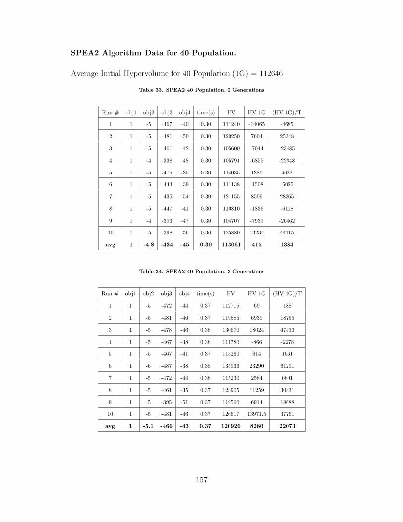
SPEA2 Algorithm Data for 40 Population.
Average Initial Hypervolume for 40 Population (1G) = 112646
Table 33. SPEA2 40 Population, 2 Generations
Run # obj1 obj2 obj3 obj4 time(s) HV HV-1G (HV-1G)/T
1 1 -5 -467 -40 0.30 111240 -14065 -4685
2 1 -5 -481 -50 0.30 120250 7604 25348
3 1 -5 -461 -42 0.30 105600 -7044 -23485
4 1 -4 -338 -48 0.30 105791 -6855 -22848
5 1 -5 -475 -35 0.30 114035 1389 4632
6 1 -5 -444 -39 0.30 111138 -1508 -5025
7 1 -5 -435 -54 0.30 121155 8509 28365
8 1 -5 -447 -41 0.30 110810 -1836 -6118
9 1 -4 -393 -47 0.30 104707 -7939 -26462
10 1 -5 -398 -56 0.30 125880 13234 44115
avg 1 -4.8 -434 -45 0.30 113061 415 1384
Table 34. SPEA2 40 Population, 3 Generations
Run # obj1 obj2 obj3 obj4 time(s) HV HV-1G (HV-1G)/T
1 1 -5 -472 -44 0.37 112715 69 188
2 1 -5 -481 -46 0.37 119585 6939 18755
3 1 -5 -478 -46 0.38 130670 18024 47433
4 1 -5 -467 -38 0.38 111780 -866 -2278
5 1 -5 -467 -41 0.37 113260 614 1661
6 1 -6 -487 -38 0.38 135936 23290 61291
7 1 -5 -472 -44 0.38 115230 2584 6801
8 1 -5 -461 -35 0.37 123905 11259 30431
9 1 -5 -395 -51 0.37 119560 6914 18688
10 1 -5 -481 -46 0.37 126617 13971.5 37761
avg 1 -5.1 -466 -43 0.37 120926 8280 22073
157

Table 35. SPEA2 40 Population, 4 Generations
Run # obj1 obj2 obj3 obj4 time(s) HV HV-1G (HV-1G)/T
1 1 -4 -324 -61 0.46 129675 17029 37021
2 1 -5 -472 -39 0.46 114805 2159 4695
3 1 -5 -478 -43 0.46 125530 12884 28010
4 1 -6 -498 -55 0.45 180475 67829 150732
5 1 -5 -478 -42 0.45 121210 8564 19032
6 1 -5 -438 -53 0.46 124190 11544 25097
7 1 -6 -512 -68 0.45 208896 96250 213890
8 1 -5 -472 -42 0.45 115070 2424 5388
9 1 -5 -455 -52 0.45 126040 13394 29766
10 1 -6 -498 -55 0.45 164340 51694 114877
avg 1 -5.2 -463 -51 0.45 141023 28378 62851
Table 36. SPEA2 40 Population, 5 Generations
Run # obj1 obj2 obj3 obj4 time(s) HV HV-1G (HV-1G)/T
1 1 -6 -495 -66 0.53 196020 83374 157310
2 1 -6 -487 -50 0.54 154920 42274 78286
3 1 -6 -495 -51 0.55 167865 55219 100399
4 1 -5 -464 -39 0.54 121820 9174 16990
5 1 -6 -490 -53 0.54 155820 43174 79953
6 1 -5 -475 -55 0.53 132845 20199 38112
7 1 -6 -492 -56 0.53 165312 52666 99371
8 1 -6 -492 -47 0.54 161135 48489 89795
9 1 -6 -487 -44 0.54 155858 43212 80023
10 1 -5 -484 -45 0.53 134490 21844 41216
avg 1 -5.7 -486 -51 0.54 154609 41963 78146
158

SPEA2 Algorithm Data for 60 Population.
Average Initial Hypervolume for 60 Population (1G) = 109359
Table 37. SPEA2 60 Population, 2 Generations
Run # obj1 obj2 obj3 obj4 time(s) HV HV-1G (HV-1G)/T
1 1 -5 -481 -47 0.47 123715 14356 30546
2 1 -5 -461 -38 0.46 109985 626 1362
3 1 -5 -458 -43 0.47 118655 9296 19780
4 1 -6 -492 -55 0.46 162360 53001 115221
5 1 -5 -447 -47 0.46 110075 716 1558
6 1 -5 -467 -44 0.47 127818 18459 39276
7 1 -5 -478 -45 0.46 129530 20171 43851
8 1 -5 -464 -40 0.47 117120 7761 16514
9 1 -5 -470 -41 0.46 109490 131 286
10 1 -5 -467 -40 0.45 127665 18306 40681
avg 1 -5.1 -469 -44 0.46 123641 14283 30907
Table 38. SPEA2 60 Population, 3 Generations
Run # obj1 obj2 obj3 obj4 time(s) HV HV-1G (HV-1G)/T
1 1 -4 -353 -52 0.58 116203 6844 11801
2 1 -5 -484 -43 0.59 115860 6501 11019
3 1 -5 -475 -46 0.58 141217 31858 54928
4 1 -5 -472 -41 0.59 121170 11811 20019
5 1 -5 -475 -52 0.58 124160 14801 25520
6 1 -5 -472 -39 0.59 126745 17386 29469
7 1 -5 -470 -43 0.58 121270 11911 20537
8 1 -5 -484 -48 0.58 132085 22726 39184
9 1 -5 -464 -46 0.58 120080 10721 18485
10 1 -5 -418 -57 0.59 132220 22861 38748
avg 1 -4.9 -457 -47 0.58 125101 15742 26971
159

Table 39. SPEA2 60 Population, 4 Generations
Run # obj1 obj2 obj3 obj4 time(s) HV HV-1G (HV-1G)/T
1 1 -5 -478 -37 0.68 132990 23631 34752
2 1 -6 -495 -53 0.69 166010 56651 82104
3 1 -6 -495 -47 0.68 165782 56423 82976
4 1 -5 -478 -38 0.69 137950 28591 41437
5 1 -6 -504 -51 0.69 162990 53631 77727
6 1 -5 -461 -62 0.69 143495 34136 49473
7 1 -5 -484 -52 0.69 125840 16481 23886
8 1 -6 -492 -43 0.69 151670 42311 61321
9 1 -5 -481 -42 0.68 121905 12546 18451
10 1 -6 -487 -51 0.68 155257 45898 67498
avg 1 -5.5 -486 -48 0.69 146389 37030 53962
Table 40. SPEA2 60 Population, 5 Generations
Run # obj1 obj2 obj3 obj4 time(s) HV HV-1G (HV-1G)/T
1 1 -5 -484 -44 0.81 144150 34791 42952
2 1 -6 -487 -45 0.81 148764 39405 48649
3 1 -6 -487 -48 0.81 166726 57367 70824
4 1 -6 -492 -54 0.81 175560 66201 81730
5 1 -6 -498 -58 0.81 182070 72711 89767
6 1 -5 -441 -75 0.81 204515 95156 117477
7 1 -5 -432 -66 0.81 191160 81801 100990
8 1 -6 -490 -53 0.81 155820 46461 57360
9 1 -6 -507 -52 0.81 195144 85785 105908
10 1 -6 -490 -50 0.81 156500 47141 58199
avg 1 -5.7 -481 -55 0.81 172041 62862 77386
160

SPEA2 Algorithm Data for 80 Population.
Average Initial Hypervolume for 80 Population (1G) = 114778
Table 41. SPEA2 80 Population, 2 Generations
Run # obj1 obj2 obj3 obj4 time(s) HV HV-1G (HV-1G)/T
1 1 -5 -484 -54 0.62 130680 15902 25648
2 1 -5 -461 -45 0.63 122915 8137 12916
3 1 -4 -347 -54 0.63 120054 5276 8374
4 1 -5 -467 -42 0.62 120570 5792 9342
5 1 -5 -455 -50 0.63 118455 3677 5836
6 1 -5 -467 -45 0.62 122240 7462 12035
7 1 -4 -378 -58 0.62 128757 13979 22547
8 1 -5 -461 -44 0.62 111985 -2793 -4505
9 1 -5 -404 -53 0.62 118370 3592 5793
10 1 -5 -464 -37 0.63 113820 -958 -1521
avg 1 -4.8 -439 -48 0.62 120785 6007 9647
Table 42. SPEA2 80 Population, 3 Generations
Run # obj1 obj2 obj3 obj4 time(s) HV HV-1G (HV-1G)/T
1 1 -5 -484 -40 0.80 141690 26912 33640
2 1 -6 -490 -50 0.80 153705 38927 48659
3 1 -5 -478 -48 0.79 124805 10027 12692
4 1 -5 -470 -44 0.80 125025 10247 12809
5 1 -5 -478 -44 0.80 130575 15797 19746
6 1 -5 -472 -38 0.79 127370 12592 15939
7 1 -5 -481 -44 0.78 119670 4892 6272
8 1 -5 -470 -45 0.79 121440 6662 8433
9 1 -5 -467 -45 0.79 123300 8522 10787
10 1 -6 -487 -54 0.79 157788 43010 54443
avg 1 -5.2 -478 -45 0.79 132537 17759 22342
161

Table 43. SPEA2 80 Population, 4 Generations
Run # obj1 obj2 obj3 obj4 time(s) HV HV-1G (HV-1G)/T
1 1 -5 -447 -62 0.94 148330 33552 35694
2 1 -6 -487 -52 0.95 160204 45426 47817
3 1 -5 -455 -56 0.94 132455 17677 18805
4 1 -5 -484 -61 0.97 147620 32842 33858
5 1 -5 -475 -38 0.95 123215 8437 8881
6 1 -6 -498 -49 0.93 165767 50989 54827
7 1 -5 -478 -43 0.94 125085 10307 10965
8 1 -6 -492 -42 0.93 168449 53671 57711
9 1 -5 -450 -67 0.94 157095 42317 145018
10 1 -6 -498 -58 0.93 193304 78526 84436
avg 1 -5.4 -476 -53 0.94 152152 37374 39801
Table 44. SPEA2 80 Population, 5 Generations
Run # obj1 obj2 obj3 obj4 time(s) HV HV-1G (HV-1G)/T
1 1 -6 -498 -54 1.09 179532 64754 59407
2 1 -6 -507 -52 1.09 176814 62036 56914
3 1 -4 -358 -53 1.07 126104 11326 10585
4 1 -5 -363 -67 1.08 187890 73112 67696
5 1 -6 -492 -49 1.08 160068 45290 41935
6 1 -6 -492 -47 1.08 148144 33366 30894
7 1 -6 -490 -58 1.07 170520 55742 52095
8 1 -6 -487 -48 1.09 152006 37228 34154
9 1 -6 -507 -62 1.08 188604 73826 168357
10 1 -5 -484 -55 1.08 135065 20287 18784
avg 1 -5.6 -468 -55 1.08 162475 47697 44082
162

SPEA2 Algorithm Data for 80 Population.
Average Initial Hypervolume for 80 Population (1G) = 118819
Table 45. SPEA2 100 Population, 2 Generations
Run # obj1 obj2 obj3 obj4 time(s) HV HV-1G (HV-1G)/T
1 1 -5 -432 -53 0.77 121820 3001 3897
2 1 -5 -484 -44 0.77 124145 5326 6917
3 1 -5 -478 -42 0.77 117345 -1474 -1915
4 1 -5 -467 -47 0.76 114385 -4434 -5834
5 1 -5 -484 -46 0.77 124310 5491 7131
6 1 -5 -481 -46 0.77 119010 191 248
7 1 -5 -467 -43 0.77 127885 9066 11774
8 1 -5 -464 -39 0.78 123135 4316 5533
9 1 -5 -467 -44 0.77 117398 -1421 -1846
10 1 -5 -472 -44 0.77 119090 271 352
avg 1 -5.0 -470 -45 0.77 120852 2033 2626
Table 46. SPEA2 100 Population, 3 Generations
Run # obj1 obj2 obj3 obj4 time(s) HV HV-1G (HV-1G)/T
1 1 -6 -490 -48 0.95 153285 34466 36280
2 1 -5 -401 -51 0.97 120576 1757 1811
3 1 -5 -464 -45 0.98 125830 7011 7154
4 1 -5 -481 -46 0.95 121374 2555 2689
5 1 -4 -324 -56 0.97 124223 5404 5571
6 1 -6 -490 -57 0.96 467580 48761 50793
7 1 -5 -472 -52 0.95 122720 3901 4106
8 1 -6 -495 -59 0.97 175230 56411 58155
9 1 -6 -487 -52 0.97 151944 33125 34149
10 1 -5 -472 -52 0.96 129425 10606 11048
avg 1 -5.3 -458 -52 0.96 139219 20400 21176
163

Table 47. SPEA2 100 Population, 4 Generations
Run # obj1 obj2 obj3 obj4 time(s) HV HV-1G (HV-1G)/T
1 1 -5 -481 -44 1.18 143270 24451 20721
2 1 -6 -495 -47 1.18 168035 49216 41708
3 1 -6 -498 -49 1.19 164232 45413 38162
4 1 -6 -490 -43 1.18 168550 49731 42145
5 1 -6 -501 -52 1.18 169542 50723 42985
6 1 -6 -490 -46 1.19 168970 50151 42144
7 1 -6 -492 -48 1.19 161143 42324 35566
8 1 -5 -475 -49 1.18 131630 12811 10857
9 1 -6 -492 -50 1.19 159225 40406 33954
10 1 -5 -481 -49 1.21 134085 15266 12616
avg 1 -5.7 -490 -48 1.19 156868 38049 32086
Table 48. SPEA2 100 Population, 5 Generations
Run # obj1 obj2 obj3 obj4 time(s) HV HV-1G (HV-1G)/T
1 1 -6 -498 -55 1.39 185805 66986 48191
2 1 -6 -492 -65 1.40 193680 74861 53472
3 1 -6 -501 -50 1.40 167118 48299 34499
4 1 -6 -507 -50 1.40 184770 65951 47108
5 1 -6 -524 -57 1.38 183358 64539 46767
6 1 -6 -495 -45 1.38 178089 59270 42949
7 1 -6 -501 -58 1.41 177300 58481 41476
8 1 -6 -504 -54 1.38 163296 44477 32230
9 1 -6 -504 -49 1.41 172656 53837 38182
10 1 -6 -504 -66 1.41 199584 80765 57280
avg 1 -6.0 -503 -55 1.40 180566 61746 44215
164
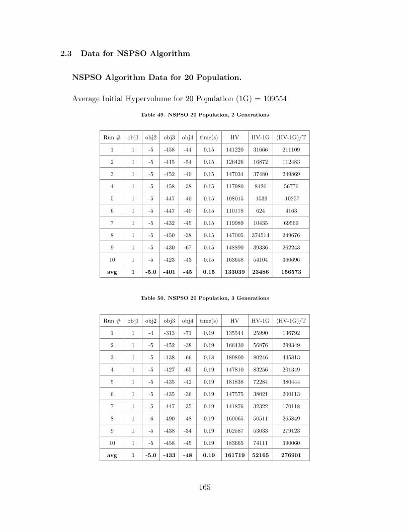
2.3 Data for NSPSO Algorithm
NSPSO Algorithm Data for 20 Population.
Average Initial Hypervolume for 20 Population (1G) = 109554
Table 49. NSPSO 20 Population, 2 Generations
Run # obj1 obj2 obj3 obj4 time(s) HV HV-1G (HV-1G)/T
1 1 -5 -458 -44 0.15 141220 31666 211109
2 1 -5 -415 -54 0.15 126426 16872 112483
3 1 -5 -452 -40 0.15 147034 37480 249869
4 1 -5 -458 -38 0.15 117980 8426 56776
5 1 -5 -447 -40 0.15 108015 -1539 -10257
6 1 -5 -447 -40 0.15 110178 624 4163
7 1 -5 -432 -45 0.15 119989 10435 69569
8 1 -5 -450 -38 0.15 147005 374514 249676
9 1 -5 -430 -67 0.15 148890 39336 262243
10 1 -5 -423 -43 0.15 163658 54104 360696
avg 1 -5.0 -401 -45 0.15 133039 23486 156573
Table 50. NSPSO 20 Population, 3 Generations
Run # obj1 obj2 obj3 obj4 time(s) HV HV-1G (HV-1G)/T
1 1 -4 -313 -71 0.19 135544 25990 136792
2 1 -5 -452 -38 0.19 166430 56876 299349
3 1 -5 -438 -66 0.18 189800 80246 445813
4 1 -5 -427 -65 0.19 147810 83256 201349
5 1 -5 -435 -42 0.19 181838 72284 380444
6 1 -5 -435 -36 0.19 147575 38021 200113
7 1 -5 -447 -35 0.19 141876 32322 170118
8 1 -6 -490 -48 0.19 160065 50511 265849
9 1 -5 -438 -34 0.19 162587 53033 279123
10 1 -5 -458 -45 0.19 183665 74111 390060
avg 1 -5.0 -433 -48 0.19 161719 52165 276901
165

Table 51. NSPSO 20 Population, 4 Generations
Run # obj1 obj2 obj3 obj4 time(s) HV HV-1G (HV-1G)/T
1 1 -4 -381 -55 0.22 204674 94713 430515
2 1 -5 -464 -39 0.22 245750 138021 627370
3 1 -5 -441 -39 0.23 207520 97966 425941
4 1 -5 -475 -39 0.22 205854 96300 437729
5 1 -5 -467 -43 0.22 205682 96128 436947
6 1 -5 -452 -43 0.23 225029 115475 502067
7 1 -5 -438 -40 0.23 194428 84874 369019
8 1 -5 -455 -49 0.23 138552 28998 126080
9 1 -5 -455 -42 0.23 244395 134841 586267
10 1 -5 -421 -44 0.22 203797 94243 428379
avg 1 -4.9 -445 -43 0.23 207710 98156 437031
Table 52. NSPSO 20 Population, 5 Generations
Run # obj1 obj2 obj3 obj4 time(s) HV HV-1G (HV-1G)/T
1 1 -5 -413 -97 0.26 218155 108601 417698
2 1 -5 -452 -38 0.26 578660 469106 1804255
3 1 -5 -447 -40 0.26 259870 150316 578140
4 1 -5 -450 -40 0.26 204249 94695 364213
5 1 -5 -421 -52 0.26 159920 50366 193717
6 1 -5 -438 -44 0.26 242656 133102 511932
7 1 -5 -438 -37 0.26 191349 81795 314598
8 1 -4 -310 -107 0.26 282680 173126 665871
9 1 -5 -447 -93 0.26 210825 101271 389505
10 1 -5 -438 -39 0.26 223432 113878 437994
avg 1 -4.9 -425 -59 0.26 257180 147626 567792
166

NSPSO Algorithm Data for 40 Population.
Average Initial Hypervolume for 40 Population (1G) = 116479
Table 53. NSPSO 40 Population, 2 Generations
Run # obj1 obj2 obj3 obj4 time(s) HV HV-1G (HV-1G)/T
1 1 -5 -464 -49 0.30 119364 2885 9618
2 1 -5 -432 -58 0.30 194984 78505 261684
3 1 -5 -467 -53 0.30 126619 10140 33801
4 1 -5 -447 -38 0.30 124780 8301 27671
5 1 -5 -464 -38 0.30 146947 30468 101561
6 1 -5 -432 -46 0.30 142792 26313 87711
7 1 -5 -441 -46 0.30 169960 53481 178271
8 1 -5 -435 -48 0.30 149255 327766 109254
9 1 -5 -395 -61 0.30 137850 21371 71238
10 1 -5 -430 -46 0.30 151911 35432 118108
avg 1 -5.0 -441 -48 0.30 146446 29968 99892
Table 54. NSPSO 40 Population, 3 Generations
Run # obj1 obj2 obj3 obj4 time(s) HV HV-1G (HV-1G)/T
1 1 -5 -452 -44 0.38 164566 48087 126546
2 1 -5 -450 -39 0.37 204384 87905 237582
3 1 -5 -447 -42 0.38 190670 74191 195240
4 1 -5 -452 -131 0.38 336888 220409 280024
5 1 -5 -461 -41 0.38 177262 60783 159956
6 1 -5 -438 -45 0.38 140363 23884 62853
7 1 -5 -447 -37 0.38 190328 73849 194340
8 1 -5 -421 -46 0.38 169623 531446 139853
9 1 -5 -455 -79 0.38 210770 94291 248135
10 1 -5 -447 -39 0.38 151250 34771 91503
avg 1 -5.0 -447 -54 0.38 193610 77132 203603
167

Table 55. NSPSO 40 Population, 4 Generations
Run # obj1 obj2 obj3 obj4 time(s) HV HV-1G (HV-1G)/T
1 1 -5 -407 -50 0.45 203373 86894 193098
2 1 -5 -444 -39 0.45 222603 106124 235832
3 1 -5 -447 -76 0.46 210055 93576 203427
4 1 -5 -461 -41 0.46 163890 474119 103068
5 1 -5 -467 -46 0.45 644080 527601 1172447
6 1 -5 -455 -47 0.45 234464 117985 262190
7 1 -5 -464 -41 0.45 418131 301652 670338
8 1 -5 -438 -47 0.45 235789 119310 265134
9 1 -5 -438 -68 0.45 218039 101560 225690
10 1 -5 -458 -37 0.45 162000 45521 101158
avg 1 -5.0 -448 -49 0.45 271242 154764 343238
Table 56. NSPSO 40 Population, 5 Generations
Run # obj1 obj2 obj3 obj4 time(s) HV HV-1G (HV-1G)/T
1 1 -5 -455 -39 0.52 286633 170154 327220
2 1 -4 -378 -80 0.52 193030 76551 147214
3 1 -5 -464 -47 0.52 250393 133914 257528
4 1 -5 -484 -45 0.52 670360 553881 1065156
5 1 -5 -455 -94 0.52 490235 373756 718762
6 1 -5 -447 -48 0.52 207438 90959 174922
7 1 -5 -470 -40 0.53 629545 513066 968050
8 1 -5 -455 -46 0.52 262071 145592 279985
9 1 -5 -418 -85 0.52 221457 104978 201881
10 1 -5 -464 -45 0.52 769010 652531 1254868
avg 1 -4.9 -449 -57 0.52 398017 281539 539559
168

NSPSO Algorithm Data for 60 Population.
Average Initial Hypervolume for 60 Population (1G) = 124322
Table 57. NSPSO 60 Population, 2 Generations
Run # obj1 obj2 obj3 obj4 time(s) HV HV-1G (HV-1G)/T
1 1 -5 -452 -40 0.46 167485 43163 77077
2 1 -5 -455 -35 0.46 143869 19547 42493
3 1 -5 -484 -46 0.46 141364 17042 37048
4 1 -5 -413 -56 0.47 164590 40268 85677
5 1 -5 -410 -46 0.46 145710 21388 46496
6 1 -4 -358 -57 0.46 154444 30122 65483
7 1 -5 -452 -40 0.46 152802 28480 61913
8 1 -5 -450 -37 0.46 160783 36461 79263
9 1 -5 -455 -45 0.46 143232 18910 41109
10 1 -5 -452 -47 0.46 132448 8126 17665
avg 1 -4.9 -438 -45 0.46 150673 26351 57098
Table 58. NSPSO 60 Population, 3 Generations
Run # obj1 obj2 obj3 obj4 time(s) HV HV-1G (HV-1G)/T
1 1 -5 -470 -43 0.57 559745 435423 763900
2 1 -5 -447 -82 0.56 191520 67198 119996
3 1 -5 -452 -41 0.57 197630 73308 128611
4 1 -4 -370 -93 0.57 238696 114374 200656
5 1 -5 -455 -83 0.57 198893 74571 130826
6 1 -5 -450 -44 0.57 350500 226178 396803
7 1 -5 -447 -50 0.57 199974 75652 132723
8 1 -5 -467 -43 0.57 167244 42922 75302
9 1 -5 -458 -41 0.57 164423 40101 70353
10 1 -5 -438 -84 0.57 249870 125548 220260
avg 1 -4.9 -445 -60 0.57 251850 127528 223943
169

Table 59. NSPSO 60 Population, 4 Generations
Run # obj1 obj2 obj3 obj4 time(s) HV HV-1G (HV-1G)/T
1 1 -5 -455 -46 0.69 421409 297087 430561
2 1 -4 -301 -120 0.70 303138 178816 255451
3 1 -5 -455 -62 0.69 216815 92493 134048
4 0 -5 -403 -128 0.69 535180 410858 595446
5 1 -5 -455 -36 0.69 245782 121460 176029
6 1 -5 -464 -47 0.68 190204 65882 96885
7 1 -5 -452 -43 0.68 206048 81726 120185
8 0 -5 -429 -120 0.68 530590 406268 597453
9 1 -5 -444 -55 0.68 260449 136127 200187
10 1 -5 -461 -49 0.68 230018 105696 155435
avg 0.8 -4.9 -432 -71 0.69 313963 189641 276168
Table 60. NSPSO 60 Population, 5 Generations
Run # obj1 obj2 obj3 obj4 time(s) HV HV-1G (HV-1G)/T
1 0 -5 -443 -137 0.80 890280 765958 957448
2 0 -5 -430 -197 0.81 893950 769628 950158
3 1 -5 -464 -42 0.81 584933 460611 568656
4 1 -4 -353 -84 0.80 249726 125404 156755
5 1 -5 -461 -43 0.80 314880 190558 238198
6 1 -5 -481 -98 0.80 286014 161692 202115
7 1 -5 -464 -38 0.80 245582 121260 151575
8 1 -5 -470 -71 0.80 552325 428003 535004
9 1 -4 -318 -136 0.81 592323 468001 577779
10 0 -5 -428 -146 0.80 644025 519703 649629
avg 0.7 -4.8 -431 -99 0.80 525404 401082 498732
170

NSPSO Algorithm Data for 80 Population.
Average Initial Hypervolume for 80 Population (1G) = 123996
Table 61. NSPSO 80 Population, 2 Generations
Run # obj1 obj2 obj3 obj4 time(s) HV HV-1G (HV-1G)/T
1 1 -5 -398 -52 0.62 146366 22370 36080
2 1 -5 -432 -46 0.62 156570 32574 52538
3 1 -5 -447 -42 0.62 173935 49939 80546
4 1 -5 -418 -63 0.62 144915 20919 33740
5 1 -5 -478 -43 0.63 149293 25297 40153
6 1 -5 -447 -42 0.62 133192 9196 14832
7 1 -5 -481 -50 0.62 213064 89068 143657
8 1 -5 -472 -61 0.62 143960 19964 32199
9 1 -5 -427 -44 0.62 149530 25534 41183
10 1 -5 -415 -54 0.62 141801 17805 28717
avg 1 -5.0 -442 -50 0.62 155263 31266 50365
Table 62. NSPSO 80 Population, 3 Generations
Run # obj1 obj2 obj3 obj4 time(s) HV HV-1G (HV-1G)/T
1 1 -5 -478 -47 0.77 192955 68959 89557
2 1 -5 -455 -50 0.76 213847 89851 118224
3 1 -5 -455 -43 0.76 209205 85209 112117
4 1 -5 -470 -44 0.77 245793 121797 158177
5 1 -5 -455 -52 0.77 188499 64503 83770
6 1 -4 -344 -91 0.77 203476 79480 103220
7 1 -5 -472 -43 0.77 435517 311521 404572
8 1 -5 -455 -95 0.76 222221 98225 129243
9 1 -5 -464 -40 0.76 160354 36358 478389
10 1 -5 -461 -78 0.76 180855 56859 74814
avg 1 -4.9 -451 -58 0.77 225272 101276 132153
171

Table 63. NSPSO 80 Population, 4 Generations
Run # obj1 obj2 obj3 obj4 time(s) HV HV-1G (HV-1G)/T
1 1 -5 -450 -43 0.92 249986 125990 136945
2 1 -5 -415 -64 0.93 182795 58799 63224
3 1 -5 -484 -69 0.92 244035 120039 130477
4 1 -4 -321 -136 0.93 311386 187390 201494
5 1 -5 -455 -43 0.93 478237 354241 380904
6 1 -5 -452 -51 0.93 469961 345945 372005
7 1 -4 -335 -92 0.92 397459 273463 297242
8 1 -5 -458 -46 0.92 253239 129243 140481
9 0 -4 -317 -135 0.93 555592 431596 464081
10 1 -5 -458 -47 0.92 310789 186793 203035
avg 0.9 -4.7 -415 -73 0.93 345348 221352 238989
Table 64. NSPSO 80 Population, 5 Generations
Run # obj1 obj2 obj3 obj4 time(s) HV HV-1G (HV-1G)/T
1 1 -6 -498 -47 1.09 751468 627472 575662
2 1 -5 -438 -100 1.10 284532 160536 145941
3 1 -5 -461 -49 1.09 261902 137906 126519
4 1 -5 -484 -73 1.10 276066 152070 138245
5 1 -5 -470 -40 1.09 397780 273784 251178
6 1 -5 -461 -85 1.10 209020 85024 77294
7 0 -5 -422 -178 1.10 866485 742489 674990
8 1 -5 -455 -84 1.09 642340 518344 475545
9 1 -4 -341 -112 1.09 503312 379316 347996
10 1 -5 -390 -92 1.10 286631 162635 147850
avg 0.9 -5.0 -442 -86 1.10 447954 323957 296122
172

NSPSO Algorithm Data for 100 Population.
Average Initial Hypervolume for 100 Population (1G) = 123724
Table 65. NSPSO 100 Population, 2 Generations
Run # obj1 obj2 obj3 obj4 time(s) HV HV-1G (HV-1G)/T
1 1 -5 -438 -55 0.78 135498 11774 15095
2 1 -5 -458 -43 0.78 205598 81874 104967
3 1 -4 -333 -67 0.79 141490 17766 22489
4 1 -5 -415 -49 0.79 159528 35804 45322
5 1 -5 -421 -50 0.80 195104 71380 89226
6 1 -5 -458 -48 0.79 158427 34703 43928
7 1 -5 -407 -53 0.78 154015 30291 38835
8 1 -5 -435 -49 0.78 200157 76433 97992
9 1 -5 -467 -40 0.79 160961 37237 47136
10 1 -5 -464 -43 0.78 149820 26096 33457
avg 1 -4.9 -430 -50 0.79 166060 42336 53845
Table 66. NSPSO 100 Population, 3 Generations
Run # obj1 obj2 obj3 obj4 time(s) HV HV-1G (HV-1G)/T
1 1 -5 -481 -45 0.97 602470 478746 493553
2 1 -5 -470 -50 0.97 268878 145154 149644
3 1 -5 -452 -51 0.98 216072 92348 94233
4 0 -5 -445 -147 0.98 711510 587786 599782
5 1 -5 -452 -56 0.98 204359 80635 82281
6 1 -5 -461 -42 0.97 192852 69128 71266
7 1 -4 -358 -100 0.97 266894 143170 147598
8 1 -4 -307 -92 0.97 263127 139403 143715
9 1 -5 -430 -51 0.97 166535 42811 44135
10 1 -4 -318 -112 0.97 241541 117817 121461
avg 0.9 -4.7 -417 -75 0.97 313424 189700 194767
173

Table 67. NSPSO 100 Population, 4 Generations
Run # obj1 obj2 obj3 obj4 time(s) HV HV-1G (HV-1G)/T
1 1 -5 -413 -118 1.17 574872 451148 385597
2 1 -5 -475 -78 1.17 671630 547906 468296
3 1 -5 -450 -107 1.17 274876 151152 129190
4 0 -5 -466 -134 1.17 646220 522496 446578
5 1 -5 -464 -40 1.17 660895 537171 459121
6 1 -5 -461 -48 1.17 565975 442251 377993
7 1 -4 -293 -123 1.17 251849 128125 109509
8 1 -5 -432 -72 1.16 247128 123404 106383
9 1 -5 -472 -43 1.17 545855 422131 360796
10 0 -5 -454 -149 1.17 682760 559036 477809
avg 0.8 -4.9 -438 -91 1.17 512206 388482 332127
Table 68. NSPSO 100 Population, 5 Generations
Run # obj1 obj2 obj3 obj4 time(s) HV HV-1G (HV-1G)/T
1 1 -5 -464 -54 1.37 230114 106390 77657
2 0 -5 -445 -145 1.37 748880 625156 456319
3 0 -5 -466 -137 1.38 687340 563616 408418
4 1 -5 -455 -108 1.37 619980 496256 362231
5 0 -5 -457 -150 1.37 985370 861646 628939
6 1 -5 -481 -42 1.38 645501 521777 378100
7 0 -5 -429 -131 1.37 662890 539166 393552
8 1 -5 -458 -45 1.37 250085 126361 92235
9 1 -5 -452 -44 1.38 284273 160549 116340
10 0 -4 -295 -151 1.38 657199 533475 386576
avg 0.5 -4.9 -440 -101 1.37 577163 453440 330036
174

Appendix C. Raw Data for Online Simulation
This appendix provides the raw win/loss rate and other statistical data acquired
during simulations between various tactical decision making methods on the Spring
RTS engine. For each series of battles the title is in the format “Online Simulation
Results for X Tactic vs Y Tactic”. The “X” tactic begins the battle at the start of
the map, and the “Y” tactic begins on the bottom. There are be 10 battles between
each type of tactic for each method from each direction.
3.1 Data for MOEA Tactic Starting From Top of Map
Table 69. Online Simulation Results for MOEA Tactic vs Default Tactic
Win/Lose Battle Duration # Units Remaining Average Remaining HP
Win 0:32 12 758.17
Win 0:40 5 952.8
Win 0:35 7 793.29
Lose 0:28 15 720.67
Win 0:33 5 339.8
Lose 0:37 9 842.78
Win 0:29 12 1384.08
Win 0:32 10 1150
Win 0:37 8 1275.38
Lose 0:34 12 842.58
175

Table 70. Online Simulation Results for MOEA Tactic vs Proximity Tactic
Win/Lose Battle Duration # Units Remaining Average Remaining HP
Win 0:36 5 664.4
Win 0:28 17 1166.65
Win 0:33 12 920.42
Lose 0:33 13 912.77
Lose 0:46 3 672.33
Win 0:40 4 827.25
Win 0:26 15 1118.13
Lose 0:44 3 669
Lose 0:42 13 783.69
Win 0:45 7 918
Table 71. Online Simulation Results for MOEA Tactic vs Weak Tactic
Win/Lose Battle Duration # Units Remaining Average Remaining HP
Win 0:43 6 1332.5
Win 0:33 8 1105.88
Win 0:33 10 1299.7
Win 0:38 11 1465
Win 0:34 8 1329.63
Win 0:42 5 1150
Win 0:26 15 1141.6
Win 0:37 5 1247.8
Win 0:30 11 1391.73
Win 0:38 7 1396.43
176

3.2 Data for Default Tactic Starting From Top of Map
Table 72. Online Simulation Results for Default Tactic vs MOEA Tactic
Win/Lose Battle Duration # Units Remaining Average Remaining HP
Lose 0:28 8 923.63
Win 0:42 4 903.5
Lose 0:45 4 1008
Lose 0:33 7 778.43
Lose 0:33 8 1144.13
Lose 0:40 5 811.2
Lose 0:35 8 1123.75
Lose 0:29 12 1609.08
Lose 0:26 12 1329.92
Lose 0:25 19 1440.26
177

Table 73. Online Simulation Results for Default Tactic vs Proximity Tactic
Win/Lose Battle Duration # Units Remaining Average Remaining HP
Lose 0:30 10 1096.3
Win 0:37 5 982.6
Win 1:03 2 1007
Lose 0:49 3 418.33
Lose 0:40 5 1251.4
Win 0:56 2 210
Win 0:52 4 894.75
Lose 0:36 8 1010.25
Win 0:41 7 1229.43
Lose 0:42 5 1281
Table 74. Online Simulation Results for Default Tactic vs Weak Tactic
Win/Lose Battle Duration # Units Remaining Average Remaining HP
Win 0:37 7 1268.57
Lose 0:45 7 1215.71
Win 0:37 7 1474.14
Win 0:31 9 1354.89
Win 0:43 4 1401.25
Win 0:45 3 1039
Win 0:41 5 1314.6
Win 0:36 7 1164
Win 0:35 7 1465
Win 0:48 4 1391.25
178

3.3 Data for Proximity Tactic Starting from Top of Map
Table 75. Online Simulation Results for Proximity Tactic vs Default Tactic
Win/Lose Battle Duration # Units Remaining Average Remaining HP
Lose 0:38 11 978.36
Lose 0:46 7 768.86
Lose 0:44 4 653.25
Lose 0:41 5 1112.4
Win 0:42 5 822.2
Lose 0:36 8 1118.38
Lose 0:34 12 1262.42
Lose 0:38 10 1073.2
Win 0:34 7 1184.71
Win 0:45 4 1077
179

Table 76. Online Simulation Results for Proximity Tactic vs MOEA Tactic
Win/Lose Battle Duration # Units Remaining Average Remaining HP
Lose 0:49 7 1213.14
Lose 0:25 14 1066.93
Lose 0:31 11 652.55
Lose 0:34 11 840.82
Lose 1:15 1 49
Win 0:39 4 565
Lose 0:50 5 1448.2
Lose 0:41 8 937.13
Win 0:52 5 815.8
Lose 0:42 7 1210.29
Table 77. Online Simulation Results for Proximity Tactic vs Weak Tactic
Win/Lose Battle Duration # Units Remaining Average Remaining HP
Win 0:46 6 1408.67
Win 0:38 9 1162.11
Win 0.34 10 1522.6
Win 0:49 3 790.33
Win 0:47 3 898.33
Win 0:44 7 1428.71
Win 0:45 8 1090.25
Win 0:44 9 1356.56
Win 0:31 15 1391.13
Win 0:43 8 978.38
180

3.4 Data for Weak Tactic Starting from Top of Map
Table 78. Online Simulation Results for Weak Tactic vs Default Tactic
Win/Lose Battle Duration # Units Remaining Average Remaining HP
Lose 0:37 9 1257.78
Lose 0:39 10 1419.4
Lose 0:35 6 1042.5
Lose 0:36 6 936.67
Lose 0:30 9 1244.22
Lose 0:36 9 1296.67
Lose 0:38 7 1373.14
Lose 0:35 5 1338.2
Win 0:39 7 996.86
Lose 0:34 7 999.57
181

Table 79. Online Simulation Results for Weak Tactic vs Proximity Tactic
Win/Lose Battle Duration # Units Remaining Average Remaining HP
Lose 0:26 15 993.733
Lose 0:34 12 1486.83
Lose 0:44 9 1380.89
Lose 0:34 11 1501.09
Lose 0:55 3 1168.67
Lose 0:43 11 1386
Lose 0:38 12 1353.67
Lose 0:41 11 1200.45
Lose 0:42 6 1152.5
Lose 1:07 1 940
Table 80. Online Simulation Results for Weak Tactic vs MOEA Tactic
Win/Lose Battle Duration # Units Remaining Average Remaining HP
Lose 0:31 14 1098.21
Lose 0:34 11 1346.27
Lose 0:36 8 1124.25
Lose 0:31 11 1549.64
Lose 0:31 12 1500.83
Lose 0:27 15 1455.53
Lose 0:30 10 1269.9
Lose 0:34 11 1380.09
Lose 0:28 12 1299
Lose 0:41 2 776.5
182

Appendix D. Online Simulation Data Sorted by Winner
This appendix takes the data from Appendix C and reorganizes it based on the
simulation’s winner. This helps to compile a quick-look at the statistics attained
when a specific tactic is victorious. Because of this organizational structure, tactics
that lose often do not have as many data points for analysis.
4.1 MOEA Tactic Victory Statistics
Table 81. Statistics for MOEA Tactic Victory against Default Tactic
Battle Duration # Units Remaining Average Remaining HP
0:32 12 758.17
0:40 5 952.8
0:35 7 793.29
0:33 5 339.8
0:29 12 1384.08
0:32 10 1150
0:37 8 1275.38
0:28 8 923.63
0:45 4 1008
0:33 7 778.43
0:33 8 1144.13
0:40 5 811.2
0:35 8 1123.75
0:29 12 1609.08
0:26 12 1329.92
0:25 19 1440.26
183

Table 82. Statistics for MOEA Tactic Victory against Proximity Tactic
Battle Duration # Units Remaining Average Remaining HP
0:36 5 664.4
0:28 17 1166.65
0:33 12 920.42
0:40 4 827.25
0:26 15 1118.13
0:45 7 918
0:49 7 1213.14
0:25 14 1066.93
0:31 11 652.55
0:34 11 840.82
1:15 1 49
0:50 5 1448.2
0:41 8 937.13
0:42 7 1210.29
184

Table 83. Statistics for MOEA Tactic Victory against Weak Tactic
Battle Duration # Units Remaining Average Remaining HP
0:43 6 1332.5
0:33 8 1105.88
0:33 10 1299.7
0:38 11 1465
0:34 8 1329.63
0:42 5 1150
0:26 15 1141.6
0:37 5 1247.8
0:30 11 1391.73
0:38 7 1396.43
0:31 14 1098.21
0:34 11 1346.27
0:36 8 1124.25
0:31 11 1549.64
0:31 12 1501.83
0:27 15 1455.53
0:30 10 1269.9
0:34 11 1380.1
0:28 12 1299
0:41 2 776.5
185

4.2 Default Tactic Victory Statistics
Table 84. Statistics for Default Tactic Victory against MOEA Tactic
Battle Duration # Units Remaining Average Remaining HP
0:28 15 720.67
0:37 9 842.78
0:34 12 841.58
0:42 4 903.5
Table 85. Statistics for Default Tactic Victory against Proximity Tactic
Battle Duration # Units Remaining Average Remaining HP
0:37 5 982.6
1:03 2 1007
0:56 2 210
0:52 4 894.75
0:41 7 1229.43
0:38 11 978.36
0:46 7 768.86
0:44 4 653.25
0:41 5 1112.4
0:36 8 1118.38
0:34 12 1262.42
0:38 10 1073
186

Table 86. Statistics for Default Tactic Victory against Weak Tactic
Battle Duration # Units Remaining Average Remaining HP
0:37 7 1268.57
0:37 7 1474.14
0:31 9 1354.89
0:43 4 1401.25
0:45 3 1039
0:41 5 1314.6
0:36 7 1164
0:35 7 1465
0:48 4 1391.25
0:37 9 1257.78
0:39 10 1419.4
0:35 6 1042.5
0:36 6 936.67
0:30 9 1244.22
0:36 9 1296.67
0:38 7 1373.14
0:35 5 1338.2
0:34 7 999.57
187

4.3 Proximity Tactic Victory Statistics
Table 87. Statistics for Proximity Tactic Victory against MOEA Tactic
Battle Duration # Units Remaining Average Remaining HP
0:33 13 912.77
0:46 3 672.33
0:44 3 669
0:42 13 783.69
0:39 4 565
0:52 5 815.8
Table 88. Statistics for Proximity Tactic Victory against Default Tactic
Battle Duration # Units Remaining Average Remaining HP
0:30 10 1096.3
0:49 3 418.33
0:40 5 1251.4
0:36 8 1010.25
0:42 5 1281
0:42 5 822.2
0:34 7 1184.71
0:45 4 1077
188

Table 89. Statistics for Proximity Tactic Victory against Weak Tactic
Battle Duration # Units Remaining Average Remaining HP
0:46 6 1408.67
0:38 9 1162.11
0:34 10 1522.6
0:49 3 790.33
0:47 3 898.33
0:44 7 1428.71
0:45 8 1090.25
0:44 9 1356.56
0:31 15 1391.13
0:43 8 978.38
0:26 15 993.73
0:34 12 1486.83
0:44 9 1380.89
0:34 11 1501.09
0:55 3 1168.67
0:43 11 1386
0:38 12 1353.67
0:41 11 1200.45
0:42 6 1152.5
1:07 1 940
189

4.4 Weak Tactic Victory Statistics
Table 90. Statistics for Weak Tactic Victory against MOEA Tactic
Battle Duration # Units Remaining Average Remaining HP
N/A N/A N/A
Table 91. Statistics for Weak Tactic Victory against Default Tactic
Battle Duration # Units Remaining Average Remaining HP
0:45 7 1215.71
0:39 7 996.86
Table 92. Statistics for Weak Tactic Victory against Proximity Tactic
Battle Duration # Units Remaining Average Remaining HP
N/A N/A N/A
190

Bibliography
1. John R. Boyd, “The essence of winning and losing,” http://www.danford.net/
boyd.essence.htm, Accessed: March 10, 2015.
2. Alan Sartori-Angus, “Cosmic conquest,” BYTE Magazine, p. 124, December
1982.
3. “Nostalgia series: Dune II,” http://www.rtsguru.com/game/101/article/
123/Nostalgia-Series-Dune-2.html, Accessed: March 10, 2015.
4. “Warcraft: From 1994 to WoW wrath of the lich
king,” http://www.pcgameshardware.com/aid,669750/
Warcraft-From-1994-to-WoW-Wrath-of-the-Lich-King-game-classics-in-series/
News/, Accessed: March 10, 2015.
5. Jason M Blackford, “Online build-order optimization for real-time strategy agents
using multi-objective evolutionary algorithms,” M.S. thesis, Air Force Institute
of Technology, 2014.
6. Lyall J Di Trapani, “A real-time strategy agent framework and strategy classifier
for computer generated forces,” M.S. thesis, Air Force Institution of Technology,
2012.
7. “Multi-objective optimization - wikipedia, the free encyclopedia,” http://en.
wikipedia.org/wiki/Multi-objective_optimization, Accessed: March 10,
2015.
8. “Real-time strategy - wikipedia, the free encyclopedia,” http://en.wikipedia.
org/wiki/Real-time_strategy, Accessed: March 10, 2015.
191

9. “Air education and training command,” http://www.aetc.af.mil/, Accessed:
March 10, 2015.
10. Strategy World, Air Force Wargaming is Different, March 10, 2015.
11. Glen Robertson and Ian Watson, “A review of real-time strategy game AI,” AI
Magazine, vol. 35, no. 4, pp. 75–104, 2014.
12. “Ai script - starcraft and starcraft II wiki,” http://starcraft.wikia.com/
wiki/AI_script, Accessed: March 10, 2015.
13. David Churchill, Abdallah Saffidine, and Michael Buro, “Fast heuristic search
for rts game combat scenarios.,” in Artificial Intelligence and Interactive Digital
Entertainment, 2012.
14. “Starcraft AIb competition,” http://webdocs.cs.ualberta.ca/~cdavid/
starcraftaicomp/, Accessed: March 10, 2015.
15. Malcolm Gladwell, Blink: The power of thinking without thinking, Hachette
Digital, Inc., 2007.
16. “Welcome to the officer training school homepage,” http://www.au.af.mil/au/
holmcenter/OTS/index.asp, Accessed: March 10, 2015.
17. “Welcome to the air university,” http://www.au.af.mil/au/soc/sos.asp, Ac-
cessed: March 10, 2015.
18. David G. Ullman, “OO-OO-OO! the sound of a broken OODA loop,” Crosstalk
- The Journal of Defense Software Engineering, pp. 22–25, 2007.
19. “Dune II - wikipedia, the free encyclopedia,” http://en.wikipedia.org/wiki/
Dune_II, Accessed: March 10, 2015.
192
20. Bob Bates, Game Developer’s Market Guide (Game Development), Muska &
Lipman/Premier-Trade, 2003.
21. Blizzard Entertainment, “Blizzard entertainment: Classic games,” http://us.
blizzard.com/en-us/games/legacy, Accessed: March 10, 2015.
22. “Wargus — home,” www.wargus.sourceforge.net, Accessed: March 10, 2015.
23. “Stratagus — a real time strategy engine,” www.stratagus.com, Accessed:
March 10, 2015.
24. “Sparcraft - starcraft combat simulation,” https://code.google.com/p/
sparcraft/, Accessed: March 10, 2015.
25. “Spring rts engine,” http://springrts.com, Accessed: March 10, 2015.
26. Carl Von Clausewitz, On war, Digireads.com Publishing, 2004.
27. Ljubica Erickson and Mark Erickson, Russia: war, peace and diplomacy-essays
in honour of John Erickson, Weidenfeld & Nicolson, 2005.
28. “[interviews] bisu, coach park, and jaedong,” http://www.teamliquid.net/
forum/news-archive/339200-interviews-bisu-coach-park-and-jaedong,
Accessed: March 10, 2015.
29. Kurt Weissgerber, “Developing an effective and efficient real time strategy agent
for use as a computer generated force,” M.S. thesis, Air Force Institute of Tech-
nology, 2010.
30. Raul Lara-Cabrera, Carlos Cotta, and Antonio J Fernandez-Leiva, “A review
of computational intelligence in RTS games,” in Foundations of Computational
Intelligence (FOCI), 2013 IEEE Symposium on. IEEE, 2013, pp. 114–121.
193

31. Stuart Russel, Peter Norvig, et al., “Artificial intelligence: A modern approach,
1995,” Cited on, p. 20, 1994.
32. David W Aha, Matthew Molineaux, and Marc Ponsen, “Learning to win: Case-
based plan selection in a real-time strategy game,” in Case-based reasoning re-
search and development, pp. 5–20. Springer, 2005.
33. Santiago Ontanon, Gabriel Synnaeve, Alberto Uriarte, Florian Richoux, David
Churchill, and Mike Preuss, “A survey of real-time strategy game AI research and
competition in starcraft,” Computational Intelligence and AI in Games, IEEE
Transactions on, vol. 5, no. 4, pp. 293–311, 2013.
34. David Churchill and Michael Buro, “Portfolio greedy search and simulation for
large-scale combat in starcraft,” in Computational Intelligence in Games (CIG),
2013 IEEE Conference on. IEEE, 2013, pp. 1–8.
35. Guillaume Chaslot, Monte-carlo tree search, Ph.D. thesis, Maastricht University,
2010.
36. A Fernandez-Ares, P Garcıa-Sanchez, AM Mora, PA Castillo, and JJ Merelo,
“Designing competitive bots for a real time strategy game using genetic program-
ming,” http://ceur-ws.org/Vol-1196/cosecivi14_submission_24.pdf, Ac-
cessed: March 10, 2015.
37. Ben George Weber, Michael Mateas, and Arnav Jhala, “Building human-level AI
for real-time strategy games.,” in AAAI Fall Symposium: Advances in Cognitive
Systems, 2011.
38. Marius Stanescu, Nicolas A Barriga, and Michael Buro, “Hierarchical adversarial
search applied to real-time strategy games,” in Tenth Annual AAAI Conference
on Artificial Intelligence and Interactive Digital Entertainment (AIIDE), 2014.
194

39. Carlos Coello Coello, Gary B Lamont, and David A Van Veldhuizen, Evolutionary
algorithms for solving multi-objective problems, 2nd edition, Springer Science &
Business Media, 2007.
40. Swiss Federal Institute of Technology Zurich, “Dtlz2 test problems,” http://
www.tik.ee.ethz.ch/sop/download/supplementary/testproblems/dtlz2/,
note=Accessed: March 10, 2015.
41. Kalyanmoy Deb, Amrit Pratap, Sameer Agarwal, and TAMT Meyarivan, “A fast
and elitist multiobjective genetic algorithm: NSGA-II,” Evolutionary Computa-
tion, IEEE Transactions on, vol. 6, no. 2, pp. 182–197, 2002.
42. Eckart Zitzler and Lothar Thiele, “Multiobjective evolutionary algorithms: a
comparative case study and the strength pareto approach,” Evolutionary Com-
putation, IEEE Transactions on, vol. 3, no. 4, pp. 257–271, 1999.
43. Eckart Zitzler, Marco Laumanns, Lothar Thiele, Eckart Zitzler, Eckart Zitzler,
Lothar Thiele, and Lothar Thiele, “SPEA2: Improving the strength pareto evo-
lutionary algorithm,” 2001.
44. Yang Liu, “A fast and elitist multi-objective particle swarm algorithm: NSPSO,”
in Granular Computing, 2008. GrC 2008. IEEE International Conference on.
IEEE, 2008, pp. 470–475.
45. N Chase, M Rademacher, E Goodman, R Averill, and R Sidhu, “A benchmark
study of multi-objective optimization methods,” Tech. Rep., Red Cedar Technol-
ogy.
46. R Timothy Marler and Jasbir S Arora, “Survey of multi-objective optimization
methods for engineering,” Structural and multidisciplinary optimization, vol. 26,
no. 6, pp. 369–395, 2004.
195

47. David H Wolpert and William G Macready, “No free lunch theorems for opti-
mization,” Evolutionary Computation, IEEE Transactions on, vol. 1, no. 1, pp.
67–82, 1997.
48. El-Ghazali Talbi, Metaheuristics: from design to implementation, vol. 74, John
Wiley & Sons, 2009.
49. “jMetal web site,” http://jmetal.sourceforge.net/, Accessed: March 10,
2015.
50. “MOEA framework, a java library for multi-objective evolutionary algorithms,”
http://www.moeaframework.org/, Accessed: March 10, 2-15.
51. “Welcome to PyGMO,” http://esa.github.io/pygmo/, Accessed: March 10,
2015.
52. “ParadisEO, paradiseo home page,” http://paradiseo.gforge.inria.fr/, Ac-
cessed: March 10, 2015.
53. Arnaud Liefooghe, Laetitia Jourdan, and El-Ghazali Talbi, “A software frame-
work based on a conceptual unified model for evolutionary multiobjective opti-
mization: Paradiseo-moeo,” European Journal of Operational Research, vol. 209,
no. 2, pp. 104–112, 2011.
54. “Borg MOEA, a high-performance, robust, adaptive multi-objective evolutionary
algorithm,” www.borgmoea.org, Accessed: March 10, 2015.
55. “MOEA software availability,” http://www.cs.cinvestav.mx/~emoobook/
apendices/appendix-h.pdf, Accessed: March 10, 2015.
56. Carlos A Coello Coello, “Software,” http://delta.cs.cinvestav.mx/
~ccoello/EMOO/EMOOsoftware.html, Accessed March 10, 2015.
196

57. “Balanced annihilation - spring,” https://springrts.com/wiki/Balanced_
Annihilation, Accessed: March 10, 2015.
58. “Multi-objective optimization - wikipedia, the free encyclopedia,” http://en.
wikipedia.org/wiki/Multi-objective_optimization, Accessed: March 10,
2015.
59. “Quick start - PyGMO 1.1.5 documentation,” http://esa.github.io/pygmo/
quickstart.html, Accessed: March 10, 2015.
60. “Fog of war - wikipedia, the free encyclopedia,” http://en.wikipedia.org/
wiki/Fog_of_war, Accessed: March 10, 2015.
61. Alexander Kovarsky and Michael Buro, “Heuristic search applied to abstract
combat games,” in Advances in Artificial Intelligence, pp. 66–78. Springer, 2005.
62. “Balanced annihilation v7.60 - armstump,” http://imolarpg.dyndns.org/
modinfo/ba760/armstump.html, Accessed: March 10, 2015.
63. Peter Sarkozy, “Balanced annihilation mod info,” http://
balancedannihilation.org/modinfo/, Accessed: March 10, 2015.
64. Radha-Krishna Balla and Alan Fern, “UCT for tactical assault planning in real-
time strategy games.,” in International Joint Conferences on Artificial Intelli-
gence, 2009, pp. 40–45.
197

REPORT DOCUMENTATION PAGE Form ApprovedOMB No. 0704–0188
The public reporting burden for this collection of information is estimated to average 1 hour per response, including the time for reviewing instructions, searching existing data sources, gathering andmaintaining the data needed, and completing and reviewing the collection of information. Send comments regarding this burden estimate or any other aspect of this collection of information, includingsuggestions for reducing this burden to Department of Defense, Washington Headquarters Services, Directorate for Information Operations and Reports (0704–0188), 1215 Jefferson Davis Highway,Suite 1204, Arlington, VA 22202–4302. Respondents should be aware that notwithstanding any other provision of law, no person shall be subject to any penalty for failing to comply with a collectionof information if it does not display a currently valid OMB control number. PLEASE DO NOT RETURN YOUR FORM TO THE ABOVE ADDRESS.
1. REPORT DATE (DD–MM–YYYY) 2. REPORT TYPE 3. DATES COVERED (From — To)
4. TITLE AND SUBTITLE 5a. CONTRACT NUMBER
5b. GRANT NUMBER
5c. PROGRAM ELEMENT NUMBER
5d. PROJECT NUMBER
5e. TASK NUMBER
5f. WORK UNIT NUMBER
6. AUTHOR(S)
7. PERFORMING ORGANIZATION NAME(S) AND ADDRESS(ES) 8. PERFORMING ORGANIZATION REPORTNUMBER
9. SPONSORING / MONITORING AGENCY NAME(S) AND ADDRESS(ES) 10. SPONSOR/MONITOR’S ACRONYM(S)
11. SPONSOR/MONITOR’S REPORTNUMBER(S)
12. DISTRIBUTION / AVAILABILITY STATEMENT
13. SUPPLEMENTARY NOTES
14. ABSTRACT
15. SUBJECT TERMS
16. SECURITY CLASSIFICATION OF:
a. REPORT b. ABSTRACT c. THIS PAGE
17. LIMITATION OFABSTRACT
18. NUMBEROFPAGES
19a. NAME OF RESPONSIBLE PERSON
19b. TELEPHONE NUMBER (include area code)
Standard Form 298 (Rev. 8–98)Prescribed by ANSI Std. Z39.18
26-03-2015 Master’s Thesis Sept 2013 — Mar 2015
Tactical AI InReal Time Strategy Games
Gruber, Donald A., Capt, USAF
Air Force Institute of TechnologyGraduate School of Engineering and Management (AFIT/EN)2950 Hobson WayWPAFB OH 45433-7765
AFIT-ENG-MS-15-M-021
Intentionally Left Blank
Distribution Statement A:Approved for Public Release; Distribution Unlimited.
This material is declared a work of the U.S. Government and is not subject to copyright protection in the United States
The real time strategy (RTS) tactical decision making problem is a difficult problem. It is generally more complex due toits high degree of time sensitivity. This research effort presents a novel approach to this problem within an educational,teaching objective. Particular decision focus is target selection for a artificial intelligence (AI) RTS game model. The useof multi-objective evolutionary algorithms (MOEAs) in this tactical decision making problem allows an AI agent to makefast, effective solutions that do not require modification to fit the current environment. This approach allows for thecreation of a generic solution building tool that is capable of performing well against scripted opponents withoutrequiring expert training or deep tree searches. The experimental results validate that MOEAs can control an on-lineagent capable of out performing a variety AI RTS opponent test scripts.
RTS, Tactics, MOEA, Optimization
U U U UU 218
Dr. G. B. Lamont, AFIT/ENG
(937) 255-3636, x4718; [email protected]