Embed Size (px)
Citation preview

TABLE OF CONTENTS
Section and Page Number
A. Brief Review of Topics from Micro & Macro Principles, 2
B. Detailed Review of Topics from Micro & Macro Principles, 5
C. Intermediate Microeconomics Study Guide, 31
D. Intermediate Macroeconomics Review: Sample Problem Set
with Solutions, 60
E. International Economics Review
1. Overview of International Economics, 69
2. Welfare Effects of a Tariff, 74
3. How the Exchange Rate Affects Trade Patterns, 76
4. The Balance of Payments, 78
5. More International Finance, 79

Brief Review of
Topics from Micro & Macro Principles
Microeconomics
Definition of economics, microeconomics, macroeconomics
Points to remember when evaluating problems using economic analysis
Positive vs. Normative economics
Opportunity Cost
Production Possibilities Curve
Specialization & Trade according to the law of comparative advantage
Economic efficiency = technical & allocative
Theory of Exchange
3 basic economic questions
3 basic institutional arrangements used to answer economic questions = market, political, social
Property rights as a complement to the market process
Adam Smith – invisible hand
Selfish vs. self-interest
3 criteria used to evaluate market, political & social processes = equity/fairness, efficiency,
liberty
Rational behavior
Scarcity competition rationing discrimination
Markets
Relative vs. Monetary prices
Law of demand
Law of supply
Demand & supply shifters
Equilibrium, shortages & surpluses
How markets return to equilibrium if actual price is above or below equilibrium price
Functions of prices
Elasticity: P elasticity of demand
P elasticity of supply
Income elasticity
Short-run business decisions:
Short-run cost curves
Profit maximizing or loss minimizing level of output (Q*)
Shut-down point
Long-run business decisions:
Long-run cost curves
Market structures = Pure Competition, Monopoly, Oligopoly
Economic efficiency within each type of market structure
Macroeconomics
Rationale for using political process to solve economic questions:
I Production Decisions:
Lack of competition
Externalities Public goods } Market Failure
Poor Information
Economic Instability
II Redistribution of Income:
Problems with political process
Employment Act of 1946
Output = GDP:
(A) Expenditure Approach GDP = C + I + G + NE
(B) Income Approach NI = wages & salaries + interest + rents + profits
Differences between GDP & NI
Real vs. Nominal GDP
Problems with GDP as a measure of output
Price indices:
GDP deflator, CPI, PPI
Laspeyres vs. Paasche index
Problems with using p indices to measure changes in prices

Inflation, πt = Pt – Pt – 1 where P = P index
P t - 1
Effects of inflation on economy
Hyperinflation
Unemployment, u = no. unemployed where LF = U + E
LF
Frictional, structural, & cyclical U Full employment
Problems with using U to measure labor market conditions
Business Cycles
Natural Rate of U vs. Actual Rate of U
Potential GDP vs. Actual GDP
Goods and Services Market:
AD & AS curves, equilibrium, AD & AS shifters
Labor Market
Money Market - MD + MS curves
Credit Market – MD depends on income, interest rates & institutional factors
Definition of Money
Function of Money
Nominal vs. Real Money
Federal Reserve System:
12 district banks
Board of Governors
Federal Open Market Committee (FOMC)
Member banks
Banking system = money creation
Equation of exchange
Neutrality of money
Fiscal policy = definition, how it affects economy, effectiveness
Monetary policy = definition, how it affects economy, effectiveness
Int’l Trade = effects of tariffs, quotas, & voluntary exchange restrictions

Detailed Review of
Topics from Micro & Macro Principles Economics: A social science investigating the optimal allocation of scarce resources subject to certain constraints. Scarcity: There are not enough resources to produce everything everybody wants. Constraints: Scarcity forces trade-offs with respect to means (income). Factors of Production = Resources = Land, Labor, Physical Capital and Human Capital Circular Flow Diagram: Sectors: Households, Firms, Government, Financial, Foreign Equilibrium Condition: Leakages (S,T,IM) = Injections (I,G,EX) Micro: Analysis of each individual sector Macro: Analysis of the economy as a whole Criteria for judging economic outcomes: Positive (objective, "is"): Efficiency (Pareto), Growth, Stability Normative (subjective, "should"): Equity, Ethics Modeling Assumptions: 1. Ceteris Paribus 2. Free Will 3. More is better 4. Self interested behavior (not selfish!) Part I: Brief Review of Micro and Macro Economics Principles–Microeconomics
Definition of economics, microeconomics, macroeconomics
Points to remember when evaluating problems using economic analysis
Positive vs. Normative economics
Opportunity Cost
Production Possibilities Curve
Specialization & Trade according to the law of comparative advantage
Economic efficiency = technical & allocative
Theory of Exchange
3 basic economic questions
3 basic institutional arrangements used to answer economic questions = market, political, social
Property rights as a complement to the market process
Adam Smith – invisible hand
Selfish vs. self-interest
3 criteria used to evaluate market, political & social processes = equity/fairness, efficiency, liberty
Rational behavior

Principles of Economics, p. 2
Scarcity competition rationing discrimination
Markets
Relative vs. Monetary prices
Law of demand
Law of supply
Demand & supply shifters
Equilibrium, shortages & surpluses
How markets return to equilibrium if actual price is above or below equilibrium price
Functions of prices
Elasticity: P elasticity of demand
P elasticity of supply
Income elasticity
Short-run business decisions:
Short-run cost curves
Profit maximizing or loss minimizing level of output (Q*)
Shut-down point
Long-run business decisions:
Long-run cost curves
Market structures = Pure Competition, Monopoly, Oligopoly
Economic efficiency within each type of market structure
Macroeconomics
Rationale for using political process to solve economic questions:
I Production Decisions:
Lack of competition
Externalities Public goods
} Market Failure
Poor Information
Economic Instability
II Redistribution of Income:
Problems with political process
Employment Act of 1946
Output = GDP:
(A) Expenditure Approach GDP = C + I + G + NE
(B) Income Approach NI = wages & salaries + interest + rents + profits
Differences between GDP & NI

Principles of Economics, p. 3
Real vs. Nominal GDP
Problems with GDP as a measure of output
Price indices:
GDP deflator, CPI, PPI
Laspeyres vs. Paasche index
Problems with using p indices to measure changes in prices
Inflation, πt = Pt – Pt – 1 where P = P index
P t - 1
Effects of inflation on economy
Hyperinflation
Unemployment, u = no. unemployed where LF = U + E
LF
Frictional, structural, & cyclical U Full employment
Problems with using U to measure labor market conditions
Business Cycles
Natural Rate of U vs. Actual Rate of U
Potential GDP vs. Actual GDP
Goods and Services Market:
AD & AS curves, equilibrium, AD & AS shifters
Labor Market
Money Market - MD + MS curves
Credit Market – MD depends on income, interest rates & institutional factors
Definition of Money
Function of Money
Nominal vs. Real Money
Federal Reserve System:
12 district banks
Board of Governors
Federal Open Market Committee (FOMC)
Member banks
Banking system = money creation
Equation of exchange
Neutrality of money
Fiscal policy = definition, how it affects economy, effectiveness
Monetary policy = definition, how it affects economy, effectiveness
Int’l Trade = effects of tariffs, quotas, & voluntary exchange restrictions

Principles of Economics, p. 4
Part II: More Detailed Review of Micro and Macro Economics Principles– COSTS: Total Cost = Accounting Costs + Opportunity Costs Opportunity Costs: Costs associated with forgoing the next best alternative.
Each decision to produce a good or service means that the resources necessary for production are diverted from their next best use.
Examples: 1. Building a mall on a lake. 2. Going to a Basketball Game. 3. College Education. 4. Urban Sprawl 5. Investment in Capital versus Consumption goods.
Investment in private or public infrastructure leads to sustained growth and increased efficiency. It is a more appropriate long run goal. Soviets invested in bridges, roads, factories and obtained very high growth rates for many years. They fell behind in part due to the fact that by eliminating privatization, they eliminated the incentives for innovation. People were told to sacrifice consumption goods for the good of their children's future.
Production Possibilities Frontier: Locus of all feasible, efficient production possibilities. Illustrates the trade-offs (opportunity costs) associated with the production of two (or more) goods, given the factors of production available to a society. Represents Technical Efficiency.

Principles of Economics, p. 5
Example: Spending on Infrastructure versus Health Care Spending
.A
BC
D.. .roads
health care
A&C: efficient, B: inefficient (some factors are unemployed), D: not feasible or unattainable Marginal Rate of Transformation = slope = the Opportunity Cost of producing one good in terms of the other. Example: Military Spending versus Other Spending
.A
BC
D.. .military
O.G.
B to A: Depression to World War II C to A: Up to Vietnam Era

Principles of Economics, p. 6
Economic Growth: Increased innovation, improved technology shift the PPF out. Wars, natural disasters shift it in.
A.roads
health care
Numerical Examples: Given the following points from a PPF with increasing opportunity costs: A B C D E National Parks: 0 10 20 30 40 Roads & Bridges: 280 240 180 100 0 The opportunity cost of moving from D to B is 20 NP or 140/20 RB/NP. (NP, RB) = (15, 150) is inefficient; (15, 250) is unattainable. Given the following points from a PPF with constant opportunity costs: A B C D E National Parks: 0 10 20 30 40 Roads & Bridges: 280 210 140 70 0 International Trade: Mercantilism: Before Adam Smith the prevailing view was that trade hurt domestic job possibilities. Government discouraged international trade. Free Trade: Adam Smith and David Ricardo advocated international trade through comparative advantage. Absolute Advantage: The ability to produce a good at a lower absolute cost. We will employ a variation of the theme and take it to mean the ability to produce more of a good. Comparative Advantage: The ability to produce a good at a lower opportunity cost.
SUPPLY AND DEMAND Market: Where buyers and sellers meet to exchange goods and services at agreed prices. Provides: (1) Allocative Efficiency (2) Freedom of Choice Can Fail to Provide: (1) Stability (2) Allocative Fairness (equality) (3) Public Goods Prices Provide: (1) Motivation, (2) Information, (3) Rationing Mechanism An efficient market is one in which all arbitrage (profit) opportunities are exhausted immediately. Demand: The desire and ability to consume a good or service within a given period of time.

Principles of Economics, p. 7
Supply: The desire and ability to provide a good or service within a given period of time. Quantity Demanded: Quantity desired at any given price within a given period of time. Quantity Supplied: Quantity desired at any given price within a given period of time. Note: Picking a time frame is important. However, the particular time frame is unimportant. Just assume one is specified ahead of time. Law of Demand: Ceteris paribus, quantity demanded and price are inversely related. This yields a downward sloping demand curve. Demand: Quantities demanded at all price levels. "The whole curve." Market demand= individual demand curves∑ (horizontal sum).
+ =
D1D2
D
P P P
q Q q
30 30 30
9 3 12
102 102
57 57
Jack: P = 57 − 3 q Jill: P = 102 − 24q Ex: The yearly domestic demand for IBM PC's is determined by the demands for each individual, each school, each university, each business and state, local and federal government. For world demand one must figure demands for various countries as well. Changes in quantity demanded occur if and only if there is a change in price (movement along D). Changes in demand occur when anything other than price changes (shifts D). Demand curve will shift whenever there is a change in: 1. Tastes 2. Income or wealth Normal goods Inferior goods (spam, 10 year old cars) 3. Prices of related goods Complements (gas/cars, radio/batteries, ice cream/ sugar cones, steak/A1) P 1 ↑ ⇒ q 2 ↓. Substitutes (Lees/Levis, coffee/tea, Ice Cream/Frozen Yogurt). Most are not perfect substitutes. P 1 ↑ ⇒ q 2 ↑. 4. Population 5. Expectations (weather, prices) Ex. Frozen yogurt, bell bottom pants, cassette tapes.

Principles of Economics, p. 8
Law of Supply: Ceteris paribus, quantity supplied and price are directly related. This yields an upward sloping demand curve. Possible Exceptions: arenas, utilities (high start-up costs) Changes in Price affect Changes in “Quantity Supplied.” This is illustrated by a MOVEMENT ALONG THE CURVE. Other Changes cause Changes in “Supply.” These SHIFT the whole curve. Changes that SHIFT Supply: 1. Change In Costs 2. Change In Technology 3. Change In Price Of Other Goods The Firm Produces 4. Change In Number Of Suppliers 5. Change In Expectations (Of Price Changes Or Input Restrictions). An Excise Tax An excise tax is a per unit tax on a good or service. A sales tax is an example of an excise tax. Since the dollar value of the tax must be collected from the firm, it follows that such a tax increases the firm's costs. Thus, it will shift the supply curve left (up) by the exact amount of the tax. Note that the tax amount is also represented by p' - m.
m
P
Qqq'
pp'
D
S
S'
tax
cons. burden
prod. burden
The firm will attempt to pass some of the burden of the tax to its consumers. The extent to which this is possible depends on the elasticities of demand and supply. Generally, the more elastic (inelastic) demand is, the more difficult (easier) it is for the firm to pass the tax burden to the consumer. In contrast, the more inelastic (elastic) supply is, the more difficult (easier) it is to pass the tax burden onto the consumer. Thus, if supply is relatively inelastic and demand is relatively elastic, the firm will end up paying most of the tax out of pocket. However, if demand is relatively inelastic and supply is relatively elastic, then consumers will bear the greatest burden in the form of higher prices. An excise tax is inefficient because it results in what is called "dead-weight loss." Dead-weight loss occurs when consumer and or producer surplus is diminished. Recall that consumer surplus is the area (triangle) bounded below by the equilibrium price and above by the demand curve. It represents those units for which consumers would have been willing to pay more than the equilibrium price. The area of producer surplus is bounded above by price and below by supply. It represents those units the producer would have been willing to supply at a lower price. Both these concepts arise naturally from the laws of demand and supply. An excise tax diminishes these surplus areas because of the burden it places on both parties.

Principles of Economics, p. 9
m
P
Qqq'
pp'
D
S
S'
cons. burden
prod. burden
consumer d.w.l
producer d.w.l
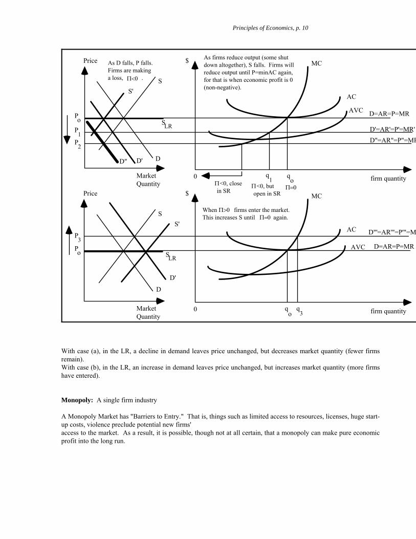
Contrasting Perfect Competition & Monopoly: Recall the law of diminishing marginal productivity: As you add more and more units of labor to a set of fixed capital, the additional output generated by each additional unit of labor declines. This is what gives MC and the other cost curves their shape. Several assumptions govern perfect competition: (i) many, many sellers and buyers, (ii) homogeneous goods, (iii) free entry and exit, (iv) perfect information & (v) factor mobility. These create a market where each firm has such a small share of the total market that they can not affect market price by changing their own price. Thus, a perfectly competitive is a "price-taker." Hence, PC firms have perfectly elastic Demand curves. Moreover, whenever D is perfectly elastic, P=MR Finally, as with any profit maximizing firm, a PC firm maximizes profits by choosing q where MR=MC. ONLY in perfect competition is this condition equivalent to finding q where P=MC. Two Cases: (a) Assume that Demand decreases. (b) Assume that Demand increases. Conclusion: A PC Market will always return to the price where P=min AC and economic profit is 0. This is the long run position of the PC market.
Principles of Economics, p. 10
S
DD'D"
Price $
Market Quantity
firm quantity
MC
AC
AVCPoP
1P
2
S
D
D'
Price $
Market Quantity
firm quantity
MC
AC
AVCPo
P3
As firms reduce output (some shut down altogether), S falls. Firms will reduce output until P=minAC again, for that is when economic profit is 0 (non-negative).
qo1
q
D'=AR'=P'=MR'D"=AR"=P"=MR
0
0
<0, but open in SR
Π <0, close in SR
ΠΠ=0
D"'=AR'"=P'"=MR
As D falls, P falls. Firms are making a loss, .Π<0
D=AR=P=MR
D=AR=P=MR
When firms enter the market. This increases S until again.
Π>0Π=0
S'
S'
q3
qo
SLR
SLR
With case (a), in the LR, a decline in demand leaves price unchanged, but decreases market quantity (fewer firms remain). With case (b), in the LR, an increase in demand leaves price unchanged, but increases market quantity (more firms have entered). Monopoly: A single firm industry A Monopoly Market has "Barriers to Entry." That is, things such as limited access to resources, licenses, huge start-up costs, violence preclude potential new firms' access to the market. As a result, it is possible, though not at all certain, that a monopoly can make pure economic profit into the long run.
Principles of Economics, p. 11
D
Market Quantity
Price
AVC
AC
MC
MR
Qo
Po
AVCo
ACo
Π>0
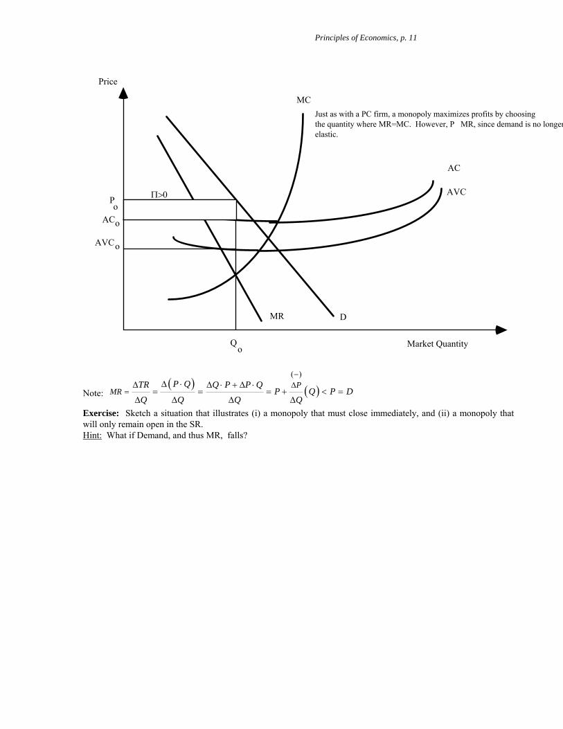
Just as with a PC firm, a monopoly maximizes profits by choosing the quantity where MR=MC. However, P MR, since demand is no longerelastic.
Note: ( ) ( )
( )P
MRP QTR Q P P Q
P Q PQ Q Q Q
−∆
=∆ ⋅∆ ∆ ⋅ + ∆ ⋅
= = = + <∆ ∆ ∆ ∆
D=
Exercise: Sketch a situation that illustrates (i) a monopoly that must close immediately, and (ii) a monopoly that will only remain open in the SR. Hint: What if Demand, and thus MR, falls?
Principles of Economics, p. 12
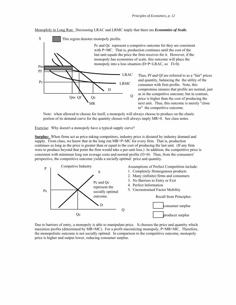
Monoploly in Long Run: Decreasing LRAC and LRMC imply that there are Economies of Scale.
D
MR
Q
$
LRAC
LRMC
Pm Pf
Pc
This region denotes monopoly profits.
Pc and Qc represent a competive outcome for they are consistent with P=MC. That is, production continues until the cost of the last unit equals the price the firm receives for it. However, if the monopoly has economies of scale, this outcome will place the monopoly into a loss situation (D=P<LRAC, so .
Π<0)
Thus, Pf and Qf are referred to as a "fair" prices and quantity, balancing the the utility of the consumer with firm profits. Note, this compromise ensures that profits are normal, just as in the competitve outcome; but in contrast, price is higher than the cost of producing the next unit. Thus, this outcome is merely "close to" the competitive outcome.
Note: when allowed to choose for itself, a monopoly will always choose to produce on the elastic portion of its demand curve for the quantity chosen will always imply MR>0. See class notes.
Qm Qf Qc
Exercise: Why doesn't a monopoly have a typical supply curve? Surplus: When firms act as price-taking competitors, industry price is dictated by industry demand and supply. From class, we know that in the long run MR=P=MC for every firm. That is, production continues as long as the price is greater than or equal to the cost of producing the last unit. (If any firm were to produce beyond that point the firm would take a per-unit loss.) In addition, the competitive price is consistent with minimum long run average costs and normal profits (Π=0). Thus, from the consumers' perspective, the competitive outcome yields a socially optimal price and quantity.
S
D
P
Q
Pc
Qc
Competive Industry
Pc and Qc represent the socially optimal outcome.
Assumptions of Perfect Competition include: 1. Completely Homogenous products 2. Many (infinite) firms and consumers 3. No Barriers to Entry or Exit 4. Perfect Information 5. Unconstrained Factor Mobility
Recall from Principles: consumer surplus producer surplus
Due to barriers of entry, a monopoly is able to manipulate price. It chooses the price and quantity which maximize profits (determined by MR=MC). For a profit maximizing monopoly, P>MR=MC. Therefore, the monopolistic outcome is not socially optimal. In comparison to the competitive outcome, monopoly price is higher and output lower, reducing consumer surplus.

Principles of Economics, p. 13
MACRO FUNDAMENTALS: OUTPUT, PRICE, EMPLOYMENT
Macro Concerns: 1. Determinants of National Income. 2. Aggregate Consumption and Investment. 3. Aggregate Price Level. Government Policy Tools: 1. Fiscal Policy (Government Expenditures). 2. Monetary Policy (Federal Reserve Bank - The Discount Rate). 3. Income-Wage Policies (Minimum wage). 4. Supply-Side Policy (Tax Cuts). Gross Domestic Product: The value of all final goods and services produced in the domestic economy in a given year. Final Goods and Services: Those that are consumed by the final purchaser. They are not used as inputs for the production of some other good or service. egg.: Automobiles, Washing Machines, Big Macs Intermediate Goods and Services: Those that are used as inputs for the production of some other good or service. egg.: Steel, Vinyl, Beef, Flour etc. Some goods may be either intermediate or final depending on use. Value Added: The difference, at each stage of the production process, between the value of product the firm sells and the cost of the materials used to produce the product. egg.: Value Added in the Production of a loaf of bread Subsets of Unemployment: 1. Frictional Unemployment: Reflects skill or job matching problems that individuals may face at any
time. Natural Rate of Unemployment: It's around 5-6%. It represents those workers that are in transition or between jobs. The life-cycle and the business cycle make this inevitable. People move in and out of jobs because of illness, failing businesses, school etc.. N.R.U. ≈FR.U.
2. Structural Unemployment: Arises from economic transition. For example automation forced people
to find other jobs. Blue collar jobs decreased in number, but the service sector expanded. It takes time for the work force to shift to match a newly defined economy.
3. Cyclical Unemployment: The increase in unemployment due to downward trends in the business
cycle or recession. Cyclical = Actual - Natural Rate. Seasonal Unemployment: Expected variations in job opportunities due to seasonally dependent jobs.
Points to note:
Discouraged workers and/or homeless are not included in these figures. Recessions can hurt the economy in the long run as well because during a recession there is not
as much investment. However, recessions are also seen to have a cleansing effect as firms act to eliminate their less efficient resources. Recessions are also linked to reduced inflation.
There are large discrepancies in the unemployment rate across demographic groups at different times.
Unemployment is seen as a destabilizing economic and political phenomenon.

Principles of Economics, p. 14
GDP or Aggregate Expenditures (Y): The total value of all final goods and services produced in a given year.
PRICE INDICIES: REAL VS. NOMINAL Real Values: Values of goods and services expressed in terms of a base year. Nominal Values: Values of goods and services expressed in today’s' dollars. Inflation And Price Indices Inflation is the percentage increase in the overall price level. It can be sustained over a period of time or be a short term phenomenon. When calculating price indices we wish to measure inflation so we fix a bundle of goods and compare the cost of this bundle at different periods in time. Essentially, the bundle is fixed as prices vary. Consumer price index: The CPI includes price changes for a sample bundle of consumer goods. Quantities are fixed as prices vary. Calculated monthly by the Bureau of Labor Statistics. Producer Price Index: The PPI includes price changes for a sample bundle of producer goods. The CPI overestimates changes in the cost of living because of: • Substitution effects: People tend to substitute from goods that become relatively more expensive.
They will not purchase the same quantities. Thus, expenditures may only rise slightly compared to the CPI.
• Arrival of new goods, Disappearance of old ones: Compact discs and PC's will not be in a base year before 1982 or so.
• Quality Improvements: The CPI ignores improvements in quality. Example: Calculating the CPI. Bread Milk Cotton (bale) Consumption 3 5 1 1979 $ 0.60 1.50 5.00 1986 $ 0.80 up 33% 1.90 up 26.7% 6.00 up 20% 1993 $ 1.00 up 25%,66.7% 2.20 up 15.8%,46.7% 7.50 up 25%,50% Price Index: We use 1979 as the base year.
Thus, PI1979 = Bundle Price in 1979 $ Base Year Bundle Price
= 14. 3014. 30
= 1.00 or 100%.
PI1986 = Bundle Price in 1986 $ Base Year Bundle Price
= 17. 9014. 30
= 1.252 or 125.2%.
PI1993 = Bundle Price in 1993 $ Base Year Bundle Price
= 21. 5014. 30
= 1.504 or 150.4%.
Inflation = The percentage change in price indices.
Inflation between 1979 and 1986: 125 . 2 − 100
100 = 0.252 or 25.2%.

Principles of Economics, p. 15
Inflation between 1979 and 1993: 150 . 4 − 100
100 = 0.504 or 50.4%.
Inflation between 1986 and 1993: 150 . 4 − 125 . 2
125 . 2 = 0.201 or 20.1%.
Example: If, in 1986, the minimum wage and the CPI were $3.35 and 1.252 and, in 1993, the minimum wage and the CPI were $4.25 and 1.504, in which year were people better off? What if the minimum wage for 1993 was only $4.00?
Solution: a. RW 85 = 3 . 35
1 . 252 = 2 . 68 . RW 93
1 = 4 . 25
1 . 504 = 2 . 83 .
b. RW 932 =
4 . 001 . 504
= 2 . 66 .
Note: Inflation rates do not depend upon choice of base year.
MODELING THE MACRO ECONOMY Aggregate (General) Price Level: CPI, GDP Deflator An increase (decrease) in this aggregate price level is INFLATION (deflation). Can be thought of as the average "cost of living". Aggregate Output: GDP. ECONOMIC GROWTH: The rate at which output is increasing/the economy is expanding. Aggregate Demand: The relationship between the general price level and the quantity of aggregate output demanded. It is represented by a downward sloping curve (due to the aggregate effect of the Law of Demand). Aggregate Supply: The relationship between the general price level and the quantity of aggregate output supplied. It is represented by an upward sloping curve (due to the aggregate effect of the Law of Supply). CAUTION! In Micro a change in the price of a single good leads to changes in the demand or supply for related goods (sub. & inc. effects). In the aggregate, an increase in the general price level means that the prices of all goods (on average) have increased.

Principles of Economics, p. 16
THE GOODS MARKET, AGGREGATE DEMAND AND SUPPLY
Aggregate Demand:
AD
Price Level
Total Output
P
Q AD is negatively sloped because: (change in output demanded) 1. Wealth Effect: A higher price level reduces purchasing power of existing wealth 2. Foreign sector substitution effect: As US prices rise, foreigners will purchase (cheaper) goods made elsewhere. In addition, firms may decide to locate in countries where prices and costs are lower. This hurts investment. 3. Interest rate effect: Borrowing need to finance any given project increases. This increases the demand for loanable funds, and thus, the rate of interest. Things that SHIFT AD: (At any given price level, aggregate demand changes) 1. Consumption: i. Changes in Disposable Income (taxes etc.) ii. Changes in wealth or expected income (lottery). iii. Demographics (size and age of average household). iv. Household indebtedness. v. Expectations. 2. Investment: i. Expected rates of return on investment. ii. Cost of capital. 3. Government: i. Government purchases ii. Tax rates iii. Money (short-run phenomenon). 4. Foreign Sector: (X-M) = net exports i. Exports ii. Imports: All previous categories also affect imports. Important: These together yield total (aggregate) expenditures.

Principles of Economics, p. 17
Aggregate Supply
AS
Price Level
Total Output
P
Q
Classical Portion
Keynesian portion
Classical portion: AE = Y and S = I always! Plus, even if it didn't, interest rate, prices and wages will adjust so that full-employment always exists. Thus, AS vertical and an increase in AD translates into higher prices only! Keynesian portion: Unemployment DOES exist! Wages and prices are (downwardly) sticky. S and I are not necessarily equal. Thus, AD determines output AS is upward sloping because: (change in output supplied) 1. Stickiness: Prices adjust faster than production costs. 2. Capacity: it is more difficult to press idle resources into action when the economy is near capacity. 3. Diminishing returns: As output grows, eventually diminishing returns are reached. That is, additional workers, capital are less efficient than those hired previously. This puts upward pressure on prices as firms try to cover the increase in costs resulting from the drop in average productivity. Shifts in AS: (at any given price level, firms change output supplied) 1. Resource Costs 2. Technology 3. Expectations (expected inflation, prosperity) 4. Government Policies (Payroll, corporate taxes; Welfare and work vs. leisure decisions; Research funding and protection)

Principles of Economics, p. 18
Putting it together... Self Regulating Macroeconomic Equilibrium: INVENTORY CHANGES ALERT FIRMS! When AD and AS are equal there is no excess demand or supply of goods and services in the economy.
Price
Y
AS
1 AD
Y o
P o
Example 1: Describe the effect on prices and output when there is an increase in taxes and a serious natural disaster. Solution: The effect on the price level is ambiguous, but Y falls unambiguously.
ASP
Y
AS1
2
AD1 AD 2
?
Example 2: Expectations and Inflation Assume the cost of oil increases. This will tend to shift the AS to the left, raising prices and lowering output. If the government wishes to restore output to its previous level then it must pursue expansionary policies. This will increase AD, restoring output to its previous level, but increasing prices more!!!!!!

Principles of Economics, p. 19
P
Y
AD2 AD1
AS2 AS1
a
b c
An inflationary (expansionary) gap occurs when SR output exceeds LR capacity. This increases the costs firms face, thus increasing prices. In this case the actual rate of unemployment is lower than the natural rate of unemployment! As a result, wages rise, causing the AS to shift to the left, to a new equilibrium at a higher price level, but at the natural output level.
Price
Y
P o
LRAS
Y N
1 AD
AD2
Expansionary Gapor Inflationary Gap
Y o
1 ASAS2
A recessionary gap occurs when SR output is less than LR capacity. In this case the actual rate of unemployment is higher than the natural rate of unemployment! As a result, wages fall via lay-offs and wage reductions, causing the AS to shift to the right, to a new equilibrium at a lower price level, but at the natural output level. Note: we are inside the PPF!

Principles of Economics, p. 20
Price
Y
LRAS
Y N
1 AD
AD2 Y o
P o
Recessionary GapAS2
AS1
MONETARY SECTOR
Money Demand: The amount of money held as cash or in non-interest bearing checking accounts. Interest: The amount paid for the use of someone else's money. Interest rate: The opportunity cost of holding money. Motives for Holding Money: 1. Transactions Motive: In order to purchase goods and services. 2. Speculative Motive: At times people hold money in order to maximize one's return on an investment. 3. Precautionary Motive: In order to guard against the unknown, to provide short term security. Optimal Balance: If Joe Moneypenny earns $2000 a month then if he draws on that all month his average monthly balance is considered to be $1000. If he chooses to purchase a bond with half of the salary, selling it at mid-month, then his average monthly balances would be $500. etc.. Obviously average monthly balances will ultimately depend, at least in part, on the rate of interest. It might seem that, in order to maximize the return from interest, one would hold as little money as possible. However, in practice there are transaction costs associated with making exchanges: ATM fees, brokerage fees, time costs etc..
0.5 1 1.5 2
Demand for $
0 Time (months)
2000
1000
500
Average
Average

Principles of Economics, p. 21
Law of Interest: When interest rates are high people will hold less money than when interest rates are low because when r is high, the opportunity cost of holding money is high. Money Demand Curve: r = rate of interest. M = quantity of money held within a given interval of time.
r
M
Md
The Bond Market: T-Bills: Government securities with maturity dates of less than one year. Bonds: Government securities with maturity dates of equal to or more than one year.
S
D B
B
B
B P
The secondary market for bonds: As the interest rate increases the price of bonds decreases and vice versa. Example: Assume that one buys a $100 U.S. bond which yields a fixed coupon payment of $10 (10%) until maturity. If interest rates fall to 5%, then someone would be willing to pay up to $104.76 for that bond (they will receive $110 which is 105% of $104.76). If interest rates rise to 15% then someone will be willing to pay at most $95.65 (then $110 represents a 15% return).
Principles of Economics, p. 22
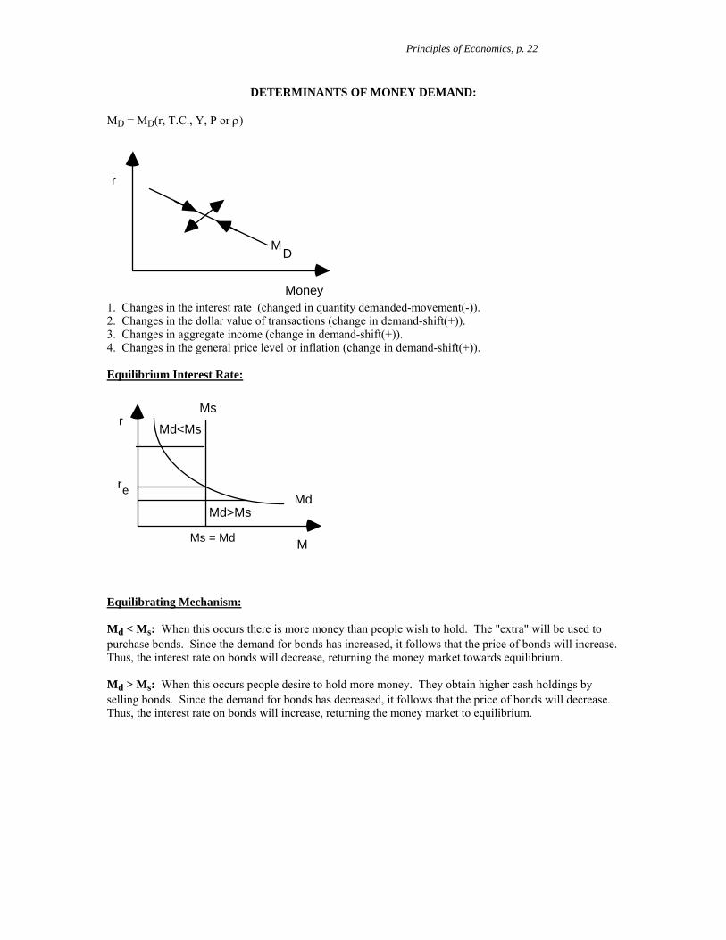
DETERMINANTS OF MONEY DEMAND: MD = MD(r, T.C., Y, P or ρ)
r
D M
Money 1. Changes in the interest rate (changed in quantity demanded-movement(-)). 2. Changes in the dollar value of transactions (change in demand-shift(+)). 3. Changes in aggregate income (change in demand-shift(+)). 4. Changes in the general price level or inflation (change in demand-shift(+)). Equilibrium Interest Rate:
r
M
Md
Ms
Ms = Md
Md>Ms
Md<Ms
r e
Equilibrating Mechanism: Md < Ms: When this occurs there is more money than people wish to hold. The "extra" will be used to purchase bonds. Since the demand for bonds has increased, it follows that the price of bonds will increase. Thus, the interest rate on bonds will decrease, returning the money market towards equilibrium. Md > Ms: When this occurs people desire to hold more money. They obtain higher cash holdings by selling bonds. Since the demand for bonds has decreased, it follows that the price of bonds will decrease. Thus, the interest rate on bonds will increase, returning the money market to equilibrium.
Principles of Economics, p. 23
Policy Tools: The Fed can act to try to control the rate of interest by altering the money supply. For example, if Ms increases then, temporarily, at the current rate of interest, there is an excess supply of money. The bond market will then adjust to bring the interest rate down. • Monetary Policy is said to be tight if the Fed acts to contract the money supply or slow its rate of
growth. • Monetary Policy is said to be loose or easy if the Fed acts to increase the money supply or increase its
rate of growth. The Money Supply and the Federal Reserve February 20, 2006 Definitions of Money: 1. Medium of Exchange - effectiveness relies on general acceptance as legal tender. - very liquid. - superior to barter system: doesn't require coincidence of wants. 2. Store of Value - can be used to transfer purchasing power to another period. - note that there is an opportunity cost associated with holding cash as opposed to some appreciable asset. 3. Unit of Account - provides a consistent way of measuring prices. Types of Monies: 1. Commodity Monies: Have intrinsic value e.g. gold, silver, diamonds. 2. Fiat Monies: No intrinsic value, relies on acceptance. Currency Debasement: Erosion of real value of the currency because of inflation.

Principles of Economics, p. 24
Measuring Money: M1, M2, M3, etc.
Billions of $
200
800
3000
3800
M1 M2 M3
Currency
Checking deposits
Savings, Money mkt., deposits. Small C.D.'s. Overnight rep. agree.
M1
M2
Large C.D.'s
Principles of Economics, p. 25
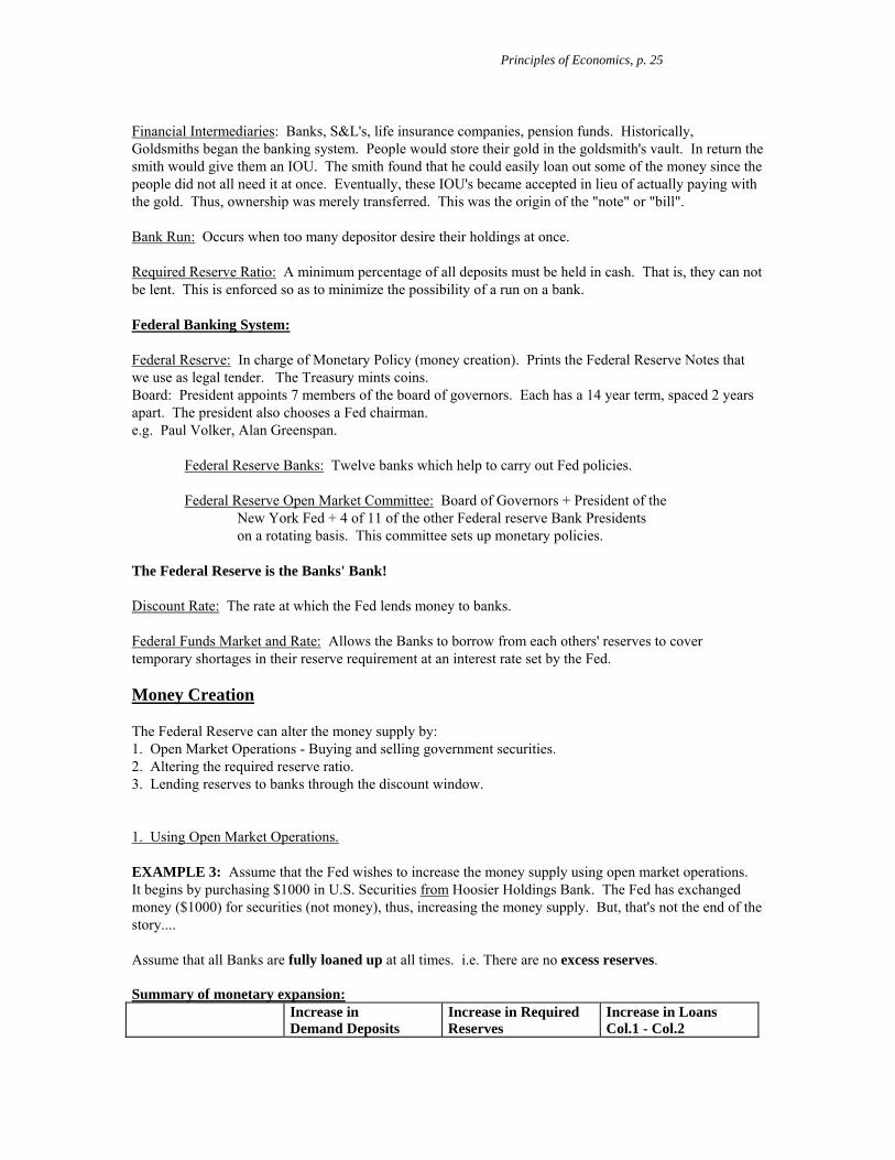
Financial Intermediaries: Banks, S&L's, life insurance companies, pension funds. Historically, Goldsmiths began the banking system. People would store their gold in the goldsmith's vault. In return the smith would give them an IOU. The smith found that he could easily loan out some of the money since the people did not all need it at once. Eventually, these IOU's became accepted in lieu of actually paying with the gold. Thus, ownership was merely transferred. This was the origin of the "note" or "bill". Bank Run: Occurs when too many depositor desire their holdings at once. Required Reserve Ratio: A minimum percentage of all deposits must be held in cash. That is, they can not be lent. This is enforced so as to minimize the possibility of a run on a bank. Federal Banking System: Federal Reserve: In charge of Monetary Policy (money creation). Prints the Federal Reserve Notes that we use as legal tender. The Treasury mints coins. Board: President appoints 7 members of the board of governors. Each has a 14 year term, spaced 2 years apart. The president also chooses a Fed chairman. e.g. Paul Volker, Alan Greenspan. Federal Reserve Banks: Twelve banks which help to carry out Fed policies. Federal Reserve Open Market Committee: Board of Governors + President of the New York Fed + 4 of 11 of the other Federal reserve Bank Presidents on a rotating basis. This committee sets up monetary policies. The Federal Reserve is the Banks' Bank! Discount Rate: The rate at which the Fed lends money to banks. Federal Funds Market and Rate: Allows the Banks to borrow from each others' reserves to cover temporary shortages in their reserve requirement at an interest rate set by the Fed. Money Creation The Federal Reserve can alter the money supply by: 1. Open Market Operations - Buying and selling government securities. 2. Altering the required reserve ratio. 3. Lending reserves to banks through the discount window. 1. Using Open Market Operations. EXAMPLE 3: Assume that the Fed wishes to increase the money supply using open market operations. It begins by purchasing $1000 in U.S. Securities from Hoosier Holdings Bank. The Fed has exchanged money ($1000) for securities (not money), thus, increasing the money supply. But, that's not the end of the story.... Assume that all Banks are fully loaned up at all times. i.e. There are no excess reserves. Summary of monetary expansion: Increase in
Demand Deposits Increase in Required Reserves
Increase in Loans Col.1 - Col.2

Principles of Economics, p. 26
I.U.'s Bank 1,000 100 900 Honest Karl's Bank 900 90 810 Rebecca's Bank 810 81 729 Gertrude's Bank 729 72.90 656.10 All Other Banks 6,561 656.10 5,904.90 Total 10,000 1,000 9,000
Thus, The actual money supply has increased by 1 − RRR ( ) k ∆ sec urities ( ) = ∆ sec urities RRR k = 1
∞ ∑ .
∴ The Money Multiplier = 1
RRR .
Question: How does this scenario change if the RRR increases? Decreases? If the Banks are not necessarily fully loaned up? EXAMPLE 1: If the Fed sells $5000 in government securities via OMO with a RRR of 25%, by how much will the money supply change? SOLUTION: It will DECREASE by $5,000(1/0.25) = $20,000. 2. Changing the Required Reserve Ratio: This allows for greater growth in the money supply if the RRR is lower, and less growth in the money supply if the RRR is raised. EXAMPLE 2: If the Fed changes the RRR from 20% to 10%, by how much will the money supply change? What if it increases the RRR to 25%? SOLUTION: It will INCREASE by the ratio between the new multiplier and the old: 1/0.2 = 5, 1/0.1 = 10, thus 10/5 =2, and the money supply will double.
If the RRR increases to 25% then the money supply will DECREASE to
1 0 . 25
1 0 . 20
= 4 5
= 0 . 80 or
80% of its previous size. 3. Using the Discount Window: Since the Fed prints the money, the money it lends is new. Lending it to banks will have the same multiplier effect on the size of the money supply. However, it is difficult to use this method to regulate the money supply since it relies on the timing, wishes and whims of the Banks that require loans. Plus, changing the discount rate will never increase the money supply! It can only affect how much it will decrease because the net effect of the principle is zero. The interest is money removed from the economy. EXAMPLE 3: If the Fed loans $5000 to a bank and the discount rate is 10%, by how much will the money supply change? SOLUTION: It will DECREASE by $5,000(0.10) = $500. The Money Supply Curve is assumed to be independent of the interest rate (price of money), thus it is perfectly inelastic.

Intermediate Microeconomics Study Guide SECTION 1 Part I: Provide concise definitions. Usually an appropriate, well-labeled graph or mathematical relation is sufficient. (2 points each) 1. Marginal Utility: 4. Marginal Rate of Substitution: 2. Substitution Effect: 5. Income Effect: 3. Indifference Curve: 6. Consumer Equilibrium: Part II: Make your answers clear, concise, and comprehensive. Usually an appropriate, well-labeled graph with a one or two sentence explanation is sufficient. Begin each problem (1, 2, 3,...etc.) on a new page. (4 points each for parts i, ii, iii, etc.) 1. i. Katherine has a budget of $180 for shoes and hats. If shoes cost $30 and hats cost $20 each, describe and sketch and thoroughly label her budget constraint. As usual, assume (infinite) divisibility of goods. ii. Repeat part (i) if the price of hats increases to $30 a pair. iii. Repeat part (i) if her budget decreases to $120. iv. Repeat part (i) if the store restricts hat purchases to three per customer. 2. i. Provide a scenario (example) of an economic good that is a "bad." Pick a good that can be compared to your "bad." Sketch a representation of the indifference curves (map). ii. Do these indifference curves follow the law of diminishing marginal rate of substitution? Explain. 3. Let y be a normal good and let x be an inferior good. i. Sketch the income consumption curve (ICC), complete with a representative (likely) set of preferences (indifference curves /map). ii. Sketch a representative Engel Curve for x. Part III: Make your answers clear, concise, and comprehensive. Usually an appropriate, well-labeled graph with a one or two sentence explanation is sufficient. Begin each problem (1, 2, 3,...etc.) on a new page. (5 points each for parts i, ii, iii, etc.) 1. Given goods x and y, sketch the indifference curve for u 16o= when:
i. ( )u x, y x y= + . ii. u x,y( ) = 2x + y . iii. u x,y( ) = min{2x, y}. iv, v, and vi. Next, given the budget constraint, 3x + y = 30, explicitly determine the optimal bundles for each utility function in parts i, ii, and iii. Note, you may find it expedient to do i & iv together, and so on. 2. i. Regarding cell phone usage, sketch the budget constraint under (a) a pay as you go plan and (b) a plan in which you pay a flat fee, t, for free minutes, then a per unit fee for every minute thereafter. oxii. Sketch the preferences an individual must have in order to suffer a loss in utility under plan b. iii. Regarding school choice, assuming a public school tax equal to t, sketch the budget constraint when (a) there is also a private school choice for a minimum additional payment equal to t and (b) when there exist private school vouchers. iv. Sketch the preferences an individual must have if they choose the public school option before and after the voucher system is implemented. 3. Given income, M, and goods, x and y, illustrate the substitution and income effects after the price of x falls when preferences are: i. Cobb-Douglas ('typical'). ii. Leontief (perfect complements).

Econ155,TH1, page 2
SECTION 1 SOLUTIONS
1. Marginal Utility = ∆TU∆x
2. Substitution Effect: A change in consumption of good x due to a change in the relative price of good x. 3. Indifference Curve: A set of consumption bundles all yielding the same utility.
4. MRS = MU xMUy
. Demonstrates the trade-off that maintains constant utility; it is the slope of the
indifference curve. 5. Income effect: A change in consumption of good x due to a change in real purchasing power.
6. Consumer equilibrium: MUx
Px=
MUyPy
.
Part II:
hats
shoes
96
MPy
=6
MPx
iii
4 iii
3
iv
1.
2.
i.garbage
food
u0 u1 u2 u3 u 4
ii. In this case the marginal rate of substitution reflects not a trade-off, but a bribe. The indifference curves have positive slope. MUg < 0. MUg ↑ since the marginal disutility of garbage increases as the amount of
garbage increases. As food consumption increases, . Thus, MUf ↓ MRS =MU f
MUg↓ .
Econ155,TH1, page 3
y
x
u2
u1
uo
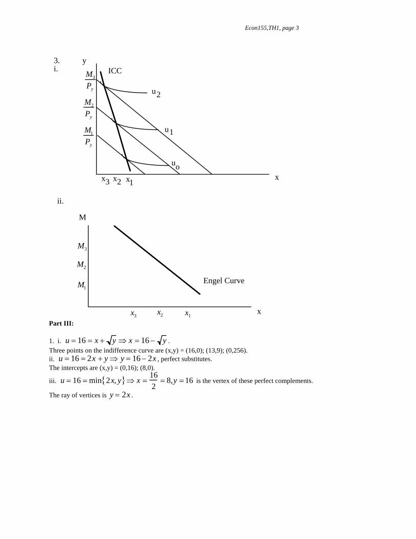
3. i. ICC
x1x2x3
M1
Py
M2
Py
M3
Py
M
x
Engel Curve
ii.
M1
M2
M3
x1x2x3 Part III: 1. i. u = 16 = x + y ⇒ x = 16 − y . Three points on the indifference curve are (x,y) = (16,0); (13,9); (0,256). ii. u = 16 = 2x + y ⇒ y = 16 − 2x , perfect substitutes. The intercepts are (x,y) = (0,16); (8,0).
iii. u = 16 = min 2x, y{ }⇒ x =162
= 8,y = 16 is the vertex of these perfect complements.
The ray of vertices is . y = 2x

Econ155,TH1, page 4
y
x16
256
i.
u=16
y
x
16
ii.
8
u=16
y
x
16
8
y=2x
u=16
iii.
iv. L = x + y + λ 30 − 3x − y( ). ∂L∂x
=1 − 3λ ⇒ λ =13
.
∂L∂y
=12
y− 1
2 − λ ⇒ y =1
4λ2 =94
= 2.25 . 30 = 3x + 2.25 ⇒ x = 9.25 .
v. u = 2x + y ⇒ y = u − 2x ⇒ slope = −2 . Budget Constraint: y = 30 − 3x ⇒ slope = −3 . The BC is steeper. Optimal bundle is y=30, x=0. vi. y = 2x, y = 30 − 3x ⇒ (x, y) = (6,12) .

Econ155,TH1, page 5
other goods
cell phone usea b
xo
ua
ub
2. i. & ii.
Let prefs. reflect a bias towards other goods.
MPog
− t
2.
Let prefs. reflect a bias towards other goods.
other goods
a beducation
MPog
− t
epub
MPog
− 2t
iii. &iv.
uo
u1
y
x
u1
uo
sub inc
3. i.

Econ155,TH1, page 6
y
x
u1
uo
3. ii.
inc
only an income effect.
There exists
SECTION 2
INTERTEMPORAL ALLOCATION
1. Let preferences over current and future consumption be defined by u(C1,C2) = lnC1 + C2 . Let the interest rate between periods be 10%. Assume current income is $40,000 and future income is $50,000. i. What is the present value of future income? ii. Find the optimal allocation of current and future consumption. Is this individual relatively patient or impatient? 2. Assume the interest rate increases from 10% to 20%. i. On two separate graphs, illustrate preferences that indicate (a) a rise in utility after the rate increase, and (b) a fall in utility after the rate increase. ii. Explain the intuition justifying the outcomes in (i.a.) & (i.b.). Hint: Look at possibly dominant income or substitution effects. 3. Use the results from our intertemporal model to explain why, when compared to graduate students in other fields, graduate students in law tend to drive nicer cars despite being the same age and having comparable economic status. 4. Using the two-period intertemporal model, describe the indifference curves of an individual who believes that Armageddon is to come in period two!
LABOR/LEISURE
1. The year is 2015 and your little neighbor Tommy would like to go to Holy Cross to study English. Unfortunately, Tommy also likes to watch TV. Left to his own devises, he would forego studying completely and spend all his discretionary time (up to 60 hours per week) watching TV! After complaining incessantly to you, Tommy's parents let slip that the little guy receives $100 a week in allowance. Recalling a rather enlightening microeconomics course you once had at the Cross, you advise Tommy's parents to eliminate the 'free' allowance. Instead, you tell them to pay Tommy $20 for every hour he studies. i. Use consumer choice theory to describe the effect of tying Tommy's allowance to his study time. Under typical preferences would you expect Tommy's study time to increase? Justify with a sketch. Hint: Sketch the relevant budget constraint and indifference curves, comparing optimal bundles of TV time and allowance before and after you change the allowance policy.

Econ155,TH1, page 7
ii. Under what conditions (preferences) will your suggestion not work? That is, is it possible that, despite your suggestion, Tommy could still devote all 60 hours to watching TV? Be explicit and illustrate graphically. 2. Assume that you have 60 hours per week to either work or use for leisure time. Also assume that your hourly wage is $20. The budget line for this scenario follows. Incorporate the graph into your analysis. Note that the slope of the line is -w, where w is the hourly wage.
u o
Leisure time per week (hrs.)60
$, OG
$1200
i. Describe the effects on the budget constraint and utility if your hourly wage increases to $25.

Econ155,TH1, page 8
ii. When ones wage increases there is incentive to work more (because your time is more valuable now) and to allow for more leisure time (because leisure is a normal good). When the wage increase leads to more working hours we say that the substitution effect dominates. Why? When the wage increase leads to more leisure (fewer hours spent working) we say that the income effect dominates. Why? iii. Sketch two sets of preferences (indifference curves). One must illustrate a dominant substitution effect and the other, a dominant income effect. iv. Referring to the original graph again, what is the effect on the budget line and potential effect on utility and leisure time if, at an hourly wage of $20, you now make "time and a half" after 40 hours ($30 per hour for each hour after 40). 3. Assume that you have 60 hours per week to either work or use for leisure time. Also assume that your hourly wage is $20. The budget line for this scenario follows. Incorporate figure 2 into your analysis. Note that the slope of the line is -w, where w is the hourly wage.
u o
Leisure time per week (hrs.)60
$, OG
$1200 figure 2
i. Describe the effects on the budget constraint and utility if your hourly wage increases first to $25 and then to $30. ii. Based on your answer to (i), sketch the labor supply curve. iii. Does your labor supply curve illustrate a dominant income or substitution effect? Explain! iv. If necessary, amend your answer to (i) to generate a backward bending labor supply curve. Illustrate and explain.
CONSUMER OPTIMA Note, in the problems that follow use the method of LaGrange Multipliers to obtain the optimal bundles. Feel free to use Maple V.5. 1. i. Given u(x, y) x y= + px = 4 and py = 5, sketch the income-offer curve and Engel curve after determining the optimal bundles when m = 200, 300 & 400. ii. Can you find the equation for the Engel curve with this information? 2. Given with m = 200 and py = 5, sketch the price-offer curve for good x after determining the optimal bundles when px = 4, 3 and 2.
( ) 0.75 0.25u x, y x y=
3. Find the demand function for x when py =5 and m = 200, assuming that preferences are given by
. ( ) 0.75 0.25u x, y x y= 4. Given the preferences defined in (3), derive the value function. Assuming m= 100, px = 2 and py = 5, calculate the consumer's maximum utility.

Econ155,TH1, page 9
5. i. In what manner is Pareto Optimality efficient? ii. On the graph below explicitly demonstrate how point p could be Pareto optimal when starting from an allocation w. "Spam" is considered a normal good - not that it matters here.
0
0'
Jeff
Dan
Spam
Ji
D j
.p
. w
Corn Dogs
PRINCIPLES OF PRODUCTION 1. (4 points) The following illustrates short run costs. Complete the table. Output 0 1 2 3 4 5 6 TC 24 108 MC - 16 52 TFC TVC 50 AC(ATC) - 47 AVC - 39.2 AFC - 2. Determine whether the following statements are true or false. You MUST explain your reasoning! i. Other things being constant, if the fixed costs of a firm were to increase by $100,000 per year, AFC and ATC would rise, but MC would remain unchanged. ii. A typical firm's average total cost (ATC) must fall with expansion of output if its marginal cost per unit is below it and falling. iii. Economies of scale (IRS) exist over the range of output for which the long-run average cost curve is falling. iv. At 10 units of output, a firm's U-shaped marginal cost and average total cost curves each equal $1000. Therefore, at 11 units of output its marginal cost is less than $1000 and its average total cost is greater than $1000. 3. What primarily distinguishes our new production model from that learned in principles?
PRODUCTION THEORY
1. For each of the following production functions: (a) explicitly determine whether increasing, decreasing or constant returns to scale exist. (b) illustrate (a) by sketching three appropriately chosen (and labeled) isoquants. i. F L, K( ) = LK ii. F L , K( ) = 2L + 5K iii. F L , K( ) = min 2L, 5K{ } iv. F L , K( ) = L + ln K( )
Econ155,TH1, page 10
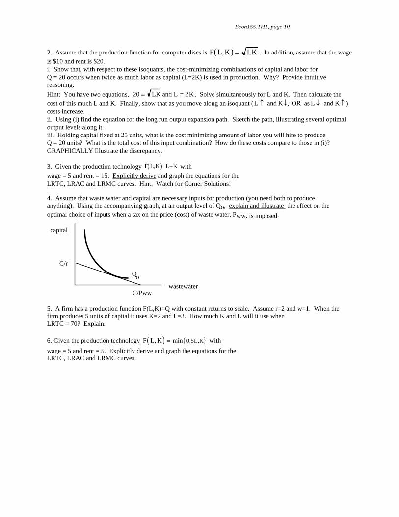
2. Assume that the production function for computer discs is F L,K( ) = LK . In addition, assume that the wage is $10 and rent is $20. i. Show that, with respect to these isoquants, the cost-minimizing combinations of capital and labor for Q = 20 occurs when twice as much labor as capital (L=2K) is used in production. Why? Provide intuitive reasoning. Hint: You have two equations, 20 = LK and L = 2K . Solve simultaneously for L and K. Then calculate the cost of this much L and K. Finally, show that as you move along an isoquant (L ) costs increase.
↑ and K↓, OR as L ↓ and K ↑
ii. Using (i) find the equation for the long run output expansion path. Sketch the path, illustrating several optimal output levels along it. iii. Holding capital fixed at 25 units, what is the cost minimizing amount of labor you will hire to produce Q = 20 units? What is the total cost of this input combination? How do these costs compare to those in (i)? GRAPHICALLY Illustrate the discrepancy. 3. Given the production technology ( )F L,K L K= + with wage = 5 and rent = 15. Explicitly derive and graph the equations for the LRTC, LRAC and LRMC curves. Hint: Watch for Corner Solutions! 4. Assume that waste water and capital are necessary inputs for production (you need both to produce anything). Using the accompanying graph, at an output level of Qo, explain and illustrate the effect on the optimal choice of inputs when a tax on the price (cost) of waste water, Pww, is imposed.
wastewater
C/r
C/Pww
capital
Qo
5. A firm has a production function F(L,K)=Q with constant returns to scale. Assume r=2 and w=1. When the firm produces 5 units of capital it uses K=2 and L=3. How much K and L will it use when LRTC = 70? Explain. 6. Given the production technology ( ) {0.5L,KF L, K min= } with wage = 5 and rent = 5. Explicitly derive and graph the equations for the LRTC, LRAC and LRMC curves.
Econ155,TH1, page 11
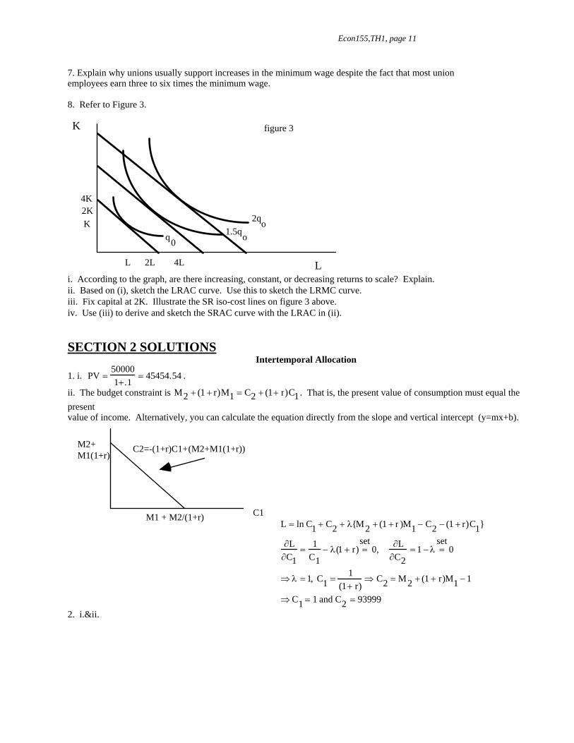
7. Explain why unions usually support increases in the minimum wage despite the fact that most union employees earn three to six times the minimum wage. 8. Refer to Figure 3.
L
K
o1.5q2qo
q0
L 2L 4L
K2K4K
figure 3
i. According to the graph, are there increasing, constant, or decreasing returns to scale? Explain. ii. Based on (i), sketch the LRAC curve. Use this to sketch the LRMC curve. iii. Fix capital at 2K. Illustrate the SR iso-cost lines on figure 3 above. iv. Use (iii) to derive and sketch the SRAC curve with the LRAC in (ii). SECTION 2 SOLUTIONS
Intertemporal Allocation
1. i. PV =500001+.1
= 45454.54 .
ii. The budget constraint is M2 + (1 + r)M1 = C2 + (1+ r)C1. That is, the present value of consumption must equal the present value of income. Alternatively, you can calculate the equation directly from the slope and vertical intercept (y=mx+b).
C2=-(1+r)C1+M2+ M1(1+r)
M1 + M2/(1+r) C1
(M2+M1(1+r))
L = ln C1 + C2 + λ{M2 + (1 + r )M1 − C2 − (1 + r)C1}
∂L∂C1
= 1C1
− λ(1 + r) =set
0, ∂L∂C2
= 1 − λ =set
0
⇒ λ = 1, C1 = 1(1+ r)
⇒ C2 = M2 + (1 + r)M1 − 1
⇒ C1 = 1 and C2 = 939992. i.&ii.

Econ155,TH1, page 12
C2
C1
slope=-1.1
slope=-1.2C2
C1
slope=-1.1
slope=-1.2 uou1
uo
u1
When patient, it is more likely that the increase in r will improve utility.
When impatient, it is more likely that the increase in r will reduce utility.
When patient, the individual is much more likely to benefit from the opportunity to substitute present consumption for future consumption. 3. Law students spend fewer years in graduate school and generally expect they have a higher present value of future income. Thus, they are more likely to tolerate a greater amount of debt. 4. In this case, the individual does not believe that there will be a period 2! Thus, he will consume everything in period one.
C2
C1
uo u1 u2 u3 u4The indifference curves arevertical! Providing more consumption in period 2 will not alter his utility.
Econ155,TH1, page 13
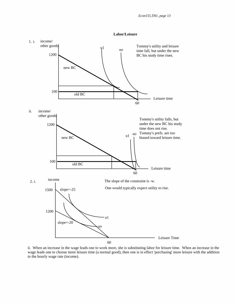
Labor/Leisure
income/ other goods
Leisure time60
1200
100
uou1
new BC
old BC
Tommy's utility and leisure time fall, but under the new BC his study time rises.
i.1.
income/ other goods
Leisure time60
1200
100
uou1new BC
old BC
Tommy's utility falls, but under the new BC his study time does not rise. Tommy's prefs. are too biased toward leisure time.
ii.
Leisure Time
income The slope of the constraint is -w.
slope=-20
slope=-25
60
1200
1500
2. i.
uo
u1
One would typically expect utility to rise.
ii. When an increase in the wage leads one to work more, she is substituting labor for leisure time. When an increase in the wage leads one to choose more leisure time (a normal good), then one is in effect 'purchasing' more leisure with the addition to the hourly wage rate (income).

Econ155,TH1, page 14
2. iii.
uo
u1
u1'
Leisure Time
income
60
1200
1500 Note that u1 describes a dominant substitution effect, whereas u1' describes a dominant income effect. Warning, u1 and u1' cannot coexist! They represent mutually exclusive alternatives.
l1 lo l1'
uou1
Leisure Time
income
60
1200
1500
20
2. iv.
Leisure Time
income
60
1200
1500
20
slope=-20
slope=-30
With time and one half, the individual may choose to work more, as indicated.
14001400
3. i. - iv.
uo
u1
Leisure Time
income
60
1200
1500
l1 l2 lo
u2
wage
Labor
SL
lo l2 l120
25
30
w=20
w=25
w=30
Since labor falls with wage, there is a dominant income effect.
When labor increases with the wage there is a dominant substitution effect.

Econ155,TH1, page 15
Consumer Optima y
x50 75 100
40
60
80
uo
u1
u2
ICC M
x
1. i.
x1
x2x 3x
1x2x 3
Engel Curve
ii. L = x + y + λ{M − Pxx − Pyy} . So, ∂L∂x
=12
x−1/ 2 − λPx =set
0, ∂L∂y
= 1− λPy =set
0,
⇒ λ =1
Py, x =
Py2P x
⎛
⎝ ⎜
⎞
⎠ ⎟
2. Using the BC, M = Px
P y2Px
⎛
⎝ ⎜
⎞
⎠ ⎟
2+ Pyy. Thus, y =
MP y
−P y4P x
. View the optimum as equations
of x and M, and of y and M. Therefore, the Engel curve for x is constant (vertical) since changes in M do not affect x
x =Py
2Px
⎛
⎝ ⎜
⎞
⎠ ⎟
2⎛
⎝
⎜ ⎜
⎞
⎠
⎟ ⎟ .
The Engel curve for y is linear, with a positive slope M = Pyy +P y
2
4Px
⎛
⎝
⎜ ⎜
⎞
⎠
⎟ ⎟
. The Engel curve for y is sketched below.
M
y
P2y
4 Px
2. Using the Maple worksheet from Take Home Test 1 (or use #3 below), if Px = 4, then y =10, x= 37.5 and λ = .1347. If Px = 3, then y =10, x= 50 and λ = .1672. If Px = 2, then y =10, x= 75 and λ = .2266. Thus, the price offer (cons.) curve is horizontal.
y
x50 66.67 75 100
10
37.5
PCC

Econ155,TH1, page 16
3. L = x.75y.25 + λ{200 − Pxx − 5y}
∂L∂x
=.75x−. 25y.25 − λP x =set
0, ∂L∂y
=.25x. 75y−.75 − 5λ =set
0
⇒ y = xPx15
⎛ ⎜
⎞ ⎟ .
⎝ ⎠
Also, M = Pxx + P yxP x3Py
⎛
⎝ ⎜ ⎜
⎞
⎠ ⎟ ⎟
⇒ M =43
Pxx ⇒ x =3M4P x
=6004Px
. ∴ x =150P x
.
This is the demand equation for x.
4. From #3, use the BC to get y =M
4Py. Substitute this and x =
3M4Px
into u(x,y).
u(x, y) = x. 75y. 25 ⇒ V Px, Py ,M⎛ ⎝
⎞ ⎠ =
3M4Px
⎛
⎝ ⎜
⎞
⎠ ⎟
. 75M
4Py
⎛
⎝ ⎜ ⎜
⎞
⎠ ⎟ ⎟
.25
=M4
3P x
⎛
⎝ ⎜
⎞
⎠ ⎟
.751
Py
⎛
⎝ ⎜ ⎜
⎞
⎠ ⎟ ⎟
. 25
.
V 2,5,100( ) =100
432
⎛ ⎝ ⎜ ⎞
⎠ ⎟ . 75 1
5⎛ ⎝ ⎜ ⎞
⎠ ⎟ . 25
= 25 1. 3554( ) .6687( ) = 22. 66.
We can check this directly: u(x,y)= u(37.5,5)= 15.15(1.4953)=22.65.
5. i. An allocation is Pareto Efficient if no reallocation can improve the utility of one party without diminishing that of another.
ii.
J*
D*
To improve upon the endowment, Jeff will trade spam for corn dogs and Dan, corn dogs for spam.
spam
corn dogsJeff
Dan
Ji
Dj w
.p
0
0'
Principles of Production 1. Output 0 1 2 3 4 5 6 TC 24 40 74 108 160 220 282 MC - 16 34 34 52 60 62 TFC 24 24 24 24 24 24 24 TVC 0 16 50 84 136 196 258 AC - 40 37 36 40 44 47 AVC - 16 25 28 34 39.2 43 AFC - 24 12 8 6 4.8 4 2. i. True. TC=TFC+TVC. So, AC=AFC+AVC. Therefore, if TFC rises, this affects AFC and AC, but not any variable costs. Since TVC is the sum of the MCs, it follows that MC must have been unaffected as well.

Econ155,TH1, page 17
Recall this graph from Principles.
ii.MC
AC
output
$ False. All that is required is that MC<AC.
10 11
1000
iii. True by definition. iv. False. Refer to the graph in (ii). MC > AC > 1000 at q=11. 3. In our new model, capital can also vary. Thus, it is by definition a long run model.
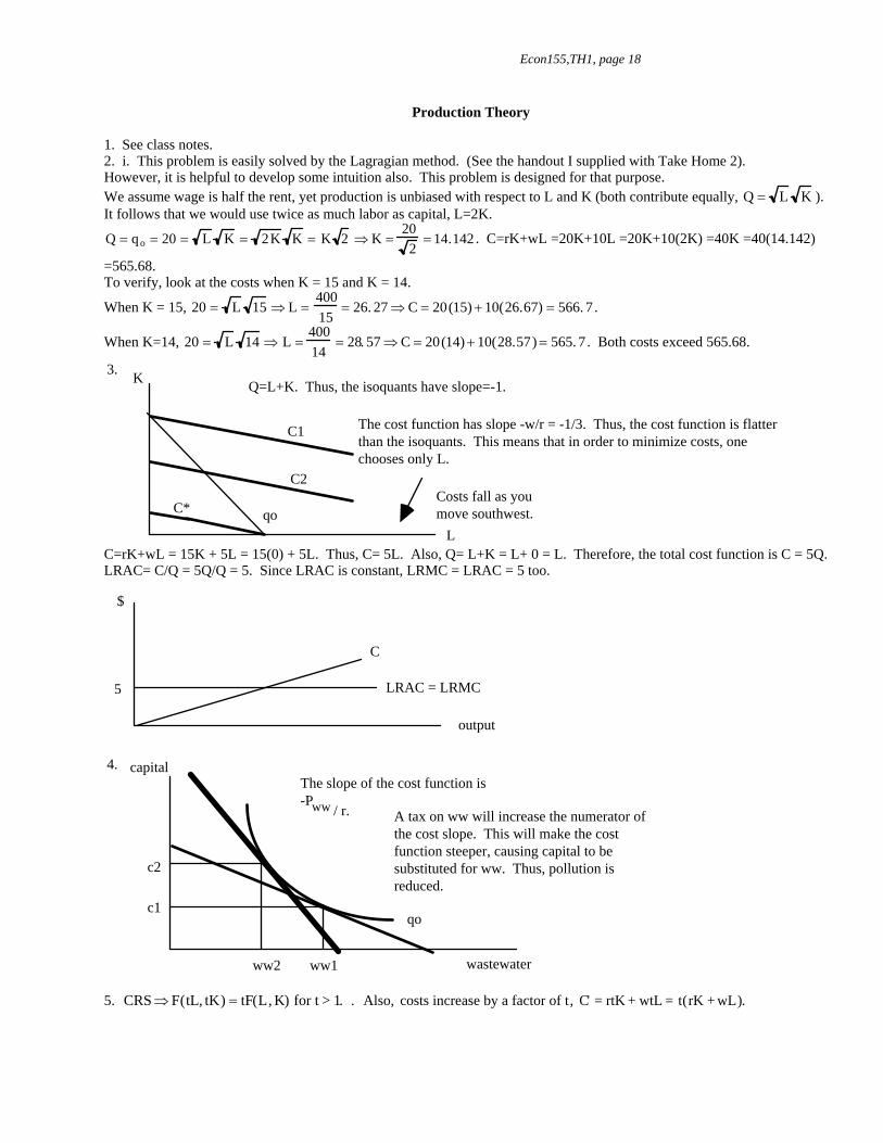
Econ155,TH1, page 18
Production Theory 1. See class notes. 2. i. This problem is easily solved by the Lagragian method. (See the handout I supplied with Take Home 2). However, it is helpful to develop some intuition also. This problem is designed for that purpose. We assume wage is half the rent, yet production is unbiased with respect to L and K (both contribute equally, Q = L K ). It follows that we would use twice as much labor as capital, L=2K.
Q = qo = 20 = L K = 2K K = K 2 ⇒ K =20
2= 14.142 . C=rK+wL =20K+10L =20K+10(2K) =40K =40(14.142)
=565.68. To verify, look at the costs when K = 15 and K = 14.
When K = 15, 20 = L 15 ⇒ L =40015
= 26. 27 ⇒ C = 20(15) + 10(26.67) = 566. 7.
When K=14, 20 = L 14 ⇒ L =40014
= 28. 57 ⇒ C = 20(14) + 10(28.57) = 565. 7. Both costs exceed 565.68.
L
K3.Q=L+K. Thus, the isoquants have slope=-1.
The cost function has slope -w/r = -1/3. Thus, the cost function is flatter than the isoquants. This means that in order to minimize costs, one chooses only L.
qoCosts fall as you move southwest.
C1
C2
C*
C=rK+wL = 15K + 5L = 15(0) + 5L. Thus, C= 5L. Also, Q= L+K = L+ 0 = L. Therefore, the total cost function is C = 5Q. LRAC= C/Q = 5Q/Q = 5. Since LRAC is constant, LRMC = LRAC = 5 too.
C
$
output
LRAC = LRMC5
wastewater
capital
qo
ww2 ww1
c1
c2
The slope of the cost function is -P ww / r. A tax on ww will increase the numerator of
the cost slope. This will make the cost function steeper, causing capital to be substituted for ww. Thus, pollution is reduced.
4.
5. CRS ⇒ F(tL, tK) = tF(L, K) for t > 1. . Also, costs increase by a factor of t, C' = rtK + wtL = t(rK + wL).

Econ155,TH1, page 19
At Q=5, C= 2(2) + 1(3) = 7. When C' = 70 = 10(7) and it follows that t = 10. Thus, when C' = 70, K = 10(2) = 20 and L = 10(3) = 30.

Econ155,TH1, page 20
6. From class we know that the cost minimizing solution is always at the vertex of the Leontief isoquant. The ray of vertices is .5L = K or L = 2K. It follows that C= rK+wL = 5K+5L = 5K+5(2K) = 15K. Also, Q=.5L=K. Therefore, LRTC = C = 15Q. Thus, LRAC = C/Q =15 = LRMC since average cost is constant.
C
$
output
LRAC = LRMC15
qo
skilled (union) workers
unskilled workers
7.The slope of the cost function is -w u /ws
.
As the minimum wage rises, the slope gets steeper. That is, as the cost differential falls, skilled labor is substituted for unskilled labor. Thus, unions support the minimum wage because it puts more of their own to work, not because they like to support their fellow workers!
us1us2
s1
s2
8. i. According to the graph, F(2L,2K)<2F(L,K) and so on. Thus, there are DRS.
LRMC
LRAC
ii. LRTCC, $
output
DRS imply an increasing LRTC curve. Thus, the slope, LRMC is rising. This pulls LRAC higher as well.

Econ155,TH1, page 21
L
Kqo
1.5qo2qo
L 2L 4L
K
2K
4K
iii.
LRAC
ii.C, $
output
SRAC
SECTION 3
Competition and Collusion 1. Samantha's Subs is a firm in a perfectly competitive industry. Assume that the industry price is $5.00. The cost structure for this firm follows. QUANTITY(units): 0 1 2 3 4 5 6 7 TOTAL COST($): 4 8 11 13 16 20 25 31 TFC: It is often MR: helpful to MC: calculate TVC: these AC: first. AVC: i. To maximize profits the firm should produce: ii. The firm's average variable costs are: iii. The firm's maximum profits are: iv. The firm would close in the short run if the market price dipped below: v. True or False: Given the current situation, firms will enter the industry. Explain. vi. True or False: If the industry price were $4.00 firms will leave the industry. Explain. vii. True or False: A monopoly maximizes profits by choosing Q where MR = MC and P where Q intersects demand. Explain. 2. Katie's Kitchen is a monopoly facing demand p=60-6q. The cost structure for this firm follows. QUANTITY(units): 0 1 2 3 4 5 6 TOTAL COST($): 2 8 16 26 38 58 80 i. What is the marginal revenue function for this firm? ii. In order to maximize profits how many units must the firm produce? iii. The firm will close immediately if price falls below $___: iv. True or False: Katie's Kitchen is currently earning positive economic profit so it stands to reason that it is in a long run situation. 3. A perfectly competitive industry is said to have increasing costs if whenever firms enter the industry in response to the presence of pure economic profit, the increased demand for factors of production causes factor costs, and thus
Econ155,TH1, page 22
the firms' average costs, to increase. Sketch the long run supply curve for the industry in the presence of increasing costs. Hint: the industry long run supply curve in your notes is horizontal because we implicitly assumed that costs remained constant throughout all adjustment processes. However, our application concerning land values explicitly assumes increasing costs! 4. Graphically illustrate and explain the following: i. A monopoly that can conceivably offer the same profit maximizing quantity at two different prices. (What does this imply about monoplolies?) ii. A monoploly that would close immediately. iii. Why might requiring monopolies to charge a competitve price be unrealistic. If one were forced to regulate monopoly prices, what price might be fair to both consumers and monpolists? Use a graph!

Econ155,TH1, page 23
5. i. Explain how the following "prisoner's dilemma" type game can explain competition and collusion among duopolists. All values represent potential profits. ii. What is the (Nash) equilibrium solution? WHY is this an equilibrium (draw the proper arrows and briefly explain)? A\B Firm B Cheat Collude Firm A Cheat 10\10 30\5 Collude 5\30 20\20 6. The market demand curve for an duopolistic industry is given by p = 36 - 3Q. Assume that marginal cost is 0 (constant) for each duopolist. Note: MC=0 is not a trick! It just makes the calculations a bit simpler! i. Find the Cournot equilibrium price, quantity and profits for each firm. State and graph the reaction functions of each firm. ii. Find the Stackelberg equilibrium price, quantity and profits for each firm. State and graph the reaction functions of each firm. iii. Find the Bertrand equilibrium price, quantity and profits for each firm. iv. Find the Cartel equilibrium price, quantity and profits for each firm. 7. In the spatial model of monopolistic competition, assume there are 1000 total customers and 5 firms, each with TC = 100 + 4Q. Calculate the price paid by the consumer if one way transportation costs equals $t. Is the optimal number of firms greater than, less than, or equal to 5? Explain.
Factor Markets
1. A monopsonist's demand for labor is given by w = 18 - L and its AFC curve is given by w = 3 + 2L. i. How many laborers will the monopsonist hire and what wage will he offer? ii. How many laborers will the monopsonist hire with a minimum wage of $11? 2. Are the following statements True, False or Uncertain? Explain your conclusions. When 'uncertain' provide conditions that would make the statement true or false. i. The marginal revenue product (MRP) curve is a firms demand curve for a factor of production. ii. An increase in the demand for bicycles will shift the MRP (Marginal Revenue Product) of bicycle factory workers left, causing the output (Q) of bicycle firms to rise. iii. A decline in the demand for movie tickets causes a decline in demand for cinema ushers. This is an example of derived demand. iv. The market output rule that is analogous to the market input rule of MRP = MRC is P = MC. v. After hiring 30 units of the variable input labor, a firm determines that MRC (of labor) = 20 dollars, and the MRP (of labor) = 23 dollars. Thus, the firm should decrease the use of labor. vi. An increase in the wage rate will cause the demand curve for labor to shift. 3. Explain how a price taking monopsonist differs from a typical perfectly competitive firm. In particular, will
wage equal marginal (labor) cost? Why or why not? 4. Explain the relationship between the rental rate and the interest rate. SECTION 3 SOLUTIONS 1. Samantha's Subs is a firm in a perfectly competitive industry. Assume that the industry price is $5.00. QUANTITY(units): 0 1 2 3 4 5 6 7 TOTAL COST($): 4 8 11 13 16 20 25 31 TFC=TC when Q=0: 4 4 4 4 4 4 4 4 MR=P in P.C. 5 5 5 5 5 5 5 5

Econ155,TH1, page 24
MC= TCQ
∆∆
: - 4 3 2 3 4 5 6
TVC=TC-TFC: 0 4 7 9 12 16 21 27
AC= TCQ
: - 8 5.5 4.33 4 4 4.17 4.43
AVC= TVCQ
: - 4 3.5 3 3 3.2 3.5 3.86
i. To maximize profits the firm should produce Q = 6, where MR = 5 = MC. ii. The firm's average variable costs are 3.5. iii. The firm's maximum profits are TR - TC = PxQ - TC = 5(6) - 25 = 5 > 0. iv. The firm would close in the short run if the market price dipped below minimum AVC = 3. v. True: Given the current situation, firms will enter the industry since profit >0 and there are no barriers to entry. vi. False: If the industry price were $4.00, MR = MC at Q = 5. Here, profit = TR - TC = PxQ-TC= 20-20 =0. vii. True. 2. Katie's Kitchen is a monopoly facing demand p=60-6q. QUANTITY(units): 0 1 2 3 4 5 6 TOTAL COST($): 2 8 16 26 38 58 80 Price=60-6Q: 60 54 48 42 36 30 24 TFC=TC when Q=0: 2 2 2 2 2 2 2 MR=60-12Q: 60 48 36 24 12 0 -12
MC= TCQ
∆∆
: - 6 8 10 12 20 22
TVC=TC-TFC: 0 6 14 24 36 56 78
AC= TCQ
: - 8 8 8.67 9.5 11.6 13.33
AVC= TVCQ
: - 6 7 8 9 11.2 13
i. The marginal revenue function for this firm is the derivative of TR=PxQ; MR = 60 - 12Q. ii. In order to maximize profits the firm must produce Q = 4 where MR = MC = 12. iii. The firm will close immediately if price falls below minimum AVC = 6. iv. True: Katie's Kitchen is currently earning positive economic profit so it stands to reason that it is in a long run situation because of the presence of barriers to entry (TR-TC= 36(4)-38=106).
Econ155,TH1, page 25
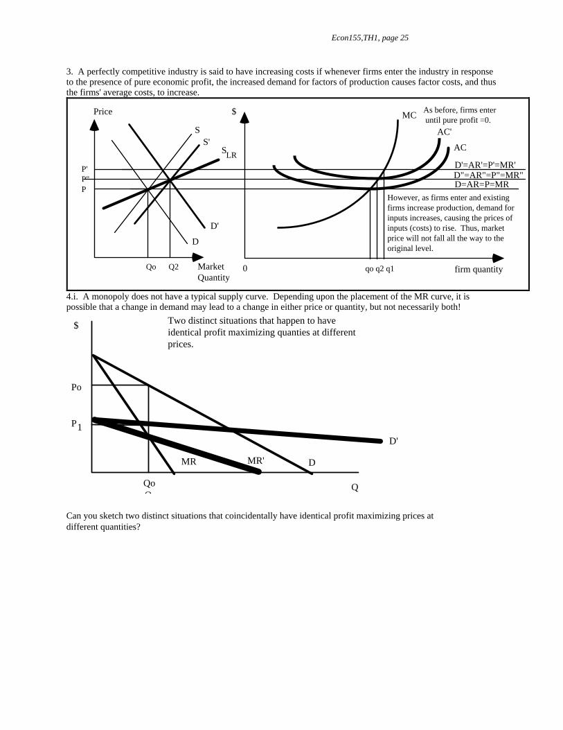
3. A perfectly competitive industry is said to have increasing costs if whenever firms enter the industry in response to the presence of pure economic profit, the increased demand for factors of production causes factor costs, and thus the firms' average costs, to increase.
S
D
D'
Price $
Market Quantity
firm quantity
MC
AC
0
D'=AR'=P'=MR'
D=AR=P=MR
S'
D"=AR"=P"=MR"
SLR
However, as firms enter and existing firms increase production, demand for inputs increases, causing the prices of inputs (costs) to rise. Thus, market price will not fall all the way to the original level.
qo q2 q1Qo Q2
P' P" P
AC'
As before, firms enter until pure profit =0.
4.i. A monopoly does not have a typical supply curve. Depending upon the placement of the MR curve, it is possible that a change in demand may lead to a change in either price or quantity, but not necessarily both!
$
DMR
Q
Po
Qo
MR'
D'
P1
Two distinct situations that happen to have identical profit maximizing quanties at different prices.
Q
Can you sketch two distinct situations that coincidentally have identical profit maximizing prices at different quantities?

Econ155,TH1, page 26
4.ii.
ACAVC
Price
Quantity
D
MR
MC
P?
Q?0
In this scenario, if the firm were to produce at a positive level of output while minimizing losses, P<AVC, so TR<TVC. Clearly, the firm is better off shutting down immediately since if it stays open it must pay all TFC and some labor costs (TVC) out of pocket. By closing it is only liable for TFC (TVC=0).
4.iii. Also see handout.
D
MR
Q
$
LRAC
LRMC
Pm Pf
Pc
This region denotes monopoly profits.
Pc and Qc represent a competive outcome for they are consistent with P=MC. That is, production continues until the cost of the last unit equals the price the firm receives for it. However, if the monopoly has economies of scale, this outcome will place the monopoly into a loss situation (D=P<LRAC, so .
Π<0)
Thus, Pf and Qf are referred to as a "fair" prices and quantity, balancing the the utility of the consumer with firm profits. Note, this compromise ensures that profits are normal, just as in the competitve outcome; but in contrast, price is higher than the cost of producing the next unit. Thus, this outcome is merely "close to" the competitive outcome.
Note: when allowed to choose for itself, a monopoly will always choose to produce on the elastic portion of its demand curve for the quantity chosen will always imply MR>0. See class notes.
Qm Qf Qc

Econ155,TH1, page 27
5.i. See handout. 5.ii. Even if the two duopolists agree to collude, each could increase profits by cheating (increasing output). Once one firm realizes that his former partner is cheating, he will no longer honor the agreement. The outcome (A, B)= (cheat, cheat) is the Nash equilibrium.
Cheat
Collude
ColludeCheatAB
10
10
20
20
5
30
30
5*
6. Duopoly: Consider an oligopolistic industry with two firms. 6.i. Cournot Quantity Competition (Symmetric Game): Assume industry demand is given by , where each firm has only labor costs, . Each firm has half the market, so market demand can be expressed as .
P 36 3Q= −
1 2MC MC 0= =
1 2P 36 3Q 3Q= − −
Since firm 1 controls half the market, it faces demand 1P 36 3Q 3Q= − − 2 where Q 2 is fixed. (Similarly firm 2 has demand 1 2P 36 3Q 3Q= − − .) Marginal Revenue for firm 1 is:
( ) ( ) ( )21 2 1 1 1 2 111
1 2 11 1 1 1
(36 3Q 3Q )Q 36Q 3Q 3Q QP QTRMR 36 3Q 6QQ Q Q Q
∂ − − ∂ − −∂ ⋅∂= = = = = − −
∂ ∂ ∂ ∂.
To maximize profits the firm will produce the quantity commensurate with MR=MC. 1 1 2 1 1MR MC 36 3Q 6Q 0 Q 6 0.5Q= ⇒ − − = ⇒ = − 2 . The equation, 1Q 6 0.5Q= − 2 , is called firm 1's reaction function. By
symmetry, firm 2's reaction function is 2 1Q 6 0.5Q= − .
Q1
Q2
Firm 1's Reaction Function
Firm 2's Reaction Function
The reaction functions are equal at (Q1, Q2) = (4,4). This is a stable equilibrium.
12
126
6
4
4
Industry price is . P 36 6(4 4) 12= − + =Thus, for each firm, Henceforth, note that . i i i iTR 12(4) 48 TR TC 48 0 48.= = ⇒ Π = − = − = i iMC 0 TR= ⇒ = Πi

Econ155,TH1, page 28
6.ii. Stackelberg Competition (Quantity Leader): Assume that firm 1 (leader) knows firm 2's (follower) reaction function. It can increase profits by incorporating this information. Again industry price is . The leader substitutes the reaction function for firm 2 into its demand, 1P 36 3Q 3Q= − − 2
( )1 1 13P 36 3Q 3 6 0.5Q 18 Q2
= − − − = − . 2
1 1 1 1 13TR 18Q Q MR 18 3Q2
= − ⇒ = − . The profit maximizing quantity is found by setting 1 1 1 1MR MC 18 3Q 0 Q 6= ⇒ − = ⇒ = . The follower's quantity is then determined by its reaction, 2Q 6 0.5(6) 3= − = . Industry output is Q=9.
Q1
Q2Firm 1's (Leader) Reaction Function
Firm 2's (Follower) Reaction Function
The reaction functions are equal at (Q1, Q2) = (6,3). This is a stable equilibrium.
12
6
6
3
Industry price is . P 36 3(9) 9= − = ( ) ( )i i 2 2TR 9 6 54, TR 9 3 27Π = = = Π = = = . Note that the leader's profit is larger than in the Cournot scenario, whereas the follower's profit is less. Thus, having information that your competitors do not have is a blessing for you and a curse for them! 6.iii. Bertrand (Price) Competition: Here the duopolists act as perfect competitors until P=MC.
iP MC 0 36 3Q 0 Q 12 Q 6= = ⇒ − = ⇒ = ⇒ = for each firm. i iTR 0Π = = for each firm. 6.iv. Cartel (Monopoly outcome):
set2
1 2TR 36Q 3Q MR 36 6Q MC 0 Q 6 Q Q 3 P 36 3(6) 18= − ⇒ = − = = ⇒ = ⇒ = = ⇒ = − = . ( )i iTR 18 3 54Π = = = for each firm. Note that profits for both firms are higher than all other scenarios.
7. 100TC=100+4Q AC= 4Q
⇒ + . The consumers' price is P AC 2dt= + where 1d4N
= is the average one-way
distance a consumer must travel and t is the one-way fare. The number of customers per firm is 1000QN
= .
The goal is to minimize with respect to N: P AC 2dt= +
( )
100 14 2 t100 1 1000 14N4 2 t 0.1N 4 t
AC 2dt Q 4N N 2NPN N N N N
⎛ ⎞⎜ ⎟⎛ ⎞⎜ ⎟∂ + + ⎜ ⎟⎛ ⎞ ⎛⎜ ⎟⎛ ⎞ ⎛ ⎞ ⎛ ⎞⎝ ⎠∂ + + ∂ + +⎜ ⎟ ⎜⎜ ⎟ ⎜ ⎟ ⎜ ⎟⎜ ⎟∂ +∂ ⎝ ⎠ ⎝ ⎠ ⎝ ⎠⎝ ⎠ ⎝ ⎠ ⎝= = = =
∂ ∂ ∂ ∂ ∂
⎞⎟⎠
set
2P t0.1 N 0 N 5tN 2
−∂ ⎛ ⎞= − = ⇒ =⎜ ⎟∂ ⎝ ⎠ is the optimal number of firms.
Thus, if , the optimal number of firms is t 5.92≤ 5≤ . If t >5.92, the optimal number of firms is >5.

Econ155,TH1, page 29

Intermediate Macro Theory Review
1
Intermediate Macroeconomics Review Sample Problem Set with Solutions
1. i) Illustrate and explain how a decrease in the expected price levels shifts aggregate supply to the right.
ii) . In an article entitled "Strong Chairmen Weaken the Fed" in the Wall Street Journal (week of April 22, 1991), Jerry Jordan states: "The secrecy about what actually goes on in an Open Market Committee meeting is self-imposed. And the Fed watcher industry thrives on secrecy. Other central banks, such as the German Bundesbank, hold a press conference and announce their policy decisions at the end of their meetings, leaving no room for doubt or speculation about their actions. The Fed contributes to short-term volatility in markets by making the rest of us guess at what they are really up to." What model of the macroeconomy do you think the author is using? Show and explain why secrecy regarding policy actions leads to output instability. 2) i) New Classical macroeconomists argue that an announced, credible policy of expanding the money supply could decrease aggregate output rather than increase it. Using the New Classical model, use the labor market and AS\AD (Ys\Yd) to illustrate and explain the reasoning behind this argument. ii) Would (a) a Keynesian economist, and (b) a monetarist economist agree with the assumptions and conclusions in (i)? In each case, use the labor market and AS\AD (Ys\Yd) to thoroughly explain the differences. 3) i) Show and explain how "labor fooling" in the labor market can lead to variations in the slope of the aggregate supply curve under (a) new classical, (b) keynesian and (c) monetarist assumptions. ii) Use the Phillips Curve analysis to illustrate and explain how "labor fooling" can lead to variations in output and inflation under (a) new classical, (b) keynesian and (c) monetarist assumptions. 4) Assume the following information: C = 300 + .8Ydis; I = 200; G = 300; T = 50; EX = 100; IM = 20+0.1Ydis. i) What are the equilibrium values of GDP and savings? ii) Graph the Keynesian Cross. Label it with YE and the current value of autonomous expenditures.
5) Show how an increase in the money supply affects aggregate demand via IS/LM when:
i) investment demand is interest inelastic.
ii) investment demand is interest elastic. 6) Show how an increase in government spending affects the aggregate demand curve: i. when you have a steep LM curve ii. when you have a flat LM curve. iii. Which school of thought would you attribute to (i)? To (ii)? Explain. 7) Assume the country currently faces a Balance of Payments (external) surplus, with an internal balance, fixed exchange rates, and a high degree of international capital mobility. i. Of the two, do you recommend fiscal or monetary policy to achieve a simultaneous internal and external balance? Illustrate, and explain the net benefits of each policy. ii. Now assume we are under floating exchange rate system. Illustrate and explain how else a simultaneous internal and external balance might be achieved.
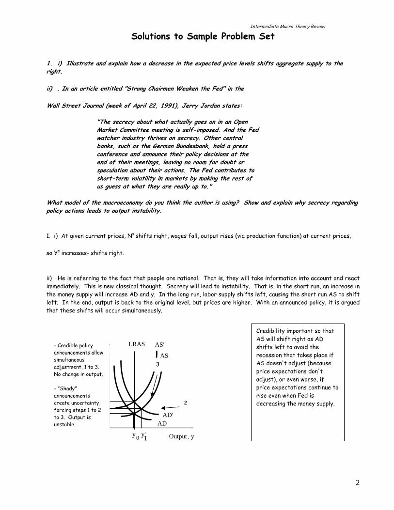
Intermediate Macro Theory Review
2
.
Solutions to Sample Problem Set
1. i) Illustrate and explain how a decrease in the expected price levels shifts aggregate supply to the right.
ii) . In an article entitled "Strong Chairmen Weaken the Fed" in the
Wall Street Journal (week of April 22, 1991), Jerry Jordan states: "The secrecy about what actually goes on in an Open Market Committee meeting is self-imposed. And the Fed watcher industry thrives on secrecy Other central banks, such as the German Bundesbank, hold a press conference and announce their policy decisions at the end of their meetings, leaving no room for doubt or speculation about their actions. The Fed contributes to short-term volatility in markets by making the rest of us guess at what they are really up to." What model of the macroeconomy do you think the author is using? Show and explain why secrecy regarding policy actions leads to output instability.
1. i) At given current prices, Ns shifts right, wages fall, output rises (via production function) at current prices,
so Ys increases- shifts right.
ii) He is referring to the fact that people are rational. That is, they will take information into account and react immediately. This is new classical thought. Secrecy will lead to instability. That is, in the short run, an increase in the money supply will increase AD and y. In the long run, labor supply shifts left, causing the short run AS to shift left. In the end, output is back to the original level, but prices are higher. With an announced policy, it is argued that these shifts will occur simultaneously.
Credibility important so that AS will shift right as AD shifts left to avoid the recession that takes place if AS doesn't adjust (because price expectations don't adjust), or even worse, if price expectations continue to rise even when Fed is decreasing the money supply.
AS'
ADAD'
0
Prices
Output , y
AS
p1
po
y
LRAS
y'1
- Credible policy announcements allow simultaneous adjustment, 1 to 3. No change in output. - "Shady" announcements create uncertainty, forcing steps 1 to 2 to 3. Output is unstable.
3
2
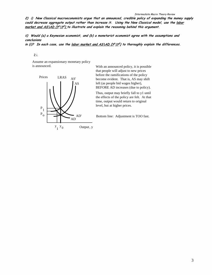
Intermediate Macro Theory Review
3
2) i) New Classical macroeconomists argue that an announced, credible policy of expanding the money supply could decrease aggregate output rather than increase it. Using the New Classical model, use the labor market and AS\AD (Ys\Yd) to illustrate and explain the reasoning behind this argument. ii) Would (a) a Keynesian economist, and (b) a monetarist economist agree with the assumptions and conclusions in (i)? In each case, use the labor market and AS\AD (Ys\Yd) to thoroughly explain the differences.
ADAD'
AS'
0
With an announced policy, it is possible that people will adjust to new prices before the ramifications of the policy become evident. That is, AS may shift left (as people bid wages higher), BEFORE AD increases (due to policy).
y1
Thus, output may briefly fall to y1 until the effects of the policy are felt. At that time, output would return to original level, but at higher prices.
Assume an expansionary monetary policy is announced.
Bottom line: Adjustment is TOO fast.
2.2.i.
Prices
Output , y
AS
p1
po
y
LRAS

Intermediate Macro Theory Review
4
2. ii. Ns(NewClass:P=3Po) New Classical nominal wage, w Ns(Mon:P=2Po) 3w0 Ns(Keynes:P=Po) 2.5w0 Monetarists 2w0
Keynesian w0 Nd(P=3Po) Nd(P=Po)
NNCL NM NK Labor, N
Prices Ys
ncl Ys
M
YK F(K,L) YM
Ys
K
Yd
1
Yd
NNCL Nm NK Labor, N YNCL YM YK Y
3P0
2P0
P0
Keynesianism does not assume any adjustment to expectations. Monetarism assumes at most partial adjustment in short run because of adaptive expectations. Rational expectations imply that if a policy is systematically carried out, people will adjust expectations concerning the impact on prices immediately and perfectly.
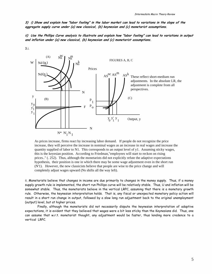
Intermediate Macro Theory Review
5
3) i) Show and explain how "labor fooling" in the labor market can lead to variations in the slope of the aggregate supply curve under (a) new classical, (b) keynesian and (c) monetarist assumptions. ii) Use the Phillips Curve analysis to illustrate and explain how "labor fooling" can lead to variations in output and inflation under (a) new classical, (b) keynesian and (c) monetarist assumptions. 3.i.
(A)
(B) (C)
N
N
y
F
Prices
Output, y
W
AS
N* N' N1 1
Nd(p )o
Nd (p )1
y y' y
011
0 1 1y y' y
p1
po
AS
As prices increase, firms react by increasing labor demand. If people do not recognize the price increase, they will perceive the increase in nominal wages as an increase in real wages and increase the quantity supplied of labor to N1. This corresponds to an output level of y1. Assuming sticky wages, this is the keyesian position. According to Friedman,"employees will start to reckon on rising prices.." (. 252). Thus, although the monetarists did not explicitly refute the adaptive expectations hypothesis, their position is one in which there may be some wage adjustment even in the short run (N'1). However, the new classicists believe that people are wise to the price change and will completely adjust wages upward (Ns shifts all the way left).
NsNs
Nsk
k
m
m
nc
ncAS
FIGURES A, B, C
These reflect short-medium run adjustments. In the absolute LR, the adjustment is complete from all perspectives.
ii. Monetarists believe that changes in income are due primarily to changes in the money supply. Thus, if a money supply growth rule is implemented, the short run Phillips curve will be relatively stable. Thus, U and inflation will be somewhat stable. Thus, the monetarists believe in the vertical LRPC, assuming that there is a monetary growth rule. Otherwise, the keynesian interpretation holds. That is, any fiscal or unexpected monetary policy action will result in a short run change in output, followed by a slow long run adjustment back to the original unemployment (output) level, but at higher prices. Finally, although the monetarists did not necessarily dispute the keynesian interpretation of adaptive expectations, it is evident that they believed that wages were a bit less sticky than the Keynesians did. Thus, one can assume that w.r.t. monetarist thought, any adjustment would be faster, thus lending more credence to a vertical LRPC.

Intermediate Macro Theory Review
6
LRPC
PC
PC'
U
ρ
4) Assume the following information: C = 300 + .8Ydis; I = 200; G = 300; T = 50; EX = 100; IM = 20+0.1Ydis. i) What are the equilibrium values of GDP and savings? ii) Graph the Keynesian Cross. Label it with YE and the current value of autonomous expenditures. 4) Assume the following information: C = 300 + .8Ydis; I = 200; G = 300; T = 50; EX = 100; IM = 20+0.1Ydis. i.
300 .8( 50) 200 300 (100 (20 0.1( 50)))
0.7 845( . exp .) 2816.67
Y Y Y
Y Y aut YE
= + − + + + − + −
− = ⇒ =
ii) Draw Keynesian Cross noting that autonomous expenditures = 845
a+I+G+EX-0.7T
autonomous expenditures
= 845
AE C+I+G+NX
Y
45 o
2816.67
5) Show how an increase in the money supply affects aggregate demand via IS/LM when:
i) investment demand is interest inelastic.
ii) investment demand is interest elastic.
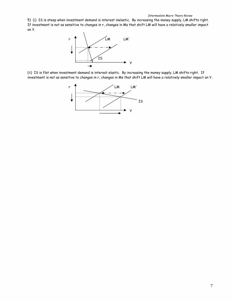
Intermediate Macro Theory Review
7
5) (i) IS is steep when investment demand is interest inelastic. By increasing the money supply, LM shifts right. If investment is not as sensitive to changes in r, changes in Ms that shift LM will have a relatively smaller impact on Y. r LM LM' IS Y (ii) IS is flat when investment demand is interest elastic. By increasing the money supply, LM shifts right. If investment is not as sensitive to changes in r, changes in Ms that shift LM will have a relatively smaller impact on Y. r LM LM' IS Y
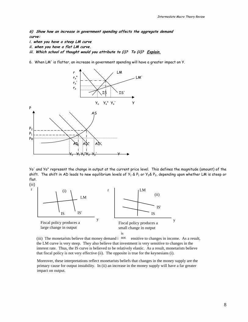
Intermediate Macro Theory Review
6) Show how an increase in government spending affects the aggregate demand curve: i. when you have a steep LM curve ii. when you have a flat LM curve. iii. Which school of thought would you attribute to (i)? To (ii)? Explain. 6. When LM' is flatter, an increase in government spending will have a greater impact on Y. r LM ro" LM' ro' ro IS IS' Yo Yo" Yo' Y P AS P2
P1
Po AD AD" AD' Yo Y1 Yo"Y2 Yo' Y Yo' and Yo" represent the change in output at the current price level. This defines the magnitude (amount) of the shift. The shift in AD leads to new equilibrium levels of Y1 & P1 or Y2& P2, depending upon whether LM is steep or flat. (iii)
r LM
ISIS'
yFiscal policy produces a large change in output
Fiscal policy produces a small change in output
(i)(ii)
(iii) The monetarists believe that money demand i y sensitive to changes in income. As a result, the LM curve is very steep. They also believe that stment is very sensitive to changes in the interest rate. Thus, the IS curve is believed to be rethat fiscal policy is not very effective (ii). The opp
r
LM
IS IS'y
Moreover, these interpretations reflect monetaristsprimary cause for output instability. In (ii) an incrimpact on output.
s ver inve
is not
8
latively elastic. As a result, monetarists believe osite is true for the keynesians (i).
beliefs that changes in the money supply are the ease in the money supply will have a far greater
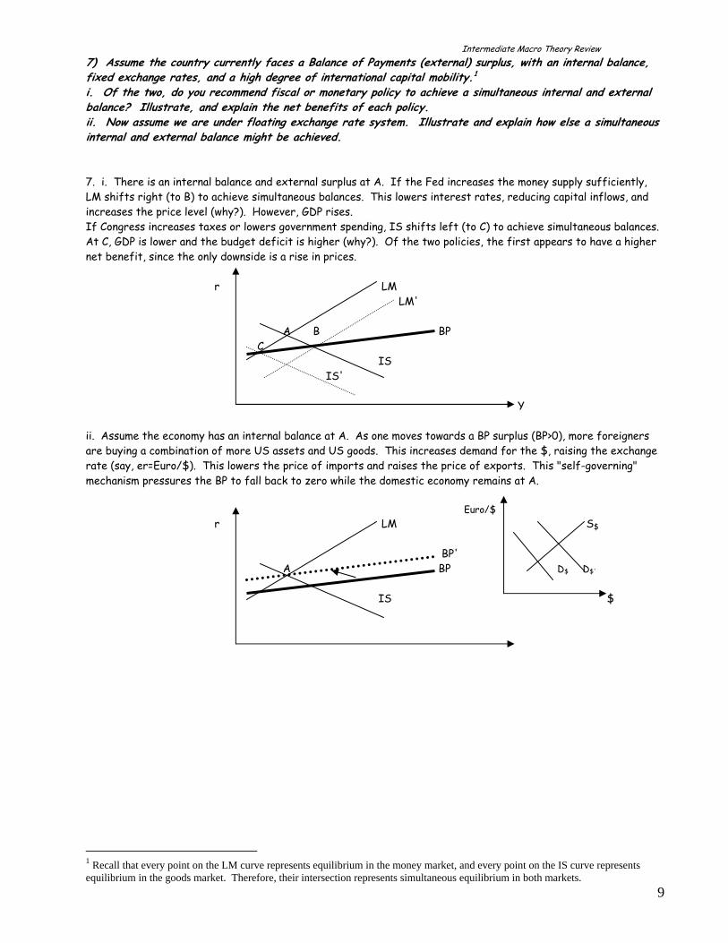
Intermediate Macro Theory Review
9
7) Assume the country currently faces a Balance of Payments (external) surplus, with an internal balance, fixed exchange rates, and a high degree of international capital mobility.1i. Of the two, do you recommend fiscal or monetary policy to achieve a simultaneous internal and external balance? Illustrate, and explain the net benefits of each policy. ii. Now assume we are under floating exchange rate system. Illustrate and explain how else a simultaneous internal and external balance might be achieved. 7. i. There is an internal balance and external surplus at A. If the Fed increases the money supply sufficiently, LM shifts right (to B) to achieve simultaneous balances. This lowers interest rates, reducing capital inflows, and increases the price level (why?). However, GDP rises. If Congress increases taxes or lowers government spending, IS shifts left (to C) to achieve simultaneous balances. At C, GDP is lower and the budget deficit is higher (why?). Of the two policies, the first appears to have a higher net benefit, since the only downside is a rise in prices.
r LM LM' A B BP C IS IS' Y ii. Assume the economy has an internal balance at A. As one moves towards a BP surplus (BP>0), more foreigners are buying a combination of more US assets and US goods. This increases demand for the $, raising the exchange rate (say, er=Euro/$). This lowers the price of imports and raises the price of exports. This "self-governing" mechanism pressures the BP to fall back to zero while the domestic economy remains at A. Euro/$ r LM S$
BP'
A BP D$ D$'
IS $
1 Recall that every point on the LM curve represents equilibrium in the money market, and every point on the IS curve represents equilibrium in the goods market. Therefore, their intersection represents simultaneous equilibrium in both markets.
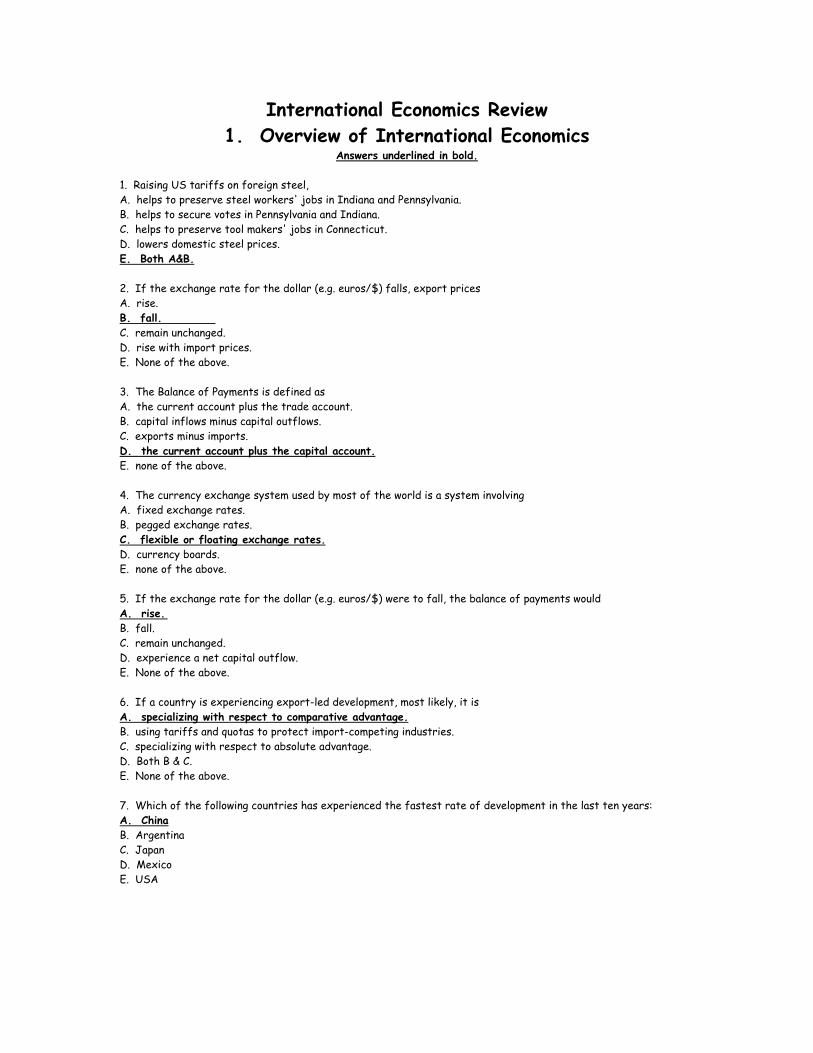
International Economics Review 1. Overview of International Economics
Answers underlined in bold. 1. Raising US tariffs on foreign steel, A. helps to preserve steel workers' jobs in Indiana and Pennsylvania. B. helps to secure votes in Pennsylvania and Indiana. C. helps to preserve tool makers' jobs in Connecticut. D. lowers domestic steel prices. E. Both A&B. 2. If the exchange rate for the dollar (e.g. euros/$) falls, export prices A. rise. B. fall. C. remain unchanged. D. rise with import prices. E. None of the above. 3. The Balance of Payments is defined as A. the current account plus the trade account. B. capital inflows minus capital outflows. C. exports minus imports. D. the current account plus the capital account. E. none of the above. 4. The currency exchange system used by most of the world is a system involving A. fixed exchange rates. B. pegged exchange rates. C. flexible or floating exchange rates. D. currency boards. E. none of the above. 5. If the exchange rate for the dollar (e.g. euros/$) were to fall, the balance of payments would A. rise. B. fall. C. remain unchanged. D. experience a net capital outflow. E. None of the above. 6. If a country is experiencing export-led development, most likely, it is A. specializing with respect to comparative advantage. B. using tariffs and quotas to protect import-competing industries. C. specializing with respect to absolute advantage. D. Both B & C. E. None of the above. 7. Which of the following countries has experienced the fastest rate of development in the last ten years: A. China B. Argentina C. Japan D. Mexico E. USA
International Economics Review
8. Do lower wages in developing countries almost always lure companies away from developed countries? A. No, because transportation costs and poorly developed infrastructure such as roads and ports may make total costs even higher than in a developed nation where workers earn a higher wage. B. Yes, because labor is always the highest cost associated with production. C. No, total costs depend on productivity, so one must compare wages/marginal product. D. Both A&C. E. None of the above. 9. The World Trade Organization (WTO) and regional trade pacts such as NAFTA, ASEAN, and the EU promote trade by A. raising trade barriers. B. raising quotas. C. lowering tariffs and quotas. D. imposing monetary unification (single currency) E. None of the above. 10. Even though barriers to trade reduce overall utility, why do countries maintain some barriers to trade? A. To protect jobs. B. To protect historically or culturally important industries. C. To protect fledgling industries. D. Both A&C. E. All the above. 11. When countries engage in trade, A. they tend to specialize. B. they exploit comparative advantages. C. they increase consumption and utility. D. they lose some jobs because of structural adjustment. E. All the above. 12. During the Asian Banking Crisis of 1997-98, capital inflows diminished because of falling investor confidence in the "zaibatsu" type relationship between corporations, banks and government. This initially led to a balance of payments deficit which gradually improved via A. first, currency depreciation, but eventually an increase in demand for Asian imports. B. first, currency depreciation, but eventually an increase in demand for Asian exports. C. first, currency appreciation, but eventually an increase in demand for Asian imports. D. first, currency appreciation, but eventually an increase in demand for Asian exports. E. none of the above. 13. If the Fed raises interest rates, the US would experience a net A. capital outflow. B. increase in exports. C. capital inflow. D. Both B&C. E. None of the above. 14. The World Bank and the International Monetary Fund deserve criticism because A. they have been attempting to tell other countries how to handle internal affairs. B. they have been charging interest on loans. C. they have been enforcing the same loan conditions, regardless of borrowers’ needs. D. they do not consider poverty or environmental issues in their mission statements. E. None of the above.
2

International Economics Review
15. India’s policy of supporting domestic import-competing industries has A. helped it to develop faster than the Pacific Rim. B. helped it to receive maximum gains from trade. C. helped to protect fledgling, capital-intensive, industries. D. caused it to develop slower than the Pacific Rim. E. Both C&D. 16. Which country (ies) has followed the fundamental tenets of the Heckscher-Ohlin Theorem? A. Pacific Rim countries like South Korea. B. India C. United States D. Both A&C. E. None of the above. 17. A "small" country: A. is one in which changes in production have no effect on world prices. B. usually specializes completely in the production of a single good. C. becomes comparatively more specialized when there is biased growth in its export sector. D. Both B&C. E. Both A&C. (Rybczinski Theorem) 18. Assume N1 is a large country that is beginning to experience growth. As a result, if N1 exports good x, post-trade world prices, ( )P Px y T
,
A. will return to the same level as in autarky. B. will stay constant. C. will fall. (terms of Trade effect) D. will rise. E. None of the above. 19. Tariffs are inefficient because A. they reduce consumption. B. they reduce utility. C. they eliminate portions of consumer surplus, i.e. produce dead weight loss. D. they preserve inefficient jobs. E. All the above. 20. The Bretton Woods agreement A. fixed the US dollar to a specific price per ounce of gold. B. fixed foreign currencies to the dollar. C. is a gold standard. D. is a market based currency system. E. Both A&B. 21. For a consumer who consumes two different goods, utility maximization occurs when the budget is exhausted, and the: A. ratio of marginal utility to price is the same for both goods. B. the budget constraint is just tangent to the indifference curve yielding greatest feasible utility. C. marginal utility of all goods is the same. D. Both A&B. E. None of the above.
3

International Economics Review
22. The |slope| of the production possibilities frontier at any point is:
A. MUxMU y
B. MCxMCy
C. PxPy
D. MU yMUx
E. Both B&C.
23. By undertaking a policy of propping its currency in 1994, Mexico was committed to A. selling its pesos in world currency markets. B. buying its pesos in world currency markets. C. reducing the value of Mexican assets held by foreigners. D. buying US dollars in world currency markets. E. Both C&D. 24. The currency board enforced by Argentina in the 1990s A. helped to reduce inflation. B. was a price control on exchange rate, $/Apeso. C. reduced monetary policy independence. D. was abandoned in 2001. E. All the above. 25. It is feared that regional trade pacts can sometimes reduce global trade because A. trade blocks are unstable. B. trade blocks promote trading within the block and not with the rest of the world. C. trade blocks require monetary union. D. Both A&C. E. None of the above. 26. The EMU (European Monetary Union) A. required potential members to attain stringent inflation and debt requirements. B. uses the “euro” currency. C. has as its members all the countries in the European Union. D. Both A&B. E. None of the above. 27. To successfully develop, Africa must A. discourage western dependence including foreign direct investment. B. promote human rights very slowly and carefully. C. encourage its educated workers to find jobs in the West. D. develop intercontinental infrastructure such as roads, ports, communications centers and railways. E. None of the above. 28. Are manufacturing wages in the US “set in China?” (Stolper-Samuelson and Factor Price Equalization Theorems) A. No, because the factor price equalization theorem suggests that only relative input prices are converging. B. No, because what matters most is the wage rate relative to productivity. C. No, because one must also consider transportation costs. D. Yes, absolutely, because low wages in China are forcing world prices lower. E. A, B, and C are all correct.
4

International Economics Review
29. Japan’s economic growth after World War II was helped by A. low interest rates due to its high savings rate. B. a reluctance by the West to force Japan to trade more freely because of its strategic importance. C. a well-educated population earning modest wages. D. Strong U.S. consumer demand. E. All the above. 30. Japan is not under as much pressure to reform its zaibatsu because A. it has a high domestic savings rate. B. it is more dependent on foreign direct investment than other Pacific Rim countries. C. it is less dependent on foreign direct investment than other Pacific Rim countries. D. Both A&C. E. Both A&B. 31. The events of 9-11-01 had a global economic impact A. from which we cannot fully recover. B. because it severely interrupted capital flows. C. because it crippled airline and related industries. D. because it raised interest rates world wide. E. None of the above. 32. Export “dumping” means A. a country is de-emphasizing its export sector. B. a foreign firm is selling its exports below domestic prices. C. a foreign firm is selling its exports below its production costs. D. a foreign firm is selling its exports below domestic import-competing production costs. E. a domestic import-competing firm has obtained greater market share. 33. Steak Fish Given these PPFs from the United States US 200 or 600 and the United Kingdom, UK 200 or 100 assume constant opportunity costs. Which country has a comparative advantage in steak? A. US B. UK C. Neither does. D. Both do. 34. Steak Fish Given these PPFs from the United States US 200 or 600 and the United Kingdom, UK 200 or 100 assume constant opportunity costs. Which is the most mutually beneficial terms of trade? (S:F)= A. (1:4) B. (1:1) C. (3:1) D. (2:1)
5
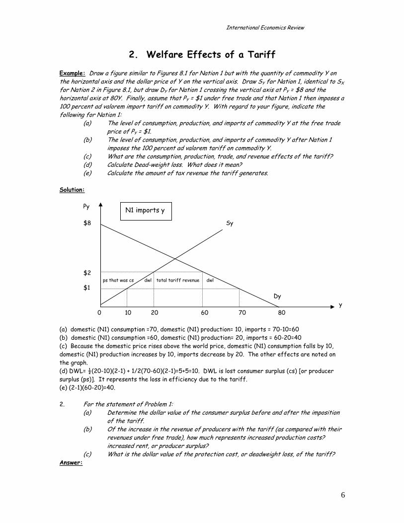
International Economics Review
2. Welfare Effects of a Tariff Example: Draw a figure similar to Figures 8.1 for Nation 1 but with the quantity of commodity Y on the horizontal axis and the dollar price of Y on the vertical axis. Draw SY for Nation 1, identical to SX for Nation 2 in Figure 8.1, but draw DY for Nation 1 crossing the vertical axis at PY = $8 and the horizontal axis at 80Y. Finally, assume that PY = $1 under free trade and that Nation 1 then imposes a 100 percent ad valorem import tariff on commodity Y. With regard to your figure, indicate the following for Nation 1:
(a) The level of consumption, production, and imports of commodity Y at the free trade price of PY = $1.
(b) The level of consumption, production, and imports of commodity Y after Nation 1 imposes the 100 percent ad valorem tariff on commodity Y.
(c) What are the consumption, production, trade, and revenue effects of the tariff? (d) Calculate Dead-weight loss. What does it mean?
(e) Calculate the amount of tax revenue the tariff generates. Solution: Py $8 Sy $2 ps that was cs dwl total tariff revenue dwl $1 Dy y
N1 imports y N1 imports y
0 10 20 60 70 80 (a) domestic (N1) consumption =70, domestic (N1) production= 10, imports = 70-10=60 (b) domestic (N1) consumption =60, domestic (N1) production= 20, imports = 60-20=40 (c) Because the domestic price rises above the world price, domestic (N1) consumption falls by 10, domestic (N1) production increases by 10, imports decrease by 20. The other effects are noted on the graph. (d) DWL= ½(20-10)(2-1) + 1/2(70-60)(2-1)=5+5=10. DWL is lost consumer surplus (cs) [or producer surplus (ps)]. It represents the loss in efficiency due to the tariff. (e) (2-1)(60-20)=40. 2. For the statement of Problem 1:
(a) Determine the dollar value of the consumer surplus before and after the imposition of the tariff.
(b) Of the increase in the revenue of producers with the tariff (as compared with their revenues under free trade), how much represents increased production costs? increased rent, or producer surplus?
(c) What is the dollar value of the protection cost, or deadweight loss, of the tariff? Answer:
6
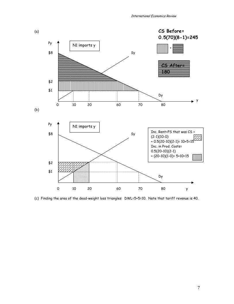
International Economics Review
(a) CS Before= 0.5(70)(8-1)=245 Py + $8 Sy $2 $1 Dy y
CS After= 180
N1 imports y
0 10 20 60 70 80 (b) Py $8 Sy $2 $1
N1 imports y
0 10 20 60 70
(c) Finding the area of the dead-weight loss triangles: DWL=5+5=10. N
Inc. Rent=PS that was CS = (2-1)(10-0) + 0.5(20-10)(2-1)= 10+5=15 Inc. in Prod. Costs= 0.5(20-10)(2-1) + (20-10)(1-0)= 5+10=15
Dy
80 y
ote that tariff revenue is 4
0.7

International Economics Review
3. How the Exchange Rate Affects Trade Patterns
$
L /$
D
S
When the price of a $ = er = L/$ increases we say that the $ has appreciated and the pound has depreciated. When L/$ decreases we say that the $ has depreciated and the $ has appreciated. Changes in Supply of $ occurs when there are: 1. Changes in domestic money supply 2. Changes in foreign central bank's holdings of $ 3. Capital Outflows stemming from
Change in the domestic interest rate. Change in foreign interest rate. Change in political climate. Change in economic or political expectations
4. Speculation that the dollar will depreciate Changes in Demand for $ occurs when there are: 1. Changes in demand for exports 2. Capital Inflows stemming from
Change in the domestic interest rate. Change in foreign interest rate. Change in political climate. Change in economic or political expectations
3. Speculation that the dollar will appreciate Example 1: Assume that the Fed decides to raise the discount rate. What effect does this have on the exchange rate? Other US rates will begin to rise as well. This makes investment in the US more appealing. Thus there will be an increase in the flow of capital ($ for investment) into the US. However, the foreign monies will have to be converted to US $ first. Thus, the demand for $ increases, causing an appreciation of the dollar. Note that we can express any change affecting $ and pounds in terms of either the market for $ or the market for pounds. For example, if U.S. interest rates rise, there could be a capital inflow
8

International Economics Review
for the U.S. and a capital outflow for Great Britain, as British investors seek higher paying assets in the U.S.. In both cases the $ appreciates since L/$ rises (or $/L falls, depending upon your perspective).
$/L
Example 2: How can the British government "prop" the pound? Hint: now look at the D&S for the pound in terms of the $. By buying L with $ the British can increase the demand for their own currency. This will increase the demand for the pound, increasing the price of a pound ($/L).
Equivalently, the purchase of L with dollars will increase the supply of dollars in the secondary market, thus decreasing L/$, the price of the dollar. That is, the dollar depreciates. Exercise: What should renewed hostilities by the IRA do to the value of the pound? Exchange Rate and Terms of Trade: Assume the following constant opportunity cost PPFs:
Paper Aluminum Products Foil
US 30 or 10 UK 20 or 20 This is consistent with the following competitive (P=MC) domestic price ratios for paper products and Aluminum Foil in the United States and the United Kingdom.
Paper Aluminum Products Foil
US $1 $3 UK L1 L1 Comparative Advantages in Currency terms: US: ($PP:$AF)= ($1:$3)
L$0 0
S$ L/$
S$’ S$”
D$’ D$’ D$”
9

International Economics Review
UK: (LPP:LAF)= (L1:L1) -AF costs the same as PP in the UK, whereas it is three times more expensive in the U.S..
Thus, the US has a comparative advantage in the production of Paper Products, whereas the comparative advantage of the UK is in Aluminum Foil. The only difference between this and earlier examples is that "opportunity cost" is now price. It is assumed that the market price reflects the true cost of producing the good. That is, if markets are competitive, relative prices do indeed yield comparative advantages. The exchange rate affects trade in the following way:
• If er = L/$ = 1/2, then the UK will import Paper Products from the US since they only cost $1 = L0.5 < L1, and the US will import Aluminum Foil from the UK since it only costs 1L = $2 < $3.
• If er = L/$ = 1/4, then the UK will import Paper Products and Aluminum Foil from the US since they only cost $1 = L0.25 < L1 and $3 = L0.75 < L1, respectively.
• If er = L/$ = 2/1, then the US will import Paper Products and Aluminum Foil from the UK since they only cost L1 = $0.5 < $1 and L1 = $0.5 < $1, respectively.
IMPORTANT! In order to have trade in both directions the exchange rate must fall within
the following range: 1 13 1
er< < . Note that 1/2 L/$ falls within this range.
Exercise: In example 1 of HW 1, for the US, the price of wine will be half the price of vodka. In Russia wine will cost five times that of vodka. Why? If the price of wine in the US is $10 a unit and the price of vodka in Russia is 10R per unit, what exchange rate range will guarantee trade in both directions?
4. The Balance of Payments Consists of:
1. Current Account: Trade in real goods and services 2. Capital Account: Capital flows
∴BP =CA+KA Official Reserve Account or Transactions: a. Domestic Currency, or more generally, b. M2 or M3.
The method of double entry bookkeeping implies that:
10
International Economics Review
CA+KA+ORT= 0 . ORT consist of central bank transactions in international reserve assets like gold, foreign exchange reserves, IMF credits, Special Drawing Rights (SDR - an IMF asset in terms of $, Y, DM, L, FF). ORT "back up" the domestic currency. If the foreign country wishes to exchange the currency for something "harder" this is the best they can do.
EXTERNAL BALANCE or BALANCE OF PAYMENTS EQUILIBRIUM.
means that together, the current and capital accounts balance to zero.
∴ORT= 0 .
EXTERNAL DEFICIT means that together,
the current and capital accounts are negative.
∴ORT>0 .
• We can view an ORT surplus as a capital inflow since presumably foreigners have the immediate option of purchasing US goods, services or assets with this cash.
• In reality, it can also be viewed as a lien against US goods, services and assets. For example,
the Japanese and others have used this excess cash generated from their trade surplus with the US to purchase land and other assets like US government bonds.
• As more foreigners purchase US bonds it becomes more difficult to "roll the debt over."
That is, at any moment the US government must be prepared to pay off both the interest and the principle on this portion of the debt. This is the principal difference between owing ourselves and owing others.
• The actual BP figure depends on a given exchange rate. • If the dollar depreciates the US assets and goods become cheaper, lowering any external
deficit. The opposite is true as the dollar appreciates.
5. More International Finance
All Exchange Rates are in terms of the foreign currency, $ / L . Depreciation of foreign currency (app. of $): $ / L ↓Appreciation of foreign currency (dep. of $): $ / L ↑
Arbitrage: Acts to keep exchange rates the same all over the world. Assume that a British bank is offering $ / L = $2.01 and an American bank is offering $ / L = $1.99.
11
International Economics Review
An American investor could buy a pound for $1.99 here and then exchange it in Britain for $2.01, making a quick $.02 profit for every dollar invested. If the initial trade involved $1,000,000, then the profit amounts to $20,000 for two minutes work. However, the act of buying the pound here exerts upward pressure on its price, whereas selling it in London drives the price down. FOREIGN EXCHANGE MARKETS Spot Rate of Exchange: This is the rate at which currency is exchanged when the transaction is to take place on that day. The actual exchange is said to take place in the spot market. Forward Rate of Currency Exchange: This is the rate that is guaranteed when an exchange (buying or selling) is promised to take place at some future date (usually three months). The exchange takes place in the forward market. Participation in this market requires no "up front" moneys except a small fee. Forward Premium: When the forward rate is higher than the spot rate, pounds are said to be trading at a forward premium. This is because the forward market indicates that pounds are expected to appreciate. Forward Discount: When the forward rate is lower than the spot rate, pounds are said to be trading at a forward discount. This is because the forward market indicates that pounds are expected to depreciate. Note: If the forward trading is to take place in three months, the three month return on an investment with a 3% annual return is 1%. Let FR denote the forward rate and SR the spot rate.
Forward Discount or Premium = ( )100 4FR SRSR− × × .
The latter term expresses the quarterly discount or premium as an annual percentage. Note: Discounts < 0 and Premiums > 0. Currency Swap: Spot sale of dollars today combined with a forward repurchase of dollars later. One would do this if you expected the pound to appreciate. Futures Market: Similar to the forward market. However there are more restrictions. Only certain currencies and amounts may be traded at certain times and places. However these types of promises to buy or sell currency can themselves be traded. Participation in this market involves outright purchase of the contract. Put Option: A futures contract giving the seller the right, but not the obligation, to sell a standard amount of currency at given date. Thus, the option may, or may not, be exercised by the seller, but the currency must be bought if it is exercised.
12
International Economics Review
Call Option: A futures contract giving the buyer the right, but not the obligation, to buy a standard amount of currency at given date. EXCHANGE RATE RISK Open Position: Every time one purchases a currency with intent to repurchase the currency at some later date they are leaving themselves 'open' to exchange rate risk - the effects of changes in the exchange rate. These changes can have adverse or good effects on one's net return from an investment. Hedging: Covers an open position. Assume that an importer (US) and an exporter (UK) agree to make delivery and payment three months from now for L100,000 in goods. The spot rate is now $2/L. In three months time, the spot rate could fall, essentially lowering the price of the goods for the importer. This would make the importer very pleased. Similarly, if the spot rate were to rise, the importer would have to pay more $ for the goods. Hedging is insurance. It takes exchange rate risk out of the transaction. The cost of hedging (the cost of buying a forward or futures contract) is merely the payment for this type of insurance. Hedging in the Forward Market: The importer could exchange his money now (or borrow and exchange) at the current spot rate. He could deposit this sum at a British bank, earning interest over the three months. Thus, the importer knows that he will not pay a penny more than $200,000. for the goods. The explicit cost of hedging is nothing if he does not need to borrow the money. Otherwise it is equal to the difference between the interest earned and the interest paid during the three month period. Drawbacks: The investor or businessman must tie up or borrow funds for 3 months! Hedging with Futures: A. If the 3 month forward rate is $2/L then the importer could purchase the L100,000 forward, thus committing to paying $200,000 for L100,000 in three months. OR B. He could purchase the option to buy L100,000 at, say, the forward rate three months from now. That way, if the spot rate were to rise, $ / L ↑, he could exercise the option, avoiding what would be a higher dollar payment under the current spot rate. Otherwise he could refuse to exercise the option, taking advantage of a lower spot payment in three months time. (For this reason, a futures call option would, of course, be more expensive). Note: Hedging costs money. It is a form of insurance against exchange rate risk. However, if the exchange rate were to fall sufficiently to make up for the price of the option then the importer actually makes a profit by hedging!
SPECULATION The practice of using exchange rate risk to make a profit.
13

International Economics Review
1. A US speculator could buy a given currency at the going spot rate and deposit the money into a bank account in the hope the currency will appreciate. He may even borrow to do this. 2. If a US speculator believes that the spot rate in three months time will be lower than the current forward rate he could sell pounds forward at, say, $2/L. If the spot rate in three months is indeed lower, say $1.95/L, he can buy pounds now to fulfill his forward contract, making $.05 on each pound transacted (less the forward fee). If the spot rate were to rise above the forward rate, then he takes an equivalent loss (plus the fee). 3. Or, this same speculator could have purchased the option to sell pounds in three months. If the spot rate in three months is below the current forward rate, then the speculator exchanges dollars for pounds an exercises his put option realizing almost the same profit as with the forward contract (option costs a bit more). If the spot rate is not low enough, the speculator will choose to not exercise his option, thus only incurring the price of the option. INTEREST ARBITRAGE Uncovered Interest Arbitrage: If the interest rate on British assets is higher than that on US assets, one may wish to invest in Britain. However, while waiting for your return to accrue, changes in the exchange rate could either add to or deduct from your net return. e.g.. If then your net return will be less. If $2 are invested in Britain at a spot rate of $2/L earning 10% per annum, and the exchange rate remains the same, the return on the investment is $2.20. If the spot rate falls to $1.95/L, the net return on the investment after a year is only $2.15.
$ / L ↓
Covered Interest Arbitrage: The investor above purchases and deposits pounds in British assets, but also buys a forward contract to sell pounds in the future. This is a currency swap.
If ( )1 1FRi ius gbSR⎛ ⎞⎛ ⎞⎜ ⎟⎜ ⎟
⎝ ⎠⎝ ⎠+ > + then
US funds should be invested in the US.
If ( )1 1FRius gbSR⎛ ⎞⎛ ⎞⎜⎜ ⎟
⎝ ⎠⎝ ⎠+ < + i ⎟ then US funds should be
exchanged for pounds and invested in Britain. In the second scenario, if investors flock to purchase pounds at the spot rate, the spot rate will increase with the increased demand for pounds. The corresponding increase in promises to sell future pounds will necessarily increase the supply of future pounds, thus decreasing the forward rate. In the
end, FRSR
↓ .
Also, as funds leave the US for the UK the supply of loanable funds decreases in the US and increases in the UK. This will cause the interest rate in the US to rise and the interest rate in the UK to fall. These items together bring about the
14

International Economics Review
Covered Interest Parity Condition: ( ) ( )1 1us gbFRi iSR
⎛ ⎞⎜ ⎟⎝ ⎠
+ = + .
Thus, whenever interest rates in the UK rise compared to US rates, one would first expect a rise in the SR. However, the increase in the supply of pound at the expiration of the forward contract (as everyone sells pounds to reap the gains from their investment) puts downward pressure on the spot rate at that time.
(This is why most economists forecast a fall in the exchange rate as interest rates rise - our initial discussion considered only the spot rate at the time of the announcement.)
EFFICIENT MARKETS A market is efficient if prices reflect all available information. For example, if there is excess supply of a commodity then that implies that too many resources are being devoted to the production of that commodity and not enough to other products consumers might like better. The exchange rate market is efficient if, on average, the forward rate equals the spot rate at the time the contract is fulfilled. Exchange Rate Models Trade or Elasticities Approach: The equilibrium exchange rate is the one which balances trade (value of imports and exports). Purchasing Power Parity: The equilibrium exchange rate is the ratio of the two countries general price levels. Recall the Big Mac Index! Monetary Approach and Overshooting: The equilibrium exchange rate is that which equate international and domestic demand of the currency with international and domestic supply. This can lead to overshooting (excessive depreciation or appreciation followed by a slow return to the new level). Portfolio Balance Approach: The equilibrium exchange rate is that which balances total value of the supply of domestic assets with the total value of the demand.
15