arX

iv:m

ath/

0411

115v

2 [

mat

h.G

T]

7 N

ov 2

004

Table of Contents for the Handbook of Knot Theory

William W. Menasco and Morwen B. Thistlethwaite, Editors

(1) Colin Adams, Hyperbolic knots

(2) Joan S. Birman and Tara Brendle, Braids: a survey

(3) John Etnyre, Legendrian and transversal knots

(4) Greg Friedman, Knot spinning

(5) Jim Hoste, The enumeration and classification of knots and links

(6) Louis Kauffman, Knot Diagrammatics

(7) Charles Livingston, A survey of classical knot concordance

(8) Lee Rudolph, Knot theory of complex plane curves

(9) Marty Scharlemann, Thin position in the theory of classical knots

(10) Jeff Weeks, Computation of hyperbolic structures in knot theory

Knot theory of complex plane curves

Lee Rudolph 1

Department of Mathematics & Computer Science and Department of Psychology,

Clark University, Worcester MA 01610 USA

Abstract

The primary objects of study in the “knot theory of complex plane curves” areC-links: links (or knots) cut out of a 3-sphere in C2 by complex plane curves. Thereare two very different classes of C-links, transverse and totally tangential. TransverseC-links are naturally oriented. There are many natural classes of examples: links ofsingularities; links at infinity; links of divides, free divides, tree divides, and graphdivides; and—most generally—quasipositive links. Totally tangential C-links areunoriented but naturally framed; they turn out to be precisely the real-analyticLegendrian links, and can profitably be investigated in terms of certain closelyassociated transverse C-links.

The knot theory of complex plane curves is attractive not only for its own internalresults, but also for its intriguing relationships and interesting contributions else-where in mathematics. Within low-dimensional topology, related subjects includebraids, concordance, polynomial invariants, contact geometry, fibered links and openbooks, and Lefschetz pencils. Within low-dimensional algebraic and analytic geo-metry, related subjects include embeddings and injections of the complex line inthe complex plane, line arrangements, Stein surfaces, and Hilbert’s 16th problem.There is even some experimental evidence that nature favors quasipositive knots.

Key words: Arrangement, braid, braid monodromy, braided surface, Chisini’sstatement, C-link, Hilbert’s 16th problem, Jacobian conjecture, knot, labyrinth,link, link at infinity, link of indeterminacy, Milnor map, Milnor’s question,monodromy, plane curve, quasipositivity, singularity, Thom conjecture,Thurston–Bennequin invariant, unknotting number, Zariski conjecture2000 MSC: Primary 57M25, Secondary 14B05, 20F36, 32S22, 32S55, 51M99

Email address: lrudolph@black.clarku.edu (Lee Rudolph).1 During the preparation and completion of this survey, the author was partiallysupported by the Fonds National Suisse and by a National Science FoundationInterdisciplinary Grant in the Mathematical Sciences (DMS-0308894).

Foreword

In the past two decades, knot theory in general has seen much progress andmany changes. “Classical knot theory”—the study of knots as objects in theirown right—has taken great strides, documented throughout this Handbook(see the contributions by Birman and Brendle, Hoste, Kauffman, Livingston,and Scharlemann). Simultaneously, there have been extraordinarily wide anddeep developments in what might be called “modern knot theory”: the study ofknots and links in the presence of extra structure, 2 for instance, a hyperbolicmetric on the knot complement (as in the articles by Adams and Weeks) or acontact structure on the knot’s ambient 3-sphere (as in the article by Etnyre).In these terms, the knot theory of complex plane curves is solidly part ofmodern knot theory—the knots and links in question are C-links, and theextra structures variously algebraic, analytic, and geometric.

“Some knot theory of complex plane curves” (Rudolph, 1983d) was a broadview of the state of the art in 1982. Here I propose to look at the subjectthrough a narrower lens, that of quasipositivity. §1 is devoted to general nota-tions and definitions. §2 is a treatment of braids and braided surfaces tailoredto quasipositivity. 3 General transverse C-links are constructed and describedin §3, while §4 is a brief look at the special transverse C-links that arise fromcomplex algebraic geometry “in the small” and “in the large”—to wit, links ofsingularities and links at infinity. 4 Totally tangential C-links are constructedand described in §5. The material in §§3–5 is related to other research areasin §6. In §7 I give some fairly explicit, somewhat programmatic suggestions ofdirections for future research in the knot theory of complex plane curves.

Original texts of some motivating problems in the knot theory of complexplane curves are collected in an Appendix. This survey concludes with anindex of definitions and notations and a bibliography. Open questions are dis-tributed throughout.

2 Some observers have also detected “postmodern knot theory”: the study of extrastructure in the absence of knots.3 Consult Birman and Brendle for a deeper and broader account of braid theory.4 One consequence of this survey’s bias towards quasipositivity is a de-emphasis ofother aspects of the knot theory of links of singularities and links at infinity; thereader is referred to Boileau and Fourrier (1998) (who include sections on both thesetopics), to the discussions of singularities and their higher-dimensional analogues byDurfee (1999, §2) and Neumann (2001, §1), and of course to the extensive literatureon both subjects—particularly links of singularities—referenced in those articles.

ii

Contents

1 Preliminaries 1

1.1 Sets and groups 1

1.2 Spaces 3

1.3 Smooth maps 5

1.4 Knots, links, and Seifert surfaces 11

1.5 Framed links; Seifert forms 17

1.6 Fibered links, fiber surfaces, and open books 17

1.7 Polynomial invariants of knots and links 18

1.8 Polynomial and analytic maps; algebraic and analytic sets 20

1.9 Configuration spaces and spaces of monic polynomials 23

1.10 Contact 3-manifolds, Stein domains, and Stein surfaces 26

2 Braids and braided surfaces 29

2.1 Braid groups 29

2.2 Geometric braids and closed braids 30

2.3 Bands and espaliers 30

2.4 Embedded bandwords and braided Seifert surfaces 33

2.5 Plumbing and braided Seifert surfaces 36

2.6 Labyrinths, braided surfaces in bidisks, and braided ribbons 37

3 Transverse C-links 41

3.1 Transverse C-links are the same as quasipositive links 42

3.2 Slice genus and unknotting number of transverse C-links 42

3.3 Strongly quasipositive links 43

3.3.1 S-equivalence and strong quasipositivity 44

3.3.2 Characterization of strongly quasipositive links 45

iii

3.3.3 Quasipositive annuli 45

3.3.4 Quasipositive plumbing 46

3.3.5 Positive links are strongly quasipositive 48

3.3.6 Quasipositive pretzels 48

3.3.7 Links of divides 49

3.4 Non-strongly quasipositive links 50

4 Complex plane curves in the small and in the large 51

4.1 Links of singularities as transverse C-links 51

4.2 Links at infinity as transverse C-links 52

5 Totally tangential C-links 53

6 Relations to other research areas 55

6.1 Low-dimensional real algebraic geometry; Hilbert’s 16th problem. 55

6.2 The Zariski Conjecture; knotgroups of complex plane curves 55

6.3 Keller’s Jacobian Problem; embeddings and injections of C in C2 56

6.4 Chisini’s statement; braid monodromy 56

6.5 Stein surfaces 57

7 The future of the knot theory of complex plane curves 58

7.1 Transverse C-links and their Milnor maps. 58

7.2 Transverse C-links as links at infinity in the complex hyperbolic plane. 58

7.3 Spaces of C-links 59

7.4 Other questions. 59

Acknowledgements 61

A And now a few words from our inspirations 62

A.1 Hilbert’s 16th Problem (1891, 1900) 62

A.2 Zariski’s Conjecture (1929) 62

iv

A.3 Keller’s Jacobian Problem (1939) 63

A.4 Chisini’s Statement (1954) 63

A.5 Milnor’s Question (1968) 64

A.6 The Thom Conjecture (c. 1977) 64

List of Figures 66

References 67

Index of Definitions and Notations 82

v

1 Preliminaries

Terms being defined are set in this typeface; mere emphasis is indicated thus .A definition labelled as such is either of greater (local) significance, or non-standard to an extent which might lead to confusion; labelled or not, poten-tially startling definitions and notations are flagged with the symbol in themargins of both the text and the index. The end or omission of a proof issignalled by 2. Both A := B and B =: A mean “A is defined as B”. Thesymbol ∼= is reserved for a natural isomorphism (in an appropriate category).

1.1 Sets and groups

The set of real (resp., complex) numbers is R (resp., C); write z 7→ z forcomplex conjugation C→ C, and Re (resp., Im) for real part (resp., imaginary

part) C → R. For x ∈ R, let R≥x := t ∈ R : t ≥ x, R>x := t ∈ R :t > x, R≤x := t ∈ R : t ≤ x, R<x := t ∈ R : t < x. Let C± := w ∈C : ± Imw ≥ 0. Let N := Z ∩ R≥0 and N>0 := N ∩ R>0. For n ∈ N, letn := k ∈ N>0 : k ≤ n. Denote projection on the ith factor of a cartesianproduct by pri. The Euclidian norm on Rn or Cn is ‖·‖. For u,v in a realvectorspace, [u,v] is (1− t)u + tv : 0 ≤ t ≤ 1.

Let X be a set. Denote the identity map X → X by idX , and the cardinalityof X by card(X). A characteristic function on X is an element of 0, 1X; forY ⊂ X, let cY →X : X → 0, 1 denote the characteristic function of Y in X,so cY →X(x) = 1 for x ∈ Y , cY →X(x) = 0 for x ∈ X \ Y . A multicharacteristic

function on X is an element of NX . Let c ∈ NX . The total multiplicity ofc is

∑x∈X c(x) ∈ N ∪ ∞. For n ∈ N, an n-multisubset of X is a pair

(supp(c), c|supp(c)) where c is a multicharacteristic function on X of totalmultiplicity n. Call the set of all n-multisubsets of X the nth multipower set

of X, denoted MP[n](X). (Note that if X 6= X ′ then no multicharacteristic

function on X is a multicharacteristic function on X ′, whereas MP[n](X) ∩

MP[n](X ′) 6= ∅ if and only if X ∩X ′ 6= ∅.) For any A, any f : A→MP

[n](X)can be construed as a multivalued (specifically, an n-valued) function from Ato X; typically gr(f) := (a, x) ∈ A × X : x ∈ f(a), the multigraph of f ,determines neither n nor f (unless n is—and is known to be—equal to 1), butthe notation is still useful. The type of c ∈ NX is τ(c) := card (c−1|N>0) ∈NN>0 (a multicharacteristic function on N). Identify an n-subset of X (i.e.,Y ⊂ X with card(Y ) = n) with the n-multisubset (Y, 1) of type nc1→N, andthe set of n-subsets of X with the nth configuration set

(Xn

):= (supp(c), c|supp(c)) ∈MP

[n](X) : τ(c) = nc1→N

of X. Call ∆n(X) := MP[n](X) \

(Xn

)the nth discriminant set of X.

1

Let G be a group. For g, h ∈ G, let gh (resp., [g, h];≪ g, h≫) denote theconjugate (resp., commutator; yangbaxter) ghg−1 (resp., ghg−1h−1 = ghh−1;ghgh−1g−1h−1 = ghgh−1). For A ⊂ G, let 〈A〉G be the subgroup generatedby A, i.e.,

⋂H : A ⊂ H and H is a subgroup of G, and let 〈a〉G := 〈a〉G

(when G is understood, it may be dropped from these notations). The normal

closure of A in G is 〈ga : g ∈ G, a ∈ A〉G. A presentation of G, denoted

(A) G = gp(gi (i ∈ I) : rj (j ∈ J)

),

consists of: (1) a short exact sequence R ⊂ Fπ։ G in which F is a free group

and R is a subgroup of F ; (2) a family gi : i ∈ I ⊂ F of free generatorsof F , the generators of (A); and (3) a family rj : j ∈ J ⊂ R with normalclosure R, the relators of (A). (Sometimes the elements π(gi) of G are also,abusively, called the generators of G with respect to (A).) The presentation(A) is Wirtinger in case every relator rj is of the form w(j)gs(j)gt(j)

−1 for somes, t : J → I and w : J → F . Denote the free product of groups G0 and G1 byG0 ∗G1.

A partition of a set X is the quotient set X/≡ of X by an equivalence relation≡ on X. Call X/≈ a refinement of X/≡ in case each ≈-class is a unionof ≡-classes. Given f : X → Y , write X/f for X/≡f , where x0 ≡f x1 ifff(x0) = f(x1). Given a (right) action of a group G on X, write X/G forX/≡G, where x0 ≡G x1 iff x1 = x0g for some g ∈ G; as usual, xG stands forthe ≡G-class (i.e., the G-orbit) of x. The group Sn of bijections n → n actsin a standard way on Xn = Xn = f : f : n→ X. An unordered n-tuple inX is an element U(x1, . . . , xn) := (x1, . . . , xn)Sn of the nth symmetric power

Xn/Sn of X, where U = UX,n : Xn → Xn/Sn is the unordering map. Themap

Xn/Sn →MP[n](X) : U(

n1︷ ︸︸ ︷x1, . . . , x1,

n2︷ ︸︸ ︷x2, . . . , x2, . . . ,

nk︷ ︸︸ ︷xk, . . . , xk)

7→ (x1, x2, . . . , xk, (x1, x2, . . . , xk → N>0 : xi 7→ ni))(B)

(where xi 6= xj for i 6= j, ni > 0, and n =∑k

i=1 ni) is a bijection. Except

in (B), notation is abused in the standard way, so that x1, . . . , xn denotesU(x1, . . . , xn). In case X is ordered by 4, notations like x1 4 · · · 4 xk ∈(Xk

), i 4 j : C →

(X2

), and so on, mean “x1, . . . xk ∈

(Xk

)and x1 4

· · · 4 xk”, “i(c), j(c) ∈(X2

)and i(c) 4 j(c) for all c ∈ C”, and so on.

In case X is totally ordered by ≺, call s ≺ t, s′ ≺ t′ ∈(X2

)linked (resp.,

unlinked; in touch at u) iff either s ≺ s′ ≺ t ≺ t′ or s′ ≺ s ≺ t′ ≺ t (resp.,either s ≺ s′ ≺ t′ ≺ t or s′ ≺ s ≺ t ≺ t′; u = s, t ∩ s′, t′).

The bijection (B) induces a definition of τ(x1, . . . , xn) as itself an unorderedn-tuple, such that, e.g., τ(1, 1, 1, 1) = 4, τ(1, 1, 2, 3) = 1, 1, 2, etc.

2

1.2 Spaces

A simplicial complex is not necessarily finite. A geometric realization of asimplicial complex K is denoted |‖K‖|. A triangulation of a topological spaceX is a homeomorphism |‖K‖| → X for some K. A polyhedron is a topologicalspace X which is the target of some triangulation. Let X be a polyhedron.The set of components of X is denoted π0(X). The Euler characteristic of Xis denoted χ(X). The fundamental group of X with base point ∗ is denotedby π1(X; ∗), or simply π1(X) in contexts where ∗ can be safely suppressed.Call π1(X \K) the knotgroup of K in case X is connected and K ⊂ X.

Manifolds are smooth (C∞) unless otherwise stated. A manifold M may haveboundary, but corners (possibly cuspidal) only when so noted. Denote by ∂M(resp., IntM ; T (M)) the interior (resp., boundary; tangent bundle) of M .Call M closed (resp., open) in case M is compact (resp., M has no compactcomponent) and ∂M = ∅. Manifolds are (not only orientable, but) oriented,unless otherwise stated: in particular, a complex manifold (e.g., Cn or Pn(C))has a natural orientation, and R, D2n := (z1, . . . , zn) ∈ Cn : ‖(z1, . . . , zn)‖ ≤1, and S2n−1 := ∂D2n have standard orientations, as do S2 (identified withP1(C) := C ∪ ∞), R3 (identified with S3 \ (0, 1)) and the bidisk D2 × D2

(with corners S1 × S2). The tangent space Tx(M) to M at x ∈ M is anoriented vectorspace. Let −M (resp., +M ; |M |) denote M with orientationreversed (resp., preserved; forgotten); in case M : M →M is a diffeomorphismreversing orientation, MirQ := M(Q) is a mirror image of Q ⊂ M .

Call Q ⊂ M interior (resp., boundary) in case Q ⊂ IntM (resp., Q ⊂ ∂M).In case Q has a closed regular neighborhood Nb(Q ⊂ M) in (M, ∂M), theexterior of Q in (M, ∂M) is Ext(Q ⊂M) := M \ Int Nb(Q ⊂M).

A connected sum (resp., boundary-connected sum) of n–manifolds M1 and M2

is denoted M1 ‖=M2 (resp., M1 M2); notations like M1 ‖=Dn M2, M1 Dn−1 M2,and so on, can be used for greater precision.

1. Definitions. A stratification of a topological space X is a locally finite par-

tition X/≡ such that (1) each ≡-equivalence class, equipped with the topologyinduced from X, is a connected, not necessarily oriented, manifold (called a≡-stratum of X, or simply a stratum of X when ≡ is understood), and (2) forevery stratum M , the closure of M in X is a union of strata. A vertex ofX/≡ is a point x such that x is a stratum; let V(X/≡) denote the set ofvertices of X/≡. An edge of X/≡ is the closure of a stratum of dimension 1; let

E(X/≡) denote the set of edges of X/≡. A cellulation is a stratification suchthat each stratum is diffeomorphic to some Rk. The cellulation associated to a

triangulation h : |‖K‖| → P is that with strata the h-images of open simplicesof |‖K‖|; a fixed or understood triangulation h of a polyhedron P determines

3

Figure 1. The standard 1-handle and associated arcs.

edges and vertices of P and gives sense to the notations V(P ) and E(P ).

An arc is a manifold diffeomorphic to [0, 1]; in particular, in a real vectorspaceif [u,v] 6= u then [u,v] is an arc oriented from u to v. An edge is anunoriented arc (this is mildly inconsistent with the definition above). A simple

(collection of ) closed curve(s) is a manifold diffeomorphic to (a disjoint unionof copies of) S1. A graph is a polyhedron G of dimension ≤ 1 equipped witha cellulation G/≡ (which need not be associated to a triangulation of G). Forevery graph G, there exists valG : V(G)→ N such that, for every triangulationof G, valG(x) = card(e ∈ E(G) : x ∈ e); valG(x) is the valence of x ∈ V(G)in G. Call x ∈ V(G) an endpoint (resp., isolated point; intrinsic vertex) of Gin case valG(x) = 1 (resp., valG(x) = 0; valG(x) > 2). Call x ∈ G an ordinary

point in case either x ∈ V(G) and valG(x) = 2 or x /∈ V(G). A graph embeddedin C is planar. A tree is a finite, connected, acyclic graph. Let n ∈ N>0. Ann-star is a tree with n+ 1 vertices of which at least n are endpoints; an n-gon

is a 2–disk P equipped with a cellulation having exactly n edges, all in ∂P .

2. Definitions. A surface is a compact 2–manifold no component of which

has empty boundary. The genus of a connected surface S is denoted g(S).A surface is annular in case each component is an annulus. A subset X of asurface S is full provided that no component of S \X is contractible.

The standard (2-dimensional) 0-handle is h(0) := D2. Fix some continuousfunction H : [−2, 2] → [1, 2] such that: (1) H is even; (2) H(x) = 1 for|x| ≤ 1, H(2) = 2, and H|[1, 2] is strictly increasing; (3) H|]− 2, 2[ and(H|]1, 2])−1 are smooth; (4) for n ∈ N>0, Dn((H|]1, 2])−1)(2) = 0. The stand-

ard (2-dimensional) 1-handle is h(1) := z ∈ C : | Im z| ≤ H(Re z), |Re z| ≤2, a 2–manifold with cuspidal corners. The attaching (resp., free) arcs ofh(1) are the intervals [±(2− 2i),±(2 + 2i)] ⊂ C (resp., the arcs ∓z ∈ C :Im z = ±H(Re z), |Re z| ≤ 2). The union of the attaching arcs of h(1) is theattaching region A(h(1)) of h(1). The standard core (resp., transverse) arc ofh(1) is κ(h(1)) := [−2, 2] (resp., τ(h(1)) := [−i, i]); a core arc (resp., transverse

arc) of h(1) is any arc isotopic in h(1) to κ(h(1)) (resp., τ(h(1))). (See Figure 1.)

3. Definitions. Fix some smooth function g : R → [0, π] such that: (1) g is

4

Figure 2. The standard bowtie and associated arcs.

odd, and periodic with period 8; (2) g′(x) > 0 for x ∈ ]0, 1[, g(x) = π forx ∈ [1, 3], g′(x) < 0 for x ∈ ]3, 4[, and g(4) = 0. The standard bowtie is

⊲⊳ := Θ(h(1)), where Θ: C → C : z 7→ Re z + i cos(π + g(Re z)) Im x. Giveeach of the two halves ⊲⊳∩ iC± of ⊲⊳ the orientation induced on it from h(1)

0 byΘ. The attaching region of ⊲⊳ is A(⊲⊳) := Θ(A(h(1))); the attaching arcs of ⊲⊳are the components of A(⊲⊳). The standard core arc of ⊲⊳ is Θ(κ(h(1))). Thecrossed arcs of ⊲⊳ are the Θ-images of the free arcs of h(1)

0 , and the crossing of⊲⊳ is their point of intersection. (See Figure 2.)

Let S be a 2–manifold. Call

(C) S =⋃

x∈X

h(0)

x ∪⋃

t∈T

h(1)

t

a (0, 1)-handle decomposition of S provided that: (1) X and T are finite;(2) each 0-handle h(0)

x is diffeomorphic to the standard 0-handle D2; (3) each1-handle h(1)

t is diffeomorphic, as a manifold with corners, to the standard1-handle h(1), and thereby equipped with an attaching region A(h(1)

t ), attachingarcs, free arcs, a standard core arc κ(h(1)

t ) and other core arcs, a standardtransverse arc τ(h(1)

t ) and other transverse arcs; (4) the 0-handles are pairwisedisjoint, as are the 1-handles; (5) h(1)

t ∩⋃

x∈X h(0)x = h(1)

t ∩ ∂⋃

x∈X h(0)x = A(h(1)

t )for each t ∈ T ; and (6) the orientations of S and all the 0- and 1-handles arecompatible. A 2–manifold S has a (0, 1)-handle decomposition if and only ifS is a surface.

1.3 Smooth maps

Maps between manifolds are smooth (C∞), and isotopies are ambient, un-less otherwise stated. Given manifolds M and N , let Diff(M,N) denote theset of maps M → N , with a suitable topology. Let f ∈ Diff(M,N). Thef -multiplicity x ∈M is card(f−1(x)). A point of f -multiplicity 1 (resp., 2; atleast 2) is a simple point (resp., double point; multiple point) of f ; the imageby f of a simple (resp., double; multiple) point of f is a simple (resp., double;

5

multiple) value of f . Let simp(f) := x ∈ M : x is a simple point of f,doub(f) := x ∈ M : x is a double point of f, mult(f) := x ∈ M :x is a multiple point of f. Denote by Df(x) : Tx(M) → Tf(x)(N) the deriv-ative of f at x ∈ M , and by Df : T (M) → T (N) the map induced by fon tangent bundles. A critical point of f is any x ∈ M with rank(Df(x)) <dimTf(x)(N). The set of critical points of f is denoted crit(f), so f(crit(f))is the set of critical values of f . As usual, y ∈ N \ f(crit(f)) is called aregular value of f (even if y /∈ f(M)). For dim(N) = 1, the index of f atx ∈ crit(f) is denoted ind(f ; x). Call f a Morse function (resp., Morse map)in case N = R (resp., N = S1), f is constant on ∂M , and every x ∈ crit(f)is non-degenerate; in case also ind(f ; x) < dimM for all x ∈ crit(f), call ftopless. Call f ∈ Diff(M,N) an immersion in case Df(x) : Tx(M)→ Tf(x)(N)is injective for every x ∈M . An embedding is an immersion that is a homeo-morphism onto its image. Write f : M # N (resp., f : M → N) to indicatethat f is an immersion (resp., embedding). The normal bundle of f : M # N

is denoted ν(f); given a submanifold M ⊂ N , the normal bundle of M in Nis ν(iM →N), where iM →N denotes inclusion.

Here are various constructions with normal bundles, in the course of whichassorted notations and definitions are established.

4. Definitions. Let M be a manifold of dimension m.

4.1. Let Q ⊂ M be a submanifold of dimension m − 1 with trivial nor-mal bundle. A collaring of Q in M is an orientation-preserving embeddingcolQ⊂M : Q × [0, 1] → Nb(Q ⊂ M) with colQ⊂M(q, 0) = q for all q; a collar

of Q in M is the image Col(Q ⊂ M) := colQ⊂M(Q × [0, 1]) of a collaring.Let M ≀ Y := M \ colQ⊂M(Q× ]0, 1[) be called M cut along Y . The push-off

map of Q is Q → M \Q : q 7→ colQ⊂M(q, 1). Call the image Y + of Y ⊂ Q bythe push-off map the push-off of Y . (Note that Q+ ⊂ ∂ Col(Q ⊂ M) has the“outward normal” orientation, whereas Q → ∂ Col(Q ⊂ M) reverses orient-ation.) It is convenient to define various standard collarings, thus. (a) GivenQ ⊂ Sn = ∂Dn+1, let colQ⊂Dn+1 : (x, t) 7→ ǫ(1 − t)x for a suitable ǫ ∈ ]0, 1[.(b) Given a manifold W , u ∈ R>0∪∞, and Q ⊂ IntW×0 ⊂ ∂W×[0,±u[,let colQ⊂∂W×[0,±u[ : (x, t) 7→ (x,±ǫt) for a suitable ǫ ∈ R>0. (c) For a suitableǫ : ]− 2, 2[ → ]0, 1[, (±2 + iy, t) 7→ ±2 + iǫ(t)y is a collaring colInt A(h(1))⊂h(1) .(The cusps of h(1) prevent the existence of a collaring of A(h(1)) in h(1).)

4.2. Let Q be a manifold of dimension q < m, j : Q # M an immersion,B := j(Q). For x ∈ B \ j(∂Q ∪mult(j)), a meridional (m− q)–disk of B at

x is the image ⋔(B; x) of an embedding f : Dm−q → M such that f−1(B) =f−1(x) = 0, f is transverse to j, and ⋔(B; x) intersects B positively (withrespect to given orientations of M and Q). In case M is connected and q =m − 2, any element of π1(M \B) represented by a loop freely homotopic to∂⋔(B; x) in M \B is called a meridian in that knotgroup.

6

4.3. Let B ⊂ M be a submanifold of dimension m − 2 with trivial normalbundle. Let n : B×C→ ν(B) be a fixed trivialization of ν(B). In the standardway, using (inexplicit) metrics, etc., identify Nb(B ⊂ M) to n(B × D2) insuch a way that if x ∈ B, then the image of D2 → M : z 7→ n(x, z) is ameridional 2–disk ⋔(B; x). Call f : M \B → S1 weakly adapted to n in casefor every Q ∈ π0(B) there is an integer d(Q) such that, if d(Q) 6= 0, thenf(n(x, z)) = (z/|z|)d(Q) for all x ∈ Q, z ∈ D2 \ 0. Call f : M \B → S1

adapted in case f is weakly adapted and, in addition, if d(Q) = 0, then fextends to fQ ∈ Diff(M \B \Q, S1), fQ|Q : Q → S1 is an immersion, andfQ|⋔(B; x) is constant for each x ∈ Q.

5. Definitions. Let f : M → N be smooth; let Q be a codimension-0 subman-ifold of ∂M . Call f proper along Q, relative to col∂N⊂N with Col(∂N ⊂ N) ⊂Nb(∂N ⊂ N) and colQ⊂M , provided that: (1) f(Q) ⊂ ∂N and f(M \Q) ⊂IntN ; (2) f−1(Nb(∂N ⊂ N)) ⊂M is a submanifold, and f |f−1(Nb(∂N ⊂ N))is an embedding; (3) f colQ⊂M : Col(Q ⊂ M) → N is an embedding intoNb(∂N ⊂ N) and pr2 (col∂N⊂N)−1 f colQ⊂M = pr2 : Col(Q ⊂ M) →[0, 1]. Call f proper along Q in case there exist collarings colQ⊂M and col∂N⊂N

such that f is proper along Q relative to colQ⊂M and col∂N⊂N (“along Q” isdropped when Q = ∂M). A properly embedded submanifold is simply proper.

Some special cases of low-dimensional immersions and embeddings of partic-ular interest, and associated ancillary constructions, need extra terminology.

6. Definitions. Let M be a compact m–manifold, N an n–manifold. Letf : M # N be an immersion with mult(f) = doub(f).

6.1. Let m = 1, and suppose M is an arc or an edge. Call f half-proper

provided that it is proper along a single component of ∂M . A half-proper arcor edge is the image of a half-proper embedding. An n-star embedded in N isproper provided each of its edges is half-proper.

6.2. Let m = 1, n = 2. Call f normal provided that f is proper (whencedoub(f) ⊂ IntM), doub(f) is finite, and if f(x1) = f(x2) with x1 6= x2,then the lines Df(x1)(Tx1(M)) and Df(x2)(Tx2(M)) in Tf(x1)(N) are trans-verse. A crossing of a normal immersion f : M # N is a double value off ; the crossing number of f is cross(f) := card(f(doub(f))). A branch off at a crossing y is the (germ at y of the) f -image of either component ofNb(f−1(y) ⊂ M \ (doub(f) \ f−1(y))). The image of a normal immersion ofS1 (resp., an arc; a finite disjoint union of copies of S1; a finite disjoint union ofarcs) is a normal closed curve (resp., a normal arc; a normal collection of closed

curves; a normal collection of arcs); the crossing number of the normal collec-tion of closed curves or arcs f(M) is cross(f(M)) := cross(f). A bowtie in Nis the image of ⊲⊳ ⊂ h(1) by an embedding of ⊲⊳ in N , that is, a map δ : ⊲⊳ → Nthat extends to an embedding h(1) → N . Let C := f(M) be a normal collection

7

Figure 3. Local smoothing, using a bowtie.

Figure 4. A normal closed curve in R2 and its smoothing.

Figure 5. A clasp surface in R3.

of closed curves. For each y ∈ f(doub(f)), let ⊲⊳y = δy(⊲⊳) be a bowtie with⊲⊳y ⊂ Nb(y ⊂ N \ f(doub(f)) \ y), such that the crossed arcs of ⊲⊳y (i.e.,the δy-images of the crossed arcs of ⊲⊳) are the branches of f at y, correctly ori-ented. The local smoothing of C at y (see Figure 3) is the normal collection ofclosed curves sm(C; y) =: sm(f ; y)(sm(M ; y)) created by replacing the crossedarcs of ⊲⊳y with −δy(A(⊲⊳)). Here, sm(M ; y) is unique up to diffeomorph-ism, and sm(C; y) up to (arbitrarily small) isotopy; and cross(sm(C; y)) =cross(C) − 1. The smoothing of C (see Figure 4) is the simple collection ofclosed curves sm(C) := sm(· · · sm(sm(C; y1); y2) · · ·; ycross(C)) ⊂ N , independ-ent of the enumeration y1, . . . , ycross(C) of f(doub(f)).

6.3. Let m = 2, n = 3. Call f clasp provided that doub(f) is the union offinitely many pairwise disjoint edges A′

1, A′′1, . . . , A

′s, A

′′s with f(A′

i) = f(A′′i ) ⊂

IntN , both A′i and A′′

i half-proper (i = 1, . . . , s); call s the clasp number ofthe clasp immersion f , and denote it by clasp(f). The image f(S) is a clasp

surface (see Figure 5); the clasp number of f(S) is clasp(f(S)) := clasp(f).

6.4. Let m = 2, n = 3. Call f ribbon provided that doub(f) is the unionof finitely many pairwise disjoint edges A′

1, A′′1, . . . , A

′s, A

′′s with A′

i proper, A′′i

interior, and f(A′i) = f(A′′

i ) ⊂ IntN . The image of a ribbon immersion of a

8

Figure 6. A ribbon surface in R3 and its smoothing.

surface is a ribbon surface (see Figure 6).For connected S, the genus of theribbon surface f(S) is g(f(S)) := g(S). The smoothing of a ribbon surface R =f(S) is an embedded surface sm(R) ⊂ N , unique up to isotopy, constructedas follows. Let S0 := S ≀ (

⋃si=1A

′i ∪

⋃si=1 IntA′′

i ). Let ≡ be the equivalencerelation on S0 having as its non-trivial equivalence classes x, y and x+, y+(x ∈ IntA′

i, f(x) = f(y)) and x, x+, y (x ∈ ∂A′i, f(x) = f(y)), i = 1, . . . , s.

There is a natural way to smooth the quotient manifold S1 := S0/≡, and anatural map f1 : S1 → N with f1(S1) = f(S), which after an arbitrarily smallperturbation yields an embedding S1 → N with image sm(f(S)). 5

6.5. Let m = 2, n = 4. Call f nodal provided that f is proper, doub(f) isfinite, and if f(x1) = f(x2) and x1 6= x2, then the planes Df(x1)(Tx1(M)) andDf(x2)(Tx2(M)) in Tf(x1)(N) are transverse. A node of a nodal immersion fis a double value of f ; the node number of f is node(f) := card(f(doub(f))).A branch f at a node y is the (germ at y of the) f -image of either com-ponent of Nb(f−1(y) ⊂ M \ doub(f) \ f−1(y)). The sign ε(y) of the node yis the sign (+ or −) of the given orientation of Ty(N) with respect to itsorientation as the direct sum of the oriented 2–planes Df(x1)(Tx1(M)) andDf(x2)(Tx2(M)) (in either order), where f(x1) = f(x2) = y, x1 6= x2. Theimage of a nodal immersion of a surface is a nodal surface. The node num-

ber of a nodal surface f(M) is node(f(M)) := node(f), and its smoothing isan embedded surface sm(f(M)) ⊂ N , unique up to isotopy, constructed byreplacing Nb(f(doub(f)) ⊂ f(M)) with card(f(doub(f))) annuli embeddedin Nb(f(doub(f)) ⊂ N) in a standard way. (In appropriate local coordinateson N , the neighborhood on f(M) of a positive node is (z, w) ∈ D4 ⊂ C2 :zw = 0, and is replaced by (z, w) ∈ D4 : zw = ǫ(1 − ‖(z, w)‖4), whereǫ : [0, 1]→ R≥0 is smooth, 0 near 0, positive near 1, and sufficiently small.)

5 Fox (1962) introduced the word “ribbon” into knot theory (specifically, in the con-text of ribbon-immersed 2–disks). His usage was soon generalized (Tristram, 1969)and widely adopted. In a distinct chain of development, the biologist Crick (1976),followed by physicists (Grundberg, Hansson, Karlhede, and Lindstrom, 1989) andother scientists applying mathematics, gave the word quite a different meaning(perhaps closer to its everyday use), essentially to refer to twisted 2-dimensionalbands. More recently this conflicting usage has been adopted by some knot-theorists(see, e.g., Reshetikhin and Turaev, 1990), particularly of a categorical bent. Caveat

lector.

9

6.6. Let m = 2, n = 4. Call f slice provided that f is proper. A slice surface

is the image of a slice embedding of a surface (i.e., a proper surface). 6

6.7. Let m = 2, n = 4, and suppose that N is compact and ρ : N → R is atopless Morse function. Call f ρ-ribbon provided that f is slice and ρ f is atopless Morse function on M . In case N = D4 and card(crit(ρ)) = 1 (so that,up to diffeomorphisms of N and R, ρ = ‖·‖2), a ρ-ribbon embedding is calledsimply a ribbon embedding , and its image is called a ribbon surface in D4.

There is a close relation between ribbon surfaces in D4 and in S3.

7. Proposition. Let M be a surface. If f : M # S3 = ∂D4 is a ribbon

immersion, then there is a non-ambient isotopy ft : M # D4t∈[0,1] such that

f0 = f , ft|∂M = f0|∂M for t ∈ [0, 1], and ft : M → D4 is a ribbon embedding

for t ∈ ]0, 1]; conversely, if g : M → ∂D4 is ribbon, then g = f1 for some such

non-ambient isotopy ft : M # D4t∈[0,1] with f0 : M # S3 ribbon. (Although

the first of these non-ambient isotopies is unique up to ambient isotopy, the

second enjoys no such uniqueness.) 2

See Tristram (1969), Hass (1983), or Rudolph (1985b) for more detailed state-ments and proofs.

A (smooth) covering map is an orientation-preserving immersion f : M # Nthat is also a topological covering map (it is not required that the domain of atopological covering map be connected). The usual theory of covering maps isassumed—in particular, the well-behaved, albeit many–many, correspondencefor connected N between permutation representations ρ : π1(N ; ∗)→ Ss andcovering maps f with target N and base fiber f−1(∗) = s. Given s ∈ N>0 andg ∈ Ss, let ρg : π1(S1; 1) → Ss be the permutation representation k 7→ gk,where denotes the positive generator of π1(S

1; 1) ∼= π1(D2 \ 0; 1), that

is, the homotopy class of idS1 . Call Ξρg:= (D2 \ 0) × s/〈g〉 the standard

covering space of D2 of type g and ξρg: Ξρg

→ D2 : (z, t〈g〉) 7→ zcard(t〈g〉) thestandard covering map of D2 of type g.

The theory of branched covering maps originated in complex analysis and al-gebraic geometry. Following earlier work of Heegard (1898) and Tietze (1908),the theory was adapted to combinatorial manifolds by Alexander (1920) andReidemeister (1926), then to more general spaces by Fox (1957). Durfee and Kauffman(1975) made the construction more precise in the smooth category. The ad hoc

approach of 8 and 9, below, suffices to handle the cases that are most import-ant for the knot theory of complex plane curves.

8. Definitions. Let s, g, etc., be as above. The standard branched covering

6 The redundant term “slice surface” has been retained for the sake of tradition.See Rudolph (1993, §1) for a history of the use of the word “slice” in knot theory.

10

space (resp., map) of D2 of type g is Ξρg:= D2×s/〈g〉 (resp., ξρg

: Ξρg→ D2 :

(z, t〈g〉) 7→ zcard(t〈g〉)). Let N be a connected n–manifold equipped with a strat-ification N/≡ such that: (1) every stratum of N/≡ is smoothly immersed in N ;(2) no stratum of N/≡ has dimension n−1 (whence there is a unique stratumN0 of dimension n) or n− 3; and (3) N \N0 is the closure in N of the unionB of all (n− 2)-dimensional strata. A smooth map f : M → N is a branched

covering map of N branched over B, and M is a branched covering space of

N branched over B, provided that: (4) f(crit(f)) ⊂ B; (5) f |(f−1(N \B) is acovering map of degree s; and (6) for every x ∈ B, there exist g(x) ∈ Ss (thetype of f at x), an embedding ϕ : D2 → N onto a meridional disk ⋔(B; x),and an embedding Φ: Ξρg(x)

→ M with (f |(f−1(⋔(B; x)))) Φ = ϕ ξρg(x).

The conjugacy class of g(x) in Ss is constant on each component of B, andB = x ∈ f(crit(f)) : g(x) 6= ids. The branched covering f is called simple

in case g(x) is a transposition for each x ∈ B.

9. Construction. Let N be a connected 2–manifold, B ⊂ IntN a non-emptyfinite subset. Fix an enumeration B =: x1, . . . , xq. Let ∗0 ∈ Ext(B ⊂ IntN).The regular neighborhood Nb(B ⊂ N) is a union of pairwise disjoint mer-idional 2–disks D2

i := ⋔(B; xi), i ∈ q. Let ∗i ∈ ∂Di. Fix a proper q-starψ ⊂ Ext(B ⊂ N) with V(ψ) = ∗0, ∗1, . . . , ∗q and E(ψ) =: e1, . . . , eq,such that ∂ek = ∗0, ∗k and the cyclic order of E(ψ) at ∗0 (with respectto the orientation of N) is the cyclic order of their indices 1, . . . , q. LetΨ := ψ∪

⋃qi=1(Di \ xi). Let gi ∈ π1(Ψ; ∗0) be the element represented by a loop

that traverses the edge ei of ψ from ∗0 to ∗i, represents in π1(∂D2i ; ∗i) ∼=

π1(S1; 1), and returns to ∗0 along ei. Evidently π1(Ψ; ∗0) is the free group

gp(gi, i ∈ q : ∅

)∼= π1(∂D2

1) ∗ · · · ∗ π1(∂D2q ). Call g =: (g1, . . . , gq) ∈ Sq

s

compatible with ψ (or Ψ) in case there exists a permutation representa-tion ρg : π1(Ext(B ⊂ N); ∗0) → Ss such that ρg(g′

i) = gi (i ∈ q), whereg 7→ g′ is the inclusion-induced homomorphism π1(Ψ; ∗0) → π1(N \B; ∗0) ∼=π1(Ext(B ⊂ N); ∗0). (If N is closed then compatibility is a genuine restric-tion; if N is not closed, then every g is compatible with ψ, but ρg may notbe unique if N is not contractible.) Finally, given Ψ, a compatible q-tuple g,and ρg , construct Ξρg

as the identification space (with an appropriate, easily

defined smooth structure) of the disjoint union of copies of Ξρgi(i ∈ q) and Ξρg

along their tautologously diffeomorphic boundaries ξ−1ρgi

(∂D2i ) = ∂Ξρg1

(i ∈ q)

and ξ−1ρg

(∂D2i ) ⊂ ∂Ξρg

; let ξρg|Ξρgi

= ξρgiand ξρg

|Ξρg= ξρg

.

1.4 Knots, links, and Seifert surfaces

A link is a simple collection of closed curves embedded in S3; except whereotherwise stated, isotopic links are treated as identical. A 1-component link isa knot. For n ∈ N, O(n) denotes the n-component unlink, that is, the boundary

11

Figure 7. A positive crossing in a standard link diagram.

of n pairwise disjoint copies of D2 embedded in S3; the unknot is O := O(1).

10. Definitions. A link diagram is a pair D(L) =: (P(D(L)), I(D(L))), where

(1) L ⊂ R3 ⊂ S3 is a link (called the link of the diagram); (2) P(D(L)), theD(L)-picture of L, is the image of L by an affine projection pD(L) : R3 → C;and (3) I(D(L)), the D(L)-information about L, is information sufficient to re-construct from P(D(L)) the embedding of L into R3, up to isotopy respectingthe fibers of pD(L). The mirror image of D(L) is the link diagram D(MirL),where P(D(MirL)) := P(D(L)), and pD(L) and I(D(L)) are modified accord-ingly to produce pD(Mir L) and I(D(MirL)); of course the link of D(MirL) isthe mirror image MirL of L as already defined.

The nature of the information I(D(L)) can be of various sorts, depending oncontext. For instance, D(L) is a standard link diagram for L provided that(1) P(D(L)) is a normal collection of closed curves, and (2) I(D(L)) consistsof (a) the global information that pD(L)|L : L → C is a normal immersionwith image P(D(L)), supplemented by (b) local information at each crossingspecifying which branch is “under” and which is “over”—equivalently, whichof the two points of L ∩ p−1

D(L)(z) is the undercrossing za

(initial endpoint)and which is the overcrossing z` (terminal endpoint) of the interval betweenthem on p−1

D(L)(z), when the standard orientations of R3 and C are used toorient the fibers of pD(L). (It is usual to depict crossings in the style of theleft half of Figure 7.) Every link has many different standard link diagrams(some satisfying further conditions), as well as non-standard link diagrams ofvarious types, some of which will be introduced later as needed.

11. Definitions. Let D(L) be a standard link diagram.

11.1. A Seifert cycle 7 of D(L) is any o ∈ OD(L) := π0(sm(P(D(L)))). The

7 The more commonly used term “Seifert circle” seems to have been popularized,if not coined, by Fox (1962; see also a 1963 review in which Fox glosses Murasugi’s“standard loops” as “Seifert circles”). Certainly Seifert’s term “Kreis” does mean“circle”, but it can also be translated as “cycle”, and in the expositon of Seifert’s

12

overx(D(L))

overy(D(L)) overz(D(L))

Figure 8. Labelled over-arcs (the unlabelled crossing need not be x).

inside of a Seifert cycle o is the 2–disk ι(o) ⊂ C oriented so that ∂ι(o) = o.The sign ε(o) of o is the sign, positive (+) or negative (−), of the orientation ofι(o) with respect to the standard orientation of C. Let O+

D(L) (resp., O−D(L)) be

the set of positive (resp., negative) Seifert cycles of D(L). Given o, o′ ∈ OD(L),say that o encloses o′, and write o ⋑ o′, in case Int ι(o) ⊃ o′. Call D(L) nested

(resp., scattered) in case OD(L) is an ⋑-chain (resp., ⋑-antichain).

11.2. A crossing of D(L) is any x ∈ XD(L) := pD(L)(doub(pD(L))). Let x ∈XD(L). An over-arc of D(L) on L at x is any arc overx(D(L)) ⊂ L suchthat (a) x` ∈ overx(D(L)), (b) overx(D(L)) ∩ y

a: y ∈ XD(L) = ∅,

and (c) among arcs α ⊂ L satisfying (a) and (b), overx(D(L)) maximizescard(α ∩ y` : y ∈ XD(L)). An over-arc of D(L) in P(D(L)) at x is any arcpD(L)(overx(D(L))) ⊂ P(D(L)). Let u` (resp., u

a) be a positively oriented

basis vector for Tx` (L) (resp., Txa

(L)). The sign ε(x) of x is the sign, positive(+) or negative (−), of the frame (u

a, x`− x

a,u`) with respect to the stand-

ard orientation of R3. (The crossing in Figure 7 is positive.) Let X+D(L) (resp.,

X−D(L)) be the set of positive (resp., negative) crossings of D(L).

11.3. Call o ∈ OD(L) adjacent to C ⊂ XD(L) in case, for some x ∈ C, o containsan attaching arc of the bowtie ⊲⊳x used to construct sm(P(D(L))). Let O≥

D(L)

(resp., O<

D(L); O∅

D(L)) denote the set of Seifert cycles adjacent to X+D(L) (resp.,

not adjacent to X+D(L); not adjacent XD(L)).

12. Theorem. Let D(L) be a standard link diagram. If C ⊂ XL is any set of

minimal cardinality such that XL ⊂ ∪x∈CpD(L)(overx(D(L))), then the knot-

group of L has a Wirtinger presentation

(D) π1(S3 \ L) = gp(gx (x ∈ C), go (o ∈ O∅

D(L)) : rx (x ∈ XL))

where rx := gxgyg−1z in case P(D(L)) looks locally like Figure 8 near x.

As Epple (1995) points out, Wirtinger (1905) discovered (D) in the courseof a study of the topology of holomorphic curves. A proof of 12 is given byCrowell and Fox (1977).

construction the latter translation has two apparent advantages over the former: itdoes not connote geometric rigidity, and does connote intrinsic orientation.

13

Figure 9. Seifert cycles oi and proper 2-disks η oi(ι(o)i), with o1 ⋑ o2, o1 6⋑ o3.

Figure 10. Attaching η xi(h(1)) to

⋃o∈OD(L)

o (left, positive; right, negative).

A Seifert surface is a surface S ⊂ S3. The boundary of a Seifert surface S is alink L, and S is called a Seifert surface for L. Similarly, a ribbon (resp., clasp)surface S with L = ∂S is called a ribbon (resp., clasp) surface for L. It is awell known fact (apparently first stated by Frankl and Pontrjagin, 1930) that,if L is a link, then there exist Seifert surfaces (and, a fortiori, ribbon surfacesand clasp surfaces) for L. For the purposes of this survey the constructionsketched by Seifert (1934, 1935) is especially convenient.

13. Construction. Let D(L) be a standard link diagram for a link L ⊂R3 ⊂ S3, equipped with a fixed smoothing sm(P(D(L))) of P(D(L)) given bya fixed family δx : ⊲⊳ → C : x ∈ XD(L) of embeddings of ⊲⊳. To implementSeifert’s construction, choose embeddings η o : ι(o) → C×R≤0 for o ∈ OD(L),and η x : h(1) → C×R≥0 for x ∈ XD(L), subject to the following conditions. Assuggested in Figure 9, for each Seifert cycle o,

(1) η o is proper relative to the standard collarings of o in ι(o) and C × 0in C× R≤0,

(2) pr1(η o(ι(o) \ Int Col(o ⊂ ι(o))) = ι(o) ⊂ C× 0 ⊂ C× R≤0, and(3) if o′ 6= o, then η o(ι(o)) and η o′(ι(o

′)) are disjoint.

As suggested in Figure 10, for each crossing x,

(4) η x : h(1) → C × R≥0 is proper relative to the standard collarings ofIntA(h(1)) in h(1) and C× 0 in C×R≥0,

(5) pr1(η x(h(1) \ Int Col(A(h(1)) ⊂ h(1))) = δx(⊲⊳),

(6) η x(h(1)) ∩ p−1

D(L)(x) = κ(h(1)),

14

Figure 11. Seifert’s construction applied to a scattered diagram.

Figure 12. Seifert’s construction applied to a nested diagram.

(7) η x|A(h(1)) : η x(A(h(1))) →⋃

o∈OD(L)o is orientation reversing, and

(8) the sign of the crossing of η x(∂h(1) \ A(h(1))) is equal to ε(x).

It follows that

(E) Σ :=⋃

o∈OD(L)

η o(ι(o)) ∪⋃

x∈XD(L)

η x(h(1)) ⊂ C×R

is a (0, 1)-handle decomposition (C) of a surface.

14. Proposition. (1) There exists a diffeomorphism δ : C × R → R3 such

that pD(L) δ = pr1 : C × R → C and L = δ(∂Σ). (2) The Seifert surface

δ(Σ) ⊂ R3 ⊂ S3 for L is independent of δ, up to isotopy fixing L pointwise. 2

Any Seifert surface for L of the form δ(Σ) in 14(2) is denoted S(D(L)), andcalled a diagrammatic Seifert surface for L. (A Seifert surface need not beisotopic to any diagrammatic Seifert surface.) Figure 11 and Figure 12 depicttwo diagrammatic Seifert surfaces.

Many operations on links are (most conveniently, and sometimes necessarily)defined using Seifert surfaces. Here are two examples: a connected sum of linksL1, L2 bounding Seifert surfaces S1, S2 is L1 ‖=L2 := ∂(S1 S2) ⊂ S3 ‖=S3 ∼=S3; the split sum of L1, L2 is L1 ⊔ L2 := ∂(S1 ‖=S2). It is well-known that ifL1 = K1 and L2 = K2 are knots, then K1 ‖=K2 is well-defined up to isotopy,and independent of S1 and S2; in any case, L1⊔L2 is well-defined. In particular,for n ∈ N the n-component unlink is the split sum of n unknots. For any linkL, let L(n) denote the (well-defined) link L ‖=O(n).

Similarly, many knot and link invariants are defined using Seifert surfaces.

15

15. Proposition. If L and L′ are disjoint links, then the algebraic number of

intersections of L′ with a Seifert surface S for L is independent of S (providedonly that L′ intersects S transversely). 2

This integer invariant of the pair (L,L′), denoted link(L,L′) and called thelinking number of L and L′, satisfies link(L,L′) = link(L′, L) = − link(−L,L′)= − link(MirL,MirL′).

16. Definitions. Let K be a knot, L a link. Define invariants

g(K) := ming(S) : S is a Seifert surface for K,

gr(K) := ming(S) : S is a ribbon surface for K,

gs(K) := ming(S) : S is a slice surface for K,

X(L) := maxχ(S) : S is a Seifert surface for L,

Xr(L) := maxχ(S) : S is a ribbon surface for L,

Xs(L) := maxχ(S) : S is a slice surface for L,

clasp(L) := minclasp(S) : S = f(D2 × π0(L)) is a clasp surface for L ,

node(L) := minnode(S) : S = f(D2 × π0(L)) is a nodal surface for L.

Call g(K) (resp., gr(K); gs(K)) the genus (resp., ribbon genus; slice genus)of K, and say K is a slice (resp., ribbon) knot in case gs(K) = 0 (resp.,gs(K) = 0). Another name for gs(K) is the “Murasugi genus” of K.

17. Definition. Let D(L) be a standard link diagram, n := card(π0(L)).It is easy to prove and well known (see Hoste or Kauffman, this Handbook)that there is a standard link diagram D(O(n)) for an unlink O(n) such thatP(D(O(n))) = P(D(L)) and I(D(O(n))) differs from I(D(L)) precisely to theextent that some number u ≥ 0(n) of crossings of P(D(O(n))) = P(D(L))have opposite signs in I(D(O(n))) and I(D(L)). The unknotting number ofD(L) is the least such u. The unknotting number of L is the least unknottingnumber of all standard link diagrams for L. (The unknotting number is alsocalled the Uberschneidungszahl Wendt (1937); Milnor (1968) and the Gord-

ian number Boileau and Weber (1983); Bennequin (1993); A’Campo (1998).)More generally, the Gordian distance dG(L,L′) between two links L, L′ withcard(π0(L)) = card(π0(L′)) is the minimum number of sign changes at cross-ings needed to transform some standard link diagram D(L) to some standardlink diagram D(L′) (Murakami, 1985); thus u(L) = dG(L,O(n)).

Various more or less obvious inequalities relate u and the several invariantsnamed in 16 (see Shibuya, 1974; Rudolph, 1983b).

16

1.5 Framed links; Seifert forms

Let L be a link. A framing of L is a function f : π0(L) → Z; the pair (L, f)is a framed link. A framing of a knot is identified with the integer which isits value. For framings f, g of L, write f 4 g, and say f is less twisted than gprovided that f(K) ≤ g(K) for every K ∈ π0(L).

18. Proposition. The normal bundle of L is trivial. Given a Seifert surface

S for L, there exists a trivialization n : L × C → ν(L) such that, under the

identification of Nb(L ⊂ S3) with n(L×D2) (as in 4.3), S ∩ Nb(L ⊂ S3) =Nb(L ⊂ S) is identified with n(L × [0, 1]). The homotopy class of n is well-

defined, independent of S. 2

Let (K, k) be a framed knot. A k-twisted annulus of type K is any annulusA(K, k) ⊂ S3 such that K ⊂ ∂A(K, f) and link(K, ∂A(K, k) \K) is −k;note that, since ∂A(K, k) \K is clearly isotopic to −K, all four of A(K, k),A(−K, k), −A(K, k), and −A(−K, k) are isotopic. For a framed link (L, f),A(L, f) is defined componentwise. Given a 2–submanifold S ⊂ S3 and a linkL ⊂ S, the S-framing of L is the framing fL⊂S such that Col(L ⊂ S) =A(−L, fL⊂S). A framed link (L, f) is embedded on a Seifert surface S in caseL ⊂ S and f = fL⊂S.

Let S be a Seifert surface with collaring colS⊂S3. The Seifert pairing (on S) ofan ordered pair of links (L0, L1) with L0, L1 ⊂ S is (L0, L1)S := link(L0, L

+1 ); if

K ⊂ S is a knot, then (K,K)S = fK⊂S. Given an ordered µ-tuple (L1, . . . , Lµ)of links on S the homology classes of which form a basis for H1(S; Z), theSeifert matrix of S with respect to that basis is the µ× µ matrix [(Li, Lj)S],and the Seifert form is the (typically non-symmetric) bilinear form on H1(S; Z)represented by [(Li, Lj)S].

1.6 Fibered links, fiber surfaces, and open books

Let L be a link. Let n : L × C → ν(L) be a trivialization, as in 18, in thehomotopy class corresponding to any Seifert surface S for L. Call L fibered

in case there exists a map ϕ : S3 \ L→ S1 (called a fiber map for L) which isadapted to n, has d(K) = 1 for all K ∈ π0(L), and is a fibration (in particular,a Morse map). If L is a fibered link with fiber map ϕ, then for each eiθ ∈ S1,L∩ϕ−1(eiθ) is a Seifert surface for L. A fiber surface is any Seifert surface FL

isotopic to L ∩ ϕ−1(eiθ) for any fibered link L with fiber map ϕ. The Milnor

number of L is µ(L) := dimR H1(F;R).

Let S be a Seifert surface. The top of S is top(S) := Col(S ⊂ S3). A 2–diskD ⊂ top(S) is a top-compression disk in case ∂D = D∩S and ∂D bounds no

17

disk on S. Call S compressible in case there exists a top-compression disk forat least one of S and −S, and incompressible in case it is not compressible.Call S least-genus provided that χ(S) = X(L). The following facts are wellknown (see Stallings, 1978; Gabai, 1983a,b, 1986).

19. Proposition. (1) S is a fiber surface if and only if S is connected and a

push-off map induces an isomorphism π1(IntS; ∗) → π1(S3 \ S; ∗+)). (2) A

least-genus surface S is incompressible. (3) A fiber surface is least-genus,

and up to isotopy it is the unique incompressible surface with its boundary.

(4) A(K,n) is least-genus if and only if (K,n) 6= (O, 0). (5) A(K,n) is a fiber

surface if and only if (K,n) = (O,∓1). 2

The fiber surface A(O,−1) (resp., A(O, 1)) is called a positive (resp., negative)Hopf annulus (sometimes “Hopf band”); the choice of the adjectives “positive”and “negative” reflects the linking number of the components of ∂A(O,∓1).

Fibered links are slightly flaccid. They may be rigidified as follows. An open

book is a map f : S3 → C such that 0 is a regular value and arg(f) :=f/|f | : S3 \ f−1(0) → S1 is a fibration. The binding f−1(0) of f clearly is afibered link, and for each eiθ ∈ S1, the θth page Fθ := f−1(reiθ : r ≥ 0) of f

is a fiber surface. Every fibered link is the binding of various open books; anytwo fibered books with the same binding are equivalent in a straightforwardsense (cf. Kauffman and Neumann, 1977).

Milnor (1968) discovered a rich source (now called Milnor fibrations; see 114)of open books as part of his investigation of the topology of singular pointsof complex hypersurfaces. The simplest special cases are fundamental to theknot theory of complex plane curves and easy to write down. Let m,n ∈ N,(m,n) 6= (0, 0).

20. Theorem. om,n : S3 → C2 : (z, w) 7→ zm + wn is an open book. 2

The binding om,n−1(0) is a torus link of type m,n, sometimes (as inRudolph, 1982a, 1988, cf. Litherland, 1979) denoted Om,n. Call o :=o1, 0 (resp., o′ := o0, 1) the vertical (resp., horizontal) unbook and itsbinding O := O1, 0 (resp., O′ := O0, 1) the vertical (resp., horizontal)unknot (Rudolph, 1988).

1.7 Polynomial invariants of knots and links

The intent of this section is to establish notations and conventions, and to statewithout proof two useful theorems. For a thorough treatment of polynomiallink invariants, see Kauffman (this Handbook).

18

L+ L0 L− (1) (2)

(A) (B)

Figure 13. (A) L+, L0, and L−. (B) L∞ (homogeneous and heterogeneous cases).

For any ring R, for any Laurent polynomial H(s) ∈ R[s±1], write ords H(s) :=supn ∈ Z : s−nH(s) ∈ R[s] ⊂ R[s±1], degs H(s) := − ords H(s−1).

21. Definition. Let K be a knot. Let S be a Seifert surface for K. LetA = [(Li, Lj)S] be a Seifert matrix of S, with transpose AT. The unnormalized

Alexander polynomial of K is det(AT − tA) ∈ Z[t]. It is easily shown thatµ := degt det(AT − tA) is even. The Alexander polynomial of K is ∆K(t) :=t−µ/2 det(AT − tA) ∈ Z[t, t−1].

22. Proposition. ∆K depends only on K, not on the choice of S or A. 2

Let L ⊂ R3 ⊂ S3 be a link. Let D(L) be a standard link diagram for L. Let x ∈XD(L). Call x homogeneous (resp., heterogeneous) in case card(π0(sm(L; x)))equals card(π0(L)) + 1 (resp., card(π0(L)) − 1). In case x ∈ X+

D(L), let L+ :=L, and define standard link diagrams D(L−) and D(L0) (and thereby linksL− and L0) as follows: (1) P(D(L−)) = P(D(L+)), and I(D(L−)) differsfrom I(D(L+)) precisely to the extent that x ∈ X−

D(L−); (2) P(D(L0)) is thelocal smoothing sm(P(D(L±)); x) of P(D(L±)) at x, and I(D(L0)) differs fromI(D(L±)) precisely to the extent that x /∈ XD(L0). In case x ∈ X−

D(L), modifythese definitions accordingly; the two sets of definitions are consistent.

Up to isotopy, the local situation at x is as in Figure 13(A). In case x ishomogeneous (resp., heterogeneous), let D(L∞) be the standard link diagramdiffering from D(L±) and D(L0) only as required by case (1) (resp., case (2))of Figure 13(B), let p (resp., q) be the linking number of the right-hand visiblecomponent of L0 with the rest of L0 (resp., of the lower visible component ofL+ with the rest of L+), and define r := 4p+ 1 (resp., r := 4q − 1).

23. Definition. The oriented polynomial PL(v, z) ∈ Z[v±1, z±1] and semi-

oriented polynomial FL(a, x) ∈ Z[a±1, x±1] of L are defined recursively asfollows, with the initial conditions PO(v, z) = 1 = FO(a, x).

PL+(v, z) = vzPL0(v, z) + v2PL−(v, z)(F)

FL+(a, x) = a−1xFL0(a, x)− a−2FL−(a, x) + a−rxFL∞(a, x)(G)

The nomenclature is that of Lickorish (1986); the choice of variables v, zin (F) follows Morton (1986). The oriented (resp., semi-oriented) polyno-mial is often known, eponymously, as the FLYPMOTH (Freyd et al., 1985;Przytycki and Traczyk, 1988) (resp., Kauffman (Kauffman, 1987)) polyno-

19

mial.

24. Definitions. Several other polynomials, though mere adaptations of theoriented or semi-oriented polynomials, nonetheless have their uses.

24.1. Let (L, f) be a framed link. The framed polynomial L, f(v, z) ∈Z[v±1, z±1] is

(H) (−1)card(π0(L))(1 + (v−1 − v)z−1∑

∅6=C⊂π0(L)

(−1)card(C)P∂A(∪C,f |∪C))

(see Rudolph, 1990). For any (L, f), L, f = v−2

∑K∈π0(L)

f(K)L, 0.

24.2. Let RL(v) := (zcard(π0(L))−1PL(v, z))∣∣∣z=0

. RL can be calculated from

RO(v) = 1 and RL+(v) = hRL0(v) + v2RL−(v), where h is 0 (resp., 1) in casex is heterogeneous (resp., homogeneous).

24.3. Let F ∗L(a, x) := (FL (mod 2)) ∈ (Z/2Z)[a±1, x±1]. For k = 0, 1, let

GkL(a) := (x1−c(L)F ∗

L(a, x))∣∣∣x=k∈ (Z/2Z)[a±1], so G0

L(a) = RL(a−1) (mod 2)

and can be calculated using 24.2, while G1L can be calculated from G1

O(a) = 1and G1

L+(a) = a−2G1

L−(a) + a−1G1

L0(a) + a−rG1

L∞(a).

The result underlying most applications of polynomial invariants to the knottheory of complex plane curves, due to Morton (1986) and Franks and Williams(1987), is rephrased here to fit the expository order of this survey; the usualstatement, in terms of braids, is given in 58.

25. Theorem. If D(L) is a standard link diagram such that (1) D(L) is

nested and (2) OD(L) = O+D(L), then

ordv PL ≥ card(X+D(L))− card(XD(L)−)− card(OD(L)) + 1. 2

The framed polynomial provides a bridge between the oriented and semi-oriented polynomials, as the following result (Rudolph, 1990) makes plain.

26. Theorem. (1+(v−2+v2)z−2)FL(v−2, z2) ≡ v4τ(L)L, 0(v, z) (mod 2). 2

1.8 Polynomial and analytic maps; algebraic and analytic sets

This section recalls needed definitions from real and complex algebraic andanalytic geometry, and establishes notations. General background, and proofsof stated results, can be found in Whitney (1957, 1972); Milnor (1968); Narasimhan

20

(1960); Gunning and Rossi (1965), and, for 27(1), Abraham and Robbin (1967,Appendix B).

Let F be one of the fields R or C, with its metric topology. The algebra of poly-nomials (resp., somewhere-convergent power series) in n variables with groundfield F is denoted F[ϕ1, . . . , ϕn] (resp., Fϕ1, . . . , ϕn), where ϕ stands for x(resp., z) in case F is R (resp., C). As usual, f ∈ F[ϕ1, . . . , ϕn] is conflated withthe polynomial function f : Fn → F that it defines, and f ∈ Fϕ1, . . . , ϕnwith both the F-analytic function that it defines in a neighborhood of 0 ∈ Fn

and the germ of that function at 0 ∈ Fn. (In particular ϕs is conflated with thecoordinate projection prs : Fn → F for every s ∈ n, no notational distinctionbeing made between the functions ϕs on Fm and F n so long as s ∈ m ∩ n.)Given a non-empty open set Ω ⊂ Fn, a function f : Ω→ F is called F-analytic

(simply analytic when F is clear from context; also holomorphicfor F = C,

and entirewhen Ω = Cn) in case, for every (ϕ(0)1 , . . . , ϕ(0)

n ∈ Ω, the germ of

f(ϕ1−ϕ(0)1 , . . . , ϕn−ϕ

(0)n ) at (0, . . . , 0) belongs to Fϕ1, . . . , ϕn. The set O(Ω)

of all F-analytic functions on Ω is an algebra containing (a natural isomorphicimage of) F[ϕ1, . . . , ϕn].

A polynomial (resp., F-analytic) map F = (f1, . . . , fm) from Fn (resp., Ω)to Fm is one with components fs that are polynomial (resp., F-analytic)functions. An algebraic set (resp., global analytic set) is a subset VF :=F−1(0, . . . , 0) of Fm (resp., Ω), where F is a polynomial (resp., analytic) map.An analytic set is a subset X of Ω for which every point of Ω has an openneighborhood U such that X∩U is a global analytic set VF for some F ∈ O(U).Every global analytic set (in particular, every algebraic set) is an analytic set;the converse fails for many Ω when n > 1.

Let F : Ω→ Fm be an analytic map (allowing the possibility that Ω = Fn andF is polynomial). It may happen that

Reg(F ) := (y1, . . . , ym) ∈ VF : rankFDF (y1, . . . , ym) = n−m

is not dense in VF . However, theorems of commutative algebra show thatthere is another analytic map F0 : Ω → Fm such that VF0 and VF are equalas sets (that is, ignoring multiplicities), and Reg(F0) is dense in VF0 = VF .Call (y1, . . . , ym) ∈ VF a regular (resp., singular point) of the global analyticset VF in case rankF DF0(y1, . . . , ym) equals (resp., is less than) n−m; thesedefinitions are independent of the particular choice of F0. Regularity in VF isclearly a local property, and is therefore well-defined in any analytic set X.The set Reg(X) of regular points of X is called the regular locus of X; it isan F-analytic manifold. The singular locus X \ Reg(X) =: Sing(X) of X is analgebraic, global analytic, or analytic set according as X is. Let Sing0(X) andReg1(X) both mean Reg(X); for s ∈ N>0, let Sings+1(X) := Sing(Sings(X)),Regs+1(X) := Reg(Sings(X)). An F-analytic set X is partitioned by the (fi-

21

nitely many) non-empty sets in the sequence Regs(X)s∈N>0. In case X is al-gebraic, the refinement of this partition obtained by separating each Regs(X)into its connected components is a finite stratification (Whitney, 1957; seeMilnor, 1968, Theorems 2.3 and 2.4); call it the naıve stratification of X.

A basic semi-algebraic set in Rn is the intersection of an R-algebraic set VF

and finitely many sets of the form G−1(R>0), with G ∈ R[x1, . . . , xn]; a semi-

algebraic set is the union of finitely many basic semi-algebraic sets. An algeb-raic set is semi-algebraic.

27. Proposition. (1) The image of a semi-algebraic set by a polynomial map

is semi-algebraic. (2) A semi-algebraic set has a finite naıve stratification. 2

27(1) is due to Tarski and to Seidenberg. 27(2) is a result of Whitney (1957).

Let U ⊂ C2 be an open set. A holomorphic curve in U is a C-analytic setΓ such that the complex manifold Reg(Γ) is non-empty, everywhere of realdimension 2, and dense in Γ.

28. Proposition. Let Γ ⊂ U be a holomorphic curve in an open set in C2.

There exists a complex manifold G of real dimension 2, and a holomorphic

map R : G → U , such that: (1) R(G) = Γ; (2) crit(R) ⊂ R−1(Sing(Γ)),and R|R−1(Sing(Γ)) has finite fibers; (3) R|R−1(Reg(Γ)) is a holomorphic

diffeomorphism. 2

The map R is essentially unique, and is called the resolution of Γ. A branch

of Γ at P ∈ Γ is the image by R of a component of Int Nb(Q ⊂ G \ crit(R))for some Q ∈ R−1(P )(or the germ of the image of such a component). IfP ∈ Reg(Γ) then there is only one branch of Γ at P , but there can also besingular points of Γ at which there is only one branch of Γ.

29. Examples. Classical algebraic geometers gave names to quite a few spe-cial cases of branches (and resolutions). Two examples are of particular im-portance in the knot theory of complex plane curves.

29.1. Define f ∈ O(IntD4) by f(z, w) = z2 + w2. The holomorphic curve Vf

has two branches at (0, 0). Its resolution is R : IntD2 × +,− → Vf :(ζ,±) 7→ 2−1/2(ζ,±iζ). A point P of a holomorphic curve Γ ⊂ Ω suchthat there exist an open neighborhood U of P in Ω and a diffeomorph-ism (which may in fact be required to be holomorphic) h : (U,U ∩ Γ, P ) →(IntD4,Vf , (0, 0)) is called a node of Γ.

29.2. Define f ∈ O(IntD4) by f(z, w) = z2 + w3. The holomorphic curveVf has one branch at (0, 0). Its resolution is R : IntD2 → Vf : (ζ,±) 7→2−1/2(ζ3,−ζ2). A point P of a holomorphic curve Γ ⊂ Ω such that there existan open neighborhood U of P in Ω and a diffeomorphism (which may in fact

22

be required to be holomorphic) h : (U,U ∩Γ, P )→ (IntD4,Vf , (0, 0)) is calleda cusp of Γ.

A holomorphic curve Γ such that every point of Sing(Γ) is a node (resp., eithera node or a cusp) is called a node (resp., cusp) curve.

1.9 Configuration spaces and spaces of monic polynomials

Let X be a topological space. For n ∈ N, the sets MP[n](X),

(Xn

), and ∆n(X)

are endowed with topologies by the application of the bijection (B) to thequotient topology induced on Xn/Sn from the product topology on Xn; withthese topologies, they are called the nth multipower space, the nth configur-

ation space, and the nth discriminant space of X, respectively.

If M is a manifold, then clearly each equivalence class of the partition bytype MP

[n](M)/τ of MP[n](M) is a manifold. However, even for connected

M it often happens that not every fiber of τ is connected. The stratificationMP

[n](M)/τ c of MP[n](M) by the connected components of the fibers of τ will

be called the standard stratification of MP[n](M); the standard stratification

of MP[n](M) induces a standard stratification on each of MP

[n](M)/τ c and∆n(M), since they are evidently unions of strata of MP

[n](M)/τ c.

If F is a field, then of course Fn is an algebraic set over F, and the standardaction of Sn on Fn is algebraic. In general this is not enough to ensure thatthe set Fn/Sn can be endowed with as much structure as might be desirableto full-fledged algebraic geometers. However, for F = C (or any algebraicallyclosed field), on general principles Cn/Sn does have a natural structure as analgebraic set (more or less naturally embedded in an affine space CN ; see, e.g.,Cartan, 1957) with respect to which the unordering map UC,n : Cn → Cn/Sn

is a polynomial map. By contrast, if n > 1, then Rn/Sn not an algebraic set(in any natural way), although it is semi-algebraic.

Denote by MPn := p(w) ∈ C[w] : p(w) = wn + c1wn−1 + · · ·+ cn−1w + cn

the n-dimensional complex affine space of monic polynomials of degree n ∈ N.Define the roots map r : MPn → MP

[n](C) by r(p) := (p−1(0),mp|p−1(0)).

where mp(z) is the usual multiplicity of p(w) ∈ MPn at z ∈ C. Let V bethe polynomial map Cn → MPn : (z1, . . . , zn) 7→ (w − z1) · · · (w − zn). The

23

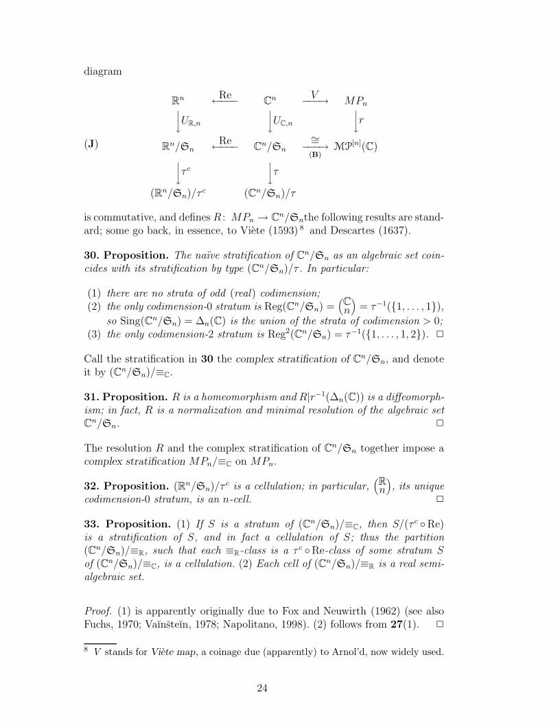
diagram

(J)

Rn Re←−−− Cn V

−−−→ MPnyUR,n

yUC,n

yr

Rn/SnRe←−−− Cn/Sn

∼=−−−→(B)

MP[n](C)

yτc

yτ

(Rn/Sn)/τ c (Cn/Sn)/τ

is commutative, and defines R : MPn → Cn/Snthe following results are stand-ard; some go back, in essence, to Viete (1593) 8 and Descartes (1637).

30. Proposition. The naıve stratification of Cn/Sn as an algebraic set coin-

cides with its stratification by type (Cn/Sn)/τ . In particular:

(1) there are no strata of odd (real) codimension;

(2) the only codimension-0 stratum is Reg(Cn/Sn) =(Cn

)= τ−1(1, . . . , 1),

so Sing(Cn/Sn) = ∆n(C) is the union of the strata of codimension > 0;(3) the only codimension-2 stratum is Reg2(Cn/Sn) = τ−1(1, . . . , 1, 2). 2

Call the stratification in 30 the complex stratification of Cn/Sn, and denoteit by (Cn/Sn)/≡C.

31. Proposition. R is a homeomorphism and R|r−1(∆n(C)) is a diffeomorph-

ism; in fact, R is a normalization and minimal resolution of the algebraic set

Cn/Sn. 2

The resolution R and the complex stratification of Cn/Sn together impose acomplex stratification MPn/≡C on MPn.

32. Proposition. (Rn/Sn)/τ c is a cellulation; in particular,(Rn

), its unique

codimension-0 stratum, is an n-cell. 2

33. Proposition. (1) If S is a stratum of (Cn/Sn)/≡C, then S/(τ c Re)is a stratification of S, and in fact a cellulation of S; thus the partition

(Cn/Sn)/≡R, such that each ≡R-class is a τ c Re-class of some stratum Sof (Cn/Sn)/≡C, is a cellulation. (2) Each cell of (Cn/Sn)/≡R is a real semi-

algebraic set.

Proof. (1) is apparently originally due to Fox and Neuwirth (1962) (see alsoFuchs, 1970; Vaınsteın, 1978; Napolitano, 1998). (2) follows from 27(1). 2

8 V stands for Viete map, a coinage due (apparently) to Arnol’d, now widely used.

24

Call the cellulation in 33 the real cellulation of Cn/Sn, and denote it by(Cn/Sn)/≡R. The resolution R and the real cellulation of Cn/Sn togetherimpose a real cellulation MPn/≡R on MPn. The real cellulations of Cn/Sn

and MPn in turn define real cellulations of MP[n](C), ∆n(C), R−1(MP

[n](C)),and R−1(∆n(C)).

34. Examples. For small n, very explicit descriptions of the complex strati-fications are easily given.

34.1. MP1/≡C consists of a single stratum, necessarily of codimension-0.

34.2. MP2/≡C consists of two incident strata: R−1((C2

)), of codimension 0, is

diffeomorphic to C×(C \ 0); R−1(∆2(C)), of codimension 2, is diffeomorphicto C. Explicitly, C2/S2 → C2 : w1, w2 7→ (w1 + w2, (w1 − w2)

2) is a

homeomorphism that maps(C2

)(resp., ∆2(C)) diffeomorphically onto C \ 0

(resp., C× 0).

34.3. MP3/≡C consists of three mutually incident strata:(C3

), of codimension

0, is diffeomorphic to C × (C2 \ Vf ), where f(z1, z2) = 4z31 + 9z2

2 and so Vf

is a cuspidal cubic curve, homeomorphic to C and having a single singularpoint; Reg(∆3(C)), of codimension 2, is diffeomorphic to C × Reg(Vf ) andtherefore to C×C \ 0; and Sing(∆3(C)), of codimension 4, is diffeomorphicto C × Sing(Vf ) and therefore to C. It is easy to write down an explicitpolynomial homeomorphism C3/S3 → C3 giving an isomorphic stratification.

The real cellulations of MPn, and thus of(Cn

)and ∆n(C), can be described

very explicitly, in all dimensions (see Fox and Neuwirth, 1962; Napolitano,2000). For the purposes of this survey, it is sufficient to describe the cells ofdimension 2n, 2n − 1, and 2n − 2 only, along with their incidence relations;this can be done in a uniform manner for all n.

35. Example. In(Cn

)/≡R there is exactly one cell of dimension 2n, exactly

n−1 cells of dimension 2n−1, and exactly (n−1)(n−2)/2 cells of dimension2n− 2.

(1) The cell C0 of dimension 2n consists of all z1, . . . , zn with Re z1 < · · · <Re zn.

(2) For k = 1, . . . , n − 1, there is a cell Ck of dimension 2n − 1 consistingof all z1, . . . , zn with Re z1 < · · · < Re zk = Re zk+1 < · · · < Re zn

and Im zk 6= Im zk+1; Ck is transversely oriented by the complex orienta-tion of MPn, and C0 is incident on Ck from both sides—more precisely,there is a simple closed curve in

(Cn

)that intersects Ck in a single point,

transversely, and is otherwise contained in C0.(3) For 1 ≤ k ≤ n−2, there is a cell Ck,k+1 of dimension 2n−2 consisting of allz1, . . . , zn with Re z1 < · · · < Re zk = Re zk+1 = Re zk+2 < · · · < Re zn

25

C0 C0 C0

C0 C0

Ck Cj

Ck

Ck

Ck+1

Ck+1

Ck+1 Cj

Ci

Ci Ck

C0 C0

C0

C0C0

C0 C0

= Ck,k+1 = Ci,j = Dk

Figure 14. The transverse structure of MPn/≡R along its codimension-2 cells.

and card() Im zk, Im zk+1, Im zk+2 = 3. The two cells Ck and Ck+1 ofdimension 2n− 1 are each triply incident on Ck,k+1—more precisely, thestratification induced on a small 2–disk in MPn intersecting Ck,k+1 in asingle point, transversely, is as pictured to the left of Figure 14.

(4) For 1 ≤ i < j − 1 ≤ n − 2, there is a cell Ci,j of dimension 2n − 2consisting of all z1, . . . , zn with Re z1 < · · · < Re zi = Re zi+1 < · · · <Re zj = Re zj+1 < · · · < Re zn, Im zi 6= Im zi+1, and Im zj 6= Im zj+1.The two cells Ci and Cj of dimension 2n − 1 are each doubly incidenton Ci,j—more precisely, the stratification induced on a small 2–disk inMPn intersecting Ci,j in a single point, transversely, is as pictured in themiddle of Figure 14.

In ∆n(C)/≡R, there are no cells of dimension 2n or 2n−1. For 1 ≤ k ≤ n−2,there is one cell Dk of dimension 2n − 2 consisting of all z1, . . . , zn withRe z1 < · · · < Re zk = Re zk+1 < · · · < Re zn and Im zk = Im zk+1. Thestratification induced on a small 2–disk in MPn intersecting Dk transverselyat a single point is as pictured at the right of Figure 14.

1.10 Contact 3-manifolds, Stein domains, and Stein surfaces

This section simply resumes basic definitions and needed results. For details oncontact structures and contact 3–manifolds, see Etnyre (this Handbook). Forthe topology of Stein domains and Stein surfaces, see Gompf (1998). For thecomplex function theory of Stein domains, Stein manifolds, and Stein spaces(in general dimensions), see Gunning and Rossi (1965).

36. Definitions. Let M be a 3–manifold without boundary. A contact struc-

ture on M is a completely non-integrable field ξ of tangent 2-planes on M ;for instance, on any round 3–sphere S3 ⊂ C2, the field ξ of tangent 2-planes that are actually complex lines is a contact structure, called the stand-

ard contact structure on that sphere. A 3–manifold with a contact struc-ture is called a contact manifold. A (closed) 1–submanifold L in a contact

26

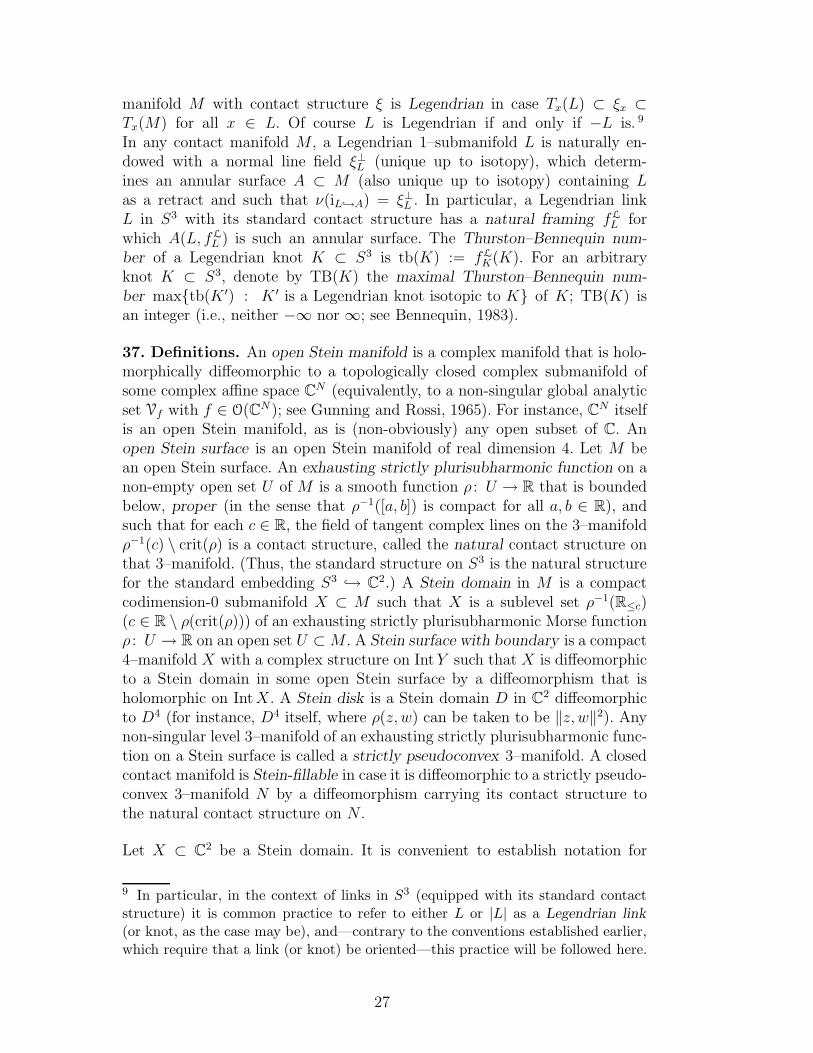
manifold M with contact structure ξ is Legendrian in case Tx(L) ⊂ ξx ⊂Tx(M) for all x ∈ L. Of course L is Legendrian if and only if −L is. 9

In any contact manifold M , a Legendrian 1–submanifold L is naturally en-dowed with a normal line field ξ⊥L (unique up to isotopy), which determ-ines an annular surface A ⊂ M (also unique up to isotopy) containing Las a retract and such that ν(iL→A) = ξ⊥L . In particular, a Legendrian linkL in S3 with its standard contact structure has a natural framing fL

L forwhich A(L, fL

L ) is such an annular surface. The Thurston–Bennequin num-

ber of a Legendrian knot K ⊂ S3 is tb(K) := fLK(K). For an arbitrary

knot K ⊂ S3, denote by TB(K) the maximal Thurston–Bennequin num-

ber maxtb(K ′) : K ′ is a Legendrian knot isotopic to K of K; TB(K) isan integer (i.e., neither −∞ nor ∞; see Bennequin, 1983).

37. Definitions. An open Stein manifold is a complex manifold that is holo-morphically diffeomorphic to a topologically closed complex submanifold ofsome complex affine space CN (equivalently, to a non-singular global analyticset Vf with f ∈ O(CN ); see Gunning and Rossi, 1965). For instance, CN itselfis an open Stein manifold, as is (non-obviously) any open subset of C. Anopen Stein surface is an open Stein manifold of real dimension 4. Let M bean open Stein surface. An exhausting strictly plurisubharmonic function on anon-empty open set U of M is a smooth function ρ : U → R that is boundedbelow, proper (in the sense that ρ−1([a, b]) is compact for all a, b ∈ R), andsuch that for each c ∈ R, the field of tangent complex lines on the 3–manifoldρ−1(c) \ crit(ρ) is a contact structure, called the natural contact structure onthat 3–manifold. (Thus, the standard structure on S3 is the natural structurefor the standard embedding S3 → C2.) A Stein domain in M is a compactcodimension-0 submanifold X ⊂ M such that X is a sublevel set ρ−1(R≤c)(c ∈ R \ ρ(crit(ρ))) of an exhausting strictly plurisubharmonic Morse functionρ : U → R on an open set U ⊂M . A Stein surface with boundary is a compact4–manifold X with a complex structure on IntY such that X is diffeomorphicto a Stein domain in some open Stein surface by a diffeomorphism that isholomorphic on IntX. A Stein disk is a Stein domain D in C2 diffeomorphicto D4 (for instance, D4 itself, where ρ(z, w) can be taken to be ‖z, w‖2). Anynon-singular level 3–manifold of an exhausting strictly plurisubharmonic func-tion on a Stein surface is called a strictly pseudoconvex 3–manifold. A closedcontact manifold is Stein-fillable in case it is diffeomorphic to a strictly pseudo-convex 3–manifold N by a diffeomorphism carrying its contact structure tothe natural contact structure on N .

Let X ⊂ C2 be a Stein domain. It is convenient to establish notation for

9 In particular, in the context of links in S3 (equipped with its standard contactstructure) it is common practice to refer to either L or |L| as a Legendrian link

(or knot, as the case may be), and—contrary to the conventions established earlier,which require that a link (or knot) be oriented—this practice will be followed here.

27

several subsets of C(X) := f : X → C : f is continuous; although C(X),equipped with its sup norm, is a well known Banach algebra, here it (and itssubsets) will not be endowed with any topology.

(K)

A(X) := f ∈ C(X) : f |IntX is holomorphic

O(X) := f ∈ C(X) : f = F |X for some open neighborhood U of

X in C2 and some holomorphic F : U → C

U(X) := f ∈ O(X) : 0 /∈ f(X)

W(X) := f ∈ O(X) : 0 /∈ f(IntX).

An element of A(X) is called a germ of a holomorphic function on X. BothA(X) and O(X) are algebras. By a standard argument, U(X) is the groupof units of O(X). Clearly W(X) is a multiplicative subsemigroup of O(X)properly containing U(X).

Major reasons for complex analysts’ interest in Stein manifolds include generaltheorems of which the following are special cases.

38. Theorem. If X ⊂ C2 is a Stein disk and Γ ⊂ U is a holomorphic curve

in an open neighborhood U of X, then Γ∩X = f−1(0) for some f ∈ O(X). 2

39. Theorem. Any holomorphic function on a Stein disk X can be arbitrarily

closely uniformly approximated, along with any finite number of its derivatives,

by the restriction to X of a polynomial function. 2

The following results are especially useful for topological applications.

40. Theorem. If X ⊂ C2 is a Stein disk with exhausting plurisubharmonic

Morse function ρ, and f ∈ O(X) is such that Sing(Vf ) = ∅, then Vf is

ρ-ribbon. 2

41. Theorem. Every covering space of an open Stein manifold is an open

Stein manifold. A finite-sheeted branched covering space of a Stein disk branched

along a non-singular holomorphic curve is a Stein surface with boundary. 2

28

2 Braids and braided surfaces

Much of the following material is treated (usually more generally and of-ten from a different perspective) by Birman (1975) and Birman and Brendle(this Handbook), references to which should be assumed throughout.

2.1 Braid groups

42. Definition. For any n ∈ N>0 and X ∈(Cn

), let BX := π1(

(Cn

);X), and

call BX an n-string braid group. 10 The standard n-string braid group is

Bn := Bn. By convention, the (unique) 0-string braid group is B0 := o.Write oX for the identity of BX , and let o(n) := on.

Of course, since(Cn

)is connected, every n-string braid group is isomorphic

to Bn, but it is very convenient to allow more general basepoints. With theconventions in 42, B0 is isomorphic but not identical to B1 = o(1); this isconsistent with the obvious fact that the groups Bn, n ∈ N>0, being funda-mental groups of pairwise distinct spaces, are pairwise disjoint.

43. Theorem.

(L) Bn = gp(σs, s ∈ 1, . . . , n− 1 :

[σs, σt] (|s− t| > 1),

≪ σs, σt ≫ (|s− t| = 1)

)2

It is usual to call (L) the standard presentation of Bn, the generators σs

of (L) the standard generators of Bn, and the relators of (L) the stand-

ard relators of Bn. (It is also usual, and perhaps regrettable, to conflateσs ∈ Bn with σs ∈ Bn′ for all n, n′ > s. A more precise notation wasproposed by Rudolph, 1985b, see 52.) The detailed proof of 43 given byFox and Neuwirth (1962) is, more or less exactly, an application of the usual al-gorithm (as in Magnus, Karrass, and Solitar, 1976), which produces a present-ation of the fundamental group of a 2-dimensional cell complex with one 0-cell(the basepoint) having a generator for each 1-cell and a relator for each 2-cell,

to the 2-skeleton of the cellulation of(Cn

)that is dual to

(Cn

)/≡R.

10 As Magnus (1974, 1976) points out, in effect π1((Cn)) was investigated, and re-

cognized as a “braid group”, by Hurwitz as early as 1891. Apparently this insighthad been long forgotten when Fox and Neuwirth (1962, p. 119) described as “previ-ously unnoted” their “remark that Bn may be considered as the fundamental groupof the space . . . of configurations of n undifferentiated points in the plane.” It isinteresting to speculate as to possible reasons for this instance of what Epple calls“elimination of contexts” (see especially Epple, 1995, p. 386, n. 32).

29

2.2 Geometric braids and closed braids

Let I ⊂ R be a closed interval. Let p : I →(Cn

)be a closed path. The

multigraph gr(p) ⊂ I × C of p is called a n-string geometric braid for the(algebraic) braid in Bp(∂I) represented by p.

Let q : O′ →(Cn

)be a loop with domain the horizontal unknot O′ ⊂ S3.

The multigraph gr(q) ⊂ S1 × C of q is a simple collection of closed curves inthe open solid torus O′ × C. Using the vertical unbook o, it is easy to createa (nearly standard) identification of O′ × C with S3 \O, and thus a (nearlystandard) embedding of gr(q) into S3 \O. This embedding has the propertythat arg(o)| gr(q) : gr(q)→ S1 is a covering map of degree n, and every simplecollection of closed curves L ⊂ O′×C such that arg(o)|L : L→ S1 is a coveringmap of degree n arises in this way from some q. Call any such L an n-stringclosed o-braid (Rudolph, 1988). In general, if a is an unbook (that is, an openbook on S3 with unknotted binding A), then a is equivalent to o, and the classof closed a-braids (sometimes called, slightly abusively, simply “closed braidswith axis A”) is defined by any such equivalence. Given a basepoint ∗ ∈ O′,q naturally represents an element of βq ∈ Bq(∗). The notation β(βq) is oftenused for the closed o-braid gr(q).

2.3 Bands and espaliers

For n = 2, (L) says that B2 is infinite cyclic. More specifically and directly,34(2) shows that, for any edge e ⊂ C, the 2-string braid group B∂e is infin-ite cyclic with a preferred generator, say σe; in fact σe depends only on ∂e.In particular, any two 2-string braid groups are canonically isomorphic. Forn > 2, typically no isomorphism between distinct n-string braid groups hasmuch claim to be called canonical; however, the following is an immediateconsequence of 32.

44. Proposition. If X ∈(Rn

), then BX

∼= Bn, and any path in(Rn

)from X

to n induces this canonical isomorphism. 2

For n ≥ 2, if X ∩ e = ∂e, then there is a natural injection ie;X : B∂e → BX ,and i∂e;X depends only on the isotopy class of e (rel. ∂e) in C \ (X \ e).

45. Definitions. A positive X-band is any σe;X := ie;X(σe) ∈ BX . (WhenX is understood, or irrelevant, σe;X may be abusively abbreviated to σe.) Anegative X-band is the inverse of a positive X-band. An X-band is a positiveor negative X-band. Let |σ±1

e;X | := σe;X denote the absolute value of the band

σ±1e;X , ε(σ±1

e;X) := ± the sign (positive or negative) of σ±1e;X , and e(σ±1

e;X) the

30

edge-class of σ±1e;X , that is, the isotopy class (rel. ∂e) of e in C \ (X \ e). An

X-bandword of length k is a k-tuple b =: (b(1), . . . , b(k)) such that each b(i) isan X-band. 11 An X-bandword b is quasipositive in case each b(i) is a positive

X-band. The braid of b is β(b) := b(1) · · · b(k) ∈ BX . Every braid in BX isthe braid of some X-bandword. A braid in BX is quasipositive in case it isthe braid of a quasipositive X-bandword.

Orevkov (2004) gives an algorithm to determine whether or not a given braidin B3 is quasipositive. Bentalha (2004) generalizes this to all Bn.

46. Proposition. Any two positive X-bands are conjugate in BX. 2

An n-string braid group is the knotgroup of ∆n(C) in(Cn

)(see Rudolph,

1983b); a positive band is a meridian.

47. Proposition. Let X ∈(Cn

), n ≥ 2. Let e, f ⊂ C be two edges with X∩e =

∂e, X∩f = ∂f . If e∩f = ∅ (resp., e∩f = x ⊂ ∂e∩∂f), then [σe;X , σf ;X ] = oX

(resp., ≪ σe;X , σf ;X ≫ = oX).

Proof. This is readily proved directly. Alternatively, note that: (1) the generalcase is isotopic to a special case in which X = n, e = [1, 2], and f = [s, s+ 1]with s ∈ 2, . . . , n; (2) in such a special case, BX = Bn, σe;X = σ1 andσf ;X = σs are two standard generators of (L), and the claimed commutatorand yangbaxter relators are two standard relators of (L). 2

48. Proposition. Let T ⊂ C be a planar tree. The positive V(T)-bands

σe;V(T), e ∈ E(T), generate BV(T); no proper subset of them does so. If e ∩f = ∅ (resp., e ∩ f = z, z ∈ V(T)), then [σe;V(T), σf ;V(T)] = oV(T) (resp.,≪σe;V(T), σf ;V(T) ≫ = oV(T)). 2

Call the V(T)-bands σe;V(T), e ∈ E(T), the T-generators of BV(T). Note that48 asserts that the braid group BV(T) is a quotient of

(M) gp(σe, e ∈ E(T) :

[σe, σf ] (card(e ∩ f) = 0),

≪σe, σf ≫ (card(e ∩ f) = 1)

)

but not that these groups are identical. In fact they are easily seen to be so ifand only if T has no intrinsic vertices.

An espalier is a planar tree T such that each e ∈ E(T) is a proper edge inC− and Re |(e \ Col(∂e ⊂ e)) is injective. Rudolph (2001a) gives proofs of thefollowing facts about espaliers.

11 In particular, n-bandwords are just what (since 1983a) I have long called “bandrepresentations”—a coinage which I would like to suppress, due to its misleadingsuggestion of a relation to group representation theory.

31

49. Proposition. (1) Every planar tree is isotopic, in C, to an espalier.

(2) The embedding of an espalier T in C− is determined, up to isotopy of

(T,V(T)) in (C−,R), by the combinatorial structure of its cellulation together

with the order induced on V(T) by its embedding in R = ∂C−. In particular,

given X = x1 < · · · < xn ⊂ R and n − 1 pairs xi(p) < xj(p) ⊂ X, the

following are equivalent. (a) There is an espalier T with V(T) = x1, . . . , xn,E(T) = e1, . . . , en−1, and ∂ep = xi(p), xj(p). (b) For 1 ≤ p < q ≤ n− 1 the

pairs xi(p) < xj(p) and xi(q) < xj(q) are not linked (i.e., they are either in

touch or unlinked). 2

50. Definition. Let X ∈(Rn

). An X-band σ is embedded provided that some

e ∈ e(σ) is a proper edge in C−; when it is given that σ = σ±1e;X is embedded,

it is assumed without further comment that e ∈ e(σ) is such an edge. Clearlythere are exactly n(n− 1)/2 embedded positive X-bands, one—which may bedenoted σxi,xj ;X—for each xi < xj ⊂ X. The embedded positive X-bandsgenerate BX . (A presentation (A) of Bn with the positive n-bands as gener-ators is given by Birman et al., 1998, and many interesting conclusions drawntherefrom.) An X-bandword b is embedded in case each b(i) is embedded. AnX-bandword b is called positive in case it is both quasipositive and embedded.

Let X0 ⊂ X ∈(Cn

). Unless n0 := card(X0) equals n, typically no non-trivial

homomorphism BX0 → BX has much claim to be called canonical. For X ⊂R, however, the situation is much better (cf. 44). In fact, given a positiveembedded X0-band σxi,xj ;X0 ∈ BX0 , let iX0;X(σxi,xj ;X0) := σxi,xj ;X ∈ BX .

51. Proposition. There is a unique homomorphism iX0;X : BX0 → BX ex-

tending iX0;X as defined on the embedded X0-bands, and it is injective. 2

Call iX0;X the canonical injection of BX0 into BX . (The collision of notationwith ie;X is unproblematic; if X ⊂ R and e is embedded with ∂e = xi, xj,then ixi,xj ;X = i∂e;X .) 51 excuses the conflation, under the single name σxi,xj

,of all the positive embedded bands σxi,xj ;X for ξi < ξj ⊂ X ⊂ R, X finite.

52. Example. For n ≥ m, the canonical injection im;n is implicit in the iden-tification of Bm as a subgroup of Bn, discussed following 43. Rudolph (1985b)proposed the notation β(n−m) for im;n(β), and the convention (extending thenotations o and o(n) introduced in 42) that for each m ∈ N, σm−1 denote only

an element of Bm, the other standard generators of Bm being σ(m−2)1 , . . . , σ

(1)m−2.

This notation and convention have been widely unadopted.

53. Definition. Let T be an espalier. A T-bandword is a V(T)-bandwordb such that every |b(i)| is a T-generator (so, in particular, a T-bandword isan embedded V(T)-bandword). A positive T-bandword b is called strictly T-

positive in case every T-generator appears among the bands b(s).

32

For X = x1 < · · · < xn ∈ MP[n](R), let IX (resp., YX) denote any espalier

T with V(T) = X and ∂e : e ∈ E(T) = xp, xp+1 : 1 ≤ p < n (resp.,x1, xp : 1 < p ≤ n). Among the combinatorial types of trees T withV(T) = X, IX and YX represent two extreme types, which may be called linear

(minimal number of endpoints) and star-like (maximal number of endpoints),respectively; further, among the linear (resp., star-like) espaliers, IX (resp.,YX) is again extreme, in a sense that is obvious and easily formalized.

54. Example. The In-generators of Bn are the standard generators of (L),an In-bandword is just a “braid word” in the usual sense (Birman, 1975, p. 70ff.), and the braid of an In-positive (or, for some authors, strictly In-positive)In-bandword is a “positive braid” in the usual sense (Birman, 1975; Rudolph,1982b; Franks and Williams, 1987, etc., etc.).

55. Question. As noted after 43, the standard generators and standard relat-ors of (L) correspond naturally to the codimension-1 and codimension-2 cells

of(Cn

)/≡R. As noted in 54, the standard generators also correspond naturally

to the edges of In. Clearly, given any linear planar tree T with card(V(T)) = n,

from an isotopy of T to In may be contrived a cellulation(Cn

)/≡T with a unique

codimension-0 cell, such that (1) the codimension-1 cells of(Cn

)/≡T corres-

pond to the T-generators of BV(T), and (2) the codimension-2 cells of(Cn

)/≡T

correspond to the relators of L. Now suppose that T is a planar tree for which

there exists a (natural or contrived) cellulation(Cn

)/≡T, with a unique codi-

mension-0 cell, that has property (1) but, rather than property (2), satisfies

both (3) some of the codimension-2 cells of(Cn

)/≡T correspond to the relators

of (M), and (4) the remaining codimension-2 cells of(Cn

)/≡T correspond to

some family of extra relators exactly sufficient to convert (M) into a presenta-tion of BV(T). Does this imply that, in fact, T is linear? Specifically, does there

exist a cellulation(C4

)/≡Y4

with properties (1), (3), and (4)?

The methods of Birman, Ko, and Lee (1998) might help answer 55 (althoughthe presentation they give is not obviously associated to a cellulation).

2.4 Embedded bandwords and braided Seifert surfaces

Early versions of the construction of braided Seifert surfaces described in thissection appeared in Rudolph (1983b,c).

56. Construction. Let X ∈(Rn

), T ∈

(Rk

), say X =: x1 < · · · < xn,

T =: t1 < · · · < tk. Let 0 < ǫ < min|t − t′|/2 : t, t′ ∈ T, t 6= t′; in case

33

k > 0, let I = [minT − ǫ,max T + ǫ]. Let b be an embedded X-bandword oflength k. To implement this construction of braided Seifert surfaces, choose aproper arc es ⊂ C− in the edge-class e(b(s)) for each s ∈ k, and embeddingsηx : h(0) → C+×R (x ∈ X) and η t : h(1) → C−× ]t− ǫ, t+ ǫ[ (t ∈ T ), subjectto the following conditions. For each x ∈ X,

(1) ηx is proper along a boundary arc of h(0),(2) ηx(h(0)) ⊂ x + iy : y ∈ R≥0 ×R,(3) and I ⊂ ∂ηx(h(0)).

For each t ∈ T , say t = tp, p ∈ k,

(4) η tp is proper along the attaching arcs of h(1),(5) pr1 η tp|κ(h(1)) : κ(h(1))→ C− is a diffeomorphism onto ep,(6) (Re pr1, pr2) η t : h(1) → R× R is a bowtie, and(7) the sign of the crossing of (Re pr1, pr2) η t|∂h

(1) is equal to ε(b(t)).

It follows that

(N) Σ(b) :=⋃

x∈X

ηx(h(0)) ∪⋃

t∈T

η t(h(1)) ⊂ C× R

is a (0, 1)-handle decomposition (C) of a surface. Any Seifert surface S[b] :=δ(Σ(b)) ⊂ R3 ⊂ S3, where δ : C×R→ R3 : (z, t) 7→ (Re z, Im z, t) and Σ(b)is constructed as in 56, is called a braided Seifert surface of the embeddedX-bandword b. It is easy to see that γ(b) := Σ(b) ∩ (C− × I) is a geometricbraid for β(b), and that the link ∂S[b] is isotopic in S3 ⊃ R3 to β(b).

The braid diagram of b is the pair BD(b) =: (P(BD(b)), I(BD(b))), whereP(BD(b)) := (Re, pr2)(γ(b)) ⊂ R×I and I(BD(b)) is the information aboutthe signs of the crossings of P(BD(b)) (indicated graphically in the style of11(2); see Figure 15). A braid diagram for β ∈ BX is a braid diagram of anybandword b with β(b) = β. A standard braid diagram for β ∈ Bn is a braiddiagram of any In-bandword b with β(b) = β.

Of course b determines S[b] and β(b) up to isotopy; and clearly, up to iso-topy (even isotopy through braided Seifert surfaces), none of X, T , or thecollection of specific edge-class representatives es is necessary per se to theconstruction of S[b]—all that is needed is a modicum of combinatorial inform-ation extracted from b. That information can be encoded as the k-tuple oftriples ((ib(1), jb(1), εb(1)), . . . , (ib(k), jb(k), εb(k))) with xib(s) < xjb(s) :=∂es ⊂ X and εb(s) := ε(b(s)). Another convenient encoding is graphical, us-ing charged fence diagrams (see Rudolph, 1992a, 1998). Figure 16 pictures a(very simple) charged fence diagram. 12

12 In Rudolph (1992a), I described fence diagrams as “my synthesis of some diagramsthat H. Morton used to describe certain Hopf-plumbed fiber surfaces in 1982 . . . and‘square bridge projections’ as described by H. Lyon” (Lyon, 1980). By 2001a, I hadrecalled that I first saw fences (and braid groups!) “c. 1959, in one of Martin Gard-

34

Figure 15. Left: a surface Σ(b); ε(b(1)) = −, ε(b(1)) = +. Right: a braid diagramfor β(b).

Figure 16. A charged fence diagram for the surface in Figure 15.

There is a more or less canonical way to turn an n-string braid diagram BD(b)into a standard link diagram D(β(b)): identify C with R2 ⊃ P(BD(b)) by(Re, Im); in C, attach n arcs to P(BD(b)) ⊂ C, preserving orientation, soas to create a normal collection P(D(β(b))) of closed curves with no newcrossings; and let I(D(β(b))) be I(BD(b)).

57. Proposition. (1) Let b be an In-bandword. Let L = β(b). The arcs

P(D(L)) \ Int P(BD(b)) can be chosen so that OD(L) = O+D(L); if they are,

then D(L) is nested and the diagrammatic Seifert surface S(D(L)) is isotopic

to S[b]. (2) Conversely, if D(L) is nested and OD(L) = O+D(L), then (up to

isotopy of P(D(L))) there exists an In-bandword b, n := card(OD(L)), such

that L = β(b) and S(D(L)) is isotopic to S[b]. (3) If b is an embedded

ner’s ‘Mathematical Games’ columns” (reprinted in Gardner, 1966, as Chapter 2,“Group Theory and Braids”). Since 2001 I have become aware of “amida-diagrams”(introduced by Yamamoto, 1978, precisely to construct certain special Seifert sur-faces) and “wiring diagrams” (cf. Cordovil and Fachada, 1995, and other literaturefrom the theory of line arrangements), both closely related to fences, as are (via theiressential identity with square bridge projections) the “barber-pole projections” at-tributed in Rudolph (1992a) to Thurston (unpublished), Erlandsson (1981), andKuhn (1984). Is this another instance of Epple’s “elimination of contexts”, or amere multiplication of contexts?

35

n-bandword but not an In-bandword, and L = β(b), then D(L) is nested but

χ(S(D(L))) < χ(S[b]), so S(D(L)) and S[b] are not diffeomorphic, let alone

isotopic. 2

57 shows that 25 is equivalent to the following.

58. Theorem. For all n, for all β ∈ Bn,

(P) ordv Pβ≥ e(β)− n+ 1,

where e : Bn → Z is abelianization (exponent sum). 2

Proofs of the following theorem apppear in Rudolph (1983b,c); it also followsfrom results of Bennequin (1983) on “Markov surfaces” (see Rudolph, 1985b).

59. Theorem. If S ⊂ R3 ⊂ S3 is a Seifert surface, then there exist X and

an embedded X-bandword b such that S is isotopic to S[b]. 2

60. Question. The braid index brin(L) of a link L is the minimum n ∈ N>0

such that L is isotopic to β(b) for some n-bandword b (which can, since itslength is not an issue, be taken to be embedded); see Birman and Brendle(this Handbook). Let the braided Seifert surface index of a Seifert surface Sbe the minimum n ∈ N>0 such that S is isotopic to S[b] for some embed-ded n-bandword b; by 59, this invariant of S is an integer. How can it becalculated or estimated? This question is the analogue for Seifert surfaces of“Open Problem 1” of Birman and Brendle (this Handbook), which asks howto calculate brin(L). Clearly the braided Seifert surface index of S is at leastas great as brin(∂S). Examples of Hirasawa and Stoimenow (2003) show thatthis inequality can be strict.

61. Definition. A Seifert surface S is quasipositive in case S is isotopic to a

braided Seifert surface S[b] for some positive X-bandword b. A link is strongly

quasipositive in case it has a quasipositive Seifert surface.

2.5 Plumbing and braided Seifert surfaces

Let X ∈(Rn

). For x ∈ X, write X≤x := X ∩R≤x, X≥x := X ∩R≥x.

62. Definitions. Let x ∈ X. Let b be an embedded X-bandword of lengthk. Let Tb;≤x := s ∈ k : b(s) ∈ iX≤x,X and Tb;≥x := s ∈ k : b(s) ∈ iX≥x,X;let k≤ := card(Tb;≤x), k≥ := card(Tb;≥x), so in every case k≤ + k≥ ≤ k. Incase k≤ + k≥ = k, say that b is deplumbed by x ∈ X. Writing Tb;≤x =:u1 < · · · < uk≤

, Tb;≥x =: v1 < · · · < vk≥, let b≤x := (b≤x(1), . . . , b≤x(k≤))

(resp., b≥x := (b≥x(1), . . . , b≥x(k≥))) be the embedded X≤x-bandword (resp.,

36

= *

Figure 17. An example of deplumbing.

X≥x-bandword) for which iX≤x,X)b≤x(s) = b(us) (resp., iX≥x,X)b≥x(t) = b(vt)).By construction 56, if b is deplumbed by x ∈ X, then Σ(b) = Σ(b≤x)∪Σ(b≥x)and Σ(b≤x) ∩ Σ(b≥x) = Σ(b ∩ C × x is a disk (in fact, a 0-handle of theconstructed (0, 1)-handle decompositions of Σ(b≤x) ∪ Σ(b≥x)); the situationis illustrated using fence diagrams in Figure 17. The inverse of this opera-tion, which combines two braided Seifert surfaces into one, braided Stallings

plumbing .

Although it appears to be a rather special case of Stallings plumbing , or Mur-

asugi sum, a geometric operation on Seifert surfaces that has been extens-ively studied (by Murasugi, 1963; Conway, 1970; Siebenmann, 1975; Stallings,1978; Gabai, 1983a,b, 1986, and many others; notations, definitions, and somehistory are given by Rudolph, 1998), braided Stallings plumbing is in factperfectly general, according to Rudolph (1998).

63. Theorem. Up to isotopy, every Murasugi sum S0 * S1 of Seifert surfaces

S0, S1 is a braided Stallings plumbing of braided Seifert surfaces. 2

2.6 Labyrinths, braided surfaces in bidisks, and braided ribbons

Let X be a topological space. Given f : X → MPn, let f : X × C → C :(x, w) 7→ f(x)(w), so that gr(R f) = f−1

(0) . Generally it can be a subtlematter to determine whether a map F : X×C→ C (with fibers of cardinalitybounded by n ∈ N) is f for some (continuous) f : X → MPn, but in case Fis known to be such, write f = F.

64. Definition. A map f : X →MPn is amazing provided that the partitionof M into connected components of inverse images f−1(C) of the various cellsC of MPn/≡R has some finite refinement that is a stratification of X. Alabyrinth for f is any such stratification.

65. Examples. Amazing maps have proved useful in several applications.

37

65.1. If F (z, w) := f0(z)wn+f1(z)wn−1+· · ·+fn(z) ∈ C[z, w] is a polynomial

in Weierstrass form, then F : C → MPC is (in effect) F considered as anelement of C[z][w] ∼= C[z, w], and is amazing. Classically, in this situation wis said to be the “n-valued algebraic function of z without poles” determinedby the algebraic curve VF (Bliss, 1933; Hansen, 1988), and a more or lesscanonical set of “branch cuts” for w can be extracted systematically from thelabyrinth of F. Rudolph (1983a) determined the topology of the labyrinth ofF in the case Fǫ(z, w) = (w − 1)(w − 2) · · · (w − n + 1)(w − z) + ǫ, first forǫ = 0, then for small ǫ 6= 0, and used it to give the first proof of 77.

65.2. The term labyrinth was introduced by Dung and Ha (1995), in theirstudy of line arrangements in C2. In a linear coordinate system chosen sothat no line in the arrangement is vertical, such an arrangement is VF , whereF (z, w) ∈ C[z, w] is a product of (unrepeated) factors w + az + b (as in (1),where F0 corresponds to an arrangement of n − 1 horizontal lines crossed bya single diagonal line). Again, F exists and is amazing. (See §6.4 for furtherreferences on arrangements.)

65.3. Orevkov (1988) made excellent use of the observation that, if V ⊂ C2 isboth a C-algebraic curve and a nodal surface, then, after an arbitrarily smalllinear change of coordinates in C2, V = VF where F ∈ C[z, w] is in Weierstrassform and the labyrinth of the amazing map F has a very special form. (See§6.2 for further discussion of this application.)

65.4. Orevkov (1996) developed the theory of labyrinths in careful detail,and applied it to the Jacobian Conjecture. (See §6.3).

Amazing maps, and the facts about the low-codimension cells of MPn/≡R

laid out in 35, together allow two closely related constructions—of braidedsurfaces in bidisks, and braided ribbons in D4—to be described and carriedout more precisely than in the original sources (Rudolph, 1983b, 1985b).

66. Proposition. Let M be a surface. If f : M → MPn is transverse to all

the cells of MPn/≡R, then f is amazing. More specifically, f has a labyrinth

M/≡ with the following properties.

(1) The union of the vertices and edges of M/≡ is a graph Λ(f) with no

vertex of degree d /∈ 1, 4, 6.(2) The association by f to each edge e of Λ(f) of a codimension-1 cell of

MPn/≡R endows e with (a) a natural transverse orientation (and there-

fore a natural orientation, so that e is naturally either a simple closed

curve or an arc) and (b) a clew σ(e) in the set σ1, . . . , σn−1 of stand-

ard generators of the presentation (L) of Bn.

(3) The association by f to each vertex x of Λ(f) of a codimension-2 cell

of MPn/≡R endows x with either (a) a standard relator of (L), in case

valΛ(f)(x) ∈ 4, 6, or (b) a trivial relator σ±1s σ∓1

s in case valΛ(f)(x) = 1.

38

σi+1

σi+1

σiσj

σj

σi

σi

σi σi σi

σi+1

(|i-j|>2)

Figure 18. Clews in the labyrinth of a MPn/≡R-transverse map on a surface.

(4) The clews (2b) are consistent with the relators (3) as pictured in Figure 18.(In each local picture, the mirror image of the illustrated situation is also

allowed, as is simultaneous reversal of all edge orientations.) 2

67. Construction. A braided surface of degree n in D2×C is Sf := f−1 (0),

where f : D2 → MPn is transverse to all the cells of MPn/≡R as in 66.

68. Proposition. A braided surface Sf inD2×C is a surface, and pr1 |S : S →D2 is a simple branched covering map branched over V(Λ(f)). 2

In these terms, various facts about the constructions in (Rudolph, 1983b,1985b) can be phrased as follows. Since any braided surface Sf is compact, itis actually contained in D2 × rD2 for some r; clearly only braided surfaces inD2×D2 need be considered. The obvious identification of S1×D2 ⊂ ∂(D2×D2)with Nb(O′ ⊂ S3) identifies the boundary of a braided surface Sf ∈ D

2 ×D2

with a 1–submanifold of Nb(O′ ⊂ S3), which is a closed n-string o-braidisotopic to some β(b) of length card(V(Λ(f))). The bandword b can be read offfrom the clews of Λ(f). In particular, β(b) is the ordered product of the clewson the (oriented) edges of Λ(f) that intersect S1. Every bandword determinesa braided surface which is unique up to isotopy (through braided surfaces).Rudolph (1983a) characterizes quasipositive braided surfaces as follows.

69. Theorem. A braided surface Sf , where f is holomorphic, determines a

quasipositive bandword. Any braided surface that determines a quasipositive

bandword is isotopic (through braided surfaces) to Sf with f a polynomial. 2

There is a straightforward way to “round the corners” of D2×D2 by a smooth-

ing D2×D2 → D4—that is, a homeomorphism which is a diffeomorphism offS1 × S1—so that a braided surface in D2 ×D2 is carried to a ribbon surfacein D4. The converse is also true (Rudolph, 1983b, 1985b).

70. Theorem. Up to isotopy, every ribbon surface in D4 is the image of a

braided surface in D2 ×D2 by a smoothing D2 ×D2 → D4. 2

71. Theorem. Let b be an embedded bandword. The ribbon surface S in D4

with ∂S = ∂S[b] ⊂ S3, produced by pushing IntS[b] into IntD4, is isotopic

39

to the ribbon surface which is the image of the braided surface in D2 × D2

determined by the bandword b. 2

72. Definitions. A node (resp., cusp) in an n-string braid group BX is thesquare (resp., cube) of a X-band. A nodeword (resp., cuspword) in BX is ak-tuple b =: (b(1), . . . , b(k)) such that each b(i) is a band or a node (resp., aband, a node, or a cusp) in BX .

The proof of 70 can be generalized (cf. Rudolph, 1983b) to show that every“nodal ribbon surface” in D4 can be realized, up to smoothing and isotopy,by a “nodal braided surface” in D2×D2. Orevkov (1998) proved an immensegeneralization of 69; the following special case of Orevkov’s result is easy tostate and more than adequate for this review.

73. Theorem. If b is a quasipositive cuspword in Bn, then there is a holo-

morphic cusp curve in D2 × D2 that corresponds to b via an appropriate

holomorphic map f : D2 →MPn. 2

The map f in 73 is amazing; it is transverse to all the cells of MPn/≡R if andonly if the cuspword b is a bandword.

40

3 Transverse C-links

74. Definition. A link L ⊂ S3 is a transverse C-link provided that (S3, L)is diffeomorphic to (Σ,Vf ∩ Σ), where: (1) D ⊂ C2 is a Stein disk boundedby a strictly pseudoconvex 3–sphere Σ, and (2) f ∈ O(D) is a holomorphicfunction with Sing(Vf)∩Σ = ∅, such that (3) the complex manifold Reg(Vf )intersects Σ transversely and (4) Vf ∩Σ is non-empty (and therefore a smooth,naturally oriented closed 1–submanifold of Σ).

Various modifications may be made to the specifications in 74 without chan-ging the class of links so specified.

75. Proposition. (1) The requirement that Σ be strictly pseudoconvex can

be somewhat relaxed. (2) The requirement that Σ be strictly pseudoconvex can

be considerably strengthened: Σ can be required to be convex, or even to be a

round sphere. (3) Vf can be required to be non-singular, to be algebraic, or to

be both at once.

Proof (sketches). (1) Here, no attempt will be made to state the most generaltheorem (see 76(2)). A sufficient example for present purposes is the following.Let γ ⊂ C be an arbitrary simple closed curve and G ⊂ C the 2–disk that itbounds, so that for any r > 0 the bicylinder D := G × rD2 is diffeomorphic(indeed, biholomorphic) to the bidisk D1,1. Although D is not a Stein domain,IntD is an open Stein manifold, and (D, ∂D) can be arbitrarily closely ap-proximated by Stein domains. The result follows from 39 and transversality.(2) As pointed out by Boileau and Orevkov (2001), theorems of Eliashberg(1990) show that for this purpose all Stein disks are equally good. (3) Anearby level set of f will have no singularities and give the same link type; by39, f is arbitrarily closely approximated by its sufficiently high-degree Taylorpolynomials, and again we get the same link type. 2

76. Questions. 74 and 75 immediately suggest a number of questions.

76.1. Is there an algorithm for determining whether or not a given link isa transverse C-link? (It follows from 77 that the set of isotopy classes oftransverse C-links is recursive: there exists an algorithm that produces a linkin every such isotopy class. Thus the question becomes: Is the set of isotopyclasses of transverse C-links recursively enumerable?)

76.2. How much can the requirement that Σ be strictly pseudoconvex berelaxed (as in 75(1))? See Rudolph (1985a) for a cautionary result.

76.3. Let L be a transverse C-link. By 75(3), up to isotopy L = S3 ∩ Vf

for some f ∈ C[z, w]. What is the minimum degree of such a polynomial f?

41

In light of 75(2), the same question can be asked with the roundness of S3

weakened to convexity or strict pseudoconvexity of a 3–sphere Σ. Can either ofthese weakenings strictly decrease the minimum? Calculations of, or even goodupper bounds for, this (or these) invariant(s) of L would have applications tofinding embeddings of certain Stein domains (namely, cyclic branched covers ofD4 branched over holomorphic curves) into algebraic surfaces of unexpectedlylow degree in C3 (Boileau and Rudolph, 1995).

3.1 Transverse C-links are the same as quasipositive links

77. Theorem. Every quasipositive link is a transverse C-link. 2

Proofs of 77 (with some variation in the details) are presented in (Rudolph,1983a, 1984, 1985b). A remarkable theorem of Boileau and Orevkov (2001)asserts the converse.

78. Theorem. Every transverse C-link is a quasipositive link. 2

79. Corollary. L is a transverse C-link if and only if L is quasipositive. 2

80. Corollary. Every isotopy class of transverse C-links is represented by a

transverse intersection Vf ∩ (z, w) ∈ C2 : ‖(z, w)‖ = 1, where f ∈ C[z, w]and Sing(Vf) = ∅. 2

As Boileau and Orevkov note, their proof (the only one known to date) is com-pletely non-constructive, relying strongly as it does on the theory of pseudo-holomorphic curves (Gromov, 1985).

81. Question. Is there a constructive proof of 78? Biding such a proof, canan upper bound on n : L is isotopic to a quasipositive n-string braid bededuced from other invariants of a transverse C-link L?

3.2 Slice genus and unknotting number of transverse C-links

82. Theorem. If f ∈ O(D4) is such that Sing(Vf ) = ∅, and L is the trans-

verse C-link Vf ∩ S3, then Xs(L) = χ(Vf ∩D

4). 2

83. Corollary. If b is a quasipositive n-string bandword of length k, then

Xs(β(b)) = n− k. 2

It had been known at least as early as 1982 (Boileau and Weber, 1983; Rudolph,1983d) that these results would follow from a local version of the Thom Con-jecture (see A.6): either (in the case of 82) that L be a torus link On, n for

42

some n ∈ N>0, or (in the case of 83) that b be the important In-bandword 13

(Q) (

n repetitions︷ ︸︸ ︷σ1, σ2, . . . , σn−1, . . . , σ1, σ2, . . . , σn−1) =: ∇n

with closed braid β(∇n) = On, n. The first proof of the local Thom Conjec-ture was given by Kronheimer and Mrowka (1993), using gauge theory forembedded surfaces, a 4-dimensional technique. The full Thom Conjecture(and more) was proved using Seiberg–Witten theory—also a 4-dimensionaltechnique—by Kronheimer and Mrowka (1994); Morgan, Szabo, and Taubes(1996). Recently Rasmussen (2004) announced a purely 3-dimensional com-binatorial proof based on Khovanov homology.

84. Corollary. If L is a transverse C-link then Xr(L) = Xs(L). 2

It was also known (Boileau and Weber, 1983; Rudolph, 1983d) that the truthof the local Thom Conjecture implies an affirmative answer to “Milnor’s Ques-tion” (see A.5) on unknotting numbers of links of singularities (§4.1) or—moregenerally (see Rudolph, 1983b)—closed positive braids in the sense of 54.

85. Corollary. If L is the link of a singularity (e.g., a torus link Om,nwith 0 ≤ m < n), then u(L) = node(L) = (card(π0(L))−X(L))/2. 2

3.3 Strongly quasipositive links

82–85 immediately imply the following.

86. Theorem. If L is a strongly quasipositive link with quasipositive Seifert

surface S, then χ(S) = X(L) = Xr(L) = Xs(L). If K is a strongly quasipos-

itive knot with quasipositive Seifert surface S, then g(S) = g(K) = gr(K) =gs(K) ≤ node(K) ≤ u(K). 2

To fully exploit 86 it is necessary to have a good supply of transverse C-linksor, equivalently, quasipositive (closed) braids. Clearly every strongly quasipos-itive link (61) is quasipositive. The converse is false; for instance, the closed

13 There is a long and worthy tradition of designating (the braid of) thisIn-bandword as ∆2 (Birman, 1975; Birman and Brendle, this Handbook, etc., etc.),a usage apparently introduced by Fadell (1962) in homage to P. A. M. Dirac (whowrote that he “first thought of the string problem about 1929” in a letter quoted byGardner, 1966, addendum to Chapter 2; see also Newman, 1942). Nonetheless, inthe context of the knot theory of complex plane curves, where discriminants (whichhave their own, algebro-geometric, traditional claim on the notation ∆) abound, Ibelieve that the makeshift of using ∇ to stand in for ∆2 is preferable to the furtheroverloading of the symbol ∆.

43

Figure 19. “Trefoil insertion” on a fence diagram preserves the Seifert form whileeliminating a negative band.

braid of σ32σ1σ1 ∈ B3 is a quasipositive knot, but not strongly quasipositive

(by 83). Nonetheless, the class of strongly quasipositive links is very varied.

3.3.1 S-equivalence and strong quasipositivity

87. Proposition. No link invariant calculable from a Seifert matrix (for in-

stance, the Alexander polynomial of a knot, the signatures of a knot or link,

etc., etc.) can tell whether or not a link is quasipositive.

Proof. Let [(Li, Lj)S] be a Seifert matrix for a link L with Seifert surfaceS. By 59, we may assume that S = S[b], for some embedded X-bandwordb of length k. Let there be m ≤ k negative bands in b. If m = 0, we aredone. Otherwise, let b(s) be negative, say b(s) = σ−1

xp,xq, with xp < xq ⊂ X.

Let X ′ := X ∪ x′1, x′2, x

′3, x

′4, where xp < x′1 < x′2 < x′3 < x′4 < xq. Let

b′(t) = iX,X′b(t) for 1 ≤ t < s, b′(s) = σx′3,xq

, b′(s + 1) = σx′2,x′

4, b′(s + 2) =

σx′1,x′

3, b′(s + 3) = σxp,x2, b

′(s + 4) = σx′1,x′

4, and b′(t) = iX,X′b(t + 4) for

s + 4 < t ≤ k + 4 (see Figure 19 for a rendition of this operation in terms offence diagrams). Manifestly S[b] is diffeomorphic to S[b′] by a diffeomorphismthat is the identity of a single 1-handle, and an easy calculation shows thatthey have identical Seifert matrices. There are only m − 1 negative bands inb′, so this result of Rudolph (1983c) is true by induction on m. 2

88. Corollary. (1) Every S-equivalence class of knots contains strongly qua-

sipositive knots. (2) Every knot can be converted to a strongly quasipositive

knot by a sequence of “doubled-delta moves”.

Proof. Knots K0 and K1 are S-equivalent (in the first instance, Trotter, 1962,“h-equivalent”) just in case Ki has a Seifert surface Si such that some homo-logy bases of S0 and S1 produce identical Seifert matrices; so (1) is immediatefrom (the proof of) 87. Naik and Stanford (2003) introduced the “doubled-delta move”, an operation on standard link diagrams illustrated in Figure 20,and proved that the equivalence relation on knots generated by applying suchmoves is precisely S-equivalence; (2) follows directly. 2

89. Question. Conway (1970) introduced an operation on knots and linkscalled mutation. The result L′ of applying mutation to a link L is called a

44

Figure 20. The “doubled-delta” move.

mutant of L. Although mutant links can be non-isotopic, they are indistin-guishable by a wide variety of link invariants. Mutation was generalized byAnstee, Przytycki, and Rolfsen (1989). The result L′ of applying the opera-tion defined by Anstee, Przytycki, and Rolfsen to L is called a rotant of L.The doubled-delta move is a special case of Anstee, Przytycki, and Rolfsen’soperation. Obviously 88(2) can be rephrased as “the doubled-delta move neednot preserve strong quasipositivity”. In what circumstances is a rotant of astrongly quasipositive link strongly quasipositive? In particular, is a mutantof a strongly quasipositive link necessarily strongly quasipositive?

3.3.2 Characterization of strongly quasipositive links

There is a simple characterization of quasipositive Seifert surfaces, and thus—in some sense—of strongly quasipositive links.

90. Theorem. A Seifert surface S is quasipositive if and only if, for some

n ∈ N>0, S is ambient isotopic to a full subsurface of the fiber surface of the

torus link On, n. 2

91. Questions. Does there exist an algorithm to determine whether or nota given Seifert surface is quasipositive? Does there exist an algorithm to de-termine whether a given link is strongly quasipositive?

3.3.3 Quasipositive annuli

92. Lemma. Let (L, g) be a framed link such that the annular Seifert surface

A(L, g) is quasipositive. If the framing f of L is less twisted than g, then

A(L, f) is quasipositive.

Proof. This is the “Twist Insertion Lemma” of Rudolph (1983a) (with the signconventions in force here, it should be called the “Twist Reduction Lemma”).A proof using fence diagrams is shown in Figure 21. 2

45

Figure 21. “Twist reduction” on a fence diagram.

93. Definition. The modulus of quasipositivity of a knot K is

(R) q(K) := supt ∈ Z : A(K, t) is a quasipositive Seifert surface.

Rudolph (1990) applied 58 (via 26) and 90 to deduce the following.

94. Proposition. If A(L, f) is quasipositive, then ordvL, f ≥ 0. 2

95. Corollary. If K is a knot, then q(K) ≤ 12

ordvK ≤ −1−dega F∗K(a, x).

2

96. Corollary. If K is a knot, then q(K) ∈ Z. 2

Since q(K) = TB(K) (Rudolph, 1995), 96 also follows from Bennequin (1983).

97. Corollary. q(O) = −1. 2

98. Proposition. For K 6= O, q(K) = supf ∈ Z : the framed knot (K, f)embeds on the fiber surface of On, n for some n ∈ N>0.

Proof. If a framed knot (K, f) embedded on a Seifert surface S and K is notfull on S, then (K, f) = (O, 0); so 98 follows immediately from the character-ization theorem 90. 2

99. Corollary. A quasipositive Seifert surface is incompressible. 2

Of course 99 also follows from 85. Yet another proof can be extracted fromBennequin (1983).

3.3.4 Quasipositive plumbing

A somewhat lengthy but straightforward combinatorial proof of the followingtheorem appears in Rudolph (1998).

100. Theorem. A Murasugi sum is quasipositive if and only if its summands

are quasipositive. 2

46

101. Corollary. Iterated Murasugi sums of quasipositive annuli are quasipos-

itive Seifert surfaces. 2

102. Examples. 101 covers a surprising amount of ground.

102.1. A positive Hopf-plumbed fiber surface is an iterated Murasugi sum ofpositive Hopf annuli A(O,−1) starting from the trivial Murasugi sum D2. Afiber surface S is stably positive Hopf-plumbed in case some positive Hopf-plumbed fiber surface F can also be constructed as an iterated Murasugi sumof positive Hopf annuli A(O,−1) starting from S. A remarkable theorem ofGiroux (2002) states that a fibered link L has a stably positive Hopf-plumbedfiber surface if and only if a certain contact structure on S3 (constructedfrom the fibration in a way he describes) is the standard contact structure. Incombination with 90 and 100, Giroux’s theorem implies that a fibered link isstrongly quasipositive if and only if it is stably positive Hopf-plumbed.

102.2. A basket is a Seifert surface produced by repeatedly plumbing unknot-ted annuli A(O, ki) to a single fixed D2 ⊂ S3. (See Rudolph, 2001a, for detailsand examples.) A fundamental theorem of Gabai (1983b, 1985) implies thata basket is a fiber surface if and only if it is Hopf-plumbed (allowing bothpositive and negative Hopf annuli as plumbands). In particular, according toRudolph (2001a), a fiber surface is a quasipositive basket if and only if itis isotopic to a braided Seifert surface S[b] where b is a strictly T-positiveT-bandword for some espalier T.

102.3. General arborescent links are constructed as boundaries of unori-ented (possibly non-orientable) 2–manifolds formed by unoriented plumbing ,in which not just unknotted annuli A(O, ki) but also unknotted Mobius bandsare used as building blocks, while their mode of assembly is suitably restric-ted (it is coded by a planar tree with integer weights; see Conway, 1970;Siebenmann, 1975; Gabai, 1986). So-called special arborescent links (Sakuma,1994) are those obtained by disallowing Mobius plumbands. As noted byRudolph (2001a), the surfaces defining special arborescent links are baskets; inparticular, when all weights of an arborescent presentation of an arborescentlink L are strictly negative even integers, then L is strongly quasipositive.

102.4. The positively-clasped, k-twisted Whitehead double D(K; k; +) of aknot K is defined to be the boundary of the non-trivial plumbing (that is, nota boundary-connected sum) of A(K, k) and A(O,−1) (Figure 22 illustratesthis operation with a fence diagram). By 101 and 90, D(K; k; +) is stronglyquasipositive if and only if k ≤ TB(K) (see Rudolph, 1993).

102.5. If a set of Seifert surfaces contains A(O,−1) and is closed under iso-topy, Murasugi sum, and the operation of passing from a surface to a fullsubsurface, then it contains all quasipositive Seifert surfaces; and the set ofall quasipositive Seifert surfaces is the smallest set with these properties.

47

Figure 22. A fence diagram for the plumbed Seifert surface of D(O2, 3; 0;+).

3.3.5 Positive links are strongly quasipositive

A standard link diagram D(L) is called positive in case every crossing x ∈XD(L) is positive; a link L is positive if L has a positive standard link dia-gram. Nakamura (1998, 2000) and Rudolph (1999) independently proved thefollowing.

103. Theorem. If the standard link diagram D(L) is positive, then the dia-

grammatic Seifert surface S(D(L)) is quasipositive. 2

104. Corollary. A positive link is strongly quasipositive. 2

105. Questions. Two questions posed by Rudolph (1999) remain open andare relevant here.

105.1. Can positive links be characterized as strongly quasipositive links thatsatisfy some extra geometric conditions?

105.2. Does K ≥ O2, 3 imply that K is strongly quasipositive? (Here K1 ≥K2 means that K1 is concordant to K2 inside a 4-manifold with positive inter-section form; this partial order was defined and studied by Cochran and Gompf(1988), who showed that if K is a positive knot, then K ≥ O2, 3.)

3.3.6 Quasipositive pretzels

Braidzels are generalizations of the well-known (oriented) pretzel surfaces,with braiding data supplementing the twisting data that specifies an ordin-ary pretzel surface (a braidzel with trivial braiding); two typical pretzel sur-faces and two typical braidzel surfaces are pictured in Figure 23. Braidzelswere defined by Rudolph (2001b) and have been further studied by Nakamura(2004), who showed that every link has a Seifert surface which is a braidzel.Using braidzels, Rudolph (2001b) proved the following.

106. Proposition. The oriented pretzel surface P(t1, . . . , tk) is quasipositive

if and only if the even integer ti + tj is less than 0 for 1 ≤ i < j ≤ k. 2

48

Figure 23. The quasipositive pretzel surfaces P(4, 4,−2) and P(5, 5,−3); thebraidzel surfaces P(σ1, σ2

−1, σ1, σ2−1; 4, 4,−2) and P(σ2

−1, σ1, σ2−1, σ1; 1,−3,−3).

The question 89 was somewhat motivated by 106, since up to repeated muta-tion the pretzel link ∂P(t1, . . . , tk) depends only on t1, . . . , tk.

107. Question. What are necessary and sufficient conditions on the definingdata of a braidzel that it be quasipositive?

3.3.7 Links of divides

Identify C2 with the tangent bundle of C. A’Campo (1998) calls a normalcollection P of edges in D2 a divide, and constructs the link of the divide Pas L(P ) := (z, w) ∈ S3 : z ∈ P,w ∈ Tz(P ). This construction has beenextended—first by allowing non-proper edges (“free divides”; Gibson and Ishikawa,2002a), more generally by allowing immersed unoriented circle components(Kawamura, 2002), and more generally yet (and most recently) by allowingimmersions of graphs that are not 1–manifolds (“graph divides”; Kawamura,2004).

108. Theorem. If P is a divide, then: (1) L(P ) is fibered, and every link

L of a singularity is of the form L(P ) for some divide P (A’Campo, 1998);(2) L(P ) is strongly quasipositive (Hirasawa, 2000); (3) L(P ) is stably positive

Hopf-plumbed (Hirasawa, 2002); and indeed (4) L(P ) is positive Hopf-plumbed

(Ishikawa, 2002). If P is a free divide, possibly with circle components, then

(5) L(P ) is strongly quasipositive (Kawamura, 2002). If P is a graph divide,

then (6) L(P ) is quasipositive (Kawamura, 2004). 2

See also Couture and Perron (2000); Hongler and Weber (2000); Ishikawa (2001);Gibson and Ishikawa (2002b); Gibson (2002); Goda, Hirasawa, and Yamada(2002); Chmutov (2003).

49

Figure 24. A quasipositive fibered link which is not strongly quasipositive.

0

−3

3

−2

Figure 25. Two representations of a quasipositive Lover’s Knot.

3.4 Non-strongly quasipositive links

Other than the tautologous construction by forming the closed braid of aquasipositive braid, little is yet known about systematic constructions of non-strongly quasipositive transverse C-links.

109. Example. There exist fibered links which are quasipositive but notstrongly quasipositive (compare with 1). Examples include all the linksHn+m,m

obtained from On + 2m,n + 2m (m,n ≥ 1) by reversing the orientationof (any) m components. Figure 24 pictures a ribbon surface R = f(S1 ×[0, 1]

∐D2) for H1,1 and a fence diagram for the fiber surface sm(R) of H1,1.

110. Example. There exist arborescent links which are quasipositive but arenot special arborescent and not strongly quasipositive (compare with 3). Anexample is the quasipositive arborescent ribbon knot pictured, along with itsdefining weighted tree, in Figure 25.

111. Question. Every pretzel link is arborescent. (Caution: this does notmean that every pretzel link bounds an oriented pretzel surface, and in factthere is a natural sense in which those which do are a small minority. Nor isa typical oriented pretzel surface itself an arborescent Seifert surface.) Whatare necessary and sufficient conditions on an arborescent link that it be qua-sipositive, or strongly quasipositive?

Besides 106, some partial but systematic progress towards answering thisquestion has been made by Tanaka (1998) (for the of rational links).

50

4 Complex plane curves in the small and in the large

As noted in 80, every transverse C-link L is “algebraic” in the sense that, up toisotopy, L is the transverse intersection of rS3 = (z, w) ∈ C2 : ‖(z, w)‖ = rand a complex algebraic curve Vf ; clearly the same class of links arises whetherr > 0 is fixed once for all, or allowed to vary throughout R>0, so long asf is allowed to vary throughout C[z, w]. By contrast, interesting additionalrestrictions on the isotopy type of L arise in case, for each fixed Vf , r isconstrained to be either “very small” or “very large”. More precisely, thesituation is as follows (essentially this is proved by Milnor, 1968, in generaldimensions). Let F ∈ C[z, w] be non-constant and without repeated factors.The argument of F is F/|F | : C2 \ VF → S1. The Milnor map of F is isϕF := arg(()F )|(S2n−1 \ D(F )); for r > 0, the Milnor map of F at radius r,denoted by ϕF,r, is the Milnor map of (z, w) 7→ F (z/r, w/r). Let m(F ) :=inf‖(z, w)‖2 : F (z, w) = 0 = supr : rS3 ∩ VF = ∅.

112. Proposition. There is a finite set X(F ) ⊂ R>m(F ) of radii r with the fol-

lowing properties. (1) If r ∈ R>m(F ) \X(F ), then VF intersects rS3 transvers-

ally, so that L(F, r) := (1/r)(VF∩rS3) is a link in S3. (2) If r and r′ are in the

same component of R>m(F ) \ X(F ) then L(F, r) and L(F, r′) are isotopic. (3) If

m(F ) < r /∈ X(F ), then there is a trivialization n : L(F, r)×C→ ν(L(F, r)),as in 18, that lies in the homotopy class corresponding to any Seifert sur-

face for L(F, r) and such that ϕF,r is adapted to ϕF,r with d(K) = 1 for all

K ∈ π0(L(F, r)). 2

113. Definitions. In case F (0, 0) = 0, for any r ∈ ]0, m(F )[ the transverseC-link L(F, r) is called the link of the singularity of F (or of VF ) at (0, 0). Inany case, for any r > max X(F ) the transverse C-link L(F, r) is called the link

at infinity of F (or of VF ).

4.1 Links of singularities as transverse C-links

It can happen that ϕF,r has degenerate critical points, and so is not a Morsemap, or that ϕF,r is a Morse map but not a fibration (the latter in fact beingcommon: as noted in the first paragraph of this section, every transverse C-linkcan be realized as L(F, r) for some F and r > 0, while according to the previoussection many, many transverse C-links are not fibered links). However, Milnor(1968) proved the following (and its analogue in higher dimensions).

114. Theorem. If m(F ) < r < min X(F ), then L(F, r) is a fibered link and

ϕF,r is a fibration. 2

In other words, if L is a link of a singularity, then L is fibered.

51

Let L be the link of a singularity. There is a huge literature devoted to studyingthe algebraic and geometric topology L, and especially of its fibration (which,at the geometric level, completely determines L and all its invariants—thoughnot necessarily in a perspicuous fashion). Some starting points for the ded-icated reader are Eisenbud and Neumann (1985); Durfee (1999); Neumann(2001); Le Dung Trang (2003). Here it may simply be noted that many—though certainly not all—of the interesting topological features of the fibrationof L can profitably be explored using one or another of the representations of Lalluded to in earlier sections. On one hand, L is the link of a divide (A’Campo,1998), from which one representation of L as a positive Hopf-plumbed link canbe derived and exploited (A’Campo, 1998). On the other hand, it is easy touse labyrinths to see that L is a positive closed braid (and not overwhelm-ingly difficult actually to derive a specific positive braidword for L), whenceby Rudolph (2001a) one may derive (and, at least potentially, exploit) anapparently different—though surely closely related—representation of L as apositive Hopf-plumbed link.

4.2 Links at infinity as transverse C-links

Let L be a link at infinity. In general, L need not be fibered (for instance, everyunlink O(n) is a link at infinity, but only O = O(n) is fibered), but as Neumann(1989) puts it, L is “nearly” fibered. The literature on links at infinity is smallerthan that on links of singularities, but still too large and multifaceted to sum-marize here. The reader is referred to Boileau and Fourrier (1998) for a reviewup to 1998. Some more recent articles on various aspects of the subject areBodin (1999); Nemethi (1999); Neumann (1999); Bartolo and Cassou-Nogues(2000); Neumann and Norbury (2000); Paunescu and Zaharia (2000); Gwozdziewicz and P loski(2001, 2002); Rudolph (2002); Neumann and Norbury (2003); Cimasoni (2004).

52

5 Totally tangential C-links

115. Definition. A link L ⊂ S3 is a totally tangential C-link provided thatL = Vg ∩ S

3, where g ∈ O(C2) is such that Vg ∩ IntD4 = ∅ and Vg ∩ S3 is

a non-empty non-degenerate critical manifold of index 1 of ρ|Reg(Vg), withρ(z, w) := ‖(z, w)‖2.

This section follows Rudolph (1992b, 1995, 1997).

116. Lemma. L is a totally tangential C- if and only if (1) L is Legendrian

with respect to the standard contact structure on S3, and (2) L is an R-analytic

submanifold of S3. 2

By 116, a totally tangential C-link has a natural framing f = fLL .

117. Proposition. Let ρ : U → R be an exhausting strictly plurisubharmonic

function on an open set U ⊂ C2 such that D = ρ−1(R≤1) is a Stein disk, so

Σ := ∂D is a strictly pseudoconvex 3–sphere with a natural contact structure.

If g ∈W(D) ⊂ O(U) is such that Vg∩Σ is a non-empty non-degenerate critical

manifold M of index 1 of ρ|Reg(Vg), then M is a Legendrian 1–submanifold of

the contact manifold Σ. Further, there exists a totally tangential C-link L ⊂ S3

such that (Σ,M) is diffeomorphic to (S3, L) by a diffeomorphism carrying the

natural normal line field of M in Σ to the natural normal line field of L in

S3. 2

118. Question. Does every totally tangential C-link arise (up to isotopy) asin 115 with g required to be a polynomial? (Rudolph, 1995, shows that g maybe be required to be entire.)

119. Theorem. If L ⊂ S3 is Legendrian, then L is isotopic through Le-

gendrian links to a totally tangential C-link L′ with tb(L′) = tb(L).

Proof. The proof for knots (Rudolph, 1995) extends directly to links. 2

120. Corollary. If L ⊂ S3 is Legendrian, then there is a polynomial map

p : C2 → C such that (1) Sing(Vp) = ∅, (2) Vp intersects S3 transversely,

(3) Vp ∩D4 is an annular surface, and (4) Vp ∩ S

3 = ∂A(L, tbL). 2

Coupled with 82–85, the connection 120 between totally tangential C-linksand transverse C-links, leads to several interesting conclusions.

121. Theorem. If TB(K) ≥ 0, then K is not slice. 2

A front (see Eliashberg, 1993; Etnyre, this Handbook) is a piecewise-smoothlyimmersed curve γ ⊂ R2 of the sort illustrated in Figreffront figure: γ has

53

Figure 26. A front.

finitely many cuspidal corners and finitely many normal crossings; the cornersare exactly the local extrema of pr2 |γ; at a corner, the common tangent lineof the two branches is parallel to 0 × R; and elsewhere the tangent linesare parallel neither to 0 × R nor to R × 0. A front diagram is a pairFD(L) =: (P(FD(L)), I(FD(L))), where P(FD(L)) is a front, and I(D(L))is the information that L is a closed Legendrian 1–submanifold of R3 equippedwith a certain standard contact structure (consistent with its embedding asthe complement of a point in S3 equipped with its standard contact structure).

122. Lemma. (1) Given any front P(FD(L)), the information I(D(L)) is

true, and FD(L) determines |L| up to a vertical translation in R3. (2) A

standard link diagram D(L) for L can be derived from P(FD(L)) by (a) letting

P(D(L)) be P(FD(L)) with its cusps rounded off, and (b) letting I(D(L))declare that at each crossing of P(D(L)), the over-arc is the branch of which

the tangent line has larger positive slope. 2

123. Proposition. For any knot K, if r ≤ TB(K) then TB(D(K, r,+)) ≥ 1.2

124. Theorem. For any knot K ⊂ S3, gs(K) ≥ (TBK + 1)/2. 2

54

6 Relations to other research areas

This section is a bibliography of papers that relate the knot theory of complexplane curves to other research areas; in some of the subsections, one (or a few)paper(s) are highlighted. The choice of highlights, and indeed the selectionsthemselves, reflect both my bias and my ignorance; the latter, at least, iscorrigible, and I welcome pointers to sources I have neglected. The divisioninto subsections is necessarily somewhat arbitrary.

6.1 Low-dimensional real algebraic geometry; Hilbert’s 16th problem.

An interesting series of recent papers (Orevkov, 1999; Orevkov and Polotovskiı,1999; Orevkov, 2000, 2001a,b; Orevkov and Shustin, 2002) has applied quasi-positivity to Hilbert’s 16th problem Hilbert’s 16th problem.

6.2 The Zariski Conjecture; knotgroups of complex plane curves

125. Theorem. Let f ∈ C[z, w]. If (1) Vf ⊂ C2 is a node curve, and (2) the

link at infinity of Vf is a positive (and not merely quasipositive) closed braid,

then the knotgroup π1(C2 \ Vf ) is abelian. 2

125 is the version of “Zariski’s Conjecture” proved by Orevkov (1988). Theoriginal version of the conjecture (in which the link at infinity is required tobe, not just any positive closed braid, but actually β(∇deg f)) had been provedby Fulton (1980); Deligne (1981); Nori (1983); Harris (1986). The particularbeauty of Orevkov’s proof consists, first, in his use of a labyrinth for f (as-sumed to be in Weierstrass form) to construct a presentation of π1(C2 \ Vf )with very many generators (degw(f) generators for each 0-dimensional stratumof the labyrinth) and very many relations, which are however all of very simpleforms; and, second, in his ingenious application of the clews of the labyrinth,coupled with the positivity of the closed braid at infinity, to inductively reducethat presentation to a smaller presentation that visibly presents an abeliangroup.

The background and motivation for the conjecture, and related material onknotgroups of complex plane curves, may be found in Enriques (1923); Lefschetz(1924); Brauner (1928); Zariski (1929); van Kampen (1933); Burau (1934);Zariski (1936, 1971); Reeve (1954/1955); Cheniot (1973); Le Dung Trang (1974);Oka (1975/76, 1974); Oka and Sakamoto (1978); Chang (1979); Randell (1980);Kaliman (1992); Moishezon and Teicher (1996); Kulikov (1997); Garber (2003).

55

The ideas of Orevkov (1998) are extended by Orevkov (1990a); Dethloff, Orevkov, and Zaidenberg(1998); Neumann and Norbury (2003).

6.3 Keller’s Jacobian Problem; embeddings and injections of C in C2

For somewhat unclear reasons, Keller’s Jacobian Problem inspired Segre (1956/1957)to state—though not to prove correctly—a theorem classifying embeddings ofC in C2, which has now been proved and generalized to injections.

126. Theorem. Let p, q ∈ C[t] be such that F : C→ C2 : t 7→ (p(t), q(t)) is a

(set-theoretical) injection. (1) If F is a smooth embedding, then one of deg(p),deg(q) divides the other; as a consequence, there is a polynomial change of

coordinates Q : C2 → C2 such that Q(F (C)) is a straight line. (2) If F is

not smooth, then either one of deg(p), deg(q) divides the other or deg(p) and

deg(q) are relatively prime; as a consequence, there is a polynomial change of

coordinates Q : C2 → C2 such that Q(F (C)) is one of the curves (z, w) ∈C2 : zm + wn for some relatively prime positive integers m and n. 2

126(1) was first proved by Abhyankar and Moh (1975) (algebraically) and bySuzuki (1974) (analytically); a topological (knot-theoretical) proof was givenby Rudolph (1982a). 126(2) was first proved by Zaıdenberg and Lin (1983)(analytically); a topological (knot-theoretical) proof was given by Neumann and Rudolph(1987). Many other proofs have appeared since. Those proofs, related theor-ems, and some of the more knot-theoretical work on the original JacobianProblem may be found in Abhyankar and Singh (1978); Oka and Sakamoto(1978); Orevkov (1990b, 1991); Chang (1991); Kang (1991); Chang and Wang(1993); Kaliman (1993); Abhyankar (1994); Artal-Bartolo (1995); Gurjar and Miyanishi(1996); Orevkov (1996); A’Campo and Oka (1996); van den Essen (1997); Zo ladek(2003).

6.4 Chisini’s statement; braid monodromy

It was known early on (Zariski, 1929, see) by algebraic geometers that, forproposed applications to the study of algebraic surfaces, the most importantknotgroups of complex plane curves were those of cusp curves. Starting in 1933and continuing through the 1950s, Oscar Chisini and his school published aseries of papers around that subject (Dedo, 1950; Chisini, 1952; Tibiletti, 1952;Chisini, 1954; Tibiletti, 1955a,d,b,c; Chisini, 1955). The tools they brought tobear were what would later be called “braid monodromy” and “the arithmeticof braids” (Moishezon, 1981, 1983, 1985; Moishezon and Teicher, 1988, 1991;Moishezon, 1994; Moishezon and Teicher, 1994a,b, 1996).

56

127. Theorem. Let b be a quasipositive cuspword in Bn such that β(b) = ∇n.

(1) For any n and any such b, there exists a holomorphic cusp curve in D2×D2

that corresponds to b via an appropriate holomorphic map f : D2 → MPn.

(2) There exist n and b such that no cusp curve in C2 corresponds to b via a

polynomial map f : D2 → MPn. 2

127(1) is of course a special case of 73, as proved (in much greater generality)by Orevkov (1998). 127(2) was proved by Moishezon (1994), in contradictionto “a statement of Chisini” (1954).

There is an enormous, interesting, and constantly growing literature on braidmonodromy and its many offsprings, including applications to line arrange-ments, the Alexander invariants of complex plane curves, and so on; seeLibgober (1986); Loeser and Vaquie (1990); Dung (1994); Dung (1994); Dung and Ha(1995); Cohen and Suciu (1997); Dung (1999); Artal et al. (2001); Kharlamov and Kulikov(2001); Dung (2002); Kulikov and Kharlamov (2003); Yetter (2003).

6.5 Stein surfaces

By 41, 69, 70, and 71, a branched covering of the bidisk branched over a quasi-positive braided surface is diffeomorphic to a Stein surface. Loi and Piergallini(2001) proved the following converse.

128. Theorem. If X is a Stein surface, then X is diffeomorphic to a branched

covering of D2 ×D2 branched over a quasipositive braided surface. 2

57

7 The future of the knot theory of complex plane curves

This section suggests some possible new directions for the knot theory ofcomplex plane curves.

7.1 Transverse C-links and their Milnor maps.

As observed before 114, the Milnor map ϕF,r at radius r > m(F ) of a non-constant reduced polynomial F ∈ C[z, w] can have degenerate critical points.However, this can happen for only finitely many r ∈ R>m(F ). Every other ϕF,r

is a Morse map, and typically not a fibration (even if VF ∩rS3 is a fibered link;

see Hirasawa and Rudolph, 2003). These Morse maps deserve further study.

129. Motto. A Milnor map is interesting even if it is not a fibration.

130. Question. Here are a couple of specific questions about Milnor mapsthat are Morse. Is such a map necessarily topless? Under what conditions issuch a map minimal (that is, possessed of exactly the minimum number ne-cessary for any Morse map on its domain; see Pajitnov, Weber, and Rudolph,2001; Hirasawa and Rudolph, 2003, and references cited therein)?

Rational functions and non-reduced polynomials also have Milnor maps. Cimasoni’sstudy (2004) of Alexander invariants of links of infinity of (reduced) polyno-mials leads him to investigate, in passing, the Milnor maps at infinity of non-reduced polynomials, and Pichon (2003) has begun the study of the Milnormap of rational functions at their points of indeterminacy, but a general studyof these maps remains to be undertaken.

7.2 Transverse C-links as links at infinity in the complex hyperbolic plane.

To date, with the exception of Rudolph (2002), all investigations of links atinfinity have implicitly or explicitly concerned themslves with behavior at“affine infinity”, that is, in affine space C2. Is that an oversight?

131. Motto. A transverse C-link is a complex hyperbolic link at infinity.

The meaning of 131 is this. As in the case of the real hyperbolic plane H2(R),there is a Klein model of the complex hyperbolic plane H2(C) which dis-plays H2(C) as holomorphically equivalent to IntD4 ⊂ C2. From a purelytopological—even complex-analytic—viewpoint, therefore, a link at infinity inthe complex plane is nothing more (nor less) than a transverse C-link in S3.

58

But, like H2(R), H2(C) has a geometry which makes it very different from theaffine plane over the same field. Rudolph (2002) exploited (in a very minorway) the linear structure in H2(C). What about more subtle geometric fea-tures, like any of several different variants on curvature?

132. Question. One way to interpret the main theorem of Osserman (1981)is that, if f ∈ O(C2) is entire, then Vf has a well-defined link at infinity (i.e.,is an algebraic curve) if and only if Vf has finite total absolute curvature.Given f ∈ O(H2(C)), possibly subject to further conditions (e.g., finite to-pological type), are there reasonable geometric conditions—for instance, in-tegral curvature conditons—on Vf that are equivalent to the existence of awell-defined transverse C-link “at infinity” for Vf?

7.3 Spaces of C-links

The sets of function defined in (K) can be used to describe sets of singulartransverse and totally tangential C-links, as follows. In fact, it is obvious thatthe quotient set (O(D4) \ 0)/U(D4) is naturally identified with the set of“singular transverse C-links” (with positive multiplicities), and likewise thatthe quotient set W(D4)/U(D4) is naturally identified with the set of “singu-lar totally tangential C-links”. Moreover, both quotient sets are (more or lessnaturally) partitioned by the severity of the “singularity” of the C-link. It isperhaps less obvious what topologies are most appropriate to turn these parti-tions (or suitable refinements thereof) into good stratifications of some infinite-dimensional manifolds, in which (for instance) the codimension-0 strata rep-resent restricted isotopy types of ordinary non-singular transverse, or totallytangential, C-links. Nonetheless, I proclaim the following.

133. Motto. Naturally stratified spaces of singular C-links exists and should

be studied a la Vassiliev.

A significant distinction between “singular links” in the present style, andin the style of Vassiliev, is that because these singular links are the 0-lociof (restrictions of holomorphic) functions S3 → C rather than the images offunctions S1×k→ S3, at a generic bifurcation (i.e., a codimension-1 stratumin one of the proposed spaces of singular links) the number of componentschanges (by one).

7.4 Other questions.

59

Here are two last open questions ranging somewhat further afield than theearlier ones.

134. Question. It is a long-standing conjecture (closely related to the White-head Conjecture; see Howie, 1985) that, if S ⊂ D4 is a ribbon 2-disk, thenD4 \ S is aspherical. A simple homological argument shows that this conjec-

ture is equivalent to the conjecture that H2(D4 \ S; Z) = 0, where for any M ,M here denotes the universal covering space of M . Now, as Rudolph (1983b)points out, if S ⊂ D4 is any ribbon 2–disk, then there is a piece of complexplane curve Γ ⊂ D4 (diffeomorphic to D2) such that D4 \ S is homotopy-equivalent to D4 \ Γ. If a piece of complex plane curve Γ ⊂ D4 is diffeo-morphic to D2, is D4 \ Γ aspherical? Of course D4 \ Γ is homotopy equivalentto Ext(Γ ⊂ D4). For an appropriate choice of Nb(Γ ⊂ D4), Ext(Γ ⊂ D4) isa Stein domain. By 41 and 38, to answer this question affirmatively it wouldsuffice to show that every complex curve in the universal cover X of IntD4Γis Vf for some f ∈ O(X).

135. Question. Call K ⊂ S3 a counter-Smith knot in case K is a non-trivial knot and, for some p > 1, the p-sheeted cyclic branched cover of S3

branched along K is again S3. Assuming the Poincare Conjecture, the SmithConjecture is equivalent to the assertion that there are no counter-Smith knots.A 3-dimensional proof of the Smith Conjecture has of course been given byThurston et al.; it is beautiful but lengthy, and depends on separate analyses ofa number of different cases. In 1983 I noted that a simple appeal to Donaldson’sresults from 4-dimensional gauge theory shows that, if the knot K is a non-slice transverse C-link, then K is not counter-Smith. Can techniques that havebeen developed in the meantime be used to give a 4-dimensional proof of theSmith Conjecture (modulo the Poincare Conjecture) that avoids a case-by-caseanalysis?

60

Acknowledgements

It is a pleasure to be able to thank Claude Weber for his support and encour-agement since my first trip to Switzerland in 1982. My continuing attemptsto understand the knot theory of complex plane curves have been greatlyfurthered over the years by much work and talk with Michel Boileau, WalterNeumann, and Stepan Orevkov, and more recently Mikami Hirasawa. I havealso had many useful conversations with Norbert A’Campo, Thomas Fiedler,Francoise Michel, and Andrei Pajitnov. A number of graduate students (sev-eral of them advised by mathematicians already mentioned), having writtentheses contributing to the knot theory of complex plane curves, have beenkind enough to explain their work to me; these include Laurence Fourrier,Laure Eichenberger, Arnaud Bodin, and others. Many other workers in thisand related fields have helped me keep reasonably in touch with developments;I thank them all.

Completion of this survey was partially supported by the Fonds NationalSuisse at the University of Geneva, and by a National Science FoundationInterdisciplinary Grant in the Mathematical Sciences, DMS-0308894.

61

A And now a few words from our inspirations

A.1 Hilbert’s 16th Problem (1891, 1900)

16. Problem der Topologie algebraischer Curven und Flachen.Die Maximalzahl der geschlossenen und getrennt liegenden Zuge, welcheeine ebene algebraische Curve n ter Ordnung haben kann, ist von Harnack. . . bestimmt worden; es ensteht die weitere Frage nach der gegenseitigenLage der Curvenzuge in der Ebene. . . . Eine grundliche Untersuchung der

gegenseitigen Lage bei der Maximalzahl von getrennten Zugen scheint mir

ebenso sehr von Interesse zu sein . . . .

(Hilbert, 1900, p. 283)

16. Problem of the topology of algebraic curves and surfacesThe maximum number of closed and separate branches which a plane algeb-raic curve of the nth order can have has been determined by Harnack. . . .There arises the further question as to the relative position of the branchesin the plane. . . . A thorough investigation of the relative position of the

separate branches when their number is the maximum seems to me to be of

very great interest . . . . (Hilbert, 1902, p. 23)

A.2 Zariski’s Conjecture (1929)

Theorem 7. The fundamental group of an irreducible curve f of order n,possessing ordinary double points only, is cyclic of order n. . . . To provethe theorem 7, we prove first the following lemma:

Lemma. The fundamental group of n lines in arbitrary position is abel-

ian.

. . . Now let f be an irreducible curve of order n with ordinary double pointsonly. The continuous system f . . . contains in particular curves whichdegenerate into n arbitrary lines.*. . .

* This follows from a noted principle, announced by F. Enriques in 1904, “Sulla

proprieta caratteristica delle superficie algebriche irregolari,” Rendiconto delle

62

sessioni della R. Accademia delle Science dell’Instituto di Bologna, nuova serie,

Vol. 9 (1904–1905), pp. 5–13, and completed later by F. Severi, Vorlesungen uber

algebraische Geometrie: Anhang F, No. 7. Leipzig, Teubner, 1921. . . . .

(Zariski, 1929, pp. 316, 317, & 318)

A.3 Keller’s Jacobian Problem (1939)

Es sind nur die Faelle 6., 7. noch unentschieden, also die Frage, ob Polynomemit der Funktionaldeterminante 1 sich stets durch Polynome umkehren las-sen. . . . Mir scheint die Frage eine Untersuchung sehr zu lohnen, sie scheintjedoch bereits im ebenen Fall sehr schwierig zu sein.

(Keller, 1939, p. 301)

[It is only cases 6., 7. that remain undecided, that is, the question of whethera polynomial mapping with Jacobian determinant 1 always has a polynomialinverse. . . . To me it seems that this is a very worthwhile question, but itseems to be very difficult already in the case of the plane.]

A.4 Chisini’s Statement (1954)

E naturale che la esperienza abbia indotto i ricercatori ad ammettere (sipure nella sola fase di ricerca) che le trecce dedotte dalla treccia canoni-ca con modifica dell’ordine dei tratti e con fusione di questi (curve che latreccia stessa mostra se irriducibili o non) corrispondano a curve algebricheesistenti, cioe siano trecce davvero algebriche. La dimostrazione del fattoindicato e lo scopo di questo lavoro. . . .

(Chisini, 1954, p. 144)

[Naturally, experience has led researchers to hypothesize (if only at this stageof research) that the braids derived from the canonical braid by modificationof the order of the strings and by the fusion thereof (curves which the braiditself shows to be irreducible or not) correspond to existing algebraic curves,that is, they are truly algebraic braids. The proof of the indicated fact is thepurpose of this work. . . .]

63

A.5 Milnor’s Question (1968)

Now let us look at the algebraic geometry of our singular point. To anysingular point z of a curve V ⊂ C2 there is associated an integer δz > 0which intuitively measures the number of double points of V concentratedat z. . . .

Remark 10.9. It would be nice to have a better topological interpretationof the integer δ. It can be shown that the link K = V ∩ Sǫ bounds acollection of r smooth 2-cells in the disk Dǫ having no singularities otherthan δ ordinary double points. Question: Is δ perhaps equal to the “Uber-schneidungszahl” of K: the smallest number of times which K must beallowed to cross itself during a smooth deformation so as to transform Kinto a collection of r unlinked and unknotted circles? . . .

Milnor (1968, pp. 85 & 92)

A.6 The Thom Conjecture (c. 1977)

Problem 4.36. (A) Conjecture: The minimal genus of a smooth imbeddedsurface in CP 2 representing n ∈ H2(CP

2;Z) = Z is (n− 1)(n− 2)/2.

Kirby (1978, p. 309)

According to Kirby (1997), “. . . when this problem was written in 1977,Thom’s name was not generally associated with the conjecture; however theassociation developed later although it is not clear whether Thom ever madethe conjecture.” Indeed, Sullivan (1973) states the conjecture with no name at-tached. On the other hand, Massey (1973) calls it both “the Thom–Atiyah con-jecture” and “the Atiyah–Thom conjecture”, a joint attribution which seemsto be otherwise unattested in the literature. Both Thom (1982) and Massey(1992) have disclaimed being the first to state this conjecture.

64

List of Figures

1 The standard 1-handle and associated arcs. 4

2 The standard bowtie and associated arcs. 5

3 Local smoothing, using a bowtie. 8

4 A normal closed curve in R2 and its smoothing. 8

5 A clasp surface in R3. 8

6 A ribbon surface in R3 and its smoothing. 9

7 A positive crossing in a standard link diagram. 12

8 Labelled over-arcs (the unlabelled crossing need not be x). 13

9 Seifert cycles oi and proper 2-disks η oi(ι(o)i), with o1 ⋑ o2, o1 6⋑ o3. 14

10 Attaching η xi(h(1)) to

⋃o∈OD(L)

o (left, positive; right, negative). 14

11 Seifert’s construction applied to a scattered diagram. 15

12 Seifert’s construction applied to a nested diagram. 15

13 (A) L+, L0, and L−. (B) L∞ (homogeneous and heterogeneous cases). 19

14 The transverse structure of MPn/≡R along its codimension-2 cells. 26

15 Left: a surface Σ(b); ε(b(1)) = −, ε(b(1)) = +. Right: a braid diagram for β(b). 35

16 A charged fence diagram for the surface in Figure 15. 35

17 An example of deplumbing. 37

18 Clews in the labyrinth of a MPn/≡R-transverse map on a surface. 39

19 “Trefoil insertion” on a fence diagram preserves the Seifert form while eliminating a negative band.

20 The “doubled-delta” move. 45

21 “Twist reduction” on a fence diagram. 46

22 A fence diagram for the plumbed Seifert surface of D(O2, 3; 0;+). 48

23 The quasipositive pretzel surfaces P(4, 4,−2) and P(5, 5,−3); the braidzel surfaces P(σ1, σ2−1, σ1, σ

24 A quasipositive fibered link which is not strongly quasipositive. 50

65

25 Two representations of a quasipositive Lover’s Knot. 50

26 A front. 54

66

References

Items tagged with A© (resp., G©) are freely and permanently available in electronic

form at http://arxiv.org/math (resp., http://gdz.sub.uni-goettingen.de/);

in the on-line version of this survey, each such tag is hyperlinked to the relevant

electronic resource.

Abhyankar, S. S., 1994. Some remarks on the Jacobian question. Proc. IndianAcad. Sci. Math. Sci. 104 (3), 515–542, with notes by Marius van der Putand William Heinzer, updated by Avinash Sathaye. Cited on p. 56.

Abhyankar, S. S., Moh, T. T., 1975. Embeddings of the line in the plane. J.Reine Angew. Math. 276, 148–166. Cited on p. 56.

Abhyankar, S. S., Singh, B., 1978. Embeddings of certain curves in the affineplane. Amer. J. Math. 100 (1), 99–175. Cited on p. 56.

Abraham, R., Robbin, J., 1967. Transversal Mappings and Flows. W. A. Ben-jamin, Inc., New York-Amsterdam. Cited on p. 21.

A’Campo, N., 1998. Generic immersions of curves, knots, monodromy andA©gordian number. Inst. Hautes Etudes Sci. Publ. Math. No. 88, 151–169.Cited on pp. 16, 49, and 52.

A’Campo, N., Oka, M., 1996. Geometry of plane curves via Tschirnhausenresolution tower. Osaka J. Math. 33 (4), 1003–1033. Cited on p. 56.

Adams, C., this Handbook. Hyperbolic knots. Cited on p. ii.A©Alexander, J. W., 1920. Note on Riemann spaces. Bull. Amer. Math. Soc. 26,

370–373. Cited on p. 10.Anstee, R. P., Przytycki, J. H., Rolfsen, D., 1989. Knot polynomials and gen-A©

eralized mutation. Topology Appl. 32 (3), 237–249, Cited on p. 45.Arnol’d, V. I., 1968. Braids of algebraic functions and cohomologies of swal-

lowtails. Uspehi Mat. Nauk 23 (4 (142)), 247–248. Cited on p. 24.Artal, E., Carmona, J., Cogolludo, J. I., 2001. Effective invariants of braidA©

monodromy and topology of plane curves, Cited on p. 57.Artal-Bartolo, E., 1995. Une demonstration geometrique du theoreme

d’Abhyankar-Moh. J. Reine Angew. Math. 464, 97–108. Cited on p. 56.Bartolo, E. A., Cassou-Nogues, P., 2000. Polynome d’Alexander a l’infini d’un

polynome a deux variables. Rev. Mat. Complut. 13 (2), 267–285. Cited onp. 52.

Bennequin, D., 1983. Entrelacements et equations de Pfaff. In: Third Schnep-fenried Geometry Conference, Vol. 1 (Schnepfenried, 1982). Soc. Math.France, Paris, pp. 87–161. Cited on pp. 27, 36, and 46.

Bennequin, D., 1993. L’instanton gordien (d’apres P. B. Kronheimer et T. S.Mrowka). Asterisque 216 (Exp. No. 770, 5), 233–277, Seminaire Bourbaki,Vol. 1992/93. Cited on p. 16.

Bentalha, A., 2004. Solution of the quasipositivity problem in the braid group,A©preprint, 2004. Cited on p. 31.

Birman, J., Ko, K. H., Lee, S. J., 1998. A new approach to the word andA©conjugacy problems in the braid groups. Adv. Math. 139 (2), 322–353. Cited

67

on pp. 32 and 33.Birman, J. S., 1975. Braids, Links, and Mapping Class Groups. Vol. 82 of

Annals of Mathematics Studies. Princeton University Press, Princeton, NJ.Cited on pp. 29, 33, 43, and 74.

Birman, J. S., Brendle, T., this Handbook. Braids: A survey. Cited on pp. ii,A©29, 36, and 43.

Bliss, G. A., 1933. Algebraic Functions. Vol. XVII of AMS Colloquium Pub-lications. American Mathematical Society, New York, published with thecooperation of the National Research Council. Cited on p. 38.

Bodin, A., 1999. Milnor fibration and fibred links at infinity. Internat. Math.Res. Notices 11, 615–621. Cited on p. 52.

Boileau, M., Fourrier, L., 1998. Knot theory and plane algebraic curves. ChaosSolitons Fractals 9 (4-5), 779–792. Cited on pp. ii and 52.

Boileau, M., Orevkov, S. Y., 2001. Quasipositivite d’une courbe analytiquedans une boule pseudo-convexe. C. R. Acad. Sci. Paris 332, 825–830. Citedon pp. 41 and 42.

Boileau, M., Rudolph, L., 1995. C3-algebraic Stein fillings via branched coversand plumbing, preprint. Cited on p. 42.

Boileau, M., Weber, C., 1983. Le probleme de J. Milnor sur le nombre gordiendes nœuds algebriques. In: Knots, braids and singularities (Plans-sur-Bex,1982). Enseignement Math., Geneva, pp. 49–98. Cited on pp. 16, 42, and 43.

Brauner, K., 1928. Zur Geometrie der Funktionen zweier komplexerVeranderlicher. II: Das Verhalten der Funktionen in der Umgebung ihrerVerzweigungsstellen. III: Klassifikation der Singularitaten algebroider Kur-ven. IV: Die Verzweigungsgruppen. Abhandlungen Hamburg 6, 1–55. Citedon p. 55.

Burau, W., 1934. Kennzeichnung der Schlauchverkettungen. AbhandlungenHamburg 10, 285–297. Cited on p. 55.

Cartan, H., 1957. Quotient d’un espace analytique par un grouped’automorphismes. In: Fox, R. H., Spencer, D. C., Tucker, A. W. (Eds.),Algebraic Geometry and Topology: A Symposium in Honor of S. Lefschetz.No. 12 in Princeton Mathematical Series. Princeton University Press, Prin-ceton, NJ, pp. 90–102. Cited on p. 23.

Chang, H. C., 1979. On two classical facts by Zariski and van Kampen. ChineseJ. Math. 7 (2), 153–161. Cited on p. 55.

Chang, H.-C., 1991. On equisingularity, analytical irreducibility and embed-ding line theorem. Chinese J. Math. 19 (4), 379–389. Cited on p. 56.

Chang, H. C., Wang, L. C., 1993. An intersection-theoretical proof of theembedding line theorem. J. Algebra 161 (2), 467–479. Cited on p. 56.

Cheniot, D., 1973. Une demonstration du theoreme de Zariski sur les sectionshyperplanes d’une hypersurface projective et du theoreme de Van Kampensur le groupe fondamental du complementaire d’une courbe projective plane.Compositio Math. 27, 141–158. Cited on p. 55.

Chisini, O., 1933. Una suggestiva rappresentazione reale per le curve algebrichepiane. Ist. Lombardo, Rend., II. Ser. 66, 1141–1155. Cited on p. 56.

68

Chisini, O., 1952. Sulla costruzione a priori delle trecce caratteristiche. Ann.Mat. Pura Appl. (4) 33, 353–366. Cited on p. 56.

Chisini, O., 1954. Il teorema di esistenza delle trecce algebriche. I, II. AttiAccad. Naz. Lincei. Rend. Cl. Sci. Fis. Mat. Nat. (8) 17, 143–149, 307–311(1955). Cited on pp. 56, 57, and 63.

Chisini, O., 1955. Il teorema d’esistenza delle trecce algebriche. III. Atti Accad.Naz. Lincei. Rend. Cl. Sci. Fis. Mat. Nat. (8) 18, 8–13. Cited on p. 56.

Chmutov, S., 2003. Diagrams of divide links. Proc. Amer. Math. Soc. 131 (5),1623–1627 (electronic). Cited on p. 49.

Cimasoni, D., 2004. The Alexander module of links at infinity. Int. Math. Res.A©Not. 20, 1023–1036. Cited on pp. 52 and 58.

Cochran, T. D., Gompf, R. E., 1988. Applications of Donaldson’s theorems toclassical knot concordance, homology 3-spheres and property P . Topology27, 495–512. Cited on p. 48.

Cohen, D. C., Suciu, A. I., 1997. The braid monodromy of plane algebraicA©curves and hyperplane arrangements. Comment. Math. Helv. 72 (2), 285–315. Cited on p. 57.

Conway, J. H., 1970. An enumeration of knots and links, and some of their al-gebraic properties. In: Computational Problems in Abstract Algebra (Proc.Conf., Oxford, 1967). Pergamon, Oxford, pp. 329–358. Cited on pp. 37, 44,and 47.

Cordovil, R., Fachada, J. L., 1995. Braid monodromy groups of wiring dia-grams. Boll. Un. Mat. Ital. B (7) 9 (2), 399–416. Cited on p. 35.

Couture, O., Perron, B., 2000. Representative braids for links associated toplane immersed curves. J. Knot Theory Ramifications 9 (1), 1–30. Cited onp. 49.

Crick, F. H. C., 1976. Linking numbers and nucleosomes. Proc. Nat. Acad.Sci. U.S.A. 73 (8), 2639–2643. Cited on p. 9.

Crowell, R. H., Fox, R. H., 1977. Introduction to knot theory. Springer-Verlag,New York, reprint of the 1963 original, Graduate Texts in Mathematics, No.57. Cited on p. 13.

Dedo, M., 1950. Algebra delle trecce caratteristiche: relazioni fondamentalie loro applicazione. Ist. Lombardo Sci. Lett. Rend. Cl. Sci. Mat. Nat. (3)14(83), 227–258. Cited on p. 56.

Deligne, P., 1981. Le groupe fondamental du complement d’une courbe planen’ayant que des points doubles ordinaires est abelien (d’apres W. Fulton).In: Bourbaki Seminar, Vol. 1979/80. Springer, Berlin, pp. 1–10. Cited on p.55.

Descartes, R., 1637. Geometrie. Dover Publications, New York, facsimile oforiginal edition, with a translation by David Eugene Smith and Marcia L.Latham (1954). Cited on p. 24.

Dethloff, G., Orevkov, S., Zaıdenberg, M., 1998. Plane curves with a big fun-A©damental group of the complement. In: Voronezh Winter MathematicalSchools. Amer. Math. Soc., Providence, RI, pp. 63–84. Cited on p. 56.

Dung, N. V., 1994. The fundamental group of the complement of complexified

69

real arrangements. Ann. Sci. Math. Quebec 18 (2), 157–167. Cited on p. 57.Dung, N. V., 1994. On the fundamental group of the complement of arrange-

ments. Kodai Math. J. 17 (3), 428–431, workshop on Geometry and Topo-logy (Hanoi, 1993). Cited on p. 57.

Dung, N. V., 1999. Braid monodromy of complex line arrangements. KodaiMath. J. 22 (1), 46–55. Cited on p. 57.

Dung, N. V., 2002. A model for homotopy type of the complement. Acta Math.Vietnam. 27 (3), 289–295, dedicated to the memory of Le Van Thiem (Hanoi,1998). Cited on p. 57.

Dung, N. V., Ha, H. V., 1995. The fundamental group of complex hyperplanesarrangements. Acta Math. Vietnam. 20 (1), 31–41. Cited on pp. 38 and 57.

Durfee, A., Kauffman, L., 1975. Periodicity of branched cyclic covers. Math.G©Ann. 218 (2), 157–174. Cited on p. 10.

Durfee, A. H., 1999. Singularities. In: James, I. M. (Ed.), History of topology.A©North-Holland, Amsterdam, pp. 417–434. Cited on pp. ii and 52.

Eisenbud, D., Neumann, W., 1985. Three-dimensional Link Theory and In-variants of Plane Curve Singularities. Vol. 110 of Annals of MathematicsStudies. Princeton University Press, Princeton, NJ. Cited on p. 52.

Eliashberg, Y., 1990. Filling by holomorphic discs and its applications. In:Geometry of low-dimensional manifolds, 2 (Durham, 1989). Vol. 151 of Lon-don Math. Soc. Lecture Note Ser. Cambridge Univ. Press, Cambridge, pp.45–67. Cited on p. 41.

Eliashberg, Y., 1993. Legendrian and transversal knots in tight contact 3-manifolds. In: Topological methods in modern mathematics (Stony Brook,NY, 1991). Publish or Perish, Houston, TX, pp. 171–193. Cited on p. 53.

Enriques, F., 1923. Sulla Costruzione Delle Funzioni Algebriche PossedentiUna Data Curva Di Diramazione. Annali di matematica 1, 185–198. Citedon p. 55.

Epple, M., 1995. Branch points of algebraic functions and the beginnings ofmodern knot theory. Historia Math. 22 (4), 371–401. Cited on pp. 13, 29,and 35.

Erlandsson, T., 1981. Geometry of contact transformations in dimension three.Ph.D. thesis, Uppsala. Cited on p. 35.

Etnyre, J., this Handbook. Legendrian and transversal knots. Cited on pp. ii,A©26, and 53.

Fadell, E., 1962. Homotopy groups of configuration spaces and the string prob-lem of Dirac. Duke Math. J. 29, 231–242. Cited on p. 43.

Fox, R., Neuwirth, L., 1962. The braid groups. Math. Scand. 10, 119–126.G©Cited on pp. 24, 25, and 29.

Fox, R. H., 1957. Covering spaces with singularities. In: Fox, R. H., Spencer,D. C., Tucker, A. W. (Eds.), Algebraic Geometry and Topology: A Sym-posium in Honor of S. Lefschetz. No. 12 in Princeton Mathematical Series.Princeton University Press, Princeton, NJ, pp. 243–257. Cited on p. 10.

Fox, R. H., 1962. A quick trip through knot theory. In: Topology of 3-Manifoldsand Related Topics (Proc. Univ. Georgia Institute, 1961). Prentice-Hall,

70

Englewood Cliffs, NJ, pp. 120–167. Cited on pp. 9 and 12.Fox, R. H., 1963. Review of Murasugi (1960). Mathematical Reviews 25. Cited

on p. 12.Frankl, P., Pontrjagin, L., 1930. Ein Knotensatz mit Anwendung auf die Di-G©

mensionstheorie. Mathe. Annalen 102, 785–789. Cited on p. 14.Franks, J., Williams, R. F., 1987. Braids and the Jones-Conway polynomial.

Trans. Amer. Math. Soc. 303, 97–108. Cited on pp. 20 and 33.Freyd, P., Yetter, D., Hoste, J., Lickorish, W. B. R., Millett, K., Ocneanu, A.,

1985. A new polynomial invariant of knots and links. Bull. Amer. Math.Soc. (N.S.) 12 (2), 239–246. Cited on p. 19.

Fuchs, D. B., 1970. Cohomology of the braid group mod 2. Funkcional. Anal.i Prilozen. (Functional Analysis Applic.) 4, 62–73 (143–151). Cited on p.24.

Fulton, W., 1980. On the fundamental group of the complement of a nodecurve. Ann. of Math. (2) 111 (2), 407–409. Cited on p. 55.

Gabai, D., 1983a. Foliations and the topology of 3-manifolds. J. DifferentialGeom. 18 (3), 445–503. Cited on pp. 18 and 37.

Gabai, D., 1983b. The Murasugi sum is a natural geometric operation. In:Low-dimensional topology (San Francisco, Calif., 1981). Amer. Math. Soc.,Providence, R.I., pp. 131–143. Cited on pp. 18, 37, and 47.

Gabai, D., 1985. The Murasugi sum is a natural geometric operation. II. In:Combinatorial methods in topology and algebraic geometry (Rochester, NY,1982). Amer. Math. Soc., Providence, R.I., pp. 93–100. Cited on p. 47.

Gabai, D., 1986. Genera of the arborescent links. Mem. Amer. Math. Soc.59 (339), i–viii and 1–98. Cited on pp. 18, 37, and 47.

Garber, D., 2003. Plane curves and their fundamental groups: Generalizationsof Uludag’s construction. Algebr. Geom. Topol. 3, 593–622. Cited on p. 55.

Gardner, M., 1966. Martin Gardner’s New Mathematical Diversions from Sci-entific American. Simon and Schuster, New York. Cited on pp. 35 and 43.

Gibson, W., 2002. Oriented divides and plane curve braids. J. Knot The-ory Ramifications 11 (6), 973–1016, knots 2000 Korea, Vol. 3 (Yongpyong).Cited on p. 49.

Gibson, W., Ishikawa, M., 2002a. Links and Gordian numbers associated withgeneric immersions of intervals. Topology Appl. 123 (3), 609–636. Cited onp. 49.

Gibson, W., Ishikawa, M., 2002b. Links of oriented divides and fibrations inlink exteriors. Osaka J. Math. 39 (3), 681–703. Cited on p. 49.

Giroux, E., 2002. Geometrie de contact: de la dimension trois vers les dimen-sions superieures. In: Proceedings of the International Congress of Math-ematicians, Vol. II (Beijing, 2002). Higher Ed. Press, Beijing, pp. 405–414.Cited on p. 47.

Goda, H., Hirasawa, M., Yamada, Y., 2002. Lissajous curves as A’Campodivides, torus knots and their fiber surfaces. Tokyo J. Math. 25 (2), 485–491. Cited on p. 49.

Gompf, R. E., 1998. Handlebody construction of Stein surfaces. Ann. of Math.A©

71

(2) 148 (2), 619–693. Cited on p. 26.Gromov, M., 1985. Pseudoholomorphic curves in symplectic manifolds. Invent.G©

Math. 82 (2), 307–347. Cited on p. 42.Grundberg, J., Hansson, T. H., Karlhede, A., Lindstrom, U., 1989. Spin, stat-

istics and linked loops. Phys. Lett. B 218 (3), 321–325. Cited on p. 9.Gunning, R. C., Rossi, H., 1965. Analytic Functions of Several Complex Vari-

ables. Prentice-Hall Inc., Englewood Cliffs, NJ. Cited on pp. 21, 26, and 27.Gurjar, R. V., Miyanishi, M., 1996. On contractible curves in the complex

affine plane. Tohoku Math. J. (2) 48 (3), 459–469. Cited on p. 56.Gwozdziewicz, J., P loski, A., 2001. Formulae for the singularities at infinity of

plane algebraic curves. Univ. Iagel. Acta Math. 39 (39), 109–133, effectivemethods in algebraic and analytic geometry, 2000 (Krakow). Cited on p.52.

Gwozdziewicz, J., P loski, A., 2002. On the singularities at infinity of planealgebraic curves. Rocky Mountain J. Math. 32 (1), 139–148. Cited on p. 52.

Hansen, V. L., 1988. Polynomial covering maps. In: Braids (Santa Cruz, CA,1986.). Vol. 78 of Contemp. Math. Amer. Math. Soc., Providence, RI, pp.229–243. Cited on p. 38.

Harris, J., 1986. On the Severi problem. Invent. Math. 84 (3), 445–461. CitedG©on p. 55.

Hass, J., 1983. The geometry of the slice-ribbon problem. Math. Proc. Cam-bridge Philos. Soc. 94 (1), 101–108. Cited on p. 10.

Heegard, P., 1898. Forstudier til en topologisk Teori for de algebraiske FladersSammenhaeng. Ph.D. thesis, København. Cited on p. 10.

Hilbert, D., 1900. Mathematische Probleme. Nachrichten von der GesellschaftG©der Wissenschaften zu Gottingen, Mathematisch-Physikalische Klasse 3,253–297. Cited on p. 62.

Hilbert, D., 1902. Mathematical problems. Bull. Amer. Math. Soc. 8 (4), 437–479. Cited on p. 62.

Hirasawa, M., 2000. Links of divides are strongly quasipositive, paper presen-ted at the Research-in-Pairs-Workshop on 3-Manifolds and Singularities,Oberwolfach, November 21. Cited on p. 49.

Hirasawa, M., 2002. Visualization of A’Campo’s fibered links and unknot-ting operation. Topology Appl. 121, 287–304, proceedings of the First JointJapan-Mexico Meeting in Topology (Morelia, 1999). Cited on p. 49.

Hirasawa, M., Rudolph, L., 2003. Constructions of Morse maps for knots andA©links, and upper bounds on the Morse–Novikov number. Cited on p. 58.

Hirasawa, M., Stoimenow, A., 2003. Examples of knots without minimal stringBennequin surfaces. Asian Journal of Mathematics 7, 435–446. Cited on p.36.

Hongler, C. V. Q., Weber, C., 2000. The link of an extrovert divide. Ann. Fac.Sci. Toulouse Math. (6) 9 (1), 133–145. Cited on p. 49.

Hoste, J., this Handbook. The enumeration and classification of knots andlinks. Cited on pp. ii and 16.

Howie, J., 1985. On the asphericity of ribbon disc complements. Trans. Amer.

72

Math. Soc. 289 (1), 281–302. Cited on p. 60.Hurwitz, A., 1891. Uber Riemannsche Flachen mit Gegebenen Verzweignungs-G©

Punkten. Math. Annalen 39, 1–61. Cited on p. 29.Ishikawa, M., 2001. The Z2-coefficient Kauffman state model on divides, pre-

print. Cited on p. 49.Ishikawa, M., 2002. Plumbing constructions of connected divides and the Mil-

nor fibers of plane curve singularities. Indag. Math. (N.S.) 13 (4), 499–514.Cited on p. 49.

Kaliman, S., 1992. Fundamental group of the complement of affine planecurves. In: Topology ’90 (Columbus, OH, 1990). Vol. 1 of Ohio State Univ.Math. Res. Inst. Publ. de Gruyter, Berlin, pp. 207–214. Cited on p. 55.

Kaliman, S., 1993. On the Jacobian conjecture. Proc. Amer. Math. Soc.117 (1), 45–51. Cited on p. 56.

Kang, M. C., 1991. On Abhyankar-Moh’s epimorphism theorem. Amer. J.Math. 113 (3), 399–421. Cited on p. 56.

Kauffman, L., this Handbook. Knot Diagrammatics. Cited on pp. ii, 16,A©and 18.

Kauffman, L. H., 1987. On Knots. Vol. 115 of Annals of Mathematics Studies.Princeton University Press, Princeton, NJ. Cited on p. 19.

Kauffman, L. H., Neumann, W. D., 1977. Products of knots, branched fibra-tions and sums of singularities. Topology 16 (4), 369–393. Cited on p. 18.

Kawamura, T., 2002. Quasipositivity of links of divides and free divides. To-pology Appl. 125 (1), 111–123. Cited on p. 49.

Kawamura, T., 2004. Links associated with generic immersions of graphs.Algebraic and Geometric Topology 4 (1), 571–594. Cited on p. 49.

Keller, O.-H., 1939. Ganze Cremona-Transformationen. Monatsh. Math. Phys.47, 299–306. Cited on p. 63.

Kharlamov, V., Kulikov, V., 2001. Diffeomorphisms, isotopies, and braidmonodromy factorizations of plane cuspidal curves. C. R. Acad. Sci. ParisSer. I Math. 333 (9), 855–859. Cited on p. 57.

Kirby, R., 1978. Problems in low dimensional manifold theory. In: Algebraicand geometric topology (Proc. Sympos. Pure Math., Stanford Univ., Stan-ford, Calif., 1976), Part 2. Amer. Math. Soc., Providence, R.I., pp. 273–312.Cited on p. 64.

Kirby, R., 1997. Problems in low-dimensional topology. In: Geometric topology(Athens, GA, 1993). Vol. 2 of AMS/IP Stud. Adv. Math. Amer. Math. Soc.,Providence, RI, pp. 35–473. Cited on p. 64.

Kronheimer, P. B., Mrowka, T. S., 1993. Gauge theory for embedded surfaces.I. Topology 32 (4), 773–826. Cited on p. 43.

Kronheimer, P. B., Mrowka, T. S., 1994. The genus of embedded surfaces inthe projective plane. Math. Res. Lett. 1 (6), 797–808. Cited on p. 43.

Kuhn, N., 1984. A conjectural inequality on the slice genus of links. Ph.D.thesis, Princeton University. Cited on p. 35.

Kulikov, V. S., 1997. On fundamental groups of complements to toric curves.Izv. Ross. Akad. Nauk Ser. Mat. 61 (1), 89–112. Cited on p. 55.

73

Kulikov, V. S., Kharlamov, V. M., 2003. On braid monodromy factorizations.Izv. Ross. Akad. Nauk Ser. Mat. 67 (3), 79–118. Cited on p. 57.

Le Dung Trang, 1974. Three lectures on local monodromy. Matematisk Insti-tut, Aarhus Universitet, Aarhus, lectures 1974, Lecture Notes Series, No.43. Cited on p. 55.

Le Dung Trang, 2003. Plane curve singularities and carousels. In: Proceedingsof the International Conference in Honor of Frederic Pham (Nice, 2002).Vol. 53. pp. 1117–1139. Cited on p. 52.

Lefschetz, S., 1924. L’analysis Situs et la Geometrie Algebrique. Gauthier-Villars, Paris. Cited on p. 55.

Libgober, A., 1986. On the homotopy type of the complement to plane algeb-raic curves. J. Reine Angew. Math. 367, 103–114. Cited on p. 57.

Lickorish, W. B. R., 1986. A relationship between link polynomials. Math.Proc. Cambridge Philos. Soc. 100 (1), 109–112. Cited on p. 19.

Litherland, R. A., 1979. Signatures of iterated torus knots. In: Topology of low-dimensional manifolds (Proc. Second Sussex Conf., Chelwood Gate, 1977).Springer, Berlin, pp. 71–84. Cited on p. 18.

Livingston, C., this Handbook. A survey of classical knot concordance. CitedA©on p. ii.

Loeser, F., Vaquie, M., 1990. Le polynome d’Alexander d’une courbe planeprojective. Topology 29 (2), 163–173. Cited on p. 57.

Loi, A., Piergallini, R., 2001. Compact Stein burfaces with boundary asA©branched covers of B4. Invent. Math. 143, 325–348. Cited on p. 57.

Lyon, H. C., 1980. Torus knots in the complements of links and surfaces.Michigan Math. J. 27 (1), 39–46. Cited on p. 34.

Magnus, W., 1974. Braid groups: a survey. In: Proceedings of the SecondInternational Conference on the Theory of Groups (Australian Nat. Univ.,Canberra, 1973). Springer, Berlin, pp. 463–487. Lecture Notes in Math.,Vol. 372. Cited on p. 29.

Magnus, W., 1976. Review of Birman (1975). Bull. Amer. Math. Soc. 82,42–45. Cited on p. 29.

Magnus, W., Karrass, A., Solitar, D., 1976. Combinatorial Group Theory:Presentations of Groups in Terms of Generators and Relations., revisedEdition. Dover Publications Inc., New York. Cited on p. 29.

Massey, W. S., 1973. Surfaces in 4-dimensional manifolds. In: Symposia Math-ematica, Vol. XI (Convegno di Geometria, INDAM, Rome, 1972). AcademicPress, London, pp. 257–270, text of a lecture presented on May 22, 1972.Cited on p. 64.

Massey, W. S., 1992. Personal communication. Cited on p. 64.Milnor, J., 1968. Singular Points of Complex Hypersurfaces. Vol. 61 of Annals

of Mathematics Studies. Princeton University Press, Princeton, NJ. Citedon pp. 16, 18, 20, 22, 51, and 64.

Moishezon, B., 1981. Stable branch curves and braid monodromies. In: Algeb-raic geometry (Chicago, Ill., 1980). Springer, Berlin, pp. 107–192. Cited onp. 56.

74

Moishezon, B., 1983. Algebraic surfaces and the arithmetic of braids. I. In:Arithmetic and geometry, Vol. II. Birkhauser Boston, Boston, Mass., pp.199–269. Cited on p. 56.

Moishezon, B., 1985. Algebraic surfaces and the arithmetic of braids. II. In:Combinatorial methods in topology and algebraic geometry (Rochester, NY,1982). Amer. Math. Soc., Providence, R.I., pp. 311–344. Cited on p. 56.

Moishezon, B., 1994. The arithmetic of braids and a statement of Chisini. In:Geometric topology (Haifa, 1992). Vol. 164 of Contemp. Math. Amer. Math.Soc., Providence, RI, pp. 151–175. Cited on pp. 56 and 57.

Moishezon, B., Teicher, M., 1988. Braid group technique in complex geometry.I. Line arrangements in CP2. In: Braids (Santa Cruz, CA, 1986). Vol. 78 ofContemp. Math. Amer. Math. Soc., Providence, RI, pp. 425–555. Cited onp. 56.

Moishezon, B., Teicher, M., 1991. Braid group technique in complex geometry.II. From arrangements of lines and conics to cuspidal curves. In: Algebraicgeometry (Chicago, IL, 1989). Vol. 1479 of Lecture Notes in Math. Springer,Berlin, pp. 131–180. Cited on p. 56.

Moishezon, B., Teicher, M., 1994a. Braid group techniques in complex geo-metry. III. Projective degeneration of V3. In: Classification of algebraicvarieties (L’Aquila, 1992). Vol. 162 of Contemp. Math. Amer. Math. Soc.,Providence, RI, pp. 313–332. Cited on p. 56.

Moishezon, B., Teicher, M., 1994b. Braid group techniques in complex geo-metry. IV. Braid monodromy of the branch curve S3 of V3 → CP2 andapplication to π1(CP2 − S3, ∗). In: Classification of algebraic varieties(L’Aquila, 1992). Vol. 162 of Contemp. Math. Amer. Math. Soc., Provid-ence, RI, pp. 333–358. Cited on p. 56.

Moishezon, B., Teicher, M., 1996. Braid group technique in complex geometry.V. The fundamental group of a complement of a branch curve of a Veronesegeneric projection. Comm. Anal. Geom. 4 (1-2), 1–120. Cited on pp. 55and 56.

Morgan, J. W., Szabo, Z., Taubes, C. H., 1996. A product formula for theSeiberg-Witten invariants and the generalized Thom conjecture. J. Diff.Geom. 44, 706–788. Cited on p. 43.

Morton, H. R., 1986. Seifert circles and knot polynomials. Math. Proc. Cam-bridge Philos. Soc. 99 (1), 107–109. Cited on pp. 19 and 20.

Murakami, H., 1985. Some metrics on classical knots. Math. Ann. 270 (1),G©35–45. Cited on p. 16.

Murasugi, K., 1960. On alternating knots. Osaka Math. J. 12, 277–303. Citedon pp. 12 and 71.

Murasugi, K., 1963. On a certain subgroup of the group of an alternating link.Amer. J. Math. 85, 544–550. Cited on p. 37.

Naik, S., Stanford, T., 2003. A move on diagrams that generates S-equivalenceA©of knots. J. Knot Theory Ramifications 12 (5), 717–724. Cited on p. 44.

Nakamura, T., February 1998. Positive knots. Master’s thesis, Keio University.Cited on p. 48.

75

Nakamura, T., 2000. Four-genus and unknotting number of positive knots andlinks. Osaka J. Math. 37 (2), 441–451. Cited on p. 48.

Nakamura, T., 2004. Notes on braidzel surfaces for links, preprint. Cited onp. 48.

Napolitano, F., 1998. Topology of complements of strata of the discriminantof polynomials. C. R. Acad. Sci. Paris Ser. I Math. 327 (7), 665–670. Citedon p. 24.

Napolitano, F., 2000. Topologie du complements du discriminant des espacesd’applications. Ph.D. thesis, Universie Paris IX Dauphine Ceremade. Citedon p. 25.

Narasimhan, R., 1960. Imbedding of holomorphically complete complexspaces. Amer. J. Math. 82, 917–934. Cited on p. 20.

Nemethi, A., 1999. On the Seifert form at infinity associated with polynomialmaps. J. Math. Soc. Japan 51 (1), 63–70. Cited on p. 52.

Neumann, W., Rudolph, L., 1987. Unfoldings in knot theory. Math. Ann.G©278 (1-4), 409–439, corrigendum, ibid., 282 (1988) 349–351. Cited on p. 56.G©

Neumann, W. D., 1989. Complex algebraic plane curves via their links atG©infinity. Invent. Math. 98 (3), 445–489. Cited on p. 52.

Neumann, W. D., 1999. Irregular links at infinity of complex affine planecurves. Quart. J. Math. Oxford Ser. (2) 50 (199), 301–320. Cited on p. 52.

Neumann, W. D., 2001. Topology of hypersurface singularities,http://math.columbia.edu/~neumann/preprints/kaehler1.ps (toappear in a collection of works of Kaehler). Cited on pp. ii and 52.

Neumann, W. D., Norbury, P., 2000. Unfolding polynomial maps at infinity.A©Math. Ann. 318 (1), 149–180. Cited on p. 52.

Neumann, W. D., Norbury, P., 2003. The Orevkov invariant of an affine planeA©curve. Trans. Amer. Math. Soc. 355 (2), 519–538 (electronic). Cited on pp.52 and 56.

Newman, M. H. A., 1942. On a string problem of Dirac. J. London Math. Soc.17, 173–177. Cited on p. 43.

Nori, M. V., 1983. Zariski’s conjecture and related problems. Ann. Sci. EcoleNorm. Sup. (4) 16 (2), 305–344. Cited on p. 55.

Oka, M., 1974. The monodromy of a curve with ordinary double points. Invent.G©Math. 27, 157–164. Cited on p. 55.

Oka, M., 1975/76. On the fundamental group of the complement of a reduciblecurve in P 2. J. London Math. Soc. (2) 12 (2), 239–252. Cited on p. 55.

Oka, M., Sakamoto, K., 1978. Product theorem of the fundamental group ofa reducible curve. J. Math. Soc. Japan 30 (4), 599–602. Cited on pp. 55and 56.

Orevkov, S. Y., 1988. The fundamental group of the complement of a planealgebraic curve. Mat. Sb. (N.S.) 137(179) (2), 260–270, 272. Cited on pp.38 and 55.

Orevkov, S. Y., 1990a. The commutant of the fundamental group of the com-plement of a plane algebraic curve. Uspekhi Mat. Nauk 45 (1(271)), 183–184.Cited on p. 56.

76

Orevkov, S. Y., 1990b. An example in connection with the Jacobian conjecture.Mat. Zametki 47 (1), 127–136, 173. Cited on p. 56.

Orevkov, S. Y., 1991. Letter to the editors: “An example in connection withthe Jacobian conjecture”. Mat. Zametki 49 (6), 148. Cited on p. 56.

Orevkov, S. Y., 1996. Rudolph diagrams and analytic realization of the Vit-ushkin covering. Mat. Zametki 60 (2), 206–224, 319. Cited on pp. 38 and 56.

Orevkov, S. Y., 1998. Realizability of a braid monodromy by an algebraicfunction in a disk. C. R. Acad. Sci. Paris Ser. I Math. 326 (7), 867–871.Cited on pp. 40, 56, and 57.

Orevkov, S. Y., 1999. Link theory and oval arrangements of real algebraiccurves. Topology 38 (4), 779–810. Cited on p. 55.

Orevkov, S. Y., 2000. Markov moves for quasipositive braids. C. R. Acad. Sci.Paris Ser. I Math. 331 (7), 557–562. Cited on p. 55.

Orevkov, S. Y., 2001a. Complex orientations of M-curves of degree 7. In:Topology, ergodic theory, real algebraic geometry. Vol. 202 of Amer. Math.Soc. Transl. Ser. 2. Amer. Math. Soc., Providence, RI, pp. 215–227. Citedon p. 55.

Orevkov, S. Y., 2001b. Quasipositivity test via unitary representations of braidgroups and its applications to real algebraic curves. J. Knot Theory Rami-fications 10 (7), 1005–1023. Cited on p. 55.

Orevkov, S. Y., 2004. Quasipositivity problem for 3-braids. Turkish J. Math.28 (1), 89–93. Cited on p. 31.

Orevkov, S. Y., Polotovskiı, G. M., 1999. Projective M-cubics and M-quarticsin general position with a maximally intersecting pair of ovals. Algebra iAnaliz 11 (5), 166–184. Cited on p. 55.

Orevkov, S. Y., Shustin, E. I., 2002. Flexible, algebraically unrealizable curves:rehabilitation of Hilbert-Rohn-Gudkov approach. J. Reine Angew. Math.551, 145–172. Cited on p. 55.

Osserman, R., 1981. The total curvature of algebraic surfaces. In: Contribu-tions to analysis and geometry (Baltimore, Md., 1980). Johns Hopkins Univ.Press, Baltimore, Md., pp. 249–257. Cited on p. 59.

Pajitnov, A., Weber, C., Rudolph, L., 2001. The Morse-Novikov number forknots and links. Algebra i Analiz 13 (3), 105–118. Cited on p. 58.

Paunescu, L., Zaharia, A., 2000. Remarks on the Milnor fibration at infinity.Manuscripta Math. 103 (3), 351–361. Cited on p. 52.

Pichon, A., 2003. Germes Analytiques Reels et Decompositions En LivreOuvert de la Sphere de Dimension Trois, talk at Universite de Geneve,Seminaire singulier, atelier des 26 et 27 fevrier. Cited on p. 58.

Przytycki, J. H., Traczyk, P., 1988. Invariants of links of Conway type. KobeJ. Math. 4 (2), 115–139. Cited on p. 19.

Randell, R., 1980. On the fundamental group of the complement of a singularplane curve. Quart. J. Math. Oxford Ser. (2) 31 (121), 71–79. Cited on p.55.

Rasmussen, J. A., 2004. Khovanov homology and the slice genus. Cited on p.A©43.

77

Reeve, J. E., 1954/1955. A summary of results in the topological classificationof plane algebroid singularities. Univ. e Politec. Torino. Rend. Sem. Mat.14, 159–187. Cited on p. 55.

Reidemeister, K., 1926. Knoten und Gruppen. Abhandlungen Hamburg 5, 7–23. Cited on p. 10.

Reshetikhin, N. Y., Turaev, V. G., 1990. Ribbon graphs and their invariantsderived from quantum groups. Comm. Math. Phys. 127 (1), 1–26. Cited onp. 9.

Rudolph, L., 1982a. Embeddings of the line in the plane. J. Reine Angew.Math. 337, 113–118. Cited on pp. 18 and 56.

Rudolph, L., 1982b. Nontrivial positive braids have positive signature. Topo-logy 21 (3), 325–327. Cited on p. 33.

Rudolph, L., 1983a. Algebraic functions and closed braids. Topology 22 (2),191–202. Cited on pp. 31, 38, 39, 42, and 45.

Rudolph, L., 1983b. Braided surfaces and Seifert ribbons for closed braids.G©Comment. Math. Helv. 58 (1), 1–37. Cited on pp. 16, 31, 33, 36, 38, 39, 40,43, and 60.

Rudolph, L., 1983c. Constructions of quasipositive knots and links. I.In: Knots, braids and singularities (Plans-sur-Bex, 1982). Univ. Geneve,Geneva, pp. 233–245. Cited on pp. 33, 36, and 44.

Rudolph, L., 1983d. Some knot theory of complex plane curves. EnseignementA©Mathematique 29, 185–208. Cited on pp. ii, 42, and 43.

Rudolph, L., 1984. Some topologically locally-flat surfaces in the complexG©projective plane. Comment. Math. Helv. 59 (4), 592–599. Cited on p. 42.

Rudolph, L., 1985a. Plane curves in fancy balls. L’EnseignementMathematique 31, 81–84. Cited on p. 41.

Rudolph, L., 1985b. Special positions for surfaces bounded by closed braids.Rev. Mat. Iberoamericana 1 (3), 93–133. Cited on pp. 10, 29, 32, 36, 38,39, and 42.

Rudolph, L., 1988. Mutually braided open books and new invariants of fiberedlinks. In: Braids (Santa Cruz, CA, 1986). Amer. Math. Soc., Providence, RI,pp. 657–673. Cited on pp. 18 and 30.

Rudolph, L., 1990. A congruence between link polynomials. Math. Proc. Cam-bridge Philos. Soc. 107 (2), 319–327. Cited on pp. 20 and 46.

Rudolph, L., 1992a. Quasipositive annuli. (Constructions of quasipositiveA©knots and links, IV). J. Knot Theory Ramifications 1 (4), 451–466. Citedon pp. 34 and 35.

Rudolph, L., 1992b. Totally tangential links of intersection of complex planecurves with round spheres. In: Topology ’90 (Columbus, OH, 1990). deGruyter, Berlin, pp. 343–349. Cited on p. 53.

Rudolph, L., 1993. Quasipositivity as an obstruction to sliceness. Bull. Amer.A©Math. Soc. (N.S.) 29 (1), 51–59. Cited on pp. 10 and 47.

Rudolph, L., 1995. An obstruction to sliceness via contact geometry and “clas-G©sical” gauge theory. Invent. Math. 119 (1), 155–163. Cited on pp. 46 and 53.

Rudolph, L., 1997. The slice genus and the Thurston-Bennequin in-

78

variant of a knot. Proc. Amer. Math. Soc. 125 (10), 3049–3050.http://www.ams.org/proc/1997-125-10/S0002-9939-97-04258-5/

Cited on p. 53.Rudolph, L., 1998. Quasipositive plumbing (Constructions of quasipos-

itive knots and links. V). Proc. Amer. Math. Soc. 126 (1), 257–267. http://www.ams.org/proc/1998-126-01/S0002-9939-98-04407-4/Cited on pp. 34, 37, and 46.

Rudolph, L., 1999. Positive links are strongly quasipositive. In: Hass, J., Schar-A©lemann, M. (Eds.), Geometry and Topology Monographs 2, Proceedings ofthe Kirbyfest. pp. 555–562. Cited on p. 48.

Rudolph, L., 2001a. Hopf plumbing, baskets, arborescent Seifert surfaces, es-A©paliers, and homogeneous braids. Topology and its Applications 116, 255–277. Cited on pp. 31, 34, 47, and 52.

Rudolph, L., 2001b. Quasipositive pretzels. Topology and its Applications 115,A©115–123. Cited on p. 48.

Rudolph, L., 2002. Some fibered and non-fibered links at infinity of hyperbolicA©complex line arrangements. Topology and its Applications 118, 187–197.Cited on pp. 52, 58, and 59.

Sakuma, M., 1994. Minimal genus Seifert surfaces for special arborescent links.Osaka J. Math. 31 (4), 861–905. Cited on p. 47.

Scharlemann, M., this Handbook. Thin position in the theory of classicalA©knots. Cited on p. ii.

Segre, B., 1956/1957. Corrispondenze di Mobius e trasformazioni cremonianeintere. Atti Accad. Sci. Torino. Cl. Sci. Fis. Mat. Nat. 91, 3–19. Cited onp. 56.

Seifert, H., 1934. Uber das Geschlecht von Knoten. Math. Annalen 110, 571–G©592. Cited on pp. 12 and 14.

Seifert, H., 1935. Die Verschlingungsinvarianten der zyklischen Kno-tenuberlagerungen. Abh. Math. Sem. Univ. Hamburg 11, 84–101. Citedon p. 14.

Shibuya, T., 1974. Some relations among various numerical invariants for links.Osaka J. Math. 11, 313–322. Cited on p. 16.

Siebenmann, L., 1975. Exercices sur les nœuds rationels, mimeographed notes,Orsay. Cited on pp. 37 and 47.

Stallings, J. R., 1978. Constructions of fibred knots and links. In: Algebraic andgeometric topology (Proc. Sympos. Pure Math., Stanford Univ., Stanford,Calif., 1976), Part 2. Amer. Math. Soc., Providence, R.I., pp. 55–60. Citedon pp. 18 and 37.

Sullivan, D., June 1973. Problems. Mimeographed notes (M.I.T.), final andcomplete list of all the problems presented and discussed in the summerproblem session at M.I.T. Cited on p. 64.

Suzuki, M., 1974. Proprietes Topologiques Des Polynomes de Deux VariablesComplexes, et Automorphismes Algebriques de L’espace C2. J. Math. Soc.Japan 26, 241–257. Cited on p. 56.

Tanaka, T., 1998. Unknotting numbers of quasipositive knots. Topology Appl.

79

88 (3), 239–246. Cited on p. 50.Thom, R., 1982. Personal communication (November 19). Cited on p. 64.Tibiletti, C., 1952. Complementi all’algebra delle trecce caratteristiche e loro

applicazione. Ist. Lombardo Sci. Lett. Rend. Cl. Sci. Mat. Nat. (3) 16(85),249–259. Cited on p. 56.

Tibiletti, C. M., 1955a. La irregolarita di un piano multiplo dedotta dallatreccia diramante. Atti Accad. Naz. Lincei. Rend. Cl. Sci. Fis. Mat. Nat.(8) 18, 480–486. Cited on p. 56.

Tibiletti, C. M., 1955b. Trecce algebriche di curve di diramazione: costuzionied applicazioni. Rend. Sem. Mat. Univ. Padova 24, 183–214. Cited on p.56.

Tibiletti, C. M., 1955c. Trecce relative a forme canoniche del gruppo di mono-dromia. Ist. Lombardo Sci. Lett. Rend. Cl. Sci. Mat. Nat. (3) 19(88), 25–40.Cited on p. 56.

Tibiletti, C. M., 1955d. La irregolarita di un piano multiplo dedotta dallatreccia diramante. Atti Accad. Naz. Lincei. Rend. Cl. Sci. Fis. Mat. Nat.(8) 18, 480–486. Cited on p. 56.

Tietze, H., 1908. Uber die topologischen Invarianten mehrdimensionaler Man-nigfaltigkeiten. Monatshefte fur Math. und Physik 19, 1–118. Cited on p.10.

Tristram, A. G., 1969. Some cobordism invariants for links. Proc. CambridgePhilos. Soc. 66, 251–264. Cited on pp. 9 and 10.

Trotter, H. F., 1962. Homology of group systems with applications to knottheory. Ann. of Math. (2) 76, 464–498. Cited on p. 44.

Vaınsteın, F. V., 1978. The cohomology of braid groups. Funktsional. Anal. iPrilozhen. (Functional Analysis Applic.) 12, 72–73 (135–137). Cited on p.24.

van den Essen, A., 1997. Polynomial automorphisms and the Jacobianconjecture. In: Algebre non commutative, groupes quantiques et invariants(Reims, 1995). Vol. 2 of Semin. Congr. Soc. Math. France, Paris, pp. 55–81.http://smf.emath.fr/Publications/SeminairesCongres/1997/1.html

Cited on p. 56.van Kampen, E. R., 1933. On the fundamental group of an algebraic curve.

Am. J. Math 55, 255–260. Cited on p. 55.Viete, F., 1593. De æquationum Recognitione et Emendatione Tractatus Duo.

Kent State University Press, Kent, OH, included in The Analytic Art: Ninestudies in algebra, geometry and trigonometry from the Opus restitutae

mathematicae analyseos, seu algebra nova (1646), translated from the Latinand with an introduction by T. Richard Witmer (1983). Cited on p. 24.

Weeks, J., this Handbook. Computation of hyperbolic structures in knot the-A©ory. Cited on p. ii.

Wendt, H., 1937. Die gordische Auflosung von Knoten. Math. Z. 42, 680–696.G©Cited on p. 16.

Whitney, H., 1957. Elementary structure of real algebraic varieties. Ann. ofMath. (2) 66, 545–556. Cited on pp. 20 and 22.

80

Whitney, H., 1972. Complex analytic varieties. Addison-Wesley PublishingCo., Reading, Mass.-London-Don Mills, Ont. Cited on p. 20.

Wirtinger, W., 1905. Uber die Verzweigungen bei Funktionen von zweiVeranderlichen. Jahresbericht d. Deutschen Mathematiker Vereinigung 14,517. Cited on p. 13.

Yamamoto, M., 1978. Amida-diagrams and Seifert matrices of positive iteratedtorus knots. Proc. Japan Acad. Ser. A Math. Sci. 54 (8), 256–261. Cited onp. 35.

Yetter, D. N., 2003. Quandles and Monodromy. J. Knot Theory Ramif. 12,A©523–541. Cited on p. 57.

Zariski, O., 1929. On the problem of existence of algebraic functions of twovariables possessing a given branch curve. Am. J. Math 51, 305–328. Citedon pp. 55, 56, and 63.

Zariski, O., 1936. On the Poincare group of rational plane curves. Amer. J.Math. 58, 607–619. Cited on p. 55.

Zariski, O., 1971. Algebraic Surfaces, Supplemented Edition. Springer-Verlag,New York, with appendices by S. S. Abhyankar, J. Lipman, and D. Mum-ford, Ergebnisse der Mathematik und ihrer Grenzgebiete, Band 61. Citedon p. 55.

Zaıdenberg, M. G., Lin, V. Y., 1983. An irreducible, simply connected algeb-raic curve in C2 is equivalent to a quasihomogeneous curve. Dokl. Akad.Nauk SSSR 271 (5), 1048–1052. Cited on p. 56.

Zo ladek, H., 2003. A new topological proof of the Abhyankar–Moh theorem.Math. Zeitschrift 244, 689–695. Cited on p. 56.

81

Index of Definitions and Notations

Page references are to first, or defining, instances of terms and symbols.

|·| (“absolute value” of a band), 30∗ (base-point), 3∂ (boundary of a manifold), 3

(boundary-connected sum), 3·/≡C (complex stratification), 24(··)

(configuration set or space), 1

· (complex conjugation), 1‖= (connected sum), 3, 15≀ (cut), 6→ (embedding), 6⋑ (encloses), 13

‖·‖ (Euclidian norm), 1χ (Euler characteristic), 3∗ (free product), 2|‖·‖| (geometric realization), 3〈·〉· (group generated by), 2# (immersion), 6

4 (less twisted framing), 17⋔(·; ·) (meridional disk), 6∼= (natural isomorphism), 1

(non-standard definition), 1·` (overcrossing), 12 (positive generator of π1(S

1; 1)), 10

·/≡R (real cellulation), 24⊔ (split sum of links), 15⊲⊳ (standard bowtie), 5· (unWeierstrassification), 37·a

(undercrossing), 12· (Weierstrassification), 37

A(·) (attaching region)of ⊲⊳, 5of h(1), 4

absolute value of a band, 30

adapted, 7weakly, 7

adjacent, 13Alexander polynomial (∆·), 19

unnormalized, 19algebraic set, 21

amazing map, 37analytic

function, 21map, 21

set, 21annular surface, 4

arborescent link, 47special, 47

arc(s), 4attaching

of ⊲⊳, 5

of h(1), 4core

of ⊲⊳, 5of h(1), 4

crossedof ⊲⊳, 5

of a bowtie, 8free, of h(1), 4

normal, 7collection of, 7

transverseof h(1), 4

argument (of a polynomial), 51attaching

arc(s)of ⊲⊳, 5

of h(1), 4region (A(·)

of ⊲⊳, 5region (A(·))

of h(1), 4

B· (braid group)BX (based at X ∈

(Cn)), 29

Bn (standard, on n strings), 29band, 30

embedded, 32negative, 30

positive, 30bandword, 31

braid of (β(·)), 31embedded, 32

positive, 32

82

strictly, 32quasipositive, 31

basefiber, 10point (∗), 3

basket, 47BD(·) (braid diagram), 34β(·) (braid of a bandword), 31bicylinder, 41bidisk, 3binding, 18boundary

-connected sum ( ), 3of a manifold (∂), 3submanifold, 3

bowtie, 5, 7

standard (⊲⊳), 5braid

closed, 30diagram, 34geometric, 30group (B·), 29

n-string, 29index (brin(·)), 36of a bandword (β(·)), 31quasipositive, 31

braidedSeifert surface, 34

index, 36Stallings plumbing, 37surface, 39

braidzel, 48branch

at a crossing of M1 # N2, 7at a node of M2 # N4, 9of a holomorphic curve, 22

branched coveringmap, 10, 11

standard, of D2 (Ξρ·), 10simple, 11space, 11

standard, of D2 (Ξρ·), 10

C− (lower half-plane in C), 1C+ (upper half-plane in C), 1C-analytic

function, 21map, 21

C-link

totally tangential, 53

transverse, 41

canonical

injection, of braid groups (i·), 32

card(·) (cardinality), 1

cellulation, 3

associated to a triangulation, 3

real, 24

of MPn, 24

of Cn/Sn, 24

characteristic function, 1

of Y in X, 1

circle, Seifert, see Seifert cycle

clasp

immersion, 8

clasp number, 8

number

of a clasp immersion, 8

of a clasp surface, 8

surface, 8

for a link, 14

clew, 38

closed

braid, 30

curve(s)

normal, 7

simple, 4

manifold, 3

collar, 6

collaring, 6

standard, 6

commutator ([g, h]), 2

compatible, 11

compresible Seifert surface, 17

compression disk, 17

configuration

set, 1

space, 23

conjugate

complex (·), 1

in a group (gh), 2

connected sum (‖=), 3

of links, 15

contact

manifold, 26

structure, 26

83

natural, 27

standard, 26

core arc(s)

of ⊲⊳ (standard), 5

of h(1), 4

standard, 4

counter-Smith knot, 60

covering

branched, 10

map, 10

critical

point(s) (crit(·)), 6

value(s), 6

crossed arc(s)

of ⊲⊳, 5

of a bowtie, 8

crossing

number (cross(·))

of a normal immersion, 7

of normal arc(s), 7

of normal closed curve(s), 7

of a bowtie, 5

of a normal immersion M1 # N2, 7

of a standard link diagram, 13

heterogeneous, 19

homogeneous, 19

negative, 13

positive, 13

sign of, 13

curve(s)

cusp, 22

holomorphic, 22

branch, 22

cusp of, 22

node of, 22

resolution of (R), 22

node, 22

normal

closed, 7

simple closed, 4

collection of, 4

cusp

in a braid group, 40

of a holomorphic curve, 22

cuspword, 40

cut ( ≀ ), 6

cycle, Seifert, 12

inside of (ι(·)), 13sign of, 13

D(·) (link diagram), 12degree (of a braided surface), 39∆· (Alexander polynomial), 19∆n(·) (nth discriminant)

set, 1space, 23

deplumbed, 36diagram

braid (BD(·)), 34information of (I(BD(·))), 34picture of (P(BD(·))), 34standard, 34

front, 54front (FD(·)), 54

information of (I(FD(·))), 54picture of (P(FD(·))), 54

link, 12information of (I(D(·))), 12picture of (P(D(·))), 12standard, 12

diagrammatic Seifert surface, 15Diff(M,N) (smooth maps M → N),

5discriminant

set, 1space, 23

diskmeridional (⋔(·; ·)), 6Stein, 27

divide, 49link of, 49

domain, Stein, 27double

point(s), 5value(s), 5

e(·) (edge-class of a band), 30E(·) (edges), 3edge, 3, 4

-class of a band (e(·)), 31embedded

X-band, 32X-bandword, 32

embedding, 6

84

of the standard bowtie ⊲⊳, 7proper, 7ribbon, 10

encloses (⋑), 13endpoint (of a graph), 4entire function, 21ε(·) (sign), 30espalier, 31

linear, 33star-like, 33

exhausting strictly plurisubharmonicfunction, 27

exterior (Ext(· ⊂ ·)), 3

F-analyticfunction, 21map, 21

f -multiplicity, 5FD(·) (front diagram), 54fiber

map, 17surface, 17

fibered link, 17FLYPMOTH polynomial, 19framed

link, 16embedded on a Seifert surface, 17

polynomial, 20framing, 16

less twisted than (4), 17natural, of a Legendrian link (fL

· ),27

freearc(s), of h(1), 4product (∗), 2

front, 53diagram, 54

full, 4function

C-analytic (holomorphic), 21characteristic, 1entire, 21exhausting strictly plurisubharmonic,

27holomorphic, 21multicharacteristic, 1multivalued, 1polynomial, 21

proper, 27R-analytic, 21

g(·) (genus)of a knot, 16of a surface, 4

generator(s)T- (of BV(T)), 31of a group, 2of a presentation, 2standard, of Bn (σi), 29

genusof a knot (g(·)), 16of a ribbon surface, 8of a surface, 4ribbon, of a knot (gr(·)), 16slice, of a knot (gs(·)), 16

geometric braid, 30germ, 27global analytic set, 21-gon, 4Gordian

distance, 16number, see unknotting number

gr(·) (ribbon genus of a knot), 16graph, 4group

generators of, 2relator(s) of, 2

gs(·) (slice, or Murasugi, genus of aknot), 16

h(0) (0-handle), 5standard, 4

h(1) (1-handle), 5standard, 4

h-equivalence, see S-equivalencehalf-proper

arc or edge, 7immersion (of an arc or edge), 7

handle, 5handle decomposition, 5heterogeneous crossing (of a link dia-

gram), 19holomorphic

curve, 22cusp, 22node, 22

85

function, 21map, 21

homogeneous crossing (of a link dia-gram), 19

Hopf annulus, 18negative, 18positive, 18

horizontal unbook (o), 18

informationabout a braid (I(BD(·))), 34about a front (I(BD(·))), 54about a link (I(D(·))), 12

iY →X (inclusion map), 6idX (identity map), 1Im (imaginary part), 1immersion, 6

clasp (of M2 in N3), 8clasp number, 8

half-proper, 7nodal (of M2 in N4)

node number, 9normal (of M1 in N2)

crossing, 7crossing number, 7

proper, 7along boundary submanifold, 7

ρ-ribbon (of M2 in N4), 10ribbon (of M2 in N3), 8slice (of M2 in N4), 9

incompresible Seifert surface, 17ind(f ;x) (index of f at x), 6injection

canonical, of braid groups (i·), 32natural, of braid groups (i·), 30

inside, of a Seifert cycle (ι(·)), 13interior

of a manifold (Int ), 3submanifold, 3

intrinsic vertex (of a graph), 4i· (natural or canonical injection), 30,

32isolated point (of a graph), 4isomorphism(s), natural, 1

Kauffman polynomial, 19knot

counter-Smith, 60

knot(s), 11genus (g(·)), 16ribbon, 16ribbon genus (gr(·)), 16slice, 16slice or Murasugi genus (gs(·)), 16

knotgroup (of a subspace), 3

labyrinth, 37least-genus Seifert surface, 17Legendrian

1-manifold, 26link, 26

natural framing (fL· ), 27

length (of a bandword), 31linear espalier, 33link(·, ·) (linking number), 16link diagram, 12

link of, 12standard, 12

crossing of (x), 13nested, 13positive, 48scattered, 13Seifert cycle of (o), 12set of crossings of (X), 13set of Seifert cycles of (O), 12

link(s), 11arborescent, 47

special, 47fibered, 17Legendrian, 26mutant, 45mutation, 44of a divide, 49of a link diagram, 12positive, 48pretzel, 48, 49rotant, 45

linked, 2linking number, 16L(n) (connected sum L ‖= O(n)), 15

manifoldclosed, 3contact, 26open, 3Stein, 27

86

open, 27

Stein-fillable, 27

strictly pseudoconvex, 27

map

analytic, 21

covering, 10

F-analytic, 21

fiber, 17

holomorphic, 21

Morse, 6

polynomial, 21

smooth, 5

matrix, Seifert, 17

maximal Thurston–Bennequin number(TB(·)), 27

meridian (in a knotgroup), 6

meridional disk (⋔(·; ·)), 6

Milnor

fibration, 18

map of a polynomial F (ϕF ), 51

at radius r (ϕF,r), 51

number of a fibered link (µ(·)), 17

mirror image (Mir ·), 3

of a link diagram, 12

modulus of quasipositivity (q(·)), 46

monic polynomials, 23

Morse

function, 6

topless, 6

map, 6

topless, 6

MPn (monic polynomials of degree n),23

MP[n](·) (nth multipower)

set, 1

space, 23

multicharacteristic function, 1

total multiplicity, 1

multigraph (gr(·)), 1

multiple

point(s), 5

value(s), 5

multiplicity

of a point with respect to a map, 5

of a polynomial p at a point (mp(·)),23

total (of a multicharacteristic func-

tion), 1multipower

set, 1space, 23

multisubset, 1multivalued function, 1Murasugi sum, 37mutation, 44

n (integers from 1 to n), 1N (non-negative integers), 1N>0 (positive integers), 1naıve stratification, 21natural

contact structure, 27framing, of a Legendrian link (fL

· ),27

injection, of braid groups (i·), 30isomorphism(s), 1orientation(s), 3

Nb(Q ⊂M) (regular neighborhood ofQ in M), 3

negativecrossing (of a link diagram), 13node, 9Seifert cycle, 13X-band, 30

nested standard link diagram, 13n-gon, 4nodal

immersionnode number, 9of M2 in N4, 9

surface, 9smoothing of, 9

node, 9curve, 22in a braid group, 40negative, 9number (node(·))

of a nodal surface, 9of a holomorphic curve, 22positive, 9sign of (ε(·)), 9

nodeword, 40normal

arc(s), 7collection of, 7

87

bundleof a submanifold, 6of an immersion, 6

closed curve(s), 7collection of, 7local smoothing of, 8smoothing of, 8

closure, 2immersion

crossing number, 7of M1 in N2, 7

n-subset, 1number (node(·))

of a nodal immersion M2 # N4, 9n-valued function, 1

O (set of Seifert cycles), 12O+ (— positive —), 13O− (— negative —), 13O< (— not adjacent to X+), 13O≥ (— adjacent to X+), 13O∅ (— not adjacent to X), 13

o (Seifert cycle), 12O (unknot), 11O(·) (analytic functions), 21O(n) (1-component unlink), 11o-braid, closed, 30open

book, 18manifold, 3Stein surface, 27

ordinary point (of a graph), 4orientation(s)

natural, 3standard, 3

oriented polynomial, 19over-arc of a standard link diagram

(overx(D(·))), 13overcrossing (·`), 12oX (identity of BX), 29

pictureof a braid (P(BD(·))), 34of a front (P(BD(·))), 54of a link (P(D(·))), 12

page, 18pairing, Seifert, 17partition, 2

π0(·) (components), 3π1(·) (fundamental group), 3

π1(·; ∗) (— with base point ∗), 3planar graph, 4plumbing

braided, 37Stallings (Murasugi sum), 37unoriented, 47

polyhedron, 3polynomial

Alexander (∆·), 19unnormalized, 19

FLYPMOTH, 19framed, 20function, 21Kauffman, 19map, 21monic, 23oriented, 19semi-oriented, 19

positiveX-bandword, 32crossing (of a link diagram), 13generator of π1(S

1; 1) (), 10link, 48node, 9Seifert cycle, 13standard link diagram, 48X-band, 30

presentation, 2generators of, 2relator(s) of, 2standard, of Bn, 29Wirtinger, 2

pretzellink, 49surfaces, 48

properalong a boundary submanifold, 7function, 27star, 7submanifold, 7

push-off, 6map, 6

q(·) (modulus of quasipositivity), 46quasipositive

bandword, 31

88

braid, 31Seifert surface, 36strongly, 36

quasipositivitymodulus of q(·), 46

r (roots map), 23R-analytic

function, 21map, 21

Re (real part), 1refinement, 2Reg(·) (regular locus), 21regular

locus (Reg(·)), 21neighborhood (Nb(· ⊂ ·)), 3point, 21value(s), 6

relator(s)of a group, 2of a presentation, 2standard, of Bn, 29

resolution (R)of Cn/Sn, 23of a holomorphic curve, 22

ρ-ribbon immersion (of M2 in N4), 10ribbon

embedding, 10genus of a knot (gr(·)), 16immersion, 8knot, 16surface

for a link, 14in D4, 10in N3, 8smoothing of, 9

roots map (r), 23rotant, 45

S(D(·)) (diagrammatic Seifert surface),15

S-equivalence, 44S-framing, 17scattered standard link diagram, 13Seifert

circle, see Seifert cyclecycle (of a standard link diagram),

12

inside of (ι(·)), 13

negative, 13

positive, 13

sign of, 13

form, 17

matrix, 17

pairing, 17

surface, 13

braided, 34

compressible, 17

diagrammatic, 15

incompressible, 17

least-genus, 17

quasipositive, 36

semi-algebraic set, 22

basic, 21

semi-oriented polynomial, 19

sign (ε(·))

of a band, 30

of a crossing, 13

of a node, 9

of a Seifert cycle, 13

simple

closed curve(s), 4

collection of, 4

point(s), 5

value(s), 5

Sing(·) (singular locus), 21

singular, 21

locus (Sing(·)), 21

point, 21

slice

genus of a knot (gs(·)), 16

immersion

of M2 in N4, 9

knot, 16

surface, 9

smoothing, 39

of a nodal surface, 9

of a ribbon surface, 9

of normal closed curve(s), 8

local, 8

Sn (symmetric group on n letters), 2

split sum, 15

Stallings plumbing, 37

braided, 37

standard

89

0-handle (h(0)), 4

1-handle (h(1)), 4

bowtie (⊲⊳), 5

braid diagram, 34

branched covering

map of D2, 10

space of D2 (Ξρ·), 10

collaring, 6

contact structure, 26

core arc

of ⊲⊳, 5

of h(1), 4

covering space of D2 (Ξρ·), 10

generator(s) of Bn (σi), 29

link diagram, 12

n-string braid group, 29

orientation(s), 3

presentation of Bn, 29

relator(s) of Bn), 29

stratification, 23

transverse arc of h(1), 4

star, 4

-like espalier, 33

proper, 7

Stein

-fillable 3-manifold, 27

disk, 27

domain, 27

manifold, 27

surface

open, 27

with boundary, 27

stratification, 3

naıve (of an algebraic set), 21

complex

of MPn, 24

of Cn/Sn, 24

standard

of a configuration space, 23

of a discriminant space, 23

of a multipower space, 23

stratum, 3

strictly

T-positive T-bandword, 32

pseudoconvex 3-manifold, 27

strongly quasipositive, 36

submanifold

proper, 7sum

boundary-connected ( ), 3connected (‖=), 3

of links, 15Murasugi, 37split (⊔), of links, 15

surface, 4

annular, 4clasp, 8

for a link, 14fiber, 17genus, 4nodal, 9ribbon

for a link, 14in D4, 10in N3, 8

Seifert, 13braided, 34compressible, 17diagrammatic, 15for a link, 14incompressible, 17least-genus, 17quasipositive, 36

slice, 9Stein

open, 27with boundary, 27

symmetric power, 2

T-generators (of BV(T)), 31tangent bundle of a manifold (T (·)), 3Thurston–Bennequin number (tb(·)),

27maximal (TB(·)), 27

top, of a Seifert surface S (top(S)), 17topless

Morse function, 6Morse map, 6

torus link, 18total multiplicity, 1totally tangential C-link, 53touch, 2transverse

arc(s) of h(1), 4C-link, 41

90

tree, 4

triangulation, 3

twisted annulus of type K, 17

type

of a branched covering (space or map),11

of a covering (space or map), 10

of a multicharacteristic function, 1

of an unordered n-tuple, 2

U (unordering map), 2Uberschneidungszahl, see unknotting

number

unbook, 30

horizontal (o′), 18

vertical (o), 18

undercrossing (·a), 12

unknot, 11

horizontal (O′), 18

vertical (O), 18unknotting number

of a link (u(·)), 16

of a standard link diagram, 16

unlink, 11

unlinked, 2

unordered n-tuple, 2

unordering map (U), 2

V (Viete map), 24

V· (algebraic or global analytic set),21

V(·) (vertices), 3

valence (of a vertex in a graph, val·(·)),4

value(s)critical, 6

double, 5

multiple, 5

regular, 6

simple, 5

vertex, 3

vertical unbook (o), 18

Viete map (V ), 24

weakly adapted, 7

Whitehead double, 47

Wirtinger presentation, 2

X (set of crossings), 13X+ (— positive —), 13X− (— negative —), 13

x (crossing), 13X-band, 30

embedded, 32negative, 30positive, 30

X-bandword, 31embedded, 32quasipositive, 31

yangbaxter (≪ g, h≫), 2

91