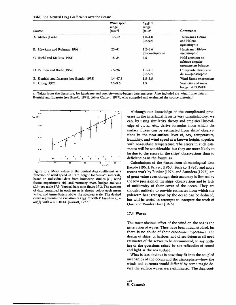
Table 17.3 Neutral Drag Coefficients over the Oceana

Wind speed CDN(10)range range

Source (m s-1) ( x 103) Comments

A. Miller (1964) 17-52 1.0-4.0 Hurricanes Donna(linear) and Helene-

ageostrophicB. Hawkins and Rubsam (1968) 23-41 1.2-3.6 Hurricane Hilda-

(discontinuous) ageostrophicC. Riehl and Malkus (1961) 15-34 2.5 Held constant to

achieve angularmomentum balance

D. Palm6n and Riehl (1957) 5.5-26 1.1-2.1 Composite Hurricane(linear) data-ageostrophic

E. Kunishi and Imasoto (see Kondo, 1975) 14-47.5 1.5-3.5 Wind flume experimentF. Ching (1975) 7.5-9.5 1.5 Vorticity and mass

budget at BOMEX

a. Taken from the literature, for hurricane and vorticity-mass-budget data analyses. Also included are wind flume data ofKunishi and Imasoto (see Kondo, 1975). [After Garratt (1977), who compiled and evaluated the source material.]

C x 10'

0

I I I I I 0

-3'

.

3 6 6 5 2 60 I 5 2 5 3 3 2

l I I 10 20 30 40

V (ms'.

Figure I7.3 Mean values of the neutral drag coefficient as afunction of wind speed at 10-m height for 5-m-s- ' intervals,based on individual data from hurricane studies (O), windflume experiment (), and vorticity mass budget analysis(A)-see table 17.3. Vertical bars as in figure 17.2. The numberof data contained in each mean is shown below each meanvalue, and immediately above the abscissa scale. The dashedcurve represents the variation of CDN(10) with V based on z0 =au2/g with a = 0.0144. (Garratt, 1977.)

Although our knowledge of the complicated proc-esses in the interfacial layer is very unsatisfactory, wecan, by using similarity theory and empirical knowl-edge of z0, ze, etc., derive formulas from which thesurface fluxes can be estimated from ships' observa-tions in the near-surface layer of, say, temperature,humidity, and wind speed at a known height, togetherwith sea-surface temperature. The errors in such esti-mates will be considerable, but they are more likely tobe due to the errors in the ships' observations than todeficiencies in the formulas.

Calculations of the fluxes from climatological data[Jacobs (1951), Privett (1960), Budyko (1956), and morerecent work by Bunker (1976) and Saunders (1977)] areof great value even though their accuracy is limited bythe low precision of the ships' observations and by lackof uniformity of their cover of the ocean. They arethought unlikely to provide estimates from which thepoleward heat transport by the ocean can be deduced,but will be useful in attempts to interpret the work ofOort and Vonder Haar (1976).

17.4 Waves

The most obvious effect of the wind on the sea is thegeneration of waves. They have been much studied, forthere is no doubt of their economic importance: thedesign of ships, of harbors, and of sea defenses all needestimates of the waves to be encountered, to say noth-ing of the questions raised by the reflection of soundand light at the sea surface.

What is less obvious is how they fit into the coupledmechanics of the ocean and the atmosphere-how thewinds and currents would differ if by some magic de-vice the surface waves were eliminated. The drag coef-

490H. Charnock

i:

_

.-

5

ficient for surface friction seems to be largely inde-pendent of the larger waves, as do the exchangecoefficients for heat and water vapor. The transfers ofenergy and momentum from the atmosphere to waveson the ocean have been studied extensively: consider-able progress has been made but there is still no com-plete agreement about the complicated fluid mechanicsinvolved.

The wartime work, well confirmed and extended bySnodgrass and his colleagues (1966), established thebasic fact that swell traveled thousands of kilometers,at the theoretical group velocity, without much atten-uation. This implied that waves did not interactstrongly with each other, or with ocean currents, sothat a Fourier spectral representation was physicallyappropriate as well as mathematically convenient.From it one can derive all the statistical distributionsof the waves for which the model is valid (Longuet-Higgins, 1962). From a practical point of view we mustlearn how to recognize and circumvent the limitationsimposed by nonuniformity of the wind structure, andhow to predict the evolving (directional) wave spec-trum from such meteorological observations as areavailable, or from the output of computer simulations.

17.4.1 The Fetch-Limited CaseAn important but relatively easily realizable case isthat of a steady wind blowing off a straight shore, sothat the duration of the wind is irrelevant and the fetchis well defined. An early contribution to this problemcame from Burling (1959), who measured wave spectraat short fetches on an artificial lake using a newlydeveloped capacitance-wire wave recorder.

In this case one can hope that the energy of thewaves at a given fetch will be proportional to the workdone by the wind on the water. If this is crudely esti-mated as proportional to the shearing stress times adistance measured by the fetch, then

= constant x u,(X/g)" 2 (17.17)

where 2 is the mean square wave amplitude, and X thefetch.

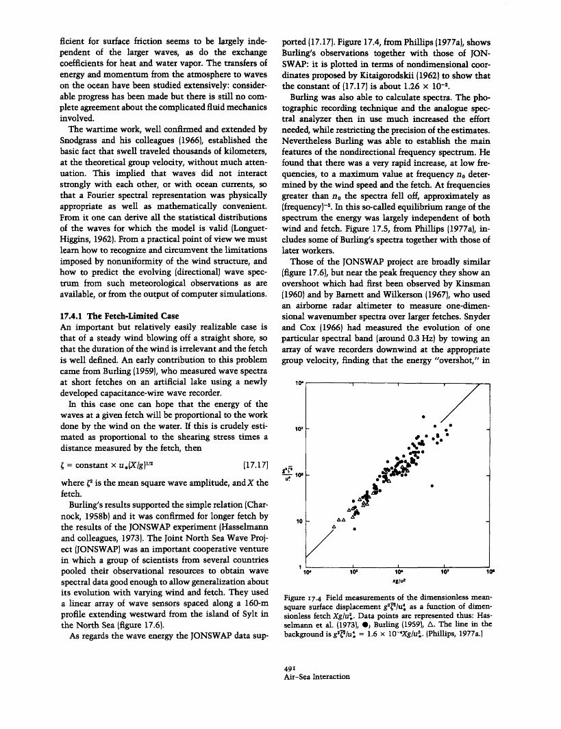
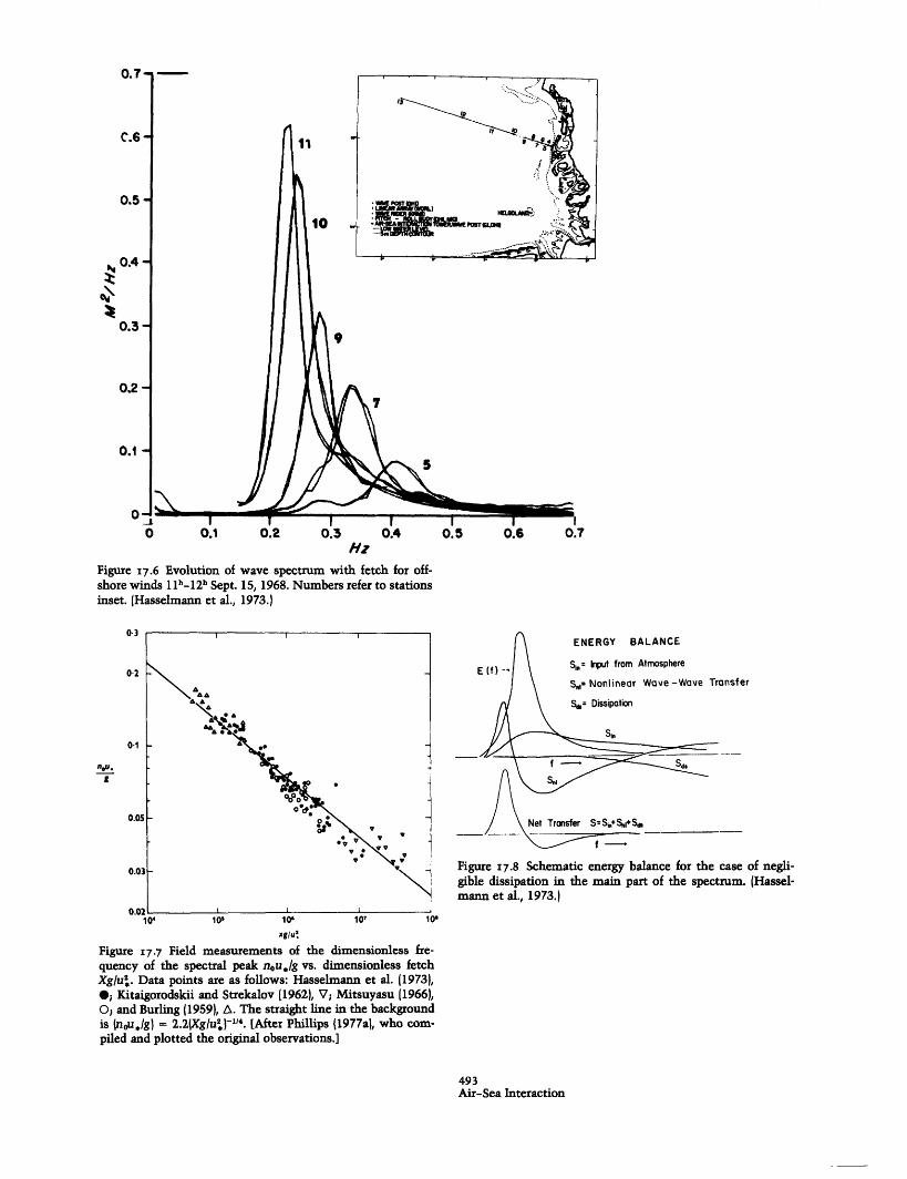
Burling's results supported the simple relation (Char-nock, 1958b) and it was confirmed for longer fetch bythe results of the JONSWAP experiment (Hasselmannand colleagues, 1973). The Joint North Sea Wave Proj-ect (JONSWAP) was an important cooperative venturein which a group of scientists from several countriespooled their observational resources to obtain wavespectral data good enough to allow generalization aboutits evolution with varying wind and fetch. They useda linear array of wave sensors spaced along a 160-mprofile extending westward from the island of Sylt inthe North Sea (figure 17.6).

As regards the wave energy the JONSWAP data sup-

ported (17.17). Figure 17.4, from Phillips (1977a), showsBurling's observations together with those of JON-SWAP: it is plotted in terms of nondimensional coor-dinates proposed by Kitaigorodskii (1962) to show thatthe constant of (17.17) is about 1.26 x 10-2.

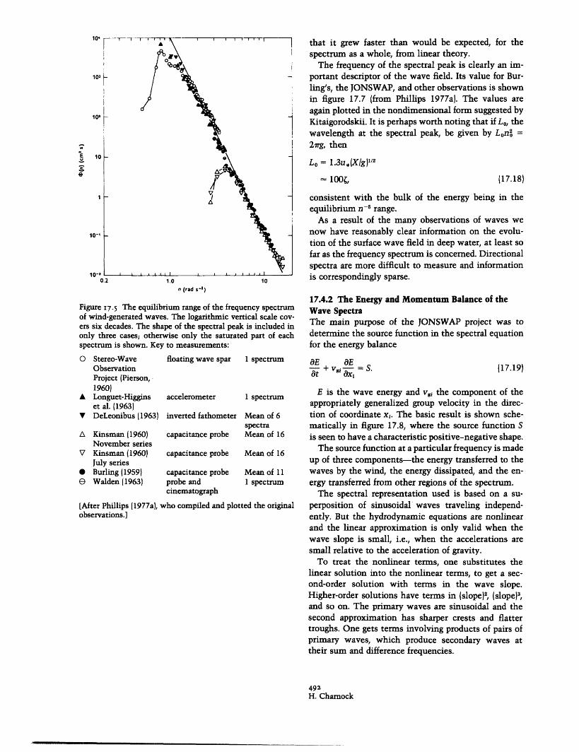
Burling was also able to calculate spectra. The pho-tographic recording technique and the analogue spec-tral analyzer then in use much increased the effortneeded, while restricting the precision of the estimates.Nevertheless Burling was able to establish the mainfeatures of the nondirectional frequency spectrum. Hefound that there was a very rapid increase, at low fre-quencies, to a maximum value at frequency no deter-mined by the wind speed and the fetch. At frequenciesgreater than n, the spectra fell off, approximately as(frequency)-5. In this so-called equilibrium range of thespectrum the energy was largely independent of bothwind and fetch. Figure 17.5, from Phillips (1977a), in-cludes some of Burling's spectra together with those oflater workers.

Those of the JONSWAP project are broadly similar(figure 17.6), but near the peak frequency they show anovershoot which had first been observed by Kinsman(1960) and by Barnett and Wilkerson (1967), who usedan airborne radar altimeter to measure one-dimen-sional wavenumber spectra over larger fetches. Snyderand Cox (1966) had measured the evolution of oneparticular spectral band (around 0.3 Hz) by towing anarray of wave recorders downwind at the appropriategroup velocity, finding that the energy "overshot," in

10'

10o

,,' 10

10

10'

.

* S

0

a

..· O"

A.

10' 10'X/U2

10'

Figure I7.4 Field measurements of the dimensionless mean-square surface displacement g22/u4, as a function of dimen-sionless fetch Xg/u2,. Data points are represented thus: Has-selmann et al. (19731, *; Burling (1959), A. The line in thebackground is g2I/u4 = 1.6 x 10-4 Xg/u2. (Phillips, 1977a.)

49'Air-Sea Interaction

10

I1 I~~~~~~~

J· &

k-

A .

1

that it grew faster than would be expected, for thespectrum as a whole, from linear theory.

The frequency of the spectral peak is clearly an im-portant descriptor of the wave field. Its value for Bur-ling's, the JONSWAP, and other observations is shownin figure 17.7 (from Phillips 1977a). The values areagain plotted in the nondimensional form suggested byKitaigorodskii. It is perhaps worth noting that if L0, thewavelength at the spectral peak, be given by Lon2o =2rg, then

Lo = 1.3u(X/g,)"2

I ] i l * It J I I , ,

0.2 1.0 10n (rad s-')

Figure I7.5 The equilibrium range of the frequency spectrumof wind-generated waves. The logarithmic vertical scale cov-ers six decades. The shape of the spectral peak is included inonly three cases; otherwise only the saturated part of eachspectrum is shown. Key to measurements:

O Stereo-WaveObservationProject (Pierson,1960)

A Longuet-Higginset al. (1963)

V DeLeonibus (1963)

A Kinsman (1960)November series

V Kinsman (1960)July series

* Burling (1959)e Walden (1963)

floating wave spar 1 spectrum

accelerometer

inverted fathometer

capacitance probe

1 spectrum

Mean of 6spectraMean of 16

capacitance probe Mean of 16

capacitance probeprobe andcinematograph

Mean of 111 spectrum

[After Phillips (1977a), who compiled and plotted the originalobservations.]

100C,

consistent with the bulk of the energy being in theequilibrium n-5 range.

As a result of the many observations of waves wenow have reasonably clear information on the evolu-tion of the surface wave field in deep water, at least sofar as the frequency spectrum is concerned. Directionalspectra are more difficult to measure and informationis correspondingly sparse.

17.4.2 The Energy and Momentum Balance of theWave SpectraThe main purpose of the JONSWAP project was todetermine the source function in the spectral equationfor the energy balance

OE OEaE+ vv. - = S. (17.19)at + xi =

E is the wave energy and vsi the component of theappropriately generalized group velocity in the direc-tion of coordinate xi. The basic result is shown sche-matically in figure 17.8, where the source function Sis seen to have a characteristic positive-negative shape.

The source function at a particular frequency is madeup of three components-the energy transferred to thewaves by the wind, the energy dissipated, and the en-ergy transferred from other regions of the spectrum.

The spectral representation used is based on a su-perposition of sinusoidal' waves traveling independ-ently. But the hydrodynamic equations are nonlinearand the linear approximation is only valid when thewave slope is small, i.e., when the accelerations aresmall relative to the acceleration of gravity.

To treat the nonlinear terms, one substitutes thelinear solution into the nonlinear terms, to get a sec-ond-order solution with terms in the wave slope.Higher-order solutions have terms in (slope)2, (slope)3,and so on. The primary waves are sinusoidal and thesecond approximation has sharper crests and flattertroughs. One gets terms involving products of pairs ofprimary waves, which produce secondary waves attheir sum and difference frequencies.

492H. Charnock

10'

10'

102

10E

S9

10-1

10-2

(17.18)

J

N

Figure 7.6 Evolution of wave spectrum with fetch for off-shore winds 1 h-1 2h Sept. 15, 1968. Numbers refer to stationsinset. (Hasselmann et al., 1973.)

onsfer

Figure I7.8 Schematic energy balance for the case of negli-gible dissipation in the main part of the spectrum. (Hassel-mann et al., 1973.)

xglu

Figure I7.7 Field measurements of the dimensionless fre-quency of the spectral peak nou./g vs. dimensionless fetchXg/u.. Data points are as follows: Hasselmann et al. (1973),0; Kitaigorodskii and Strekalov (1962), V; Mitsuyasu (1966),0; and Burling (1959), A. The straight line in the backgroundis (n0u./g) = 2.2(Xg/u 1)- 1 4. [After Phillips (1977a), who com-piled and plotted the original observations.]

493Air-Sea Interaction

no.u/-OU

An~

The solution stays bounded provided there is nocombination of

k3 = k k and n3 = n + n2

such that

gk3 = n.

O. M. Phillips (1963) showed that no such combi-nation occurs in surface gravity waves. But for tertiarywaves he found that for

k4 = k, k2 k3,(17.20)

n4 = n n2 + n

there exist combinations for which gk4 = n4, so thereis a resonance, with energy being transferred from threeprimary waves to a new wave whose energy growslinearly with time. The interactions are weak, so itgrows slowly, its time scale being of order (slope)4

times a typical wave period. Such nonlinear interac-tions have been observed in careful laboratory experi-ments and shown to be consistent with the slow at-tenuation of ocean swell.

Hasselmann (1966) has exploited the analogy withcollisions in high-energy physics, and he uses Feynmandiagrams to represent nonlinear interactions, withwavenumber corresponding to momentum and fre-quency to energy. He has also given a complicatedequation by which the nonlinear transfers can be cal-culated. Using an interaction equation derived by Lon-guet-Higgins (1976), Fox (1976, 1978) has given a sim-pler method applicable when the spectrum is narrow.Broader spectra have been studied by Webb (1978).

For the JONSWAP case Snt, the contribution of non-linear transfer is shown on figure 17.8. It has the samepositive-negative shape as S and provides a reasonablequalitative explanation of the way in which the spec-tral peak goes to lower frequencies as the nondimen-sional fetch increases.

The contribution of Sn1, due to nonlinear weak in-teractions, is to redistribute wave energy within thespectrum. It is the best known of the terms that makeup S:

S = Sin + Snl + SdS (17.21)

where Sin represents the energy input from the atmos-phere and Sds the dissipation. Assuming the dissipationto be small in the energetic low-frequency band of thespectrum, the JONSWAP results indicate a schematicenergy balance as in figure 17.8. Then the energy inputhas a distribution like that of the spectrum itself, as ifthe wave generation depends linearly on the spectrum,and the dissipation occurs mainly at high frequencies.

Attempts to calculate Sin theoretically have so farbeen unsuccessful. It involves the calculation of the

covanances between fluctuations in the surface stress(both normal and tangential) and in the surface veloc-ity. Phillips (1957) showed that turbulent pressure fluc-tuations in the natural wind would amplify waves trav-eling at the right convection velocity by a resonancemechanism. Like an earlier theory of Eckart (1953), thetheory was qualitatively correct but the amplitude ofatmospheric pressure fluctuations (rms pressure fluc-tuation To0) was too small to produce waves of theamplitude observed. Miles (1957, 1959) calculated fluc-tuations induced by the mean wind blowing over thewavy surface: since the pressure fluctuations dependon the wave amplitude, the latter grows exponentially,but again the predicted growth rate was much less thanthat observed. Miles had been obliged to neglect theatmospheric turbulence in the interfacial layer, how-ever, and nobody has yet succeeded in satisfactorilyincorporating it. The problem was carefully discussedby Davis (1972), who used several different closureapproximations, which gave variable results. He alsofound that the rate of energy transfer to the waves iscritically dependent on the profile of mean flow veryclose to the interface. Gent and Taylor (1976), whohave done numerical simulations of airflow overwaves, avoided the problem by assuming that the sur-face has an assigned roughness, either constant or dis-tributed along a long wave. Their solutions are moreencouraging but the problem of calculating energy andmomentum transfer in the interfacial layer is by nomeans solved.

Detailed observation of energy and momentumtransfer in the interfacial layer also presents great dif-ficulty. Since the drag coefficient of the sea surface isgreater, but not very much greater, than that of anaerodynamically smooth surface, one might expectsome direct viscous transfer. In this case the tangentialstress must be supported, just below the interface, bya thin layer with strong shear. Equally, since the seasurface becomes increasingly rough, relative to an aero-dynamically smooth surface, as the wind speed in-creases, there must be a good deal of momentum trans-port to irrotational or quasi-irrotational waves bypressure fluctuations. This was the basis of Jeffreys's(1925) theory. Valiant attempts have been made tomeasure pressure fluctuations relative to the wave pro-file by Dobson (1971), Elliott (1972), and Snyder (1974).

Such observations are extremely difficult. The staticpressure fluctuations 0(T0 ) are small, very small rela-tive to the dynamic pressures in the airflow. To com-pute the energy and momentum transfer to the waves,the pressure is needed at the (moving) surface: thisneeds an extrapolation from a recorder as near the sur-face as possible, or a surface-following device, whichintroduces other problems. It is hardly surprising thatthe early results were not entirely consistent: roughlyspeaking Dobson's values gave the biggest growth

494H. Chamock

rates, Elliott's were smaller (roughly ) and Snyder'seven less.

These three authors have recently collaborated withLong in a field program in the Bight of Abaco in theBahamas (Snyder, Dobson, Elliott, and Long, 1980). Pre-liminary results indicate that momentum transfer tothe wave extends from the peak frequency to at leasttwice the peak frequency with little noticeable falloff.Observations at higher frequency will be necessary toallow an estimate of the total momentum transfer, butit seems clear that for the JONSWAP spectrum a sig-nificant fraction of the momentum first goes intowaves; about 10% at long fetch (gX/U2o = 105), rising toabout 100% at shorter fetch (gXI/U20 = 102). There re-mains a need for critical observations at short fetch,but the high-frequency response that will be neededwill be hard to achieve.

The dynamics of a near-surface viscous shear layerare also relevant: Banner and Phillips (1974) haveshown that the speed of such a layer will be increasednear the crest of a longer wave, so leading shorter wavesto break. Such breaking may be made visible by dim-ples or pockmarks on the surface, particularly in theearly development of a wave field. Banner and Melville(1976) have demonstrated that wave breaking, even ona small scale, is accompanied by separation of the air-flow from the surface. This has strong implicationsboth for momentum transfer and for the exchange ofheat or water vapor. That the drag and analogous coef-ficients are small may prove to be due to the sporadicnature of the breaking process. The problem deservesfurther investigation since breaking waves seem to pro-vide a limit between the spectrum of the longer Gaus-sian waves and the shorter nonlinear ripples: breakingwaves on the open sea have been much neglected(Charnock, 1958a).

Another important phenomenon associated withbreaking waves, with which one hopes more progresswill be made in the next 20 years than in the last, isdissipation. It now seems more likely that breakingwaves are more important than viscosity in dissipation,and Longuet-Higgins (1969a) has given an interestingcalculation that implies that the proportion of waveenergy lost per mean cycle is about 10-4.

Measurements of mean and fluctuating velocities inwaves are technically difficult, but there is growingevidence that the orbital velocities of the larger wavesare inactive, in the sense that they provide variancebut are so uncorrelated as to be inactive in the transferof momentum. Jones and Kenney (1977) have arguedthat the near-surface layer in the water has many ofthe characteristics of the surface layer in the air, withscaling on u, and z0. Observations by Donelan (1978)show that as well as the wave orbital velocities thereare fluctuations at lower frequency (possibly due tothe shear in the mean profile) and at higher frequency

(possibly due to whitecapping). The momentum fluxwas entirely due to the low-frequency fluctuations. Hisgeneral picture of the effects of wave breaking is thatthe wind stress produces a strongly sheared currentnear the surface, so that when a wave breaks the down-ward pulse of fluid produces a downward momentumtransfer. Though each pulse of momentum is short, theintermittent nature of the phenomenon is reflected inthe momentum flux at lower frequencies. The effect ofwhitecapping on the spectrum has been considered the-oretically by Hasselmann (1974) as a strong interactionthat is weak in the mean: because it is sporadic andlocal in physical space the energy loss is spread overmuch of the spectrum.

17.4.3 Langmuir CirculationsAnother near-surface phenomenon that may be impor-tant in momentum transfer is the Langmuir cell. Lang-muir cells are alternate left-handed and right-handedvortices in the vertical plane (horizontal rolls), alignedalong the wind with surface velocities strongest in theconvergence zones. It is easy to see that the strongerhorizontal velocity there could combine with the sink-ing motion under the convergence zone to give meanstresses of the same order as the wind stress at thesurface.

There have been many observations since Lang-muir's (1938) first description, all supporting the cel-lular structure he found. Row spacings, often markedby streaks on the surface, are variable, typically 10 min lakes and 100 m over the ocean: the surface currentmoves at about 10 cms - 1 faster in the streak thanoutside it. The vertical structure is less well known.An account of the observations is given by Pollard(1977); he also gives an account of theoretical attemptsto explain these cells, from which it seems clear thatcomplicated interactions in the surface wave field areinvolved. Faller (see chapter 16) has shown in labora-tory observations that both wind and waves are nec-essary for the generation of Langmuir cells: it isthought that the vorticity of the shear flow producedby the wind stress is transformed by nonlinear inter-action with crossing wave trains into the vorticity ofthe helices. The details are complicated but it seemslikely that the Langmuir cells may represent a mech-anism by which wave energy is converted to organizedconvection and to turbulence, which in turn may actto deepen the mixed layer.

17.5 The Atmospheric Boundary Layer

From a practical point of view the mean fluxes at thesea surface can now be calculated to acceptable accu-racy from observations in the surface layer. The relatedcharacteristics of the surface wave field are also rea-

495Air-Sea Interaction

sonably well known and it can be assumed, with some-what less confidence, that the momentum transferredfrom the atmosphere to the sea surface is then trans-ferred to the ocean at the same place and time.

In all these cases our knowledge is empirical andthere is a need for more understanding, leading to the-oretical descriptions of the physical processes involved.But from an engineering viewpoint what was oncethought of as the central problem of air-sea interactionhas been reduced to some sort of order.

Problems change, however, and those of air-sea in-teraction are now of much greater scope. The recentlyrenewed interest in climate and climatic change hasled to a wider appreciation of the importance of theinteraction between the atmosphere, the ocean, andcharacteristics of solid surfaces such as ice. Becausealmost all the energy for the motion comes from thesun it is conceptually attractive to regard the basiccirculation of the atmosphere and ocean as the freeconvective response of the coupled system to solarheating. Air-sea interaction can now be taken to in-clude all the problems of meteorology and oceanogra-phy.

Nevertheless the different physical properties of airand water, especially their relative opacities to electro-magnetic radiation, lead to considerable decoupling:the mismatch is such that it is usually more rewardingto treat them separately, isolating topics like the effectof wind on the sea, or the effect of evaporation on theatmosphere. The darkness of the ocean has also madeobservations difficult, so less is known of its structurethan that of the relatively transparent atmosphere.

No one disputes that the fluxes of heat, water vapor,and momentum that enter the atmosphere through itslower boundary layer are of crucial importance to thedevelopment of atmospheric flow patterns and weatheron time scales ranging from minutes to months. Thereis no reason to doubt that they are equally importantfor longer-period climatic changes, but we know littleof the degree of accuracy and detail in which they mustbe described for specific purposes, in particular for fore-casting using computer models of the atmosphere, theocean, or the coupled system.

Some suggestion that rather precise knowledge ofthe exchange processes will be needed comes from therelations that have been found (Namias, 1969;Bjerknes, 1969; Ratcliffe and Murray, 1970) betweensea-surface temperature anomalies and subsequentweather patterns, though a direct causal connectionhas not been unambiguously demonstrated. To achievesuch precision an understanding of the physical proc-esses involved seems essential: attempts to use param-eters without physical understanding may yield rapidprogress in the early stages but seem likely to be in-adequate in the long run.

At any given time atmospheric and oceanic motionson scales greater than 100 km or so can be treated asessentially inviscid and adiabatic, but there are local-ized regions where condensation processes, or thetransport of heat, water, salt, or momentum by small-scale turbulence are important, even dominant. Ex-amples of such regions are towering clouds, or groupsof clouds, fronts, and the turbulent boundary layersnear the earth's surface. For the present purpose it hasseemed sensible and convenient to restrict the scopeof air-sea interaction to studies of the mechanics andstructure of the near-surface boundary layers of theatmosphere and the ocean.

For many years, as has been indicated, the subjectwas more restricted, essentially to the lowest 10 to100 m of the atmosphere above the sea. This cameabout mainly because the routine observations avail-able were those from ships. There were a few upper-airobservations from weather ships, but their purpose wasto map meteorological fields in the troposphere andlower stratosphere: exchanges with the ocean were notallowed for in routine forecasting.

Routine observations of the whole atmosphericboundary layer over the sea are still virtually non-existent, the number of weather ships having decreasedin recent years. What has developed rapidly is the nu-merical simulation of atmospheric processes, now usedroutinely as a basis for weather forecasting: when theseare used to forecast for more than a day or so it beginsto be necessary to include boundary-layer effects. Somemodels use many layers in an attempt to resolve thevertical structure of the boundary layer, ultimately re-lating fluxes to conditions in the surface layer, but theneed to simulate small-scale turbulence in the bound-ary layer makes such a system prohibitively expensivein computer time unless the equations are drasticallysimplified. It seems more realistic to admit that theboundary layer has a different physics from most of theatmosphere above it and to seek to treat it as a whole.Then the height of the top of the atmospheric boundarylayer is calculated explicitly and becomes the effectivelower boundary of the largely frictionless atmosphereabove. Such a method was adumbrated by Charnockand Ellison (1967) and has been developed by Deardorff(1972) and implemented by Arakawa (1975). The struc-ture of the atmospheric boundary layer is now beingincreasingly studied, but it is much more complicatedthan the surface layer. It is not well mapped, nor arethe physical processes that maintain it well under-stood.

The top of the atmospheric boundary layer is usuallymost obvious from inspection of the density variationwith height, particularly over land in summer. Then aweakly stable condition is established during the nightthat is transformed after dawn by solar heating to aconvective boundary layer at the surface. This is suf-

496H. Chamock

�_

ficiently well mixed to have effectively constant po-tential temperature, and it deepens as it warms in ac-cordance with the classical ideas of Gold 1933). It iseasy to check that there is reasonable quantitativeagreement between the available solar energy and therate of warming of the boundary layer. That the levelof turbulence inside such a convective boundary layeris much greater than in the free air above is obvious toanyone who has done much flying, but of course it canbe confirmed instrumentally. It is also common to findthat smoke or other pollutants are fairly uniformlymixed in the boundary layer but that the air above isrelatively clean.

Over land there is a pronounced diurnal variabilityand a great range of boundary layer depths: over thesea there is little diurnal change but much variabilityfrom day to day.

17.5.1 Unstable Boundary LayersGiven the original records it is possible to obtain a fairrepresentation of unstable boundary layers from rou-tine radiosonde ascents. Figure 17.9 shows a character-istic diagram obtained from the ascent at OceanWeather Station (OWS) India (59°N, 19°W) at 2330Z on10 March 1966. The variables plotted are the potentialtemperature 0 and the specific humidity q, both ofwhich are conserved in adiabatic motion and obey thesimple law of mixtures. The q-0 diagram was used byTaylor (1917) as a tool for studying the atmosphericboundary layer and is sometimes called the Taylor dia-gram. The analogous S-O diagram is widely used inoceanography, but the great convenience of the Taylordiagram has not been widely recognized in spite of acomprehensive review by Montgomery (1950).

For the ascent plotted it will be seen that the pointscorresponding to heights up to 908 mb are clusteredtogether, indicating a high degree of mixing: higher up,the density gradient is definitely stable. The point rep-resenting air in contact with the sea is at a potentialtemperature 5°C higher than that typical of the mixedlayer. The point corresponding to the observations atdeck level theoretically would be expected to be on theline joining the mixed layer to the sea surface: that thesurface values are lower is difficult to explain.

Figure 17.10 is a similar diagram from an ascent atGan (0°41'S, 73°09'E). Some workers, influenced byEkman's theory of the variation of wind with height,have predicted very deep boundary layers near theequator: that such a view is not borne out by obser-vation goes some way toward demonstrating that thethickness of the boundary layer is determined more bythe density structure.

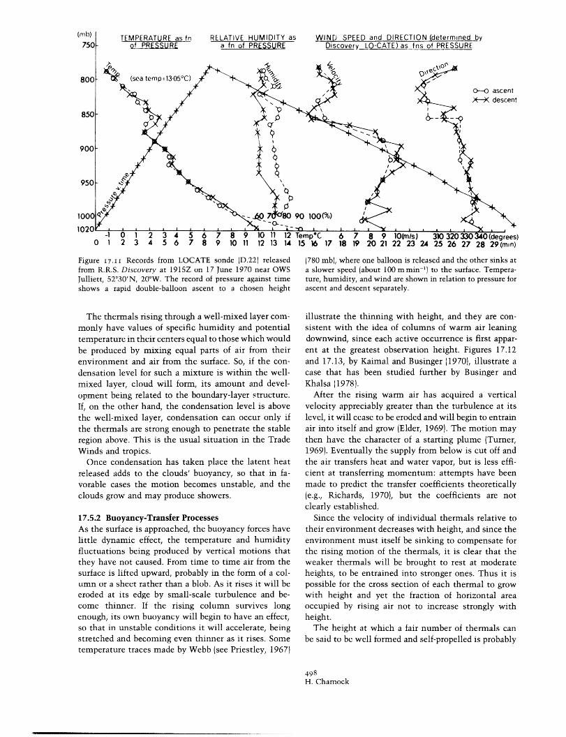
Figure 17.11 gives the results of a special slowlyrising ascent at OWS Julliet (52°30'N, 20°W). More

6

1 2 3 4 5 6 7103q

Figure I7.9 Characteristic diagram, OWS India (59°N, 19°W),on 10 March 1966.

30

292

28

103q

Figure I7.IO Characteristic diagram, Gan (0°41'S, 73°0 9'E),on 25 July 1967.

detail is given, but the structure is basically similar tothat in figures 17.9 and 17.10. The wind profile at thesame time shows that the wind varies slowly withheight in the mixed layer, but that there is considerableshear at the boundary-layer top.

There remains a need for long-term studies of thecharacter of the boundary layer over the sea so thattheir climatology can be established. A pilot study ofthe ascents at OWS India (59°N, 19°W) for March 1966showed that more than half had reasonably well-de-fined unstable boundary layers. The boundary layerdepth ranged from 200 to 2000 m, being at most weaklycorrelated with the vertical potential temperature dif-ference between the sea surface and the mixed layer,which ranged from 0 to 9°C.

Even in convective conditions a well-mixed statewith potential temperature independent of height isnot always found, and it may be difficult to determinethe depth of the boundary layer from the sounding.Also, when a well-mixed layer does exist it may betopped by a layer of relatively weak stability into whichthe stronger convective motions from below can pen-etrate a considerable distance.

497Air-Sea Interaction

I l

I I 1006 I I

I

I

WIND SPEED and DIRECTION (determined byDiscovery LO-CATE) as fns of PRESSURE

9 10 11 12 13 14 15 16 17 18 19 20 21 22 23 24 25 26 27 28 29(mn)

Figure I7.II Records from LOCATE sonde (D.22) releasedfrom R.R.S. Discovery at 1915Z on 17 June 1970 near OWSJulliett, 52°30'N, 20°W. The record of pressure against timeshows a rapid double-balloon ascent to a chosen height

The thermals rising through a well-mixed layer com-monly have values of specific humidity and potentialtemperature in their centers equal to those which wouldbe produced by mixing equal parts of air from theirenvironment and air from the surface. So, if the con-densation level for such a mixture is within the well-mixed layer, cloud will form, its amount and devel-opment being related to the boundary-layer structure.If, on the other hand, the condensation level is abovethe well-mixed layer, condensation can occur only ifthe thermals are strong enough to penetrate the stableregion above. This is the usual situation in the TradeWinds and tropics.

Once condensation has taken place the latent heatreleased adds to the clouds' buoyancy, so that in fa-vorable cases the motion becomes unstable, and theclouds grow and may produce showers.

17.5.2 Buoyancy-Transfer ProcessesAs the surface is approached, the buoyancy forces havelittle dynamic effect, the temperature and humidityfluctuations being produced by vertical motions thatthey have not caused. From time to time air from thesurface is lifted upward, probably in the form of a col-umn or a sheet rather than a blob. As it rises it will beeroded at its edge by small-scale turbulence and be-come thinner. If the rising column survives longenough, its own buoyancy will begin to have an effect,so that in unstable conditions it will accelerate, beingstretched and becoming even thinner as it rises. Sometemperature traces made by Webb (see Priestley, 1967)

(780 mb), where one balloon is released and the other sinks ata slower speed (about 100 m min-') to the surface. Tempera-ture, humidity, and wind are shown in relation to pressure forascent and descent separately.

illustrate the thinning with height, and they are con-sistent with the idea of columns of warm air leaningdownwind, since each active occurrence is first appar-ent at the greatest observation height. Figures 17.12and 17.13, by Kaimal and Businger (1970), illustrate acase that has been studied further by Businger andKhalsa (1978).

After the rising warm air has acquired a verticalvelocity appreciably greater than the turbulence at itslevel, it will cease to be eroded and will begin to entrainair into itself and grow (Elder, 1969). The motion maythen have the character of a starting plume (Turner,1969). Eventually the supply from below is cut off andthe air transfers heat and water vapor, but is less effi-cient at transferring momentum: attempts have beenmade to predict the transfer coefficients theoretically(e.g., Richards, 1970), but the coefficients are notclearly established.

Since the velocity of individual thermals relative totheir environment decreases with height, and since theenvironment must itself be sinking to compensate forthe rising motion of the thermals, it is clear that theweaker thermals will be brought to rest at moderateheights, to be entrained into stronger ones. Thus it ispossible for the cross section of each thermal to growwith height and yet the fraction of horizontal areaoccupied by rising air not to increase strongly withheight.

The height at which a fair number of thermals canbe said to be well formed and self-propelled is probably

498H. Chamock

0 1 2 3 4 5 6 7 8

_ ___II�_I

)

30 35 40 45 50 55 0 5 10 15

TIME (s) '

64

-2

64

-2

-2

E

4I2'0

2-4

42

I C-2-4

I I I I I I I I I

_ (22.6m) I I

I - I

I I

_ u (5.66m) ! -I

I11 I I I II I I

I I I I I I I I I I

30 35 40 45 50 50 0 5 10 15

t/ME $(s

Figure I7.IZ Traces of u, v, w and T (temperature) duringpassage of a convective plume. (Kaimal and Businger, 1970.)

UA z5.Om s -

uB= 3.5ms -1

WA= 2.0 m s-I

Wl= 1.0 m s-

wA

FRONT

Figure I7.I3 Two-dimensional model of a convective plume.(Kaimal and Businger, 1970.)

499Air-Sea Interaction

2IDIa

21012

i

t"I:.

32

0* 1.2

2

0-21.2

l I I I I I I I I I

w(22.6m) I

I I

- w (5.66 m)

- I I _1. 1 1 1 1 1 1 1a

I

I I I I I I I I I i

T'(22.6m)

I I

_ -0.13'C I

T'( 5.66m) I_ I I I -

- -044C 1305(CDT) : -I Is I T I XI I

I I I I I I I I I I

- v (22.6m)

I I

v (5.66 m

I I --

1305 (CDT)

I I I I I I I I I

· · · 1 1 ·

! , */

· ·. ·..·:···:·: ··:i·:

:·· · ·"··

·:···:�. .:.·:·:·:·:

·:::::';�': :�

· ·�::

above the surface layer, where the temperature gradientand the wind shear are determined by the similarityrules. In particular the wind shear may be governed bythe variation of the geostrophic wind with height.There is some evidence that when this is large there isa tendency for motions of scale comparable with thedepth of the boundary layer to become organized intolarge longitudinal roll vortices. Given an appropriatecondensation level, one would expect such motions tobe visible in pictures of clouds taken from high-flyingaircraft or from satellites, and many such images havebeen interpreted in this way; see, for instance, Ageeand Dowell (1974) and Kuettner (1971). The patternsalso depend on the general vertical motion due to con-vergence or divergence on the mesoscale or the syn-optic scale.

The importance of clouds in the transport process isclear from studies that evaluate the heat or water budg-ets of the subcloud layer and the cloud layer separately.Riehl, Yeh, Malkus, and La Seur (1951) in a classicalstudy found that as much as four-fifths of the waterevaporated from the sea entered the cloud layer. Thisis a high value, to explain which it has been suggestedthat the transport is concentrated into localized areaswhere there are cloud groups or clusters. But the samesort of thing happens in polar outbreaks, with well-spaced clouds, so it seems likely that cumulonimbusclouds must suck up a large volume of the subcloudlayer between them. Browning and Ludlam (1962) sug-gest a cumulonimbus model in which strong down-drafts partially compensate for the upflow, but in gen-eral there will be shrinking and subsidence in thesubcloud layer in the space between clouds. The roleof the heat and water-vapor fluxes from the surface isthus in the first instance to maintain the depth of thewell-mixed layer rather than to feed directly into thelayer clouds.

17.5.3 Stable Boundary LayersStable boundary layers, on the other hand, are difficultto investigate using routine observations. They areoften relatively shallow, with small temperature dif-ferences, and since the transports of heat and watervapor are small, they have attracted little attention.There are few satisfactory sets of observations, but theycan be interpreted as showing that heat is transferredto the surface until an almost linear gradient of poten-tial density is formed from the surface to height h,where the difference in potential temperature AO isgiven roughly by

g - h/Uo = 0.5. (17.22)

Hanna (1969) attributes (17.22) to Laikhtman (1961),and gives an example using O'Neill's data (Lettau andDavidson, 1957) that supports it.

Over the sea, figure 17.14, by Craig (1946), showsascents made at three different fetches in warm con-tinental air flowing out over colder sea. At the largestfetch

g A h/U2 - 0.4.

One of the classical ascents made by Taylor (1914)on the S.S. Scotia provides another example (the othersare not suitable because of fog), which is shown infigure 17.15. Here

g- h/U2 - 0.35.

17.5.4 Wind in the Boundary LayerTurbulent friction in the boundary layer causes thewind to deviate from its frictionless value, and earliersections have shown how it increases rapidly, roughlyas the logarithm of the height in the lowest few meters.From a height of 30 m or so there is usually relativelylittle change until the top of the boundary layer isreached. Sometimes there is a significant and rapidchange with height at the top of the boundary layeruntil the frictionless value is attained.

The wind changes not only in speed but in directionalso. Such changes were predicted by Ekman for theocean and soon applied to the atmosphere by Akerblomand (some years later, independently) by Taylor. Be-cause they took a constant value for the eddy viscosityKM they got the well-known Ekman spiral for the ho-dograph. Perhaps more important is their deductionthat in stationary conditions, when the boundary layerhas a finite depth H, with zero stress above,

H

u2 = fV- Vg)dz,

(17.23)

o =ffAU - Ug)dz,

where Ug, Vg are the components of the geostrophicwind.

This result is independent of the mechanism oftransfer: it relates the surface stress to the cross-isobartransfer, and provides a basis for calculating the fric-tional convergence and so the mean vertical velocityat the top of the boundary layer. This, in turn, has aneffect on the motion of the whole atmosphere. Unfor-tunately, conditions are rarely so simple as to allow adirect application of (17.23).

Much subsequent work has sought to use more com-plicated expressions for KM(z), to try to predict Ku(z)theoretically, or to deduce it from observations. It isnow known that the variation of the pressure gradientwith height often has a large influence on the anglebetween the geostrophic and the surface wind; and that

500H. Chamock

_�__

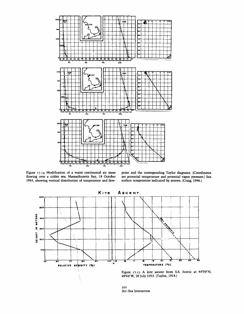
Figure I7.I4 Modification of a warm continental air massflowing over a colder sea, Massachusetts Bay, 18 October1944, showing vertical distribution of temperature and dew-

point and the corresponding Taylor diagrams. (Coordinatesare potential temperature and potential vapor pressure.) Seasurface temperature indicated by arrows. (Craig, 1946.)

.A430

O'rl448'W, 29 July 1913. (Taylor, 1 914.) t JV.u 49°48'W, 29 July 1913. {Taylor, 1914.1

501Air-Sea Interaction

K ITE A sc E NT.

co0hi

I-W2_

Icozom

variations of KM in time, or in the downstream direc-tion, can lead to oscillations in which the flow in themiddle of the boundary layer can increase considerablyabove its geostrophic value, giving rise to the so-calledlow-level jet.

Since it is known that near the surface KM = KUZ

and that in neutral conditions this is a fair approxi-mation up to 100 m or so, it is obviously worth ex-amining the implications of assuming it true at allheights (Ellison, 1956). The results agree reasonablywell with measured wind profiles, but this showsmerely that they are insensitive to KM above the surfacelayer. This does not vitiate, however, Ellison's dem-onstration that the thermal wind has a large effect.

Nevertheless in the (very rare) case when the strati-fication is so nearly neutral that it can be neglected,Kazanskii and Monin (1960, 1961) dealt with the prob-lem in a convincing way. In these papers they intro-duced a similarity argument for the entire boundarylayer that has since been discussed by Csanady (1967),Gill (1968), Blackadar and Tennekes (1968), Zilitink-evich (1969, 1970), and others. This is based on a com-bination of the surface-layer arguments, leading to thelogarithmic wind profile together with a velocity defectlaw that asserts that

U-= f(zIH) + a velocity of translation.

For the atmospheric boundary layer, the boundarylayer thickness H is taken as u,/f, where f is the Cor-iolis parameter. The result is, for neutral conditions

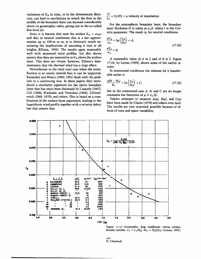
+U,A,(17.24)

KV= B.U,

A reasonable value of A is 2 and of B is 5. Figure17.16, by Lettau (1959), shows some of the earlier re-sults.

In nonneutral conditions the relation for a transfer-able scalar is

(17.25)K( - 0) U= In(fU)+ C,0, I OO

but in the nonneutral case A, B, and C are no longerconstants but functions of ,u-u u*IfL.

Valiant attempts to measure A(/t), B(t), and C(.)have been made by Clarke (1970) and others over land.The results are very scattered, possibly because of ef-fects of time and space variability.

4.5 5.0 5.5 6.0 6.5 7.0 7.5 .o 8.5 9.0 9.5

LOG o,

Figure 7.i6 Geostrophic drag coefficient versus surfaceRossby number. Ca = u, /[V,I, Ro0 = IVg/(fzo). (Lettau, 1959.)

502H. Chamock

0.050

0.045

0.040

0.035

Co

0.030

0.025

0.020

0.015

There seems to be no way to avoid the need for anevolving model of the boundary layer in which theheight of the top will be predicted. This will dependon advection, on the (frictional and frictionless) con-vergence, and on the entrainment of the air above. Inthis sense the early single-point measurements (Shep-pard, Charnock, and Francis, 1952; Charnock, Francis,and Sheppard, 1956) and others well described by Roll(1965) are of limited value. More recent studies havebeen large acronymic projects like ATEX (Augstein,Schmidt, and Ostapoff, 1974), BOMEX (Holland andRasmusson, 1973), GATE, AMTEX (Ninomiya, 1974)and JASIN (Taylor, 1979), from which no simple resulthas yet been distilled.

A climatological study has been made by Findlater,Harrower, Howkins, and Wright (1966): this and relatedwork is reported by Sheppard (1970), from whom figure17.17 is taken. The geostrophic drag coefficient impliedby (17.24) must also be consistent with the require-ments of the angular-momentum balance of the earth,and La Valle and Di Girolamo (1975) have thus founda mean value (= u2/lVgl2) of 0.41 x 10-3.

Even in cloud-free conditions the dynamics of theatmospheric boundary layer is complicated: it is notyet clear which are the most important transfer proc-esses or how they can be dealt with.

(a) OWS I

17.5.5 The Upper Boundary Layer of the OceanThe near-surface boundary layer of the ocean has muchin common with that of the atmosphere. It is mostobvious from the vertical density structure: more orless well-mixed layers are to be found near the surfaceover most of the ocean most of the time. As in theatmosphere the velocity structure is not well known(it is difficult to measure currents in the presence ofwaves), but the simple Ekman-type distributions arerarely found.

Like the atmospheric boundary layer, the oceanicboundary layer is maintained by a combination of ad-vection, surface fluxes, and entrainment at the lowersurface. Because vertical gradients are much biggerthan those in the horizontal, the advection can oftenbe neglected: the basis of the resulting one-dimensionalmodels is well described by Niiler and Kraus (1977),and details of the complicated mixing processes aregiven by Turner (chapter 8).

(b) OWS J

.122<34

52

345

15 25 35 45 ,50

30

20

10

0

5

1 X

15 25 35 45 >50

15 25 35 45 ,50

~1

12

15 25 35 45 50

900-mb wind-speed class (knots)

Figure I7.17 The variation of the ratio between the windspeed at the surface (Vo) and at 900 mb (Vo}) and of the anglebetween them (a) in relation to Vg,0 mb and the mean lapserate from surface to 900 mb at OWS India and Julliett. Thepoints refer to classes in wind speed (kt): 10-19, 20-29, 30-39, 40-49, >50, and in lapse rate (°F/1000 ft = 1.69°C/km):>5.5 (1), 5.4 to 4.0 (2), 3.9 to 2.5 (3), 2.4 to 1.0 (4), 0.9 to-0.5 (5). Smaller lapse rates and lower wind speeds excluded.Lapse class shown against end of curves. Number of obser-vations in each class when less than 100 shown in parenthe-ses. (Due to Findlater et al., 1966.)

503Air-Sea Interaction

I.uI.u

09

VoV900

08

0-7

0'6

n'.c

30

20

a 10

0

Vu3 ' ' ' '~~~~~~~