T-FLEX Dynamics - SoliCAD.comsolicad.com/media/download/tflex/manual/tflex_dynamics_um.pdf · T-FLEX Dynamics User Manual General Information The dynamic analysis module is integrated

T-FLEX DYNAMICS USER MANUAL

«Top Systems» Moscow, 2016

© Copyright 2016 Top Systems This Software and Related Documentation are proprietary to Top Systems. Any copying of this documentation, except as permitted in the applicable license agreement, is expressly prohibited. The information contained in this document is subject to change without notice and should not be construed as a commitment by Top Systems who assume no responsibility for any errors or omissions that may appear in this documentation. Trademarks: T-FLEX Parametric CAD, T-FLEX Parametric Pro, T-FLEX CAD, T-FLEX CAD 3D, T-FLEX Analysis, T-FLEX Dynamics are trademarks of Top Systems. Parasolid is a trademark of Siemens PLM Software. All other trademarks are the property of their respective owners.

Table of Contents

TABLE OF CONTENTS

General Information ...................................................................................................................................... 4 The Structure of a Dynamic Calculation Study ....................................................................................................... 5

Rules of Performing Dynamic Calculations ................................................................................................. 8 Study Management Utilities .................................................................................................................................... 8 Creating Study ......................................................................................................................................................... 9 Study Parameters ................................................................................................................................................... 11 Joints ..................................................................................................................................................................... 13 Creating Loads ...................................................................................................................................................... 14 Creating Sensors .................................................................................................................................................... 20 Creating Results. Result Types ............................................................................................................................. 21 Running Calculations ............................................................................................................................................ 22

Limitations of the Express Dynamics Analysis Module ............................................................................. 25

3

T-FLEX Dynamics User Manual

General Information The dynamic analysis module is integrated with T-FLEX CAD 3D. The module uses proprietary algorithms developed by Top Systems engineers and serves to investigate the dynamical behavior of various three-dimensional mechanical systems. The dynamic express analysis module is readily available as T-FLEX CAD 3D built-in. This is a free noncommercial version intended primarily for getting acquainted with the main module. The Express Dynamics module has certain limitations on load types and the display of dynamic analysis results. This chapter describes the capabilities of the program and the rules of working with the main module, as well as provides the list of limitations and the differences in the Express Dynamics module operation. The dynamical analysis system is capable of solving the following studies:

• Analysis of the motion trajectory, velocity and acceleration of any point of a component in a mechanical system under applied forces;

• Analysis of performance times of a mechanical system (the time to the target point, the time for vibrations to settle, etc.);

• Analysis of forces building up in components of a mechanical system during motion (reaction forces at the supports, joints, etc.).

A mechanism's model is defined as a system of solid bodies, joints, and loads. The data for the analysis is automatically accessed directly from the geometrical model created in the T-FLEX CAD system. The familiar tools of T-FLEX CAD are used in modeling, with mates and degrees of freedom employed to define relations between three-dimensional bodies. The system also provides the means of modeling the contact between arbitrary solid bodies, being capable of processing a simultaneous contact of hundreds and thousands of solid bodies of arbitrary shape.

4

General Information

Loads on solid bodies are defined as the initial linear and angular velocities, forces, moments (torque), springs, gravity, etc. To read the results, special sampling elements are used. Handling of the results of calculations is limited for the free module (the tools to obtain numerical calculation results are not available). In the commercial module, the calculation results are displayed as graphs, dynamic vector arrows and as an array of numbers (graph points). Numerous values are available for analysis: coordinates, velocities, accelerations, reaction forces in joints, forces in springs, etc. The user can observe the model behavior from any viewpoint immediately during the actual calculation. One can create animation clips from the obtained results of a dynamic calculation.

The Structure of a Dynamic Calculation Study The commands of the dynamic analysis are provided in the "Analysis" menu. Additionally, this menu contains the commands of the finite element analysis. Some of them are common across both study types. To run dynamic calculations, the user creates a dynamic analysis study. It consists of the following components:

• Study properties and settings; • Bodies of the study; • Joints; • Sensors; • Loads; • Results.

Joints. Joints define relations and interaction between individual bodies in a dynamic analysis study. Those are automatically created in the study based on the degrees of freedom and mates defined in the model. The system allows modeling friction in typical types of joints, plus defining impact parameters in one-sided contacts. Presently, the following joint types are realized in the system:

• Spherical joint. Rotation is permitted in all directions, but with no translation. • Rotational joint. Rotation is only permitted about a certain axis. Other translation and rotation in

any other direction are not allowed. This imitates a door hinge. • Cylindrical joint. Rotation is only permitted about a certain axis, together with the translation along

it. • Translational joint. Only a translation in a certain direction is permitted. • Helical joint. This imitates fastening with a screw. It is created based on the transmission mates.

Rotation about one axis is permitted, with a simultaneous translation along it. • Contact-type joint. Contact-type joints define a relation between a pair of body elements that are

connected with other joints. Contact pair members can vary, as: point-point, point-curve, line-plane, plane-body, plane-plane, etc. The relation can be tangency, distance, or distance with an inequality (in the latter case, you have a one-sided contact joint).

• Generic joint. All other combinations of relations, which the system couldn't classify as any known joint, will still be accounted for in the study by being converted into a generic joint. Such relations are considered ideal. For them, you cannot specify friction parameters or geometrical properties.

Each joint type has certain properties that the user can control, for example, geometrical dimensions, friction parameters, etc.

Remark: the Cardan joint is considered as the system of three bodies rather than a single joint.

5


Contact between bodies. The system features realistic modeling of contact between assembled bodies. The user is relieved from the task of defining contact points manually. It is possible to tell the system, which body contacts to consider and which to ignore, as well as to specify impact and friction parameters individually for each pair of bodies. All calculations are run by the proprietary system, relying on the exact body geometry (using the geometrical data of the Parasolid kernel). Therefore, the system provides realistic modeling of contact between Solids of any arbitrary shape. Loads - these are special objects created by the user before running calculations. You can specify forces, moments and rotatory effects in the way of loads. For some bodies it is possible to define the linear and angular velocity at the initial instant. A special load type is a spring. Thanks to the capability of defining the spring stiffness via a plot, this load type generally supports not just simplest springs with a linear dependency, but also bipolar forces governed by arbitrary laws.

• Gravity. The system can account for any G value, and in any arbitrary direction, when running calculations.

• Initial Velocity. The user can specify the initial velocity for any Body in the study (the translational velocity of the Body's center of mass and the angular velocity). By default, when you start modeling, body velocities are zero.

• Concentrated force. Creates a concentrated force acting in the specified direction. This force can be defined with a value or via a plot. In the latter case, you can specify a variable value that depends on time or a sensor reading.

• Spring (bipolar force element). Serves to create springs, dampers or arbitrary bipolar concentrated forces defined via a plot. This load can also be used in modeling a linear actuator that pushes two bodies with the specified velocity or acceleration. This can be used for modeling a hydraulic cylinder, to name an example.

• Rotation. Serves to create an actuator that spins the body about the specified axis with the specified angular velocity. The maximum torque developed by the actuator can be limited by the user as desired.

• Torque. Serves to define the vector of an external moment acting on the body. Friction and impact parameters. The system can model the characteristics of interaction between system elements. For joints:

• Friction coefficients of the static friction, dynamic friction and viscous friction. • Tightness. For some joint types, one can account for the tightness of the connection between parts.

That means, parts are connected with some additional force and are subjected to the elastic strain due to a mismatch in the mating dimensions. The parameter units are those of a force. It determines the additional reaction in the joint, that will be accounted for when calculating the friction forces.

• Geometrical dimensions of a joint are accounted for when calculating friction in the joint. For the contacts:

• Friction coefficients of the static friction, dynamic friction, rolling friction and pivoting friction. • Restitution Coefficient is used to describe an impact and defines the fraction of the Solids'

mechanical energy that remains after the impact. • Minimum velocity, above which an impact is considered elastic (a weak collation is considered

nonelastic).

6

General Information

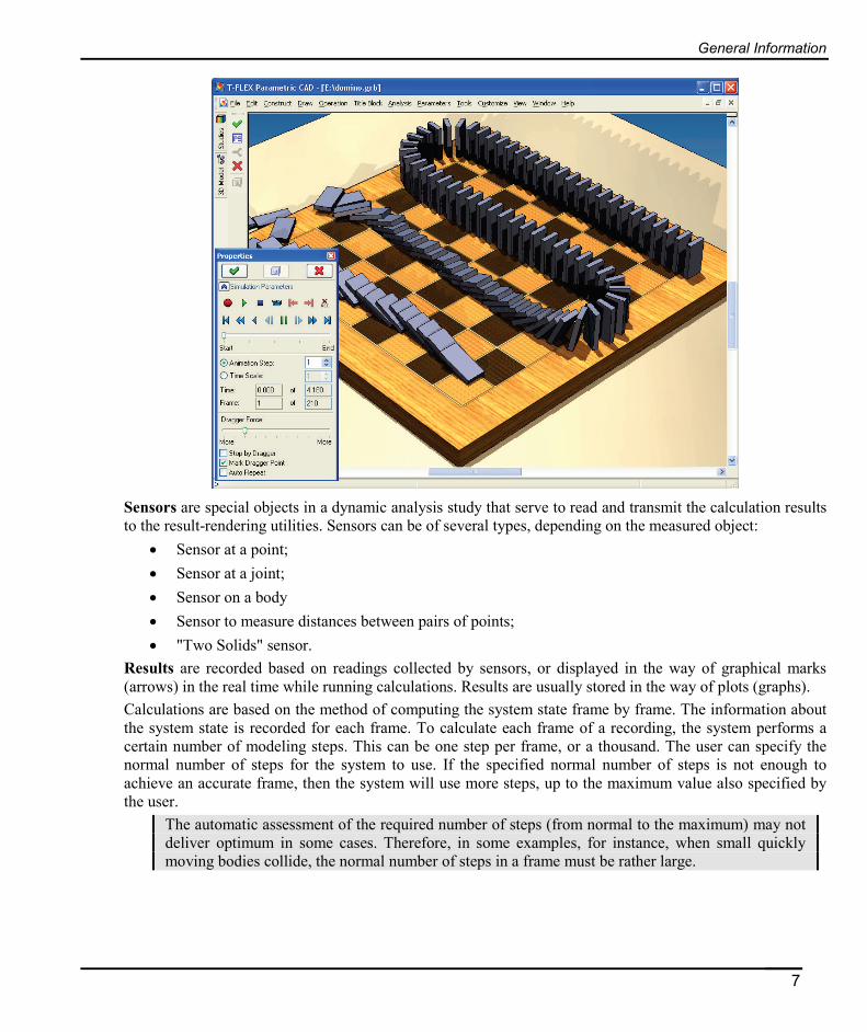
Sensors are special objects in a dynamic analysis study that serve to read and transmit the calculation results to the result-rendering utilities. Sensors can be of several types, depending on the measured object:

• Sensor at a point; • Sensor at a joint; • Sensor on a body • Sensor to measure distances between pairs of points; • "Two Solids" sensor.

Results are recorded based on readings collected by sensors, or displayed in the way of graphical marks (arrows) in the real time while running calculations. Results are usually stored in the way of plots (graphs). Calculations are based on the method of computing the system state frame by frame. The information about the system state is recorded for each frame. To calculate each frame of a recording, the system performs a certain number of modeling steps. This can be one step per frame, or a thousand. The user can specify the normal number of steps for the system to use. If the specified normal number of steps is not enough to achieve an accurate frame, then the system will use more steps, up to the maximum value also specified by the user.

The automatic assessment of the required number of steps (from normal to the maximum) may not deliver optimum in some cases. Therefore, in some examples, for instance, when small quickly moving bodies collide, the normal number of steps in a frame must be rather large.

7


Rules of Performing Dynamic Calculations Dynamic calculations are based on a special system object – a dynamic analysis study. The study unites data and elements required for running specific calculations of a model. It contains the data that define the direction of gravity, the default properties of the study elements (joint properties, friction forces, contact properties), the time factor in the modeled process, as well as the information about the used bodies, loads, and properties of relations between individual components, etc. After completing the calculations, the study will also include the calculation results. A dynamic analysis study is associatively related with the 3D model. As some parameters or contents of the model change, the study would automatically adjust.

Study Management Utilities To display the list of a model's studies, there is a special "Studies" window. It contains the portion of the current model tree, which represents the contents of the engineering analysis studies (similar functions are provided in the "3D model" tool window. The window provides a quick access to elements of each study. Dynamic Analysis study elements (joints, loads, sensors, results) are arranged into groups. The studies tool window is common for the studies in the finite element and in the dynamic analysis. The command to open this window is called as follows:

Keyboard Textual Menu Icon

<3MW> "Analysis|Show Studies Window"

Similar to other types of engineering studies that can be contained in a T-FLEX CAD model (finite element studies), it is possible to have several dynamic analysis studies in one file. Each of the studies may contain its own set of elements and boundary conditions in order to find solutions in different formulations or under different loads. Most of study management commands are available in the context menu that can be accessed in this window. The study currently being worked on is called active. The active study's icon has a red check in the studies window. To make another study active, use the context menu command "Activate".

The "Update" command is available in the context menu of the selected Study. It is used to quickly refresh the study data after making changes to the model, if the full recalculation was skipped. To a get a study or to modify its properties, use the commands "Edit" and "Properties".

A special command is provided for managing the list of studies:


"Analysis|Studies..."

8

Rules of Performing Dynamic Calculations

The dialog window of this command displays the list of all studies existing in the current document. This window is common for both the dynamic analysis studies and finite element analysis. The buttons for calling the main commands are to the right of the list. The export, copying and material property definition commands are not available in the dynamic analysis case.

If several studies are created in the system, only one of them will be active. New elements are created, and calculations are run, only in the active study.

Creating Study To create a new Dynamic Analysis study, use the command:


<3MN> "Analysis|New Study|Dynamic Analysis"

This command allows creating two types of studies – "Express Dynamic Analysis" and "Dynamic Analysis". The Express Analysis is shipped free together with the T-FLEX CAD 3D program and has certain limitations. The limitations on the Express module are reviewed in a separate paragraph of this chapter. Upon calling the study creation command, the following options become available in the automenu:

 Set entity Parameters

<S> Select Solids of dynamic analysis

<R> Select Solids used in contact analysis

<C> Select the bodies to set contact parameters

A study can be created "as is", based on the data of the 3D model. To create

such a study, you can just click in the properties window or in the automenu. Contact between bodies is ignored by default (whereas the friction is accounted for by default). The necessary number of joints is automatically created, based on the mates and degrees of freedom in the 3D model. The study's properties window has numerous parameters to allow for a precise study setup. For the user's convenience, the window is arranged into blocks.

In the [Solids] block of parameters, the user can manually specify the model Solids that shall be included in the dynamic analysis study. This setting is needed in the case when the model has more bodies than required for calculations. This also saves the computational resources, by excluding insignificant objects from calculations.

9


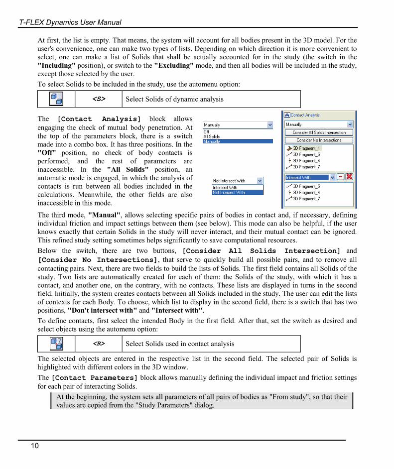
At first, the list is empty. That means, the system will account for all bodies present in the 3D model. For the user's convenience, one can make two types of lists. Depending on which direction it is more convenient to select, one can make a list of Solids that shall be actually accounted for in the study (the switch in the "Including" position), or switch to the "Excluding" mode, and then all bodies will be included in the study, except those selected by the user. To select Solids to be included in the study, use the automenu option:

<S> Select Solids of dynamic analysis

The [Contact Analysis] block allows engaging the check of mutual body penetration. At the top of the parameters block, there is a switch made into a combo box. It has three positions. In the "Off" position, no check of body contacts is performed, and the rest of parameters are inaccessible. In the "All Solids" position, an automatic mode is engaged, in which the analysis of contacts is run between all bodies included in the calculations. Meanwhile, the other fields are also inaccessible in this mode.

The third mode, "Manual", allows selecting specific pairs of bodies in contact and, if necessary, defining individual friction and impact settings between them (see below). This mode can also be helpful, if the user knows exactly that certain Solids in the study will never interact, and their mutual contact can be ignored. This refined study setting sometimes helps significantly to save computational resources. Below the switch, there are two buttons, [Consider All Solids Intersection] and [Consider No Intersections], that serve to quickly build all possible pairs, and to remove all contacting pairs. Next, there are two fields to build the lists of Solids. The first field contains all Solids of the study. Two lists are automatically created for each of them: the Solids of the study, with which it has a contact, and another one, on the contrary, with no contacts. These lists are displayed in turns in the second field. Initially, the system creates contacts between all Solids included in the study. The user can edit the lists of contexts for each Body. To choose, which list to display in the second field, there is a switch that has two positions, "Don't intersect with" and "Intersect with". To define contacts, first select the intended Body in the first field. After that, set the switch as desired and select objects using the automenu option:

<R> Select Solids used in contact analysis

The selected objects are entered in the respective list in the second field. The selected pair of Solids is highlighted with different colors in the 3D window. The [Contact Parameters] block allows manually defining the individual impact and friction settings for each pair of interacting Solids.

At the beginning, the system sets all parameters of all pairs of bodies as "From study", so that their values are copied from the "Study Parameters" dialog.

10


To define individual contact parameters between two Solids, such a pair shall first be selected in the fields of the properties window. The first Body is selected in the upper field. The lower field will then display the list of all Solids, with which the first one may, or, alternatively, may not, contact. You select the second Body from the latter list. The selected objects are highlighted with different colors in the 3D window. After selecting a pair, you can define its individual contact properties at the lower part of the properties window. There is an alternative way to select pairs, where you can select Solids directly in the 3D window. The following automenu options will help doing this. Once you click the option,

<C> Select the bodies to set contact parameters

the system goes into the mode of defining individual contact parameters, and two additional options appear in the automenu to select the first and the second Body:

<F> Select first Solid

<G> Select second Solid

These options activate in turns. The selected objects are marked with different colors in the 3D window.

Study Parameters

The option calls the dialog to define the time characteristics and accuracy of parameters of a calculation, as well as a geometrical properties of certain objects in the current dynamic analysis study. The same dialog can be called by clicking the [Parameters] button in the properties window. The dialog has three tabs. On the [Basic] tab you can define (or modify when you edit) the name of the dynamic analysis study. The "Modeling time" group of interface controls defines the time-related parameters and the modeling step for calculating the current study. These parameters can be defined in two ways. You can define the overall duration and the number of frames per second, or define the duration of one frame and the total number of frames.

Time-related parameters can be modified in the calculation parameters just before starting calculations.

The group of parameters "Steps per frame" defines the number of iterations found by the system to find the solution for each frame. There are two parameters: the first one indicates the normal number of steps to find the precise solution, whereas the

11


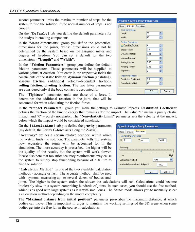
second parameter limits the maximum number of steps for the system to find the solution, if the normal number of steps is not enough.

On the [Default] tab you define the default parameters for the study's interacting components. In the "Joint dimensions" group you define the geometrical dimensions for the joints, whose dimensions could not be determined by the system based on the assigned mates and degrees of freedom. You can set a default for the two dimensions - "Length" and "Width". In the "Friction Parameters" group you define the default friction parameters. Those parameters will be supplied to various joints at creation. You enter in the respective fields the coefficients of the static friction, dynamic friction (at sliding), viscous friction (additional velocity-dependent friction), rolling friction, pivoting friction. The two latter parameters are considered only if the body contact is accounted for. The "Tightness" parameter units are those of a force. It determines the additional reaction in the joint, that will be accounted for when calculating the friction forces. In the "Impact Parameters" group you make the settings to evaluate impacts. Restitution Coefficient defines the fraction of the kinetic energy that remains after the impact. The value "1" means a purely elastic impact, and "0" – purely nonelastic. The "Non-elasticity Limit" parameter sets the velocity at the impact, below which the impact would be considered nonelastic. On the [Simulation] tab you define the gravity parameters (my default, the Earth's G-force acts along the Z-axis). "Accuracy" defines a certain relative corridor, within which the system finds the solution. The parameter tells the system, how accurately the joints will be accounted for in the simulation. The more accuracy is prescribed, the higher will be the quality of the results, but the system will work slower. Please also note that too strict accuracy requirements may cause the system to simply stop functioning because of a failure to find the solution. "Calculation Method" is one of the two available calculation methods - accurate or fast. The accurate method shall be used with systems measuring up to several dozen of bodies and

joints. The higher is the system order, the slower the calculations will run. Calculations could become intolerably slow in a system comprising hundreds of joints. In such cases, you should use the fast method, which is as good with large systems as it is with small ones. The "Auto" mode allows you to manually select a calculation method depending on the model complexity. The "Maximal distance from initial position" parameter prescribes the maximum distance, at which bodies can move. This is important in order to maintain the working settings of the 3D scene when some bodies get into the free fall in the course of calculations.

12


Joints Joints are created automatically at the time of the study creation, based on the mates and the specified degrees of freedom of the 3D model elements. As you make changes to the model's mates, the set of joints will change when the study is updated. The user can additionally adjust the mechanical properties by defining friction parameters. The set of properties may differ, depending on the joint type. The following table comprises the settings that can be adjusted, for all joint types.

Joint type Geometrical parameters Friction and impact parameters

Spherical joint

• Radius • Static friction • Dynamic friction • Viscous friction • Tightness

Rotational joint

• Radius • Length • Displacement

• Static friction • Dynamic friction • Viscous friction • Tightness

Translational joint

• Length • Width • Thickness • Rotation • Displacement


Cylindrical joint

• Radius • Length • Displacement


Helical joint

• Radius • Static friction • Dynamic friction • Viscous friction • Tightness

Contact-type joint

absent • Restitution Coefficient • Non-elasticity limit • Static friction • Dynamic friction • Pivoting Friction • Rolling Friction

Generic joint absent absent

13


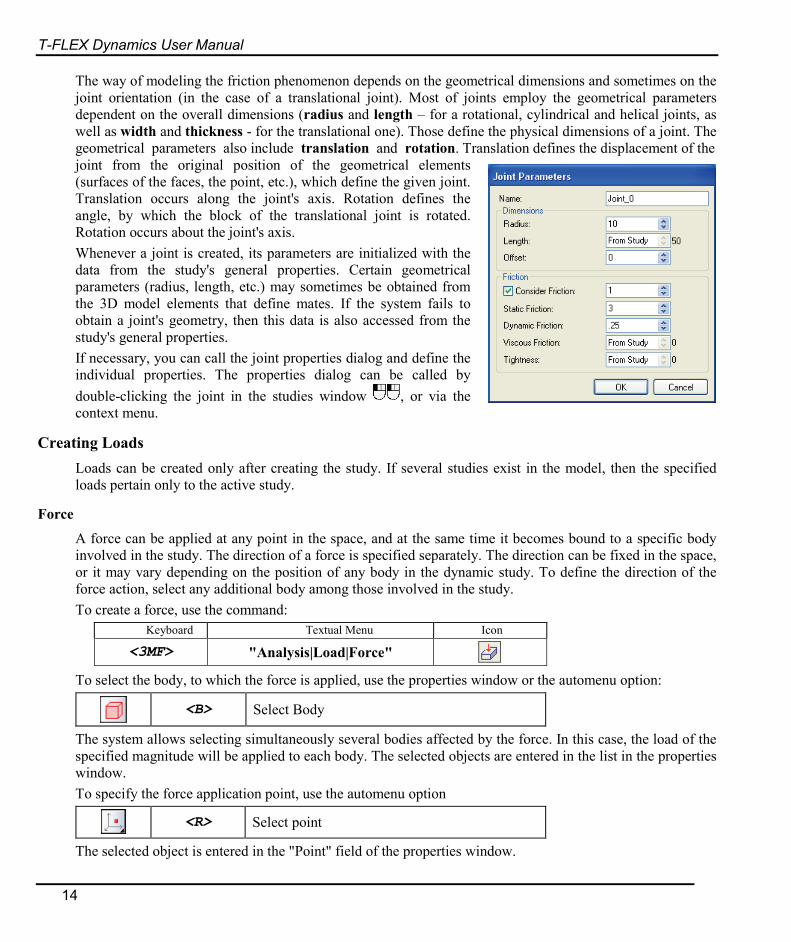
The way of modeling the friction phenomenon depends on the geometrical dimensions and sometimes on the joint orientation (in the case of a translational joint). Most of joints employ the geometrical parameters dependent on the overall dimensions (radius and length – for a rotational, cylindrical and helical joints, as well as width and thickness - for the translational one). Those define the physical dimensions of a joint. The geometrical parameters also include translation and rotation. Translation defines the displacement of the joint from the original position of the geometrical elements (surfaces of the faces, the point, etc.), which define the given joint. Translation occurs along the joint's axis. Rotation defines the angle, by which the block of the translational joint is rotated. Rotation occurs about the joint's axis. Whenever a joint is created, its parameters are initialized with the data from the study's general properties. Certain geometrical parameters (radius, length, etc.) may sometimes be obtained from the 3D model elements that define mates. If the system fails to obtain a joint's geometry, then this data is also accessed from the study's general properties. If necessary, you can call the joint properties dialog and define the individual properties. The properties dialog can be called by double-clicking the joint in the studies window , or via the context menu.

Creating Loads Loads can be created only after creating the study. If several studies exist in the model, then the specified loads pertain only to the active study.

Force

A force can be applied at any point in the space, and at the same time it becomes bound to a specific body involved in the study. The direction of a force is specified separately. The direction can be fixed in the space, or it may vary depending on the position of any body in the dynamic study. To define the direction of the force action, select any additional body among those involved in the study. To create a force, use the command:


<3MF> "Analysis|Load|Force"

To select the body, to which the force is applied, use the properties window or the automenu option:

 Select Body

The system allows selecting simultaneously several bodies affected by the force. In this case, the load of the specified magnitude will be applied to each body. The selected objects are entered in the list in the properties window. To specify the force application point, use the automenu option

<R> Select point

The selected object is entered in the "Point" field of the properties window.

14


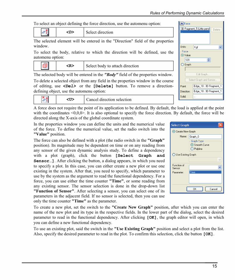
To select an object defining the force direction, use the automenu option:

<D> Select direction

The selected element will be entered in the "Direction" field of the properties window. To select the body, relative to which the direction will be defined, use the automenu option:

<R> Select body to attach direction

The selected body will be entered in the "Body" field of the properties window. To delete a selected object from any field in the properties window in the course of editing, use <Del> or the [Delete] button. To remove a direction-defining object, use the automenu option:

 Cancel direction selection

A force does not require the point of its application to be defined. By default, the load is applied at the point with the coordinates <0,0,0>. It is also optional to specify the force direction. By default, the force will be directed along the X-axis of the global coordinate system. In the properties window you can define the units and the numerical value of the force. To define the numerical value, set the radio switch into the "Value" position. The force can also be defined with a plot (the radio switch in the "Graph" position). Its magnitude may be dependent on time or on any reading from any sensor of the given dynamic analysis study. To define a dependency with a plot (graph), click the button [Select Graph and Sensor…]. After clicking the button, a dialog appears, in which you need to specify a plot. In this case, you can either create a new plot or use one existing in the system. After that, you need to specify, which parameter to use by the system as the argument to read the functional dependency. For a force, you can use either the time counter "Time", or some reading from any existing sensor. The sensor selection is done in the drop-down list "Function of Sensor". After selecting a sensor, you can select one of its parameters in the adjacent field. If no sensor is selected, then you can use only the time counter "Time" as the parameter.

To create a new plot, set the switch to the "Create New Graph" position, after which you can enter the name of the new plot and its type in the respective fields. In the lower part of the dialog, select the desired parameter to read in the functional dependency. After clicking [OK], the graph editor will open, in which you can define a new functional dependency. To use an existing plot, said the switch in the "Use Existing Graph" position and select a plot from the list. Also, specify the desired parameter to read in the plot. To confirm this selection, click the button [OK].

15


The name of the plot will appear in the special field of the main properties window, with the driving parameter entered next in parentheses. There will be also the button [Edit Graph], with which you can call the graph editor to modify the functional dependency.

Example of defining a variable force via a plot

Rotation

The "Rotation" load allows to create an external force that rotates the selected body with a constant angular velocity about the specified axis. You can specify the maximum moment as the limit that cannot be exceeded by the "Rotation" load, with the force ceasing for the duration of the countering moment action. To create a rotation, use the command:


<3MR> "Analysis|Load|Rotation"

To select the body, to which the load is applied, use the properties window or the automenu option:

 Select Solid Body

The system allows selecting several bodies simultaneously. In this case, the load of the specified magnitude will be applied to each of them. The selected objects are entered in the list in the properties window. The rotation direction (as a vector) is defined using the following automenu option:

<A> Select axis of revolution

To define the axis, you can select any 3D object suitable for defining a direction. The selected element will be entered in the "Axis of Rotation" field of the properties window. The rotation direction can be related (bound) to any movable or still body in the

16


study, using the automenu option:

<R> Select solid to define direction

The selected body is entered in the respective field of the properties window, and the "Axis is attached to Body" option becomes active. The numerical value of the angular velocity and the units are defined in the properties window. You can select the measurement units in the adjacent list. If necessary, you can additionally specify the value of the maximum torque (moment). If you do not need to limit the moment, then disable the option "Limited Torque".

Torque

This type of load simulates a moment applied to the selected body or set of bodies. To create a moment, use the command:


<3MQ> "Analysis|Load|Torque"



The system allows selecting several bodies simultaneously. In this case, the load of the specified magnitude will be applied to each of them. The selected objects are entered in the list in the properties window. The moment (torque) application direction (as a vector) is defined using the following automenu option:

<A> Click to select direction

The selected element will be entered in the "Axis of Rotation" field of the properties window. The torque value and the units are defined in the properties window. The torque value can be defined with a plot. For example, you can define a dependency of the torque on the angular velocity, using the sensor that is measuring the angular velocity. The steps to define the plot for the torque are fully identical to the steps described for the "Force" load type.

Initial Velocity

The "Initial Velocity" load type creates an initial impulse applied to the selected body. To create the initial velocity, use the command:


<3MV> "Analysis|Load|Initial Velocity"



17


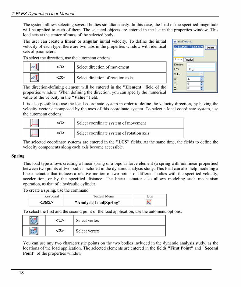
The system allows selecting several bodies simultaneously. In this case, the load of the specified magnitude will be applied to each of them. The selected objects are entered in the list in the properties window. This load acts at the center of mass of the selected body. The user can create a linear or angular initial velocity. To define the initial velocity of each type, there are two tabs in the properties window with identical sets of parameters. To select the direction, use the automenu options:

<D> Select direction of movement

<D> Select direction of rotation axis

The direction-defining element will be entered in the "Element" field of the properties window. When defining the direction, you can specify the numerical value of the velocity in the "Value" field.

It is also possible to use the local coordinate system in order to define the velocity direction, by having the velocity vector decomposed by the axes of this coordinate system. To select a local coordinate system, use the automenu options:

<С> Select coordinate system of movement

<C> Select coordinate system of rotation axis

The selected coordinate systems are entered in the "LCS" fields. At the same time, the fields to define the velocity components along each axis become accessible.

Spring

This load type allows creating a linear spring or a bipolar force element (a spring with nonlinear properties) between two points of two bodies included in the dynamic analysis study. This load can also help modeling a linear actuator that induces a relative motion of two points of different bodies with the specified velocity, acceleration, or by the specified distance. The linear actuator also allows modeling such mechanism operation, as that of a hydraulic cylinder. To create a spring, use the command:


<3MG> "Analysis|Load|Spring"

To select the first and the second point of the load application, use the automenu options:

<1> Select vertex

<2> Select vertex

You can use any two characteristic points on the two bodies included in the dynamic analysis study, as the locations of the load application. The selected elements are entered in the fields "First Point" and "Second Point" of the properties window.

18


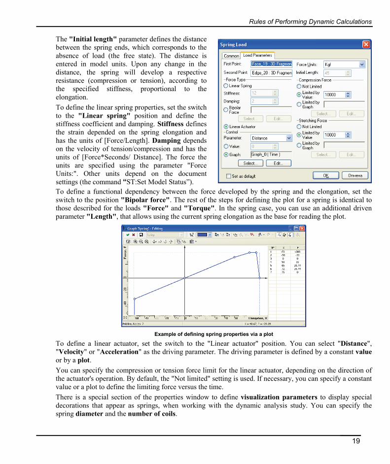
The "Initial length" parameter defines the distance between the spring ends, which corresponds to the absence of load (the free state). The distance is entered in model units. Upon any change in the distance, the spring will develop a respective resistance (compression or tension), according to the specified stiffness, proportional to the elongation. To define the linear spring properties, set the switch to the "Linear spring" position and define the stiffness coefficient and damping. Stiffness defines the strain depended on the spring elongation and has the units of [Force/Length]. Damping depends on the velocity of tension/compression and has the units of [Force*Seconds/ Distance]. The force the units are specified using the parameter "Force Units:". Other units depend on the document settings (the command “ST:Set Model Status”). To define a functional dependency between the force developed by the spring and the elongation, set the switch to the position "Bipolar force". The rest of the steps for defining the plot for a spring is identical to those described for the loads "Force" and "Torque". In the spring case, you can use an additional driven parameter "Length", that allows using the current spring elongation as the base for reading the plot.

Example of defining spring properties via a plot

To define a linear actuator, set the switch to the "Linear actuator" position. You can select "Distance", "Velocity" or "Acceleration" as the driving parameter. The driving parameter is defined by a constant value or by a plot. You can specify the compression or tension force limit for the linear actuator, depending on the direction of the actuator's operation. By default, the "Not limited" setting is used. If necessary, you can specify a constant value or a plot to define the limiting force versus the time. There is a special section of the properties window to define visualization parameters to display special decorations that appear as springs, when working with the dynamic analysis study. You can specify the spring diameter and the number of coils.

19


Creating Sensors Sensors can be created only for the active study of the dynamic or strength analysis, using the command:


<3MD> "Analysis|Sensor"

In the properties window you can specify the type of the sensor being created. Body. This sensor serves to measure coordinates, linear and angular velocities and accelerations, as well as the equivalent force and torque (moment) acting on the body. The equivalent force or moment is the sum of all external loads applied to the body.

Point. This sensor serves to measure coordinates, linear velocities and accelerations of any point of the mechanical system. Joint. This sensor serves to measure the reaction forces and moments in a joint, friction forces, velocities, acceleration and coordinates of a joint. You select one of the study's joints as the object to host the sensor. Distance. This sensor can read the distance between two points connected to the arbitrary bodies of the study, the velocity, with which a distance changes, and acceleration. You select two model points as the base objects to create this sensor. Additionally, for each of the points you select a body in the study, with which it moves together, as the mechanical system moves. Two Solids. This sensor serves to measure the reaction and friction forces at the contact of two bodies. You select two bodies of the study as the base of the sensor creation. After calling the sensor creation command, various options appear in the automenu to help selecting objects. The set of options depends on the type of the sensor being created:


<V> Select point

<C> Cancel Selection

In the properties window, there is a collection of fields (Operation, Element, Second Operation, Second Element), in which the names of the selected object appear. In the "Visualize" section, you can customize the display of auxiliary graphics objects, that will the outputting certain sensor readings during the calculation process (see the table below).

Parameter Drawing Style Sensor Trajectory 3D curve Point, Body, Joint, Reaction force Vector Joint, a pair of bodies Reaction moment Vector Joint, a pair of bodies Friction force Vector Joint, a pair of bodies Friction moment Vector Joint, a pair of bodies

20


Linear velocity Vector Body Angular velocity Vector Body Linear acceleration Vector Body Angular acceleration Vector Body Action force Vector Body Action moment Vector Body Velocity Vector Point Acceleration Vector Point

Explanations to the table: 1) For the "Two Solids" sensor, the coordinates are computed, and then the trajectory is displayed of the point that is the center of the contact area between the two bodies. 2) For the "Joint" sensor, the coordinates of the joint center are computed.

You can define the scale and color settings for the graphics objects that appear as a vector arrow. For a trajectory, you can specify the color and, if necessary, limit the curve length by specifying a fixed number of last calculated points for it. Sensors are displayed in the 3D window as spherical-shape graphics objects.

Creating Results. Result Types You can create a plot in the dynamic analysis study as a record of readings obtained from a sensor. The plot that represents the readings of some sensor in the dynamic analysis study is called a result. The result creation command can be called in several ways: 1. From the context menu of the sensor selected in the 3D model tree or in the studies window. 2. In the text menu or by typing on the keyboard:


<3MZ> "Analysis|Result"

21


The command is accessible, if there is at least one sensor. After calling the command, the result creation dialog appears. The result is created based on the readings of a particular sensor, whose set depends on the sensor type. The set of reading types can be viewed in the compendium table of the "Creating sensors" topic (please see above). Additionally, when creating a plot, it is possible to extract the X,Y,Z – components as separate results for each reading. In the "Sensor" combo box, you select a sensor among those existing in the study. In the "Values" field, set the checks against the readings, based on which you need to create results. Once the marks are set and the dialog is closed, the system creates new objects of the "Graph" type, which are populated with the data after finishing the study calculation.

The new plots receive the names according to the sensor name and the reading on which they are based. Such plots have the "Read Only" system attribute and the "Polyline" type. You can view those outside the dynamic analysis study, using the regular tools to work with plots/graphs (see the chapter "Graphs").

Running Calculations The command of running the calculations can be launched in several ways:

1. From the context menu of the study selected in the 3D model tree or in the studies window. 2. In the text menu or by typing on the keyboard:


<3MY> "Analysis|Solve" After calling the command, the system goes into the mode of waiting for the result of the calculations or rendering the calculated results. The parameters to control the process and view the results appear in the properties window. This command can work in two modes – in the mode of calculating, or in the mode of viewing the ready results. Upon the first launch of the "calculation" command, the system doesn't have any results yet. You can judge that by the inaccessible buttons to view the results. At this point, you can only start new calculations. You control the calculations process via the properties window, in which there are necessary control elements.

Record

Starts the calculations. Upon an attempt to start new calculations whenever there are previously obtained results, the system will warn you with a query.

22


Play Starts the playback of the calculation results. The button is accessible if there are saved results of calculations.

Stop Stops the calculation process or the results playback.

Create AVI File Starts the mode of recording a video clip at the time of playing back results. When results are played back, each video frame captures the current image of the 3D scene at the respective instance of the playback. Immediately during the calculations or the results playback, the user can arbitrarily spin the 3D scene or use any existing cameras for the view. When the clip-recording button is clicked, the standard "Animation" dialog is displayed to set up the video recording parameters (for details, see the chapter "Animation").

Trim Left

Trim Right

These buttons clip the record of the saved result at the current playback instant. The options are used to remove unnecessary fragments of the recording.

Delete Record This button serves to delete the saved results before running new calculations.

The saved calculations render the model behavior in the state in which it was back at the moment of calculating the results. If changes are introduced in the model that need to be accounted for in calculation (for example, it could be the changes in the properties/number of joints, load

parameters, study conditions, etc.), then you shall delete the saved results using the option , and then start a new calculation with the button .

Below in the properties window there is another pane with the buttons to rewind, search for a particular time instant, and play back the results of a dynamic calculation.

To Start

Rewind

Playback

Previous Frame

Pause

Next

Fast Forward

To End

23


Below the panes that control the calculation, there is a special slider, that allows setting the time counter to any instant. A scale with time intervals appears on the slider bar as the total time increases. By using the "Animation Step" parameter, you can set the speed of the result playback. You can use only the integer numbers here. In fact, this parameter sets the step to pick the frames from the array of results. It can be conveniently used when creating animated clips in the real time, if the calculations were run with a large number of frames per second in order to obtain quality results. An alternative way to control the playback speed is provided by the parameter "Time Scale". Displayed below are the time parameter for each frame and the frame counter. When the calculations run, the user can grab any movable part with the cursor and act on it with a relative force, which depends on the distance to the grabbing point and on the "Dragger Force" parameter setting. To grab, you make a

pause with . Next, while holding down the left mouse button, you need to "pull" the part in the desired direction. "Dragger Force" – this is a special control element that sets a relative dragger force to act on the model while running calculations. Stop by Dragger. This option automatically pauses the calculations process each time when the dragger is engaged. It is convenient to use whenever the dynamic calculation is conducted with additional loads imposed by the dragger, and the instants must be excluded when the model is off the dragger. Mark Dragger Point. This option enables the display of a crosshair mark which denotes the application point of the dragger force. Auto Repeat. This option turns on an automatic replay loop. Whenever there are results in the study, the "Show Results" section appears in the properties window, that contains the list of all plots created in the study. There is a switch before each element, which controls the display in the course of calculations. When calculations are run, each plot is displayed in a separate floating window. The curve in the plot is automatically extended as more calculated data become available. Each floating plot window has the plot management functions analogous to those in the standard graph editor. The plot images in each window are automatically scaled in order to continuously display the active area. Plots are also displayed when the results are played back. To mark the current time instant, a special pointer dynamically moves in each graph's "Argument Marker". The user can adjust the size of the floating windows and the plot display scale as desired. If necessary, each plot can be inspected in detail in the special graph editor. Detailed information on working with plots/graphs can be found in the chapter "Graphs". When running calculations, it may often be necessary to set different intervals for the time counter, and different modeling parameters. In the automenu there is the option to call the dialog for managing some general study parameters. This dialog duplicates the respective portions of the general study settings dialog (see above) and has two tabs, [Basic] and [Simulation]. It helps quickly access the necessary study settings directly in the calculation running command. For example, the group of parameters "Steps per

24

Limitations of the Express Dynamics Analysis Module

frame" control is the number of calculation steps. The calculation speed and accuracy depend on these settings. Sometimes, when running preliminary trial calculations, one may need to set a higher speed at the expense of the accuracy.

Limitations of the Express Dynamics Analysis Module 1. The utilities to read numerical results are limited. Plots are not output. 2. The capability of animation clip generation is restricted.

25

Documents

T-FLEX Dynamics - SoliCAD.comsolicad.com/media/download/tflex/manual/tflex_dynamics_um.pdf · T-FLEX Dynamics User Manual General Information The dynamic analysis module is integrated