Embed Size (px)
Citation preview
Topological Parameters for Time-Space Tradeo�
Rina Dechter
Information & Computer Science, University of California, Irvine, CA [email protected]
Yousri El Fattah
Rockwell Science Center, 1049 Camino Dos Rios, Thousand Oaks, CA [email protected]
3 June 1999
Abstract
In this paper we propose a family of algorithms combining tree-clustering withconditioning that trade space for time. Such algorithms are useful for reasoningin probabilistic and deterministic networks as well as for optimization tasks. Byanalyzing the problem structure the user can select from a spectrum of hybrid algo-rithms, the one that best meets a given time-space speci�cation. To determine thepotential of this approach, we analyze the structural properties of problems com-ing from the circuit diagnosis domain. The analysis demonstrate how the tradeo�sassociated with various hybrids can be explicated and be used for each probleminstance.
1 Introduction
Problem solving methods can be viewed as hybrids of two main principles:inference and search. Inference algorithms are time and space exponentialin the size of the relationships they record while search algorithms are timeexponential but require only linear memory. In this paper we develop a hybridscheme that uses inference (tree-clustering) and search (conditioning) as itstwo extremes and, using a single structure-based design parameter, permitsthe user to control the storage-time tradeo� in accordance with the applicationand the available resources.
In general, topology-based algorithms for constraint satisfaction and proba-bilistic reasoning fall into two distinct classes. One class is centered on tree-clustering, the other on cycle-cutset decomposition. Tree-clustering involves
Preprint submitted to Elsevier Science 3 June 1999
transforming the original problem into a tree-like problem that can then besolved by a specialized e�cient tree-solving algorithm [1,2]. The transformingalgorithm identi�es subproblems that together form a tree, and the solutionsto the subproblems serve as the new values of variables in a tree metalevelproblem. The metalevel problem is called a join-tree. The tree-clustering algo-rithm is time and space exponential in the tree-width of the problem's graph.A related parameter is the induced-width which equals the tree-width minusone. We will use both terms interchangeably.
The cycle-cutset method, also called loop-cutset conditioning, utilizes the prob-lem's structure in a di�erent way. It exploit the fact that variable instantiationchanges the e�ective connectivity of the underlying graph. A cycle-cutset ofan undirected graph is a subset of its nodes which, once removed, cuts allof the graph's cycles. A typical cycle-cutset method enumerates the possibleassignments to a set of cutset variables and, for each cutset assignment, solves(or reasons about) a tree-like problem in polynomial time. Thus, the overalltime complexity is exponential in the size of the cycle-cutset [3]. Fortunately,enumerating all the cutset's assignments can be accomplished in linear space,yielding an overall linear space algorithm.
The �rst question is which method, tree-clustering or the cycle-cutset schemeprovide a better worst-case time guarantees. This question was answered byBertele and Briochi [4] in 1974 and later rea�rmed in [5]. They showed that,the minimal cycle-cutset of any graph can be much larger, and is never smallerthan its minimal tree-width. In fact, for an arbitrary graph, r � c, where cis the minimal cycle-cutset and r is the tree-width [4]. Consequently, for anyproblem instance the time guarantees accompanying the cycle-cutset schemeare never tighter than those of tree-clustering, and can be even much worse.On the other hand, while tree-clustering requires exponential space (in theinduced-width) the cycle-cutset requires only linear space.
Since the space complexity of tree-clustering can severely limit its usefulness,we investigate in this paper the extent to which space complexity can bereduced, while reasonable time complexity guarantees are maintained. Is itpossible to have the time guarantees of clustering while using linear space?On some problem instances, it is possible. Speci�cally, on those problemswhose associated graph has an induced width and a cycle-cutset of comparablesizes (e.g., on a ring, the cutset size is 1 and the tree width is 2, leading toidentical time bounds). We conjecture, however, that any algorithm that has atime bound guarantee exponential in the induced-width will, on some probleminstances, require exponential space in the induced width.
The space complexity of tree-clustering can be bounded more tightly usingthe separator width, which is de�ned as the size of the maximum subset ofvariables shared by adjacent subproblems in the join-tree. Our investigation
2

employs the separator width to control the time-space tradeo�. The idea isto combine adjacent subproblems joined by a large separator into one biggercluster or subproblem so that the remaining separators are of smaller size.Once a join-tree with smaller separators is generated, its potentially largerclusters can be solved using the cycle-cutset method, or any other linear-spacescheme.
In this paper we will develop a time-space tradeo� scheme that is applicableto belief network processing, constraint processing, and optimization tasks,yielding a sequence of parametrized algorithms that can trade space for time.With this scheme it will be possible to select from a spectrum of algorithms theone that best meets some time-space requirement. Algorithm tree-clusteringand cycle-cutset conditioning are two extremes in this spectrum.
We investigate the potential of our scheme in the domain of combinatorial cir-cuits. This domain is frequently used as an application area in both probabilis-tic and deterministic reasoning [6{8]. We analyze 11 benchmark combinatorialcircuits widely used in the fault diagnosis and testing community [9] (see Ta-ble 1 ahead.). For each circuit, the analysis is summarized in a chart displayingthe time-space complexity tradeo�s for diagnosing that circuit. The analysisallows tailoring the hybrid of tree-clustering and cycle-cutset decompositionto the available memory.
In order to demonstrate our claims we use a directional variant of tree-cluteringthat is query-based which simplify the exposition. However, the approach isapplicable to the general version of tree-clustering.
Section 2 gives de�nitions and preliminaries and introduces the time-spacetradeo� ideas using belief networks. Sections 3 and 4 extends these ideas toconstraint networks and to optimization problems. Section 5 describes theempirical framework and Section 6 presents the results. Section 7 discussesrelated works and section 8 gives our conclusion.
The paper assumes familiarity with the basic concepts of tree-clustering andcycle-cutset conditioning and provides only breif necessary background. Formore details the reader should consult the references.
3
2 Probabilistic Networks
2.1 Overview
2.1.1 De�nitions and notations
Belief networks provide a formalism for reasoning about partial beliefs underconditions of uncertainty. It is de�ned by a directed acyclic graph over nodesrepresenting random variables of interest (e.g., the temperature of a device, thegender of a patient, a feature of an object, the occurrance of an event). The arcssignify the existence of direct causal in uences between the linked variables.The strength of these in uences are quanti�ed by conditional probabilitiesthat are attached to each cluster of parents-child nodes in the network. Abelief network is a concise description of a complete probability distribution.It uses the concept of a directed graph.
De�nition 1 (Directed graph) A directed graph G = fV;Eg, where V =fX1; :::;Xng is a set of elements and E = f(Xi;Xj)jXi;Xj 2 V g is the setof edges. If an arc (Xi;Xj) 2 E, we say that Xi points to Xj . For eachvariable Xi, pa(Xi) is the set of variables pointing to Xi in G, while ch(Xi)is the set of variables that Xi points to. The family of Xi includes Xi and itsparent variables. A directed graph is acyclic if it has no directed cycles. In anundirected graph the direction of the arcs is ignored: (Xi;Xj) and (Xj;Xi) areidentical. An undirected graph is chordal if every cycle of length 4 has a chord.A clique is a subgraph that is completely connected and a maximal clique ofgraph is a clique that is not contained in any other clique of the graph.
De�nition 2 (Belief Networks) Let X = fX1; :::;Xng be a set of ran-dom variables over multi-valued domains, D1; :::;Dn. A belief network is apair (G;P ) where G is a directed acyclic graph over the nodes X and P =fPig are the conditional probability matrices over the families of G, Pi =fP (Xijpa(Xi)g. An assignment (X1 = x1; :::;Xn = xn) can be abbreviated asx = (x1; :::; xn). The belief network represents a probability distribution overX having the product form
P (x1; ::::; xn) = �ni=1P (xijxpa(Xi))
where xpa(Xi) denotes the projection of a tuple x over pa(Xi). An evidence sete is an instantiated subset of variables. A moral graph of a belief network is anundirected graph generated by connecting the tails of any two head-to-headpointing arcs in G and removing the arrows. A belief network is a polytree ifits underlying undirected (unmoralized) graph has no cycles (namely, it is atree).
4

A
B
CD E
FG
H A
B
CD E
FG
H
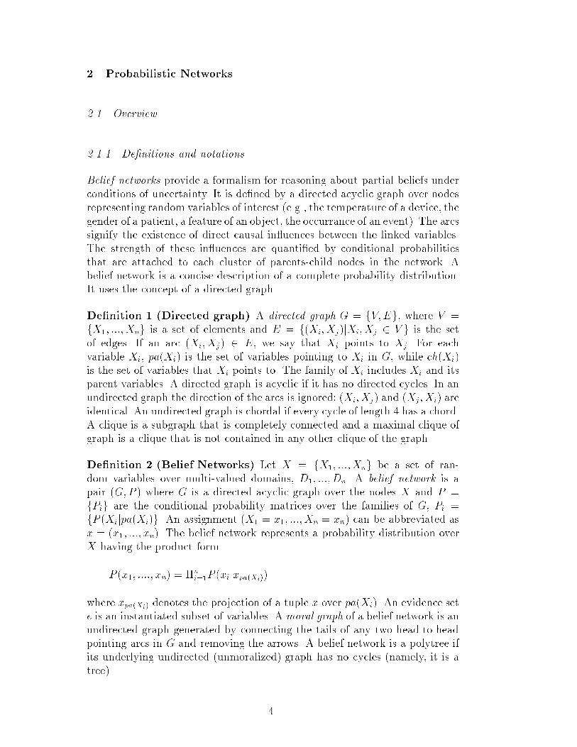
Fig. 1. (a) A belief network and (b) its moral graph
De�nition 3 (Induced width, induced graph) An ordered graph is a pair(G; d) where G is an undirected graph and d = X1; :::;Xn is an ordering ofthe nodes. The width of a node in an ordered graph is the number of itsearlier neighbors. The width w(d) of an ordering d, is the maximum widthover all nodes. The induced width of an ordered graph, w�(d), is the width ofthe induced ordered graph obtained by processing the nodes recursively, fromlast to �rst; when node X is processed, all its earlier neighbors are connected.This process is also called \triangulation". The induced (triangulated) graphis clearly chordal. The induced width of a graph, w�, is the minimal inducedwidth over all its orderings [10].
Example 4 Figure 1 shows a belief network's acyclic graph and its associatedmoral graph. The induced-width of the graph in Figure 1b along the orderingd = A;B;C;D;G;E;F;H is 3. Since the moral graph in Figure 1(b) is chordalno arc is added when generating the induced ordered graph. Therefore, theinduced-width w� of the graph is also 3.
Two of the most common tasks over belief networks are, to determine poste-rior beliefs and to �nd the most probable explanation (mpe), given a set ofobservations, or evidence. It is well known that such tasks can be answerede�ectively for singly-connected polytrees by a belief propagation algorithm[11]. This algorithm can be extended to multiply-connected networks by ei-ther tree-clustering or loop-cutset conditioning [11].
2.1.2 Tree-clustering
The most widely used method for processing belief networks is join-tree clus-tering. The algorithm transforms the original network into a tree of subprob-lems called join-tree. Tree-clustering methods have two parts. In the �rst partthe structure of the newly generated tree problem is decided, and in the secondpart the conditional probabilities between the subproblems, (viewed as high-dimensional variables) is determined. The structure of the join-tree is deter-
5
mined by graph information only, embedding the graph in a tree of cliques asfollows. First the moral graph is embedded in a chordal graph by adding someedges. This is accomplished by picking a variable ordering d = X1; :::;Xn,then, moving from Xn to X1, recursively, connecting all the earlier neighborsof Xi in the moral graph yielding the induced ordered graph. Its induced widthw�(d), as de�ned earlier, is the maximal number of earlier neighbors each nodehas.
Clearly, each node and its earlier neighbors in the induced graph is a clique.The maximal cliques, indexed by their latest variable in the ordering, can beconnected into a clique-tree and serve as the subproblems (or clusters) in the�nal join-tree. The clique-tree is created by connecting every clique Ci to anearlier clique Cj with whom it shares a maximal number of variables. Thisclique is called its parent clique. Clearly, the induced width w�(d) equals thesize of the maximal clique minus 1.
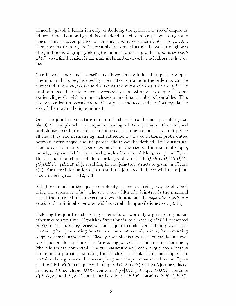
Once the join-tree structure is determined, each conditional probability ta-ble (CPT ) is placed in a clique containing all its arguments. The marginalprobability distributions for each clique can then be computed by multiplyingall the CPTs and normalizing, and subsequently the conditional probabilitiesbetween every clique and its parent clique can be derived. Tree-clustering,therefore, is time and space exponential in the size of the maximal clique,namely, exponential in the moral graph's induced-width (plus 1). In Figure1b, the maximal cliques of the chordal graph are f (A,B),(B,C,D),(B,D,G),(G,D,E,F), (H,G,F,E)g, resulting in the join-tree structure given in Figure3(a). For more information on structuring a join-tree, induced-width and join-tree clustering see [11,12,3,13].
A tighter bound on the space complexity of tree-clustering may be obtainedusing the separator width. The separator width of a join-tree is the maximalsize of the intersections between any two cliques, and the separator width of agraph is the minimal separator width over all the graph's join-trees [12,14].
Tailoring the join-tree clustering scheme to answer only a given query is an-other way to save time.AlgorithmDirectional tree clustering (DTC), presentedin Figure 2, is a query-based variant of join-tree clustering. It improves tree-clustering by 1) recording functions on separators only and 2) by restrictingto query-based answers only. Clearly, each of this modi�cation can be incorpo-rated independently. Once the structuring part of the join-tree is determined,(the cliques are connected in a tree-structure and each clique has a parentclique and a parent separator), then each CPT is placed in one clique thatcontains its arguments. For example, given the join-tree structure in Figure3a, the CPT P (BjA) is placed in clique AB, P (CjB) and P (DjC) are placedin clique BCD, clique BDG contains P (GjB;D), Clique GDEF containsP (EjD;F ) and P (F jG), and �nally, clique GEFH contains P (HjG;F;E).
6
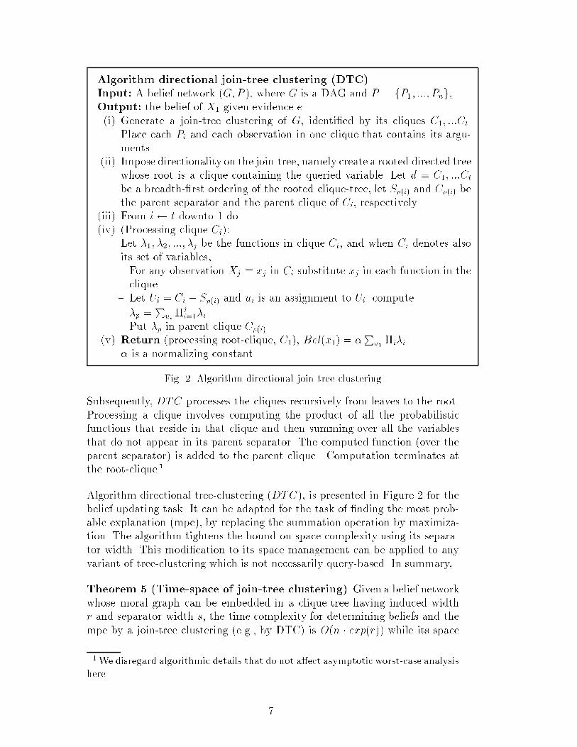
Algorithm directional join-tree clustering (DTC)Input: A belief network (G;P ), where G is a DAG and P = fP1; :::; Png,Output: the belief of X1 given evidence e.(i) Generate a join-tree clustering of G, identi�ed by its cliques C1; :::Ct.
Place each Pi and each observation in one clique that contains its argu-ments.
(ii) Impose directionality on the join-tree, namely create a rooted directed treewhose root is a clique containing the queried variable. Let d = C1; :::Ct
be a breadth-�rst ordering of the rooted clique-tree, let Sp(i) and Cp(i) bethe parent separator and the parent clique of Ci, respectively.
(iii) From i t downto 1 do(iv) (Processing clique Ci):
Let �1; �2; :::; �j be the functions in clique Ci, and when Ci denotes alsoits set of variables,{ For any observation Xj = xj in Ci substitute xj in each function in theclique.
{ Let Ui = Ci � Sp(i) and ui is an assignment to Ui. compute
�p =P
ui�ji=1�i.
Put �p in parent clique Cp(i).(v) Return (processing root-clique, C1), Bel(x1) = �
Pu1�i�i
� is a normalizing constant.
Fig. 2. Algorithm directional join-tree clustering
Subsequently, DTC processes the cliques recursively from leaves to the root.Processing a clique involves computing the product of all the probabilisticfunctions that reside in that clique and then summing over all the variablesthat do not appear in its parent separator. The computed function (over theparent separator) is added to the parent clique. Computation terminates atthe root-clique 1 .
Algorithm directional tree-clustering (DTC), is presented in Figure 2 for thebelief updating task. It can be adapted for the task of �nding the most prob-able explanation (mpe), by replacing the summation operation by maximiza-tion. The algorithm tightens the bound on space complexity using its separa-tor width. This modi�cation to its space management can be applied to anyvariant of tree-clustering which is not necessarily query-based. In summary,
Theorem 5 (Time-space of join-tree clustering) Given a belief networkwhose moral graph can be embedded in a clique-tree having induced widthr and separator width s, the time complexity for determining beliefs and thempe by a join-tree clustering (e.g., by DTC) is O(n � exp(r)) while its space
1We disregard algorithmic details that do not a�ect asymptotic worst-case analysishere.
7

complexity is O(n � exp(s)). 2
Clearly s � r. Note that since in the example of Figure1 the separator widthis 3 and the induced width is also 3, we do not gain much space-wise, bythe modi�ed algorithm. There are, however, many cases where the separatorwidth is much smaller than the induced-width.
2.1.3 Cycle-cutset conditioning
Belief networks may be processed also by cutset conditioning [11]. A subsetof nodes is called a cycle-cutset of an undirected graph if removing all theedges incident to nodes in the cutset makes the graph cycle-free. A subset ofnodes of an acyclic-directed graph is called a loop-cutset if removing all theoutgoing edges of nodes in the cutset results in a poly-tree [11,15]. A minimalcycle-cutset (resp. minimal loop-cutset) is such that if one node is removedfrom the set, the set is no longer a cycle-cutset (resp., a loop-cutset).
Algorithm cycle-cutset -conditioning (also called cycle-cutset decomposition orloop-cutset conditioning) is based on the observation that assigning a value toa variable changes the connectivity of the network. Graphically this amountsto removing all outgoing arcs from the assigned variables. Consequently, anassignment to a subset of variables that constitute a loop-cutset means thatbelief updating, conditioned on this assignment, can be carried out in theresulting poly-tree [11]. Multiply-connected belief networks can therefore beprocessed by enumerating all possible instantiations of a loop-cutset and solv-ing each conditioned network using the poly-tree algorithm. Subsequently, theconditioned beliefs are combined using a weighted sum where the weights arethe probabilities of the joint assignments to the loop-cutset variables condi-tioned on the evidence. Pearl [11] showed that weights computation is notmore costly than enumerating all the conditioned beliefs.
This scheme was later simpli�ed by Peot and Shachter [15]. They showedthat if the polytree algorithm is modi�ed to compute the probability of eachvariable-value proposition conjoined with the evidence, rather than conditionedon the evidence, the weighted sum can be replaced by a simple sum. In otherwords:
P (xje) = �P (x; e) = �X
c
P (x; e; c)
If fXg[C[E is a loop-cutset (note that C and E denote subsets of variables)then P (x; e; c) can be computed very e�ciently using a propagation-like algo-rithm on poly-trees. Consequently the complexity of the cycle-cutset scheme isexponential in the size of C where C [fXg[E is a loop-cutset. In summary,
Theorem 6 ([11,15]) Given a probabilistic network having a loop-cutset of
8

A B
B C D
B D G
G D E F
G E F H
B
B D
G D G E F
A B
B C D
B D G
B
B D
G D
A B
B C D G E F HG D E F H
B
(a) T0 (b) T1 (c) T2
Fig. 3. A tree-decomposition with separators equal to (a) 3, (b) 2, and (c) 1
size c, belief updating and mpe can be computed in time O(exp(c+ 2)) 2 andin linear space. 2
2.2 Trading Space for Time
Assume now that we have a problem whose join-tree has induced width r andseparator width s but space restrictions do not allow the necessary O(exp(s))memory required by tree-clustering. One way to overcome this problem is tocollapse cliques joined by large separators into one big cluster. The resultingjoin-tree has larger subproblems but smaller separators. This yields a sequenceof tree-decomposition algorithms parameterized by the sizes of their separa-tors.
De�nition 7 (Primary and secondary join-trees) Let T be a clique-treeembedding of the moral graph of G. Let s0; s1; :::; sn be the sizes of the sepa-rators in T listed in strictly descending order. With each separator size si, weassociate a tree decomposition Ti generated by combining adjacent clusterswhose separator sizes are strictly greater than si. T = T0 is called the primaryjoin-tree, while Ti, when i > 0, is a secondary join-tree. We denote by ri thelargest cluster size in Ti.
Note that as si decreases, ri increases. Clearly, from Theorem 1 it follows that
Theorem 8 Given a join-tree T , having separator sizes s0; s1; :::; st and cor-responding secondary join-trees having maximal clusters, r0; r1; :::; rt, beliefupdating and mpe can be computed using any one of the following time andspace bounds O(n � exp(ri)) time, and O(n � exp(si)) space, (i randing over allthe sequence of secondary join-trees), respectively.
2 the \2" in the exponent comes from the fact that belief updating on trees is linearin the size of the CPTs which are at least O(c2).
9
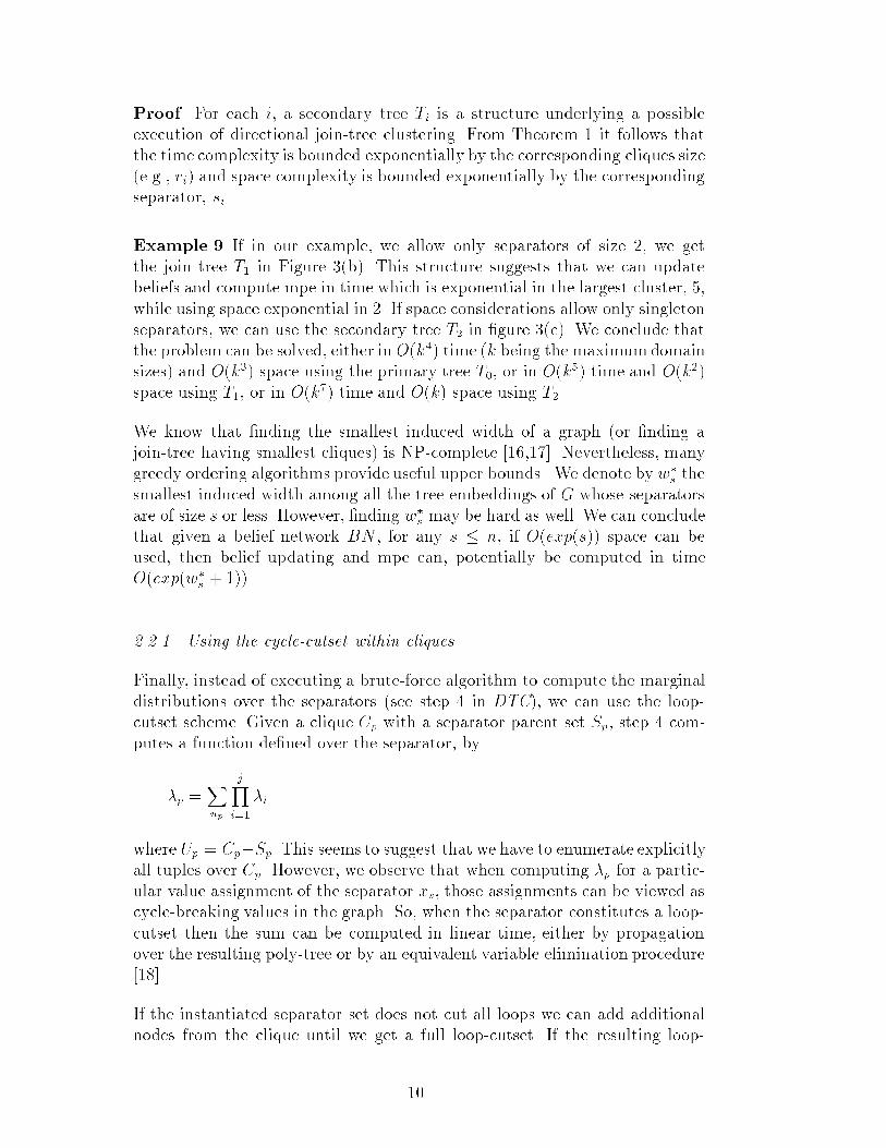
Proof. For each i, a secondary tree Ti is a structure underlying a possibleexecution of directional join-tree clustering. From Theorem 1 it follows thatthe time complexity is bounded exponentially by the corresponding cliques size(e.g., ri) and space complexity is bounded exponentially by the correspondingseparator, si.
Example 9 If in our example, we allow only separators of size 2, we getthe join tree T1 in Figure 3(b). This structure suggests that we can updatebeliefs and compute mpe in time which is exponential in the largest cluster, 5,while using space exponential in 2. If space considerations allow only singletonseparators, we can use the secondary tree T2 in �gure 3(c). We conclude thatthe problem can be solved, either in O(k4) time (k being the maximumdomainsizes) and O(k3) space using the primary tree T0, or in O(k5) time and O(k2)space using T1, or in O(k7) time and O(k) space using T2.
We know that �nding the smallest induced width of a graph (or �nding ajoin-tree having smallest cliques) is NP-complete [16,17]. Nevertheless, manygreedy ordering algorithms provide useful upper bounds. We denote by w�
s thesmallest induced width among all the tree embeddings of G whose separatorsare of size s or less. However, �nding w�
s may be hard as well. We can concludethat given a belief network BN , for any s � n, if O(exp(s)) space can beused, then belief updating and mpe can, potentially be computed in timeO(exp(w�
s + 1)).
2.2.1 Using the cycle-cutset within cliques
Finally, instead of executing a brute-force algorithm to compute the marginaldistributions over the separators (see step 4 in DTC), we can use the loop-cutset scheme. Given a clique Cp with a separator parent set Sp, step 4 com-putes a function de�ned over the separator, by
�p =X
up
jY
i=1
�i
where Up = Cp�Sp. This seems to suggest that we have to enumerate explicitlyall tuples over Cp. However, we observe that when computing �p for a partic-ular value assignment of the separator xs, those assignments can be viewed ascycle-breaking values in the graph. So, when the separator constitutes a loop-cutset then the sum can be computed in linear time, either by propagationover the resulting poly-tree or by an equivalent variable elimination procedure[18].
If the instantiated separator set does not cut all loops we can add additionalnodes from the clique until we get a full loop-cutset. If the resulting loop-
10
cutset (containing the separator variables) has size cs, clique's processing istime exponential in cs only and not in the full size of the clique.
In summary, given a join-tree decomposition, we can choose a loop-cutset of aclique Ci that is a minimal subset of variables, which together with its parentseparator-set that constitute a loop-cutset of the subnetwork de�ned over Ci.We conclude:
Theorem 10 Given a constant s � n, let Ts be a clique-tree whose separatorwidth has size s or less, and let c�s be the maximum size of a minimal cycle-cutset in any subgraph de�ned by the cliques in Ts. Then belief assessmentand mpe can be computed in space O(n � exp(s)) and in time O(n � exp(c�s)),and c�s � s, while c�s is smaller than the clique size.
Proof. Since computation in each clique is done by the cycle-cutset condi-tioning, its time is exponentially bounded by c�s, the maximal cycle-cutset overall the cliques of Ts, denoted c�s. The space complexity remains exponentialin the maximum separator s. Since for every clique, the loop-cutset we selectcontains its parent separator, then clearly c�s > s.
Next we give two examples. The �rst demonstrates the time-space tradeo�when using cycle-cutset in each clique. The second demonstrates in detailsthe mechanism of processing each clique by the cycle-cutset method.
Example 11 Considering the join-trees in Figure 3, if we apply the cycle-cutset scheme inside each subnetwork de�ned by each clique, we get no im-provement in the bound for T0 because the largest loop-cutset size in eachcluster is 3 since it always exceeds the largest separator. Remember also thatonce a loop-cutset is instantiated processing the simpli�ed network by prop-agation or by any e�cient method is also O(k2). However, when using thesecondary tree T1, we can reduce the time bound from O(k5) to O(k4) withonly O(exp(2)) space because the cutset size of the largest subgraph restrictedto fG;D;E;F;Hg, is 2; in this case the separator fC;Dg is already a loop-cutset and therefore when applying conditioning to this subnetwork the overalltime complexity is now O(k4). When applying conditioning to the clusters inT2, we get a time bound of O(k5) with just O(k) space because, the loop-cutsetof the subnetwork over fB;C;D;G;E;F;Hg has three nodes only fB;G;Eg.In summary, the dominating tradeo�s (when considering only the exponents)are between an algorithm based on T1 that requires O(k4) time and quadraticspace and an algorithm based on T2 that requires O(k5) time and O(k) space.
Example 12 We conclude this section by demonstrating through our exam-ple in Figure 1, the mechanics of processing a subnetwork by (1) a brute-forcemethods and (2) by loop-cutset conditioning. We will use join-tree T2 and
11
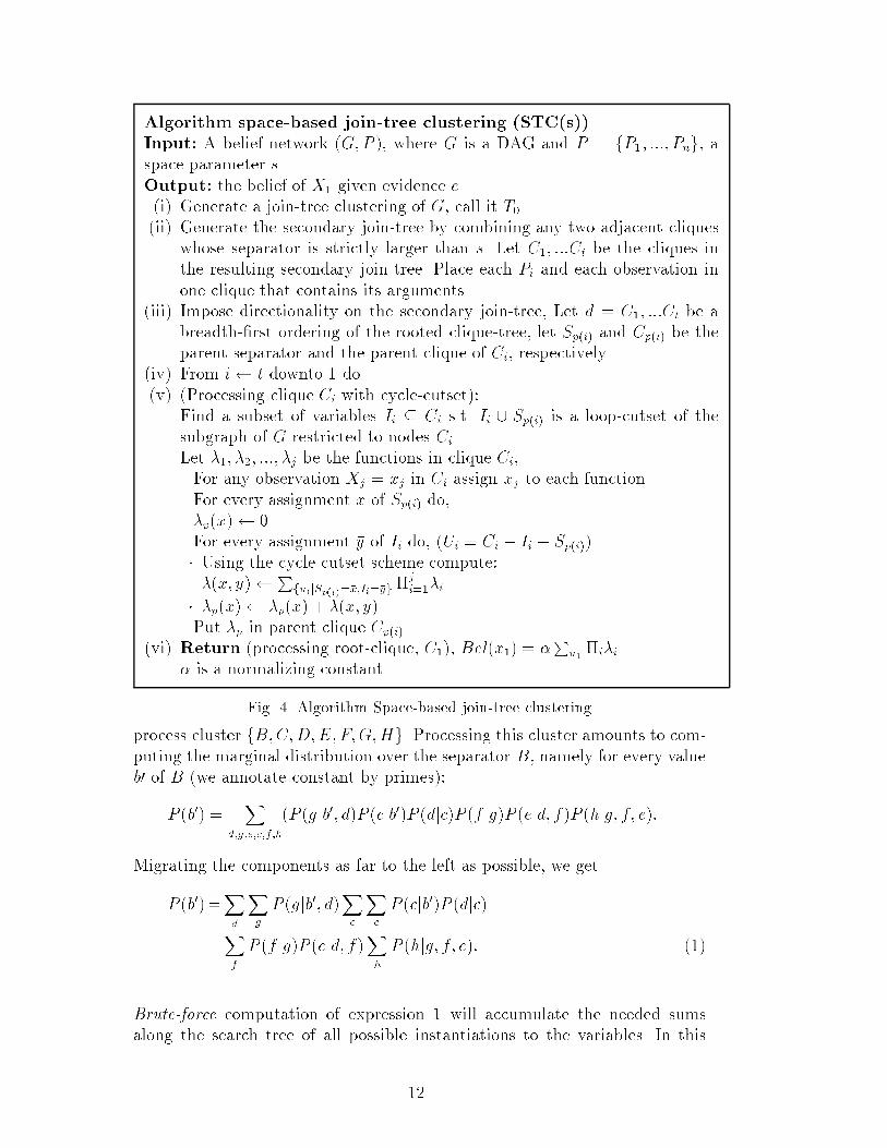
Algorithm space-based join-tree clustering (STC(s))Input: A belief network (G;P ), where G is a DAG and P = fP1; :::; Png, aspace parameter s.Output: the belief of X1 given evidence e.(i) Generate a join-tree clustering of G, call it T0.(ii) Generate the secondary join-tree by combining any two adjacent cliques
whose separator is strictly larger than s. Let C1; :::Ct be the cliques inthe resulting secondary join-tree. Place each Pi and each observation inone clique that contains its arguments.
(iii) Impose directionality on the secondary join-tree, Let d = C1; :::Ct be abreadth-�rst ordering of the rooted clique-tree, let Sp(i) and Cp(i) be theparent separator and the parent clique of Ci, respectively.
(iv) From i t downto 1 do(v) (Processing clique Ci with cycle-cutset):
Find a subset of variables Ii � Ci s.t. Ii [ Sp(i) is a loop-cutset of thesubgraph of G restricted to nodes Ci.Let �1; �2; :::; �j be the functions in clique Ci,{ For any observation Xj = xj in Ci assign xj to each function.{ For every assignment �x of Sp(i) do,�p(�x) 0.For every assignment �y of Ii do, (Ui = Ci � Ii � Sp(i))� Using the cycle-cutset scheme compute:�(�x; �y)
PfuijSp(i)=�x;Ii=�yg�
ji=1�i.
� �p(�x) �p(�x) + �(�x; �y)Put �p in parent clique Cp(i).
(vi) Return (processing root-clique, C1), Bel(x1) = �P
u1�i�i
� is a normalizing constant.
Fig. 4. Algorithm Space-based join-tree clustering
process cluster fB;C;D;E;F;G;Hg. Processing this cluster amounts to com-puting the marginal distribution over the separator B, namely for every valueb0 of B (we annotate constant by primes):
P (b0) =X
d;g;e;c;f;h
(P (gjb0; d)P (cjb0)P (djc)P (f jg)P (ejd; f)P (hjg; f; e):
Migrating the components as far to the left as possible, we get.
P (b0)=X
d
X
g
P (gjb0; d)X
e
X
c
P (cjb0)P (djc)
X
f
P (f jg)P (ejd; f)X
h
P (hjg; f; e): (1)
Brute-force computation of expression 1 will accumulate the needed sumsalong the search tree of all possible instantiations to the variables. In this
12
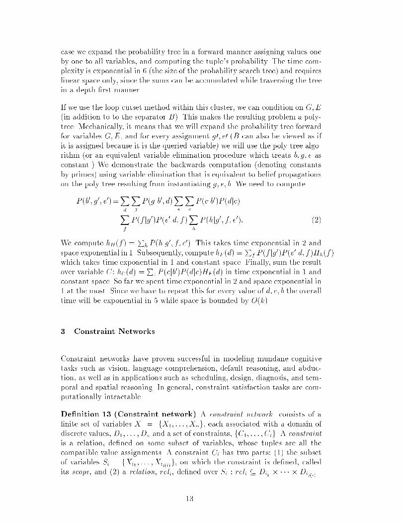
case we expand the probability tree in a forward manner assigning values oneby one to all variables, and computing the tuple's probability. The time com-plexity is exponential in 6 (the size of the probability search tree) and requireslinear space only, since the sums can be accumulated while traversing the treein a depth-�rst manner.
If we use the loop-cutset method within this cluster, we can condition on G;E(in addition to to the separator B). This makes the resulting problem a poly-tree. Mechanically, it means that we will expand the probability tree forwardfor variables G;E, and for every assignment g0; e0 (B can also be viewed as ifit is assigned because it is the queried variable) we will use the poly-tree algo-rithm (or an equivalent variable elimination procedure which treats b; g; e asconstant.) We demonstrate the backwards computation (denoting constantsby primes) using variable elimination that is equivalent to belief propagationson the poly-tree resulting from instantiating g; e; b. We need to compute
P (b0; g0; e0)=X
d
X
g
P (gjb0; d)X
e
X
c
P (cjb0)P (djc)
X
f
P (f jg0)P (e0jd; f)X
h
P (hjg0; f; e0): (2)
We compute hH(f) =P
h P (hjg0; f; e0). This takes time exponential in 2 and
space exponential in 1. Subsequently, compute hF (d) =P
f P (f jg0)P (e0jd; f)Hh(f)
which takes time exponential in 1 and constant space. Finally, sum the resultover variable C: hC(d) =
Pc P (cjb
0)P (djc)HF (d) in time exponential in 1 andconstant space. So far we spent time exponential in 2 and space exponential in1 at the most. Since we have to repeat this for every value of d; e; b the overalltime will be exponential in 5 while space is bounded by O(k).
3 Constraint Networks
Constraint networks have proven successful in modeling mundane cognitivetasks such as vision, language comprehension, default reasoning, and abduc-tion, as well as in applications such as scheduling, design, diagnosis, and tem-poral and spatial reasoning. In general, constraint satisfaction tasks are com-putationally intractable.
De�nition 13 (Constraint network) A constraint network consists of a�nite set of variables X = fX1; : : : ;Xng, each associated with a domain ofdiscrete values, D1; : : : ;Dn and a set of constraints, fC1; : : : ; Ctg. A constraintis a relation, de�ned on some subset of variables, whose tuples are all thecompatible value assignments. A constraint Ci has two parts: (1) the subsetof variables Si = fXi1 ; : : : ;Xij(i)g, on which the constraint is de�ned, calledits scope, and (2) a relation, reli, de�ned over Si : reli � Di1 � � � � � Dij(i) .
13

A
B
CD E
FG
H
B C D E F F H
E HA B
D G
G D FC D
B D
G HBG
D D
BB B
CD D
D
D G D FF
H
H
F
H
E
GB
BG G
Fig. 5. Primal (a) and dual (b) constraint graphs
The scheme of a constraint network is the set of scopes on which constraintsare de�ned. An assignment of a unique domain value to each member ofsome subset of variables is called an instantiation. A consistent instantiationof all the variables that does not violate any constraint is called a solution.Typical queries associated with constraint networks are to determine whethera solution exists and to �nd one or all solutions.
De�nition 14 (Constraint graphs) Two graphical representations of a con-straint network are its primal constraint graph and its dual constraint graph.A primal constraint graph represents variables by nodes and associates an arcwith any two nodes residing in the same constraint. A dual constraint graphrepresents each constraint subset by a node and associates a labeled arc withany two nodes whose constraint subsets share variables. The arcs are labeledby the shared variables.
Example 15 Figure 5 depicts the primal and the dual representations of anetwork having variables A; B; C; D; E; F; G;H whose constraints arede�ned on the subsets f(A;B); (B;C); (B;D), (C;D); (D;G); (G;E); (B;G),(D;E;F ); (G;D;F ); (G;H); (E;H)(F;H)g.
Tree clustering for constraint networks is similar to join-tree clustering forprobabilistic networks. In fact, the structuring part is identical. Once thejoin-tree structure is determined, each constraint is placed in a clique (or acluster) that contains its scope and then each clustered subproblem can besolved independently. In other words, the set of constraints in a clique can bereplaced by its set of solutions; a new constraint whose scope is the clique'svariables. The time and space complexity of tree-clustering is governed by thetime and space required to generate the relations of each clique in the join-tree which is exponential in the clique's size, and therefore in the problem'sinduced width w� [12,3].
Example 16 Since the graph in Figure 5(a) is identical to the graph in Fig-ure 1(b), it possesses the same clique-tree embeddings. Namely, the maximalcliques of the chordal graph are f(A;B); (B;C;D); (B;D;G);(G;D;E;F ); (H;G;F;E)g and a join-tree is given in Figure 3(a). The schemesof each clique's subproblem are:CAB = f(A;B)g, CBCD = f(B;C); (C;D)g,
14
CBDG = f(B;D); (B;G); (G;D)g,CGDEF = f(G;D); (D;E); (E;F ); (G;F ); (D;F )gCGEFH = f(E;F ); (G;F ); (G;H); (F;H); (E;H)g.As in the probabilistic case, a brute-force application of tree-clustering to thisproblem is time and space exponential in 4.
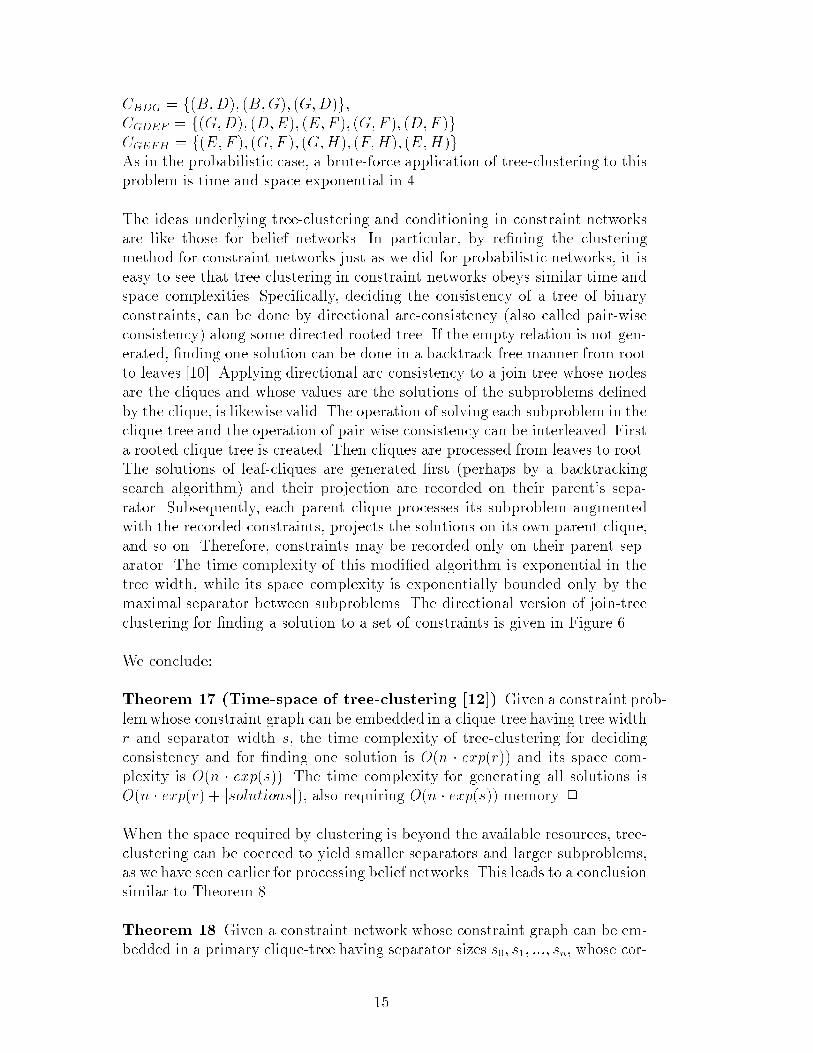
The ideas underlying tree-clustering and conditioning in constraint networksare like those for belief networks. In particular, by re�ning the clusteringmethod for constraint networks just as we did for probabilistic networks, it iseasy to see that tree-clustering in constraint networks obeys similar time andspace complexities. Speci�cally, deciding the consistency of a tree of binaryconstraints, can be done by directional arc-consistency (also called pair-wiseconsistency) along some directed rooted tree. If the empty relation is not gen-erated, �nding one solution can be done in a backtrack-free manner from rootto leaves [10]. Applying directional arc-consistency to a join-tree whose nodesare the cliques and whose values are the solutions of the subproblems de�nedby the clique, is likewise valid. The operation of solving each subproblem in theclique-tree and the operation of pair-wise consistency can be interleaved. Firsta rooted clique-tree is created. Then cliques are processed from leaves to root.The solutions of leaf-cliques are generated �rst (perhaps by a backtrackingsearch algorithm) and their projection are recorded on their parent's sepa-rator. Subsequently, each parent clique processes its subproblem augmentedwith the recorded constraints, projects the solutions on its own parent clique,and so on. Therefore, constraints may be recorded only on their parent sep-arator. The time complexity of this modi�ed algorithm is exponential in thetree width, while its space complexity is exponentially bounded only by themaximal separator between subproblems. The directional version of join-treeclustering for �nding a solution to a set of constraints is given in Figure 6.
We conclude:
Theorem 17 (Time-space of tree-clustering [12]) Given a constraint prob-lemwhose constraint graph can be embedded in a clique-tree having tree widthr and separator width s, the time complexity of tree-clustering for decidingconsistency and for �nding one solution is O(n � exp(r)) and its space com-plexity is O(n � exp(s)). The time complexity for generating all solutions isO(n � exp(r) + jsolutionsj), also requiring O(n � exp(s)) memory. 2
When the space required by clustering is beyond the available resources, tree-clustering can be coerced to yield smaller separators and larger subproblems,as we have seen earlier for processing belief networks. This leads to a conclusionsimilar to Theorem 8.
Theorem 18 Given a constraint network whose constraint graph can be em-bedded in a primary clique-tree having separator sizes s0; s1; :::; sn, whose cor-
15

Algorithm directional tree-clustering for CSPsInput: A set of constraints R1; :::; Rl over X = fX1; :::;Xng, having scopesS1; :::; Sl respectively, and its constraint graph G.Output: A solution to the constraint problem.(i) Generate a join-tree clustering of G, identi�ed by its cliques C1; :::Ct.
Place each Ri in one clique that contains its scope.(ii) Impose directionality on the join-tree, namely create a rooted directed tree
whose root is any clique . Let d = C1; :::Cl be a breadth-�rst ordering ofthe rooted clique-tree, let Sp(i) and Cp(i) be the parent separator and theparent clique of Ci, respectively.
(iii) From i downto 1 do(iv) (Processing clique Ci):
Let R1; R2; :::; Rj be the constraints in clique Ci, let Ui be the set ofvariables in clique Ci.{ Solve the subproblem in Ci and call the set of solutions �i. Projectthis set of solutions on the parent separator. Let �Sp(i) be the projected
relation. �Sp(i) QSp(i)
1jk=1 Rk
Put �Sp(i) in parent clique Cp(i).(v) Return generate a solution in a backtrack-free manner going from the
root clique towards the leaves.
Fig. 6. Algorithm directional join-tree clustering for constraints
responding maximal clique sizes in the secondary join-trees are r0; r1; :::; rn,then deciding consistency and �nding a solution can be accomplished using anyone of the time and space complexity bounds O(n �exp(ri)) and O(n �exp(si)),respectively.
Proof. Analogous to Theorem 3. 2
Similarly to belief networks, any linear-space method can replace backtrackingfor solving each of the subproblems de�ned by the cliques. One possibility is touse the cycle-cutset scheme. The cycle-cutset method for constraint networks(like in belief networks) enumerates the possible solutions to a set of cycle-cutset variables and, for each consistent cutset assignment, solves the restrictedtree-like problem in polynomial time. Thus, the overall time complexity is ex-ponential in the size of the cycle-cutset of the graph [19]. More precisely, it canbe shown that the cycle-cutset method is bounded by O(n � kc+2), where c isthe cutset size, k is the domain size, and n is the number of variables [19]. For-tunately, enumerating all the cycle-cutsets assignments can be accomplished
16

in linear space using a backtracking algorithm.
Theorem 19 Let G be a constraint graph and let T be a join-tree withseparator size s or less. Let cs be the largest minimal cycle-cutset 3 in anysubproblem in T . Then the problem can be solved in space O(n � exp(s)) andin time O(n � exp(cs + 2)), where cs � s.
Proof. Since the maximum separator size is s, then, from Theorem 17, tree-clustering requires O(n � exp(s)) space. Since the cycle-cutset's size in eachcluster is bounded by cs, the time complexity is exponentially bounded by cs.
Example 20 Applying the cycle-cutsetmethod to each subproblem in T0; T1; T2shows (see Figure 3), as before, that the best alternatives are an algorithm hav-ing O(k4) time and quadratic space, (using T1, since fG;Eg is a cycle-cutsetof the subgraph restricted to fG;D;E;F;Hg having size 2), and an algorithmhaving O(k5) time and O(k) space only (using T2, since the cycle-cutset sizeof the whole problem is 3).
A special case of Theorem 3, observed before in [10,20], is that when the graphis decomposed into non-separable components (i.e., when the separator sizeequals 1).
Corollary 21 If G has a decomposition to non-separable components suchthat the size of the maximal cutsets in each component is bounded by c, thenthe problem can be solved in O(n � exp(c)) time, using linear space. 2
4 Optimization Tasks
Clustering and conditioning are applicable also to optimization tasks de�nedover probabilistic and deterministic networks. An optimization task is de-�ned relative to a real-valued criterion or cost function associated with ev-ery instantiation. In the context of constraint networks, the task is to �nda consistent instantiation having maximum cost. Applications include diag-nosis and scheduling problems. In the context of probabilistic networks, thecriterion function denotes a utility or a value function, and the task is to �ndan assignment to a subset of decision variables that maximize the expectedcriterion function. Applications include planning and decision making underuncertainty. If the criterion function is decomposable, its structure can be
3As before, the cycle-cutset contains the separator set
17
augmented onto the corresponding graph (constraint graph or moral graph)to subsequently be exploited by either tree-clustering or conditioning.
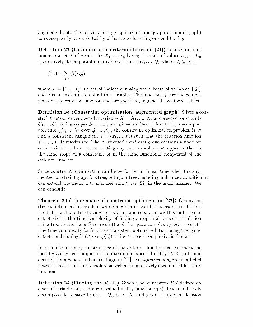
De�nition 22 (Decomposable criterion function [21]) A criterion func-tion over a set X of n variables X1; :::;Xn having domains of values D1; :::;Dn
is additively decomposable relative to a scheme Q1; :::; Qt where Qi � X i�
f(x) =X
i2T
fi(xQi);
where T = f1; :::; tg is a set of indices denoting the subsets of variables fQigand x is an instantiation of all the variables. The functions fi are the compo-nents of the criterion function and are speci�ed, in general, by stored tables.
De�nition 23 (Constraint optimization, augmented graph) Given a con-straint network over a set of n variablesX = X1; ::::;Xn and a set of constraintsC1; :::; Ct having scopes S1; :::; St, and given a criterion function f decompos-able into ff1; :::; flg over Q1; :::; Ql, the constraint optimization problem is to�nd a consistent assignment x = (x1; :::; xn) such that the criterion functionf =P
i fi, is maximized. The augmented constraint graph contains a node foreach variable and an arc connecting any two variables that appear either inthe same scope of a constraint or in the same functional component of thecriterion function.
Since constraint optimization can be performed in linear time when the aug-mented constraint graph is a tree, both join-tree clustering and cutset-conditioningcan extend the method to non-tree structures [22] in the usual manner. Wecan conclude:
Theorem 24 (Time-space of constraint optimization [22]) Given a con-straint optimization problem whose augmented constraint graph can be em-bedded in a clique-tree having tree width r and separator width s and a cycle-cutset size c, the time complexity of �nding an optimal consistent solutionusing tree-clustering is O(n � exp(r)) and the space complexity O(n � exp(s)).The time complexity for �nding a consistent optimal solution using the cycle-cutset conditioning is O(n � exp(c)) while its space complexity is linear. 2
In a similar manner, the structure of the criterion function can augment themoral graph when computing the maximum expected utility (MEU) of somedecisions in a general in uence diagram [23]. An in uence diagram is a beliefnetwork having decision variables as well as an additively decomposable utilityfunction.
De�nition 25 (Finding the MEU) Given a belief network BN de�ned ona set of variables X, and a real-valued utility function u(x) that is additivelydecomposable relative to Q1; :::; Qt, Qi � X, and given a subset of decision
18

variables D = fD1; :::Dkg that are root variables in the directed acyclic graphof the BN , the MEU task is to �nd an assignment �dok = (do1; :::; dok) such that
( �dok) = argmax �dk
X
xk+1;:::;xn
�ki=1P (xijxpa(Xi);
�dk)u(x):
The utility-augmented graph of an in uence diagram is its moral graph withsome additional edges: any two nodes appearing in the same component ofthe utility function are connected as well.
A linear-time propagation algorithm can compute the MEU whenever theutility-augmented moral graph of the network is a tree [24]. Consequently, byexploiting the augmented moral graph, we can extend this propagation al-gorithm to general in uence diagrams. The two approaches that extend thispropagation algorithm to multiply-connected networks, cycle-cutset condition-ing and join-tree clustering, are applicable here as well [11,13,23]. It was alsoshown that elimination algorithms are similar to tree-clustering methods [12].In summary:
Theorem 26 (Time-space of �nding the MEU) Given a belief networkhaving a subset of decision variables, and given an additively decomposableutility function whose augmented moral graph can be embedded in a clique-tree having tree width r and separator width s and a cycle-cutset size c,the time complexity of computing the MEU using tree-clustering is O(n �exp(r)) and the space complexity is O(n � exp(s)). The time complexity for�nding aMEU using cycle-cutset conditioning is O(n �exp(c)) while the spacecomplexity is linear. 2
Once we have established the graph that guides tree-clustering and condi-tioning for either constraint optimization or for �nding the MEU, the sameprinciple of trading space for time becomes applicable and will yield a col-lection of parametrized algorithms governed by the primary and secondaryclique-trees and cycle-cutsets of the augmented graphs as we have seen before.
The following theorem summarizes the time and space tradeo�s associatedwith optimization tasks.
Theorem 27 Given a constraint network (resp., a belief network) and givenan additively decomposable criterion function f , if the augmented constraintgraph (resp., moral graph) relative to the criterion function can be embeddedin a clique-tree having separator sizes s0; s1; :::sn, and corresponding maxi-mal clique sizes r0; r1; :::; rn and corresponding maximal minimal cutset sizesc0; c1; :::; cn, then �nding an optimal solution (resp., �nding the maximum ex-pected criterion value) can be accomplished using any one of the followingbounds on the time and space: if a brute-force approach is used for processingeach subproblem the bounds are O(n�exp(ri)) time and O(n�exp(si)) space. If
19
C
A
B
D E
G F
H
G D E F
B G D G E F H
C D BA B G
B G
G D
B D
G E F
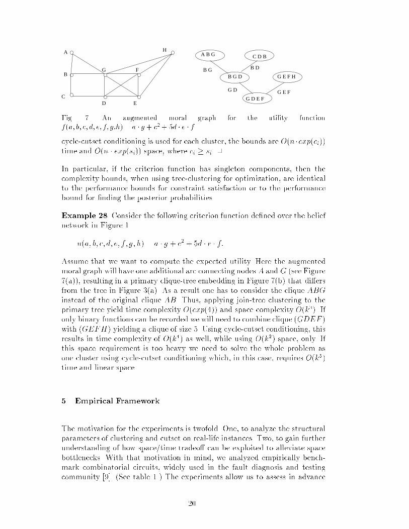
Fig. 7. An augmented moral graph for the utility functionf(a; b; c; d; e; f; g:h) = a � g + c2 + 5d � e � f
cycle-cutset conditioning is used for each cluster, the bounds are O(n �exp(ci))time and O(n � exp(si)) space, where ci � si. 2
In particular, if the criterion function has singleton components, then thecomplexity bounds, when using tree-clustering for optimization, are identicalto the performance bounds for constraint satisfaction or to the performancebound for �nding the posterior probabilities.
Example 28 Consider the following criterion function de�ned over the beliefnetwork in Figure 1
u(a; b; c; d; e; f; g; h) = a � g + c2 + 5d � e � f:
Assume that we want to compute the expected utility. Here the augmentedmoral graph will have one additional arc connecting nodes A and G (see Figure7(a)), resulting in a primary clique-tree embedding in Figure 7(b) that di�ersfrom the tree in Figure 3(a). As a result one has to consider the clique ABGinstead of the original clique AB. Thus, applying join-tree clustering to theprimary tree yield time complexity O(exp(4)) and space complexity O(k3). Ifonly binary functions can be recorded we will need to combine clique (GDEF )with (GEFH) yielding a clique of size 5. Using cycle-cutset conditioning, thisresults in time complexity of O(k4) as well, while using O(k2) space, only. Ifthis space requirement is too heavy we need to solve the whole problem asone cluster using cycle-cutset conditioning which, in this case, requires O(k5)time and linear space.
5 Empirical Framework
The motivation for the experiments is twofold. One, to analyze the structuralparameters of clustering and cutset on real-life instances. Two, to gain furtherunderstanding of how space/time tradeo� can be exploited to alleviate spacebottlenecks. With that motivation in mind, we analyzed empirically bench-mark combinatorial circuits, widely used in the fault diagnosis and testingcommunity [9]. (See table 1.) The experiments allow us to assess in advance
20
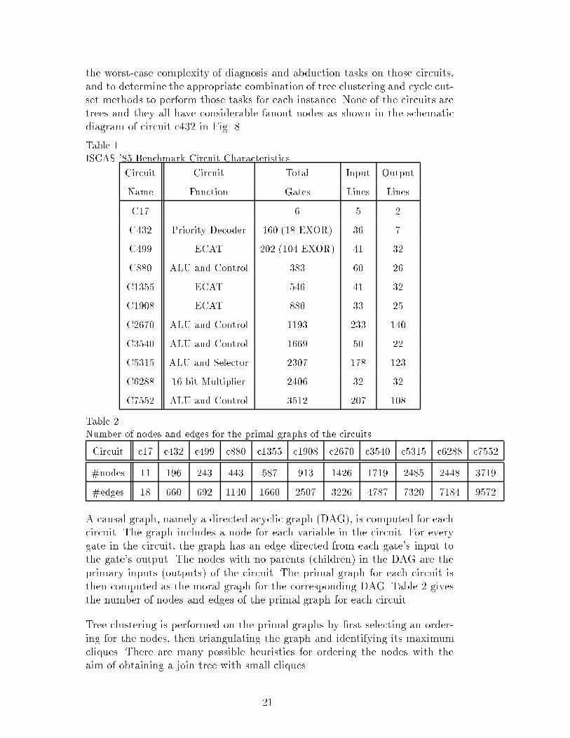
the worst-case complexity of diagnosis and abduction tasks on those circuits,and to determine the appropriate combination of tree clustering and cycle cut-set methods to perform those tasks for each instance. None of the circuits aretrees and they all have considerable fanout nodes as shown in the schematicdiagram of circuit c432 in Fig. 8.
Table 1ISCAS '85 Benchmark Circuit Characteristics
Circuit Circuit Total Input Output
Name Function Gates Lines Lines
C17 6 5 2
C432 Priority Decoder 160 (18 EXOR) 36 7
C499 ECAT 202 (104 EXOR) 41 32
C880 ALU and Control 383 60 26
C1355 ECAT 546 41 32
C1908 ECAT 880 33 25
C2670 ALU and Control 1193 233 140
C3540 ALU and Control 1669 50 22
C5315 ALU and Selector 2307 178 123
C6288 16-bit Multiplier 2406 32 32
C7552 ALU and Control 3512 207 108
Table 2Number of nodes and edges for the primal graphs of the circuits.
Circuit c17 c432 c499 c880 c1355 c1908 c2670 c3540 c5315 c6288 c7552
#nodes 11 196 243 443 587 913 1426 1719 2485 2448 3719
#edges 18 660 692 1140 1660 2507 3226 4787 7320 7184 9572
A causal graph, namely a directed acyclic graph (DAG), is computed for eachcircuit. The graph includes a node for each variable in the circuit. For everygate in the circuit, the graph has an edge directed from each gate's input tothe gate's output. The nodes with no parents (children) in the DAG are theprimary inputs (outputs) of the circuit. The primal graph for each circuit isthen computed as the moral graph for the corresponding DAG. Table 2 givesthe number of nodes and edges of the primal graph for each circuit.
Tree clustering is performed on the primal graphs by �rst selecting an order-ing for the nodes, then triangulating the graph and identifying its maximumcliques. There are many possible heuristics for ordering the nodes with theaim of obtaining a join tree with small cliques.
21
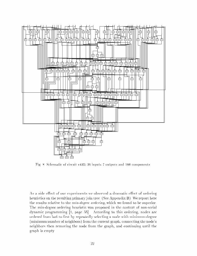
Fig. 8. Schematic of circuit c432: 36 inputs 7 outputs and 160 components.
As a side e�ect of our experiments we observed a dramatic e�ect of orderingheuristics on the resulting primary join tree. (See Appendix B). We report herethe results relative to the min-degree ordering, which we found to be superior.The min-degree ordering heuristic was proposed in the context of non-serialdynamic programming [4, page 55]. According to this ordering, nodes areordered from last to �rst by repeatedly selecting a node with minimumdegree(minimumnumber of neighbors) from the current graph, connecting the node'sneighbors then removing the node from the graph, and continuing until thegraph is empty.
22
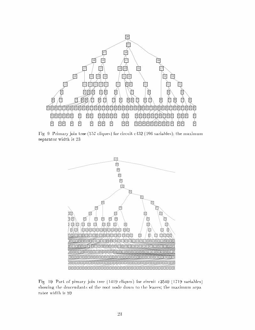
Fig. 9. Primary join tree (157 cliques) for circuit c432 (196 variables); the maximumseparator width is 23.
Fig. 10. Part of pimary join tree (1419 cliques) for circuit c3540 (1719 variables)showing the descendants of the root node down to the leaves; the maximum sepa-rator width is 89.
23

6 Empirical Results
6.1 Pure Clustering; Primary Join Trees
For each primary join tree generated, three parameters are computed: (1) thesize of cliques, (2) the size of cycle-cutsets in each of the subgraphs de�nedby the cliques, and (3) the size of the separator sets. The nodes of the jointree are labeled by the cliques (or clusters) sizes and the edges are labeledby the separator width. In this section we present the results on two circuitsc432 and c3540, having 196 and 1719 variables, respectively. Results on othercircuits are summarized in Appendix A and C.
Figure 9 and 10 present information on the primary join trees. Figure 9 showsthat the cliques sizes range from 2 to 28. The root node has 28 nodes and thedescendant nodes have strictly smaller sizes. The depth of the tree is 11 andall nodes whose distance from the root is greater than 6 have sizes stricly lessthan 10. The leaves have sizes ranging from 2 to 6. Similar observations canbe made for the primary join tree of the larger circuit c3540 shown in Fig. 10.
Frequencies
Cliq
ue s
ize
10 20 30 40
Clique sizes for c432Total number= 157,Maximum= 28Mode= 5,Median= 6,Mean= 7.43312
234567891011121719212728
Frequencies
Sep
arat
or w
idth
10 20 30 40
Separator widths for c432Total number= 156,Maximum= 23Mode= 4,Median= 5,Mean= 6.22436
1
2
3
4
5
6
7
8
9
10
11
16
18
20
23
Frequencies
Cut
set s
ize
20 40 60 80
Cutset sizes for c432Total number= 157,Maximum= 17Mode= 1,Median= 1,Mean= 1.92357
0
1
2
3
4
5
7
8
9
10
16
17
Fig. 11. Histograms of the cliques sizes, the separator widths and the cutsets sizesof the primary join tree for circuit c432 (196 variables)
Figures 11 and 12 provide additional details showing the frequencies of cliquessizes, separator widths and cutsets sizes for both circuits. Those �gures (and allthe corresponding �gures in Appendix A) show that the structural parametersare skewed with the vast majority of the parameters having values below themidpoint (the point dividing the range of values from smallest to largest).
We see in Figure 11 that the number of cliques is 157 and the cliques sizesare in the range from 2 to 28. The mode is 5, the median is 6 and the meanis 7.433. 40 cliques out of the total 157 have size 5, and only 23 out of 157have size greater than 9. The separator widths are in the range from 1 to 23.The mode is 4, the median is 5 and the mean is 6.224. Out of the total 156separator widths, 40 have size 4 and only 13 have sizes greater than 10. The
24
Frequencies
Cliq
ue s
ize
100 200 300 400
Clique sizes for c3540Total number= 1419,Maximum= 114Mode= 4,Median= 5,Mean= 8.15645
2
3
4
5
6
7
8
9
10
11
12
13
14
Frequencies
Sep
arat
or w
idth
100 200 300 400 500
Separator widths for c3540Total number= 1418,Maximum= 89Mode= 3,Median= 4,Mean= 6.94993
1
2
3
4
5
6
7
8
9
10
11
12
13
Frequencies
Cut
set s
ize
100 200 300 400 500 600 700
Cutset sizes for c3540Total number= 1419,Maximum= 16Mode= 1,Median= 1,Mean= 1.32488
0
1
2
3
4
5
6
7
9
10
11
13
16
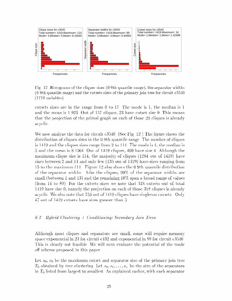
Fig. 12. Histograms of the cliques sizes (0.9th quantile range), the separator widths(0.9th quantile range) and the cutsets sizes of the primary join tree for circuit c3540(1719 variables).
cutsets sizes are in the range from 0 to 17. The mode is 1, the median is 1and the mean is 1.923. Out of 157 cliques, 23 have cutset size 0. This meansthat the projection of the primal graph on each of those 23 cliques is alreadyacyclic.
We now analyze the data for circuit c3540. (See Fig. 12.) The �gure shows thedistribution of cliques sizes in the 0.9th quantile range. The number of cliquesis 1419 and the cliques sizes range from 2 to 114. The mode is 4, the median is5 and the mean is 8.1564. Out of 1419 cliques, 400 have size 4. Although themaximum clique size is 114, the majority of cliques (1284 out of 1419) havesizes between 2 and 14 and only few (135 out of 1419) have sizes ranging from15 to the maximum 114. Figure 12 also shows the 0.9th quantile distributionof the separator widths. Like the cliques, 90% of the separator widths aresmall (between 1 and 13) and the remaining 10% span a broad range of values(from 14 to 89). For the cutsets sizes we note that 318 cutsets out of total1419 have size 0, namely the projection on each of those 318 cliques is alreadyacyclic. We also note that 753 out of 1419 cliques have singleton cutsets. Only47 out of 1419 cutsets have sizes greater than 5.
6.2 Hybrid Clustering + Conditioning; Secondary Join Trees
Although most cliques and separators are small, some will require memoryspace exponential in 23 for circuit c432 and exponential in 89 for circuit c3540.This is clearly not feasible. We will next evaluate the potential of the tradeo� scheme proposed in this paper.
Let s0, c0 be the maximum cutset and separator size of the primary join treeT0 obtained by tree clustering. Let s0; s1; : : : ; sn be the size of the separatorsin T0 listed from largest to smallest. As explained earlier, with each separator
25

size, si, we associate a tree decomposition Ti generated by combining adjacentclusters whose separators' sizes are strictly larger than si. We denote by ci thelargest cutset size in any cluster of Ti.
We estimate the space/time bounds for each circuit based on the graph pa-rameters observed using our tree decomposition scheme. Figure 13 gives achart providing bounds for time versus space for each circuit. Each point inthe chart corrseponds to a speci�c secondary join tree decomposition Ti andhas the space complexity measured by the separator width, si, and the timecomplexity by the maximum between the separator width and the cutset size;max(si; ci). Each chart in Figure 13 can be used to select the algorithm fromthe spectrum of conditioning+clustering algorithms of our tree decompositionscheme that best meets a given time-space speci�cation. Each chart showsthe gradual e�ect of lowering the available space on the time required bya corresponding clustering+conditioning algorithm. For example circuit c432(Figure 13) shows the separator width (space) which is initially 23 (for the pri-mary join tree) gradually reduced down to 1 in a series of secondary trees. The�gure shows that reducing the separator width to meet the space available fora conditioning+clustering algorithm increases the worst-case time complexityof the algorithm. The time complexity increases becasue of the larger clusterscontained in the secondary join tree and the increase in the size of the cutsetfor those clusters. It is interesting to note that the charts in Figure 13 alldisplay a \knee" phenomenon in the time-space tradeo� where time increasesonly slightly for a broad range of space reduction beyond which further re-duction in space causes signi�cant rise in the time bound. We also note thatthe time estimate shown in Figure 13 displays a small dip before it rises withthe decrease in available space. For example for circuit c432 we note a dipwhen the space is decreased from 23 to 20. This can be explained as follows.As mentioned earlier we measure the worst-case time complexity as the max-imum between the separator width and the cutset size. This is so since timecomplexity always exceeds space complexity. As the space measured by theseparator width decreases the secondary join trees will contain larger clustersand their cutset size will also increase. However, the rate of increase of thecutset sizes does not grow linearly with the decrease in the separator width.The results shown in Figure 13 indicate that for small decrease in separatorwidth (space) the cutset size will increase by an amount smaller than theamount of decrease in the separator width. This explains the dip in the timecomplexity. However, beyond that dip further decrease in the separator width(space) will cause an increase in the cutset size that dominates the decrease inthe separator width and the rate of time increase becomes staggering as thealgorithms approach the lowest bound of linear space.
Figures 14-16 display the structure of the join trees for c432 for separatorwidths ranging from 23 down to 3. As the separator decreases the maximumclique size increases, and both the size and the depth of the tree decrease. Like
26

10 20 30 40
Space
50100150200250300
Time
Circuit c1908
0 5 10 15 20 25 30
Space
100
200
300
400
Time
Circuit c2670
0 5 10 15 20
Space
20406080
100120140160
Time
Circuit c880
2.5 5 7.5 1012.51517.5
Space
50
100
150
200
Time
Circuit c1355
5 10 15 20
Space
20304050607080
Time
Circuit c432
2.5 5 7.5 1012.51517.5
Space
203040506070
Time
Circuit c499
Fig. 13. Time/Space tradeo� for c432 (196 variables), c499 (243 variables), c880 (443variables), c1355 (587 variables), c1908 (913 variables) and c2670 (1426 variables).Time is measured by the maximum of the separator width and the cutset size andspace by the maximum separator width.
the primary join tree, each secondary join tree has also a skewed distributionof the clique sizes. Note that the clique size for the root node is signi�cantlylarger than for all other nodes, and is increasing as the separator decreases.For instance, the root node for the secondary join tree with separator width 20(Figure 14) has size 32 while all other nodes have sizes in the range from 2 to
27

21. When reducing the separator width to 3 the secondary join tree (Figure 16)has the root node with size 172 while all other nodes have sizes in the rangefrom 2 to 4.
Fig. 14. Secondary trees for c432 with separator widths 23 and 20
28
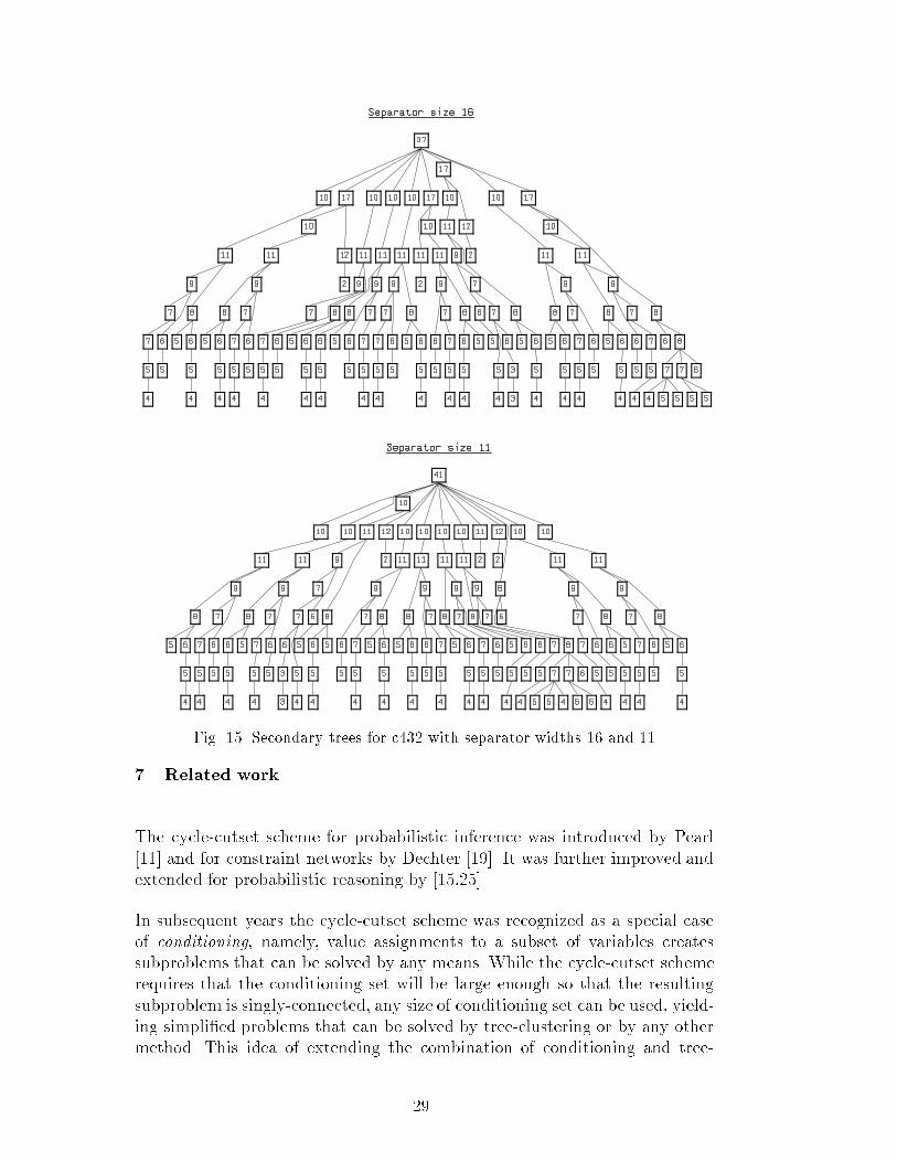
Fig. 15. Secondary trees for c432 with separator widths 16 and 11
7 Related work
The cycle-cutset scheme for probabilistic inference was introduced by Pearl[11] and for constraint networks by Dechter [19]. It was further improved andextended for probabilistic reasoning by [15,25].
In subsequent years the cycle-cutset scheme was recognized as a special caseof conditioning, namely, value assignments to a subset of variables createssubproblems that can be solved by any means. While the cycle-cutset schemerequires that the conditioning set will be large enough so that the resultingsubproblem is singly-connected, any size of conditioning set can be used, yield-ing simpli�ed problems that can be solved by tree-clustering or by any othermethod. This idea of extending the combination of conditioning and tree-
29

Fig. 16. Secondary trees for c432 with separator widths 7 and 3.
clustering beyond the cycle-cutset scheme appears in the work of Jegou [26]for constraint networks and in the works of [5,27] for probabilistic networks. Inthe work of Jegou various heuristic are presented, aiming at creating a hybridalgorithm having improved time performance. In [5], the issue of reducing thespace of tree-clustering by combination with conditioning is also brie y ad-dressed. The latter paper includes an alternative proof to the (worst-case) timesuperiority of tree-clustering over the cycle-cutset method. In [27] the idea isapplied to the path�nder system, where the conditioning set is restricted tothe set of diseases.
Finally in [28], a scheme that apply this idea for combining conditioning andvariable elimination for propositional theories is outlined and analyzed. It isshown that although the worst-case time guarantee of an hybrid cannot besuperior to tree-clustering (nor to a variable elimination scheme), for someproblem classes a hybrid algorithm can have a better time performance thanboth pure clustering and pure search.
The work presented in this paper di�ers in depth and scope. We provide asystematic parameterized hybrid scheme that can be matched to user's ap-plication and resources, analyze its time-space tradeo� complexity, show ap-plicability across a wide variety of reasoning frameworks and provide someempirical evidence to its impact. In addition, the particular hybrid idea pro-posed here is di�erent; rather than applying conditioning globally, we applyconditioning locally within each clique, which may lead to superior time-spaceguarantees.
30

8 Summary and Conclusions
Inference algorithms are time and space exponential in the size of the rela-tionships they record while search algorithms are time exponential but requireonly linear memory. In this paper we developed a hybrid scheme that uses in-ference (tree-clustering) and search (conditioning) as its two extremes and,using a single structure-based design parameter, permits the user to controlthe storage-time tradeo� in accordance with the application and the availableresources.
Speci�cally, we have shown that constraint network processing and belief net-work processing obey a structure-based time-space tradeo�, that allows tailor-ing a combination of tree-clustering and cycle-cutset conditioning to certaintime and space requirements. As well, the same tradeo� is obeyed by optimiza-tion problems when augmenting the graph by arcs re ecting the structure ofthe criterion function. Our analysis presents a spectrum of algorithms thatallows a rich time-space performance balance, applicable across a variety oftasks.
The structural parameters are: (1) the size of cliques in a join tree, namely, theinduced-width, (2) the size of cycle-cutsets in each of the subgraphs de�nedby the cliques, and (3) the size of the separator sets. Each clique de�nes asubproblem and each separator de�nes the size of the tables necessary forstoring the projected solutions to the subproblems. Each subproblem may besolved by any algorithm. In particular, (1) by straightforward search algorithmlike backtracking, for which the time complexity is worst-case exponential inthe size of the clique, (2) by cycle-cutset conditioning, for which the timecomplexity is worst-case exponential in the size of the cycle cutset for thesubgraphs de�ned by the cliques.
We address the empirical issue of applicability to real-life of tree-clustering,conditioning, or their hybrids. To that end, we studied the structural param-eters of 11 benchmark circuits widely used in the fault diagnosis and testingcommunity [9]. Through those parameters we may predict for each circuit, thelimits and potential of (1) pure tree clustering, (2) pure cycle-cutset condi-tioning and (3) hybrids of tree-clustering and cycle-cutset conditioning. Thecontrolling parameters allow assessing in advance, the complexity of most rea-soning tasks on those circuits, and determining the appropriate hybrid levelof join-tree clustering and cycle-cutset methods.
We observed that the join-trees of the circuits all shared the unexpected prop-erty that the majority of cliques sizes are relatively small while few cliquesare distinctly large. Also, the distributions of all the structural parameters areskewed. This observation has an important practical implication. Although
31
the primary join tree obtained by tree-clustering may require too much space,a major portion of the tree can be solved without any space problem.
Our analysis should be quali�ed, however. All the results we show presentworst-case guarantees of the corresponding algorithm. It is still not neces-sary that the bounds are tight nor that they correlate well with average caseperformance. This analysis should be extended in the future to include actualimplemnetations and testing of the involved algorithms, a major e�ort outsidethe scope of this paper.
References
[1] A. K. Mackworth and E. C. Freuder. The complexity of some polynomialnetwork consistency algorithms for constraint satisfaction problems. Arti�cialIntelligence, 25, 1985.
[2] J. Pearl. Fusion propagation and structuring in belief networks. Arti�cialIntelligence, 29(3):241{248, 1986.
[3] R. Dechter. Constraint networks. Encyclopedia of Arti�cial Intelligence, pages276{285, 1992.
[4] U. Bertele and F. Brioschi. Nonserial Dynamic Programming. Academic Press,1972.
[5] S.K. Anderson R. D. Shachter and P. Solovitz. Global conditioning forprobabilistic inference in belief networks. In Uncertainty in Arti�cialIntelligence (UAI-94), pages 514{522, 1994.
[6] H. Ge�ner and J. Pearl. An improved constraint propagation algorithm fordiagnosis. In Proceedings of IJCAI-87, pages 1105{1111, Milan, Italy, 1987.
[7] S. Srinivas. A probabilistic approach to hierarchical model-based diagnosis. InWorking Notes of the Fifth International Workshop on Principles of Diagnosis,pages 305{311, New Paltz, NY, USA, 1994.
[8] Y. El Fattah and R. Dechter. Diagnosing tree-decomposable circuits. InInternational Joint Conference of Arti�cial Intelligence (IJCAI-95), pages1742{1748, Montreal, Canada, August 1995.
[9] F. Brglez and H. Fujiwara. A neutral netlist of 10 combinational benchmarkcircuits and a target translator in FORTRAN, distributed on a tape toparticipants of the Special Session on ATPG and Fault Simulation, Int.Symposium on Circuits and Systems, June 1985; partially characterized inF. Brglez, P. Pownall, R. Hum, Accelerated ATPG and Fault Grading viaTestability Analysis. In Proc. IEEE Int. Symposium on Circuits and Systems,pages 695{698, June 1985.
32

[10] R. Dechter and J. Pearl. Network-based heuristics for constraint satisfactionproblems. Arti�cial Intelligence, 34:1{38, 1987.
[11] J. Pearl. Probabilistic Reasoning in Intelligent Systems. Morgan Kaufmann,1988.
[12] R. Dechter and J. Pearl. Tree clustering for constraint networks. Arti�cialIntelligence, pages 353{366, 1989.
[13] S.L. Lauritzen and D.J. Spiegelhalter. Local computation with probabilities ongraphical structures and their application to expert systems. Journal of theRoyal Statistical Society, Series B, 50(2):157{224, 1988.
[14] A. Darwiche. Model-based diagnosis using structured system descriptions.Journal of Arti�cial Intelligence Research (JAIR), pages 165{222, 1998.
[15] M. A. Peot and R. D. Shachter. Fusion and proagation with multipleobservations in belief networks. Arti�cial Intelligence, pages 299{318, 1992.
[16] S. A. Arnborg. E�cient algorithms for combinatorial problems on graphs withbounded decomposability - a survey. BIT, 25:2{23, 1985.
[17] S. A. Arnborg, D. G. Corneil, and A. Proskurowski. Complexity of �ndingembeddings in a k-tree. SIAM Journal of Discrete Mathematics., 8:277{284,1987.
[18] R. Dechter. Bucket elimination: A unifying framework for probabilisticinference algorithms. In Uncertainty in Arti�cial Intelligence (UAI-96), pages211{219, 1996.
[19] R. Dechter. Enhancement schemes for constraint processing: Backjumping,learning and cutset decomposition. Arti�cial Intelligence, 41:273{312, 1990.
[20] E. C. Freuder. A su�cient condition for backtrack-free search. Journal of theACM, 29(1):24{32, 1982.
[21] F. Bacchus and A Grove. Graphical models for preferences and utility. InUncertainty in AI (UAI-95), pages 3{10, 1995.
[22] R. Dechter, A. Dechter, and J. Pearl. Optimization in constraint networks. InIn uence Diagrams, Belief Nets and Decision Analysis, pages 411{425. JohnWiley & Sons, 1990.
[23] R.D. Shachter. Evaluating in uence diagrams. Operations Research, 34, 1986.
[24] F. Jennsen and F. Jennsen. Optimal junction trees. In Uncertainty in Arti�cialIntelligence (UAI-95), pages 360{366, 1994.
[25] A Darwiche. Conditioning algorithms for exact and approximate inference incausal networks. In Uncertainty in Arti�cial Intelligence (UAI-95), pages 99{107, 1995.
[26] P Jegou. Cyclic clustering: a compromise between tree-clustering and the cycle-cutset method for improving search e�ciency. In European Conference on AI(ECAI-90), pages 369{371, Stockholm, 1990.
33

[27] H. J. Suermondt, G. F. Cooper, and D. E. Heckerman. A combination ofcutset conditioning with clique-tree propagation in the path-�nder system. InUncertainty in Arti�cial Intelligence (UAI-91), pages 245{253, 1991.
[28] I. Rish and R. Dechter. To guess or to think? hybrid algorithms for sat. InPrinciples of Constraint Programming (CP-96), pages 555{556, 1996.
34

A Structural parameters of primary trees
Frequencies
Cliq
ue s
ize
10 20 30 40
Clique sizes for c499Total number= 196,Maximum= 25Mode= 6,Median= 5,Mean= 6.08163
3
4
5
6
7
9
13
20
21
25
FrequenciesS
epar
ator
wid
th10 20 30 40 50
Separator widths for c499Total number= 195,Maximum= 18Mode= 5,Median= 4,Mean= 4.86667
2
3
4
5
6
8
12
17
18
Frequencies
Cut
set s
ize
20 40 60 80 100 120 140
Cutset sizes for c499Total number= 196,Maximum= 8Mode= 1,Median= 1,Mean= 1.45918
0
1
2
3
4
5
7
8
Fig. A.1. Histograms of the cliques sizes the separator widths and the cutsets sizesof the primary join tree for circuit c499 (243 variables).
Frequencies
Cliq
ue s
ize
20 40 60 80
Clique sizes for c880Total number= 354,Maximum= 28Mode= 5,Median= 5,Mean= 6.17797
23456789101112131415161718192021222528
Frequencies
Sep
arat
or w
idth
10 20 30 40 50 60 70
Separator widths for c880Total number= 351,Maximum= 21Mode= 4,Median= 4,Mean= 4.96866
123456789
1011121314151617181921
Frequencies
Cut
set s
ize
20 40 60 80 100 120 140
Cutset sizes for c880Total number= 354,Maximum= 4Mode= 1,Median= 1,Mean= 1.01695
0
1
2
3
4
Fig. A.2. Histograms of the cliques sizes the separator widths and the cutsets sizesof the primary join tree for circuit c880 ( 443 variables).
Frequencies
Cliq
ue s
ize
25 50 75 100 125 150 175
Clique sizes for c1355Total number= 436,Maximum= 25Mode= 5,Median= 5,Mean= 5.13761
2
3
4
5
6
7
9
13
20
21
25
Frequencies
Sep
arat
or w
idth
20 40 60 80 100 120
Separator widths for c1355Total number= 435,Maximum= 18Mode= 3,Median= 3,Mean= 3.8
1
2
3
4
5
6
8
12
17
18
Frequencies
Cut
set s
ize
50 100 150 200
Cutset sizes for c1355Total number= 436,Maximum= 11Mode= 1,Median= 1,Mean= 1.18349
0
1
2
3
4
5
7
11
Fig. A.3. Histograms of the cliques sizes the separator widths and the cutsets sizesof the primary join tree for circuit c1355 ( 587 variables).
35
Frequencies
Cliq
ue s
ize
50 100 150 200 250 300
Clique sizes for c1908Total number= 718,Maximum= 57Mode= 4,Median= 4,Mean= 6.24791
3
4
5
6
7
8
9
10
11
Frequencies
Sep
arat
or w
idth
100 200 300
Separator widths for c1908Total number= 717,Maximum= 48Mode= 3,Median= 3,Mean= 4.98326
2
3
4
5
6
7
8
9
10
Frequencies
Cut
set s
ize
50 100 150 200 250 300 350
Cutset sizes for c1908Total number= 718,Maximum= 18Mode= 1,Median= 1,Mean= 1.25209
0
1
2
3
4
5
7
8
9
10
11
12
14
15
18
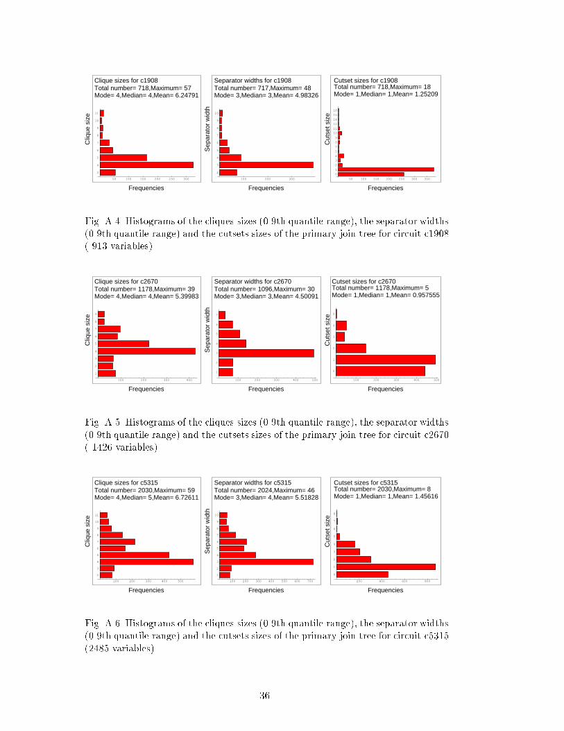
Fig. A.4. Histograms of the cliques sizes (0.9th quantile range), the separator widths(0.9th quantile range) and the cutsets sizes of the primary join tree for circuit c1908( 913 variables).
Frequencies
Cliq
ue s
ize
100 200 300 400
Clique sizes for c2670Total number= 1178,Maximum= 39Mode= 4,Median= 4,Mean= 5.39983
1
2
3
4
5
6
7
8
9
Frequencies
Sep
arat
or w
idth
100 200 300 400 500
Separator widths for c2670Total number= 1096,Maximum= 30Mode= 3,Median= 3,Mean= 4.50091
1
2
3
4
5
6
7
Frequencies
Cut
set s
ize
100 200 300 400 500
Cutset sizes for c2670Total number= 1178,Maximum= 5Mode= 1,Median= 1,Mean= 0.957555
0
1
2
3
4
5
Fig. A.5. Histograms of the cliques sizes (0.9th quantile range), the separator widths(0.9th quantile range) and the cutsets sizes of the primary join tree for circuit c2670( 1426 variables).
Frequencies
Cliq
ue s
ize
100 200 300 400 500
Clique sizes for c5315Total number= 2030,Maximum= 59Mode= 4,Median= 5,Mean= 6.72611
2
3
4
5
6
7
8
9
10
11
Frequencies
Sep
arat
or w
idth
100 200 300 400 500 600 700
Separator widths for c5315Total number= 2024,Maximum= 46Mode= 3,Median= 4,Mean= 5.51828
1
2
3
4
5
6
7
8
9
10
Frequencies
Cut
set s
ize
200 400 600 800
Cutset sizes for c5315Total number= 2030,Maximum= 8Mode= 1,Median= 1,Mean= 1.45616
0
1
2
3
4
5
6
7
8
Fig. A.6. Histograms of the cliques sizes (0.9th quantile range), the separator widths(0.9th quantile range) and the cutsets sizes of the primary join tree for circuit c5315(2485 variables).
36

Frequencies
Cliq
ue s
ize
200 400 600 800
Clique sizes for c6288Total number= 1965,Maximum= 65Mode= 5,Median= 5,Mean= 6.79746
3
4
5
6
7
8
9
10
Frequencies
Sep
arat
or w
idth
200 400 600 800
Separator widths for c6288Total number= 1964,Maximum= 53Mode= 4,Median= 4,Mean= 5.55448
2
3
4
5
6
7
8
9
Frequencies
Cut
set s
ize
200 400 600 800 1000 1200
Cutset sizes for c6288Total number= 1965,Maximum= 8Mode= 1,Median= 1,Mean= 1.06768
0
1
2
3
4
5
6
8
Fig. A.7. Histograms of the cliques sizes (0.9th quantile range), the separator widths(0.9th quantile range) and the cutsets sizes of the primary join tree for circuit c6288(2448 variables).
Table A.1Maximum clique sizes (C) and maximum separator widths (S) for the join treesobtained by tree clustering with various ordering heuristics
Circuit #variables Causal Maximum Minimum Minimum
Ordering Cardinality Width Degree
C S C S C S C S
c17 11 5 3 4 2 4 3 3 2
c432 196 63 62 45 44 51 45 28 23
c499 243 68 66 43 42 33 32 25 18
c880 443 66 64 51 49 66 64 28 21
c1355 587 74 73 47 46 37 36 25 18
c1908 913 139 138 65 63 141 139 57 48
c2670 1426 150 149 82 80 154 152 39 30
c3540 1719 270 269 117 115 294 293 114 89
c5315 2485 172 169 59 46
c6288 2448 277 276 65 53
c7552 3719 58 45
B Ordering Heuristics
As a side e�ect of our experiments we observed a dramatic di�erence be-tween the e�ect of ordering on the resulting primary join tree. In particu-lar the max-cardinality heuristic was shown to be much inferior to the min-degree ordering. Four ordering heuristics were considered: (1) causal ordering,
37

Table A.2Number of added edges (N) and the clustering cpu-seconds (T) for various orderings.
Circuit #var- Causal Maximum Minimum Minimum
iables Ordering Cardinality Width Degree
N T N T N T N T
c17 11 7 0.15 2 0.017 3 0.05 1 0.033
c432 196 7094 154.967 3425 51.916 1895 29.384 869 22.934
c499 243 7348 137.883 3813 65.617 2289 36.633 944 27.483
c880 443 11286 287.067 6788 153.283 9002 257.4 1678 83.634
c1355 587 15241 465.4 9951 302.683 6695 198.433 1272 104.783
c1908 913 60223 4748.73 24445 1147.2 39746 2559.95 4356 418.367
c2670 1426 115519 17457.4 22413 1350.17 60239 5933.17 4381 967.05
c3540 1719 225016 67385.6 64565 5943.72 148251 33038.9 17043 3650.98
c5315 2485 88714 20595.6 11486 5665.68
c6288 2448 291137 1.4805e+05 14311 5415.73
c7552 3719 14968 20301.3
(2) maximum-cardinality, (3) minimum-width, and (4) minimum-degree. Themax-cardinality ordering is computed from �rst to last by picking the �rst nodearbitrarily and then repeatedly selecting the unordered node that is adjacentto the maximum number of already ordered nodes. The min-width ordering iscomputed from last to �rst by repeatedly selecting the node having the leastnumber of neighbors in the graph, removing the node and its incident edgesfrom the graph, and continuing until the graph is empty. The min-degree or-dering is exactly like min-width except that we connect neighbors of selectednodes, and causal ordering is just a topological sort of the DAG.
Tree clustering is implemented using each of the four orderings on each of thebenchmark circuits of table 1. Table A.1 gives the maximum separator widthsand clique sizes for each method on all circuits. We note that among thefour methods, the min-degree ordering has by far the best performance as ityields the smallest cliques sizes and separators. The table shows the maximumseparator widths to be tightly correlated with the maximumclique sizes. As anexample, for circuit c3540, which has 1719 variables, the separator width forthe minimumdegree method is 89. Causal-ordering leads to a separator widththat is 300% greater than the maximumdegree, the maxium-cardinality 130%,and minimum-width 330%. Unlike the three other methods, the minimumdegree leads to separator width that grows only slowly with the size of thecircut. Indeed, the minimum degree was the only method that could scale-up to the largest size circuit. For circuit c6288 (2448 variables) the separator
38

width for minimum-degree is only 53 while with maximum cardinality is 276(520% larger than minimum degree).
Table A.2 gives the number of added edges and the cpu-seconds for clusteringwith each ordering on all circuits. The number of added edges serves as animplementation-independent basis for comparing the e�ciency of the variousclustering methods. The cpu-seconds are tightly correlated with the numberof added edges.
C Structural parameters of secondary trees (Additional data)
Table C.1Structural parameters of primary and secondary trees for c432 (196 variables) ;Max. separator width (Smx), #cliques (N), max clique size (Cmx), max cutset size(CSmx), average separator width (Sav), average clique size (Cav), average cutsetsize (CSav).
Smx N Cmx CSmx Sav Cav CSav
23 157 28 17 6.22436 7.43312 1.92357
20 156 32 21 6.11613 7.33333 1.85897
18 155 33 22 6.02597 7.25161 1.8129
16 151 37 26 5.70667 6.96689 1.6755
11 147 41 30 5.42466 6.72109 1.54422
10 145 43 32 5.34722 6.66207 1.45517
9 144 44 33 5.31469 6.63889 1.41667
8 126 71 35 4.784 6.30159 1.56349
7 117 80 36 4.53448 6.17094 1.62393
6 106 91 37 4.27619 6.08491 1.71698
5 86 111 57 3.87059 6.10465 1.75581
4 65 132 59 3.5 6.46154 1.93846
3 25 172 71 2.66667 10.4 3.64
2 6 191 80 1.4 33.8333 13.5
1 4 193 83 1.0 49.75 20.75
39

Table C.2Structural parameters of primary and secondary trees for c499 (243 variables) ;Max. separator width (Smx), #cliques (N), max clique size (Cmx), max cutset size(CSmx), average separator width (Sav), average clique size (Cav), average cutsetsize (CSav).
Smx N Cmx CSmx Sav Cav CSav
18 196 25 8 4.86667 6.08163 1.45918
17 192 29 8 4.59162 5.83333 1.47917
12 189 49 11 4.39362 5.65608 1.4127
8 179 59 18 3.96629 5.30168 1.45251
6 171 67 18 3.77647 5.17544 1.52047
5 155 83 28 3.54545 5.09032 1.38065
4 105 139 56 2.84615 5.13333 1.52381
3 81 163 74 2.5 5.46914 1.90123
2 41 203 78 2.0 7.87805 2.87805
40
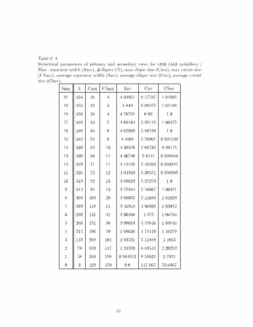
Table C.3Structural parameters of primary and secondary trees for c880 (443 variables) ;Max. separator width (Smx), #cliques (N), max clique size (Cmx), max cutset size(CSmx), average separator width (Sav), average clique size (Cav), average cutsetsize (CSav).
Smx N Cmx CSmx Sav Cav CSav
21 354 28 4 4.94051 6.17797 1.01695
19 352 32 4 4.849 6.09375 1.01136
18 350 34 4 4.76791 6.02 1.0
17 348 43 5 4.69164 5.95115 1.00575
16 346 45 6 4.62029 5.88728 1.0
15 342 58 9 4.4868 5.76901 0.991228
14 339 62 10 4.39349 5.68732 0.99115
13 336 66 11 4.30746 5.6131 0.994048
12 329 71 11 4.12195 5.45593 0.993921
11 326 75 12 4.04923 5.39571 0.993865
10 319 82 13 3.89623 5.27273 1.0
9 312 88 13 3.75884 5.16667 1.00321
8 308 103 20 3.69055 5.11688 1.01623
7 293 118 24 3.46918 4.96928 1.03072
6 280 131 31 3.30466 4.875 1.06786
5 260 151 36 3.09653 4.78846 1.08846
4 215 196 59 2.69626 4.74419 1.16279
3 143 268 104 2.03521 5.11888 1.4965
2 79 349 147 1.24359 6.83544 2.20253
1 58 380 158 0.964912 8.58621 2.7931
0 3 429 159 0.0 147.667 53.6667
41

Table C.4Structural parameters of primary and secondary trees for c1355 (587 variables) ;Max. separator width (Smx), #cliques (N), max clique size (Cmx), max cutset size(CSmx), average separator width (Sav), average clique size (Cav), average cutsetsize (CSav).
Smx N Cmx CSmx Sav Cav CSav
18 436 25 11 3.8 5.13761 1.18349
17 432 29 11 3.66821 5.01852 1.18981
12 429 49 11 3.57477 4.93473 1.14452
8 419 59 18 3.37321 4.76611 1.15513
6 411 67 18 3.28293 4.70316 1.17762
5 395 83 28 3.17259 4.65063 1.10886
4 345 139 44 2.90698 4.6 1.14783
3 241 163 44 2.43333 4.85892 1.64315
2 105 419 203 1.69231 7.26667 2.92381
1 33 555 235 1.0 18.7576 7.12121
42

Table C.5Structural parameters of primary and secondary trees for c1908 (913 variables) ;Max. separator width (Smx), #cliques (N), max clique size (Cmx), max cutset size(CSmx), average separator width (Sav), average clique size (Cav), average cutsetsize (CSav).
Smx N Cmx CSmx Sav Cav CSav
48 718 57 18 4.98326 6.24791 1.25209
42 717 65 18 4.92318 6.18968 1.2371
40 716 68 18 4.87133 6.13966 1.22765
38 715 69 18 4.82213 6.09231 1.21958
35 712 74 18 4.68214 5.95787 1.18399
33 711 76 19 4.63944 5.91702 1.16596
31 710 77 20 4.59944 5.87887 1.1493
29 708 82 20 4.52475 5.80791 1.13418
25 707 83 20 4.49008 5.77511 1.12447
24 706 84 20 4.46099 5.74788 1.12323
23 704 88 22 4.40541 5.69602 1.11222
22 703 90 22 4.37892 5.67141 1.10953
19 701 92 22 4.32857 5.62482 1.10271
18 700 94 22 4.30758 5.60571 1.09857
16 696 100 24 4.22878 5.53448 1.08333
15 692 104 25 4.16064 5.47399 1.05925
14 678 118 39 3.93648 5.27729 0.914454
13 666 130 46 3.75489 5.12012 0.795796
12 660 138 46 3.67071 5.04848 0.777273
11 656 143 48 3.61985 5.0061 0.778963
10 654 145 50 3.59724 4.98777 0.776758
9 642 158 52 3.47738 4.89408 0.758567
8 635 166 54 3.4164 4.84882 0.76378
7 627 174 54 3.35783 4.80861 0.767145
6 618 185 55 3.3047 4.7767 0.775081
5 587 217 60 3.16212 4.7121 0.749574
4 548 258 62 3.03108 4.69161 0.775547
3 460 350 76 2.84532 4.82391 0.897826
2 72 788 296 2.0 14.6528 4.95833
43
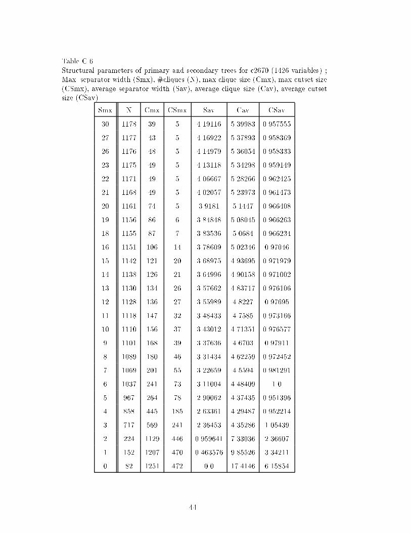
Table C.6Structural parameters of primary and secondary trees for c2670 (1426 variables) ;Max. separator width (Smx), #cliques (N), max clique size (Cmx), max cutset size(CSmx), average separator width (Sav), average clique size (Cav), average cutsetsize (CSav).
Smx N Cmx CSmx Sav Cav CSav
30 1178 39 5 4.19116 5.39983 0.957555
27 1177 43 5 4.16922 5.37893 0.958369
26 1176 48 5 4.14979 5.36054 0.958333
23 1175 49 5 4.13118 5.34298 0.959149
22 1171 49 5 4.06667 5.28266 0.962425
21 1168 49 5 4.02057 5.23973 0.961473
20 1161 74 5 3.9181 5.1447 0.966408
19 1156 86 6 3.84848 5.08045 0.966263
18 1155 87 7 3.83536 5.0684 0.966234
16 1151 106 14 3.78609 5.02346 0.97046
15 1142 121 20 3.68975 4.93695 0.971979
14 1138 126 21 3.64996 4.90158 0.971002
13 1130 134 26 3.57662 4.83717 0.976106
12 1128 136 27 3.55989 4.8227 0.97695
11 1118 147 32 3.48433 4.7585 0.973166
10 1110 156 37 3.43012 4.71351 0.976577
9 1101 168 39 3.37636 4.6703 0.97911
8 1089 180 46 3.31434 4.62259 0.972452
7 1069 201 55 3.22659 4.5594 0.981291
6 1037 241 73 3.11004 4.48409 1.0
5 967 264 78 2.90062 4.37435 0.951396
4 858 445 185 2.63361 4.29487 0.952214
3 717 569 241 2.36453 4.35286 1.05439
2 224 1129 446 0.959641 7.33036 2.36607
1 152 1207 470 0.463576 9.85526 3.34211
0 82 1251 472 0.0 17.4146 6.15854
44
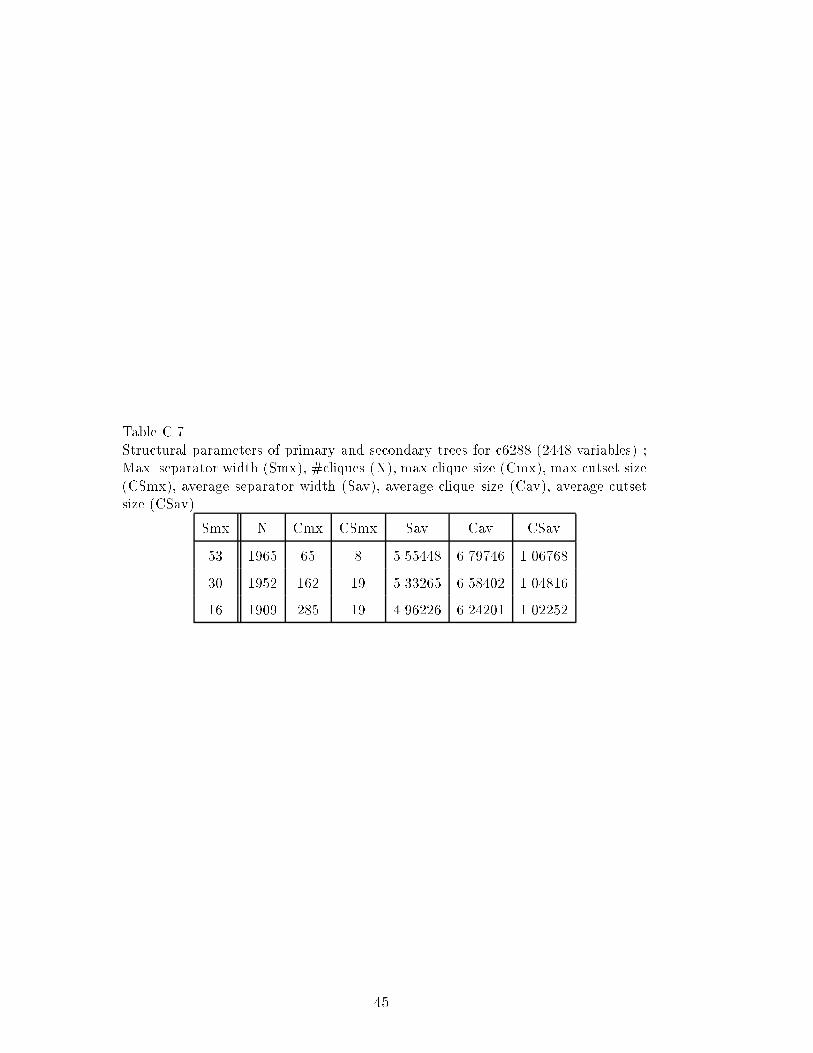
Table C.7Structural parameters of primary and secondary trees for c6288 (2448 variables) ;Max. separator width (Smx), #cliques (N), max clique size (Cmx), max cutset size(CSmx), average separator width (Sav), average clique size (Cav), average cutsetsize (CSav).
Smx N Cmx CSmx Sav Cav CSav
53 1965 65 8 5.55448 6.79746 1.06768
30 1952 162 19 5.33265 6.58402 1.04816
16 1909 285 19 4.96226 6.24201 1.02252
45


![Optimization of Electrical Discharge Machining Process ... · ptimization of Electrical Discharge Machining Process arameters Using Flushing and Drilled Tool Rahul Gupta 1, ... (EDM)[1]](https://img.dokumen.tips/doc/110x75/5e9599204c173d796756a013/optimization-of-electrical-discharge-machining-process-ptimization-of-electrical.jpg)