Embed Size (px)
Citation preview
1
C H A P T E R 1
Systems of LinearEquations and Matrices
CHAPTER CONTENTS 1.1 Introduction to Systems of Linear Equations 2
1.2 Gaussian Elimination 11
1.3 Matrices and Matrix Operations 25
1.4 Inverses; Algebraic Properties of Matrices 39
1.5 Elementary Matrices and a Method for Finding A−1 52
1.6 More on Linear Systems and Invertible Matrices 61
1.7 Diagonal,Triangular, and Symmetric Matrices 67
1.8 MatrixTransformations 75
1.9 Applications of Linear Systems 84
• Network Analysis (Traffic Flow) 84
• Electrical Circuits 86
• Balancing Chemical Equations 88
• Polynomial Interpolation 91
1.10 Leontief Input-Output Models 96
INTRODUCTION Information in science, business, and mathematics is often organized into rows andcolumns to form rectangular arrays called “matrices” (plural of “matrix”). Matricesoften appear as tables of numerical data that arise from physical observations, but theyoccur in various mathematical contexts as well. For example, we will see in this chapterthat all of the information required to solve a system of equations such as
5x + y = 3
2x − y = 4
is embodied in the matrix [5
2
1
−1
3
4
]and that the solution of the system can be obtained by performing appropriateoperations on this matrix. This is particularly important in developing computerprograms for solving systems of equations because computers are well suited formanipulating arrays of numerical information. However, matrices are not simply anotational tool for solving systems of equations; they can be viewed as mathematicalobjects in their own right, and there is a rich and important theory associated withthem that has a multitude of practical applications. It is the study of matrices andrelated topics that forms the mathematical field that we call “linear algebra.” In thischapter we will begin our study of matrices.
2 Chapter 1 Systems of Linear Equations and Matrices
1.1 Introduction to Systems of Linear EquationsSystems of linear equations and their solutions constitute one of the major topics that wewill study in this course. In this first section we will introduce some basic terminology anddiscuss a method for solving such systems.
Linear Equations Recall that in two dimensions a line in a rectangular xy-coordinate system can be repre-sented by an equation of the form
ax + by = c (a, b not both 0)
and in three dimensions a plane in a rectangular xyz-coordinate system can be repre-sented by an equation of the form
ax + by + cz = d (a, b, c not all 0)
These are examples of “linear equations,” the first being a linear equation in the variablesx and y and the second a linear equation in the variables x, y, and z. More generally, wedefine a linear equation in the n variables x1, x2, . . . , xn to be one that can be expressedin the form
a1x1 + a2x2 + · · · + anxn = b (1)
where a1, a2, . . . , an and b are constants, and the a’s are not all zero. In the special caseswhere n = 2 or n = 3, we will often use variables without subscripts and write linearequations as
a1x + a2y = b (a1, a2 not both 0) (2)
a1x + a2y + a3z = b (a1, a2, a3 not all 0) (3)
In the special case where b = 0, Equation (1) has the form
a1x1 + a2x2 + · · · + anxn = 0 (4)
which is called a homogeneous linear equation in the variables x1, x2, . . . , xn.
EXAMPLE 1 Linear Equations
Observe that a linear equation does not involve any products or roots of variables. Allvariables occur only to the first power and do not appear, for example, as arguments oftrigonometric, logarithmic, or exponential functions. The following are linear equations:
x + 3y = 7 x1 − 2x2 − 3x3 + x4 = 012 x − y + 3z = −1 x1 + x2 + · · · + xn = 1
The following are not linear equations:
x + 3y2 = 4 3x + 2y − xy = 5
sin x + y = 0√
x1 + 2x2 + x3 = 1
A finite set of linear equations is called a system of linear equations or, more briefly,a linear system. The variables are called unknowns. For example, system (5) that followshas unknowns x and y, and system (6) has unknowns x1, x2, and x3.
5x + y = 3 4x1 − x2 + 3x3 = −12x − y = 4 3x1 + x2 + 9x3 = −4
(5–6)
1.1 Introduction to Systems of Linear Equations 3
A general linear system of m equations in the n unknowns x1, x2, . . . , xn can be writtenThe double subscripting onthe coefficients aij of the un-knowns gives their locationin the system—the first sub-script indicates the equationin which the coefficient occurs,and the second indicates whichunknown it multiplies. Thus,a12 is in the first equation andmultiplies x2.
asa11x1 + a12x2 + · · · + a1nxn = b1
a21x1 + a22x2 + · · · + a2nxn = b2...
......
...am1x1 + am2x2 + · · · + amnxn = bm
(7)
A solution of a linear system in n unknowns x1, x2, . . . , xn is a sequence of n numberss1, s2, . . . , sn for which the substitution
x1 = s1, x2 = s2, . . . , xn = sn
makes each equation a true statement. For example, the system in (5) has the solution
x = 1, y = −2
and the system in (6) has the solution
x1 = 1, x2 = 2, x3 = −1
These solutions can be written more succinctly as
(1,−2) and (1, 2,−1)
in which the names of the variables are omitted. This notation allows us to interpretthese solutions geometrically as points in two-dimensional and three-dimensional space.More generally, a solution
x1 = s1, x2 = s2, . . . , xn = sn
of a linear system in n unknowns can be written as
(s1, s2, . . . , sn)
which is called an ordered n-tuple. With this notation it is understood that all variablesappear in the same order in each equation. If n = 2, then the n-tuple is called an orderedpair, and if n = 3, then it is called an ordered triple.
Linear Systems inTwo andThree Unknowns
Linear systems in two unknowns arise in connection with intersections of lines. Forexample, consider the linear system
a1x + b1y = c1
a2x + b2y = c2
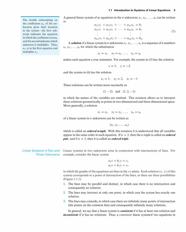
in which the graphs of the equations are lines in the xy-plane. Each solution (x, y) of thissystem corresponds to a point of intersection of the lines, so there are three possibilities(Figure 1.1.1):
1. The lines may be parallel and distinct, in which case there is no intersection andconsequently no solution.
2. The lines may intersect at only one point, in which case the system has exactly onesolution.
3. The lines may coincide, in which case there are infinitely many points of intersection(the points on the common line) and consequently infinitely many solutions.
In general, we say that a linear system is consistent if it has at least one solution andinconsistent if it has no solutions. Thus, a consistent linear systemof two equations in
4 Chapter 1 Systems of Linear Equations and Matrices
Figure 1.1.1
x
y
No solution
x
y
One solution
x
y
Infinitely many
solutions
(coincident lines)
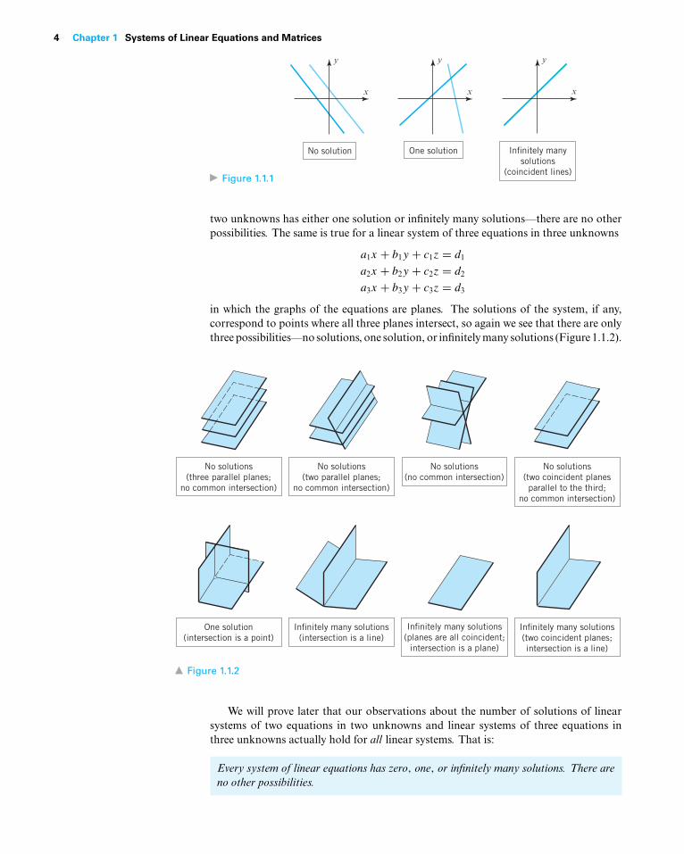
two unknowns has either one solution or infinitely many solutions—there are no otherpossibilities. The same is true for a linear system of three equations in three unknowns
a1x + b1y + c1z = d1
a2x + b2y + c2z = d2
a3x + b3y + c3z = d3
in which the graphs of the equations are planes. The solutions of the system, if any,correspond to points where all three planes intersect, so again we see that there are onlythree possibilities—no solutions, one solution, or infinitely many solutions (Figure 1.1.2).
No solutions
(three parallel planes;
no common intersection)
No solutions
(two parallel planes;
no common intersection)
No solutions
(no common intersection)
Infinitely many solutions
(planes are all coincident;
intersection is a plane)
Infinitely many solutions
(intersection is a line)
One solution
(intersection is a point)
No solutions
(two coincident planes
parallel to the third;
no common intersection)
Infinitely many solutions
(two coincident planes;
intersection is a line)
Figure 1.1.2
We will prove later that our observations about the number of solutions of linearsystems of two equations in two unknowns and linear systems of three equations inthree unknowns actually hold for all linear systems. That is:
Every system of linear equations has zero, one, or infinitely many solutions. There areno other possibilities.
1.1 Introduction to Systems of Linear Equations 5
EXAMPLE 2 A Linear System with One Solution
Solve the linear systemx − y = 1
2x + y = 6
Solution We can eliminate x from the second equation by adding −2 times the firstequation to the second. This yields the simplified system
x − y = 1
3y = 4
From the second equation we obtain y = 43 , and on substituting this value in the first
equation we obtain x = 1 + y = 73 . Thus, the system has the unique solution
x = 73 , y = 4
3
Geometrically, this means that the lines represented by the equations in the systemintersect at the single point
(73 , 4
3
). We leave it for you to check this by graphing the
lines.
EXAMPLE 3 A Linear System with No Solutions
Solve the linear systemx + y = 4
3x + 3y = 6
Solution We can eliminate x from the second equation by adding −3 times the firstequation to the second equation. This yields the simplified system
x + y = 4
0 = −6
The second equation is contradictory, so the given system has no solution. Geometrically,this means that the lines corresponding to the equations in the original system are paralleland distinct. We leave it for you to check this by graphing the lines or by showing thatthey have the same slope but different y-intercepts.
EXAMPLE 4 A Linear System with Infinitely Many Solutions
Solve the linear system4x − 2y = 1
16x − 8y = 4
Solution We can eliminate x from the second equation by adding −4 times the firstequation to the second. This yields the simplified system
4x − 2y = 1
0 = 0
The second equation does not impose any restrictions on x and y and hence can beomitted. Thus, the solutions of the system are those values of x and y that satisfy thesingle equation
4x − 2y = 1 (8)
Geometrically, this means the lines corresponding to the two equations in the originalsystem coincide. One way to describe the solution set is to solve this equation for x interms of y to obtain x = 1
4 + 12 y and then assign an arbitrary value t (called a parameter)
6 Chapter 1 Systems of Linear Equations and Matrices
to y. This allows us to express the solution by the pair of equations (called parametricequations)
x = 14 + 1
2 t, y = t
We can obtain specific numerical solutions from these equations by substituting numer-
In Example 4 we could havealso obtained parametricequations for the solutionsby solving (8) for y in termsof x and letting x = t bethe parameter. The resultingparametric equations wouldlook different but woulddefine the same solution set.
ical values for the parameter t . For example, t = 0 yields the solution(
14 , 0
), t = 1
yields the solution(
34 , 1
), and t = −1 yields the solution
(− 14 ,−1
). You can confirm
that these are solutions by substituting their coordinates into the given equations.
EXAMPLE 5 A Linear System with Infinitely Many Solutions
Solve the linear systemx − y + 2z = 5
2x − 2y + 4z = 10
3x − 3y + 6z = 15
Solution This system can be solved by inspection, since the second and third equationsare multiples of the first. Geometrically, this means that the three planes coincide andthat those values of x, y, and z that satisfy the equation
x − y + 2z = 5 (9)
automatically satisfy all three equations. Thus, it suffices to find the solutions of (9).We can do this by first solving this equation for x in terms of y and z, then assigningarbitrary values r and s (parameters) to these two variables, and then expressing thesolution by the three parametric equations
x = 5 + r − 2s, y = r, z = s
Specific solutions can be obtained by choosing numerical values for the parameters r
and s. For example, taking r = 1 and s = 0 yields the solution (6, 1, 0).
Augmented Matrices andElementary Row Operations
As the number of equations and unknowns in a linear system increases, so does thecomplexity of the algebra involved in finding solutions. The required computations canbe made more manageable by simplifying notation and standardizing procedures. Forexample, by mentally keeping track of the location of the +’s, the x’s, and the =’s in thelinear system
a11x1 + a12x2 + · · ·+ a1nxn = b1
a21x1 + a22x2 + · · ·+ a2nxn = b2...
......
...am1x1 + am2x2 + · · ·+ amnxn = bm
we can abbreviate the system by writing only the rectangular array of numbers⎡⎢⎢⎢⎣
a11 a12 · · · a1n b1
a21 a22 · · · a2n b2...
......
...am1 am2 · · · amn bm
⎤⎥⎥⎥⎦
This is called the augmented matrix for the system. For example, the augmented matrix
As noted in the introductionto this chapter, the term “ma-trix” is used in mathematics todenote a rectangular array ofnumbers. In a later sectionwe will study matrices in de-tail, but for now we will onlybe concerned with augmentedmatrices for linear systems.
for the system of equations
x1 + x2 + 2x3 = 9
2x1 + 4x2 − 3x3 = 1
3x1 + 6x2 − 5x3 = 0
is
⎡⎢⎣1 1 2 9
2 4 −3 1
3 6 −5 0
⎤⎥⎦
1.1 Introduction to Systems of Linear Equations 7
The basic method for solving a linear system is to perform algebraic operations onthe system that do not alter the solution set and that produce a succession of increasinglysimpler systems, until a point is reached where it can be ascertained whether the systemis consistent, and if so, what its solutions are. Typically, the algebraic operations are:
1. Multiply an equation through by a nonzero constant.
2. Interchange two equations.
3. Add a constant times one equation to another.
Since the rows (horizontal lines) of an augmented matrix correspond to the equations inthe associated system, these three operations correspond to the following operations onthe rows of the augmented matrix:
1. Multiply a row through by a nonzero constant.
2. Interchange two rows.
3. Add a constant times one row to another.
These are called elementary row operations on a matrix.In the following example we will illustrate how to use elementary row operations and
an augmented matrix to solve a linear system in three unknowns. Since a systematicprocedure for solving linear systems will be developed in the next section, do not worryabout how the steps in the example were chosen. Your objective here should be simplyto understand the computations.
EXAMPLE 6 Using Elementary Row Operations
In the left column we solve a system of linear equations by operating on the equations inthe system, and in the right column we solve the same system by operating on the rowsof the augmented matrix.
x + y + 2z = 9
2x + 4y − 3z = 1
3x + 6y − 5z = 0
⎡⎢⎣1 1 2 9
2 4 −3 1
3 6 −5 0
⎤⎥⎦
Add −2 times the first equation to the secondto obtain
x + y + 2z = 9
2y − 7z = −17
3x + 6y − 5z = 0
Add −2 times the first row to the second toobtain ⎡
⎢⎣1 1 2 9
0 2 −7 −17
3 6 −5 0
⎤⎥⎦
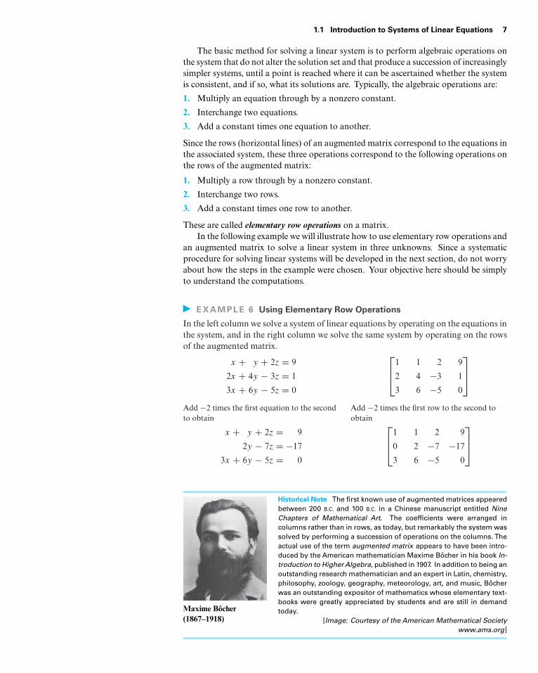
Maxime Bôcher(1867–1918)
Historical Note The first known use of augmented matrices appearedbetween 200 B.C. and 100 B.C. in a Chinese manuscript entitled NineChapters of Mathematical Art. The coefficients were arranged incolumns rather than in rows, as today, but remarkably the system wassolved by performing a succession of operations on the columns. Theactual use of the term augmented matrix appears to have been intro-duced by the American mathematician Maxime Bôcher in his book In-troduction to HigherAlgebra, published in 1907. In addition to being anoutstanding research mathematician and an expert in Latin, chemistry,philosophy, zoology, geography, meteorology, art, and music, Bôcherwas an outstanding expositor of mathematics whose elementary text-books were greatly appreciated by students and are still in demandtoday.
[Image: Courtesy of the American Mathematical Societywww.ams.org]
8 Chapter 1 Systems of Linear Equations and Matrices
Add −3 times the first equation to the third toobtain
x + y + 2z = 9
2y − 7z = −17
3y − 11z = −27
Add−3 times the first row to the third to obtain
⎡⎢⎣1 1 2 9
0 2 −7 −17
0 3 −11 −27
⎤⎥⎦
Multiply the second equation by 12 to obtain
x + y + 2z = 9
y − 72z = − 17
2
3y − 11z = −27
Multiply the second row by 12 to obtain⎡
⎢⎣1 1 2 9
0 1 − 72 − 17
2
0 3 −11 −27
⎤⎥⎦
Add −3 times the second equation to the thirdto obtain
x + y + 2z = 9
y − 72z = − 17
2
− 12z = − 3
2
Add −3 times the second row to the third toobtain ⎡
⎢⎢⎣1 1 2 9
0 1 − 72 − 17
2
0 0 − 12 − 3
2
⎤⎥⎥⎦
Multiply the third equation by −2 to obtain
x + y + 2z = 9
y − 72z = − 17
2
z = 3
Multiply the third row by −2 to obtain⎡⎢⎣1 1 2 9
0 1 − 72 − 17
2
0 0 1 3
⎤⎥⎦
Add −1 times the second equation to the firstto obtain
x + 112 z = 35
2
y − 72z = − 17
2
z = 3
Add −1 times the second row to the first toobtain ⎡
⎢⎢⎣1 0 11
2352
0 1 − 72 − 17
2
0 0 1 3
⎤⎥⎥⎦
Add −112 times the third equation to the first
and 72 times the third equation to the second to
obtainx = 1
y = 2
z = 3
Add − 112 times the third row to the first and 7
2
times the third row to the second to obtain⎡⎢⎣1 0 0 1
0 1 0 2
0 0 1 3
⎤⎥⎦
The solution x = 1, y = 2, z = 3 is now evident.
The solution in this examplecan also be expressed as the or-dered triple (1, 2, 3) with theunderstanding that the num-bers in the triple are in thesame order as the variables inthe system, namely, x, y, z.
Exercise Set 1.11. In each part, determine whether the equation is linear in x1,
x2, and x3.
(a) x1 + 5x2 − √2 x3 = 1 (b) x1 + 3x2 + x1x3 = 2
(c) x1 = −7x2 + 3x3 (d) x−21 + x2 + 8x3 = 5
(e) x3/51 − 2x2 + x3 = 4 (f ) πx1 −
√2 x2 = 71/3
2. In each part, determine whether the equation is linear in x
and y.
(a) 21/3x +√3y = 1 (b) 2x1/3 + 3
√y = 1
(c) cos(
π
7
)x − 4y = log 3 (d) π
7 cos x − 4y = 0
(e) xy = 1 (f ) y + 7 = x
1.1 Introduction to Systems of Linear Equations 9
3. Using the notation of Formula (7), write down a general linearsystem of
(a) two equations in two unknowns.
(b) three equations in three unknowns.
(c) two equations in four unknowns.
4. Write down the augmented matrix for each of the linear sys-tems in Exercise 3.
In each part of Exercises 5–6, find a linear system in the un-knowns x1, x2, x3, . . . , that corresponds to the given augmentedmatrix.
5. (a)
⎡⎢⎣2 0 0
3 −4 0
0 1 1
⎤⎥⎦ (b)
⎡⎢⎣3 0 −2 5
7 1 4 −3
0 −2 1 7
⎤⎥⎦
6. (a)
[0 3 −1 −1 −1
5 2 0 −3 −6
]
(b)
⎡⎢⎢⎢⎣
3 0 1 −4 3
−4 0 4 1 −3
−1 3 0 −2 −9
0 0 0 −1 −2
⎤⎥⎥⎥⎦
In each part of Exercises 7–8, find the augmented matrix forthe linear system.
7. (a) −2x1 = 63x1 = 89x1 = −3
(b) 6x1 − x2 + 3x3 = 45x2 − x3 = 1
(c) 2x2 − 3x4 + x5 = 0−3x1 − x2 + x3 = −1
6x1 + 2x2 − x3 + 2x4 − 3x5 = 6
8. (a) 3x1 − 2x2 = −14x1 + 5x2 = 37x1 + 3x2 = 2
(b) 2x1 + 2x3 = 13x1 − x2 + 4x3 = 76x1 + x2 − x3 = 0
(c) x1 = 1x2 = 2
x3 = 3
9. In each part, determine whether the given 3-tuple is a solutionof the linear system
2x1 − 4x2 − x3 = 1x1 − 3x2 + x3 = 1
3x1 − 5x2 − 3x3 = 1
(a) (3, 1, 1) (b) (3,−1, 1) (c) (13, 5, 2)
(d)(
132 , 5
2 , 2)
(e) (17, 7, 5)
10. In each part, determine whether the given 3-tuple is a solutionof the linear system
x + 2y − 2z = 33x − y + z = 1−x + 5y − 5z = 5
(a)(
57 ,
87 , 1
)(b)
(57 ,
87 , 0
)(c) (5, 8, 1)
(d)(
57 ,
107 , 2
7
)(e)
(57 ,
227 , 2
)11. In each part, solve the linear system, if possible, and use the
result to determine whether the lines represented by the equa-tions in the system have zero, one, or infinitely many points ofintersection. If there is a single point of intersection, give itscoordinates, and if there are infinitely many, find parametricequations for them.
(a) 3x − 2y = 46x − 4y = 9
(b) 2x − 4y = 14x − 8y = 2
(c) x − 2y = 0x − 4y = 8
12. Under what conditions on a and b will the following linearsystem have no solutions, one solution, infinitely many solu-tions?
2x − 3y = a
4x − 6y = b
In each part of Exercises 13–14, use parametric equations todescribe the solution set of the linear equation.
13. (a) 7x − 5y = 3
(b) 3x1 − 5x2 + 4x3 = 7
(c) −8x1 + 2x2 − 5x3 + 6x4 = 1
(d) 3v − 8w + 2x − y + 4z = 0
14. (a) x + 10y = 2
(b) x1 + 3x2 − 12x3 = 3
(c) 4x1 + 2x2 + 3x3 + x4 = 20
(d) v + w + x − 5y + 7z = 0
In Exercises 15–16, each linear system has infinitely many so-lutions. Use parametric equations to describe its solution set.
15. (a) 2x − 3y = 16x − 9y = 3
(b) x1 + 3x2 − x3 = −43x1 + 9x2 − 3x3 = −12−x1 − 3x2 + x3 = 4
16. (a) 6x1 + 2x2 = −83x1 + x2 = −4
(b) 2x − y + 2z = −46x − 3y + 6z = −12
−4x + 2y − 4z = 8
In Exercises 17–18, find a single elementary row operation thatwill create a 1 in the upper left corner of the given augmented ma-trix and will not create any fractions in its first row.
17. (a)
⎡⎣−3 −1 2 4
2 −3 3 20 2 −3 1
⎤⎦ (b)
⎡⎣0 −1 −5 0
2 −9 3 21 4 −3 3
⎤⎦
18. (a)
⎡⎣ 2 4 −6 8
7 1 4 3−5 4 2 7
⎤⎦ (b)
⎡⎣ 7 −4 −2 2
3 −1 8 1−6 3 −1 4
⎤⎦
10 Chapter 1 Systems of Linear Equations and Matrices
In Exercises 19–20, find all values of k for which the givenaugmented matrix corresponds to a consistent linear system.
19. (a)
[1 k −44 8 2
](b)
[1 k −14 8 −4
]
20. (a)
[3 −4 k
−6 8 5
](b)
[k 1 −24 −1 2
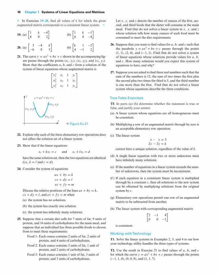
]21. The curve y = ax2 + bx + c shown in the accompanying fig-
ure passes through the points (x1, y1), (x2, y2), and (x3, y3).Show that the coefficients a, b, and c form a solution of thesystem of linear equations whose augmented matrix is⎡
⎢⎣x2
1 x1 1 y1
x22 x2 1 y2
x23 x3 1 y3
⎤⎥⎦
y
x
y = ax2 + bx + c
(x1, y1)
(x3, y3)
(x2, y2)
Figure Ex-21
22. Explain why each of the three elementary row operations doesnot affect the solution set of a linear system.
23. Show that if the linear equations
x1 + kx2 = c and x1 + lx2 = d
have the same solution set, then the two equations are identical(i.e., k = l and c = d).
24. Consider the system of equations
ax + by = k
cx + dy = l
ex + fy = m
Discuss the relative positions of the lines ax + by = k,cx + dy = l, and ex + fy = m when
(a) the system has no solutions.
(b) the system has exactly one solution.
(c) the system has infinitely many solutions.
25. Suppose that a certain diet calls for 7 units of fat, 9 units ofprotein, and 16 units of carbohydrates for the main meal, andsuppose that an individual has three possible foods to choosefrom to meet these requirements:
Food 1: Each ounce contains 2 units of fat, 2 units ofprotein, and 4 units of carbohydrates.
Food 2: Each ounce contains 3 units of fat, 1 unit ofprotein, and 2 units of carbohydrates.
Food 3: Each ounce contains 1 unit of fat, 3 units ofprotein, and 5 units of carbohydrates.
Let x, y, and z denote the number of ounces of the first, sec-ond, and third foods that the dieter will consume at the mainmeal. Find (but do not solve) a linear system in x, y, and z
whose solution tells how many ounces of each food must beconsumed to meet the diet requirements.
26. Suppose that you want to find values for a, b, and c such thatthe parabola y = ax2 + bx + c passes through the points(1, 1), (2, 4), and (−1, 1). Find (but do not solve) a systemof linear equations whose solutions provide values for a, b,
and c. How many solutions would you expect this system ofequations to have, and why?
27. Suppose you are asked to find three real numbers such that thesum of the numbers is 12, the sum of two times the first plusthe second plus two times the third is 5, and the third numberis one more than the first. Find (but do not solve) a linearsystem whose equations describe the three conditions.
True-False Exercises
TF. In parts (a)–(h) determine whether the statement is true orfalse, and justify your answer.
(a) A linear system whose equations are all homogeneous mustbe consistent.
(b) Multiplying a row of an augmented matrix through by zero isan acceptable elementary row operation.
(c) The linear systemx − y = 3
2x − 2y = k
cannot have a unique solution, regardless of the value of k.
(d) A single linear equation with two or more unknowns musthave infinitely many solutions.
(e) If the number of equations in a linear system exceeds the num-ber of unknowns, then the system must be inconsistent.
(f ) If each equation in a consistent linear system is multipliedthrough by a constant c, then all solutions to the new systemcan be obtained by multiplying solutions from the originalsystem by c.
(g) Elementary row operations permit one row of an augmentedmatrix to be subtracted from another.
(h) The linear system with corresponding augmented matrix[2 −1 40 0 −1
]is consistent.
Working withTechnology
T1. Solve the linear systems in Examples 2, 3, and 4 to see howyour technology utility handles the three types of systems.
T2. Use the result in Exercise 21 to find values of a, b, and c
for which the curve y = ax2 + bx + c passes through the points(−1, 1, 4), (0, 0, 8), and (1, 1, 7).
1.2 Gaussian Elimination 11
1.2 Gaussian EliminationIn this section we will develop a systematic procedure for solving systems of linearequations. The procedure is based on the idea of performing certain operations on the rowsof the augmented matrix that simplify it to a form from which the solution of the systemcan be ascertained by inspection.
Considerations in SolvingLinear Systems
When considering methods for solving systems of linear equations, it is important todistinguish between large systems that must be solved by computer and small systemsthat can be solved by hand. For example, there are many applications that lead tolinear systems in thousands or even millions of unknowns. Large systems require specialtechniques to deal with issues of memory size, roundoff errors, solution time, and soforth. Such techniques are studied in the field of numerical analysis and will only betouched on in this text. However, almost all of the methods that are used for largesystems are based on the ideas that we will develop in this section.
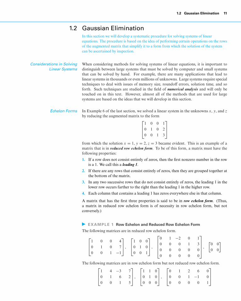
Echelon Forms In Example 6 of the last section, we solved a linear system in the unknowns x, y, and z
by reducing the augmented matrix to the form⎡⎢⎣1 0 0 1
0 1 0 2
0 0 1 3
⎤⎥⎦
from which the solution x = 1, y = 2, z = 3 became evident. This is an example of amatrix that is in reduced row echelon form. To be of this form, a matrix must have thefollowing properties:
1. If a row does not consist entirely of zeros, then the first nonzero number in the rowis a 1. We call this a leading 1.
2. If there are any rows that consist entirely of zeros, then they are grouped together atthe bottom of the matrix.
3. In any two successive rows that do not consist entirely of zeros, the leading 1 in thelower row occurs farther to the right than the leading 1 in the higher row.
4. Each column that contains a leading 1 has zeros everywhere else in that column.
A matrix that has the first three properties is said to be in row echelon form. (Thus,a matrix in reduced row echelon form is of necessity in row echelon form, but notconversely.)
EXAMPLE 1 Row Echelon and Reduced Row Echelon Form
The following matrices are in reduced row echelon form.⎡⎢⎣1 0 0 4
0 1 0 7
0 0 1 −1
⎤⎥⎦ ,
⎡⎢⎣1 0 0
0 1 0
0 0 1
⎤⎥⎦ ,
⎡⎢⎢⎢⎣
0 1 −2 0 1
0 0 0 1 3
0 0 0 0 0
0 0 0 0 0
⎤⎥⎥⎥⎦ ,
[0 0
0 0
]
The following matrices are in row echelon form but not reduced row echelon form.⎡⎢⎣1 4 −3 7
0 1 6 2
0 0 1 5
⎤⎥⎦ ,
⎡⎢⎣1 1 0
0 1 0
0 0 0
⎤⎥⎦ ,
⎡⎢⎣0 1 2 6 0
0 0 1 −1 0
0 0 0 0 1
⎤⎥⎦
12 Chapter 1 Systems of Linear Equations and Matrices
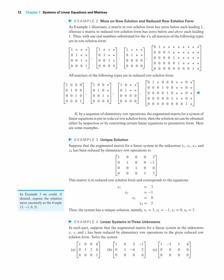
EXAMPLE 2 More on Row Echelon and Reduced Row Echelon Form
As Example 1 illustrates, a matrix in row echelon form has zeros below each leading 1,whereas a matrix in reduced row echelon form has zeros below and above each leading1. Thus, with any real numbers substituted for the ∗’s, all matrices of the following typesare in row echelon form:⎡⎢⎢⎢⎣
1 ∗ ∗ ∗0 1 ∗ ∗0 0 1 ∗0 0 0 1
⎤⎥⎥⎥⎦ ,
⎡⎢⎢⎢⎣
1 ∗ ∗ ∗0 1 ∗ ∗0 0 1 ∗0 0 0 0
⎤⎥⎥⎥⎦ ,
⎡⎢⎢⎢⎣
1 ∗ ∗ ∗0 1 ∗ ∗0 0 0 0
0 0 0 0
⎤⎥⎥⎥⎦ ,
⎡⎢⎢⎢⎢⎢⎣
0 1 ∗ ∗ ∗ ∗ ∗ ∗ ∗ ∗0 0 0 1 ∗ ∗ ∗ ∗ ∗ ∗0 0 0 0 1 ∗ ∗ ∗ ∗ ∗0 0 0 0 0 1 ∗ ∗ ∗ ∗0 0 0 0 0 0 0 0 1 ∗
⎤⎥⎥⎥⎥⎥⎦
All matrices of the following types are in reduced row echelon form:
⎡⎢⎢⎢⎣
1 0 0 0
0 1 0 0
0 0 1 0
0 0 0 1
⎤⎥⎥⎥⎦ ,
⎡⎢⎢⎢⎣
1 0 0 ∗0 1 0 ∗0 0 1 ∗0 0 0 0
⎤⎥⎥⎥⎦ ,
⎡⎢⎢⎢⎣
1 0 ∗ ∗0 1 ∗ ∗0 0 0 0
0 0 0 0
⎤⎥⎥⎥⎦ ,
⎡⎢⎢⎢⎢⎢⎣
0 1 ∗ 0 0 0 ∗ ∗ 0 ∗0 0 0 1 0 0 ∗ ∗ 0 ∗0 0 0 0 1 0 ∗ ∗ 0 ∗0 0 0 0 0 1 ∗ ∗ 0 ∗0 0 0 0 0 0 0 0 1 ∗
⎤⎥⎥⎥⎥⎥⎦
If, by a sequence of elementary row operations, the augmented matrix for a system oflinear equations is put in reduced row echelon form, then the solution set can be obtainedeither by inspection or by converting certain linear equations to parametric form. Hereare some examples.
EXAMPLE 3 Unique Solution
Suppose that the augmented matrix for a linear system in the unknowns x1, x2, x3, andx4 has been reduced by elementary row operations to⎡
⎢⎢⎢⎣1 0 0 0 3
0 1 0 0 −1
0 0 1 0 0
0 0 0 1 5
⎤⎥⎥⎥⎦
This matrix is in reduced row echelon form and corresponds to the equations
x1 = 3
x2 = −1
x3 = 0
x4 = 5
Thus, the system has a unique solution, namely, x1 = 3, x2 = −1, x3 = 0, x4 = 5.
In Example 3 we could, ifdesired, express the solutionmore succinctly as the 4-tuple(3,−1, 0, 5).
EXAMPLE 4 Linear Systems inThree Unknowns
In each part, suppose that the augmented matrix for a linear system in the unknownsx, y, and z has been reduced by elementary row operations to the given reduced rowechelon form. Solve the system.
(a)
⎡⎢⎣1 0 0 0
0 1 2 0
0 0 0 1
⎤⎥⎦ (b)
⎡⎢⎣1 0 3 −1
0 1 −4 2
0 0 0 0
⎤⎥⎦ (c)
⎡⎢⎣1 −5 1 4
0 0 0 0
0 0 0 0
⎤⎥⎦
1.2 Gaussian Elimination 13
Solution (a) The equation that corresponds to the last row of the augmented matrix is
0x + 0y + 0z = 1
Since this equation is not satisfied by any values of x, y, and z, the system is inconsistent.
Solution (b) The equation that corresponds to the last row of the augmented matrix is
0x + 0y + 0z = 0
This equation can be omitted since it imposes no restrictions on x, y, and z; hence, thelinear system corresponding to the augmented matrix is
x + 3z = −1
y − 4z = 2
Since x and y correspond to the leading 1’s in the augmented matrix, we call thesethe leading variables. The remaining variables (in this case z) are called free variables.Solving for the leading variables in terms of the free variables gives
x = −1 − 3z
y = 2 + 4z
From these equations we see that the free variable z can be treated as a parameter andassigned an arbitrary value t , which then determines values for x and y. Thus, thesolution set can be represented by the parametric equations
x = −1 − 3t, y = 2 + 4t, z = t
By substituting various values for t in these equations we can obtain various solutionsof the system. For example, setting t = 0 yields the solution
x = −1, y = 2, z = 0
and setting t = 1 yields the solution
x = −4, y = 6, z = 1
Solution (c) As explained in part (b), we can omit the equations corresponding to thezero rows, in which case the linear system associated with the augmented matrix consistsof the single equation
x − 5y + z = 4 (1)
from which we see that the solution set is a plane in three-dimensional space. Although(1) is a valid form of the solution set, there are many applications in which it is preferableto express the solution set in parametric form. We can convert (1) to parametric form
We will usually denote pa-rameters in a general solutionby the letters r, s, t, . . . , butany letters that do not con-flict with the names of theunknowns can be used. Forsystems with more than threeunknowns, subscripted letterssuch as t1, t2, t3, . . . are conve-nient.
by solving for the leading variable x in terms of the free variables y and z to obtain
x = 4 + 5y − z
From this equation we see that the free variables can be assigned arbitrary values, sayy = s and z = t , which then determine the value of x. Thus, the solution set can beexpressed parametrically as
x = 4 + 5s − t, y = s, z = t (2)
Formulas, such as (2), that express the solution set of a linear system parametricallyhave some associated terminology.
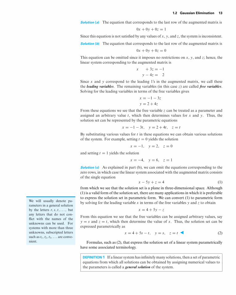
DEFINITION1 If a linear system has infinitely many solutions, then a set of parametricequations from which all solutions can be obtained by assigning numerical values tothe parameters is called a general solution of the system.
14 Chapter 1 Systems of Linear Equations and Matrices
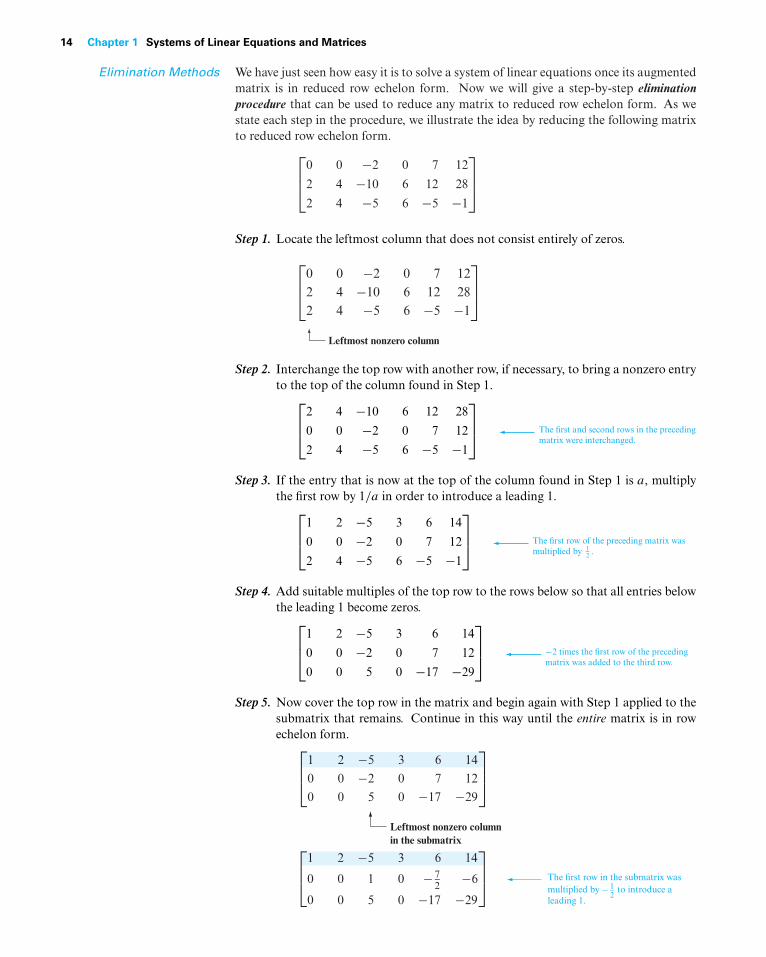
Elimination Methods We have just seen how easy it is to solve a system of linear equations once its augmentedmatrix is in reduced row echelon form. Now we will give a step-by-step eliminationprocedure that can be used to reduce any matrix to reduced row echelon form. As westate each step in the procedure, we illustrate the idea by reducing the following matrixto reduced row echelon form.⎡
⎢⎣0 0 −2 0 7 12
2 4 −10 6 12 28
2 4 −5 6 −5 −1
⎤⎥⎦
Step 1. Locate the leftmost column that does not consist entirely of zeros.
⎡⎢⎣
0 0 2 0 7 122 4 10 6 12 282 4 5 6 5 1
⎤⎥⎦
Leftmost nonzero column
Step 2. Interchange the top row with another row, if necessary, to bring a nonzero entryto the top of the column found in Step 1.⎡
⎢⎣2 4 −10 6 12 28
0 0 −2 0 7 12
2 4 −5 6 −5 −1
⎤⎥⎦ The first and second rows in the preceding
matrix were interchanged.
Step 3. If the entry that is now at the top of the column found in Step 1 is a, multiplythe first row by 1/a in order to introduce a leading 1.⎡
⎢⎣1 2 −5 3 6 14
0 0 −2 0 7 12
2 4 −5 6 −5 −1
⎤⎥⎦ The first row of the preceding matrix was
multiplied by 12 .
Step 4. Add suitable multiples of the top row to the rows below so that all entries belowthe leading 1 become zeros.⎡
⎢⎣1 2 −5 3 6 14
0 0 −2 0 7 12
0 0 5 0 −17 −29
⎤⎥⎦ −2 times the first row of the preceding
matrix was added to the third row.
Step 5. Now cover the top row in the matrix and begin again with Step 1 applied to thesubmatrix that remains. Continue in this way until the entire matrix is in rowechelon form.
⎡⎢⎣
1 2 5 3 6 14
0 0 1 0 72
6
0 0 5 0 17 29
⎤⎥⎦ The first row in the submatrix was
multiplied by 12
to introduce aleading 1.
⎡⎢⎣
1 2 5 3 6 14
0 0 2 0 7 12
0 0 5 0 17 29
⎤⎥⎦
Leftmost nonzero columnin the submatrix
1.2 Gaussian Elimination 15
⎡⎢⎣
1 2 5 3 6 14
0 0 1 0 72
6
0 0 0 0 12
1
⎤⎥⎦ The top row in the submatrix was
covered, and we returned again toStep 1.
Leftmost nonzero columnin the new submatrix
⎡⎢⎣
1 2 5 3 6 14
0 0 1 0 72
6
0 0 0 0 12
1
⎤⎥⎦ –5 times the first row of the submatrix
was added to the second row of thesubmatrix to introduce a zero belowthe leading 1.
⎡⎢⎣
1 2 5 3 6 14
0 0 1 0 72
60 0 0 0 1 2
⎤⎥⎦ The first (and only) row in the new
submatrix was multiplied by 2 tointroduce a leading 1.
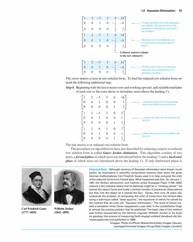
The entire matrix is now in row echelon form. To find the reduced row echelon form weneed the following additional step.
Step 6. Beginning with the last nonzero row and working upward, add suitable multiplesof each row to the rows above to introduce zeros above the leading 1’s.⎡
⎢⎣1 2 −5 3 6 14
0 0 1 0 0 1
0 0 0 0 1 2
⎤⎥⎦ 7
2 times the third row of the precedingmatrix was added to the second row.
⎡⎢⎣1 2 −5 3 0 2
0 0 1 0 0 1
0 0 0 0 1 2
⎤⎥⎦ −6 times the third row was added to the
first row.
⎡⎢⎣1 2 0 3 0 7
0 0 1 0 0 1
0 0 0 0 1 2
⎤⎥⎦ 5 times the second row was added to the
first row.
The last matrix is in reduced row echelon form.The procedure (or algorithm) we have just described for reducing a matrix to reduced
row echelon form is called Gauss–Jordan elimination. This algorithm consists of twoparts, a forward phase in which zeros are introduced below the leading 1’s and a backwardphase in which zeros are introduced above the leading 1’s. If only theforward phase is
Carl Friedrich Gauss(1777–1855)
Wilhelm Jordan(1842–1899)
Historical Note Although versions of Gaussian elimination were known muchearlier, its importance in scientific computation became clear when the greatGerman mathematician Carl Friedrich Gauss used it to help compute the orbitof the asteroid Ceres from limited data. What happened was this: On January 1,1801 the Sicilian astronomer and Catholic priest Giuseppe Piazzi (1746–1826)noticed a dim celestial object that he believed might be a “missing planet.” Henamed the object Ceres and made a limited number of positional observationsbut then lost the object as it neared the Sun. Gauss, then only 24 years old,undertook the problem of computing the orbit of Ceres from the limited datausing a technique called “least squares,” the equations of which he solved bythe method that we now call “Gaussian elimination.” The work of Gauss cre-ated a sensation when Ceres reappeared a year later in the constellation Virgoat almost the precise position that he predicted! The basic idea of the methodwas further popularized by the German engineer Wilhelm Jordan in his bookon geodesy (the science of measuring Earth shapes) entitled Handbuch derVer-messungskunde and published in 1888.
[Images: Photo Inc/Photo Researchers/Getty Images (Gauss);Leemage/Universal Images Group/Getty Images (Jordan)]
16 Chapter 1 Systems of Linear Equations and Matrices
used, then the procedure produces a row echelon form and is called Gaussian elimination.For example, in the preceding computations a row echelon form was obtained at the endof Step 5.
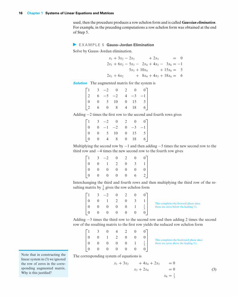
EXAMPLE 5 Gauss–Jordan Elimination
Solve by Gauss–Jordan elimination.
x1 + 3x2 − 2x3 + 2x5 = 0
2x1 + 6x2 − 5x3 − 2x4 + 4x5 − 3x6 = −1
5x3 + 10x4 + 15x6 = 5
2x1 + 6x2 + 8x4 + 4x5 + 18x6 = 6
Solution The augmented matrix for the system is⎡⎢⎢⎢⎣
1 3 −2 0 2 0 0
2 6 −5 −2 4 −3 −1
0 0 5 10 0 15 5
2 6 0 8 4 18 6
⎤⎥⎥⎥⎦
Adding −2 times the first row to the second and fourth rows gives⎡⎢⎢⎢⎣
1 3 −2 0 2 0 0
0 0 −1 −2 0 −3 −1
0 0 5 10 0 15 5
0 0 4 8 0 18 6
⎤⎥⎥⎥⎦
Multiplying the second row by −1 and then adding −5 times the new second row to thethird row and −4 times the new second row to the fourth row gives⎡
⎢⎢⎢⎣1 3 −2 0 2 0 0
0 0 1 2 0 3 1
0 0 0 0 0 0 0
0 0 0 0 0 6 2
⎤⎥⎥⎥⎦
Interchanging the third and fourth rows and then multiplying the third row of the re-sulting matrix by 1
6 gives the row echelon form⎡⎢⎢⎢⎣
1 3 −2 0 2 0 0
0 0 1 2 0 3 1
0 0 0 0 0 1 13
0 0 0 0 0 0 0
⎤⎥⎥⎥⎦ This completes the forward phase since
there are zeros below the leading 1’s.
Adding −3 times the third row to the second row and then adding 2 times the secondrow of the resulting matrix to the first row yields the reduced row echelon form⎡
⎢⎢⎢⎣1 3 0 4 2 0 0
0 0 1 2 0 0 0
0 0 0 0 0 1 13
0 0 0 0 0 0 0
⎤⎥⎥⎥⎦ This completes the backward phase since
there are zeros above the leading 1’s.
The corresponding system of equations isNote that in constructing thelinear system in (3) we ignoredthe row of zeros in the corre-sponding augmented matrix.Why is this justified?
x1 + 3x2 + 4x4 + 2x5 = 0
x3 + 2x4 = 0
x6 = 13
(3)
1.2 Gaussian Elimination 17
Solving for the leading variables, we obtain
x1 = −3x2 − 4x4 − 2x5
x3 = −2x4
x6 = 13
Finally, we express the general solution of the system parametrically by assigning thefree variables x2, x4, and x5 arbitrary values r, s, and t , respectively. This yields
x1 = −3r − 4s − 2t, x2 = r, x3 = −2s, x4 = s, x5 = t, x6 = 13
Homogeneous LinearSystems
A system of linear equations is said to be homogeneous if the constant terms are all zero;that is, the system has the form
a11x1 + a12x2 + · · ·+ a1nxn = 0
a21x1 + a22x2 + · · ·+ a2nxn = 0...
......
...
am1x1 + am2x2 + · · ·+ amnxn = 0
Every homogeneous system of linear equations is consistent because all such systemshave x1 = 0, x2 = 0, . . . , xn = 0 as a solution. This solution is called the trivial solution;if there are other solutions, they are called nontrivial solutions.
Because a homogeneous linear system always has the trivial solution, there are onlytwo possibilities for its solutions:
• The system has only the trivial solution.
• The system has infinitely many solutions in addition to the trivial solution.
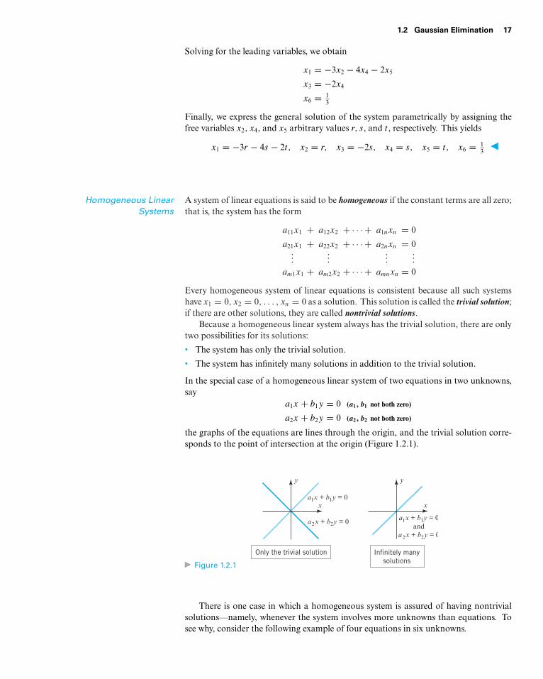
In the special case of a homogeneous linear system of two equations in two unknowns,say
a1x + b1y = 0 (a1, b1 not both zero)
a2x + b2y = 0 (a2, b2 not both zero)
the graphs of the equations are lines through the origin, and the trivial solution corre-sponds to the point of intersection at the origin (Figure 1.2.1).
Figure 1.2.1
x
y
Only the trivial solution
x
y
Infinitely many
solutions
a1x + b1y = 0
a1x + b1y = 0and
a2x + b2y = 0
a2x + b2y = 0
There is one case in which a homogeneous system is assured of having nontrivialsolutions—namely, whenever the system involves more unknowns than equations. Tosee why, consider the following example of four equations in six unknowns.
18 Chapter 1 Systems of Linear Equations and Matrices
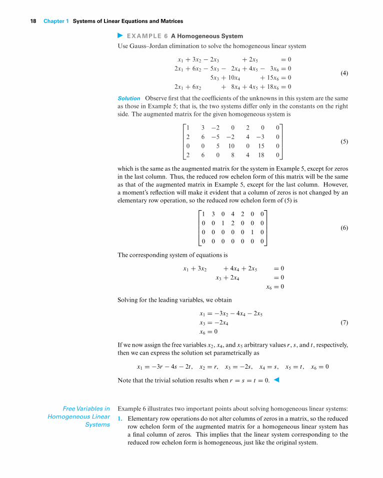
EXAMPLE 6 A Homogeneous System
Use Gauss–Jordan elimination to solve the homogeneous linear system
x1 + 3x2 − 2x3 + 2x5 = 0
2x1 + 6x2 − 5x3 − 2x4 + 4x5 − 3x6 = 0
5x3 + 10x4 + 15x6 = 0
2x1 + 6x2 + 8x4 + 4x5 + 18x6 = 0
(4)
Solution Observe first that the coefficients of the unknowns in this system are the sameas those in Example 5; that is, the two systems differ only in the constants on the rightside. The augmented matrix for the given homogeneous system is⎡
⎢⎢⎢⎣1 3 −2 0 2 0 0
2 6 −5 −2 4 −3 0
0 0 5 10 0 15 02 6 0 8 4 18 0
⎤⎥⎥⎥⎦ (5)
which is the same as the augmented matrix for the system in Example 5, except for zerosin the last column. Thus, the reduced row echelon form of this matrix will be the sameas that of the augmented matrix in Example 5, except for the last column. However,a moment’s reflection will make it evident that a column of zeros is not changed by anelementary row operation, so the reduced row echelon form of (5) is⎡
⎢⎢⎢⎣1 3 0 4 2 0 0
0 0 1 2 0 0 0
0 0 0 0 0 1 0
0 0 0 0 0 0 0
⎤⎥⎥⎥⎦ (6)
The corresponding system of equations is
x1 + 3x2 + 4x4 + 2x5 = 0
x3 + 2x4 = 0
x6 = 0
Solving for the leading variables, we obtain
x1 = −3x2 − 4x4 − 2x5
x3 = −2x4
x6 = 0(7)
If we now assign the free variables x2, x4, and x5 arbitrary values r , s, and t , respectively,then we can express the solution set parametrically as
x1 = −3r − 4s − 2t, x2 = r, x3 = −2s, x4 = s, x5 = t, x6 = 0
Note that the trivial solution results when r = s = t = 0.
FreeVariables inHomogeneous Linear
Systems
Example 6 illustrates two important points about solving homogeneous linear systems:
1. Elementary row operations do not alter columns of zeros in a matrix, so the reducedrow echelon form of the augmented matrix for a homogeneous linear system hasa final column of zeros. This implies that the linear system corresponding to thereduced row echelon form is homogeneous, just like the original system.
1.2 Gaussian Elimination 19
2. When we constructed the homogeneous linear system corresponding to augmentedmatrix (6), we ignored the row of zeros because the corresponding equation
0x1 + 0x2 + 0x3 + 0x4 + 0x5 + 0x6 = 0
does not impose any conditions on the unknowns. Thus, depending on whether ornot the reduced row echelon form of the augmented matrix for a homogeneous linearsystem has any rows of zero, the linear system corresponding to that reduced rowechelon form will either have the same number of equations as the original systemor it will have fewer.
Now consider a general homogeneous linear system with n unknowns, and supposethat the reduced row echelon form of the augmented matrix has r nonzero rows. Sinceeach nonzero row has a leading 1, and since each leading 1 corresponds to a leadingvariable, the homogeneous system corresponding to the reduced row echelon form ofthe augmented matrix must have r leading variables and n − r free variables. Thus, thissystem is of the form
xk1 +∑( ) = 0
xk2 +∑( ) = 0
. . ....
xkr+∑
( ) = 0
(8)
where in each equation the expression∑
( ) denotes a sum that involves the free variables,if any [see (7), for example]. In summary, we have the following result.
THEOREM 1.2.1 FreeVariableTheorem for Homogeneous Systems
If a homogeneous linear system has n unknowns, and if the reduced row echelon formof its augmented matrix has r nonzero rows, then the system has n − r free variables.
Theorem 1.2.1 has an important implication for homogeneous linear systems withNote that Theorem 1.2.2 ap-plies only to homogeneoussystems—a nonhomogeneoussystem with more unknownsthan equations need not beconsistent. However, we willprove later that if a nonho-mogeneous system with moreunknowns then equations isconsistent, then it has in-finitely many solutions.
more unknowns than equations. Specifically, if a homogeneous linear system has m
equations in n unknowns, and if m < n, then it must also be true that r < n (why?).This being the case, the theorem implies that there is at least one free variable, and thisimplies that the system has infinitely many solutions. Thus, we have the following result.
THEOREM 1.2.2 A homogeneous linear system with more unknowns than equations hasinfinitely many solutions.
In retrospect, we could have anticipated that the homogeneous system in Example 6would have infinitely many solutions since it has four equations in six unknowns.
Gaussian Elimination andBack-Substitution
For small linear systems that are solved by hand (such as most of those in this text),Gauss–Jordan elimination (reduction to reduced row echelon form) is a good procedureto use. However, for large linear systems that require a computer solution, it is generallymore efficient to use Gaussian elimination (reduction to row echelon form) followed bya technique known as back-substitution to complete the process of solving the system.The next example illustrates this technique.
20 Chapter 1 Systems of Linear Equations and Matrices
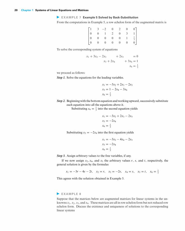
EXAMPLE 7 Example 5 Solved by Back-Substitution
From the computations in Example 5, a row echelon form of the augmented matrix is⎡⎢⎢⎢⎣
1 3 −2 0 2 0 0
0 0 1 2 0 3 1
0 0 0 0 0 1 13
0 0 0 0 0 0 0
⎤⎥⎥⎥⎦
To solve the corresponding system of equations
x1 + 3x2 − 2x3 + 2x5 = 0
x3 + 2x4 + 3x6 = 1
x6 = 13
we proceed as follows:
Step 1. Solve the equations for the leading variables.
x1 = −3x2 + 2x3 − 2x5
x3 = 1 − 2x4 − 3x6
x6 = 13
Step 2. Beginning with the bottom equation and working upward, successively substituteeach equation into all the equations above it.
Substituting x6 = 13 into the second equation yields
x1 = −3x2 + 2x3 − 2x5
x3 = −2x4
x6 = 13
Substituting x3 = −2x4 into the first equation yields
x1 = −3x2 − 4x4 − 2x5
x3 = −2x4
x6 = 13
Step 3. Assign arbitrary values to the free variables, if any.
If we now assign x2, x4, and x5 the arbitrary values r , s, and t , respectively, thegeneral solution is given by the formulas
x1 = −3r − 4s − 2t, x2 = r, x3 = −2s, x4 = s, x5 = t, x6 = 13
This agrees with the solution obtained in Example 5.
EXAMPLE 8
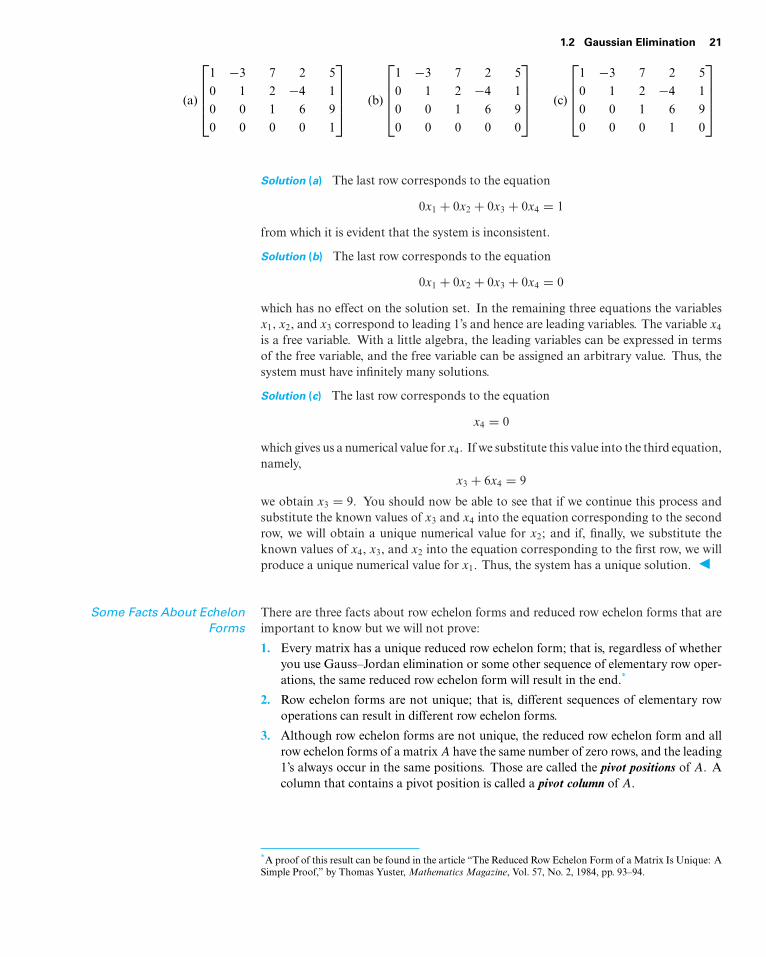
Suppose that the matrices below are augmented matrices for linear systems in the un-knowns x1, x2, x3, and x4. These matrices are all in row echelon form but not reduced rowechelon form. Discuss the existence and uniqueness of solutions to the correspondinglinear systems
1.2 Gaussian Elimination 21
(a)
⎡⎢⎢⎢⎣
1 −3 7 2 5
0 1 2 −4 1
0 0 1 6 9
0 0 0 0 1
⎤⎥⎥⎥⎦ (b)
⎡⎢⎢⎢⎣
1 −3 7 2 5
0 1 2 −4 1
0 0 1 6 9
0 0 0 0 0
⎤⎥⎥⎥⎦ (c)
⎡⎢⎢⎢⎣
1 −3 7 2 5
0 1 2 −4 1
0 0 1 6 9
0 0 0 1 0
⎤⎥⎥⎥⎦
Solution (a) The last row corresponds to the equation
0x1 + 0x2 + 0x3 + 0x4 = 1
from which it is evident that the system is inconsistent.
Solution (b) The last row corresponds to the equation
0x1 + 0x2 + 0x3 + 0x4 = 0
which has no effect on the solution set. In the remaining three equations the variablesx1, x2, and x3 correspond to leading 1’s and hence are leading variables. The variable x4
is a free variable. With a little algebra, the leading variables can be expressed in termsof the free variable, and the free variable can be assigned an arbitrary value. Thus, thesystem must have infinitely many solutions.
Solution (c) The last row corresponds to the equation
x4 = 0
which gives us a numerical value for x4. If we substitute this value into the third equation,namely,
x3 + 6x4 = 9
we obtain x3 = 9. You should now be able to see that if we continue this process andsubstitute the known values of x3 and x4 into the equation corresponding to the secondrow, we will obtain a unique numerical value for x2; and if, finally, we substitute theknown values of x4, x3, and x2 into the equation corresponding to the first row, we willproduce a unique numerical value for x1. Thus, the system has a unique solution.
Some Facts About EchelonForms
There are three facts about row echelon forms and reduced row echelon forms that areimportant to know but we will not prove:
1. Every matrix has a unique reduced row echelon form; that is, regardless of whetheryou use Gauss–Jordan elimination or some other sequence of elementary row oper-ations, the same reduced row echelon form will result in the end.*
2. Row echelon forms are not unique; that is, different sequences of elementary rowoperations can result in different row echelon forms.
3. Although row echelon forms are not unique, the reduced row echelon form and allrow echelon forms of a matrix A have the same number of zero rows, and the leading1’s always occur in the same positions. Those are called the pivot positions of A. Acolumn that contains a pivot position is called a pivot column of A.
*A proof of this result can be found in the article “The Reduced Row Echelon Form of a Matrix Is Unique: ASimple Proof,” by Thomas Yuster, Mathematics Magazine, Vol. 57, No. 2, 1984, pp. 93–94.
22 Chapter 1 Systems of Linear Equations and Matrices
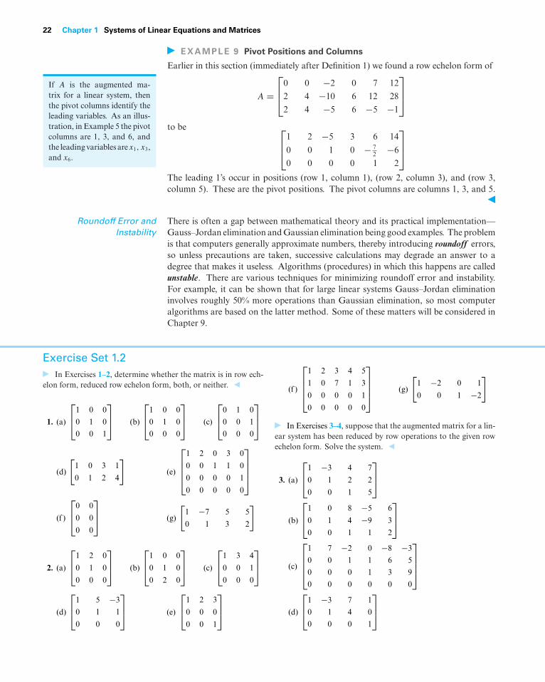
EXAMPLE 9 Pivot Positions and Columns
Earlier in this section (immediately after Definition 1) we found a row echelon form of
A =⎡⎢⎣0 0 −2 0 7 12
2 4 −10 6 12 28
2 4 −5 6 −5 −1
⎤⎥⎦
to be ⎡⎢⎣1 2 −5 3 6 14
0 0 1 0 − 72 −6
0 0 0 0 1 2
⎤⎥⎦
The leading 1’s occur in positions (row 1, column 1), (row 2, column 3), and (row 3,column 5). These are the pivot positions. The pivot columns are columns 1, 3, and 5.
If A is the augmented ma-trix for a linear system, thenthe pivot columns identify theleading variables. As an illus-tration, in Example 5 the pivotcolumns are 1, 3, and 6, andthe leading variables arex1, x3,and x6.
Roundoff Error andInstability
There is often a gap between mathematical theory and its practical implementation—Gauss–Jordan elimination and Gaussian elimination being good examples. The problemis that computers generally approximate numbers, thereby introducing roundoff errors,so unless precautions are taken, successive calculations may degrade an answer to adegree that makes it useless. Algorithms (procedures) in which this happens are calledunstable. There are various techniques for minimizing roundoff error and instability.For example, it can be shown that for large linear systems Gauss–Jordan eliminationinvolves roughly 50% more operations than Gaussian elimination, so most computeralgorithms are based on the latter method. Some of these matters will be considered inChapter 9.
Exercise Set 1.2
In Exercises 1–2, determine whether the matrix is in row ech-elon form, reduced row echelon form, both, or neither.
1. (a)
⎡⎢⎣1 0 0
0 1 0
0 0 1
⎤⎥⎦ (b)
⎡⎢⎣1 0 0
0 1 0
0 0 0
⎤⎥⎦ (c)
⎡⎢⎣0 1 0
0 0 1
0 0 0
⎤⎥⎦
(d)
[1 0 3 1
0 1 2 4
](e)
⎡⎢⎢⎢⎣
1 2 0 3 0
0 0 1 1 0
0 0 0 0 1
0 0 0 0 0
⎤⎥⎥⎥⎦
(f )
⎡⎢⎣0 0
0 0
0 0
⎤⎥⎦ (g)
[1 −7 5 5
0 1 3 2
]
2. (a)
⎡⎢⎣1 2 0
0 1 0
0 0 0
⎤⎥⎦ (b)
⎡⎢⎣1 0 0
0 1 0
0 2 0
⎤⎥⎦ (c)
⎡⎢⎣1 3 4
0 0 1
0 0 0
⎤⎥⎦
(d)
⎡⎢⎣1 5 −3
0 1 1
0 0 0
⎤⎥⎦ (e)
⎡⎢⎣1 2 3
0 0 0
0 0 1
⎤⎥⎦
(f )
⎡⎢⎢⎢⎣
1 2 3 4 5
1 0 7 1 3
0 0 0 0 1
0 0 0 0 0
⎤⎥⎥⎥⎦ (g)
[1 −2 0 1
0 0 1 −2
]
In Exercises 3–4, suppose that the augmented matrix for a lin-ear system has been reduced by row operations to the given rowechelon form. Solve the system.
3. (a)
⎡⎢⎣1 −3 4 7
0 1 2 2
0 0 1 5
⎤⎥⎦
(b)
⎡⎢⎣1 0 8 −5 6
0 1 4 −9 3
0 0 1 1 2
⎤⎥⎦
(c)
⎡⎢⎢⎢⎣
1 7 −2 0 −8 −3
0 0 1 1 6 5
0 0 0 1 3 9
0 0 0 0 0 0
⎤⎥⎥⎥⎦
(d)
⎡⎢⎣1 −3 7 1
0 1 4 0
0 0 0 1
⎤⎥⎦
1.2 Gaussian Elimination 23
4. (a)
⎡⎢⎣1 0 0 −3
0 1 0 0
0 0 1 7
⎤⎥⎦
(b)
⎡⎢⎣1 0 0 −7 8
0 1 0 3 2
0 0 1 1 −5
⎤⎥⎦
(c)
⎡⎢⎢⎢⎣
1 −6 0 0 3 −2
0 0 1 0 4 7
0 0 0 1 5 8
0 0 0 0 0 0
⎤⎥⎥⎥⎦
(d)
⎡⎢⎣1 −3 0 0
0 0 1 0
0 0 0 1
⎤⎥⎦
In Exercises 5–8, solve the linear system by Gaussian elimi-nation.
5. x1 + x2 + 2x3 = 8
−x1 − 2x2 + 3x3 = 1
3x1 − 7x2 + 4x3 = 10
6. 2x1 + 2x2 + 2x3 = 0
−2x1 + 5x2 + 2x3 = 1
8x1 + x2 + 4x3 = −1
7. x − y + 2z − w = −1
2x + y − 2z − 2w = −2
−x + 2y − 4z + w = 1
3x − 3w = −3
8. − 2b + 3c = 1
3a + 6b − 3c = −2
6a + 6b + 3c = 5
In Exercises 9–12, solve the linear system by Gauss–Jordanelimination.
9. Exercise 5 10. Exercise 6
11. Exercise 7 12. Exercise 8
In Exercises 13–14, determine whether the homogeneous sys-tem has nontrivial solutions by inspection (without pencil andpaper).
13. 2x1 − 3x2 + 4x3 − x4 = 0
7x1 + x2 − 8x3 + 9x4 = 0
2x1 + 8x2 + x3 − x4 = 0
14. x1 + 3x2 − x3 = 0
x2 − 8x3 = 0
4x3 = 0
In Exercises 15–22, solve the given linear system by anymethod.
15. 2x1 + x2 + 3x3 = 0
x1 + 2x2 = 0
x2 + x3 = 0
16. 2x − y − 3z = 0
−x + 2y − 3z = 0
x + y + 4z = 0
17. 3x1 + x2 + x3 + x4 = 0
5x1 − x2 + x3 − x4 = 0
18. v + 3w − 2x = 0
2u + v − 4w + 3x = 0
2u + 3v + 2w − x = 0
−4u − 3v + 5w − 4x = 0
19. 2x + 2y + 4z = 0
w − y − 3z = 0
2w + 3x + y + z = 0
−2w + x + 3y − 2z = 0
20. x1 + 3x2 + x4 = 0
x1 + 4x2 + 2x3 = 0
− 2x2 − 2x3 − x4 = 0
2x1 − 4x2 + x3 + x4 = 0
x1 − 2x2 − x3 + x4 = 0
21. 2I1 − I2 + 3I3 + 4I4 = 9
I1 − 2I3 + 7I4 = 11
3I1 − 3I2 + I3 + 5I4 = 8
2I1 + I2 + 4I3 + 4I4 = 10
22. Z3 + Z4 + Z5 = 0
−Z1 − Z2 + 2Z3 − 3Z4 + Z5 = 0
Z1 + Z2 − 2Z3 − Z5 = 0
2Z1 + 2Z2 − Z3 + Z5 = 0
In each part of Exercises 23–24, the augmented matrix for alinear system is given in which the asterisk represents an unspec-ified real number. Determine whether the system is consistent,and if so whether the solution is unique. Answer “inconclusive” ifthere is not enough information to make a decision.
23. (a)
⎡⎣1 ∗ ∗ ∗
0 1 ∗ ∗0 0 1 ∗
⎤⎦ (b)
⎡⎣1 ∗ ∗ ∗
0 1 ∗ ∗0 0 0 0
⎤⎦
(c)
⎡⎣1 ∗ ∗ ∗
0 1 ∗ ∗0 0 0 1
⎤⎦ (d)
⎡⎣1 ∗ ∗ ∗
0 0 ∗ 00 0 1 ∗
⎤⎦
24. (a)
⎡⎣1 ∗ ∗ ∗
0 1 ∗ ∗0 0 1 1
⎤⎦ (b)
⎡⎣1 0 0 ∗∗ 1 0 ∗∗ ∗ 1 ∗
⎤⎦
(c)
⎡⎣1 0 0 0
1 0 0 11 ∗ ∗ ∗
⎤⎦ (d)
⎡⎣1 ∗ ∗ ∗
1 0 0 11 0 0 1
⎤⎦
In Exercises 25–26, determine the values of a for which thesystem has no solutions, exactly one solution, or infinitely manysolutions.
25. x + 2y − 3z = 4
3x − y + 5z = 2
4x + y + (a2 − 14)z = a + 2
24 Chapter 1 Systems of Linear Equations and Matrices
26. x + 2y + z = 2
2x − 2y + 3z = 1
x + 2y − (a2 − 3)z = a
In Exercises 27–28, what condition, if any, must a, b, and c
satisfy for the linear system to be consistent?
27. x + 3y − z = a
x + y + 2z = b
2y − 3z = c
28. x + 3y + z = a
−x − 2y + z = b
3x + 7y − z = c
In Exercises 29–30, solve the following systems, where a, b,and c are constants.
29. 2x + y = a
3x + 6y = b
30. x1 + x2 + x3 = a
2x1 + 2x3 = b
3x2 + 3x3 = c
31. Find two different row echelon forms of[1 3
2 7
]
This exercise shows that a matrix can have multiple row eche-lon forms.
32. Reduce ⎡⎢⎣2 1 3
0 −2 −29
3 4 5
⎤⎥⎦
to reduced row echelon form without introducing fractions atany intermediate stage.
33. Show that the following nonlinear system has 18 solutions if0 ≤ α ≤ 2π , 0 ≤ β ≤ 2π , and 0 ≤ γ ≤ 2π .
sin α + 2 cos β + 3 tan γ = 0
2 sin α + 5 cos β + 3 tan γ = 0
− sin α − 5 cos β + 5 tan γ = 0
[Hint: Begin by making the substitutions x = sin α,y = cos β, and z = tan γ .]
34. Solve the following system of nonlinear equations for the un-known angles α, β, and γ , where 0 ≤ α ≤ 2π , 0 ≤ β ≤ 2π ,and 0 ≤ γ < π .
2 sin α − cos β + 3 tan γ = 3
4 sin α + 2 cos β − 2 tan γ = 2
6 sin α − 3 cos β + tan γ = 9
35. Solve the following system of nonlinear equations for x, y,
and z.
x2 + y2 + z2 = 6
x2 − y2 + 2z2 = 2
2x2 + y2 − z2 = 3
[Hint: Begin by making the substitutions X = x2, Y = y2,
Z = z2.]
36. Solve the following system for x, y, and z.
1
x+ 2
y− 4
z= 1
2
x+ 3
y+ 8
z= 0
− 1
x+ 9
y+ 10
z= 5
37. Find the coefficients a, b, c, and d so that the curve shownin the accompanying figure is the graph of the equationy = ax3 + bx2 + cx + d.
y
x
–2 6
–20
20(0, 10) (1, 7)
(3, –11) (4, –14)
Figure Ex-37
38. Find the coefficients a, b, c, and d so that the circle shown inthe accompanying figure is given by the equationax2 + ay2 + bx + cy + d = 0.
y
x
(–2, 7)
(4, –3)
(–4, 5)
Figure Ex-38
39. If the linear system
a1x + b1y + c1z = 0
a2x − b2y + c2z = 0
a3x + b3y − c3z = 0
has only the trivial solution, what can be said about the solu-tions of the following system?
a1x + b1y + c1z = 3
a2x − b2y + c2z = 7
a3x + b3y − c3z = 11
40. (a) If A is a matrix with three rows and five columns, thenwhat is the maximum possible number of leading 1’s in itsreduced row echelon form?
(b) If B is a matrix with three rows and six columns, thenwhat is the maximum possible number of parameters inthe general solution of the linear system with augmentedmatrix B?
(c) If C is a matrix with five rows and three columns, thenwhat is the minimum possible number of rows of zeros inany row echelon form of C?
1.3 Matrices and Matrix Operations 25
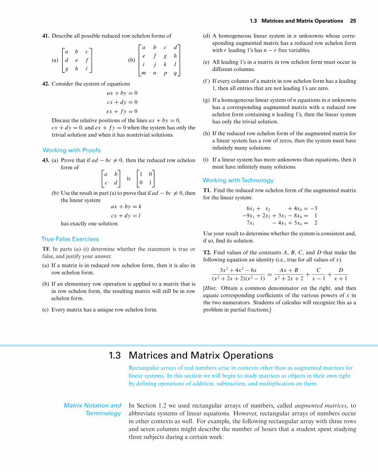
41. Describe all possible reduced row echelon forms of
(a)
⎡⎢⎣a b c
d e f
g h i
⎤⎥⎦ (b)
⎡⎢⎢⎢⎣
a b c d
e f g h
i j k l
m n p q
⎤⎥⎥⎥⎦
42. Consider the system of equations
ax + by = 0
cx + dy = 0
ex + fy = 0
Discuss the relative positions of the lines ax + by = 0,cx + dy = 0, and ex + fy = 0 when the system has only thetrivial solution and when it has nontrivial solutions.
Working with Proofs
43. (a) Prove that if ad − bc �= 0, then the reduced row echelonform of [
a b
c d
]is
[1 0
0 1
]
(b) Use the result in part (a) to prove that if ad − bc �= 0, thenthe linear system
ax + by = k
cx + dy = l
has exactly one solution.
True-False Exercises
TF. In parts (a)–(i) determine whether the statement is true orfalse, and justify your answer.
(a) If a matrix is in reduced row echelon form, then it is also inrow echelon form.
(b) If an elementary row operation is applied to a matrix that isin row echelon form, the resulting matrix will still be in rowechelon form.
(c) Every matrix has a unique row echelon form.
(d) A homogeneous linear system in n unknowns whose corre-sponding augmented matrix has a reduced row echelon formwith r leading 1’s has n − r free variables.
(e) All leading 1’s in a matrix in row echelon form must occur indifferent columns.
(f ) If every column of a matrix in row echelon form has a leading1, then all entries that are not leading 1’s are zero.
(g) If a homogeneous linear system of n equations in n unknownshas a corresponding augmented matrix with a reduced rowechelon form containing n leading 1’s, then the linear systemhas only the trivial solution.
(h) If the reduced row echelon form of the augmented matrix fora linear system has a row of zeros, then the system must haveinfinitely many solutions.
(i) If a linear system has more unknowns than equations, then itmust have infinitely many solutions.
Working withTechnology
T1. Find the reduced row echelon form of the augmented matrixfor the linear system:
6x1 + x2 + 4x4 = −3−9x1 + 2x2 + 3x3 − 8x4 = 1
7x1 − 4x3 + 5x4 = 2
Use your result to determine whether the system is consistent and,if so, find its solution.
T2. Find values of the constants A, B, C, and D that make thefollowing equation an identity (i.e., true for all values of x).
3x3 + 4x2 − 6x
(x2 + 2x + 2)(x2 − 1)= Ax + B
x2 + 2x + 2+ C
x − 1+ D
x + 1
[Hint: Obtain a common denominator on the right, and thenequate corresponding coefficients of the various powers of x inthe two numerators. Students of calculus will recognize this as aproblem in partial fractions.]
1.3 Matrices and Matrix OperationsRectangular arrays of real numbers arise in contexts other than as augmented matrices forlinear systems. In this section we will begin to study matrices as objects in their own rightby defining operations of addition, subtraction, and multiplication on them.
Matrix Notation andTerminology
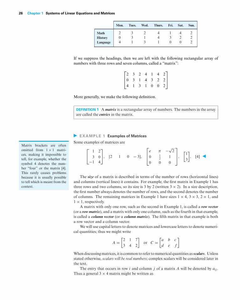
In Section 1.2 we used rectangular arrays of numbers, called augmented matrices, toabbreviate systems of linear equations. However, rectangular arrays of numbers occurin other contexts as well. For example, the following rectangular array with three rowsand seven columns might describe the number of hours that a student spent studyingthree subjects during a certain week:
26 Chapter 1 Systems of Linear Equations and Matrices
204
331
213
441
130
420
222
Mon.
MathHistoryLanguage
Tues. Wed. Thurs. Fri. Sat. Sun.
If we suppress the headings, then we are left with the following rectangular array ofnumbers with three rows and seven columns, called a “matrix”:
⎡⎢⎣2 3 2 4 1 4 2
0 3 1 4 3 2 2
4 1 3 1 0 0 2
⎤⎥⎦
More generally, we make the following definition.
DEFINITION 1 A matrix is a rectangular array of numbers. The numbers in the arrayare called the entries in the matrix.
EXAMPLE 1 Examples of Matrices
Some examples of matrices areMatrix brackets are oftenomitted from 1 × 1 matri-ces, making it impossible totell, for example, whether thesymbol 4 denotes the num-ber “four” or the matrix [4].This rarely causes problemsbecause it is usually possibleto tell which is meant from thecontext.
⎡⎣ 1 2
3 0−1 4
⎤⎦, [2 1 0 − 3],
⎡⎢⎣e π −√
2
0 12 1
0 0 0
⎤⎥⎦,
[1
3
], [4]
The size of a matrix is described in terms of the number of rows (horizontal lines)and columns (vertical lines) it contains. For example, the first matrix in Example 1 hasthree rows and two columns, so its size is 3 by 2 (written 3 × 2). In a size description,the first number always denotes the number of rows, and the second denotes the numberof columns. The remaining matrices in Example 1 have sizes 1 × 4, 3 × 3, 2 × 1, and1 × 1, respectively.
A matrix with only one row, such as the second in Example 1, is called a row vector(or a row matrix), and a matrix with only one column, such as the fourth in that example,is called a column vector (or a column matrix). The fifth matrix in that example is botha row vector and a column vector.
We will use capital letters to denote matrices and lowercase letters to denote numeri-cal quantities; thus we might write
A =[
2 1 7
3 4 2
]or C =
[a b c
d e f
]When discussing matrices, it is common to refer to numerical quantities as scalars. Unlessstated otherwise, scalars will be real numbers; complex scalars will be considered later inthe text.
The entry that occurs in row i and column j of a matrix A will be denoted by aij .Thus a general 3 × 4 matrix might be written as
1.3 Matrices and Matrix Operations 27
A =⎡⎢⎣a11 a12 a13 a14
a21 a22 a23 a24
a31 a32 a33 a34
⎤⎥⎦
and a general m × n matrix as
A =
⎡⎢⎢⎢⎣
a11 a12 · · · a1n
a21 a22 · · · a2n...
......
am1 am2 · · · amn
⎤⎥⎥⎥⎦ (1)
When a compact notation is desired, the preceding matrix can be written asA matrix with n rows and n
columns is said to be a squarematrix of order n.
[aij ]m×n or [aij ]the first notation being used when it is important in the discussion to know the size,and the second when the size need not be emphasized. Usually, we will match the letterdenoting a matrix with the letter denoting its entries; thus, for a matrix B we wouldgenerally use bij for the entry in row i and column j , and for a matrix C we would usethe notation cij .
The entry in row i and column j of a matrix A is also commonly denoted by thesymbol (A)ij . Thus, for matrix (1) above, we have
(A)ij = aij
and for the matrix
A =[
2 −3
7 0
]we have (A)11 = 2, (A)12 = −3, (A)21 = 7, and (A)22 = 0.
Row and column vectors are of special importance, and it is common practice todenote them by boldface lowercase letters rather than capital letters. For such matrices,double subscripting of the entries is unnecessary. Thus a general 1 × n row vector a anda general m × 1 column vector b would be written as
a = [a1 a2 · · · an] and b =
⎡⎢⎢⎢⎣
b1
b2...
bm
⎤⎥⎥⎥⎦
A matrix A with n rows and n columns is called a square matrix of order n, and theshaded entries a11, a22, . . . , ann in (2) are said to be on the main diagonal of A.
⎡⎢⎢⎢⎣
a11 a12 · · · a1n
a21 a22 · · · a2n...
......
an1 an2 · · · ann
⎤⎥⎥⎥⎦ (2)
Operations on Matrices So far, we have used matrices to abbreviate the work in solving systems of linear equa-tions. For other applications, however, it is desirable to develop an “arithmetic of ma-trices” in which matrices can be added, subtracted, and multiplied in a useful way. Theremainder of this section will be devoted to developing this arithmetic.
DEFINITION 2 Two matrices are defined to be equal if they have the same size andtheir corresponding entries are equal.
28 Chapter 1 Systems of Linear Equations and Matrices
EXAMPLE 2 Equality of Matrices
Consider the matricesThe equality of two matrices
A = [aij ] and B = [bij ]of the same size can be ex-pressed either by writing
(A)ij = (B)ij
or by writing
aij = bij
where it is understood that theequalities hold for all values ofi and j .
A =[
2 1
3 x
], B =
[2 1
3 5
], C =
[2 1 0
3 4 0
]If x = 5, then A = B, but for all other values of x the matrices A and B are not equal,since not all of their corresponding entries are equal. There is no value of x for whichA = C since A and C have different sizes.
DEFINITION 3 If A and B are matrices of the same size, then the sum A + B is thematrix obtained by adding the entries of B to the corresponding entries of A, andthe difference A − B is the matrix obtained by subtracting the entries of B from thecorresponding entries of A. Matrices of different sizes cannot be added or subtracted.
In matrix notation, if A = [aij ] and B = [bij ] have the same size, then
(A + B)ij = (A)ij + (B)ij = aij + bij and (A − B)ij = (A)ij − (B)ij = aij − bij
EXAMPLE 3 Addition and Subtraction
Consider the matrices
A =⎡⎢⎣ 2 1 0 3−1 0 2 4
4 −2 7 0
⎤⎥⎦, B =
⎡⎢⎣−4 3 5 1
2 2 0 −13 2 −4 5
⎤⎥⎦, C =
[1 12 2
]
Then
A + B =⎡⎢⎣−2 4 5 4
1 2 2 37 0 3 5
⎤⎥⎦ and A − B =
⎡⎢⎣ 6 −2 −5 2−3 −2 2 5
1 −4 11 −5
⎤⎥⎦
The expressions A + C, B + C, A − C, and B − C are undefined.
DEFINITION 4 If A is any matrix and c is any scalar, then the product cA is the matrixobtained by multiplying each entry of the matrix A by c. The matrix cA is said to bea scalar multiple of A.
In matrix notation, if A = [aij ], then
(cA)ij = c(A)ij = caij
EXAMPLE 4 Scalar Multiples
For the matrices
A =[
2 3 41 3 1
], B =
[0 2 7
−1 3 −5
], C =
[9 −6 33 0 12
]we have
2A =[
4 6 82 6 2
], (−1)B =
[0 −2 −71 −3 5
], 1
3C =[
3 −2 11 0 4
]It is common practice to denote (−1)B by −B.
1.3 Matrices and Matrix Operations 29
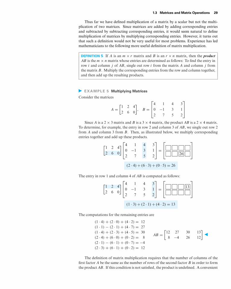
Thus far we have defined multiplication of a matrix by a scalar but not the multi-plication of two matrices. Since matrices are added by adding corresponding entriesand subtracted by subtracting corresponding entries, it would seem natural to definemultiplication of matrices by multiplying corresponding entries. However, it turns outthat such a definition would not be very useful for most problems. Experience has ledmathematicians to the following more useful definition of matrix multiplication.
DEFINITION 5 If A is an m × r matrix and B is an r × n matrix, then the productAB is the m × n matrix whose entries are determined as follows: To find the entry inrow i and column j of AB, single out row i from the matrix A and column j fromthe matrix B. Multiply the corresponding entries from the row and column together,and then add up the resulting products.
EXAMPLE 5 Multiplying Matrices
Consider the matrices
A =[
1 2 4
2 6 0
], B =
⎡⎢⎣4 1 4 3
0 −1 3 1
2 7 5 2
⎤⎥⎦
Since A is a 2 × 3 matrix and B is a 3 × 4 matrix, the product AB is a 2 × 4 matrix.To determine, for example, the entry in row 2 and column 3 of AB, we single out row 2from A and column 3 from B. Then, as illustrated below, we multiply correspondingentries together and add up these products.
[1 2 42 6 0
]⎡⎢⎣4 1 4 30 1 3 12 7 5 2
⎤⎥⎦ =
⎡⎢⎣
26
⎤⎥⎦
(2 · 4) + (6 · 3) + (0 · 5) = 26
The entry in row 1 and column 4 of AB is computed as follows:
[1 2 42 6 0
]⎡⎢⎣4 1 4 30 1 3 12 7 5 2
⎤⎥⎦ =
⎡⎢⎣ 13
⎤⎥⎦
(1 · 3) + (2 · 1) + (4 · 2) = 13
The computations for the remaining entries are
(1 · 4) + (2 · 0) + (4 · 2) = 12(1 · 1) − (2 · 1) + (4 · 7) = 27(1 · 4) + (2 · 3) + (4 · 5) = 30(2 · 4) + (6 · 0) + (0 · 2) = 8(2 · 1) − (6 · 1) + (0 · 7) = −4(2 · 3) + (6 · 1) + (0 · 2) = 12
AB =[
12 27 30 138 −4 26 12
]
The definition of matrix multiplication requires that the number of columns of thefirst factor A be the same as the number of rows of the second factor B in order to formthe product AB. If this condition is not satisfied, the product is undefined. A convenient
30 Chapter 1 Systems of Linear Equations and Matrices
way to determine whether a product of two matrices is defined is to write down the sizeof the first factor and, to the right of it, write down the size of the second factor. If, as in(3), the inside numbers are the same, then the product is defined. The outside numbersthen give the size of the product.
Am × r
Inside
Outside
Br × n =
ABm × n
(3)
EXAMPLE 6 DeterminingWhether a Product Is Defined
Suppose that A, B, and C are matrices with the following sizes:
A B C
3 × 4 4 × 7 7 × 3
Then by (3), AB is defined and is a 3 × 7 matrix; BC is defined and is a 4 × 3 matrix; andCA is defined and is a 7 × 4 matrix. The products AC, CB, and BA are all undefined.
In general, if A = [aij ] is an m × r matrix and B = [bij ] is an r × n matrix, then, asillustrated by the shading in the following display,
AB =
⎡⎢⎢⎢⎢⎢⎢⎢⎢⎣
a11 a12 · · · a1r
a21 a22 · · · a2r...
......
ai1 ai2 · · · air...
......
am1 am2 · · · amr
⎤⎥⎥⎥⎥⎥⎥⎥⎥⎦
⎡⎢⎢⎢⎣
b11 b12 · · · b1 j · · · b1n
b21 b22 · · · b2 j · · · b2n...
......
...
br1 br2 · · · br j · · · brn
⎤⎥⎥⎥⎦ (4)
the entry (AB)ij in row i and column j of AB is given by
(AB)ij = ai1b1j + ai2b2j + ai3b3j + · · · + airbrj (5)
Formula (5) is called the row-column rule for matrix multiplication.
Partitioned Matrices A matrix can be subdivided or partitioned into smaller matrices by inserting horizontaland vertical rules between selected rows and columns. For example, the following arethree possible partitions of a general 3 × 4 matrix A—the first is a partition of A into
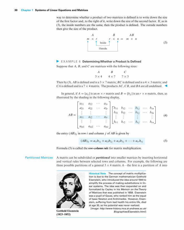
Gotthold Eisenstein(1823–1852)
Historical Note The concept of matrix multiplica-tion is due to the German mathematician GottholdEisenstein, who introduced the idea around 1844 tosimplify the process of making substitutions in lin-ear systems. The idea was then expanded on andformalized by Cayley in his Memoir on the Theoryof Matrices that was published in 1858. Eisensteinwas a pupil of Gauss, who ranked him as the equalof Isaac Newton and Archimedes. However, Eisen-stein, suffering from bad health his entire life, diedat age 30, so his potential was never realized.[Image: http://www-history.mcs.st-andrews.ac.uk/
Biographies/Eisenstein.html]
1.3 Matrices and Matrix Operations 31
four submatrices A11, A12, A21, and A22; the second is a partition of A into its row vectorsr1, r2, and r3; and the third is a partition of A into its column vectors c1, c2, c3, and c4:
A =⎡⎢⎣a11 a12 a13 a14
a21 a22 a23 a24
a31 a32 a33 a34
⎤⎥⎦ =
[A11 A12
A21 A22
]
A =⎡⎢⎣a11 a12 a13 a14
a21 a22 a23 a24
a31 a32 a33 a34
⎤⎥⎦ =
⎡⎢⎣r1
r2
r3
⎤⎥⎦
A =⎡⎢⎣a11 a12 a13 a14
a21 a22 a23 a24
a31 a32 a33 a34
⎤⎥⎦ = [c1 c2 c3 c4]
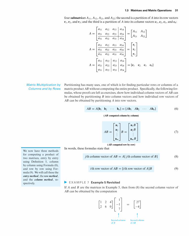
Matrix Multiplication byColumns and by Rows
Partitioning has many uses, one of which is for finding particular rows or columns of amatrix product AB without computing the entire product. Specifically, the following for-mulas, whose proofs are left as exercises, show how individual column vectors of AB canbe obtained by partitioning B into column vectors and how individual row vectors ofAB can be obtained by partitioning A into row vectors.
AB = A[b1 b2 · · · bn] = [Ab1 Ab2 · · · Abn] (6)
(AB computed column by column)
AB =
⎡⎢⎢⎢⎣
a1
a2...
am
⎤⎥⎥⎥⎦B =
⎡⎢⎢⎢⎣
a1B
a2B...
amB
⎤⎥⎥⎥⎦ (7)
(AB computed row by row)
In words, these formulas state thatWe now have three methodsfor computing a product oftwo matrices, entry by entryusing Definition 5, columnby column using Formula (8),and row by row using For-mula (9). We will call these theentry method , the row method ,and the column method , re-spectively.
j th column vector of AB = A[j th column vector of B] (8)
ith row vector of AB = [ith row vector of A]B (9)
EXAMPLE 7 Example 5 Revisited
If A and B are the matrices in Example 5, then from (8) the second column vector ofAB can be obtained by the computation
[1 2 4
2 6 0
]⎡⎢⎣ 1
−1
7
⎤⎥⎦ =
[27
−4
]
�
Second columnof B
�
Second columnof AB
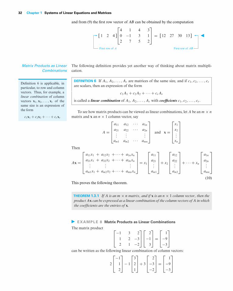
32 Chapter 1 Systems of Linear Equations and Matrices
and from (9) the first row vector of AB can be obtained by the computation
1 2 4
⎡⎢⎣
4 1 4 30 1 3 12 7 5 2
⎤⎥⎦ = 12 27 30 13
First row of A First row of AB
[ ][ ]
Matrix Products as LinearCombinations
The following definition provides yet another way of thinking about matrix multipli-cation.
Definition 6 is applicable, inparticular, to row and columnvectors. Thus, for example, alinear combination of columnvectors x1, x2, . . . , xr of thesame size is an expression ofthe form
c1x1 + c2x2 + · · · + crxr
DEFINITION 6 If A1, A2, . . . , Ar are matrices of the same size, and if c1, c2, . . . , cr
are scalars, then an expression of the form
c1A1 + c2A2 + · · · + crAr
is called a linear combination of A1, A2, . . . , Ar with coefficients c1, c2, . . . , cr .
To see how matrix products can be viewed as linear combinations, let A be an m × n
matrix and x an n × 1 column vector, say
A =
⎡⎢⎢⎢⎣
a11 a12 · · · a1n
a21 a22 · · · a2n...
......
am1 am2 · · · amn
⎤⎥⎥⎥⎦ and x =
⎡⎢⎢⎢⎣
x1
x2...xn
⎤⎥⎥⎥⎦
Then
Ax =
⎡⎢⎢⎢⎣
a11x1 + a12x2 + · · ·+ a1nxn
a21x1 + a22x2 + · · ·+ a2nxn...
......
am1x1 + am2x2 + · · ·+ amnxn
⎤⎥⎥⎥⎦= x1
⎡⎢⎢⎢⎣
a11
a21...
am1
⎤⎥⎥⎥⎦+ x2
⎡⎢⎢⎢⎣
a12
a22...
am2
⎤⎥⎥⎥⎦+ · · · + xn
⎡⎢⎢⎢⎣
a1n
a2n...
amn
⎤⎥⎥⎥⎦
(10)This proves the following theorem.
THEOREM 1.3.1 If A is an m × n matrix, and if x is an n × 1 column vector, then theproductAx can be expressed as a linear combination of the column vectors ofA in whichthe coefficients are the entries of x.
EXAMPLE 8 Matrix Products as Linear Combinations
The matrix product ⎡⎢⎣−1 3 2
1 2 −3
2 1 −2
⎤⎥⎦⎡⎢⎣ 2
−1
3
⎤⎥⎦ =
⎡⎢⎣ 1
−9
−3
⎤⎥⎦
can be written as the following linear combination of column vectors:
2
⎡⎢⎣−1
1
2
⎤⎥⎦− 1
⎡⎢⎣3
2
1
⎤⎥⎦+ 3
⎡⎢⎣ 2
−3
−2
⎤⎥⎦ =
⎡⎢⎣ 1
−9
−3
⎤⎥⎦
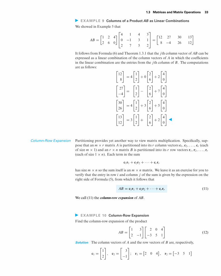
1.3 Matrices and Matrix Operations 33
EXAMPLE 9 Columns of a ProductAB as Linear Combinations
We showed in Example 5 that
AB =[
1 2 4
2 6 0
]⎡⎢⎣4 1 4 3
0 −1 3 1
2 7 5 2
⎤⎥⎦ =
[12 27 30 13
8 −4 26 12
]
It follows from Formula (6) and Theorem 1.3.1 that the j th column vector of AB can beexpressed as a linear combination of the column vectors of A in which the coefficientsin the linear combination are the entries from the j th column of B. The computationsare as follows: [
12
8
]= 4
[1
2
]+ 0
[2
6
]+ 2
[4
0
][
27
−4
]=
[1
2
]−
[2
6
]+ 7
[4
0
][
30
26
]= 4
[1
2
]+ 3
[2
6
]+ 5
[4
0
][
13
12
]= 3
[1
2
]+
[2
6
]+ 2
[4
0
]
Column-Row Expansion Partitioning provides yet another way to view matrix multiplication. Specifically, sup-pose that an m × r matrix A is partitioned into its r column vectors c1, c2, . . . , cr (eachof size m × 1) and an r × n matrix B is partitioned into its r row vectors r1, r2, . . . , rr
(each of size 1 × n). Each term in the sum
c1r1 + c2r2 + · · · + crrr
has size m × n so the sum itself is an m × n matrix. We leave it as an exercise for you toverify that the entry in row i and column j of the sum is given by the expression on theright side of Formula (5), from which it follows that
AB = c1r1 + c2r2 + · · · + crrr (11)
We call (11) the column-row expansion of AB.
EXAMPLE 10 Column-Row Expansion
Find the column-row expansion of the product
AB =[
1 3
2 −1
][2 0 4
−3 5 1
](12)
Solution The column vectors of A and the row vectors of B are, respectively,
c1 =[
1
2
], c2 =
[3
−1
]; r1 = [
2 0 4], r2 = [−3 5 1
]
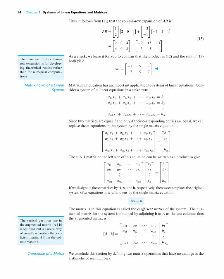
34 Chapter 1 Systems of Linear Equations and Matrices
Thus, it follows from (11) that the column-row expansion of AB is
AB =[
1
2
] [2 0 4
]+[
3
−1
] [−3 5 1]
=[
2 0 4
4 0 8
]+[−9 15 3
3 −5 −1
] (13)
As a check, we leave it for you to confirm that the product in (12) and the sum in (13)The main use of the column-row expansion is for develop-ing theoretical results ratherthan for numerical computa-tions.
both yield
AB =[−7 15 7
7 −5 7
]
Matrix Form of a LinearSystem
Matrix multiplication has an important application to systems of linear equations. Con-sider a system of m linear equations in n unknowns:
a11x1 + a12x2 + · · ·+ a1nxn = b1
a21x1 + a22x2 + · · ·+ a2nxn = b2...
......
...
am1x1 + am2x2 + · · ·+ amnxn = bm
Since two matrices are equal if and only if their corresponding entries are equal, we canreplace the m equations in this system by the single matrix equation⎡
⎢⎢⎢⎣a11x1 + a12x2 + · · ·+ a1nxn
a21x1 + a22x2 + · · ·+ a2nxn...
......
am1x1 + am2x2 + · · ·+ amnxn
⎤⎥⎥⎥⎦ =
⎡⎢⎢⎢⎣
b1
b2...
bm
⎤⎥⎥⎥⎦
The m × 1 matrix on the left side of this equation can be written as a product to give⎡⎢⎢⎢⎣
a11 a12 · · · a1n
a21 a22 · · · a2n...
......
am1 am2 · · · amn
⎤⎥⎥⎥⎦⎡⎢⎢⎢⎣
x1
x2...
xn
⎤⎥⎥⎥⎦ =
⎡⎢⎢⎢⎣
b1
b2...
bm
⎤⎥⎥⎥⎦
If we designate these matrices by A, x, and b, respectively, then we can replace the originalsystem of m equations in n unknowns by the single matrix equation
Ax = b
The matrix A in this equation is called the coefficient matrix of the system. The aug-mented matrix for the system is obtained by adjoining b to A as the last column; thus
The vertical partition line inthe augmented matrix [A | b]is optional, but is a useful wayof visually separating the coef-ficient matrix A from the col-umn vector b.
the augmented matrix is
[A | b] =
⎡⎢⎢⎢⎣
a11 a12 · · · a1n b1
a21 a22 · · · a2n b2...
......
...
am1 am2 · · · amn bm
⎤⎥⎥⎥⎦
Transpose of a Matrix We conclude this section by defining two matrix operations that have no analogs in thearithmetic of real numbers.
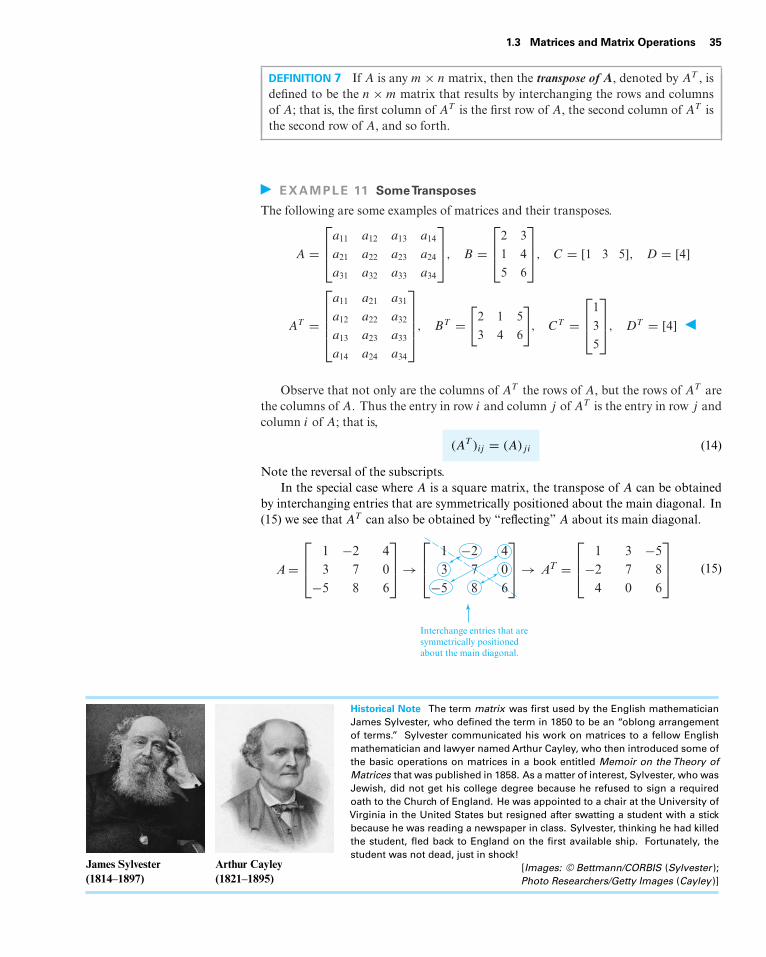
1.3 Matrices and Matrix Operations 35
DEFINITION 7 If A is any m × n matrix, then the transpose of A, denoted by AT , isdefined to be the n × m matrix that results by interchanging the rows and columnsof A; that is, the first column of AT is the first row of A, the second column of AT isthe second row of A, and so forth.
EXAMPLE 11 SomeTransposes
The following are some examples of matrices and their transposes.
A =⎡⎢⎣a11 a12 a13 a14
a21 a22 a23 a24
a31 a32 a33 a34
⎤⎥⎦, B =
⎡⎢⎣2 3
1 4
5 6
⎤⎥⎦, C = [1 3 5], D = [4]
AT =
⎡⎢⎢⎢⎣
a11 a21 a31
a12 a22 a32
a13 a23 a33
a14 a24 a34
⎤⎥⎥⎥⎦, BT =
[2 1 5
3 4 6
], CT =
⎡⎢⎣1
3
5
⎤⎥⎦, DT = [4]
Observe that not only are the columns of AT the rows of A, but the rows of AT arethe columns of A. Thus the entry in row i and column j of AT is the entry in row j andcolumn i of A; that is,
(AT )ij = (A)ji (14)
Note the reversal of the subscripts.In the special case where A is a square matrix, the transpose of A can be obtained
by interchanging entries that are symmetrically positioned about the main diagonal. In(15) we see that AT can also be obtained by “reflecting” A about its main diagonal.
A =
⎡⎢⎣
1 2 43 7 05 8 6
⎤⎥⎦
⎡⎢⎣
1 2 43 7 05 8 6
⎤⎥⎦ AT
⎡⎢⎣
1 3 52 7 84 0 6
⎤⎥⎦
Interchange entries that aresymmetrically positionedabout the main diagonal.
(15)
James Sylvester(1814–1897)
Arthur Cayley(1821–1895)
Historical Note The term matrix was first used by the English mathematicianJames Sylvester, who defined the term in 1850 to be an “oblong arrangementof terms.” Sylvester communicated his work on matrices to a fellow Englishmathematician and lawyer named Arthur Cayley, who then introduced some ofthe basic operations on matrices in a book entitled Memoir on the Theory ofMatrices that was published in 1858. As a matter of interest, Sylvester, who wasJewish, did not get his college degree because he refused to sign a requiredoath to the Church of England. He was appointed to a chair at the University ofVirginia in the United States but resigned after swatting a student with a stickbecause he was reading a newspaper in class. Sylvester, thinking he had killedthe student, fled back to England on the first available ship. Fortunately, thestudent was not dead, just in shock!
[Images: © Bettmann/CORBIS (Sylvester );Photo Researchers/Getty Images (Cayley )]
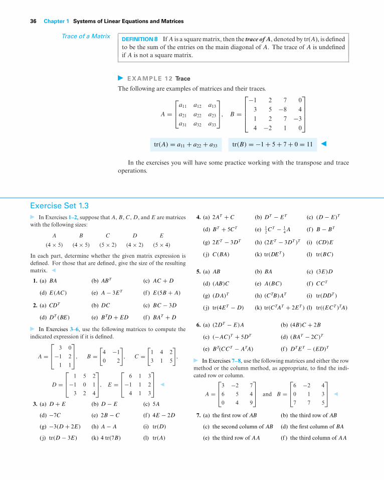
36 Chapter 1 Systems of Linear Equations and Matrices
Trace of a Matrix DEFINITION 8 If A is a square matrix, then the trace of A, denoted by tr(A), is definedto be the sum of the entries on the main diagonal of A. The trace of A is undefinedif A is not a square matrix.
EXAMPLE 12 Trace
The following are examples of matrices and their traces.
A =⎡⎢⎣a11 a12 a13
a21 a22 a23
a31 a32 a33
⎤⎥⎦, B =
⎡⎢⎢⎢⎣−1 2 7 0
3 5 −8 4
1 2 7 −3
4 −2 1 0
⎤⎥⎥⎥⎦
tr(A) = a11 + a22 + a33 tr(B) = −1 + 5 + 7 + 0 = 11
In the exercises you will have some practice working with the transpose and traceoperations.
Exercise Set 1.3
In Exercises 1–2, suppose that A, B, C, D, and E are matriceswith the following sizes:
A B C D E
(4 × 5) (4 × 5) (5 × 2) (4 × 2) (5 × 4)
In each part, determine whether the given matrix expression isdefined. For those that are defined, give the size of the resultingmatrix.
1. (a) BA (b) ABT (c) AC + D
(d) E(AC) (e) A − 3ET (f ) E(5B + A)
2. (a) CDT (b) DC (c) BC − 3D
(d) DT (BE) (e) BTD + ED (f ) BAT + D
In Exercises 3–6, use the following matrices to compute theindicated expression if it is defined.
A =⎡⎢⎣ 3 0
−1 2
1 1
⎤⎥⎦, B =
[4 −1
0 2
], C =
[1 4 2
3 1 5
],
D =⎡⎢⎣ 1 5 2
−1 0 1
3 2 4
⎤⎥⎦, E =
⎡⎢⎣ 6 1 3
−1 1 2
4 1 3
⎤⎥⎦
3. (a) D + E (b) D − E (c) 5A
(d) −7C (e) 2B − C (f ) 4E − 2D
(g) −3(D + 2E) (h) A − A (i) tr(D)
( j) tr(D − 3E) (k) 4 tr(7B) (l) tr(A)
4. (a) 2AT + C (b) DT − ET (c) (D − E)T
(d) BT + 5CT (e) 12 C
T − 14 A (f ) B − BT
(g) 2ET − 3DT (h) (2ET − 3DT )T (i) (CD)E
( j) C(BA) (k) tr(DET ) (l) tr(BC)
5. (a) AB (b) BA (c) (3E)D
(d) (AB)C (e) A(BC) (f ) CCT
(g) (DA)T (h) (CTB)AT (i) tr(DDT )
( j) tr(4ET − D) (k) tr(CTAT + 2ET ) (l) tr((ECT )TA)
6. (a) (2DT − E)A (b) (4B)C + 2B
(c) (−AC)T + 5DT (d) (BAT − 2C)T
(e) BT(CCT − ATA) (f ) DTET − (ED)T
In Exercises 7–8, use the following matrices and either the rowmethod or the column method, as appropriate, to find the indi-cated row or column.
A =⎡⎢⎣3 −2 7
6 5 4
0 4 9
⎤⎥⎦ and B =
⎡⎢⎣6 −2 4
0 1 3
7 7 5
⎤⎥⎦
7. (a) the first row of AB (b) the third row of AB
(c) the second column of AB (d) the first column of BA
(e) the third row of AA (f ) the third column of AA
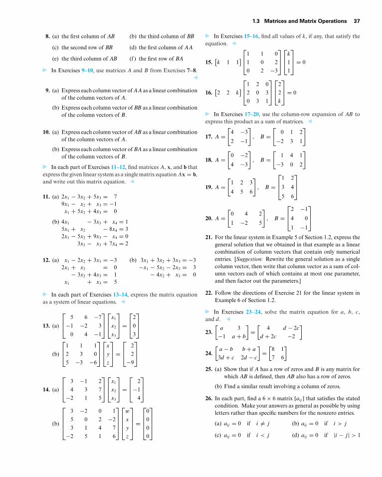
1.3 Matrices and Matrix Operations 37
8. (a) the first column of AB (b) the third column of BB
(c) the second row of BB (d) the first column of AA
(e) the third column of AB (f ) the first row of BA
In Exercises 9–10, use matrices A and B from Exercises 7–8.
9. (a) Express each column vector of AA as a linear combinationof the column vectors of A.
(b) Express each column vector of BB as a linear combinationof the column vectors of B.
10. (a) Express each column vector of AB as a linear combinationof the column vectors of A.
(b) Express each column vector of BA as a linear combinationof the column vectors of B.
In each part of Exercises 11–12, find matrices A, x, and b thatexpress the given linear system as a single matrix equation Ax = b,and write out this matrix equation.
11. (a) 2x1 − 3x2 + 5x3 = 79x1 − x2 + x3 = −1x1 + 5x2 + 4x3 = 0
(b) 4x1 − 3x3 + x4 = 15x1 + x2 − 8x4 = 32x1 − 5x2 + 9x3 − x4 = 0
3x2 − x3 + 7x4 = 2
12. (a) x1 − 2x2 + 3x3 = −32x1 + x2 = 0
− 3x2 + 4x3 = 1x1 + x3 = 5
(b) 3x1 + 3x2 + 3x3 = −3−x1 − 5x2 − 2x3 = 3
− 4x2 + x3 = 0
In each part of Exercises 13–14, express the matrix equationas a system of linear equations.
13. (a)
⎡⎢⎣ 5 6 −7
−1 −2 3
0 4 −1
⎤⎥⎦⎡⎢⎣x1
x2
x3
⎤⎥⎦ =
⎡⎢⎣2
0
3
⎤⎥⎦
(b)
⎡⎢⎣1 1 1
2 3 0
5 −3 −6
⎤⎥⎦⎡⎢⎣x
y
z
⎤⎥⎦ =
⎡⎢⎣ 2
2
−9
⎤⎥⎦
14. (a)
⎡⎢⎣ 3 −1 2
4 3 7
−2 1 5
⎤⎥⎦⎡⎢⎣x1
x2
x3
⎤⎥⎦ =
⎡⎢⎣ 2
−1
4
⎤⎥⎦
(b)
⎡⎢⎢⎢⎣
3 −2 0 1
5 0 2 −2
3 1 4 7
−2 5 1 6
⎤⎥⎥⎥⎦⎡⎢⎢⎢⎣
w
x
y
z
⎤⎥⎥⎥⎦ =
⎡⎢⎢⎢⎣
0
0
0
0
⎤⎥⎥⎥⎦
In Exercises 15–16, find all values of k, if any, that satisfy theequation.
15.[k 1 1
]⎡⎢⎣1 1 0
1 0 2
0 2 −3
⎤⎥⎦⎡⎢⎣k
1
1
⎤⎥⎦ = 0
16.[2 2 k
]⎡⎢⎣1 2 0
2 0 3
0 3 1
⎤⎥⎦⎡⎢⎣2
2
k
⎤⎥⎦ = 0
In Exercises 17–20, use the column-row expansion of AB toexpress this product as a sum of matrices.
17. A =[
4 −3
2 −1
], B =
[0 1 2
−2 3 1
]
18. A =[
0 −2
4 −3
], B =
[1 4 1
−3 0 2
]
19. A =[
1 2 3
4 5 6
], B =
⎡⎢⎣
1 2
3 4
5 6
⎤⎥⎦
20. A =[
0 4 2
1 −2 5
], B =
⎡⎢⎣
2 −1
4 0
1 −1
⎤⎥⎦
21. For the linear system in Example 5 of Section 1.2, express thegeneral solution that we obtained in that example as a linearcombination of column vectors that contain only numericalentries. [Suggestion: Rewrite the general solution as a singlecolumn vector, then write that column vector as a sum of col-umn vectors each of which contains at most one parameter,and then factor out the parameters.]
22. Follow the directions of Exercise 21 for the linear system inExample 6 of Section 1.2.
In Exercises 23–24, solve the matrix equation for a, b, c,and d.
23.[
a 3
−1 a + b
]=[
4 d − 2c
d + 2c −2
]
24.[
a − b b + a
3d + c 2d − c
]=[
8 1
7 6
]
25. (a) Show that if A has a row of zeros and B is any matrix forwhich AB is defined, then AB also has a row of zeros.
(b) Find a similar result involving a column of zeros.
26. In each part, find a 6 × 6 matrix [aij ] that satisfies the statedcondition. Make your answers as general as possible by usingletters rather than specific numbers for the nonzero entries.
(a) aij = 0 if i �= j (b) aij = 0 if i > j
(c) aij = 0 if i < j (d) aij = 0 if |i − j | > 1
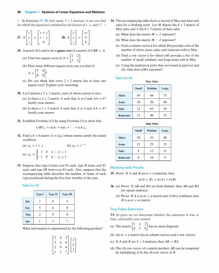
38 Chapter 1 Systems of Linear Equations and Matrices
In Exercises 27–28, how many 3 × 3 matrices A can you findfor which the equation is satisfied for all choices of x, y, and z?
27. A
⎡⎢⎣x
y
z
⎤⎥⎦ =
⎡⎢⎣x + y
x − y
0
⎤⎥⎦ 28. A
⎡⎢⎣x
y
z
⎤⎥⎦ =
⎡⎢⎣xy
0
0
⎤⎥⎦
29. A matrix B is said to be a square root of a matrix A if BB = A.
(a) Find two square roots of A =[
2 2
2 2
].
(b) How many different square roots can you find of
A =[
5 0
0 9
]?
(c) Do you think that every 2 × 2 matrix has at least onesquare root? Explain your reasoning.
30. Let 0 denote a 2 × 2 matrix, each of whose entries is zero.
(a) Is there a 2 × 2 matrix A such that A �= 0 and AA = 0 ?Justify your answer.
(b) Is there a 2 × 2 matrix A such that A �= 0 and AA = A?Justify your answer.
31. Establish Formula (11) by using Formula (5) to show that
(AB)ij = (c1r1 + c2r2 + · · · + crrr )ij
32. Find a 4 × 4 matrix A = [aij ] whose entries satisfy the statedcondition.
(a) aij = i + j (b) aij = ij−1
(c) aij ={
1 if |i − j | > 1
−1 if |i − j | ≤ 1
33. Suppose that type I items cost $1 each, type II items cost $2each, and type III items cost $3 each. Also, suppose that theaccompanying table describes the number of items of eachtype purchased during the first four months of the year.
Table Ex-33
Type I Type II Type III
Jan. 3 4 3
Feb. 5 6 0
Mar. 2 9 4
Apr. 1 1 7
What information is represented by the following product?
⎡⎢⎢⎢⎣
3 4 3
5 6 0
2 9 4
1 1 7
⎤⎥⎥⎥⎦⎡⎢⎣1
2
3
⎤⎥⎦
34. The accompanying table shows a record of May and June unitsales for a clothing store. Let M denote the 4 × 3 matrix ofMay sales and J the 4 × 3 matrix of June sales.
(a) What does the matrix M + J represent?
(b) What does the matrix M − J represent?
(c) Find a column vector x for which Mx provides a list of thenumber of shirts, jeans, suits, and raincoats sold in May.
(d) Find a row vector y for which yM provides a list of thenumber of small, medium, and large items sold in May.
(e) Using the matrices x and y that you found in parts (c) and(d), what does yMx represent?
Table Ex-34May Sales
Small Medium Large
Shirts 45 60 75
Jeans 30 30 40
Suits 12 65 45
Raincoats 15 40 35
June Sales
Small Medium Large
Shirts 30 33 40
Jeans 21 23 25
Suits 9 12 11
Raincoats 8 10 9
Working with Proofs
35. Prove: If A and B are n × n matrices, then
tr(A + B) = tr(A) + tr(B)
36. (a) Prove: If AB and BA are both defined, then AB and BA
are square matrices.
(b) Prove: If A is an m × n matrix and A(BA) is defined, thenB is an n × m matrix.
True-False Exercises
TF. In parts (a)–(o) determine whether the statement is true orfalse, and justify your answer.
(a) The matrix
[1 2 34 5 6
]has no main diagonal.
(b) An m × n matrix has m column vectors and n row vectors.
(c) If A and B are 2 × 2 matrices, then AB = BA.
(d) The ith row vector of a matrix product AB can be computedby multiplying A by the ith row vector of B.
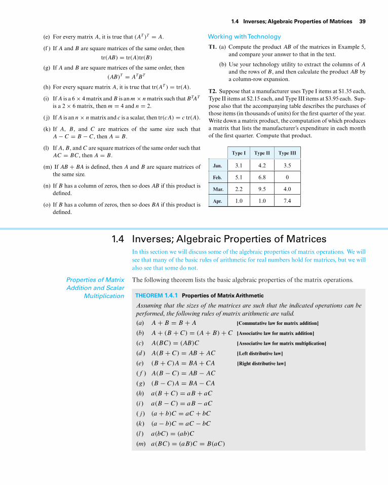
1.4 Inverses; Algebraic Properties of Matrices 39
(e) For every matrix A, it is true that (AT )T = A.
(f ) If A and B are square matrices of the same order, then
tr(AB) = tr(A)tr(B)
(g) If A and B are square matrices of the same order, then
(AB)T = ATBT
(h) For every square matrix A, it is true that tr(AT ) = tr(A).
(i) If A is a 6 × 4 matrix and B is an m × n matrix such that BTAT
is a 2 × 6 matrix, then m = 4 and n = 2.
( j) If A is an n × n matrix and c is a scalar, then tr(cA) = c tr(A).
(k) If A, B, and C are matrices of the same size such thatA − C = B − C, then A = B.
(l) If A, B, and C are square matrices of the same order such thatAC = BC, then A = B.
(m) If AB + BA is defined, then A and B are square matrices ofthe same size.
(n) If B has a column of zeros, then so does AB if this product isdefined.
(o) If B has a column of zeros, then so does BA if this product isdefined.
Working withTechnology
T1. (a) Compute the product AB of the matrices in Example 5,and compare your answer to that in the text.
(b) Use your technology utility to extract the columns of A
and the rows of B, and then calculate the product AB bya column-row expansion.
T2. Suppose that a manufacturer uses Type I items at $1.35 each,Type II items at $2.15 each, and Type III items at $3.95 each. Sup-pose also that the accompanying table describes the purchases ofthose items (in thousands of units) for the first quarter of the year.Write down a matrix product, the computation of which producesa matrix that lists the manufacturer’s expenditure in each monthof the first quarter. Compute that product.
Type I Type II Type III
Jan. 3.1 4.2 3.5
Feb. 5.1 6.8 0
Mar. 2.2 9.5 4.0
Apr. 1.0 1.0 7.4
1.4 Inverses; Algebraic Properties of MatricesIn this section we will discuss some of the algebraic properties of matrix operations. We willsee that many of the basic rules of arithmetic for real numbers hold for matrices, but we willalso see that some do not.
Properties of MatrixAddition and Scalar
Multiplication
The following theorem lists the basic algebraic properties of the matrix operations.
THEOREM 1.4.1 Properties of Matrix Arithmetic
Assuming that the sizes of the matrices are such that the indicated operations can beperformed, the following rules of matrix arithmetic are valid.
(a) A + B = B + A [Commutative law for matrix addition]
(b) A + (B + C) = (A + B) + C [Associative law for matrix addition]
(c) A(BC) = (AB)C [Associative law for matrix multiplication]
(d ) A(B + C) = AB + AC [Left distributive law]
(e) (B + C)A = BA + CA [Right distributive law]
( f ) A(B − C) = AB − AC
(g) (B − C)A = BA − CA
(h) a(B + C) = aB + aC
(i ) a(B − C) = aB − aC
( j ) (a + b)C = aC + bC
(k) (a − b)C = aC − bC
(l ) a(bC) = (ab)C
(m) a(BC) = (aB)C = B(aC)
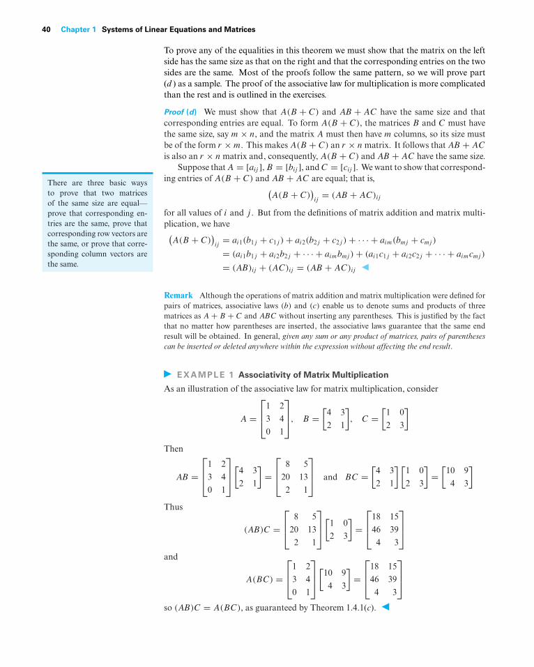
40 Chapter 1 Systems of Linear Equations and Matrices
To prove any of the equalities in this theorem we must show that the matrix on the leftside has the same size as that on the right and that the corresponding entries on the twosides are the same. Most of the proofs follow the same pattern, so we will prove part(d ) as a sample. The proof of the associative law for multiplication is more complicatedthan the rest and is outlined in the exercises.
Proof (d) We must show that A(B + C) and AB + AC have the same size and thatcorresponding entries are equal. To form A(B + C), the matrices B and C must havethe same size, say m × n, and the matrix A must then have m columns, so its size mustbe of the form r × m. This makes A(B + C) an r × n matrix. It follows that AB + AC
is also an r × n matrix and, consequently, A(B + C) and AB + AC have the same size.Suppose that A = [aij ], B = [bij ], and C = [cij ]. We want to show that correspond-
ing entries of A(B + C) and AB + AC are equal; that is,(A(B + C)
)ij= (AB + AC)ij
for all values of i and j . But from the definitions of matrix addition and matrix multi-
There are three basic waysto prove that two matricesof the same size are equal—prove that corresponding en-tries are the same, prove thatcorresponding row vectors arethe same, or prove that corre-sponding column vectors arethe same.
plication, we have(A(B + C)
)ij= ai1(b1j + c1j ) + ai2(b2j + c2j ) + · · · + aim(bmj + cmj )
= (ai1b1j + ai2b2j + · · · + aimbmj ) + (ai1c1j + ai2c2j + · · · + aimcmj )
= (AB)ij + (AC)ij = (AB + AC)ij
Remark Although the operations of matrix addition and matrix multiplication were defined forpairs of matrices, associative laws (b) and (c) enable us to denote sums and products of threematrices as A + B + C and ABC without inserting any parentheses. This is justified by the factthat no matter how parentheses are inserted, the associative laws guarantee that the same endresult will be obtained. In general, given any sum or any product of matrices, pairs of parenthesescan be inserted or deleted anywhere within the expression without affecting the end result.
EXAMPLE 1 Associativity of Matrix Multiplication
As an illustration of the associative law for matrix multiplication, consider
A =⎡⎢⎣1 2
3 4
0 1
⎤⎥⎦, B =
[4 3
2 1
], C =
[1 0
2 3
]
Then
AB =⎡⎢⎣1 2
3 4
0 1
⎤⎥⎦[4 3
2 1
]=⎡⎢⎣ 8 5
20 13
2 1
⎤⎥⎦ and BC =
[4 3
2 1
] [1 0
2 3
]=[
10 9
4 3
]
Thus
(AB)C =⎡⎢⎣ 8 5
20 13
2 1
⎤⎥⎦[1 0
2 3
]=⎡⎢⎣18 15
46 39
4 3
⎤⎥⎦
and
A(BC) =⎡⎢⎣1 2
3 4
0 1
⎤⎥⎦[10 9
4 3
]=⎡⎢⎣18 15
46 39
4 3
⎤⎥⎦
so (AB)C = A(BC), as guaranteed by Theorem 1.4.1(c).
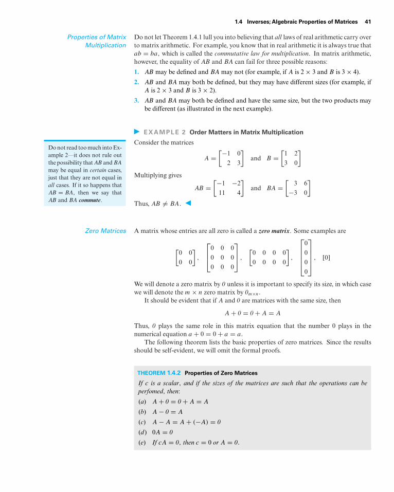
1.4 Inverses; Algebraic Properties of Matrices 41
Properties of MatrixMultiplication
Do not let Theorem 1.4.1 lull you into believing that all laws of real arithmetic carry overto matrix arithmetic. For example, you know that in real arithmetic it is always true thatab = ba, which is called the commutative law for multiplication. In matrix arithmetic,however, the equality of AB and BA can fail for three possible reasons:
1. AB may be defined and BA may not (for example, if A is 2 × 3 and B is 3 × 4).
2. AB and BA may both be defined, but they may have different sizes (for example, ifA is 2 × 3 and B is 3 × 2).
3. AB and BA may both be defined and have the same size, but the two products maybe different (as illustrated in the next example).
EXAMPLE 2 Order Matters in Matrix Multiplication
Consider the matricesDo not read too much into Ex-ample 2—it does not rule outthe possibility that AB and BA
may be equal in certain cases,just that they are not equal inall cases. If it so happens thatAB = BA, then we say thatAB and BA commute.
A =[−1 0
2 3
]and B =
[1 2
3 0
]Multiplying gives
AB =[−1 −2
11 4
]and BA =
[3 6
−3 0
]Thus, AB �= BA.
Zero Matrices A matrix whose entries are all zero is called a zero matrix. Some examples are
[0 0
0 0
],
⎡⎢⎣0 0 0
0 0 0
0 0 0
⎤⎥⎦ ,
[0 0 0 0
0 0 0 0
],
⎡⎢⎢⎢⎣
0
0
0
0
⎤⎥⎥⎥⎦ , [0]
We will denote a zero matrix by 0 unless it is important to specify its size, in which casewe will denote the m × n zero matrix by 0m×n.
It should be evident that if A and 0 are matrices with the same size, then
A + 0 = 0+ A = A
Thus, 0 plays the same role in this matrix equation that the number 0 plays in thenumerical equation a + 0 = 0 + a = a.
The following theorem lists the basic properties of zero matrices. Since the resultsshould be self-evident, we will omit the formal proofs.
THEOREM 1.4.2 Properties of Zero Matrices
If c is a scalar, and if the sizes of the matrices are such that the operations can beperfomed, then:
(a) A + 0 = 0+ A = A
(b) A − 0 = A
(c) A − A = A + (−A) = 0
(d ) 0A = 0
(e) If cA = 0, then c = 0 or A = 0.
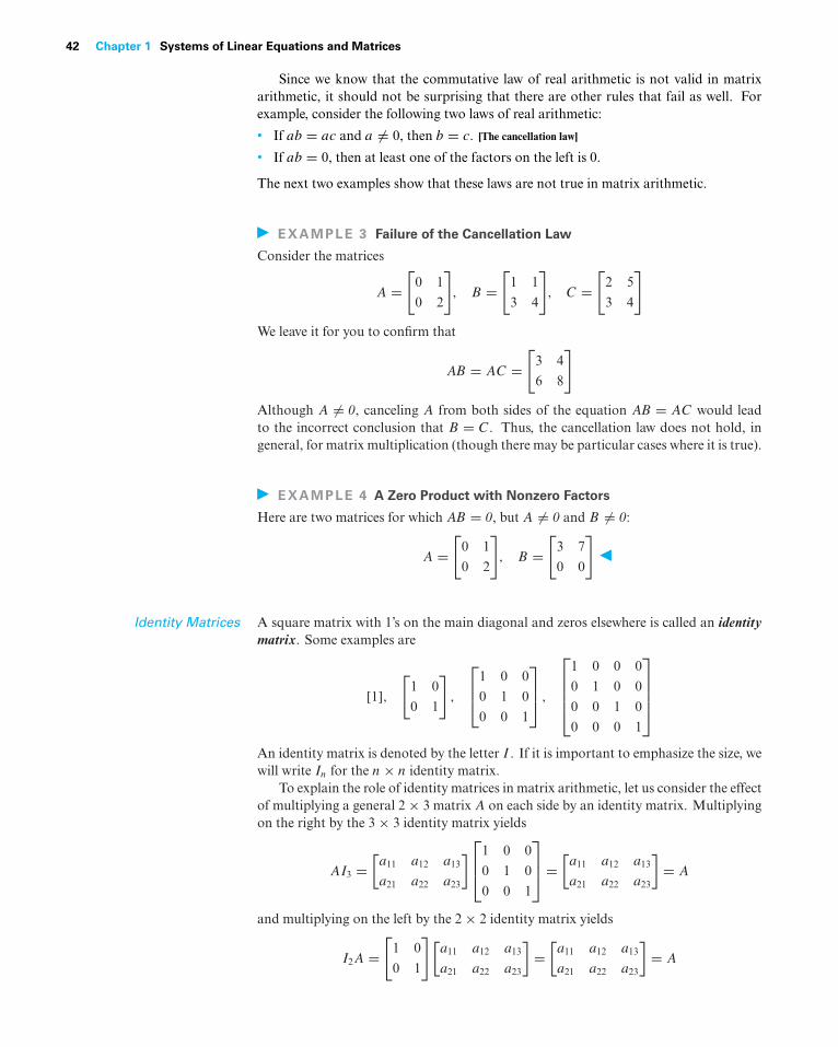
42 Chapter 1 Systems of Linear Equations and Matrices
Since we know that the commutative law of real arithmetic is not valid in matrixarithmetic, it should not be surprising that there are other rules that fail as well. Forexample, consider the following two laws of real arithmetic:
• If ab = ac and a �= 0, then b = c. [The cancellation law]
• If ab = 0, then at least one of the factors on the left is 0.
The next two examples show that these laws are not true in matrix arithmetic.
EXAMPLE 3 Failure of the Cancellation Law
Consider the matrices
A =[
0 1
0 2
], B =
[1 1
3 4
], C =
[2 5
3 4
]
We leave it for you to confirm that
AB = AC =[
3 4
6 8
]
Although A �= 0, canceling A from both sides of the equation AB = AC would leadto the incorrect conclusion that B = C. Thus, the cancellation law does not hold, ingeneral, for matrix multiplication (though there may be particular cases where it is true).
EXAMPLE 4 A Zero Product with Nonzero Factors
Here are two matrices for which AB = 0, but A �= 0 and B �= 0:
A =[
0 1
0 2
], B =
[3 7
0 0
]
Identity Matrices A square matrix with 1’s on the main diagonal and zeros elsewhere is called an identitymatrix. Some examples are
[1],[
1 0
0 1
],
⎡⎢⎣1 0 0
0 1 0
0 0 1
⎤⎥⎦ ,
⎡⎢⎢⎢⎣
1 0 0 0
0 1 0 0
0 0 1 0
0 0 0 1
⎤⎥⎥⎥⎦
An identity matrix is denoted by the letter I . If it is important to emphasize the size, wewill write In for the n × n identity matrix.
To explain the role of identity matrices in matrix arithmetic, let us consider the effectof multiplying a general 2 × 3 matrix A on each side by an identity matrix. Multiplyingon the right by the 3 × 3 identity matrix yields
AI3 =[a11 a12 a13
a21 a22 a23
]⎡⎢⎣1 0 0
0 1 0
0 0 1
⎤⎥⎦ =
[a11 a12 a13
a21 a22 a23
]= A
and multiplying on the left by the 2 × 2 identity matrix yields
I2A =[
1 0
0 1
][a11 a12 a13
a21 a22 a23
]=[a11 a12 a13
a21 a22 a23
]= A
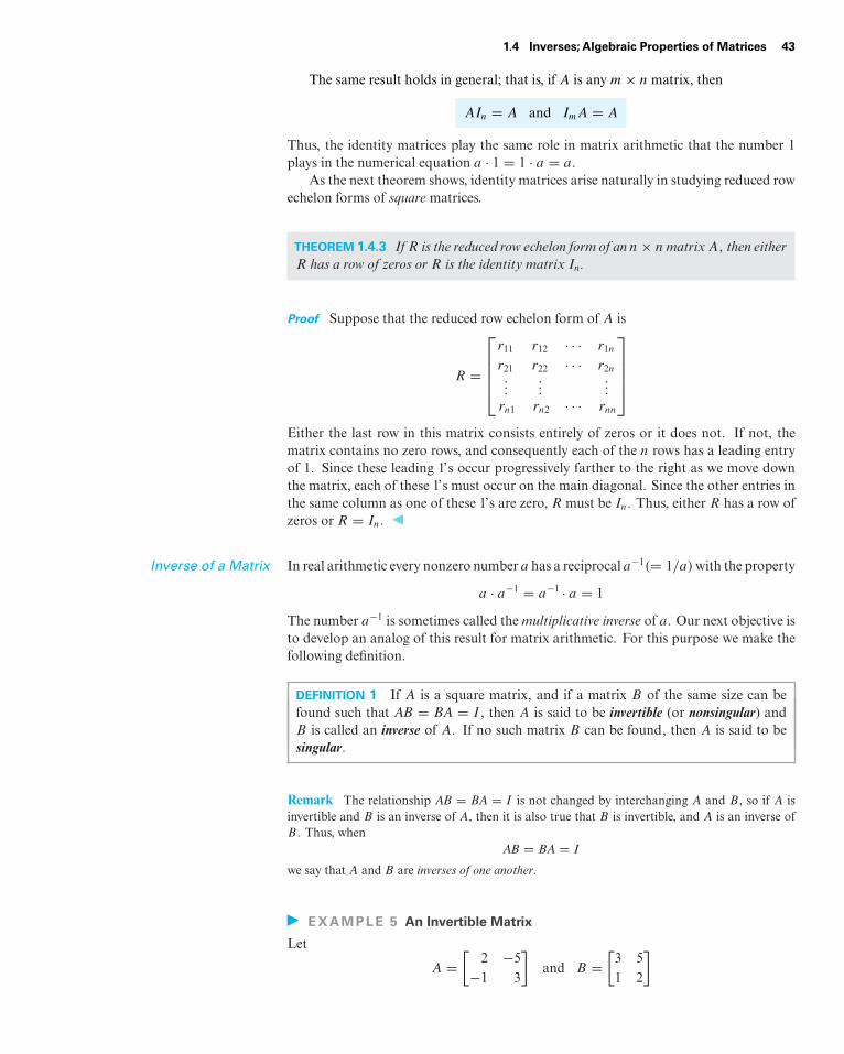
1.4 Inverses; Algebraic Properties of Matrices 43
The same result holds in general; that is, if A is any m × n matrix, then
AIn = A and ImA = A
Thus, the identity matrices play the same role in matrix arithmetic that the number 1plays in the numerical equation a · 1 = 1 · a = a.
As the next theorem shows, identity matrices arise naturally in studying reduced rowechelon forms of square matrices.
THEOREM 1.4.3 IfR is the reduced row echelon form of an n × nmatrixA, then eitherR has a row of zeros or R is the identity matrix In.
Proof Suppose that the reduced row echelon form of A is
R =
⎡⎢⎢⎢⎣
r11 r12 · · · r1n
r21 r22 · · · r2n...
......
rn1 rn2 · · · rnn
⎤⎥⎥⎥⎦
Either the last row in this matrix consists entirely of zeros or it does not. If not, thematrix contains no zero rows, and consequently each of the n rows has a leading entryof 1. Since these leading 1’s occur progressively farther to the right as we move downthe matrix, each of these 1’s must occur on the main diagonal. Since the other entries inthe same column as one of these 1’s are zero, R must be In. Thus, either R has a row ofzeros or R = In.
Inverse of a Matrix In real arithmetic every nonzero number a has a reciprocal a−1(= 1/a) with the property
a · a−1 = a−1 · a = 1
The number a−1 is sometimes called the multiplicative inverse of a. Our next objective isto develop an analog of this result for matrix arithmetic. For this purpose we make thefollowing definition.
DEFINITION 1 If A is a square matrix, and if a matrix B of the same size can befound such that AB = BA = I , then A is said to be invertible (or nonsingular) andB is called an inverse of A. If no such matrix B can be found, then A is said to besingular.
Remark The relationship AB = BA = I is not changed by interchanging A and B, so if A isinvertible and B is an inverse of A, then it is also true that B is invertible, and A is an inverse ofB. Thus, when
AB = BA = I
we say that A and B are inverses of one another.
EXAMPLE 5 An Invertible Matrix
Let
A =[
2 −5−1 3
]and B =
[3 51 2
]
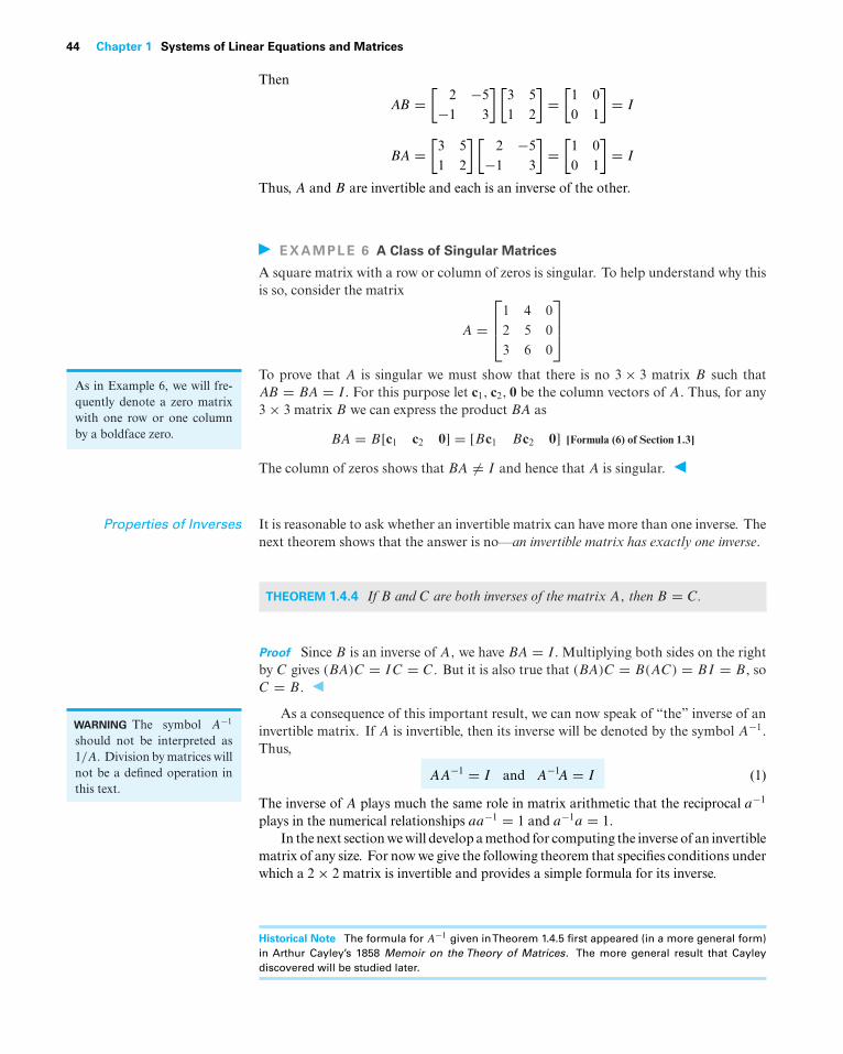
44 Chapter 1 Systems of Linear Equations and Matrices
Then
AB =[
2 −5−1 3
] [3 51 2
]=[
1 00 1
]= I
BA =[
3 51 2
] [2 −5
−1 3
]=[
1 00 1
]= I
Thus, A and B are invertible and each is an inverse of the other.
EXAMPLE 6 A Class of Singular Matrices
A square matrix with a row or column of zeros is singular. To help understand why thisis so, consider the matrix
A =⎡⎢⎣1 4 0
2 5 03 6 0
⎤⎥⎦
To prove that A is singular we must show that there is no 3 × 3 matrix B such thatAs in Example 6, we will fre-quently denote a zero matrixwith one row or one columnby a boldface zero.
AB = BA = I. For this purpose let c1, c2, 0 be the column vectors of A. Thus, for any3 × 3 matrix B we can express the product BA as
BA = B[c1 c2 0] = [Bc1 Bc2 0] [Formula (6) of Section 1.3]
The column of zeros shows that BA �= I and hence that A is singular.
Properties of Inverses It is reasonable to ask whether an invertible matrix can have more than one inverse. Thenext theorem shows that the answer is no—an invertible matrix has exactly one inverse.
THEOREM 1.4.4 If B and C are both inverses of the matrix A, then B = C.
Proof Since B is an inverse of A, we have BA = I. Multiplying both sides on the rightby C gives (BA)C = IC = C. But it is also true that (BA)C = B(AC) = BI = B, soC = B.
As a consequence of this important result, we can now speak of “the” inverse of anWARNING The symbol A−1
should not be interpreted as1/A. Division by matrices willnot be a defined operation inthis text.
invertible matrix. If A is invertible, then its inverse will be denoted by the symbol A−1.
Thus,
AA−1 = I and A−1A = I (1)
The inverse of A plays much the same role in matrix arithmetic that the reciprocal a−1
plays in the numerical relationships aa−1 = 1 and a−1a = 1.In the next section we will develop a method for computing the inverse of an invertible
matrix of any size. For now we give the following theorem that specifies conditions underwhich a 2 × 2 matrix is invertible and provides a simple formula for its inverse.
Historical Note The formula for A−1 given inTheorem 1.4.5 first appeared (in a more general form)
in Arthur Cayley’s 1858 Memoir on the Theory of Matrices. The more general result that Cayley
discovered will be studied later.
1.4 Inverses; Algebraic Properties of Matrices 45
THEOREM 1.4.5 The matrix
A =[a b
c d
]is invertible if and only if ad − bc �= 0, in which case the inverse is given by the formula
A−1 = 1
ad − bc
[d −b
−c a
](2)
We will omit the proof, because we will study a more general version of this theorem
The quantity ad − bc in The-orem 1.4.5 is called the deter-minant of the 2 × 2 matrix A
and is denoted by
det(A) = ad − bc
or alternatively by∣∣∣∣a b
c d
∣∣∣∣ = ad − bc
later. For now, you should at least confirm the validity of Formula (2) by showing thatAA−1 = A−1A = I .
Remark Figure 1.4.1 illustrates that the determinant of a 2 × 2 matrix A is the product of thedet(A) = = ad – bca b
c d
Figure 1.4.1
entries on its main diagonal minus the product of the entries off its main diagonal.
EXAMPLE 7 Calculating the Inverse of a 2 × 2 Matrix
In each part, determine whether the matrix is invertible. If so, find its inverse.
(a) A =[
6 15 2
](b) A =
[−1 23 −6
]Solution (a) The determinant of A is det(A) = (6)(2) − (1)(5) = 7, which is nonzero.Thus, A is invertible, and its inverse is
A−1 = 1
7
[2 −1
−5 6
]=[
27 − 1
7
− 57
67
]
We leave it for you to confirm that AA−1 = A−1A = I.
Solution (b) The matrix is not invertible since det(A) = (−1)(−6) − (2)(3) = 0.
EXAMPLE 8 Solution of a Linear System by Matrix Inversion
A problem that arises in many applications is to solve a pair of equations of the form
u = ax + by
v = cx + dy
for x and y in terms of u and v. One approach is to treat this as a linear system oftwo equations in the unknowns x and y and use Gauss–Jordan elimination to solvefor x and y. However, because the coefficients of the unknowns are literal rather thannumerical, this procedure is a little clumsy. As an alternative approach, let us replace thetwo equations by the single matrix equation[
u
v
]=[ax + by
cx + dy
]which we can rewrite as [
u
v
]=[a b
c d
] [x
y
]If we assume that the 2 × 2 matrix is invertible (i.e., ad − bc �= 0), then we can multiplythrough on the left by the inverse and rewrite the equation as[
a b
c d
]−1 [u
v
]=[a b
c d
]−1 [a b
c d
] [x
y
]
46 Chapter 1 Systems of Linear Equations and Matrices
which simplifies to [a b
c d
]−1 [u
v
]=[x
y
]Using Theorem 1.4.5, we can rewrite this equation as
1
ad − bc
[d −b
−c a
] [u
v
]=[x
y
]from which we obtain
x = du − bv
ad − bc, y = av − cu
ad − bc
The next theorem is concerned with inverses of matrix products.
THEOREM 1.4.6 If A and B are invertible matrices with the same size, then AB isinvertible and
(AB)−1 = B−1A−1
Proof We can establish the invertibility and obtain the stated formula at the same timeby showing that
(AB)(B−1A−1) = (B−1A−1)(AB) = I
But(AB)(B−1A−1) = A(BB−1)A−1 = AIA−1 = AA−1 = I
and similarly, (B−1A−1)(AB) = I.
Although we will not prove it, this result can be extended to three or more factors:
Aproduct of any number of invertiblematrices is invertible, and the inverse of the productis the product of the inverses in the reverse order.
EXAMPLE 9 The Inverse of a Product
Consider the matrices
A =[
1 21 3
], B =
[3 22 2
]We leave it for you to show that
AB =[
7 69 8
], (AB)−1 =
[4 −3
− 92
72
]
and also that
A−1 =[
3 −2−1 1
], B−1 =
[1 −1
−1 32
], B−1A−1 =
[1 −1
−1 32
][3 −2
−1 1
]=[
4 −3
− 92
72
]
Thus, (AB)−1 = B−1A−1 as guaranteed by Theorem 1.4.6.
If a product of matrices issingular, then at least one ofthe factors must be singular.Why?
Powers of a Matrix If A is a square matrix, then we define the nonnegative integer powers of A to be
A0 = I and An = AA · · ·A [n factors]
and if A is invertible, then we define the negative integer powers of A to be
A−n = (A−1)n = A−1A−1 · · ·A−1 [n factors]

1.4 Inverses; Algebraic Properties of Matrices 47
Because these definitions parallel those for real numbers, the usual laws of nonnegativeexponents hold; for example,
ArAs = Ar+s and (Ar)s = Ars
In addition, we have the following properties of negative exponents.
THEOREM 1.4.7 If A is invertible and n is a nonnegative integer, then:
(a) A−1 is invertible and (A−1)−1 = A.
(b) An is invertible and (An)−1 = A−n = (A−1)n.
(c) kA is invertible for any nonzero scalar k, and (kA)−1 = k−1A−1.
We will prove part (c) and leave the proofs of parts (a) and (b) as exercises.
Proof (c) Properties (m) and (l) of Theorem 1.4.1 imply that
(kA)(k−1A−1) = k−1(kA)A−1 = (k−1k)AA−1 = (1)I = I
and similarly, (k−1A−1)(kA) = I. Thus, kA is invertible and (kA)−1 = k−1A−1.
EXAMPLE 10 Properties of Exponents
Let A and A−1 be the matrices in Example 9; that is,
A =[
1 2
1 3
]and A−1 =
[3 −2
−1 1
]Then
A−3 = (A−1)3 =[
3 −2
−1 1
] [3 −2
−1 1
] [3 −2
−1 1
]=[
41 −30
−15 11
]Also,
A3 =[
1 2
1 3
] [1 2
1 3
] [1 2
1 3
]=[
11 30
15 41
]so, as expected from Theorem 1.4.7(b),
(A3)−1 = 1
(11)(41) − (30)(15)
[41 −30
−15 11
]=[
41 −30
−15 11
]= (A−1)3
EXAMPLE 11 The Square of a Matrix Sum
In real arithmetic, where we have a commutative law for multiplication, we can write
(a + b)2 = a2 + ab + ba + b2 = a2 + ab + ab + b2 = a2 + 2ab + b2
However, in matrix arithmetic, where we have no commutative law for multiplication,the best we can do is to write
(A + B)2 = A2 + AB + BA + B2
It is only in the special case where A and B commute (i.e., AB = BA) that we can go astep further and write
(A + B)2 = A2 + 2AB + B2
Matrix Polynomials If A is a square matrix, say n × n, and if
p(x) = a0 + a1x + a2x2 + · · · + amxm
48 Chapter 1 Systems of Linear Equations and Matrices
is any polynomial, then we define the n × n matrix p(A) to be
p(A) = a0I + a1A + a2A2 + · · · + amAm (3)
where I is the n × n identity matrix; that is, p(A) is obtained by substituting A for x
and replacing the constant term a0 by the matrix a0I. An expression of form (3) is calleda matrix polynomial in A.
EXAMPLE 12 A Matrix Polynomial
Find p(A) for
p(x) = x2 − 2x − 3 and A =[−1 2
0 3
]
Solutionp(A) = A2 − 2A − 3I
=[−1 2
0 3
]2
− 2
[−1 2
0 3
]− 3
[1 0
0 1
]
=[
1 4
0 9
]−[−2 4
0 6
]−[
3 0
0 3
]=[
0 0
0 0
]or more briefly, p(A) = 0.
Remark It follows from the fact that ArAs = Ar+s = As+r = AsAr that powers of a squarematrix commute, and since a matrix polynomial in A is built up from powers of A, any two matrixpolynomials in A also commute; that is, for any polynomials p1 and p2 we have
p1(A)p2(A) = p2(A)p1(A) (4)
Properties of theTranspose The following theorem lists the main properties of the transpose.
THEOREM 1.4.8 If the sizes of the matrices are such that the stated operations can beperformed, then:
(a) (AT )T = A
(b) (A + B)T = AT + BT
(c) (A − B)T = AT − BT
(d ) (kA)T = kAT
(e) (AB)T = BTAT
If you keep in mind that transposing a matrix interchanges its rows and columns, thenyou should have little trouble visualizing the results in parts (a)–(d ). For example, part(a) states the obvious fact that interchanging rows and columns twice leaves a matrixunchanged; and part (b) states that adding two matrices and then interchanging therows and columns produces the same result as interchanging the rows and columnsbefore adding. We will omit the formal proofs. Part (e) is less obvious, but for brevitywe will omit its proof as well. The result in that part can be extended to three or morefactors and restated as:
The transpose of a product of any number of matrices is the product of the transposesin the reverse order.
1.4 Inverses; Algebraic Properties of Matrices 49
The following theorem establishes a relationship between the inverse of a matrix andthe inverse of its transpose.
THEOREM 1.4.9 If A is an invertible matrix, then AT is also invertible and
(AT )−1 = (A−1)T
Proof We can establish the invertibility and obtain the formula at the same time byshowing that
AT(A−1)T = (A−1)TAT = I
But from part (e) of Theorem 1.4.8 and the fact that I T = I, we have
AT(A−1)T = (A−1A)T = I T = I
(A−1)TAT = (AA−1)T = I T = I
which completes the proof.
EXAMPLE 13 Inverse of aTranspose
Consider a general 2 × 2 invertible matrix and its transpose:
A =[a b
c d
]and AT =
[a c
b d
]Since A is invertible, its determinant ad − bc is nonzero. But the determinant of AT isalso ad − bc (verify), so AT is also invertible. It follows from Theorem 1.4.5 that
(AT )−1 =
⎡⎢⎢⎣
d
ad − bc− c
ad − bc
− b
ad − bc
a
ad − bc
⎤⎥⎥⎦
which is the same matrix that results if A−1 is transposed (verify). Thus,
(AT )−1 = (A−1)T
as guaranteed by Theorem 1.4.9.
Exercise Set 1.4In Exercises 1–2, verify that the following matrices and scalars
satisfy the stated properties of Theorem 1.4.1.
A =[
3 −1
2 4
], B =
[0 2
1 −4
],
C =[
4 1
−3 −2
], a = 4, b = −7
1. (a) The associative law for matrix addition.
(b) The associative law for matrix multiplication.
(c) The left distributive law.
(d) (a + b)C = aC + bC
2. (a) a(BC) = (aB)C = B(aC)
(b) A(B − C) = AB − AC (c) (B + C)A = BA + CA
(d) a(bC) = (ab)C
In Exercises 3–4, verify that the matrices and scalars in Exer-cise 1 satisfy the stated properties.
3. (a) (AT )T = A (b) (AB)T = BTAT
4. (a) (A + B)T = AT + BT (b) (aC)T = aCT
In Exercises 5–8, use Theorem 1.4.5 to compute the inverse ofthe matrix.
5. A =[
2 −3
4 4
]6. B =
[3 1
5 2
]
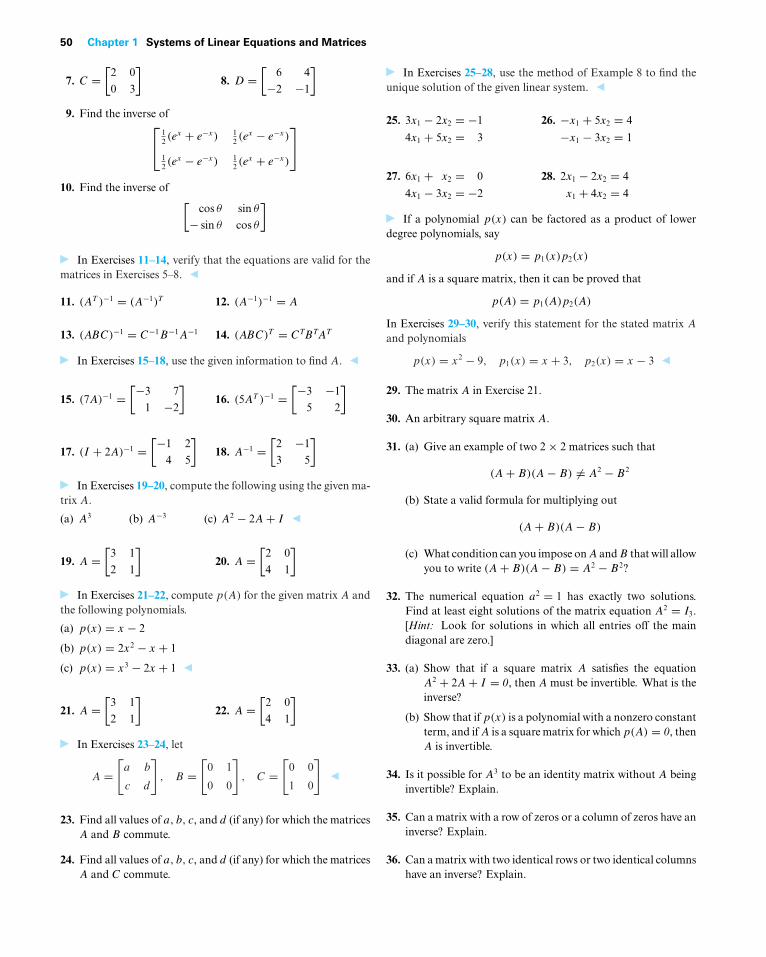
50 Chapter 1 Systems of Linear Equations and Matrices
7. C =[
2 0
0 3
]8. D =
[6 4
−2 −1
]
9. Find the inverse of⎡⎣ 1
2 (ex + e−x) 1
2 (ex − e−x)
12 (e
x − e−x) 12 (e
x + e−x)
⎤⎦
10. Find the inverse of [cos θ sin θ
− sin θ cos θ
]
In Exercises 11–14, verify that the equations are valid for thematrices in Exercises 5–8.
11. (AT )−1 = (A−1)T 12. (A−1)−1 = A
13. (ABC)−1 = C−1B−1A−1 14. (ABC)T = CTBTAT
In Exercises 15–18, use the given information to find A.
15. (7A)−1 =[−3 7
1 −2
]16. (5AT )−1 =
[−3 −1
5 2
]
17. (I + 2A)−1 =[−1 2
4 5
]18. A−1 =
[2 −1
3 5
]
In Exercises 19–20, compute the following using the given ma-trix A.
(a) A3 (b) A−3 (c) A2 − 2A + I
19. A =[
3 1
2 1
]20. A =
[2 0
4 1
]
In Exercises 21–22, compute p(A) for the given matrix A andthe following polynomials.
(a) p(x) = x − 2
(b) p(x) = 2x2 − x + 1
(c) p(x) = x3 − 2x + 1
21. A =[
3 1
2 1
]22. A =
[2 0
4 1
]
In Exercises 23–24, let
A =[a b
c d
], B =
[0 1
0 0
], C =
[0 0
1 0
]
23. Find all values of a, b, c, and d (if any) for which the matricesA and B commute.
24. Find all values of a, b, c, and d (if any) for which the matricesA and C commute.
In Exercises 25–28, use the method of Example 8 to find theunique solution of the given linear system.
25. 3x1 − 2x2 = −1
4x1 + 5x2 = 3
26. −x1 + 5x2 = 4
−x1 − 3x2 = 1
27. 6x1 + x2 = 0
4x1 − 3x2 = −2
28. 2x1 − 2x2 = 4
x1 + 4x2 = 4
If a polynomial p(x) can be factored as a product of lowerdegree polynomials, say
p(x) = p1(x)p2(x)
and if A is a square matrix, then it can be proved that
p(A) = p1(A)p2(A)
In Exercises 29–30, verify this statement for the stated matrix A
and polynomials
p(x) = x2 − 9, p1(x) = x + 3, p2(x) = x − 3
29. The matrix A in Exercise 21.
30. An arbitrary square matrix A.
31. (a) Give an example of two 2 × 2 matrices such that
(A + B)(A − B) �= A2 − B2
(b) State a valid formula for multiplying out
(A + B)(A − B)
(c) What condition can you impose on A and B that will allowyou to write (A + B)(A − B) = A2 − B2?
32. The numerical equation a2 = 1 has exactly two solutions.Find at least eight solutions of the matrix equation A2 = I3.[Hint: Look for solutions in which all entries off the maindiagonal are zero.]
33. (a) Show that if a square matrix A satisfies the equationA2 + 2A + I = 0, then A must be invertible. What is theinverse?
(b) Show that if p(x) is a polynomial with a nonzero constantterm, and if A is a square matrix for which p(A) = 0, thenA is invertible.
34. Is it possible for A3 to be an identity matrix without A beinginvertible? Explain.
35. Can a matrix with a row of zeros or a column of zeros have aninverse? Explain.
36. Can a matrix with two identical rows or two identical columnshave an inverse? Explain.
1.4 Inverses; Algebraic Properties of Matrices 51
In Exercises 37–38, determine whether A is invertible, and ifso, find the inverse. [Hint: Solve AX = I for X by equating cor-responding entries on the two sides.]
37. A =⎡⎢⎣1 0 1
1 1 0
0 1 1
⎤⎥⎦ 38. A =
⎡⎢⎣1 1 1
1 0 0
0 1 1
⎤⎥⎦
In Exercises 39–40, simplify the expression assuming that A,B, C, and D are invertible.
39. (AB)−1(AC−1)(D−1C−1)−1D−1
40. (AC−1)−1(AC−1)(AC−1)−1AD−1
41. Show that if R is a 1 × n matrix and C is an n × 1 matrix,then RC = tr(CR).
42. If A is a square matrix and n is a positive integer, is it true that(An)T = (AT )n? Justify your answer.
43. (a) Show that if A is invertible and AB = AC, then B = C.
(b) Explain why part (a) and Example 3 do not contradict oneanother.
44. Show that if A is invertible and k is any nonzero scalar, then(kA)n = knAn for all integer values of n.
45. (a) Show that if A, B, and A + B are invertible matrices withthe same size, then
A(A−1 + B−1)B(A + B)−1 = I
(b) What does the result in part (a) tell you about the matrixA−1 + B−1?
46. A square matrix A is said to be idempotent if A2 = A.
(a) Show that if A is idempotent, then so is I − A.
(b) Show that if A is idempotent, then 2A − I is invertibleand is its own inverse.
47. Show that if A is a square matrix such that Ak = 0 for somepositive integer k, then the matrix I − A is invertible and
(I − A)−1 = I + A + A2 + · · · + Ak−1
48. Show that the matrix
A =[a b
c d
]
satisfies the equation
A2 − (a + d)A + (ad − bc)I = 0
49. Assuming that all matrices are n × n and invertible, solvefor D.
CT B−1A2BAC−1DA−2BT C−2 = CT
50. Assuming that all matrices are n × n and invertible, solvefor D.
ABCTDBAT C = ABT
Working with Proofs
In Exercises 51–58, prove the stated result.
51. Theorem 1.4.1(a) 52. Theorem 1.4.1(b)
53. Theorem 1.4.1( f ) 54. Theorem 1.4.1(c)
55. Theorem 1.4.2(c) 56. Theorem 1.4.2(b)
57. Theorem 1.4.8(d) 58. Theorem 1.4.8(e)
True-False Exercises
TF. In parts (a)–(k) determine whether the statement is true orfalse, and justify your answer.
(a) Two n × n matrices, A and B, are inverses of one another ifand only if AB = BA = 0.
(b) For all square matrices A and B of the same size, it is true that(A + B)2 = A2 + 2AB + B2.
(c) For all square matrices A and B of the same size, it is true thatA2 − B2 = (A − B)(A + B).
(d) If A and B are invertible matrices of the same size, then AB isinvertible and (AB)−1 = A−1B−1.
(e) If A and B are matrices such that AB is defined, then it is truethat (AB)T = ATBT .
(f ) The matrix
A =[a b
c d
]is invertible if and only if ad − bc �= 0.
(g) If A and B are matrices of the same size and k is a constant,then (kA + B)T = kAT + BT .
(h) If A is an invertible matrix, then so is AT .
(i) If p(x) = a0 + a1x + a2x2 + · · · + amxm and I is an identity
matrix, then p(I) = a0 + a1 + a2 + · · · + am.
( j) A square matrix containing a row or column of zeros cannotbe invertible.
(k) The sum of two invertible matrices of the same size must beinvertible.
52 Chapter 1 Systems of Linear Equations and Matrices
Working withTechnology
T1. Let A be the matrix
A =
⎡⎢⎢⎣
0 12
13
14 0 1
5
16
17 0
⎤⎥⎥⎦
Discuss the behavior of Ak as k increases indefinitely, that is, ask→�.
T2. In each part use your technology utility to make a conjectureabout the form of An for positive integer powers of n.
(a) A =[a 1
0 a
](b) A =
[cos θ sin θ
− sin θ cos θ
]
T3. The Fibonacci sequence (named for the Italian mathematicianLeonardo Fibonacci 1170–1250) is
0, 1, 1, 2, 3, 5, 8, 13, 21, 34, 55, 89, 144, . . .
the terms of which are commonly denoted as
F0, F1, F2, F3, . . . , Fn, . . .
After the initial terms F0 = 0 and F1 = 1, each term is the sum ofthe previous two; that is,
Fn = Fn−1 + Fn−2
Confirm that if
Q =[F2 F1
F1 F0
]=[
1 1
1 0
]
then
Qn =[Fn+1 Fn
Fn F0
]
1.5 Elementary Matrices and a Method for FindingA−1
In this section we will develop an algorithm for finding the inverse of a matrix, and we willdiscuss some of the basic properties of invertible matrices.
In Section 1.1 we defined three elementary row operations on a matrix A:
1. Multiply a row by a nonzero constant c.
2. Interchange two rows.
3. Add a constant c times one row to another.
It should be evident that if we let B be the matrix that results from A by performing oneof the operations in this list, then the matrix A can be recovered from B by performingthe corresponding operation in the following list:
1. Multiply the same row by 1/c.
2. Interchange the same two rows.
3. If B resulted by adding c times row ri of A to row rj , then add −c times rj to ri .
It follows that if B is obtained from A by performing a sequence of elementary rowoperations, then there is a second sequence of elementary row operations, which whenapplied to B recovers A (Exercise 33). Accordingly, we make the following definition.
DEFINITION 1 Matrices A and B are said to be row equivalent if either (hence each)can be obtained from the other by a sequence of elementary row operations.
Our next goal is to show how matrix multiplication can be used to carry out anelementary row operation.
DEFINITION 2 A matrix E is called an elementary matrix if it can be obtained froman identity matrix by performing a single elementary row operation.
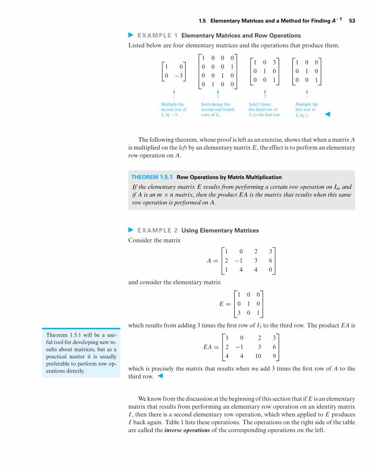
1.5 Elementary Matrices and a Method for FindingA−1 53
EXAMPLE 1 Elementary Matrices and Row Operations
Listed below are four elementary matrices and the operations that produce them.
[1 0
0 −3
] ⎡⎢⎢⎢⎣
1 0 0 00 0 0 10 0 1 00 1 0 0
⎤⎥⎥⎥⎦
⎡⎢⎣1 0 3
0 1 00 0 1
⎤⎥⎦
⎡⎢⎣1 0 0
0 1 00 0 1
⎤⎥⎦
�
Multiply thesecond row ofI2 by −3.
�
Interchange thesecond and fourthrows of I4.
�Add 3 timesthe third row ofI3 to the first row.
�
Multiply thefirst row ofI3 by 1.
The following theorem, whose proof is left as an exercise, shows that when a matrix A
is multiplied on the left by an elementary matrix E, the effect is to perform an elementaryrow operation on A.
THEOREM 1.5.1 Row Operations by Matrix Multiplication
If the elementary matrix E results from performing a certain row operation on Im andif A is an m × n matrix, then the product EA is the matrix that results when this samerow operation is performed on A.
EXAMPLE 2 Using Elementary Matrices
Consider the matrix
A =⎡⎢⎣1 0 2 3
2 −1 3 6
1 4 4 0
⎤⎥⎦
and consider the elementary matrix
E =⎡⎢⎣1 0 0
0 1 0
3 0 1
⎤⎥⎦
which results from adding 3 times the first row of I3 to the third row. The product EA is
Theorem 1.5.1 will be a use-ful tool for developing new re-sults about matrices, but as apractical matter it is usuallypreferable to perform row op-erations directly.
EA =⎡⎢⎣1 0 2 3
2 −1 3 6
4 4 10 9
⎤⎥⎦
which is precisely the matrix that results when we add 3 times the first row of A to thethird row.
We know from the discussion at the beginning of this section that if E is an elementarymatrix that results from performing an elementary row operation on an identity matrixI , then there is a second elementary row operation, which when applied to E producesI back again. Table 1 lists these operations. The operations on the right side of the tableare called the inverse operations of the corresponding operations on the left.
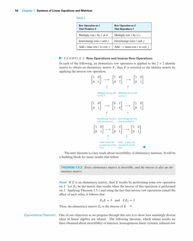
54 Chapter 1 Systems of Linear Equations and Matrices
Table 1
Row Operation on I Row Operation on EThat Produces E That Reproduces I
Multiply row i by c �= 0 Multiply row i by 1/c
Interchange rows i and j Interchange rows i and j
Add c time row i to row j Add −c times row i to row j
EXAMPLE 3 Row Operations and Inverse Row Operations
In each of the following, an elementary row operation is applied to the 2 × 2 identitymatrix to obtain an elementary matrix E, then E is restored to the identity matrix byapplying the inverse row operation.[
1 00 1
]−→
[1 00 7
]−→
[1 00 1
]�
Multiply the secondrow by 7.
�
Multiply the secondrow by 1
7 .[1 00 1
]−→
[0 11 0
]−→
[1 00 1
]
�
Interchange the firstand second rows.
�
Interchange the firstand second rows.[
1 00 1
]−→
[1 50 1
]−→
[1 00 1
]
�
Add 5 times thesecond row to thefirst.
�
Add −5 times thesecond row to thefirst.
The next theorem is a key result about invertibility of elementary matrices. It will bea building block for many results that follow.
THEOREM 1.5.2 Every elementary matrix is invertible, and the inverse is also an ele-mentary matrix.
Proof If E is an elementary matrix, then E results by performing some row operationon I . Let E0 be the matrix that results when the inverse of this operation is performedon I . Applying Theorem 1.5.1 and using the fact that inverse row operations cancel theeffect of each other, it follows that
E0E = I and EE0 = I
Thus, the elementary matrix E0 is the inverse of E.
EquivalenceTheorem One of our objectives as we progress through this text is to show how seemingly diverseideas in linear algebra are related. The following theorem, which relates results wehave obtained about invertibility of matrices, homogeneous linear systems, reduced row
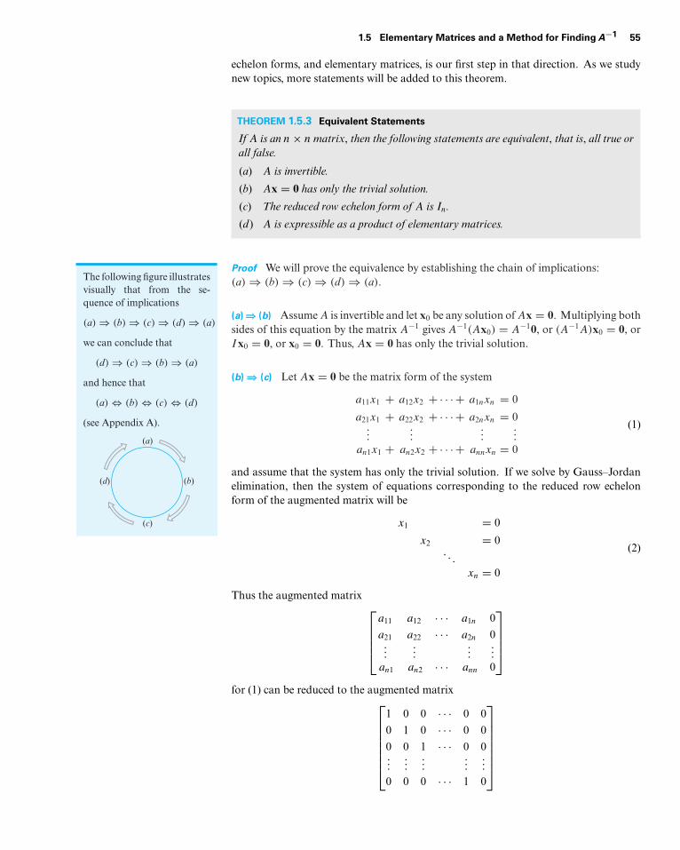
1.5 Elementary Matrices and a Method for FindingA−1 55
echelon forms, and elementary matrices, is our first step in that direction. As we studynew topics, more statements will be added to this theorem.
THEOREM 1.5.3 Equivalent Statements
IfA is an n × nmatrix, then the following statements are equivalent, that is, all true orall false.
(a) A is invertible.
(b) Ax = 0 has only the trivial solution.
(c) The reduced row echelon form of A is In.
(d ) A is expressible as a product of elementary matrices.
Proof We will prove the equivalence by establishing the chain of implications:The following figure illustratesvisually that from the se-quence of implications
(a) ⇒ (b) ⇒ (c) ⇒ (d) ⇒ (a)
we can conclude that
(d) ⇒ (c) ⇒ (b) ⇒ (a)
and hence that
(a) ⇔ (b) ⇔ (c) ⇔ (d)
(see Appendix A).
(a)
(c)
(d) (b)
(a) ⇒ (b) ⇒ (c) ⇒ (d) ⇒ (a).
(a)⇒ (b) Assume A is invertible and let x0 be any solution of Ax = 0. Multiplying bothsides of this equation by the matrix A−1 gives A−1(Ax0) = A−10, or (A−1A)x0 = 0, orIx0 = 0, or x0 = 0. Thus, Ax = 0 has only the trivial solution.
(b) ⇒ (c) Let Ax = 0 be the matrix form of the system
a11x1 + a12x2 + · · ·+ a1nxn = 0
a21x1 + a22x2 + · · ·+ a2nxn = 0...
......
...an1x1 + an2x2 + · · ·+ annxn = 0
(1)
and assume that the system has only the trivial solution. If we solve by Gauss–Jordanelimination, then the system of equations corresponding to the reduced row echelonform of the augmented matrix will be
x1 = 0
x2 = 0. . .
xn = 0
(2)
Thus the augmented matrix ⎡⎢⎢⎢⎣
a11 a12 · · · a1n 0
a21 a22 · · · a2n 0...
......
...an1 an2 · · · ann 0
⎤⎥⎥⎥⎦
for (1) can be reduced to the augmented matrix⎡⎢⎢⎢⎢⎢⎢⎣
1 0 0 · · · 0 0
0 1 0 · · · 0 0
0 0 1 · · · 0 0...
......
......
0 0 0 · · · 1 0
⎤⎥⎥⎥⎥⎥⎥⎦
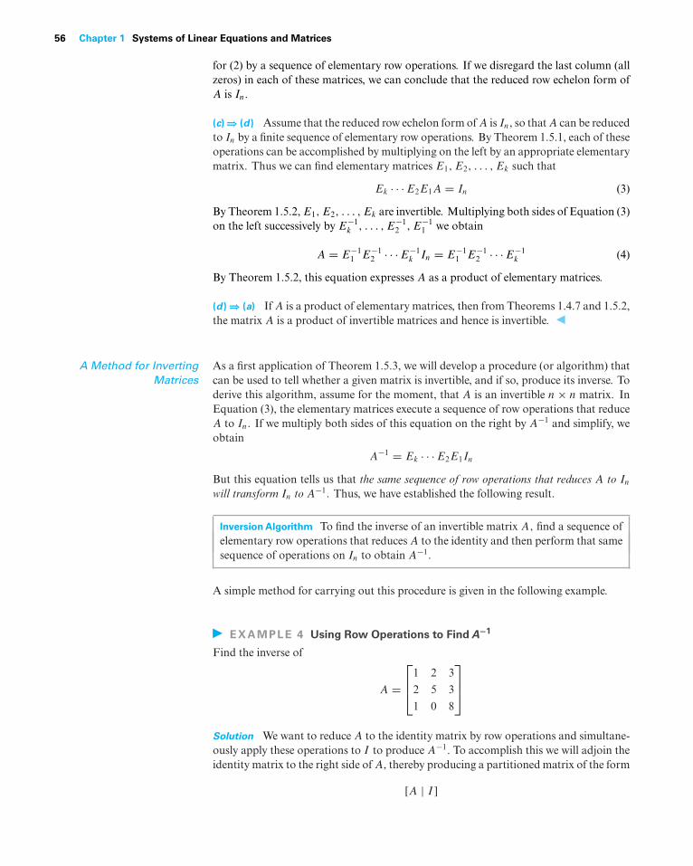
56 Chapter 1 Systems of Linear Equations and Matrices
for (2) by a sequence of elementary row operations. If we disregard the last column (allzeros) in each of these matrices, we can conclude that the reduced row echelon form ofA is In.
(c)⇒ (d ) Assume that the reduced row echelon form of A is In, so that A can be reducedto In by a finite sequence of elementary row operations. By Theorem 1.5.1, each of theseoperations can be accomplished by multiplying on the left by an appropriate elementarymatrix. Thus we can find elementary matrices E1, E2, . . . , Ek such that
Ek · · ·E2E1A = In (3)
By Theorem 1.5.2, E1, E2, . . . , Ek are invertible. Multiplying both sides of Equation (3)on the left successively by E−1
k , . . . , E−12 , E−1
1 we obtain
A = E−11 E−1
2 · · ·E−1k In = E−1
1 E−12 · · ·E−1
k (4)
By Theorem 1.5.2, this equation expresses A as a product of elementary matrices.
(d ) ⇒ (a) If A is a product of elementary matrices, then from Theorems 1.4.7 and 1.5.2,the matrix A is a product of invertible matrices and hence is invertible.
A Method for InvertingMatrices
As a first application of Theorem 1.5.3, we will develop a procedure (or algorithm) thatcan be used to tell whether a given matrix is invertible, and if so, produce its inverse. Toderive this algorithm, assume for the moment, that A is an invertible n × n matrix. InEquation (3), the elementary matrices execute a sequence of row operations that reduceA to In. If we multiply both sides of this equation on the right by A−1 and simplify, weobtain
A−1 = Ek · · ·E2E1In
But this equation tells us that the same sequence of row operations that reduces A to In
will transform In to A−1. Thus, we have established the following result.
Inversion Algorithm To find the inverse of an invertible matrix A, find a sequence ofelementary row operations that reduces A to the identity and then perform that samesequence of operations on In to obtain A−1.
A simple method for carrying out this procedure is given in the following example.
EXAMPLE 4 Using Row Operations to FindA−1
Find the inverse of
A =⎡⎢⎣1 2 3
2 5 3
1 0 8
⎤⎥⎦
Solution We want to reduce A to the identity matrix by row operations and simultane-ously apply these operations to I to produce A−1. To accomplish this we will adjoin theidentity matrix to the right side of A, thereby producing a partitioned matrix of the form
[A | I ]
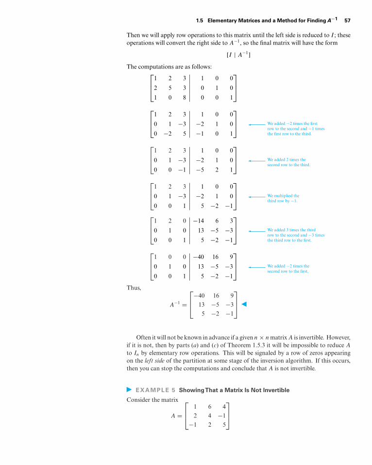
1.5 Elementary Matrices and a Method for FindingA−1 57
Then we will apply row operations to this matrix until the left side is reduced to I ; theseoperations will convert the right side to A−1, so the final matrix will have the form
[I | A−1]The computations are as follows:⎡
⎢⎣1 2 3 1 0 0
2 5 3 0 1 0
1 0 8 0 0 1
⎤⎥⎦
⎡⎢⎣1 2 3 1 0 0
0 1 −3 −2 1 0
0 −2 5 −1 0 1
⎤⎥⎦ We added −2 times the first
row to the second and −1 timesthe first row to the third.
⎡⎢⎣1 2 3 1 0 0
0 1 −3 −2 1 0
0 0 −1 −5 2 1
⎤⎥⎦ We added 2 times the
second row to the third.
⎡⎢⎣1 2 3 1 0 0
0 1 −3 −2 1 0
0 0 1 5 −2 −1
⎤⎥⎦ We multiplied the
third row by −1.
⎡⎢⎣1 2 0 −14 6 3
0 1 0 13 −5 −3
0 0 1 5 −2 −1
⎤⎥⎦ We added 3 times the third
row to the second and −3 timesthe third row to the first.
⎡⎢⎣1 0 0 −40 16 9
0 1 0 13 −5 −3
0 0 1 5 −2 −1
⎤⎥⎦ We added −2 times the
second row to the first.
Thus,
A−1 =⎡⎢⎣−40 16 9
13 −5 −3
5 −2 −1
⎤⎥⎦
Often it will not be known in advance if a given n × n matrix A is invertible. However,if it is not, then by parts (a) and (c) of Theorem 1.5.3 it will be impossible to reduce A
to In by elementary row operations. This will be signaled by a row of zeros appearingon the left side of the partition at some stage of the inversion algorithm. If this occurs,then you can stop the computations and conclude that A is not invertible.
EXAMPLE 5 ShowingThat a Matrix Is Not Invertible
Consider the matrix
A =⎡⎢⎣ 1 6 4
2 4 −1
−1 2 5
⎤⎥⎦
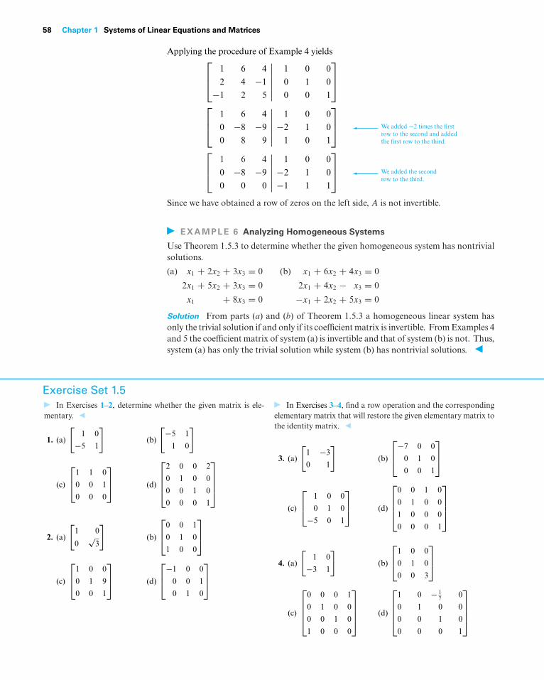
58 Chapter 1 Systems of Linear Equations and Matrices
Applying the procedure of Example 4 yields⎡⎢⎣ 1 6 4 1 0 0
2 4 −1 0 1 0
−1 2 5 0 0 1
⎤⎥⎦
⎡⎢⎣ 1 6 4 1 0 0
0 −8 −9 −2 1 0
0 8 9 1 0 1
⎤⎥⎦ We added −2 times the first
row to the second and addedthe first row to the third.⎡
⎢⎣ 1 6 4 1 0 0
0 −8 −9 −2 1 0
0 0 0 −1 1 1
⎤⎥⎦ We added the second
row to the third.
Since we have obtained a row of zeros on the left side, A is not invertible.
EXAMPLE 6 Analyzing Homogeneous Systems
Use Theorem 1.5.3 to determine whether the given homogeneous system has nontrivialsolutions.
(a) x1 + 2x2 + 3x3 = 0
2x1 + 5x2 + 3x3 = 0
x1 + 8x3 = 0
(b) x1 + 6x2 + 4x3 = 0
2x1 + 4x2 − x3 = 0
−x1 + 2x2 + 5x3 = 0
Solution From parts (a) and (b) of Theorem 1.5.3 a homogeneous linear system hasonly the trivial solution if and only if its coefficient matrix is invertible. From Examples 4and 5 the coefficient matrix of system (a) is invertible and that of system (b) is not. Thus,system (a) has only the trivial solution while system (b) has nontrivial solutions.
Exercise Set 1.5In Exercises 1–2, determine whether the given matrix is ele-
mentary.
1. (a)
[1 0
−5 1
](b)
[−5 1
1 0
]
(c)
⎡⎢⎣1 1 0
0 0 1
0 0 0
⎤⎥⎦ (d)
⎡⎢⎢⎢⎣
2 0 0 2
0 1 0 0
0 0 1 0
0 0 0 1
⎤⎥⎥⎥⎦
2. (a)
[1 0
0√
3
](b)
⎡⎢⎣0 0 1
0 1 0
1 0 0
⎤⎥⎦
(c)
⎡⎢⎣1 0 0
0 1 9
0 0 1
⎤⎥⎦ (d)
⎡⎢⎣−1 0 0
0 0 1
0 1 0
⎤⎥⎦
In Exercises 3–4, find a row operation and the correspondingelementary matrix that will restore the given elementary matrix tothe identity matrix.
3. (a)
[1 −3
0 1
](b)
⎡⎢⎣−7 0 0
0 1 0
0 0 1
⎤⎥⎦
(c)
⎡⎢⎣ 1 0 0
0 1 0
−5 0 1
⎤⎥⎦ (d)
⎡⎢⎢⎢⎣
0 0 1 0
0 1 0 0
1 0 0 0
0 0 0 1
⎤⎥⎥⎥⎦
4. (a)
[1 0
−3 1
](b)
⎡⎢⎣1 0 0
0 1 0
0 0 3
⎤⎥⎦
(c)
⎡⎢⎢⎢⎣
0 0 0 1
0 1 0 0
0 0 1 0
1 0 0 0
⎤⎥⎥⎥⎦ (d)
⎡⎢⎢⎢⎣
1 0 − 17 0
0 1 0 0
0 0 1 0
0 0 0 1
⎤⎥⎥⎥⎦
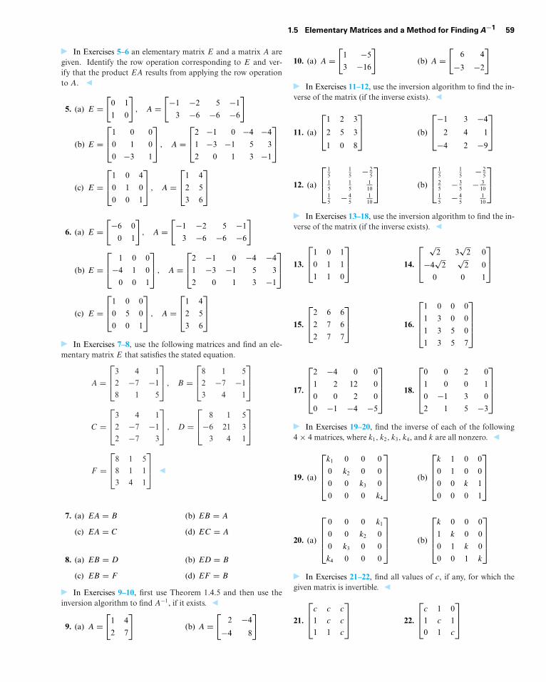
1.5 Elementary Matrices and a Method for FindingA−1 59
In Exercises 5–6 an elementary matrix E and a matrix A aregiven. Identify the row operation corresponding to E and ver-ify that the product EA results from applying the row operationto A.
5. (a) E =[
0 1
1 0
], A =
[−1 −2 5 −1
3 −6 −6 −6
]
(b) E =⎡⎢⎣1 0 0
0 1 0
0 −3 1
⎤⎥⎦ , A =
⎡⎢⎣2 −1 0 −4 −4
1 −3 −1 5 3
2 0 1 3 −1
⎤⎥⎦
(c) E =⎡⎢⎣1 0 4
0 1 0
0 0 1
⎤⎥⎦ , A =
⎡⎢⎣1 4
2 5
3 6
⎤⎥⎦
6. (a) E =[−6 0
0 1
], A =
[−1 −2 5 −1
3 −6 −6 −6
]
(b) E =⎡⎢⎣ 1 0 0
−4 1 0
0 0 1
⎤⎥⎦ , A =
⎡⎢⎣2 −1 0 −4 −4
1 −3 −1 5 3
2 0 1 3 −1
⎤⎥⎦
(c) E =⎡⎢⎣1 0 0
0 5 0
0 0 1
⎤⎥⎦ , A =
⎡⎢⎣1 4
2 5
3 6
⎤⎥⎦
In Exercises 7–8, use the following matrices and find an ele-mentary matrix E that satisfies the stated equation.
A =⎡⎢⎣3 4 1
2 −7 −1
8 1 5
⎤⎥⎦ , B =
⎡⎢⎣8 1 5
2 −7 −1
3 4 1
⎤⎥⎦
C =⎡⎢⎣3 4 1
2 −7 −1
2 −7 3
⎤⎥⎦ , D =
⎡⎢⎣ 8 1 5
−6 21 3
3 4 1
⎤⎥⎦
F =⎡⎢⎣8 1 5
8 1 1
3 4 1
⎤⎥⎦
7. (a) EA = B (b) EB = A
(c) EA = C (d) EC = A
8. (a) EB = D (b) ED = B
(c) EB = F (d) EF = B
In Exercises 9–10, first use Theorem 1.4.5 and then use theinversion algorithm to find A−1, if it exists.
9. (a) A =[
1 4
2 7
](b) A =
[2 −4
−4 8
]
10. (a) A =[
1 −5
3 −16
](b) A =
[6 4
−3 −2
]
In Exercises 11–12, use the inversion algorithm to find the in-verse of the matrix (if the inverse exists).
11. (a)
⎡⎢⎣
1 2 3
2 5 3
1 0 8
⎤⎥⎦ (b)
⎡⎢⎣−1 3 −4
2 4 1
−4 2 −9
⎤⎥⎦
12. (a)
⎡⎢⎣
15
15 − 2
515
15
110
15 − 4
5110
⎤⎥⎦ (b)
⎡⎢⎣
15
15 − 2
525 − 3
5 − 310
15 − 4
5110
⎤⎥⎦
In Exercises 13–18, use the inversion algorithm to find the in-verse of the matrix (if the inverse exists).
13.
⎡⎢⎣1 0 1
0 1 1
1 1 0
⎤⎥⎦ 14.
⎡⎢⎣
√2 3
√2 0
−4√
2√
2 0
0 0 1
⎤⎥⎦
15.
⎡⎢⎣2 6 6
2 7 6
2 7 7
⎤⎥⎦ 16.
⎡⎢⎢⎢⎣
1 0 0 0
1 3 0 0
1 3 5 0
1 3 5 7
⎤⎥⎥⎥⎦
17.
⎡⎢⎢⎢⎣
2 −4 0 0
1 2 12 0
0 0 2 0
0 −1 −4 −5
⎤⎥⎥⎥⎦ 18.
⎡⎢⎢⎢⎣
0 0 2 0
1 0 0 1
0 −1 3 0
2 1 5 −3
⎤⎥⎥⎥⎦
In Exercises 19–20, find the inverse of each of the following4 × 4 matrices, where k1, k2, k3, k4, and k are all nonzero.
19. (a)
⎡⎢⎢⎢⎣
k1 0 0 0
0 k2 0 0
0 0 k3 0
0 0 0 k4
⎤⎥⎥⎥⎦ (b)
⎡⎢⎢⎢⎣
k 1 0 0
0 1 0 0
0 0 k 1
0 0 0 1
⎤⎥⎥⎥⎦
20. (a)
⎡⎢⎢⎢⎣
0 0 0 k1
0 0 k2 0
0 k3 0 0
k4 0 0 0
⎤⎥⎥⎥⎦ (b)
⎡⎢⎢⎢⎣
k 0 0 0
1 k 0 0
0 1 k 0
0 0 1 k
⎤⎥⎥⎥⎦
In Exercises 21–22, find all values of c, if any, for which thegiven matrix is invertible.
21.
⎡⎢⎣c c c
1 c c
1 1 c
⎤⎥⎦ 22.
⎡⎢⎣c 1 0
1 c 1
0 1 c
⎤⎥⎦
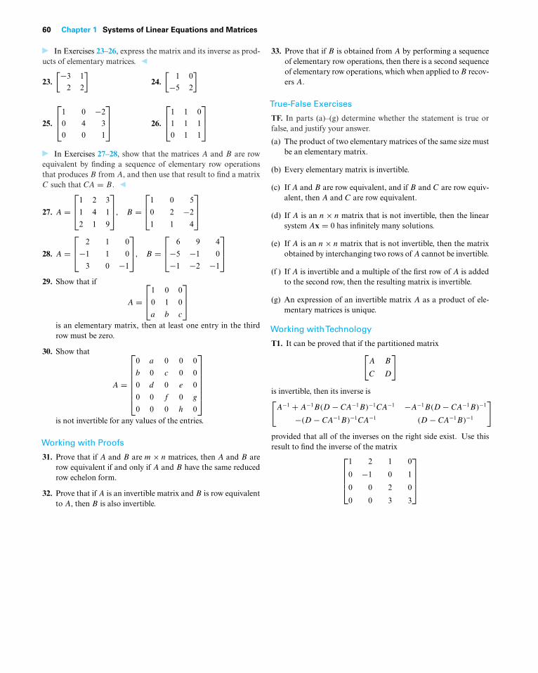
60 Chapter 1 Systems of Linear Equations and Matrices
In Exercises 23–26, express the matrix and its inverse as prod-ucts of elementary matrices.
23.[−3 1
2 2
]24.
[1 0
−5 2
]
25.
⎡⎢⎣1 0 −2
0 4 3
0 0 1
⎤⎥⎦ 26.
⎡⎢⎣1 1 0
1 1 1
0 1 1
⎤⎥⎦
In Exercises 27–28, show that the matrices A and B are rowequivalent by finding a sequence of elementary row operationsthat produces B from A, and then use that result to find a matrixC such that CA = B.
27. A =⎡⎢⎣1 2 3
1 4 1
2 1 9
⎤⎥⎦, B =
⎡⎢⎣1 0 5
0 2 −2
1 1 4
⎤⎥⎦
28. A =⎡⎢⎣ 2 1 0
−1 1 0
3 0 −1
⎤⎥⎦, B =
⎡⎢⎣ 6 9 4
−5 −1 0
−1 −2 −1
⎤⎥⎦
29. Show that if
A =⎡⎢⎣1 0 0
0 1 0
a b c
⎤⎥⎦
is an elementary matrix, then at least one entry in the thirdrow must be zero.
30. Show that
A =
⎡⎢⎢⎢⎢⎢⎢⎣
0 a 0 0 0
b 0 c 0 0
0 d 0 e 0
0 0 f 0 g
0 0 0 h 0
⎤⎥⎥⎥⎥⎥⎥⎦
is not invertible for any values of the entries.
Working with Proofs
31. Prove that if A and B are m × n matrices, then A and B arerow equivalent if and only if A and B have the same reducedrow echelon form.
32. Prove that if A is an invertible matrix and B is row equivalentto A, then B is also invertible.
33. Prove that if B is obtained from A by performing a sequenceof elementary row operations, then there is a second sequenceof elementary row operations, which when applied to B recov-ers A.
True-False Exercises
TF. In parts (a)–(g) determine whether the statement is true orfalse, and justify your answer.
(a) The product of two elementary matrices of the same size mustbe an elementary matrix.
(b) Every elementary matrix is invertible.
(c) If A and B are row equivalent, and if B and C are row equiv-alent, then A and C are row equivalent.
(d) If A is an n × n matrix that is not invertible, then the linearsystem Ax = 0 has infinitely many solutions.
(e) If A is an n × n matrix that is not invertible, then the matrixobtained by interchanging two rows of A cannot be invertible.
(f ) If A is invertible and a multiple of the first row of A is addedto the second row, then the resulting matrix is invertible.
(g) An expression of an invertible matrix A as a product of ele-mentary matrices is unique.
Working withTechnology
T1. It can be proved that if the partitioned matrix[A B
C D
]
is invertible, then its inverse is[A−1 + A−1B(D − CA−1B)−1CA−1 −A−1B(D − CA−1B)−1
−(D − CA−1B)−1CA−1 (D − CA−1B)−1
]
provided that all of the inverses on the right side exist. Use thisresult to find the inverse of the matrix⎡
⎢⎢⎢⎣1 2 1 0
0 −1 0 1
0 0 2 0
0 0 3 3
⎤⎥⎥⎥⎦
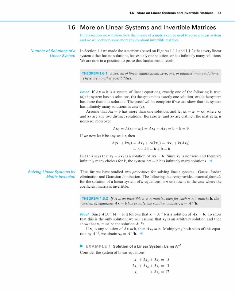
1.6 More on Linear Systems and Invertible Matrices 61
1.6 More on Linear Systems and Invertible MatricesIn this section we will show how the inverse of a matrix can be used to solve a linear systemand we will develop some more results about invertible matrices.
Number of Solutions of aLinear System
In Section 1.1 we made the statement (based on Figures 1.1.1 and 1.1.2) that every linearsystem either has no solutions, has exactly one solution, or has infinitely many solutions.We are now in a position to prove this fundamental result.
THEOREM1.6.1 A system of linear equations has zero, one, or infinitelymany solutions.There are no other possibilities.
Proof If Ax = b is a system of linear equations, exactly one of the following is true:(a) the system has no solutions, (b) the system has exactly one solution, or (c) the systemhas more than one solution. The proof will be complete if we can show that the systemhas infinitely many solutions in case (c).
Assume that Ax = b has more than one solution, and let x0 = x1 − x2, where x1
and x2 are any two distinct solutions. Because x1 and x2 are distinct, the matrix x0 isnonzero; moreover,
Ax0 = A(x1 − x2) = Ax1 − Ax2 = b − b = 0
If we now let k be any scalar, then
A(x1 + kx0) = Ax1 + A(kx0) = Ax1 + k(Ax0)
= b + k0 = b + 0 = b
But this says that x1 + kx0 is a solution of Ax = b. Since x0 is nonzero and there areinfinitely many choices for k, the system Ax = b has infinitely many solutions.
Solving Linear Systems byMatrix Inversion
Thus far we have studied two procedures for solving linear systems—Gauss–Jordanelimination and Gaussian elimination. The following theorem provides an actual formulafor the solution of a linear system of n equations in n unknowns in the case where thecoefficient matrix is invertible.
THEOREM 1.6.2 If A is an invertible n × n matrix, then for each n × 1 matrix b, thesystem of equations Ax = b has exactly one solution, namely, x = A−1b.
Proof Since A(A−1b) = b, it follows that x = A−1b is a solution of Ax = b. To showthat this is the only solution, we will assume that x0 is an arbitrary solution and thenshow that x0 must be the solution A−1b.
If x0 is any solution of Ax = b, then Ax0 = b. Multiplying both sides of this equa-tion by A−1, we obtain x0 = A−1b.
EXAMPLE 1 Solution of a Linear System UsingA−1
Consider the system of linear equations
x1 + 2x2 + 3x3 = 5
2x1 + 5x2 + 3x3 = 3
x1 + 8x3 = 17
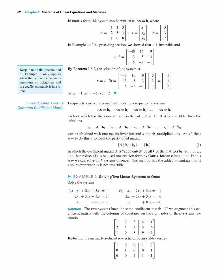
62 Chapter 1 Systems of Linear Equations and Matrices
In matrix form this system can be written as Ax = b, where
A =⎡⎢⎣1 2 3
2 5 3
1 0 8
⎤⎥⎦, x =
⎡⎢⎣x1
x2
x3
⎤⎥⎦, b =
⎡⎢⎣ 5
3
17
⎤⎥⎦
In Example 4 of the preceding section, we showed that A is invertible and
A−1 =⎡⎢⎣−40 16 9
13 −5 −3
5 −2 −1
⎤⎥⎦
By Theorem 1.6.2, the solution of the system isKeep in mind that the methodof Example 1 only applieswhen the system has as manyequations as unknowns andthe coefficient matrix is invert-ible.
x = A−1b =⎡⎢⎣−40 16 9
13 −5 −3
5 −2 −1
⎤⎥⎦⎡⎢⎣ 5
3
17
⎤⎥⎦ =
⎡⎢⎣ 1
−1
2
⎤⎥⎦
or x1 = 1, x2 = −1, x3 = 2.
Linear Systems with aCommon Coefficient Matrix
Frequently, one is concerned with solving a sequence of systems
Ax = b1, Ax = b2, Ax = b3, . . . , Ax = bk
each of which has the same square coefficient matrix A. If A is invertible, then thesolutions
x1 = A−1b1, x2 = A−1b2, x3 = A−1b3, . . . , xk = A−1bk
can be obtained with one matrix inversion and k matrix multiplications. An efficientway to do this is to form the partitioned matrix
[A | b1 | b2 | · · · | bk] (1)
in which the coefficient matrix A is “augmented” by all k of the matrices b1, b2, . . . , bk ,and then reduce (1) to reduced row echelon form by Gauss–Jordan elimination. In thisway we can solve all k systems at once. This method has the added advantage that itapplies even when A is not invertible.
EXAMPLE 2 SolvingTwo Linear Systems at Once
Solve the systems
(a) x1 + 2x2 + 3x3 = 4
2x1 + 5x2 + 3x3 = 5
x1 + 8x3 = 9
(b) x1 + 2x2 + 3x3 = 1
2x1 + 5x2 + 3x3 = 6
x1 + 8x3 = −6
Solution The two systems have the same coefficient matrix. If we augment this co-efficient matrix with the columns of constants on the right sides of these systems, weobtain ⎡
⎢⎣1 2 3 4 1
2 5 3 5 6
1 0 8 9 −6
⎤⎥⎦
Reducing this matrix to reduced row echelon form yields (verify)⎡⎢⎣1 0 0 1 2
0 1 0 0 1
0 0 1 1 −1
⎤⎥⎦
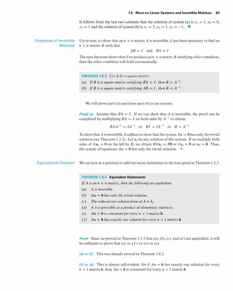
1.6 More on Linear Systems and Invertible Matrices 63
It follows from the last two columns that the solution of system (a) is x1 = 1, x2 = 0,x3 = 1 and the solution of system (b) is x1 = 2, x2 = 1, x3 = −1.
Properties of InvertibleMatrices
Up to now, to show that an n × n matrix A is invertible, it has been necessary to find ann × n matrix B such that
AB = I and BA = I
The next theorem shows that if we produce an n × n matrix B satisfying either condition,then the other condition will hold automatically.
THEOREM 1.6.3 Let A be a square matrix.
(a) If B is a square matrix satisfying BA = I, then B = A−1.
(b) If B is a square matrix satisfying AB = I, then B = A−1.
We will prove part (a) and leave part (b) as an exercise.
Proof (a) Assume that BA = I . If we can show that A is invertible, the proof can becompleted by multiplying BA = I on both sides by A−1 to obtain
BAA−1 = IA−1 or BI = IA−1 or B = A−1
To show that A is invertible, it suffices to show that the system Ax = 0 has only the trivialsolution (see Theorem 1.5.3). Let x0 be any solution of this system. If we multiply bothsides of Ax0 = 0 on the left by B, we obtain BAx0 = B0 or Ix0 = 0 or x0 = 0. Thus,the system of equations Ax = 0 has only the trivial solution.
EquivalenceTheorem We are now in a position to add two more statements to the four given in Theorem 1.5.3.
THEOREM 1.6.4 Equivalent Statements
If A is an n × n matrix, then the following are equivalent.
(a) A is invertible.
(b) Ax = 0 has only the trivial solution.
(c) The reduced row echelon form of A is In.
(d ) A is expressible as a product of elementary matrices.
(e) Ax = b is consistent for every n × 1 matrix b.
( f ) Ax = b has exactly one solution for every n × 1 matrix b.
Proof Since we proved in Theorem 1.5.3 that (a), (b), (c), and (d ) are equivalent, it willbe sufficient to prove that (a) ⇒ ( f ) ⇒ (e) ⇒ (a).
(a) ⇒ (f ) This was already proved in Theorem 1.6.2.
(f ) ⇒ (e) This is almost self-evident, for if Ax = b has exactly one solution for everyn × 1 matrix b, then Ax = b is consistent for every n × 1 matrix b.
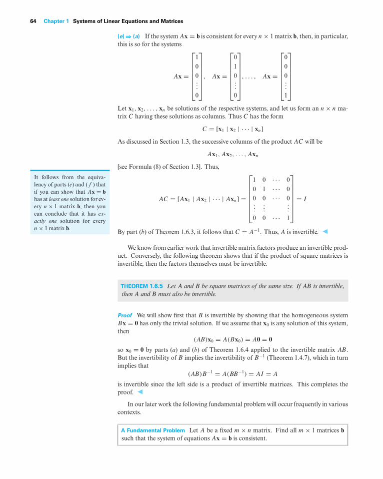
64 Chapter 1 Systems of Linear Equations and Matrices
(e) ⇒ (a) If the system Ax = b is consistent for every n × 1 matrix b, then, in particular,this is so for the systems
Ax =
⎡⎢⎢⎢⎢⎢⎢⎣
1
0
0...
0
⎤⎥⎥⎥⎥⎥⎥⎦, Ax =
⎡⎢⎢⎢⎢⎢⎢⎣
0
1
0...
0
⎤⎥⎥⎥⎥⎥⎥⎦, . . . , Ax =
⎡⎢⎢⎢⎢⎢⎢⎣
0
0
0...
1
⎤⎥⎥⎥⎥⎥⎥⎦
Let x1, x2, . . . , xn be solutions of the respective systems, and let us form an n × n ma-trix C having these solutions as columns. Thus C has the form
C = [x1 | x2 | · · · | xn]As discussed in Section 1.3, the successive columns of the product AC will be
Ax1, Ax2, . . . , Axn
[see Formula (8) of Section 1.3]. Thus,
AC = [Ax1 | Ax2 | · · · | Axn] =
⎡⎢⎢⎢⎢⎢⎢⎣
1 0 · · · 0
0 1 · · · 0
0 0 · · · 0...
......
0 0 · · · 1
⎤⎥⎥⎥⎥⎥⎥⎦ = I
By part (b) of Theorem 1.6.3, it follows that C = A−1. Thus, A is invertible.
It follows from the equiva-lency of parts (e) and ( f ) thatif you can show that Ax = bhas at least one solution for ev-ery n × 1 matrix b, then youcan conclude that it has ex-actly one solution for everyn × 1 matrix b.
We know from earlier work that invertible matrix factors produce an invertible prod-uct. Conversely, the following theorem shows that if the product of square matrices isinvertible, then the factors themselves must be invertible.
THEOREM 1.6.5 Let A and B be square matrices of the same size. If AB is invertible,then A and B must also be invertible.
Proof We will show first that B is invertible by showing that the homogeneous systemBx = 0 has only the trivial solution. If we assume that x0 is any solution of this system,then
(AB)x0 = A(Bx0) = A0 = 0
so x0 = 0 by parts (a) and (b) of Theorem 1.6.4 applied to the invertible matrix AB.But the invertibility of B implies the invertibility of B−1 (Theorem 1.4.7), which in turnimplies that
(AB)B−1 = A(BB−1) = AI = A
is invertible since the left side is a product of invertible matrices. This completes theproof.
In our later work the following fundamental problem will occur frequently in variouscontexts.
A Fundamental Problem Let A be a fixed m × n matrix. Find all m × 1 matrices bsuch that the system of equations Ax = b is consistent.
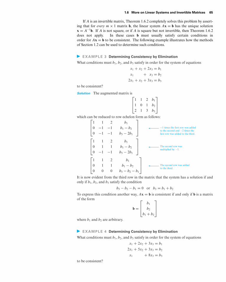
1.6 More on Linear Systems and Invertible Matrices 65
If A is an invertible matrix, Theorem 1.6.2 completely solves this problem by assert-ing that for every m × 1 matrix b, the linear system Ax = b has the unique solutionx = A−1b. If A is not square, or if A is square but not invertible, then Theorem 1.6.2does not apply. In these cases b must usually satisfy certain conditions inorder for Ax = b to be consistent. The following example illustrates how the methodsof Section 1.2 can be used to determine such conditions.
EXAMPLE 3 Determining Consistency by Elimination
What conditions must b1, b2, and b3 satisfy in order for the system of equations
x1 + x2 + 2x3 = b1
x1 + x3 = b2
2x1 + x2 + 3x3 = b3
to be consistent?
Solution The augmented matrix is⎡⎢⎣1 1 2 b1
1 0 1 b2
2 1 3 b3
⎤⎥⎦
which can be reduced to row echelon form as follows:⎡⎢⎣1 1 2 b1
0 −1 −1 b1 − b2
0 −1 −1 b3 − 2b1
⎤⎥⎦ −1 times the first row was added
to the second and −2 times thefirst row was added to the third.⎡
⎢⎣1 1 2 b1
0 1 1 b1 − b2
0 −1 −1 b3 − 2b1
⎤⎥⎦ The second row was
multiplied by −1.
⎡⎢⎣1 1 2 b1
0 1 1 b1 − b2
0 0 0 b3 − b2 − b1
⎤⎥⎦ The second row was added
to the third.
It is now evident from the third row in the matrix that the system has a solution if andonly if b1, b2, and b3 satisfy the condition
b3 − b2 − b1 = 0 or b3 = b1 + b2
To express this condition another way, Ax = b is consistent if and only if b is a matrixof the form
b =⎡⎢⎣ b1
b2
b1 + b2
⎤⎥⎦
where b1 and b2 are arbitrary.
EXAMPLE 4 Determining Consistency by Elimination
What conditions must b1, b2, and b3 satisfy in order for the system of equations
x1 + 2x2 + 3x3 = b1
2x1 + 5x2 + 3x3 = b2
x1 + 8x3 = b3
to be consistent?
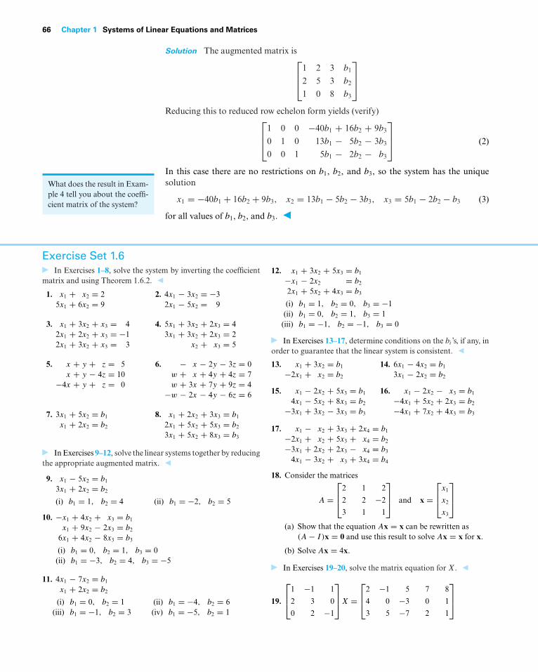
66 Chapter 1 Systems of Linear Equations and Matrices
Solution The augmented matrix is⎡⎢⎣1 2 3 b1
2 5 3 b2
1 0 8 b3
⎤⎥⎦
Reducing this to reduced row echelon form yields (verify)⎡⎢⎣1 0 0 −40b1 + 16b2 + 9b3
0 1 0 13b1 − 5b2 − 3b3
0 0 1 5b1 − 2b2 − b3
⎤⎥⎦ (2)
In this case there are no restrictions on b1, b2, and b3, so the system has the uniqueWhat does the result in Exam-ple 4 tell you about the coeffi-cient matrix of the system?
solution
x1 = −40b1 + 16b2 + 9b3, x2 = 13b1 − 5b2 − 3b3, x3 = 5b1 − 2b2 − b3 (3)
for all values of b1, b2, and b3.
Exercise Set 1.6In Exercises 1–8, solve the system by inverting the coefficient
matrix and using Theorem 1.6.2.
1. x1 + x2 = 25x1 + 6x2 = 9
2. 4x1 − 3x2 = −32x1 − 5x2 = 9
3. x1 + 3x2 + x3 = 42x1 + 2x2 + x3 = −12x1 + 3x2 + x3 = 3
4. 5x1 + 3x2 + 2x3 = 43x1 + 3x2 + 2x3 = 2
x2 + x3 = 5
5. x + y + z = 5x + y − 4z = 10
−4x + y + z = 0
6. − x − 2y − 3z = 0w + x + 4y + 4z = 7w + 3x + 7y + 9z = 4
−w − 2x − 4y − 6z = 6
7. 3x1 + 5x2 = b1
x1 + 2x2 = b2
8. x1 + 2x2 + 3x3 = b1
2x1 + 5x2 + 5x3 = b2
3x1 + 5x2 + 8x3 = b3
In Exercises 9–12, solve the linear systems together by reducingthe appropriate augmented matrix.
9. x1 − 5x2 = b1
3x1 + 2x2 = b2
(i) b1 = 1, b2 = 4 (ii) b1 = −2, b2 = 5
10. −x1 + 4x2 + x3 = b1
x1 + 9x2 − 2x3 = b2
6x1 + 4x2 − 8x3 = b3
(i) b1 = 0, b2 = 1, b3 = 0(ii) b1 = −3, b2 = 4, b3 = −5
11. 4x1 − 7x2 = b1
x1 + 2x2 = b2
(i) b1 = 0, b2 = 1 (ii) b1 = −4, b2 = 6(iii) b1 = −1, b2 = 3 (iv) b1 = −5, b2 = 1
12. x1 + 3x2 + 5x3 = b1
−x1 − 2x2 = b2
2x1 + 5x2 + 4x3 = b3
(i) b1 = 1, b2 = 0, b3 = −1(ii) b1 = 0, b2 = 1, b3 = 1
(iii) b1 = −1, b2 = −1, b3 = 0
In Exercises 13–17, determine conditions on the bi ’s, if any, inorder to guarantee that the linear system is consistent.
13. x1 + 3x2 = b1
−2x1 + x2 = b2
14. 6x1 − 4x2 = b1
3x1 − 2x2 = b2
15. x1 − 2x2 + 5x3 = b1
4x1 − 5x2 + 8x3 = b2
−3x1 + 3x2 − 3x3 = b3
16. x1 − 2x2 − x3 = b1
−4x1 + 5x2 + 2x3 = b2
−4x1 + 7x2 + 4x3 = b3
17. x1 − x2 + 3x3 + 2x4 = b1
−2x1 + x2 + 5x3 + x4 = b2
−3x1 + 2x2 + 2x3 − x4 = b3
4x1 − 3x2 + x3 + 3x4 = b4
18. Consider the matrices
A =⎡⎢⎣2 1 2
2 2 −2
3 1 1
⎤⎥⎦ and x =
⎡⎢⎣x1
x2
x3
⎤⎥⎦
(a) Show that the equation Ax = x can be rewritten as(A − I )x = 0 and use this result to solve Ax = x for x.
(b) Solve Ax = 4x.
In Exercises 19–20, solve the matrix equation for X.
19.
⎡⎢⎣1 −1 1
2 3 0
0 2 −1
⎤⎥⎦X =
⎡⎢⎣2 −1 5 7 8
4 0 −3 0 1
3 5 −7 2 1
⎤⎥⎦
1.7 Diagonal,Triangular, and Symmetric Matrices 67
20.
⎡⎢⎣−2 0 1
0 −1 −1
1 1 −4
⎤⎥⎦X =
⎡⎢⎣4 3 2 1
6 7 8 9
1 3 7 9
⎤⎥⎦
Working with Proofs
21. Let Ax = 0 be a homogeneous system of n linear equations inn unknowns that has only the trivial solution. Prove that if k
is any positive integer, then the system Akx = 0 also has onlythe trivial solution.
22. Let Ax = 0 be a homogeneous system of n linear equationsin n unknowns, and let Q be an invertible n × n matrix.Prove that Ax = 0 has only the trivial solution if and onlyif (QA)x = 0 has only the trivial solution.
23. Let Ax = b be any consistent system of linear equations, andlet x1 be a fixed solution. Prove that every solution to thesystem can be written in the form x = x1 + x0, where x0 is asolution to Ax = 0. Prove also that every matrix of this formis a solution.
24. Use part (a) of Theorem 1.6.3 to prove part (b).
True-False Exercises
TF. In parts (a)–(g) determine whether the statement is true orfalse, and justify your answer.
(a) It is impossible for a system of linear equations to have exactlytwo solutions.
(b) If A is a square matrix, and if the linear system Ax = b has aunique solution, then the linear system Ax = c also must havea unique solution.
(c) If A and B are n × n matrices such that AB = In, thenBA = In.
(d) If A and B are row equivalent matrices, then the linear systemsAx = 0 and Bx = 0 have the same solution set.
(e) Let A be an n × n matrix and S is an n × n invertible matrix.If x is a solution to the linear system (S−1AS)x = b, then Sxis a solution to the linear system Ay = Sb.
(f ) Let A be an n × n matrix. The linear system Ax = 4x has aunique solution if and only if A − 4I is an invertible matrix.
(g) Let A and B be n × n matrices. If A or B (or both) are notinvertible, then neither is AB.
Working withTechnology
T1. Colors in print media, on computer monitors, and on televi-sion screens are implemented using what are called “color mod-els”. For example, in the RGB model, colors are created by mixingpercentages of red (R), green (G), and blue (B), and in the YIQmodel (used in TV broadcasting), colors are created by mixingpercentages of luminescence (Y) with percentages of a chromi-nance factor (I) and a chrominance factor (Q). The conversionfrom the RGB model to the YIQ model is accomplished by thematrix equation⎡
⎢⎣Y
I
Q
⎤⎥⎦ =
⎡⎢⎣
.299 .587 .114
.596 −.275 −.321
.212 −.523 .311
⎤⎥⎦⎡⎢⎣
R
G
B
⎤⎥⎦
What matrix would you use to convert the YIQ model to the RGBmodel?
T2. Let
A =⎡⎢⎣
1 −2 2
4 5 1
0 3 −1
⎤⎥⎦ , B1 =
⎡⎢⎣
0
1
7
⎤⎥⎦ , B2 =
⎡⎢⎣
11
5
3
⎤⎥⎦ , B3 =
⎡⎢⎣
1
−4
2
⎤⎥⎦
Solve the linear systems Ax = B1, Ax = B2, Ax = B3 using themethod of Example 2.
1.7 Diagonal,Triangular, and Symmetric MatricesIn this section we will discuss matrices that have various special forms. These matrices arisein a wide variety of applications and will play an important role in our subsequent work.
Diagonal Matrices A square matrix in which all the entries off the main diagonal are zero is called a diagonalmatrix. Here are some examples:
[2 0
0 −5
],
⎡⎢⎣1 0 0
0 1 0
0 0 1
⎤⎥⎦,
⎡⎢⎢⎢⎣
6 0 0 0
0 −4 0 0
0 0 0 0
0 0 0 8
⎤⎥⎥⎥⎦,
[0 0
0 0
]
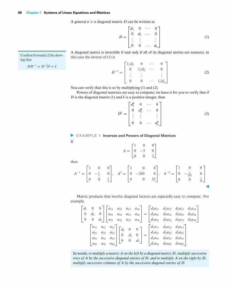
68 Chapter 1 Systems of Linear Equations and Matrices
A general n × n diagonal matrix D can be written as
D =
⎡⎢⎢⎢⎣
d1 0 · · · 00 d2 · · · 0...
......
0 0 · · · dn
⎤⎥⎥⎥⎦ (1)
A diagonal matrix is invertible if and only if all of its diagonal entries are nonzero; inConfirm Formula (2) by show-ing that
DD−1 = D−1D = I
this case the inverse of (1) is
D−1 =
⎡⎢⎢⎢⎣
1/d1 0 · · · 00 1/d2 · · · 0...
......
0 0 · · · 1/dn
⎤⎥⎥⎥⎦ (2)
You can verify that this is so by multiplying (1) and (2).Powers of diagonal matrices are easy to compute; we leave it for you to verify that if
D is the diagonal matrix (1) and k is a positive integer, then
Dk =
⎡⎢⎢⎢⎢⎣
dk1 0 · · · 0
0 dk2 · · · 0
......
...
0 0 · · · dkn
⎤⎥⎥⎥⎥⎦ (3)
EXAMPLE 1 Inverses and Powers of Diagonal Matrices
If
A =⎡⎣1 0 0
0 −3 00 0 2
⎤⎦
then
A−1 =⎡⎢⎣1 0 0
0 − 13 0
0 0 12
⎤⎥⎦, A5 =
⎡⎢⎣1 0 0
0 −243 0
0 0 32
⎤⎥⎦, A−5 =
⎡⎢⎣1 0 0
0 − 1243 0
0 0 132
⎤⎥⎦
Matrix products that involve diagonal factors are especially easy to compute. Forexample,⎡
⎢⎣d1 0 0
0 d2 0
0 0 d3
⎤⎥⎦⎡⎢⎣a11 a12 a13 a14
a21 a22 a23 a24
a31 a32 a33 a34
⎤⎥⎦ =
⎡⎢⎣d1a11 d1a12 d1a13 d1a14
d2a21 d2a22 d2a23 d2a24
d3a31 d3a32 d3a33 d3a34
⎤⎥⎦
⎡⎢⎢⎢⎣
a11 a12 a13
a21 a22 a23
a31 a32 a33
a41 a42 a43
⎤⎥⎥⎥⎦⎡⎢⎣d1 0 0
0 d2 0
0 0 d3
⎤⎥⎦ =
⎡⎢⎢⎢⎣
d1a11 d2a12 d3a13
d1a21 d2a22 d3a23
d1a31 d2a32 d3a33
d1a41 d2a42 d3a43
⎤⎥⎥⎥⎦
In words, to multiply a matrixA on the left by a diagonal matrixD,multiply successiverows of A by the successive diagonal entries ofD, and to multiply A on the right byD,
multiply successive columns of A by the successive diagonal entries of D.
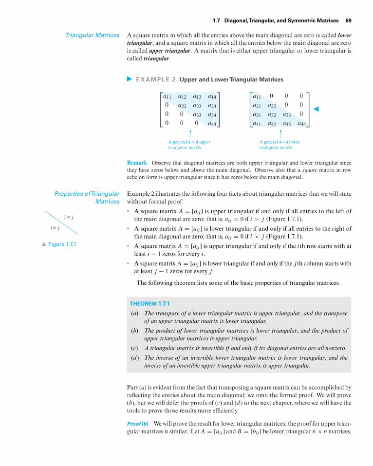
1.7 Diagonal,Triangular, and Symmetric Matrices 69
Triangular Matrices A square matrix in which all the entries above the main diagonal are zero is called lowertriangular, and a square matrix in which all the entries below the main diagonal are zerois called upper triangular. A matrix that is either upper triangular or lower triangular iscalled triangular.
EXAMPLE 2 Upper and LowerTriangular Matrices
⎡⎢⎢⎢⎣a11 a12 a13 a14
0 a22 a23 a24
0 0 a33 a34
0 0 0 a44
⎤⎥⎥⎥⎦
⎡⎢⎢⎢⎣a11 0 0 0a21 a22 0 0a31 a32 a33 0a41 a42 a43 a44
⎤⎥⎥⎥⎦
A general 4 4 uppertriangular matrix
A general 4 4 lowertriangular matrix
× ×
Remark Observe that diagonal matrices are both upper triangular and lower triangular sincethey have zeros below and above the main diagonal. Observe also that a square matrix in rowechelon form is upper triangular since it has zeros below the main diagonal.
Properties ofTriangularMatrices
Example 2 illustrates the following four facts about triangular matrices that we will statewithout formal proof:
• A square matrix A = [aij ] is upper triangular if and only if all entries to the left of
i > j
i < j
Figure 1.7.1
the main diagonal are zero; that is, aij = 0 if i > j (Figure 1.7.1).
• A square matrix A = [aij ] is lower triangular if and only if all entries to the right ofthe main diagonal are zero; that is, aij = 0 if i < j (Figure 1.7.1).
• A square matrix A = [aij ] is upper triangular if and only if the ith row starts with atleast i − 1 zeros for every i.
• A square matrix A = [aij ] is lower triangular if and only if the j th column starts withat least j − 1 zeros for every j.
The following theorem lists some of the basic properties of triangular matrices.
THEOREM 1.7.1
(a) The transpose of a lower triangular matrix is upper triangular, and the transposeof an upper triangular matrix is lower triangular.
(b) The product of lower triangular matrices is lower triangular, and the product ofupper triangular matrices is upper triangular.
(c) A triangular matrix is invertible if and only if its diagonal entries are all nonzero.
(d ) The inverse of an invertible lower triangular matrix is lower triangular, and theinverse of an invertible upper triangular matrix is upper triangular.
Part (a) is evident from the fact that transposing a square matrix can be accomplished byreflecting the entries about the main diagonal; we omit the formal proof. We will prove(b), but we will defer the proofs of (c) and (d ) to the next chapter, where we will have thetools to prove those results more efficiently.
Proof (b) We will prove the result for lower triangular matrices; the proof for upper trian-gular matrices is similar. Let A = [aij ] and B = [bij ] be lower triangular n × n matrices,
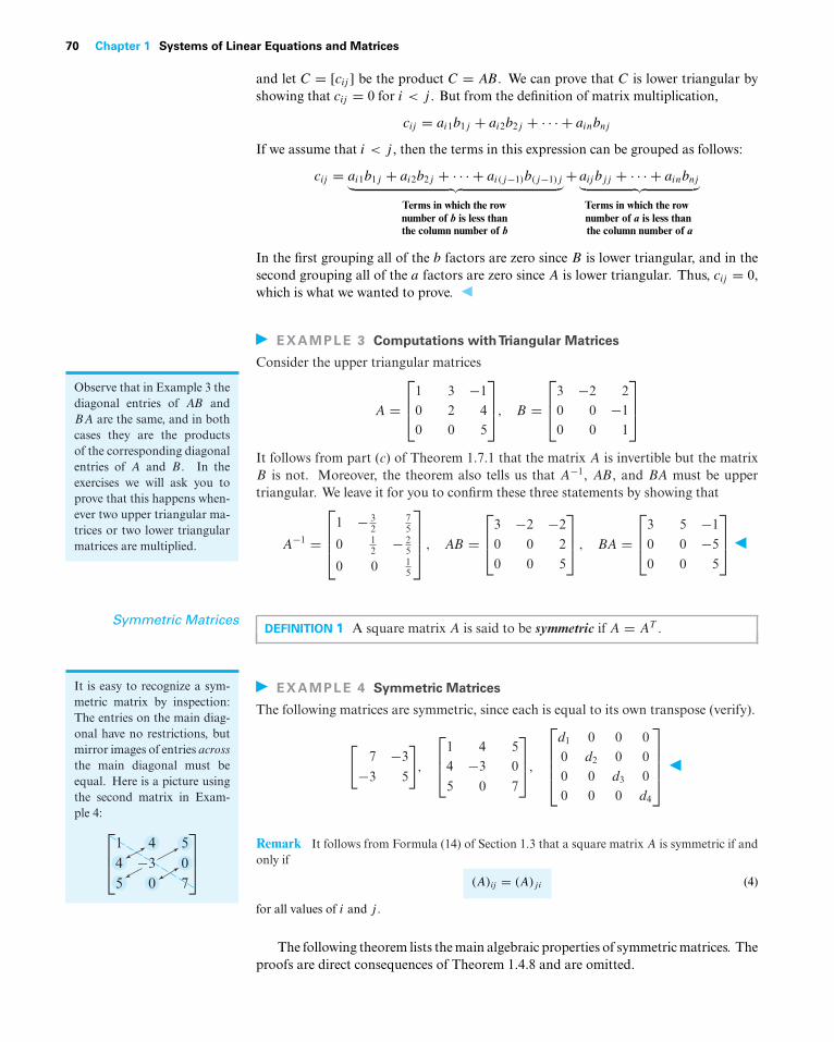
70 Chapter 1 Systems of Linear Equations and Matrices
and let C = [cij ] be the product C = AB. We can prove that C is lower triangular byshowing that cij = 0 for i < j . But from the definition of matrix multiplication,
cij = ai1b1j + ai2b2j + · · · + ainbnj
If we assume that i < j , then the terms in this expression can be grouped as follows:
cij = ai1b1j + ai2b2j + · · · + ai(j−1)b(j−1)j︸ ︷︷ ︸Terms in which the rownumber of b is less thanthe column number of b
+ aij bjj + · · · + ainbnj︸ ︷︷ ︸Terms in which the rownumber of a is less thanthe column number of a
In the first grouping all of the b factors are zero since B is lower triangular, and in thesecond grouping all of the a factors are zero since A is lower triangular. Thus, cij = 0,which is what we wanted to prove.
EXAMPLE 3 Computations withTriangular Matrices
Consider the upper triangular matrices
A =⎡⎢⎣1 3 −1
0 2 40 0 5
⎤⎥⎦, B =
⎡⎢⎣3 −2 2
0 0 −10 0 1
⎤⎥⎦
It follows from part (c) of Theorem 1.7.1 that the matrix A is invertible but the matrixB is not. Moreover, the theorem also tells us that A−1, AB, and BA must be uppertriangular. We leave it for you to confirm these three statements by showing that
Observe that in Example 3 thediagonal entries of AB andBA are the same, and in bothcases they are the productsof the corresponding diagonalentries of A and B. In theexercises we will ask you toprove that this happens when-ever two upper triangular ma-trices or two lower triangularmatrices are multiplied. A−1 =
⎡⎢⎢⎣
1 − 32
75
0 12 − 2
5
0 0 15
⎤⎥⎥⎦ , AB =
⎡⎢⎣3 −2 −2
0 0 2
0 0 5
⎤⎥⎦ , BA =
⎡⎢⎣3 5 −1
0 0 −5
0 0 5
⎤⎥⎦
Symmetric MatricesDEFINITION 1 A square matrix A is said to be symmetric if A = AT .
EXAMPLE 4 Symmetric Matrices
The following matrices are symmetric, since each is equal to its own transpose (verify).
It is easy to recognize a sym-metric matrix by inspection:The entries on the main diag-onal have no restrictions, butmirror images of entries acrossthe main diagonal must beequal. Here is a picture usingthe second matrix in Exam-ple 4:
⎡⎢⎣
1 4 54 3 05 0 7
⎤⎥⎦
[7 −3
−3 5
],
⎡⎢⎣1 4 5
4 −3 0
5 0 7
⎤⎥⎦,
⎡⎢⎢⎢⎣
d1 0 0 00 d2 0 00 0 d3 00 0 0 d4
⎤⎥⎥⎥⎦
Remark It follows from Formula (14) of Section 1.3 that a square matrix A is symmetric if andonly if
(A)ij = (A)ji (4)
for all values of i and j .
The following theorem lists the main algebraic properties of symmetric matrices. Theproofs are direct consequences of Theorem 1.4.8 and are omitted.
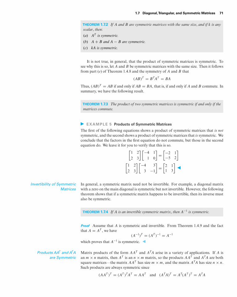
1.7 Diagonal,Triangular, and Symmetric Matrices 71
THEOREM 1.7.2 If A and B are symmetric matrices with the same size, and if k is anyscalar, then:
(a) AT is symmetric.
(b) A + B and A − B are symmetric.
(c) kA is symmetric.
It is not true, in general, that the product of symmetric matrices is symmetric. Tosee why this is so, let A and B be symmetric matrices with the same size. Then it followsfrom part (e) of Theorem 1.4.8 and the symmetry of A and B that
(AB)T = BTAT = BA
Thus, (AB)T = AB if and only if AB = BA, that is, if and only if A and B commute. Insummary, we have the following result.
THEOREM 1.7.3 The product of two symmetric matrices is symmetric if and only if thematrices commute.
EXAMPLE 5 Products of Symmetric Matrices
The first of the following equations shows a product of symmetric matrices that is notsymmetric, and the second shows a product of symmetric matrices that is symmetric. Weconclude that the factors in the first equation do not commute, but those in the secondequation do. We leave it for you to verify that this is so.[
1 2
2 3
] [−4 1
1 0
]=[−2 1−5 2
][
1 2
2 3
] [−4 3
3 −1
]=[
2 11 3
]
Invertibility of SymmetricMatrices
In general, a symmetric matrix need not be invertible. For example, a diagonal matrixwith a zero on the main diagonal is symmetric but not invertible. However, the followingtheorem shows that if a symmetric matrix happens to be invertible, then its inverse mustalso be symmetric.
THEOREM 1.7.4 If A is an invertible symmetric matrix, then A−1 is symmetric.
Proof Assume that A is symmetric and invertible. From Theorem 1.4.9 and the factthat A = AT , we have
(A−1)T = (AT )−1 = A−1
which proves that A−1 is symmetric.
Products AAT and ATAare Symmetric
Matrix products of the form AAT and ATA arise in a variety of applications. If A isan m × n matrix, then AT is an n × m matrix, so the products AAT and ATA are bothsquare matrices—the matrix AAT has size m × m, and the matrix ATA has size n × n.Such products are always symmetric since
(AAT )T = (AT )TAT = AAT and (ATA)T = AT(AT )T = ATA
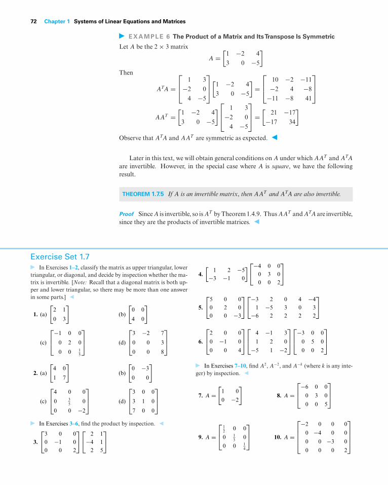
72 Chapter 1 Systems of Linear Equations and Matrices
EXAMPLE 6 The Product of a Matrix and ItsTranspose Is Symmetric
Let A be the 2 × 3 matrix
A =[
1 −2 4
3 0 −5
]Then
ATA =⎡⎢⎣ 1 3
−2 0
4 −5
⎤⎥⎦[1 −2 4
3 0 −5
]=⎡⎢⎣ 10 −2 −11
−2 4 −8
−11 −8 41
⎤⎥⎦
AAT =[
1 −2 4
3 0 −5
]⎡⎢⎣ 1 3
−2 0
4 −5
⎤⎥⎦ =
[21 −17
−17 34
]
Observe that ATA and AAT are symmetric as expected.
Later in this text, we will obtain general conditions on A under which AAT and ATA
are invertible. However, in the special case where A is square, we have the followingresult.
THEOREM 1.7.5 If A is an invertible matrix, then AAT and ATA are also invertible.
Proof SinceA is invertible, so isAT by Theorem 1.4.9. ThusAAT andATAare invertible,since they are the products of invertible matrices.
Exercise Set 1.7In Exercises 1–2, classify the matrix as upper triangular, lower
triangular, or diagonal, and decide by inspection whether the ma-trix is invertible. [Note: Recall that a diagonal matrix is both up-per and lower triangular, so there may be more than one answerin some parts.]
1. (a)
[2 1
0 3
](b)
[0 0
4 0
]
(c)
⎡⎢⎣−1 0 0
0 2 0
0 0 15
⎤⎥⎦ (d)
⎡⎢⎣
3 −2 7
0 0 3
0 0 8
⎤⎥⎦
2. (a)
[4 0
1 7
](b)
[0 −3
0 0
]
(c)
⎡⎢⎣
4 0 0
0 35 0
0 0 −2
⎤⎥⎦ (d)
⎡⎢⎣
3 0 0
3 1 0
7 0 0
⎤⎥⎦
In Exercises 3–6, find the product by inspection.
3.
⎡⎣3 0 0
0 −1 00 0 2
⎤⎦⎡⎣ 2 1−4 1
2 5
⎤⎦
4.[
1 2 −5−3 −1 0
]⎡⎣−4 0 00 3 00 0 2
⎤⎦
5.
⎡⎣5 0 0
0 2 00 0 −3
⎤⎦⎡⎣−3 2 0 4 −4
1 −5 3 0 3−6 2 2 2 2
⎤⎦
6.
⎡⎢⎣2 0 0
0 −1 0
0 0 4
⎤⎥⎦⎡⎢⎣ 4 −1 3
1 2 0
−5 1 −2
⎤⎥⎦⎡⎢⎣−3 0 0
0 5 0
0 0 2
⎤⎥⎦
In Exercises 7–10, find A2, A−2, and A−k (where k is any inte-ger) by inspection.
7. A =[
1 0
0 −2
]8. A =
⎡⎢⎣−6 0 0
0 3 0
0 0 5
⎤⎥⎦
9. A =⎡⎢⎣
12 0 0
0 13 0
0 0 14
⎤⎥⎦ 10. A =
⎡⎢⎢⎢⎣−2 0 0 0
0 −4 0 0
0 0 −3 0
0 0 0 2
⎤⎥⎥⎥⎦
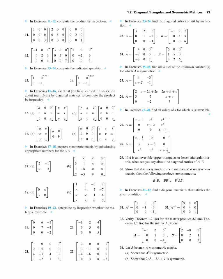
1.7 Diagonal,Triangular, and Symmetric Matrices 73
In Exercises 11–12, compute the product by inspection.
11.
⎡⎢⎣
1 0 0
0 0 0
0 0 3
⎤⎥⎦⎡⎢⎣
2 0 0
0 5 0
0 0 0
⎤⎥⎦⎡⎢⎣
0 0 0
0 2 0
0 0 1
⎤⎥⎦
12.
⎡⎢⎣−1 0 0
0 2 0
0 0 4
⎤⎥⎦⎡⎢⎣
3 0 0
0 5 0
0 0 7
⎤⎥⎦⎡⎢⎣
5 0 0
0 −2 0
0 0 3
⎤⎥⎦
In Exercises 13–14, compute the indicated quantity.
13.
[1 0
0 −1
]39
14.
[1 0
0 −1
]1000
In Exercises 15–16, use what you have learned in this sectionabout multiplying by diagonal matrices to compute the productby inspection.
15. (a)
⎡⎢⎣
a 0 0
0 b 0
0 0 c
⎤⎥⎦⎡⎢⎣
u v
w x
y z
⎤⎥⎦ (b)
⎡⎢⎣
r s t
u v w
x y z
⎤⎥⎦⎡⎢⎣
a 0 0
0 b 0
0 0 c
⎤⎥⎦
16. (a)
⎡⎢⎣
u v
w x
y z
⎤⎥⎦[a 0
0 b
](b)
⎡⎢⎣
a 0 0
0 b 0
0 0 c
⎤⎥⎦⎡⎢⎣
r s t
u v w
x y z
⎤⎥⎦
In Exercises 17–18, create a symmetric matrix by substitutingappropriate numbers for the ×’s.
17. (a)
[2 −1
× 3
](b)
⎡⎢⎢⎢⎣
1 × × ×3 1 × ×7 −8 0 ×2 −3 9 0
⎤⎥⎥⎥⎦
18. (a)
[0 ×3 0
](b)
⎡⎢⎢⎢⎣
1 7 −3 2
× 4 5 −7
× × 1 −6
× × × 3
⎤⎥⎥⎥⎦
In Exercises 19–22, determine by inspection whether the ma-trix is invertible.
19.
⎡⎢⎣0 6 −1
0 7 −4
0 0 −2
⎤⎥⎦ 20.
⎡⎢⎣−1 2 4
0 3 0
0 0 5
⎤⎥⎦
21.
⎡⎢⎢⎢⎣
1 0 0 0
2 −5 0 0
4 −3 4 0
1 −2 1 3
⎤⎥⎥⎥⎦ 22.
⎡⎢⎢⎢⎣
2 0 0 0
−3 −1 0 0
−4 −6 0 0
0 3 8 −5
⎤⎥⎥⎥⎦
In Exercises 23–24, find the diagonal entries of AB by inspec-tion.
23. A =⎡⎢⎣3 2 6
0 1 −2
0 0 −1
⎤⎥⎦ , B =
⎡⎢⎣−1 2 7
0 5 3
0 0 6
⎤⎥⎦
24. A =⎡⎢⎣ 4 0 0
−2 0 0
−3 0 7
⎤⎥⎦ , B =
⎡⎢⎣6 0 0
1 5 0
3 2 6
⎤⎥⎦
In Exercises 25–26, find all values of the unknown constant(s)for which A is symmetric.
25. A =[
4 −3
a + 5 −1
]
26. A =⎡⎢⎣2 a − 2b + 2c 2a + b + c
3 5 a + c
0 −2 7
⎤⎥⎦
In Exercises 27–28, find all values of x for which A is invertible.
27. A =⎡⎢⎣x − 1 x2 x4
0 x + 2 x3
0 0 x − 4
⎤⎥⎦
28. A =
⎡⎢⎢⎣
x − 12 0 0
x x − 13 0
x2 x3 x + 14
⎤⎥⎥⎦
29. If A is an invertible upper triangular or lower triangular ma-trix, what can you say about the diagonal entries of A−1?
30. Show that if A is a symmetric n × n matrix and B is any n × m
matrix, then the following products are symmetric:
BTB, BBT , BTAB
In Exercises 31–32, find a diagonal matrix A that satisfies thegiven condition.
31. A5 =⎡⎣1 0 0
0 −1 00 0 −1
⎤⎦ 32. A−2 =
⎡⎣9 0 0
0 4 00 0 1
⎤⎦
33. Verify Theorem 1.7.1(b) for the matrix product AB and The-orem 1.7.1(d) for the matrix A, where
A =⎡⎢⎣−1 2 5
0 1 3
0 0 −4
⎤⎥⎦, B =
⎡⎢⎣2 −8 0
0 2 1
0 0 3
⎤⎥⎦
34. Let A be an n × n symmetric matrix.
(a) Show that A2 is symmetric.
(b) Show that 2A2 − 3A + I is symmetric.
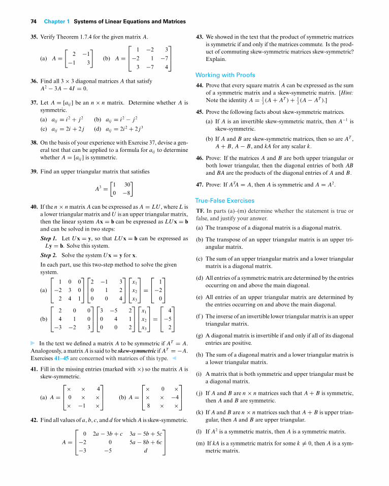
74 Chapter 1 Systems of Linear Equations and Matrices
35. Verify Theorem 1.7.4 for the given matrix A.
(a) A =[
2 −1
−1 3
](b) A =
⎡⎢⎣ 1 −2 3
−2 1 −7
3 −7 4
⎤⎥⎦
36. Find all 3 × 3 diagonal matrices A that satisfyA2 − 3A − 4I = 0.
37. Let A = [aij ] be an n × n matrix. Determine whether A issymmetric.
(a) aij = i2 + j 2 (b) aij = i2 − j 2
(c) aij = 2i + 2j (d) aij = 2i2 + 2j 3
38. On the basis of your experience with Exercise 37, devise a gen-eral test that can be applied to a formula for aij to determinewhether A = [aij ] is symmetric.
39. Find an upper triangular matrix that satisfies
A3 =[
1 30
0 −8
]
40. If the n × n matrix A can be expressed as A = LU , where L isa lower triangular matrix and U is an upper triangular matrix,then the linear system Ax = b can be expressed as LUx = band can be solved in two steps:
Step 1. Let Ux = y, so that LUx = b can be expressed asLy = b. Solve this system.
Step 2. Solve the system Ux = y for x.
In each part, use this two-step method to solve the givensystem.
(a)
⎡⎢⎣ 1 0 0
−2 3 0
2 4 1
⎤⎥⎦⎡⎢⎣2 −1 3
0 1 2
0 0 4
⎤⎥⎦⎡⎢⎣x1
x2
x3
⎤⎥⎦ =
⎡⎢⎣ 1
−2
0
⎤⎥⎦
(b)
⎡⎢⎣ 2 0 0
4 1 0
−3 −2 3
⎤⎥⎦⎡⎢⎣3 −5 2
0 4 1
0 0 2
⎤⎥⎦⎡⎢⎣x1
x2
x3
⎤⎥⎦ =
⎡⎢⎣ 4
−5
2
⎤⎥⎦
In the text we defined a matrix A to be symmetric if AT = A.Analogously, a matrix A is said to be skew-symmetric if AT = −A.Exercises 41–45 are concerned with matrices of this type.
41. Fill in the missing entries (marked with ×) so the matrix A isskew-symmetric.
(a) A =⎡⎢⎣× × 4
0 × ×× −1 ×
⎤⎥⎦ (b) A =
⎡⎢⎣× 0 ×× × −4
8 × ×
⎤⎥⎦
42. Find all values of a, b, c, and d for which A is skew-symmetric.
A =⎡⎢⎣ 0 2a − 3b + c 3a − 5b + 5c
−2 0 5a − 8b + 6c
−3 −5 d
⎤⎥⎦
43. We showed in the text that the product of symmetric matricesis symmetric if and only if the matrices commute. Is the prod-uct of commuting skew-symmetric matrices skew-symmetric?Explain.
Working with Proofs
44. Prove that every square matrix A can be expressed as the sumof a symmetric matrix and a skew-symmetric matrix. [Hint:Note the identity A = 1
2 (A + AT ) + 12 (A − AT ).]
45. Prove the following facts about skew-symmetric matrices.
(a) If A is an invertible skew-symmetric matrix, then A−1 isskew-symmetric.
(b) If A and B are skew-symmetric matrices, then so are AT ,A + B, A − B, and kA for any scalar k.
46. Prove: If the matrices A and B are both upper triangular orboth lower triangular, then the diagonal entries of both AB
and BA are the products of the diagonal entries of A and B.
47. Prove: If ATA = A, then A is symmetric and A = A2.
True-False Exercises
TF. In parts (a)–(m) determine whether the statement is true orfalse, and justify your answer.
(a) The transpose of a diagonal matrix is a diagonal matrix.
(b) The transpose of an upper triangular matrix is an upper tri-angular matrix.
(c) The sum of an upper triangular matrix and a lower triangularmatrix is a diagonal matrix.
(d) All entries of a symmetric matrix are determined by the entriesoccurring on and above the main diagonal.
(e) All entries of an upper triangular matrix are determined bythe entries occurring on and above the main diagonal.
(f ) The inverse of an invertible lower triangular matrix is an uppertriangular matrix.
(g) A diagonal matrix is invertible if and only if all of its diagonalentries are positive.
(h) The sum of a diagonal matrix and a lower triangular matrix isa lower triangular matrix.
(i) A matrix that is both symmetric and upper triangular must bea diagonal matrix.
( j) If A and B are n × n matrices such that A + B is symmetric,then A and B are symmetric.
(k) If A and B are n × n matrices such that A + B is upper trian-gular, then A and B are upper triangular.
(l) If A2 is a symmetric matrix, then A is a symmetric matrix.
(m) If kA is a symmetric matrix for some k �= 0, then A is a sym-metric matrix.
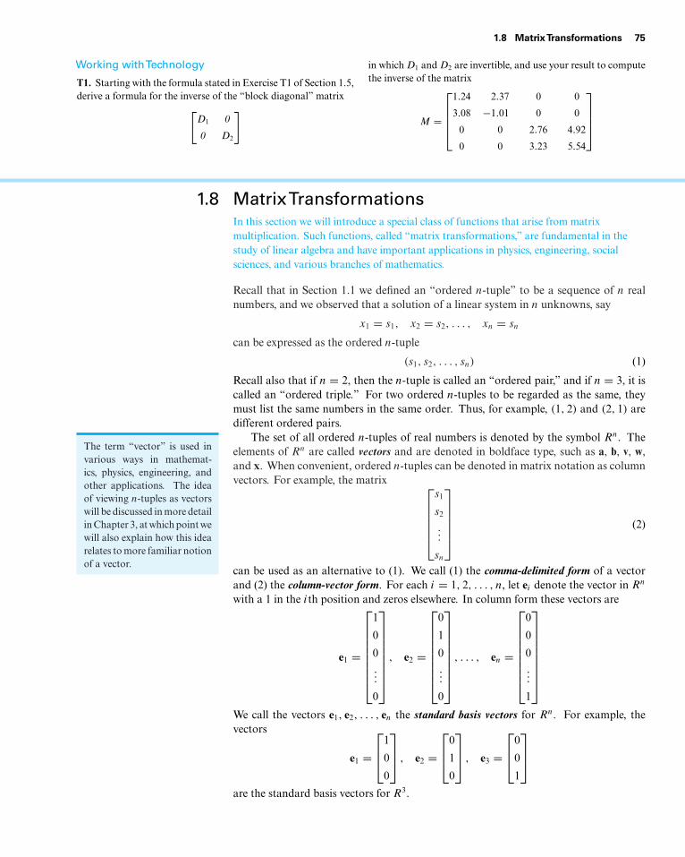
1.8 MatrixTransformations 75
Working withTechnology
T1. Starting with the formula stated in Exercise T1 of Section 1.5,derive a formula for the inverse of the “block diagonal” matrix[
D1 0
0 D2
]
in which D1 and D2 are invertible, and use your result to computethe inverse of the matrix
M =
⎡⎢⎢⎢⎣
1.24 2.37 0 0
3.08 −1.01 0 0
0 0 2.76 4.92
0 0 3.23 5.54
⎤⎥⎥⎥⎦
1.8 MatrixTransformationsIn this section we will introduce a special class of functions that arise from matrixmultiplication. Such functions, called “matrix transformations,” are fundamental in thestudy of linear algebra and have important applications in physics, engineering, socialsciences, and various branches of mathematics.
Recall that in Section 1.1 we defined an “ordered n-tuple” to be a sequence of n realnumbers, and we observed that a solution of a linear system in n unknowns, say
x1 = s1, x2 = s2, . . . , xn = sn
can be expressed as the ordered n-tuple
(s1, s2, . . . , sn) (1)
Recall also that if n = 2, then the n-tuple is called an “ordered pair,” and if n = 3, it iscalled an “ordered triple.” For two ordered n-tuples to be regarded as the same, theymust list the same numbers in the same order. Thus, for example, (1, 2) and (2, 1) aredifferent ordered pairs.
The set of all ordered n-tuples of real numbers is denoted by the symbol Rn. TheThe term “vector” is used invarious ways in mathemat-ics, physics, engineering, andother applications. The ideaof viewing n-tuples as vectorswill be discussed in more detailin Chapter 3, at which point wewill also explain how this idearelates to more familiar notionof a vector.
elements of Rn are called vectors and are denoted in boldface type, such as a, b, v, w,and x. When convenient, ordered n-tuples can be denoted in matrix notation as columnvectors. For example, the matrix ⎡
⎢⎢⎢⎢⎣s1
s2
...
sn
⎤⎥⎥⎥⎥⎦ (2)
can be used as an alternative to (1). We call (1) the comma-delimited form of a vectorand (2) the column-vector form. For each i = 1, 2, . . . , n, let ei denote the vector in Rn
with a 1 in the ith position and zeros elsewhere. In column form these vectors are
e1 =
⎡⎢⎢⎢⎢⎢⎢⎢⎣
1
0
0...
0
⎤⎥⎥⎥⎥⎥⎥⎥⎦
, e2 =
⎡⎢⎢⎢⎢⎢⎢⎢⎣
0
1
0...
0
⎤⎥⎥⎥⎥⎥⎥⎥⎦
, . . . , en =
⎡⎢⎢⎢⎢⎢⎢⎢⎣
0
0
0...
1
⎤⎥⎥⎥⎥⎥⎥⎥⎦
We call the vectors e1, e2, . . . , en the standard basis vectors for Rn. For example, thevectors
e1 =⎡⎢⎣1
0
0
⎤⎥⎦ , e2 =
⎡⎢⎣0
1
0
⎤⎥⎦ , e3 =
⎡⎢⎣0
0
1
⎤⎥⎦
are the standard basis vectors for R3.
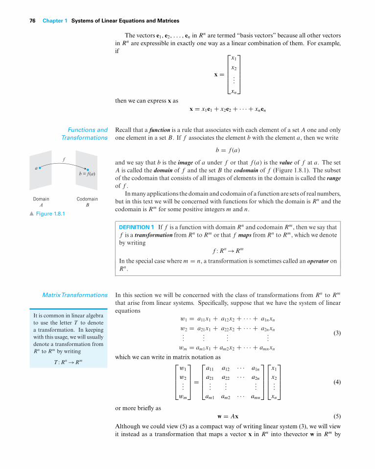
76 Chapter 1 Systems of Linear Equations and Matrices
The vectors e1, e2, . . . , en in Rn are termed “basis vectors” because all other vectorsin Rn are expressible in exactly one way as a linear combination of them. For example,if
x =
⎡⎢⎢⎢⎢⎣
x1
x2
...
xn
⎤⎥⎥⎥⎥⎦
then we can express x asx = x1e1 + x2e2 + · · · + xnen
Functions andTransformations
Recall that a function is a rule that associates with each element of a set A one and onlyone element in a set B. If f associates the element b with the element a, then we write
b = f(a)
and we say that b is the image of a under f or that f(a) is the value of f at a. The setA is called the domain of f and the set B the codomain of f (Figure 1.8.1). The subseta
b = f (a)
f
Domain
ACodomain
B
Figure 1.8.1
of the codomain that consists of all images of elements in the domain is called the rangeof f .
In many applications the domain and codomain of a function are sets of real numbers,but in this text we will be concerned with functions for which the domain is Rn and thecodomain is Rm for some positive integers m and n.
DEFINITION 1 If f is a function with domain Rn and codomain Rm, then we say thatf is a transformation from Rn to Rm or that f maps from Rn to Rm, which we denoteby writing
f : Rn →Rm
In the special case where m = n, a transformation is sometimes called an operator onRn.
MatrixTransformations In this section we will be concerned with the class of transformations from Rn to Rm
that arise from linear systems. Specifically, suppose that we have the system of linear
It is common in linear algebrato use the letter T to denotea transformation. In keepingwith this usage, we will usuallydenote a transformation fromRn to Rm by writing
T : Rn →Rm
equationsw1 = a11x1 + a12x2 + · · · + a1nxn
w2 = a21x1 + a22x2 + · · · + a2nxn...
......
...
wm = am1x1 + am2x2 + · · · + amnxn
(3)
which we can write in matrix notation as⎡⎢⎢⎢⎣
w1
w2...
wm
⎤⎥⎥⎥⎦ =
⎡⎢⎢⎢⎣
a11 a12 · · · a1n
a21 a22 · · · a2n...
......
am1 am2 · · · amn
⎤⎥⎥⎥⎦⎡⎢⎢⎢⎣
x1
x2...
xn
⎤⎥⎥⎥⎦ (4)
or more briefly asw = Ax (5)
Although we could view (5) as a compact way of writing linear system (3), we will viewit instead as a transformation that maps a vector x in Rn into thevector w in Rm by
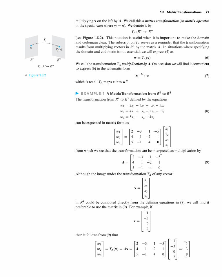
1.8 MatrixTransformations 77
multiplying x on the left by A. We call this a matrix transformation (or matrix operatorin the special case where m = n). We denote it by
TA: Rn → Rm
(see Figure 1.8.2). This notation is useful when it is important to make the domain
x
TA : Rn → Rm
TA(x)
TA
Rn Rm
Figure 1.8.2
and codomain clear. The subscript on TA serves as a reminder that the transformationresults from multiplying vectors in Rn by the matrix A. In situations where specifyingthe domain and codomain is not essential, we will express (4) as
w = TA(x) (6)
We call the transformation TA multiplication by A. On occasion we will find it convenientto express (6) in the schematic form
xTA−→ w (7)
which is read “TA maps x into w.”
EXAMPLE 1 A MatrixTransformation from R4 to R3
The transformation from R4 to R3 defined by the equations
w1 = 2x1 − 3x2 + x3 − 5x4
w2 = 4x1 + x2 − 2x3 + x4
w3 = 5x1 − x2 + 4x3
(8)
can be expressed in matrix form as⎡⎢⎣w1
w2
w3
⎤⎥⎦ =
⎡⎢⎣2 −3 1 −5
4 1 −2 1
5 −1 4 0
⎤⎥⎦⎡⎢⎢⎢⎣
x1
x2
x3
x4
⎤⎥⎥⎥⎦
from which we see that the transformation can be interpreted as multiplication by
A =⎡⎢⎣2 −3 1 −5
4 1 −2 1
5 −1 4 0
⎤⎥⎦ (9)
Although the image under the transformation TA of any vector
x =
⎡⎢⎢⎢⎣
x1
x2
x3
x4
⎤⎥⎥⎥⎦
in R4 could be computed directly from the defining equations in (8), we will find itpreferable to use the matrix in (9). For example, if
x =
⎡⎢⎢⎢⎣
1
−3
0
2
⎤⎥⎥⎥⎦
then it follows from (9) that⎡⎢⎣w1
w2
w3
⎤⎥⎦ = TA(x) = Ax =
⎡⎢⎣2 −3 1 −5
4 1 −2 1
5 −1 4 0
⎤⎥⎦⎡⎢⎢⎢⎣
1
−3
0
2
⎤⎥⎥⎥⎦ =
⎡⎢⎣1
3
8
⎤⎥⎦
78 Chapter 1 Systems of Linear Equations and Matrices
EXAMPLE 2 ZeroTransformations
If 0 is the m × n zero matrix, then
T0(x) = 0x = 0
so multiplication by zero maps every vector in Rn into the zero vector in Rm. We call T0the zero transformation from Rn to Rm.
EXAMPLE 3 Identity Operators
If I is the n × n identity matrix, then
TI (x) = Ix = x
so multiplication by I maps every vector in Rn to itself. We call TI the identity operatoron Rn.
Properties of MatrixTransformations
The following theorem lists four basic properties of matrix transformations that followfrom properties of matrix multiplication.
THEOREM 1.8.1 For every matrix A the matrix transformation TA: Rn →Rm has thefollowing properties for all vectors u and v and for every scalar k:
(a) TA(0) = 0
(b) TA(ku) = kTA(u) [Homogeneity property]
(c) TA(u + v) = TA(u) + TA(v) [Additivity property]
(d ) TA(u − v) = TA(u) − TA(v)
Proof All four parts are restatements of the following properties of matrix arithmeticgiven in Theorem 1.4.1:
A0 = 0, A(ku) = k(Au), A(u + v) = Au + Av, A(u − v) = Au − Av
It follows from parts (b) and (c) of Theorem 1.8.1 that a matrix transformation mapsa linear combination of vectors in Rn into the corresponding linear combination ofvectors in Rm in the sense that
TA(k1u1 + k2u2 + · · · + krur ) = k1TA(u1) + k2TA(u2) + · · · + krTA(ur ) (10)
Matrix transformations are not the only kinds of transformations. For example, if
w1 = x21 + x2
2
w2 = x1x2(11)
then there are no constants a, b, c, and d for which[w1
w2
]=[a b
c d
][x1
x2
]=[x2
1 + x22
x1x2
]
so that the equations in (11) do not define a matrix transformation from R2 to R2.
1.8 MatrixTransformations 79
This leads us to the following two questions.
Question 1. Are there algebraic properties of a transformation T : Rn →Rm that canbe used to determine whether T is a matrix transformation?
Question 2. If we discover that a transformation T : Rn →Rm is a matrix transfor-mation, how can we find a matrix for it?
The following theorem and its proof will provide the answers.
THEOREM 1.8.2 T : Rn →Rm is a matrix transformation if and only if the followingrelationships hold for all vectors u and v in Rn and for every scalar k:
(i) T (u + v) = T (u) + T (v) [Additivity property]
(ii) T (ku) = kT (u) [Homogeneity property]
Proof If T is a matrix transformation, then properties (i) and (ii) follow respectivelyfrom parts (c) and (b) of Theorem 1.8.1.
Conversely, assume that properties (i) and (ii) hold. We must show that there existsan m × n matrix A such that
T (x) = Ax
for every vector x in Rn. Recall that the derivation of Formula (10) used only theadditivity and homogeneity properties of TA. Since we are assuming that T has thoseproperties, it must be true that
T (k1u1 + k2u2 + · · · + krur ) = k1T (u1) + k2T (u2) + · · · + krT (ur ) (12)
for all scalars k1, k2, . . . , kr and all vectors u1, u2, . . . , ur in Rn. Let A be the matrix
A = [T (e1) | T (e2) | · · · | T (en)] (13)
where e1, e2, . . . , en are the standard basis vectors for Rn. It follows from Theorem 1.3.1that Ax is a linear combination of the columns of A in which the successive coefficientsare the entries x1, x2, . . . , xn of x. That is,
Ax = x1T (e1) + x2T (e2) + · · · + xnT (en)
Using Formula (10) we can rewrite this as
Ax = T (x1e1 + x2e2 + · · · + xnen) = T (x)
which completes the proof.
The additivity and homogeneity properties in Theorem 1.8.2 are called linearityconditions, and a transformation that satisfies these conditions is called a linear transfor-mation. Using this terminology Theorem 1.8.2 can be restated as follows.
Theorem 1.8.3 tells us thatfor transformations from Rn toRm, the terms “matrix trans-formation” and “linear trans-formation” are synonymous.
THEOREM1.8.3 Every linear transformation fromRn toRm is amatrix transformation,and conversely, every matrix transformation from Rn to Rm is a linear transformation.
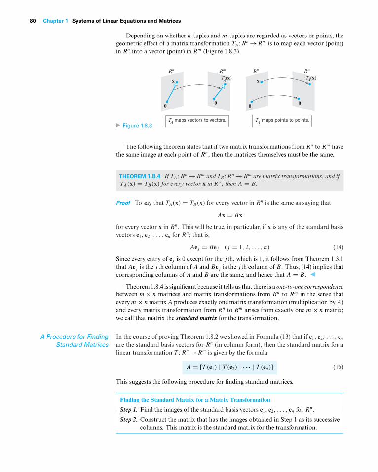
80 Chapter 1 Systems of Linear Equations and Matrices
Depending on whether n-tuples and m-tuples are regarded as vectors or points, thegeometric effect of a matrix transformation TA: Rn →Rm is to map each vector (point)in Rn into a vector (point) in Rm (Figure 1.8.3).
Figure 1.8.3
xTA(x)
Rn Rm
0 0
TA maps points to points.
xTA(x)
Rn Rm
00
TA maps vectors to vectors.
The following theorem states that if two matrix transformations from Rn to Rm havethe same image at each point of Rn, then the matrices themselves must be the same.
THEOREM 1.8.4 If TA: Rn →Rm and TB : Rn →Rm are matrix transformations, and ifTA(x) = TB(x) for every vector x in Rn, then A = B.
Proof To say that TA(x) = TB(x) for every vector in Rn is the same as saying that
Ax = Bx
for every vector x in Rn. This will be true, in particular, if x is any of the standard basisvectors e1, e2, . . . , en for Rn; that is,
Aej = Bej (j = 1, 2, . . . , n) (14)
Since every entry of ej is 0 except for the j th, which is 1, it follows from Theorem 1.3.1that Aej is the j th column of A and Bej is the j th column of B. Thus, (14) implies thatcorresponding columns of A and B are the same, and hence that A = B.
Theorem 1.8.4 is significant because it tells us that there is aone-to-one correspondencebetween m × n matrices and matrix transformations from Rn to Rm in the sense thatevery m × n matrix A produces exactly one matrix transformation (multiplication by A)and every matrix transformation from Rn to Rm arises from exactly one m × n matrix;we call that matrix the standard matrix for the transformation.
A Procedure for FindingStandard Matrices
In the course of proving Theorem 1.8.2 we showed in Formula (13) that if e1, e2, . . . , en
are the standard basis vectors for Rn (in column form), then the standard matrix for alinear transformation T : Rn →Rm is given by the formula
A = [T (e1) | T (e2) | · · · | T (en)] (15)
This suggests the following procedure for finding standard matrices.
Finding the Standard Matrix for a Matrix Transformation
Step 1. Find the images of the standard basis vectors e1, e2, . . . , en for Rn.
Step 2. Construct the matrix that has the images obtained in Step 1 as its successivecolumns. This matrix is the standard matrix for the transformation.
1.8 MatrixTransformations 81
EXAMPLE 4 Finding a Standard Matrix
Find the standard matrix A for the linear transformation T : R2 →R2 defined by theformula
T
([x1
x2
])=⎡⎢⎣ 2x1 + x2
x1 − 3x2
−x1 + x2
⎤⎥⎦ (16)
Solution We leave it for you to verify that
T (e1) = T
([1
0
])=⎡⎢⎣ 2
1
−1
⎤⎥⎦ and T (e2) = T
([0
1
])=⎡⎢⎣ 1
−3
1
⎤⎥⎦
Thus, it follows from Formulas (15) and (16) that the standard matrix is
A = [T (e1) | T (e2)] =⎡⎢⎣ 2 1
1 −3
−1 1
⎤⎥⎦
EXAMPLE 5 Computing with Standard Matrices
For the linear transformation in Example 4, use the standard matrix A obtained in thatexample to find
T
([1
4
])
Solution The transformation is multiplication by A, soAlthough we could have ob-tained the result in Example 5by substituting values for thevariables in (13), the methodused in Example 5 is preferablefor large-scale problems in thatmatrix multiplication is bettersuited for computer computa-tions.
T
([1
4
])=⎡⎢⎣ 2 1
1 −3
−1 1
⎤⎥⎦[
1
4
]=⎡⎢⎣ 6
−11
3
⎤⎥⎦
For transformation problems posed in comma-delimited form, a good procedure isto rewrite the problem in column-vector form and use the methods previously illustrated.
EXAMPLE 6 Finding a Standard Matrix
Rewrite the transformation T (x1, x2) = (3x1 + x2, 2x1 − 4x2) in column-vector formand find its standard matrix.
Solution
T
([x1
x2
])=[
3x1 + x2
2x1 − 4x2
]=[
3 1
2 −2
][x1
x2
]Thus, the standard matrix is [
3 1
2 −2
]
Remark This section is but a first step in the study of linear transformations, which is one of themajor themes in this text. We will delve deeper into this topic in Chapter 4, at which point we willhave more background and a richer source of examples to work with.
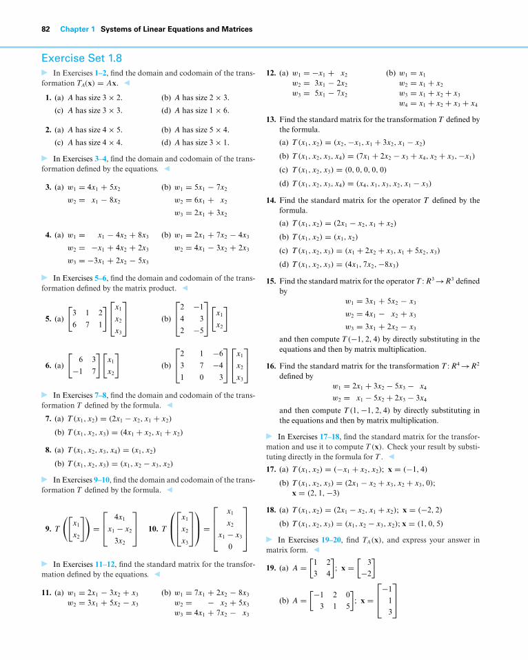
82 Chapter 1 Systems of Linear Equations and Matrices
Exercise Set 1.8In Exercises 1–2, find the domain and codomain of the trans-
formation TA(x) = Ax.
1. (a) A has size 3 × 2. (b) A has size 2 × 3.
(c) A has size 3 × 3. (d) A has size 1 × 6.
2. (a) A has size 4 × 5. (b) A has size 5 × 4.
(c) A has size 4 × 4. (d) A has size 3 × 1.
In Exercises 3–4, find the domain and codomain of the trans-formation defined by the equations.
3. (a) w1 = 4x1 + 5x2
w2 = x1 − 8x2
(b) w1 = 5x1 − 7x2
w2 = 6x1 + x2
w3 = 2x1 + 3x2
4. (a) w1 = x1 − 4x2 + 8x3
w2 = −x1 + 4x2 + 2x3
w3 = −3x1 + 2x2 − 5x3
(b) w1 = 2x1 + 7x2 − 4x3
w2 = 4x1 − 3x2 + 2x3
In Exercises 5–6, find the domain and codomain of the trans-formation defined by the matrix product.
5. (a)
[3 1 2
6 7 1
]⎡⎢⎣x1
x2
x3
⎤⎥⎦ (b)
⎡⎢⎣2 −1
4 3
2 −5
⎤⎥⎦[x1
x2
]
6. (a)
[6 3
−1 7
][x1
x2
](b)
⎡⎢⎣2 1 −6
3 7 −4
1 0 3
⎤⎥⎦⎡⎢⎣x1
x2
x3
⎤⎥⎦
In Exercises 7–8, find the domain and codomain of the trans-formation T defined by the formula.
7. (a) T (x1, x2) = (2x1 − x2, x1 + x2)
(b) T (x1, x2, x3) = (4x1 + x2, x1 + x2)
8. (a) T (x1, x2, x3, x4) = (x1, x2)
(b) T (x1, x2, x3) = (x1, x2 − x3, x2)
In Exercises 9–10, find the domain and codomain of the trans-formation T defined by the formula.
9. T
([x1
x2
])=⎡⎢⎣ 4x1
x1 − x2
3x2
⎤⎥⎦ 10. T
⎛⎜⎝⎡⎢⎣x1
x2
x3
⎤⎥⎦⎞⎟⎠ =
⎡⎢⎢⎢⎣
x1
x2
x1 − x3
0
⎤⎥⎥⎥⎦
In Exercises 11–12, find the standard matrix for the transfor-mation defined by the equations.
11. (a) w1 = 2x1 − 3x2 + x3
w2 = 3x1 + 5x2 − x3
(b) w1 = 7x1 + 2x2 − 8x3
w2 = − x2 + 5x3
w3 = 4x1 + 7x2 − x3
12. (a) w1 = −x1 + x2
w2 = 3x1 − 2x2
w3 = 5x1 − 7x2
(b) w1 = x1
w2 = x1 + x2
w3 = x1 + x2 + x3
w4 = x1 + x2 + x3 + x4
13. Find the standard matrix for the transformation T defined bythe formula.
(a) T (x1, x2) = (x2,−x1, x1 + 3x2, x1 − x2)
(b) T (x1, x2, x3, x4) = (7x1 + 2x2 − x3 + x4, x2 + x3,−x1)
(c) T (x1, x2, x3) = (0, 0, 0, 0, 0)
(d) T (x1, x2, x3, x4) = (x4, x1, x3, x2, x1 − x3)
14. Find the standard matrix for the operator T defined by theformula.
(a) T (x1, x2) = (2x1 − x2, x1 + x2)
(b) T (x1, x2) = (x1, x2)
(c) T (x1, x2, x3) = (x1 + 2x2 + x3, x1 + 5x2, x3)
(d) T (x1, x2, x3) = (4x1, 7x2,−8x3)
15. Find the standard matrix for the operator T : R3 →R3 definedby
w1 = 3x1 + 5x2 − x3
w2 = 4x1 − x2 + x3
w3 = 3x1 + 2x2 − x3
and then compute T (−1, 2, 4) by directly substituting in theequations and then by matrix multiplication.
16. Find the standard matrix for the transformation T : R4 →R2
defined byw1 = 2x1 + 3x2 − 5x3 − x4
w2 = x1 − 5x2 + 2x3 − 3x4
and then compute T (1,−1, 2, 4) by directly substituting inthe equations and then by matrix multiplication.
In Exercises 17–18, find the standard matrix for the transfor-mation and use it to compute T (x). Check your result by substi-tuting directly in the formula for T .
17. (a) T (x1, x2) = (−x1 + x2, x2); x = (−1, 4)
(b) T (x1, x2, x3) = (2x1 − x2 + x3, x2 + x3, 0);x = (2, 1,−3)
18. (a) T (x1, x2) = (2x1 − x2, x1 + x2); x = (−2, 2)
(b) T (x1, x2, x3) = (x1, x2 − x3, x2); x = (1, 0, 5)
In Exercises 19–20, find TA(x), and express your answer inmatrix form.
19. (a) A =[
1 2
3 4
]; x =
[3
−2
]
(b) A =[−1 2 0
3 1 5
]; x =
⎡⎢⎣−1
1
3
⎤⎥⎦
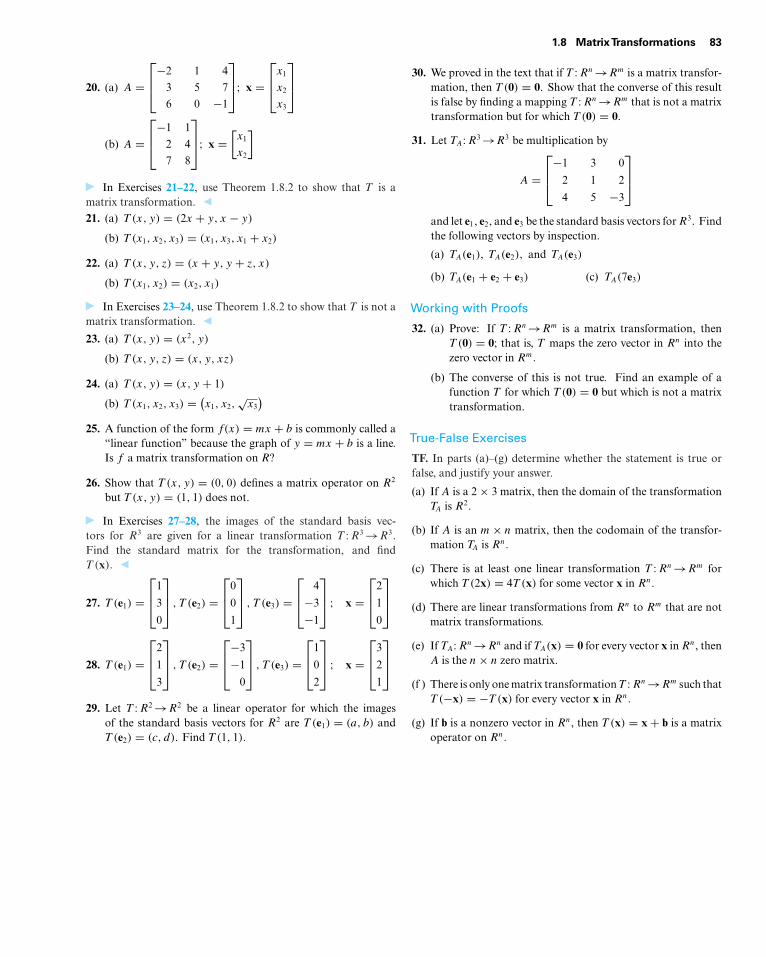
1.8 MatrixTransformations 83
20. (a) A =⎡⎢⎣−2 1 4
3 5 7
6 0 −1
⎤⎥⎦; x =
⎡⎢⎣x1
x2
x3
⎤⎥⎦
(b) A =⎡⎢⎣−1 1
2 4
7 8
⎤⎥⎦; x =
[x1
x2
]
In Exercises 21–22, use Theorem 1.8.2 to show that T is amatrix transformation.21. (a) T (x, y) = (2x + y, x − y)
(b) T (x1, x2, x3) = (x1, x3, x1 + x2)
22. (a) T (x, y, z) = (x + y, y + z, x)
(b) T (x1, x2) = (x2, x1)
In Exercises 23–24, use Theorem 1.8.2 to show that T is not amatrix transformation.
23. (a) T (x, y) = (x2, y)
(b) T (x, y, z) = (x, y, xz)
24. (a) T (x, y) = (x, y + 1)
(b) T (x1, x2, x3) = (x1, x2,
√x3
)25. A function of the form f(x) = mx + b is commonly called a
“linear function” because the graph of y = mx + b is a line.Is f a matrix transformation on R?
26. Show that T (x, y) = (0, 0) defines a matrix operator on R2
but T (x, y) = (1, 1) does not.
In Exercises 27–28, the images of the standard basis vec-tors for R3 are given for a linear transformation T : R3 →R3.Find the standard matrix for the transformation, and findT (x).
27. T (e1) =⎡⎢⎣1
3
0
⎤⎥⎦ , T (e2) =
⎡⎢⎣0
0
1
⎤⎥⎦ , T (e3) =
⎡⎢⎣ 4
−3
−1
⎤⎥⎦ ; x =
⎡⎢⎣2
1
0
⎤⎥⎦
28. T (e1) =⎡⎢⎣2
1
3
⎤⎥⎦ , T (e2) =
⎡⎢⎣−3
−1
0
⎤⎥⎦ , T (e3) =
⎡⎢⎣1
0
2
⎤⎥⎦ ; x =
⎡⎢⎣3
2
1
⎤⎥⎦
29. Let T : R2 →R2 be a linear operator for which the imagesof the standard basis vectors for R2 are T (e1) = (a, b) andT (e2) = (c, d). Find T (1, 1).
30. We proved in the text that if T : Rn →Rm is a matrix transfor-mation, then T (0) = 0. Show that the converse of this resultis false by finding a mapping T : Rn →Rm that is not a matrixtransformation but for which T (0) = 0.
31. Let TA: R3 →R3 be multiplication by
A =⎡⎢⎣−1 3 0
2 1 2
4 5 −3
⎤⎥⎦
and let e1, e2, and e3 be the standard basis vectors for R3. Findthe following vectors by inspection.
(a) TA(e1), TA(e2), and TA(e3)
(b) TA(e1 + e2 + e3) (c) TA(7e3)
Working with Proofs
32. (a) Prove: If T : Rn →Rm is a matrix transformation, thenT (0) = 0; that is, T maps the zero vector in Rn into thezero vector in Rm.
(b) The converse of this is not true. Find an example of afunction T for which T (0) = 0 but which is not a matrixtransformation.
True-False Exercises
TF. In parts (a)–(g) determine whether the statement is true orfalse, and justify your answer.
(a) If A is a 2 × 3 matrix, then the domain of the transformationTA is R2.
(b) If A is an m × n matrix, then the codomain of the transfor-mation TA is Rn.
(c) There is at least one linear transformation T : Rn →Rm forwhich T (2x) = 4T (x) for some vector x in Rn.
(d) There are linear transformations from Rn to Rm that are notmatrix transformations.
(e) If TA: Rn →Rn and if TA(x) = 0 for every vector x in Rn, thenA is the n × n zero matrix.
(f ) There is only one matrix transformation T : Rn →Rm such thatT (−x) = −T (x) for every vector x in Rn.
(g) If b is a nonzero vector in Rn, then T (x) = x + b is a matrixoperator on Rn.
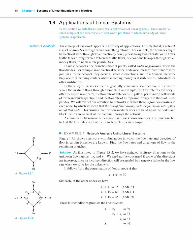
84 Chapter 1 Systems of Linear Equations and Matrices
1.9 Applications of Linear SystemsIn this section we will discuss some brief applications of linear systems. These are but asmall sample of the wide variety of real-world problems to which our study of linearsystems is applicable.
Network Analysis The concept of a network appears in a variety of applications. Loosely stated, a networkis a set of branches through which something “flows.” For example, the branches mightbe electrical wires through which electricity flows, pipes through which water or oil flows,traffic lanes through which vehicular traffic flows, or economic linkages through whichmoney flows, to name a few possibilities.
In most networks, the branches meet at points, called nodes or junctions, where theflow divides. For example, in an electrical network, nodes occur where three or more wiresjoin, in a traffic network they occur at street intersections, and in a financial networkthey occur at banking centers where incoming money is distributed to individuals orother institutions.
In the study of networks, there is generally some numerical measure of the rate atwhich the medium flows through a branch. For example, the flow rate of electricity isoften measured in amperes, the flow rate of water or oil in gallons per minute, the flow rateof traffic in vehicles per hour, and the flow rate of European currency in millions of Eurosper day. We will restrict our attention to networks in which there is flow conservation ateach node, by which we mean that the rate of flow into any node is equal to the rate of flowout of that node. This ensures that the flow medium does not build up at the nodes andblock the free movement of the medium through the network.
A common problem in network analysis is to use known flow rates in certain branchesto find the flow rates in all of the branches. Here is an example.
EXAMPLE 1 Network Analysis Using Linear Systems
Figure 1.9.1 shows a network with four nodes in which the flow rate and direction of
35
30
55
60
15
Figure 1.9.1
flow in certain branches are known. Find the flow rates and directions of flow in theremaining branches.
Solution As illustrated in Figure 1.9.2, we have assigned arbitrary directions to the
35
30
55
60
15
x1x2
x3
B
A
D
C
Figure 1.9.2
unknown flow rates x1, x2, and x3. We need not be concerned if some of the directionsare incorrect, since an incorrect direction will be signaled by a negative value for the flowrate when we solve for the unknowns.
It follows from the conservation of flow at node A that
x1 + x2 = 30
Similarly, at the other nodes we have
x2 + x3 = 35 (node B)
x3 + 15 = 60 (node C)
x1 + 15 = 55 (node D)
These four conditions produce the linear system
x1 + x2 = 30
x2 + x3 = 35
x3 = 45
x1 = 40
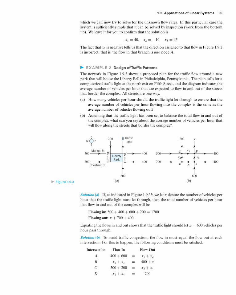
1.9 Applications of Linear Systems 85
which we can now try to solve for the unknown flow rates. In this particular case thesystem is sufficiently simple that it can be solved by inspection (work from the bottomup). We leave it for you to confirm that the solution is
x1 = 40, x2 = −10, x3 = 45
The fact that x2 is negative tells us that the direction assigned to that flow in Figure 1.9.2is incorrect; that is, the flow in that branch is into node A.
EXAMPLE 2 Design ofTraffic Patterns
The network in Figure 1.9.3 shows a proposed plan for the traffic flow around a newpark that will house the Liberty Bell in Philadelphia, Pennsylvania. The plan calls for acomputerized traffic light at the north exit on Fifth Street, and the diagram indicates theaverage number of vehicles per hour that are expected to flow in and out of the streetsthat border the complex. All streets are one-way.
(a) How many vehicles per hour should the traffic light let through to ensure that theaverage number of vehicles per hour flowing into the complex is the same as theaverage number of vehicles flowing out?
(b) Assuming that the traffic light has been set to balance the total flow in and out ofthe complex, what can you say about the average number of vehicles per hour thatwill flow along the streets that border the complex?
Figure 1.9.3
N
W E
S
Liberty
Park
Market St.
Chestnut St.
400
400
600
500
200
700
Traffic
light
400
400
600
500
200
700AD
C B
x1
x2
x
x3
x4
(a) (b)
Six
th S
t.
Fif
th S
t.
Solution (a) If, as indicated in Figure 1.9.3b, we let x denote the number of vehicles perhour that the traffic light must let through, then the total number of vehicles per hourthat flow in and out of the complex will be
Flowing in: 500 + 400 + 600 + 200 = 1700
Flowing out: x + 700 + 400
Equating the flows in and out shows that the traffic light should let x = 600 vehicles perhour pass through.
Solution (b) To avoid traffic congestion, the flow in must equal the flow out at eachintersection. For this to happen, the following conditions must be satisfied:
Intersection Flow In Flow Out
A 400 + 600 = x1 + x2
B x2 + x3 = 400 + x
C 500 + 200 = x3 + x4
D x1 + x4 = 700
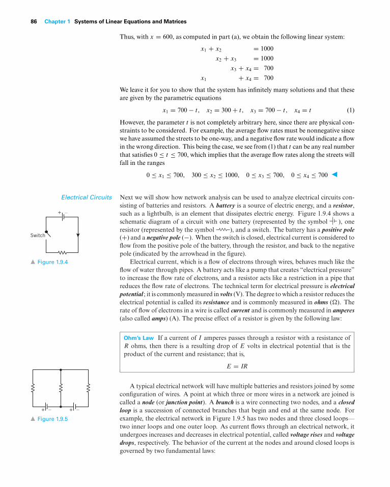
86 Chapter 1 Systems of Linear Equations and Matrices
Thus, with x = 600, as computed in part (a), we obtain the following linear system:
x1 + x2 = 1000
x2 + x3 = 1000
x3 + x4 = 700
x1 + x4 = 700
We leave it for you to show that the system has infinitely many solutions and that theseare given by the parametric equations
x1 = 700 − t, x2 = 300 + t, x3 = 700 − t, x4 = t (1)
However, the parameter t is not completely arbitrary here, since there are physical con-straints to be considered. For example, the average flow rates must be nonnegative sincewe have assumed the streets to be one-way, and a negative flow rate would indicate a flowin the wrong direction. This being the case, we see from (1) that t can be any real numberthat satisfies 0 ≤ t ≤ 700, which implies that the average flow rates along the streets willfall in the ranges
0 ≤ x1 ≤ 700, 300 ≤ x2 ≤ 1000, 0 ≤ x3 ≤ 700, 0 ≤ x4 ≤ 700
Electrical Circuits Next we will show how network analysis can be used to analyze electrical circuits con-sisting of batteries and resistors. A battery is a source of electric energy, and a resistor,such as a lightbulb, is an element that dissipates electric energy. Figure 1.9.4 shows a+ –
Switch
Figure 1.9.4
schematic diagram of a circuit with one battery (represented by the symbol ), oneresistor (represented by the symbol ), and a switch. The battery has a positive pole(+) and a negative pole (−). When the switch is closed, electrical current is considered toflow from the positive pole of the battery, through the resistor, and back to the negativepole (indicated by the arrowhead in the figure).
Electrical current, which is a flow of electrons through wires, behaves much like theflow of water through pipes. A battery acts like a pump that creates “electrical pressure”to increase the flow rate of electrons, and a resistor acts like a restriction in a pipe thatreduces the flow rate of electrons. The technical term for electrical pressure is electricalpotential ; it is commonly measured in volts (V). The degree to which a resistor reduces theelectrical potential is called its resistance and is commonly measured in ohms (�). Therate of flow of electrons in a wire is called current and is commonly measured in amperes(also called amps) (A). The precise effect of a resistor is given by the following law:
Ohm’s Law If a current of I amperes passes through a resistor with a resistance ofR ohms, then there is a resulting drop of E volts in electrical potential that is theproduct of the current and resistance; that is,
E = IR
A typical electrical network will have multiple batteries and resistors joined by someconfiguration of wires. A point at which three or more wires in a network are joined iscalled a node (or junction point). A branch is a wire connecting two nodes, and a closedloop is a succession of connected branches that begin and end at the same node. Forexample, the electrical network in Figure 1.9.5 has two nodes and three closed loops—
+ – + –
Figure 1.9.5
two inner loops and one outer loop. As current flows through an electrical network, itundergoes increases and decreases in electrical potential, called voltage rises and voltagedrops, respectively. The behavior of the current at the nodes and around closed loops isgoverned by two fundamental laws:
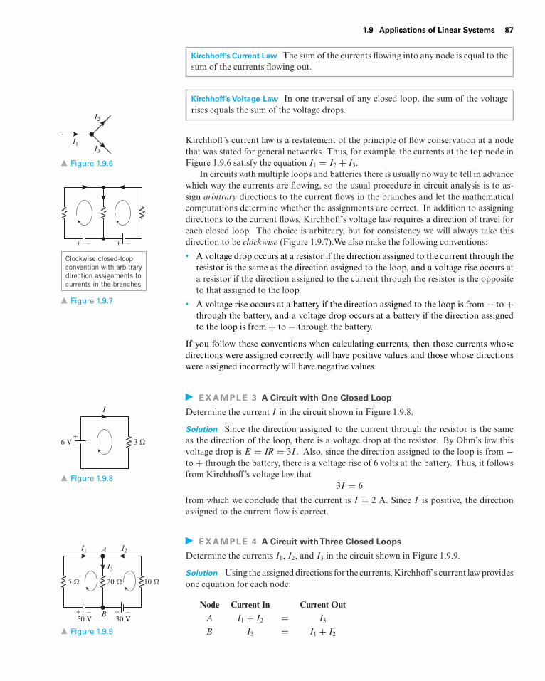
1.9 Applications of Linear Systems 87
Kirchhoff’s Current Law The sum of the currents flowing into any node is equal to thesum of the currents flowing out.
Kirchhoff’s Voltage Law In one traversal of any closed loop, the sum of the voltagerises equals the sum of the voltage drops.
Kirchhoff’s current law is a restatement of the principle of flow conservation at a nodethat was stated for general networks. Thus, for example, the currents at the top node inFigure 1.9.6 satisfy the equation I1 = I2 + I3.
I3
I2
I1
Figure 1.9.6
In circuits with multiple loops and batteries there is usually no way to tell in advancewhich way the currents are flowing, so the usual procedure in circuit analysis is to as-sign arbitrary directions to the current flows in the branches and let the mathematicalcomputations determine whether the assignments are correct. In addition to assigningdirections to the current flows, Kirchhoff’s voltage law requires a direction of travel foreach closed loop. The choice is arbitrary, but for consistency we will always take thisdirection to be clockwise (Figure 1.9.7).We also make the following conventions:
• A voltage drop occurs at a resistor if the direction assigned to the current through theresistor is the same as the direction assigned to the loop, and a voltage rise occurs at
+ – + –
Clockwise closed-loop
convention with arbitrary
direction assignments to
currents in the branches
Figure 1.9.7
a resistor if the direction assigned to the current through the resistor is the oppositeto that assigned to the loop.
• A voltage rise occurs at a battery if the direction assigned to the loop is from − to +through the battery, and a voltage drop occurs at a battery if the direction assignedto the loop is from + to − through the battery.
If you follow these conventions when calculating currents, then those currents whosedirections were assigned correctly will have positive values and those whose directionswere assigned incorrectly will have negative values.
EXAMPLE 3 A Circuit with One Closed Loop
Determine the current I in the circuit shown in Figure 1.9.8.
+– 3 �6 V
I
Figure 1.9.8
Solution Since the direction assigned to the current through the resistor is the sameas the direction of the loop, there is a voltage drop at the resistor. By Ohm’s law thisvoltage drop is E = IR = 3I . Also, since the direction assigned to the loop is from −to + through the battery, there is a voltage rise of 6 volts at the battery. Thus, it followsfrom Kirchhoff’s voltage law that
3I = 6
from which we conclude that the current is I = 2 A. Since I is positive, the directionassigned to the current flow is correct.
EXAMPLE 4 A Circuit withThree Closed Loops
Determine the currents I1, I2, and I3 in the circuit shown in Figure 1.9.9.
+ – + –
5 � 20 � 10 �
50 V 30 V
AI1 I2
I3
B
Figure 1.9.9
Solution Using the assigned directions for the currents, Kirchhoff’s current law providesone equation for each node:
Node Current In Current OutA I1 + I2 = I3
B I3 = I1 + I2
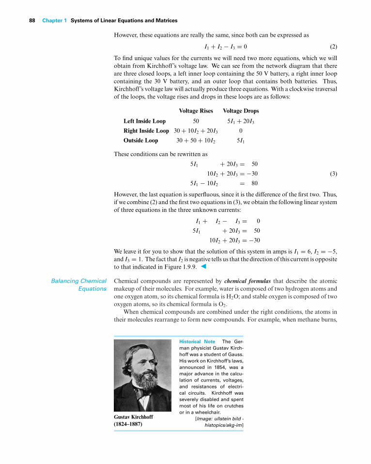
88 Chapter 1 Systems of Linear Equations and Matrices
However, these equations are really the same, since both can be expressed as
I1 + I2 − I3 = 0 (2)
To find unique values for the currents we will need two more equations, which we willobtain from Kirchhoff’s voltage law. We can see from the network diagram that thereare three closed loops, a left inner loop containing the 50 V battery, a right inner loopcontaining the 30 V battery, and an outer loop that contains both batteries. Thus,Kirchhoff’s voltage law will actually produce three equations. With a clockwise traversalof the loops, the voltage rises and drops in these loops are as follows:
Voltage Rises Voltage Drops
Left Inside Loop 50 5I1 + 20I3
Right Inside Loop 30 + 10I2 + 20I3 0
Outside Loop 30 + 50 + 10I2 5I1
These conditions can be rewritten as
5I1 + 20I3 = 50
10I2 + 20I3 = −30
5I1 − 10I2 = 80
(3)
However, the last equation is superfluous, since it is the difference of the first two. Thus,if we combine (2) and the first two equations in (3), we obtain the following linear systemof three equations in the three unknown currents:
I1 + I2 − I3 = 0
5I1 + 20I3 = 50
10I2 + 20I3 = −30
We leave it for you to show that the solution of this system in amps is I1 = 6, I2 = −5,and I3 = 1. The fact that I2 is negative tells us that the direction of this current is oppositeto that indicated in Figure 1.9.9.
Balancing ChemicalEquations
Chemical compounds are represented by chemical formulas that describe the atomicmakeup of their molecules. For example, water is composed of two hydrogen atoms andone oxygen atom, so its chemical formula is H2O; and stable oxygen is composed of twooxygen atoms, so its chemical formula is O2.
When chemical compounds are combined under the right conditions, the atoms intheir molecules rearrange to form new compounds. For example, when methane burns,
Gustav Kirchhoff(1824–1887)
Historical Note The Ger-man physicist Gustav Kirch-hoff was a student of Gauss.His work on Kirchhoff’s laws,announced in 1854, was amajor advance in the calcu-lation of currents, voltages,and resistances of electri-cal circuits. Kirchhoff wasseverely disabled and spentmost of his life on crutchesor in a wheelchair.
[Image: ullstein bild -histopics/akg-im]
1.9 Applications of Linear Systems 89
the methane (CH4) and stable oxygen (O2) react to form carbon dioxide (CO2) and water(H2O). This is indicated by the chemical equation
CH4 + O2 −→ CO2 + H2O (4)
The molecules to the left of the arrow are called the reactants and those to the rightthe products. In this equation the plus signs serve to separate the molecules and arenot intended as algebraic operations. However, this equation does not tell the wholestory, since it fails to account for the proportions of molecules required for a completereaction (no reactants left over). For example, we can see from the right side of (4) thatto produce one molecule of carbon dioxide and one molecule of water, one needs threeoxygen atoms for each carbon atom. However, from the left side of (4) we see that onemolecule of methane and one molecule of stable oxygen have only two oxygen atomsfor each carbon atom. Thus, on the reactant side the ratio of methane to stable oxygencannot be one-to-one in a complete reaction.
A chemical equation is said to be balanced if for each type of atom in the reaction,the same number of atoms appears on each side of the arrow. For example, the balancedversion of Equation (4) is
CH4 + 2O2 −→ CO2 + 2H2O (5)
by which we mean that one methane molecule combines with two stable oxygen moleculesto produce one carbon dioxide molecule and two water molecules. In theory, one couldmultiply this equation through by any positive integer. For example, multiplying throughby 2 yields the balanced chemical equation
2CH4 + 4O2 −→ 2CO2 + 4H2O
However, the standard convention is to use the smallest positive integers that will balancethe equation.
Equation (4) is sufficiently simple that it could have been balanced by trial and error,but for more complicated chemical equations we will need a systematic method. Thereare various methods that can be used, but we will give one that uses systems of linearequations. To illustrate the method let us reexamine Equation (4). To balance thisequation we must find positive integers, x1, x2, x3, and x4 such that
x1 (CH4) + x2 (O2) −→ x3 (CO2) + x4 (H2O) (6)
For each of the atoms in the equation, the number of atoms on the left must be equal tothe number of atoms on the right. Expressing this in tabular form we have
Left Side Right SideCarbon x1 = x3
Hydrogen 4x1 = 2x4
Oxygen 2x2 = 2x3 + x4
from which we obtain the homogeneous linear system
x1 − x3 = 0
4x1 − 2x4 = 0
2x2 − 2x3 − x4 = 0
The augmented matrix for this system is⎡⎢⎣1 0 −1 0 0
4 0 0 −2 0
0 2 −2 −1 0
⎤⎥⎦
90 Chapter 1 Systems of Linear Equations and Matrices
We leave it for you to show that the reduced row echelon form of this matrix is⎡⎢⎣
1 0 0 − 12 0
0 1 0 −1 0
0 0 1 − 12 0
⎤⎥⎦
from which we conclude that the general solution of the system is
x1 = t/2, x2 = t, x3 = t/2, x4 = t
where t is arbitrary. The smallest positive integer values for the unknowns occur whenwe let t = 2, so the equation can be balanced by letting x1 = 1, x2 = 2, x3 = 1, x4 = 2.This agrees with our earlier conclusions, since substituting these values into Equation (6)yields Equation (5).
EXAMPLE 5 Balancing Chemical Equations Using Linear Systems
Balance the chemical equation
HCl + Na3PO4 −→ H3PO4 + NaCl
[hydrochloric acid] + [sodium phosphate] −→ [phosphoric acid] + [sodium chloride]
Solution Let x1, x2, x3, and x4 be positive integers that balance the equation
x1 (HCl) + x2 (Na3PO4) −→ x3 (H3PO4) + x4 (NaCl) (7)
Equating the number of atoms of each type on the two sides yields
1x1 = 3x3 Hydrogen (H)
1x1 = 1x4 Chlorine (Cl)
3x2 = 1x4 Sodium (Na)
1x2 = 1x3 Phosphorus (P)
4x2 = 4x3 Oxygen (O)
from which we obtain the homogeneous linear system
x1 − 3x3 = 0
x1 − x4 = 0
3x2 − x4 = 0
x2 − x3 = 0
4x2 − 4x3 = 0
We leave it for you to show that the reduced row echelon form of the augmented matrixfor this system is ⎡
⎢⎢⎢⎢⎢⎢⎢⎣
1 0 0 −1 0
0 1 0 − 13 0
0 0 1 − 13 0
0 0 0 0 0
0 0 0 0 0
⎤⎥⎥⎥⎥⎥⎥⎥⎦
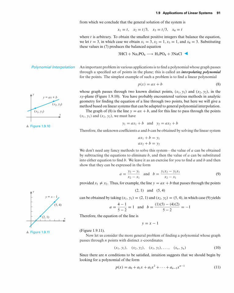
1.9 Applications of Linear Systems 91
from which we conclude that the general solution of the system is
x1 = t, x2 = t/3, x3 = t/3, x4 = t
where t is arbitrary. To obtain the smallest positive integers that balance the equation,we let t = 3, in which case we obtain x1 = 3, x2 = 1, x3 = 1, and x4 = 3. Substitutingthese values in (7) produces the balanced equation
3HCl + Na3PO4 −→ H3PO4 + 3NaCl
Polynomial Interpolation An important problem in various applications is to find a polynomial whose graph passesthrough a specified set of points in the plane; this is called an interpolating polynomialfor the points. The simplest example of such a problem is to find a linear polynomial
p(x) = ax + b (8)
whose graph passes through two known distinct points, (x1, y1) and (x2, y2), in thexy-plane (Figure 1.9.10). You have probably encountered various methods in analyticgeometry for finding the equation of a line through two points, but here we will give amethod based on linear systems that can be adapted to general polynomial interpolation.
The graph of (8) is the line y = ax + b, and for this line to pass through the pointsx
y
(x2, y2)
(x1, y1)
y = ax + b
Figure 1.9.10
(x1, y1) and (x2, y2), we must have
y1 = ax1 + b and y2 = ax2 + b
Therefore, the unknown coefficients a and b can be obtained by solving the linear system
ax1 + b = y1
ax2 + b = y2
We don’t need any fancy methods to solve this system—the value of a can be obtainedby subtracting the equations to eliminate b, and then the value of a can be substitutedinto either equation to find b. We leave it as an exercise for you to find a and b and thenshow that they can be expressed in the form
a = y2 − y1
x2 − x1and b = y1x2 − y2x1
x2 − x1(9)
provided x1 �= x2. Thus, for example, the line y = ax + b that passes through the points
(2, 1) and (5, 4)
can be obtained by taking (x1, y1) = (2, 1) and (x2, y2) = (5, 4), in which case (9) yields
a = 4 − 1
5 − 2= 1 and b = (1)(5) − (4)(2)
5 − 2= −1
Therefore, the equation of the line is
y = x − 1
(Figure 1.9.11).
y = x – 1
x
y
(2, 1)
(5, 4)
Figure 1.9.11Now let us consider the more general problem of finding a polynomial whose graph
passes through n points with distinct x-coordinates
(x1, y1), (x2, y2), (x3, y3), . . . , (xn, yn) (10)
Since there are n conditions to be satisfied, intuition suggests that we should begin bylooking for a polynomial of the form
p(x) = a0 + a1x + a2x2 + · · · + an−1x
n−1 (11)
92 Chapter 1 Systems of Linear Equations and Matrices
since a polynomial of this form has n coefficients that are at our disposal to satisfy then conditions. However, we want to allow for cases where the points may lie on a line orhave some other configuration that would make it possible to use a polynomial whosedegree is less than n − 1; thus, we allow for the possibility that an−1 and other coefficientsin (11) may be zero.
The following theorem, which we will prove later in the text, is the basic result onpolynomial interpolation.
THEOREM 1.9.1 Polynomial Interpolation
Given any n points in the xy-plane that have distinct x-coordinates, there is a uniquepolynomial of degree n − 1 or less whose graph passes through those points.
Let us now consider how we might go about finding the interpolating polynomial(11) whose graph passes through the points in (10). Since the graph of this polynomialis the graph of the equation
y = a0 + a1x + a2x2 + · · · + an−1x
n−1 (12)
it follows that the coordinates of the points must satisfy
a0 + a1x1 + a2x21 + · · ·+ an−1x
n−11 = y1
a0 + a1x2 + a2x22 + · · ·+ an−1x
n−12 = y2
......
......
...
a0 + a1xn + a2x2n + · · ·+ an−1x
n−1n = yn
(13)
In these equations the values of x’s and y’s are assumed to be known, so we can viewthis as a linear system in the unknowns a0, a1, . . . , an−1. From this point of view theaugmented matrix for the system is⎡
⎢⎢⎢⎢⎢⎢⎣
1 x1 x21 · · · xn−1
1 y1
1 x2 x22 · · · xn−1
2 y2...
......
......
1 xn x2n · · · xn−1
n yn
⎤⎥⎥⎥⎥⎥⎥⎦ (14)
and hence the interpolating polynomial can be found by reducing this matrix to reducedrow echelon form (Gauss–Jordan elimination).
EXAMPLE 6 Polynomial Interpolation by Gauss–Jordan Elimination
Find a cubic polynomial whose graph passes through the points
(1, 3), (2,−2), (3,−5), (4, 0)
Solution Since there are four points, we will use an interpolating polynomial of degreen = 3. Denote this polynomial by
p(x) = a0 + a1x + a2x2 + a3x
3
and denote the x- and y-coordinates of the given points by
x1 = 1, x2 = 2, x3 = 3, x4 = 4 and y1 = 3, y2 = −2, y3 = −5, y4 = 0
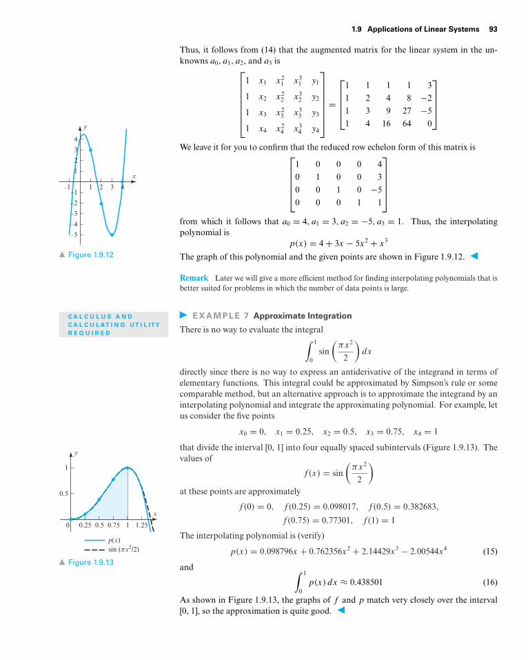
1.9 Applications of Linear Systems 93
Thus, it follows from (14) that the augmented matrix for the linear system in the un-knowns a0, a1, a2, and a3 is⎡
⎢⎢⎢⎢⎢⎢⎣
1 x1 x21 x3
1 y1
1 x2 x22 x3
2 y2
1 x3 x23 x3
3 y3
1 x4 x24 x3
4 y4
⎤⎥⎥⎥⎥⎥⎥⎦ =
⎡⎢⎢⎢⎣
1 1 1 1 3
1 2 4 8 −2
1 3 9 27 −5
1 4 16 64 0
⎤⎥⎥⎥⎦
We leave it for you to confirm that the reduced row echelon form of this matrix is⎡⎢⎢⎢⎢⎣
1 0 0 0 4
0 1 0 0 3
0 0 1 0 −5
0 0 0 1 1
⎤⎥⎥⎥⎥⎦
from which it follows that a0 = 4, a1 = 3, a2 = −5, a3 = 1. Thus, the interpolatingpolynomial is
p(x) = 4 + 3x − 5x2 + x3
The graph of this polynomial and the given points are shown in Figure 1.9.12.
–1 1 2 3 4
–5
–4
–3
–2
–1
1
2
3
4
x
y
Figure 1.9.12
Remark Later we will give a more efficient method for finding interpolating polynomials that isbetter suited for problems in which the number of data points is large.
EXAMPLE 7 Approximate IntegrationCA L C U L U S A N DCA L C U LAT I N G UT I L ITYR E Q U I R E D There is no way to evaluate the integral∫ 1
0sin
(πx2
2
)dx
directly since there is no way to express an antiderivative of the integrand in terms ofelementary functions. This integral could be approximated by Simpson’s rule or somecomparable method, but an alternative approach is to approximate the integrand by aninterpolating polynomial and integrate the approximating polynomial. For example, letus consider the five points
x0 = 0, x1 = 0.25, x2 = 0.5, x3 = 0.75, x4 = 1
that divide the interval [0, 1] into four equally spaced subintervals (Figure 1.9.13). The
0.250 0.5 0.75 1 1.25
0.5
1
x
y
sin (πx2/2)p(x)
Figure 1.9.13
values of
f(x) = sin
(πx2
2
)at these points are approximately
f(0) = 0, f(0.25) = 0.098017, f(0.5) = 0.382683,
f(0.75) = 0.77301, f(1) = 1
The interpolating polynomial is (verify)
p(x) = 0.098796x + 0.762356x2 + 2.14429x3 − 2.00544x4 (15)
and ∫ 1
0p(x) dx ≈ 0.438501 (16)
As shown in Figure 1.9.13, the graphs of f and p match very closely over the interval[0, 1], so the approximation is quite good.
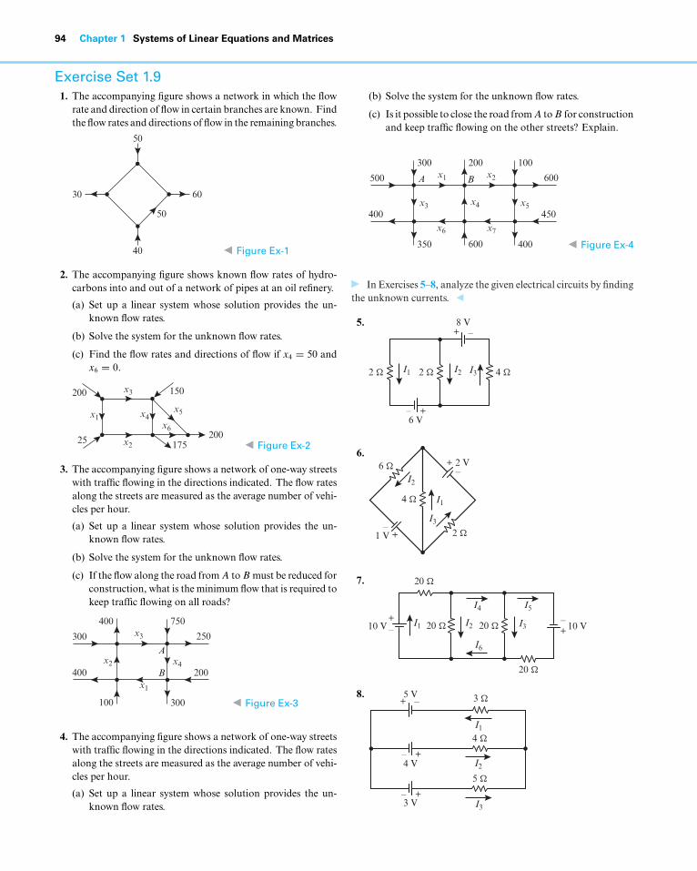
94 Chapter 1 Systems of Linear Equations and Matrices
Exercise Set 1.91. The accompanying figure shows a network in which the flow
rate and direction of flow in certain branches are known. Findthe flow rates and directions of flow in the remaining branches.
30
50
60
40
50
Figure Ex-1
2. The accompanying figure shows known flow rates of hydro-carbons into and out of a network of pipes at an oil refinery.
(a) Set up a linear system whose solution provides the un-known flow rates.
(b) Solve the system for the unknown flow rates.
(c) Find the flow rates and directions of flow if x4 = 50 andx6 = 0.
200
25 200175
150
x1 x4x5
x6
x3
x2 Figure Ex-2
3. The accompanying figure shows a network of one-way streetswith traffic flowing in the directions indicated. The flow ratesalong the streets are measured as the average number of vehi-cles per hour.
(a) Set up a linear system whose solution provides the un-known flow rates.
(b) Solve the system for the unknown flow rates.
(c) If the flow along the road from A to B must be reduced forconstruction, what is the minimum flow that is required tokeep traffic flowing on all roads?
300
400 200
250
750
300
400
100
x2 x4
x3
x1
A
B
Figure Ex-3
4. The accompanying figure shows a network of one-way streetswith traffic flowing in the directions indicated. The flow ratesalong the streets are measured as the average number of vehi-cles per hour.
(a) Set up a linear system whose solution provides the un-known flow rates.
(b) Solve the system for the unknown flow rates.
(c) Is it possible to close the road from A to B for constructionand keep traffic flowing on the other streets? Explain.
500
400 450
600
100
400
200
600
x4 x5
300
350
x3
x6
x2x1
x7
A B
Figure Ex-4
In Exercises 5–8, analyze the given electrical circuits by findingthe unknown currents.
5.
+–
–+
2 � 2 � 4 �
6 V
8 V
I1 I2 I3
6.
–
–
+
+
4 �
6 �
2 �
2 V
1 V
I1
I2
I3
7.
–+
+–
20 �
20 �
20 � 20 �10 V 10 VI1 I2
I4
I6
I3
I5
8.+ –
+–
3 �
5 �
4 �
3 V
+–4 V
5 V
I3
I1
I2
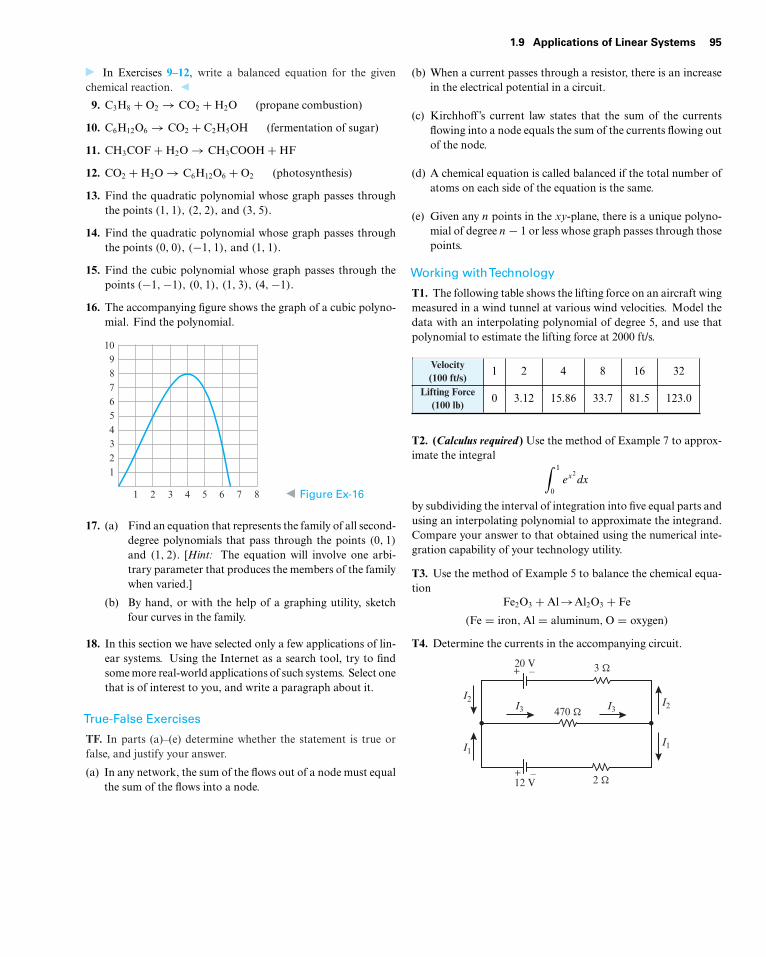
1.9 Applications of Linear Systems 95
In Exercises 9–12, write a balanced equation for the givenchemical reaction.
9. C3H8 + O2 → CO2 + H2O (propane combustion)
10. C6H12O6 → CO2 + C2H5OH (fermentation of sugar)
11. CH3COF + H2O → CH3COOH + HF
12. CO2 + H2O → C6H12O6 + O2 (photosynthesis)
13. Find the quadratic polynomial whose graph passes throughthe points (1, 1), (2, 2), and (3, 5).
14. Find the quadratic polynomial whose graph passes throughthe points (0, 0), (−1, 1), and (1, 1).
15. Find the cubic polynomial whose graph passes through thepoints (−1,−1), (0, 1), (1, 3), (4,−1).
16. The accompanying figure shows the graph of a cubic polyno-mial. Find the polynomial.
1 2 3 4 5 6 7 8
123456789
10
Figure Ex-16
17. (a) Find an equation that represents the family of all second-degree polynomials that pass through the points (0, 1)and (1, 2). [Hint: The equation will involve one arbi-trary parameter that produces the members of the familywhen varied.]
(b) By hand, or with the help of a graphing utility, sketchfour curves in the family.
18. In this section we have selected only a few applications of lin-ear systems. Using the Internet as a search tool, try to findsome more real-world applications of such systems. Select onethat is of interest to you, and write a paragraph about it.
True-False Exercises
TF. In parts (a)–(e) determine whether the statement is true orfalse, and justify your answer.
(a) In any network, the sum of the flows out of a node must equalthe sum of the flows into a node.
(b) When a current passes through a resistor, there is an increasein the electrical potential in a circuit.
(c) Kirchhoff’s current law states that the sum of the currentsflowing into a node equals the sum of the currents flowing outof the node.
(d) A chemical equation is called balanced if the total number ofatoms on each side of the equation is the same.
(e) Given any n points in the xy-plane, there is a unique polyno-mial of degree n − 1 or less whose graph passes through thosepoints.
Working withTechnology
T1. The following table shows the lifting force on an aircraft wingmeasured in a wind tunnel at various wind velocities. Model thedata with an interpolating polynomial of degree 5, and use thatpolynomial to estimate the lifting force at 2000 ft/s.
Velocity(100 ft/s)
1 2 4 8 16 32
Lifting Force(100 lb)
0 3.12 15.86 33.7 81.5 123.0
T2. (Calculus required ) Use the method of Example 7 to approx-imate the integral ∫ 1
0ex2
dx
by subdividing the interval of integration into five equal parts andusing an interpolating polynomial to approximate the integrand.Compare your answer to that obtained using the numerical inte-gration capability of your technology utility.
T3. Use the method of Example 5 to balance the chemical equa-tion
Fe2O3 + Al→Al2O3 + Fe
(Fe = iron, Al = aluminum, O = oxygen)
T4. Determine the currents in the accompanying circuit.
+ –
–+
3 �
2 �
470 �
12 V
20 V
I2
I1
I2
I1
I3I3
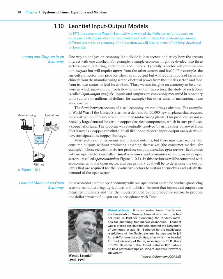
96 Chapter 1 Systems of Linear Equations and Matrices
1.10 Leontief Input-Output ModelsIn 1973 the economist Wassily Leontief was awarded the Nobel prize for his work oneconomic modeling in which he used matrix methods to study the relationships amongdifferent sectors in an economy. In this section we will discuss some of the ideas developedby Leontief.
Inputs and Outputs in anEconomy
One way to analyze an economy is to divide it into sectors and study how the sectorsinteract with one another. For example, a simple economy might be divided into threesectors—manufacturing, agriculture, and utilities. Typically, a sector will produce cer-tain outputs but will require inputs from the other sectors and itself. For example, theagricultural sector may produce wheat as an output but will require inputs of farm ma-chinery from the manufacturing sector, electrical power from the utilities sector, and foodfrom its own sector to feed its workers. Thus, we can imagine an economy to be a net-work in which inputs and outputs flow in and out of the sectors; the study of such flowsis called input-output analysis. Inputs and outputs are commonly measured in monetaryunits (dollars or millions of dollars, for example) but other units of measurement arealso possible.
The flows between sectors of a real economy are not always obvious. For example,
Manufacturing Agriculture
Utilities
Open
Sector
Figure 1.10.1
in World War II the United States had a demand for 50,000 new airplanes that requiredthe construction of many new aluminum manufacturing plants. This produced an unex-pectedly large demand for certain copper electrical components, which in turn produceda copper shortage. The problem was eventually resolved by using silver borrowed fromFort Knox as a copper substitute. In all likelihood modern input-output analysis wouldhave anticipated the copper shortage.
Most sectors of an economy will produce outputs, but there may exist sectors thatconsume outputs without producing anything themselves (the consumer market, forexample). Those sectors that do not produce outputs are called open sectors. Economieswith no open sectors are called closed economies, and economies with one or more opensectors are called open economies (Figure 1.10.1). In this section we will be concerned witheconomies with one open sector, and our primary goal will be to determine the outputlevels that are required for the productive sectors to sustain themselves and satisfy thedemand of the open sector.
Leontief Model of an OpenEconomy
Let us consider a simple open economy with one open sector and three product-producingsectors: manufacturing, agriculture, and utilities. Assume that inputs and outputs aremeasured in dollars and that the inputs required by the productive sectors to produceone dollar’s worth of output are in accordance with Table 1.
Wassily Leontief(1906–1999)
Historical Note It is somewhat ironic that it wasthe Russian-born Wassily Leontief who won the No-bel prize in 1973 for pioneering the modern meth-ods for analyzing free-market economies. Leontiefwas a precocious student who entered the Universityof Leningrad at age 15. Bothered by the intellectualrestrictions of the Soviet system, he was put in jailfor anti-Communist activities, after which he headedfor the University of Berlin, receiving his Ph.D. therein 1928. He came to the United States in 1931, wherehe held professorships at Harvard and then NewYorkUniversity.
[Image: © Bettmann/CORBIS]
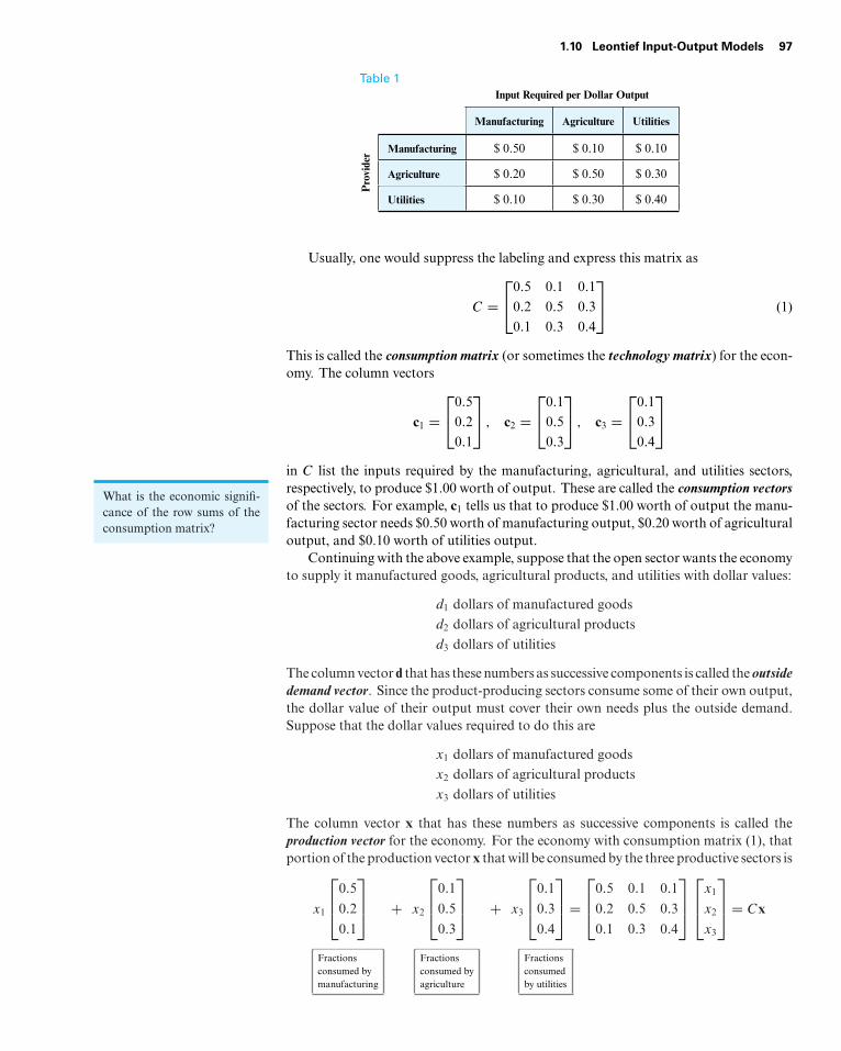
1.10 Leontief Input-Output Models 97
Table 1
Pro
vide
r
Input Required per Dollar Output
Manufacturing Agriculture Utilities
Manufacturing $ 0.50 $ 0.10 $ 0.10
Agriculture $ 0.20 $ 0.50 $ 0.30
Utilities $ 0.10 $ 0.30 $ 0.40
Usually, one would suppress the labeling and express this matrix as
C =⎡⎣0.5 0.1 0.1
0.2 0.5 0.3
0.1 0.3 0.4
⎤⎦ (1)
This is called the consumption matrix (or sometimes the technology matrix) for the econ-omy. The column vectors
c1 =⎡⎣0.5
0.2
0.1
⎤⎦ , c2 =
⎡⎣0.1
0.5
0.3
⎤⎦ , c3 =
⎡⎣0.1
0.3
0.4
⎤⎦
in C list the inputs required by the manufacturing, agricultural, and utilities sectors,respectively, to produce $1.00 worth of output. These are called the consumption vectorsof the sectors. For example, c1 tells us that to produce $1.00 worth of output the manu-facturing sector needs $0.50 worth of manufacturing output, $0.20 worth of agriculturaloutput, and $0.10 worth of utilities output.
Continuing with the above example, suppose that the open sector wants the economy
What is the economic signifi-cance of the row sums of theconsumption matrix?
to supply it manufactured goods, agricultural products, and utilities with dollar values:
d1 dollars of manufactured goods
d2 dollars of agricultural products
d3 dollars of utilities
The column vector d that has these numbers as successive components is called the outsidedemand vector. Since the product-producing sectors consume some of their own output,the dollar value of their output must cover their own needs plus the outside demand.Suppose that the dollar values required to do this are
x1 dollars of manufactured goods
x2 dollars of agricultural products
x3 dollars of utilities
The column vector x that has these numbers as successive components is called theproduction vector for the economy. For the economy with consumption matrix (1), thatportion of the production vector x that will be consumed by the three productive sectors is
x1
⎡⎢⎣0.5
0.2
0.1
⎤⎥⎦ + x2
⎡⎢⎣0.1
0.5
0.3
⎤⎥⎦ + x3
⎡⎢⎣0.1
0.3
0.4
⎤⎥⎦ =
⎡⎢⎣0.5 0.1 0.1
0.2 0.5 0.3
0.1 0.3 0.4
⎤⎥⎦⎡⎢⎣x1
x2
x3
⎤⎥⎦ = Cx
Fractionsconsumed bymanufacturing
Fractionsconsumed byagriculture
Fractionsconsumedby utilities
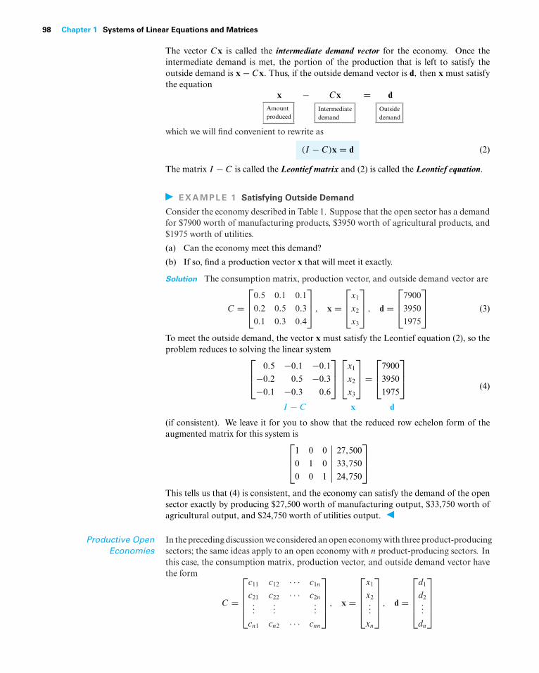
98 Chapter 1 Systems of Linear Equations and Matrices
The vector Cx is called the intermediate demand vector for the economy. Once theintermediate demand is met, the portion of the production that is left to satisfy theoutside demand is x − Cx. Thus, if the outside demand vector is d, then x must satisfythe equation
x − Cx = dAmountproduced
Intermediatedemand
Outsidedemand
which we will find convenient to rewrite as
(I − C)x = d (2)
The matrix I − C is called the Leontief matrix and (2) is called the Leontief equation.
EXAMPLE 1 Satisfying Outside Demand
Consider the economy described in Table 1. Suppose that the open sector has a demandfor $7900 worth of manufacturing products, $3950 worth of agricultural products, and$1975 worth of utilities.
(a) Can the economy meet this demand?
(b) If so, find a production vector x that will meet it exactly.
Solution The consumption matrix, production vector, and outside demand vector are
C =⎡⎢⎣0.5 0.1 0.1
0.2 0.5 0.3
0.1 0.3 0.4
⎤⎥⎦ , x =
⎡⎢⎣x1
x2
x3
⎤⎥⎦ , d =
⎡⎢⎣7900
3950
1975
⎤⎥⎦ (3)
To meet the outside demand, the vector x must satisfy the Leontief equation (2), so theproblem reduces to solving the linear system⎡
⎢⎣ 0.5 −0.1 −0.1
−0.2 0.5 −0.3
−0.1 −0.3 0.6
⎤⎥⎦⎡⎢⎣x1
x2
x3
⎤⎥⎦ =
⎡⎢⎣7900
3950
1975
⎤⎥⎦
I − C x d
(4)
(if consistent). We leave it for you to show that the reduced row echelon form of theaugmented matrix for this system is⎡
⎢⎣1 0 0 27,500
0 1 0 33,750
0 0 1 24,750
⎤⎥⎦
This tells us that (4) is consistent, and the economy can satisfy the demand of the opensector exactly by producing $27,500 worth of manufacturing output, $33,750 worth ofagricultural output, and $24,750 worth of utilities output.
Productive OpenEconomies
In the preceding discussion we considered an open economy with three product-producingsectors; the same ideas apply to an open economy with n product-producing sectors. Inthis case, the consumption matrix, production vector, and outside demand vector havethe form
C =
⎡⎢⎢⎢⎣
c11 c12 · · · c1n
c21 c22 · · · c2n...
......
cn1 cn2 · · · cnn
⎤⎥⎥⎥⎦ , x =
⎡⎢⎢⎢⎣
x1
x2...
xn
⎤⎥⎥⎥⎦ , d =
⎡⎢⎢⎢⎣
d1
d2...
dn
⎤⎥⎥⎥⎦
1.10 Leontief Input-Output Models 99
where all entries are nonnegative and
cij = the monetary value of the output of the ith sector that is needed by the j thsector to produce one unit of output
xi = the monetary value of the output of the ith sector
di = the monetary value of the output of the ith sector that is required to meetthe demand of the open sector
Remark Note that the j th column vector of C contains the monetary values that the j th sectorrequires of the other sectors to produce one monetary unit of output, and the ith row vector of C
contains the monetary values required of the ith sector by the other sectors for each of them toproduce one monetary unit of output.
As discussed in our example above, a production vector x that meets the demand dof the outside sector must satisfy the Leontief equation
(I − C)x = d
If the matrix I − C is invertible, then this equation has the unique solution
x = (I − C)−1d (5)
for every demand vector d. However, for x to be a valid production vector it musthave nonnegative entries, so the problem of importance in economics is to determineconditions under which the Leontief equation has a solution with nonnegative entries.
It is evident from the form of (5) that if I − C is invertible, and if (I − C)−1 has non-negative entries, then for every demand vector d the corresponding x will also have non-negative entries, and hence will be a valid production vector for the economy. Economiesfor which (I − C)−1 has nonnegative entries are said to be productive. Such economiesare desirable because demand can always be met by some level of production. The follow-ing theorem, whose proof can be found in many books on economics, gives conditionsunder which open economies are productive.
THEOREM 1.10.1 If C is the consumption matrix for an open economy, and if all ofthe column sums are less than 1, then the matrix I − C is invertible, the entries of(I − C)−1 are nonnegative, and the economy is productive.
Remark The j th column sum of C represents the total dollar value of input that the j th sectorrequires to produce $1 of output, so if the j th column sum is less than 1, then the j th sectorrequires less than $1 of input to produce $1 of output; in this case we say that the j th sector isprofitable. Thus, Theorem 1.10.1 states that if all product-producing sectors of an open economyare profitable, then the economy is productive. In the exercises we will ask you to show that anopen economy is productive if all of the row sums of C are less than 1 (Exercise 11). Thus, an openeconomy is productive if either all of the column sums or all of the row sums of C are less than 1.
EXAMPLE 2 An Open EconomyWhose Sectors Are All Profitable
The column sums of the consumption matrix C in (1) are less than 1, so (I − C)−1 existsand has nonnegative entries. Use a calculating utility to confirm this, and use this inverseto solve Equation (4) in Example 1.
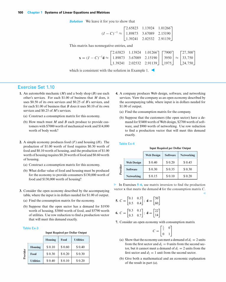
100 Chapter 1 Systems of Linear Equations and Matrices
Solution We leave it for you to show that
(I − C)−1 ≈⎡⎣2.65823 1.13924 1.01266
1.89873 3.67089 2.15190
1.39241 2.02532 2.91139
⎤⎦
This matrix has nonnegative entries, and
x = (I − C)−1d ≈⎡⎣2.65823 1.13924 1.01266
1.89873 3.67089 2.15190
1.39241 2.02532 2.91139
⎤⎦⎡⎣7900
3950
1975
⎤⎦ ≈
⎡⎣27,500
33,750
24,750
⎤⎦
which is consistent with the solution in Example 1.
Exercise Set 1.101. An automobile mechanic (M) and a body shop (B) use each
other’s services. For each $1.00 of business that M does, ituses $0.50 of its own services and $0.25 of B’s services, andfor each $1.00 of business that B does it uses $0.10 of its ownservices and $0.25 of M ’s services.
(a) Construct a consumption matrix for this economy.
(b) How much must M and B each produce to provide cus-tomers with $7000 worth of mechanical work and $14,000worth of body work?
2. A simple economy produces food (F ) and housing (H ). Theproduction of $1.00 worth of food requires $0.30 worth offood and $0.10 worth of housing, and the production of $1.00worth of housing requires $0.20 worth of food and $0.60 worthof housing.
(a) Construct a consumption matrix for this economy.
(b) What dollar value of food and housing must be producedfor the economy to provide consumers $130,000 worth offood and $130,000 worth of housing?
3. Consider the open economy described by the accompanyingtable, where the input is in dollars needed for $1.00 of output.
(a) Find the consumption matrix for the economy.
(b) Suppose that the open sector has a demand for $1930worth of housing, $3860 worth of food, and $5790 worthof utilities. Use row reduction to find a production vectorthat will meet this demand exactly.
Table Ex-3
Pro
vide
r
Input Required per Dollar Output
Housing Food Utilities
Housing $ 0.10 $ 0.60 $ 0.40
Food $ 0.30 $ 0.20 $ 0.30
Utilities $ 0.40 $ 0.10 $ 0.20
4. A company produces Web design, software, and networkingservices. View the company as an open economy described bythe accompanying table, where input is in dollars needed for$1.00 of output.
(a) Find the consumption matrix for the company.
(b) Suppose that the customers (the open sector) have a de-mand for $5400 worth of Web design, $2700 worth of soft-ware, and $900 worth of networking. Use row reductionto find a production vector that will meet this demandexactly.
Table Ex-4
Pro
vide
r
Input Required per Dollar Output
Web Design Software Networking
Web Design $ 0.40 $ 0.20 $ 0.45
Software $ 0.30 $ 0.35 $ 0.30
Networking $ 0.15 $ 0.10 $ 0.20
In Exercises 5–6, use matrix inversion to find the productionvector x that meets the demand d for the consumption matrix C.
5. C =[
0.1 0.3
0.5 0.4
]; d =
[50
60
]
6. C =[
0.3 0.1
0.3 0.7
]; d =
[2214
]7. Consider an open economy with consumption matrix
C =[
12 0
0 1
]
(a) Show that the economy can meet a demand of d1 = 2 unitsfrom the first sector and d2 = 0 units from the second sec-tor, but it cannot meet a demand of d1 = 2 units from thefirst sector and d2 = 1 unit from the second sector.
(b) Give both a mathematical and an economic explanationof the result in part (a).
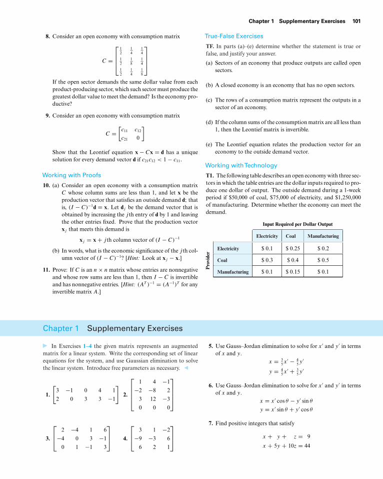
Chapter 1 Supplementary Exercises 101
8. Consider an open economy with consumption matrix
C =
⎡⎢⎢⎣
12
14
14
12
18
14
12
14
18
⎤⎥⎥⎦
If the open sector demands the same dollar value from eachproduct-producing sector, which such sector must produce thegreatest dollar value to meet the demand? Is the economy pro-ductive?
9. Consider an open economy with consumption matrix
C =[c11 c12
c21 0
]
Show that the Leontief equation x − Cx = d has a uniquesolution for every demand vector d if c21c12 < 1 − c11.
Working with Proofs
10. (a) Consider an open economy with a consumption matrixC whose column sums are less than 1, and let x be theproduction vector that satisfies an outside demand d; thatis, (I − C)−1d = x. Let dj be the demand vector that isobtained by increasing the j th entry of d by 1 and leavingthe other entries fixed. Prove that the production vectorxj that meets this demand is
xj = x + j th column vector of (I − C)−1
(b) In words, what is the economic significance of the j th col-umn vector of (I − C)−1? [Hint: Look at xj − x.]
11. Prove: If C is an n × n matrix whose entries are nonnegativeand whose row sums are less than 1, then I − C is invertibleand has nonnegative entries. [Hint: (AT )−1 = (A−1)T for anyinvertible matrix A.]
True-False Exercises
TF. In parts (a)–(e) determine whether the statement is true orfalse, and justify your answer.
(a) Sectors of an economy that produce outputs are called opensectors.
(b) A closed economy is an economy that has no open sectors.
(c) The rows of a consumption matrix represent the outputs in asector of an economy.
(d) If the column sums of the consumption matrix are all less than1, then the Leontief matrix is invertible.
(e) The Leontief equation relates the production vector for aneconomy to the outside demand vector.
Working withTechnology
T1. The following table describes an open economy with three sec-tors in which the table entries are the dollar inputs required to pro-duce one dollar of output. The outside demand during a 1-weekperiod if $50,000 of coal, $75,000 of electricity, and $1,250,000of manufacturing. Determine whether the economy can meet thedemand.
Pro
vide
r
Input Required per Dollar Output
Electricity Coal Manufacturing
Electricity $ 0.1 $ 0.25 $ 0.2
Coal $ 0.3 $ 0.4 $ 0.5
Manufacturing $ 0.1 $ 0.15 $ 0.1
Chapter 1 Supplementary Exercises
In Exercises 1–4 the given matrix represents an augmentedmatrix for a linear system. Write the corresponding set of linearequations for the system, and use Gaussian elimination to solvethe linear system. Introduce free parameters as necessary.
1.
[3 −1 0 4 1
2 0 3 3 −1
]2.
⎡⎢⎢⎢⎣
1 4 −1
−2 −8 2
3 12 −3
0 0 0
⎤⎥⎥⎥⎦
3.
⎡⎢⎣ 2 −4 1 6
−4 0 3 −1
0 1 −1 3
⎤⎥⎦ 4.
⎡⎢⎣ 3 1 −2
−9 −3 6
6 2 1
⎤⎥⎦
5. Use Gauss–Jordan elimination to solve for x ′ and y ′ in termsof x and y.
x = 35 x
′ − 45 y
′
y = 45 x
′ + 35 y
′
6. Use Gauss–Jordan elimination to solve for x ′ and y ′ in termsof x and y.
x = x ′ cos θ − y ′ sin θ
y = x ′ sin θ + y ′ cos θ
7. Find positive integers that satisfy
x + y + z = 9
x + 5y + 10z = 44
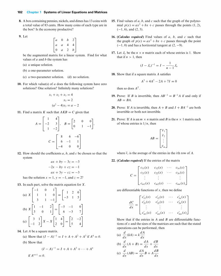
102 Chapter 1 Systems of Linear Equations and Matrices
8. A box containing pennies, nickels, and dimes has 13 coins witha total value of 83 cents. How many coins of each type are inthe box? Is the economy productive?
9. Let ⎡⎢⎣a 0 b 2
a a 4 4
0 a 2 b
⎤⎥⎦
be the augmented matrix for a linear system. Find for whatvalues of a and b the system has
(a) a unique solution.
(b) a one-parameter solution.
(c) a two-parameter solution. (d) no solution.
10. For which value(s) of a does the following system have zerosolutions? One solution? Infinitely many solutions?
x1 + x2 + x3 = 4
x3 = 2
(a2 − 4)x3 = a − 2
11. Find a matrix K such that AKB = C given that
A =⎡⎢⎣ 1 4
−2 3
1 −2
⎤⎥⎦, B =
[2 0 0
0 1 −1
],
C =⎡⎢⎣ 8 6 −6
6 −1 1
−4 0 0
⎤⎥⎦
12. How should the coefficients a, b, and c be chosen so that thesystem
ax + by − 3z = −3
−2x − by + cz = −1
ax + 3y − cz = −3
has the solution x = 1, y = −1, and z = 2?
13. In each part, solve the matrix equation for X.
(a) X
⎡⎢⎣−1 0 1
1 1 0
3 1 −1
⎤⎥⎦ =
[1 2 0
−3 1 5
]
(b) X
[1 −1 2
3 0 1
]=[−5 −1 0
6 −3 7
]
(c)
[3 1
−1 2
]X − X
[1 4
2 0
]=[
2 −2
5 4
]
14. Let A be a square matrix.
(a) Show that (I − A)−1 = I + A + A2 + A3 if A4 = 0.
(b) Show that
(I − A)−1 = I + A + A2 + · · · + An
if An+1 = 0.
15. Find values of a, b, and c such that the graph of the polyno-mial p(x) = ax2 + bx + c passes through the points (1, 2),(−1, 6), and (2, 3).
16. (Calculus required ) Find values of a, b, and c such thatthe graph of p(x) = ax2 + bx + c passes through the point(−1, 0) and has a horizontal tangent at (2,−9).
17. Let Jn be the n × n matrix each of whose entries is 1. Showthat if n > 1, then
(I − Jn)−1 = I − 1
n − 1Jn
18. Show that if a square matrix A satisfies
A3 + 4A2 − 2A + 7I = 0
then so does AT .
19. Prove: If B is invertible, then AB−1 = B−1A if and only ifAB = BA.
20. Prove: If A is invertible, then A + B and I + BA−1 are bothinvertible or both not invertible.
21. Prove: If A is an m × n matrix and B is the n × 1 matrix eachof whose entries is 1/n, then
AB =
⎡⎢⎢⎢⎣
r1
r2...
rm
⎤⎥⎥⎥⎦
where ri is the average of the entries in the ith row of A.
22. (Calculus required ) If the entries of the matrix
C =
⎡⎢⎢⎢⎣
c11(x) c12(x) · · · c1n(x)
c21(x) c22(x) · · · c2n(x)...
......
cm1(x) cm2(x) · · · cmn(x)
⎤⎥⎥⎥⎦
are differentiable functions of x, then we define
dC
dx=
⎡⎢⎢⎢⎣
c′11(x) c′
12(x) · · · c′1n(x)
c′21(x) c′
22(x) · · · c′2n(x)
......
...
c′m1(x) c′
m2(x) · · · c′mn(x)
⎤⎥⎥⎥⎦
Show that if the entries in A and B are differentiable func-tions of x and the sizes of the matrices are such that the statedoperations can be performed, then
(a)d
dx(kA) = k
dA
dx
(b)d
dx(A + B) = dA
dx+ dB
dx
(c)d
dx(AB) = dA
dxB + A
dB
dx
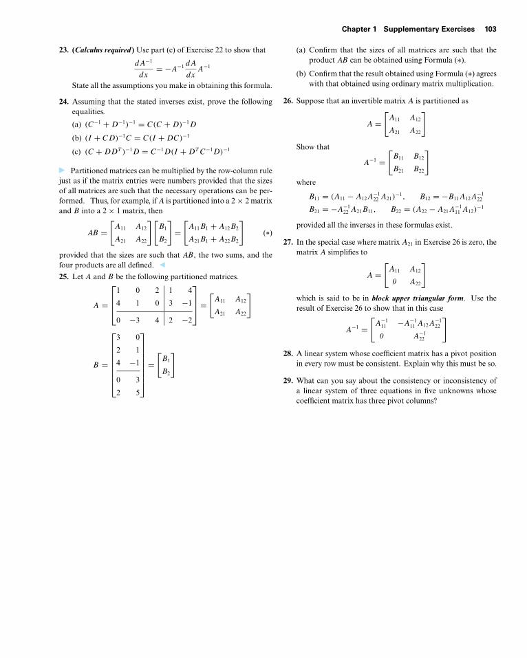
Chapter 1 Supplementary Exercises 103
23. (Calculus required ) Use part (c) of Exercise 22 to show that
dA−1
dx= −A−1 dA
dxA−1
State all the assumptions you make in obtaining this formula.
24. Assuming that the stated inverses exist, prove the followingequalities.
(a) (C−1 + D−1)−1 = C(C + D)−1D
(b) (I + CD)−1C = C(I + DC)−1
(c) (C + DDT )−1D = C−1D(I + DT C−1D)−1
Partitioned matrices can be multiplied by the row-column rulejust as if the matrix entries were numbers provided that the sizesof all matrices are such that the necessary operations can be per-formed. Thus, for example, if A is partitioned into a 2 × 2 matrixand B into a 2 × 1 matrix, then
AB =[A11 A12
A21 A22
][B1
B2
]=[A11B1 + A12B2
A21B1 + A22B2
](*)
provided that the sizes are such that AB, the two sums, and thefour products are all defined.
25. Let A and B be the following partitioned matrices.
A =
⎡⎢⎢⎣
1 0 2 1 4
4 1 0 3 −1
0 −3 4 2 −2
⎤⎥⎥⎦ =
[A11 A12
A21 A22
]
B =
⎡⎢⎢⎢⎢⎢⎢⎢⎣
3 0
2 1
4 −1
0 3
2 5
⎤⎥⎥⎥⎥⎥⎥⎥⎦
=[B1
B2
]
(a) Confirm that the sizes of all matrices are such that theproduct AB can be obtained using Formula (∗).
(b) Confirm that the result obtained using Formula (∗) agreeswith that obtained using ordinary matrix multiplication.
26. Suppose that an invertible matrix A is partitioned as
A =[A11 A12
A21 A22
]
Show that
A−1 =[B11 B12
B21 B22
]
where
B11 = (A11 − A12A−122 A21)
−1, B12 = −B11A12A−122
B21 = −A−122 A21B11, B22 = (A22 − A21A
−111 A12)
−1
provided all the inverses in these formulas exist.
27. In the special case where matrix A21 in Exercise 26 is zero, thematrix A simplifies to
A =[A11 A12
0 A22
]
which is said to be in block upper triangular form. Use theresult of Exercise 26 to show that in this case
A−1 =[A−1
11 −A−111 A12A
−122
0 A−122
]
28. A linear system whose coefficient matrix has a pivot positionin every row must be consistent. Explain why this must be so.
29. What can you say about the consistency or inconsistency ofa linear system of three equations in five unknowns whosecoefficient matrix has three pivot columns?